package ‘igraph’ - cran.microsoft.com · package ‘igraph ’ march 10, 2018 ... suggests ape,...
TRANSCRIPT
Package ‘igraph’March 10, 2018
Version 1.2.1
Title Network Analysis and Visualization
Author See AUTHORS file.
Maintainer Gábor Csárdi <[email protected]>
Description Routines for simple graphs and network analysis. It canhandle large graphs very well and provides functions for generating randomand regular graphs, graph visualization, centrality methods and much more.
Depends methods
Imports graphics, grDevices, magrittr, Matrix, pkgconfig (>= 2.0.0),stats, utils
Suggests ape, graph, igraphdata, rgl, scales, stats4, tcltk, testthat
License GPL (>= 2)
URL http://igraph.org
SystemRequirements gmp (optional), libxml2 (optional), glpk (optional)
BugReports https://github.com/igraph/igraph/issues
Encoding UTF-8
Collate 'adjacency.R' 'auto.R' 'assortativity.R' 'attributes.R''basic.R' 'bipartite.R' 'centrality.R' 'centralization.R''cliques.R' 'cocitation.R' 'cohesive.blocks.R' 'community.R''components.R' 'console.R' 'conversion.R' 'data_frame.R''decomposition.R' 'degseq.R' 'demo.R' 'embedding.R' 'epi.R''fit.R' 'flow.R' 'foreign.R' 'games.R' 'glet.R' 'hrg.R''igraph-package.R' 'incidence.R' 'indexing.R' 'interface.R''iterators.R' 'layout.R' 'layout_drl.R' 'lazyeval.R' 'make.R''minimum.spanning.tree.R' 'motifs.R' 'nexus.R' 'operators.R''other.R' 'package.R' 'palette.R' 'par.R' 'paths.R' 'plot.R''plot.common.R' 'plot.shapes.R' 'pp.R' 'print.R' 'printr.R''random_walk.R' 'rewire.R' 'scan.R' 'scg.R' 'sgm.R''similarity.R' 'simple.R' 'sir.R' 'socnet.R' 'sparsedf.R''structural.properties.R' 'structure.info.R' 'test.R''tkplot.R' 'topology.R' 'triangles.R' 'utils.R' 'uuid.R''versions.R' 'weakref.R' 'zzz-deprecate.R'
1

2 R topics documented:
NeedsCompilation yes
Repository CRAN
Date/Publication 2018-03-10 21:33:20 UTC
R topics documented:igraph-package . . . . . . . . . . . . . . . . . . . . . . . . . . . . . . . . . . . . . . . 9+.igraph . . . . . . . . . . . . . . . . . . . . . . . . . . . . . . . . . . . . . . . . . . . 11add_edges . . . . . . . . . . . . . . . . . . . . . . . . . . . . . . . . . . . . . . . . . . 14add_layout_ . . . . . . . . . . . . . . . . . . . . . . . . . . . . . . . . . . . . . . . . . 15add_vertices . . . . . . . . . . . . . . . . . . . . . . . . . . . . . . . . . . . . . . . . . 16adjacent_vertices . . . . . . . . . . . . . . . . . . . . . . . . . . . . . . . . . . . . . . 17all_simple_paths . . . . . . . . . . . . . . . . . . . . . . . . . . . . . . . . . . . . . . 17alpha_centrality . . . . . . . . . . . . . . . . . . . . . . . . . . . . . . . . . . . . . . . 18are_adjacent . . . . . . . . . . . . . . . . . . . . . . . . . . . . . . . . . . . . . . . . . 20arpack_defaults . . . . . . . . . . . . . . . . . . . . . . . . . . . . . . . . . . . . . . . 21articulation_points . . . . . . . . . . . . . . . . . . . . . . . . . . . . . . . . . . . . . 25as.directed . . . . . . . . . . . . . . . . . . . . . . . . . . . . . . . . . . . . . . . . . . 26as.igraph . . . . . . . . . . . . . . . . . . . . . . . . . . . . . . . . . . . . . . . . . . . 28assortativity . . . . . . . . . . . . . . . . . . . . . . . . . . . . . . . . . . . . . . . . . 29as_adjacency_matrix . . . . . . . . . . . . . . . . . . . . . . . . . . . . . . . . . . . . 31as_adj_list . . . . . . . . . . . . . . . . . . . . . . . . . . . . . . . . . . . . . . . . . . 32as_data_frame . . . . . . . . . . . . . . . . . . . . . . . . . . . . . . . . . . . . . . . . 33as_edgelist . . . . . . . . . . . . . . . . . . . . . . . . . . . . . . . . . . . . . . . . . . 35as_graphnel . . . . . . . . . . . . . . . . . . . . . . . . . . . . . . . . . . . . . . . . . 36as_ids . . . . . . . . . . . . . . . . . . . . . . . . . . . . . . . . . . . . . . . . . . . . 37as_incidence_matrix . . . . . . . . . . . . . . . . . . . . . . . . . . . . . . . . . . . . 38as_long_data_frame . . . . . . . . . . . . . . . . . . . . . . . . . . . . . . . . . . . . . 39as_membership . . . . . . . . . . . . . . . . . . . . . . . . . . . . . . . . . . . . . . . 40authority_score . . . . . . . . . . . . . . . . . . . . . . . . . . . . . . . . . . . . . . . 40automorphisms . . . . . . . . . . . . . . . . . . . . . . . . . . . . . . . . . . . . . . . 42bfs . . . . . . . . . . . . . . . . . . . . . . . . . . . . . . . . . . . . . . . . . . . . . . 43biconnected_components . . . . . . . . . . . . . . . . . . . . . . . . . . . . . . . . . . 45bipartite_mapping . . . . . . . . . . . . . . . . . . . . . . . . . . . . . . . . . . . . . . 47bipartite_projection . . . . . . . . . . . . . . . . . . . . . . . . . . . . . . . . . . . . . 48c.igraph.es . . . . . . . . . . . . . . . . . . . . . . . . . . . . . . . . . . . . . . . . . . 49c.igraph.vs . . . . . . . . . . . . . . . . . . . . . . . . . . . . . . . . . . . . . . . . . . 50canonical_permutation . . . . . . . . . . . . . . . . . . . . . . . . . . . . . . . . . . . 51categorical_pal . . . . . . . . . . . . . . . . . . . . . . . . . . . . . . . . . . . . . . . 53centralize . . . . . . . . . . . . . . . . . . . . . . . . . . . . . . . . . . . . . . . . . . 54centr_betw . . . . . . . . . . . . . . . . . . . . . . . . . . . . . . . . . . . . . . . . . . 55centr_betw_tmax . . . . . . . . . . . . . . . . . . . . . . . . . . . . . . . . . . . . . . 56centr_clo . . . . . . . . . . . . . . . . . . . . . . . . . . . . . . . . . . . . . . . . . . 57centr_clo_tmax . . . . . . . . . . . . . . . . . . . . . . . . . . . . . . . . . . . . . . . 58centr_degree . . . . . . . . . . . . . . . . . . . . . . . . . . . . . . . . . . . . . . . . . 59centr_degree_tmax . . . . . . . . . . . . . . . . . . . . . . . . . . . . . . . . . . . . . 60centr_eigen . . . . . . . . . . . . . . . . . . . . . . . . . . . . . . . . . . . . . . . . . 61

R topics documented: 3
centr_eigen_tmax . . . . . . . . . . . . . . . . . . . . . . . . . . . . . . . . . . . . . . 62cliques . . . . . . . . . . . . . . . . . . . . . . . . . . . . . . . . . . . . . . . . . . . . 63closeness . . . . . . . . . . . . . . . . . . . . . . . . . . . . . . . . . . . . . . . . . . 65cluster_edge_betweenness . . . . . . . . . . . . . . . . . . . . . . . . . . . . . . . . . 66cluster_fast_greedy . . . . . . . . . . . . . . . . . . . . . . . . . . . . . . . . . . . . . 68cluster_infomap . . . . . . . . . . . . . . . . . . . . . . . . . . . . . . . . . . . . . . . 70cluster_label_prop . . . . . . . . . . . . . . . . . . . . . . . . . . . . . . . . . . . . . . 71cluster_leading_eigen . . . . . . . . . . . . . . . . . . . . . . . . . . . . . . . . . . . . 73cluster_louvain . . . . . . . . . . . . . . . . . . . . . . . . . . . . . . . . . . . . . . . 75cluster_optimal . . . . . . . . . . . . . . . . . . . . . . . . . . . . . . . . . . . . . . . 76cluster_spinglass . . . . . . . . . . . . . . . . . . . . . . . . . . . . . . . . . . . . . . 78cluster_walktrap . . . . . . . . . . . . . . . . . . . . . . . . . . . . . . . . . . . . . . . 80cocitation . . . . . . . . . . . . . . . . . . . . . . . . . . . . . . . . . . . . . . . . . . 82cohesive_blocks . . . . . . . . . . . . . . . . . . . . . . . . . . . . . . . . . . . . . . . 83compare . . . . . . . . . . . . . . . . . . . . . . . . . . . . . . . . . . . . . . . . . . . 87complementer . . . . . . . . . . . . . . . . . . . . . . . . . . . . . . . . . . . . . . . . 88component_distribution . . . . . . . . . . . . . . . . . . . . . . . . . . . . . . . . . . . 89component_wise . . . . . . . . . . . . . . . . . . . . . . . . . . . . . . . . . . . . . . 91compose . . . . . . . . . . . . . . . . . . . . . . . . . . . . . . . . . . . . . . . . . . . 91consensus_tree . . . . . . . . . . . . . . . . . . . . . . . . . . . . . . . . . . . . . . . 93console . . . . . . . . . . . . . . . . . . . . . . . . . . . . . . . . . . . . . . . . . . . 94constraint . . . . . . . . . . . . . . . . . . . . . . . . . . . . . . . . . . . . . . . . . . 94contract . . . . . . . . . . . . . . . . . . . . . . . . . . . . . . . . . . . . . . . . . . . 96convex_hull . . . . . . . . . . . . . . . . . . . . . . . . . . . . . . . . . . . . . . . . . 97coreness . . . . . . . . . . . . . . . . . . . . . . . . . . . . . . . . . . . . . . . . . . . 98count_isomorphisms . . . . . . . . . . . . . . . . . . . . . . . . . . . . . . . . . . . . 99count_motifs . . . . . . . . . . . . . . . . . . . . . . . . . . . . . . . . . . . . . . . . 100count_subgraph_isomorphisms . . . . . . . . . . . . . . . . . . . . . . . . . . . . . . . 101count_triangles . . . . . . . . . . . . . . . . . . . . . . . . . . . . . . . . . . . . . . . 102curve_multiple . . . . . . . . . . . . . . . . . . . . . . . . . . . . . . . . . . . . . . . 103decompose . . . . . . . . . . . . . . . . . . . . . . . . . . . . . . . . . . . . . . . . . 104degree . . . . . . . . . . . . . . . . . . . . . . . . . . . . . . . . . . . . . . . . . . . . 105delete_edges . . . . . . . . . . . . . . . . . . . . . . . . . . . . . . . . . . . . . . . . . 106delete_edge_attr . . . . . . . . . . . . . . . . . . . . . . . . . . . . . . . . . . . . . . . 107delete_graph_attr . . . . . . . . . . . . . . . . . . . . . . . . . . . . . . . . . . . . . . 108delete_vertex_attr . . . . . . . . . . . . . . . . . . . . . . . . . . . . . . . . . . . . . . 109delete_vertices . . . . . . . . . . . . . . . . . . . . . . . . . . . . . . . . . . . . . . . 109dfs . . . . . . . . . . . . . . . . . . . . . . . . . . . . . . . . . . . . . . . . . . . . . . 110diameter . . . . . . . . . . . . . . . . . . . . . . . . . . . . . . . . . . . . . . . . . . . 112difference . . . . . . . . . . . . . . . . . . . . . . . . . . . . . . . . . . . . . . . . . . 114difference.igraph . . . . . . . . . . . . . . . . . . . . . . . . . . . . . . . . . . . . . . 114difference.igraph.es . . . . . . . . . . . . . . . . . . . . . . . . . . . . . . . . . . . . . 115difference.igraph.vs . . . . . . . . . . . . . . . . . . . . . . . . . . . . . . . . . . . . . 116dim_select . . . . . . . . . . . . . . . . . . . . . . . . . . . . . . . . . . . . . . . . . . 117disjoint_union . . . . . . . . . . . . . . . . . . . . . . . . . . . . . . . . . . . . . . . . 118distance_table . . . . . . . . . . . . . . . . . . . . . . . . . . . . . . . . . . . . . . . . 120diverging_pal . . . . . . . . . . . . . . . . . . . . . . . . . . . . . . . . . . . . . . . . 123diversity . . . . . . . . . . . . . . . . . . . . . . . . . . . . . . . . . . . . . . . . . . . 124

4 R topics documented:
dominator_tree . . . . . . . . . . . . . . . . . . . . . . . . . . . . . . . . . . . . . . . 125Drawing graphs . . . . . . . . . . . . . . . . . . . . . . . . . . . . . . . . . . . . . . . 127dyad_census . . . . . . . . . . . . . . . . . . . . . . . . . . . . . . . . . . . . . . . . . 133E . . . . . . . . . . . . . . . . . . . . . . . . . . . . . . . . . . . . . . . . . . . . . . . 134each_edge . . . . . . . . . . . . . . . . . . . . . . . . . . . . . . . . . . . . . . . . . . 135eccentricity . . . . . . . . . . . . . . . . . . . . . . . . . . . . . . . . . . . . . . . . . 136edge . . . . . . . . . . . . . . . . . . . . . . . . . . . . . . . . . . . . . . . . . . . . . 137edge_attr . . . . . . . . . . . . . . . . . . . . . . . . . . . . . . . . . . . . . . . . . . 138edge_attr<- . . . . . . . . . . . . . . . . . . . . . . . . . . . . . . . . . . . . . . . . . 139edge_attr_names . . . . . . . . . . . . . . . . . . . . . . . . . . . . . . . . . . . . . . 140edge_connectivity . . . . . . . . . . . . . . . . . . . . . . . . . . . . . . . . . . . . . . 141edge_density . . . . . . . . . . . . . . . . . . . . . . . . . . . . . . . . . . . . . . . . 142ego_size . . . . . . . . . . . . . . . . . . . . . . . . . . . . . . . . . . . . . . . . . . . 143eigen_centrality . . . . . . . . . . . . . . . . . . . . . . . . . . . . . . . . . . . . . . . 145embed_adjacency_matrix . . . . . . . . . . . . . . . . . . . . . . . . . . . . . . . . . . 147embed_laplacian_matrix . . . . . . . . . . . . . . . . . . . . . . . . . . . . . . . . . . 148ends . . . . . . . . . . . . . . . . . . . . . . . . . . . . . . . . . . . . . . . . . . . . . 150erdos.renyi.game . . . . . . . . . . . . . . . . . . . . . . . . . . . . . . . . . . . . . . 151estimate_betweenness . . . . . . . . . . . . . . . . . . . . . . . . . . . . . . . . . . . . 152fit_hrg . . . . . . . . . . . . . . . . . . . . . . . . . . . . . . . . . . . . . . . . . . . . 154fit_power_law . . . . . . . . . . . . . . . . . . . . . . . . . . . . . . . . . . . . . . . . 156get.edge.ids . . . . . . . . . . . . . . . . . . . . . . . . . . . . . . . . . . . . . . . . . 158girth . . . . . . . . . . . . . . . . . . . . . . . . . . . . . . . . . . . . . . . . . . . . . 159gorder . . . . . . . . . . . . . . . . . . . . . . . . . . . . . . . . . . . . . . . . . . . . 160graphlet_basis . . . . . . . . . . . . . . . . . . . . . . . . . . . . . . . . . . . . . . . . 161graph_ . . . . . . . . . . . . . . . . . . . . . . . . . . . . . . . . . . . . . . . . . . . . 163graph_attr . . . . . . . . . . . . . . . . . . . . . . . . . . . . . . . . . . . . . . . . . . 163graph_attr<- . . . . . . . . . . . . . . . . . . . . . . . . . . . . . . . . . . . . . . . . . 164graph_attr_names . . . . . . . . . . . . . . . . . . . . . . . . . . . . . . . . . . . . . . 165graph_from_adjacency_matrix . . . . . . . . . . . . . . . . . . . . . . . . . . . . . . . 166graph_from_adj_list . . . . . . . . . . . . . . . . . . . . . . . . . . . . . . . . . . . . . 168graph_from_atlas . . . . . . . . . . . . . . . . . . . . . . . . . . . . . . . . . . . . . . 170graph_from_edgelist . . . . . . . . . . . . . . . . . . . . . . . . . . . . . . . . . . . . 171graph_from_graphdb . . . . . . . . . . . . . . . . . . . . . . . . . . . . . . . . . . . . 172graph_from_graphnel . . . . . . . . . . . . . . . . . . . . . . . . . . . . . . . . . . . . 173graph_from_incidence_matrix . . . . . . . . . . . . . . . . . . . . . . . . . . . . . . . 175graph_from_isomorphism_class . . . . . . . . . . . . . . . . . . . . . . . . . . . . . . 176graph_from_lcf . . . . . . . . . . . . . . . . . . . . . . . . . . . . . . . . . . . . . . . 177graph_from_literal . . . . . . . . . . . . . . . . . . . . . . . . . . . . . . . . . . . . . 178graph_id . . . . . . . . . . . . . . . . . . . . . . . . . . . . . . . . . . . . . . . . . . . 180graph_version . . . . . . . . . . . . . . . . . . . . . . . . . . . . . . . . . . . . . . . . 181groups . . . . . . . . . . . . . . . . . . . . . . . . . . . . . . . . . . . . . . . . . . . . 181gsize . . . . . . . . . . . . . . . . . . . . . . . . . . . . . . . . . . . . . . . . . . . . . 182head_of . . . . . . . . . . . . . . . . . . . . . . . . . . . . . . . . . . . . . . . . . . . 183head_print . . . . . . . . . . . . . . . . . . . . . . . . . . . . . . . . . . . . . . . . . . 183hrg . . . . . . . . . . . . . . . . . . . . . . . . . . . . . . . . . . . . . . . . . . . . . . 184hrg-methods . . . . . . . . . . . . . . . . . . . . . . . . . . . . . . . . . . . . . . . . . 185hrg_tree . . . . . . . . . . . . . . . . . . . . . . . . . . . . . . . . . . . . . . . . . . . 185

R topics documented: 5
hub_score . . . . . . . . . . . . . . . . . . . . . . . . . . . . . . . . . . . . . . . . . . 186identical_graphs . . . . . . . . . . . . . . . . . . . . . . . . . . . . . . . . . . . . . . . 187igraph-attribute-combination . . . . . . . . . . . . . . . . . . . . . . . . . . . . . . . . 187igraph-dollar . . . . . . . . . . . . . . . . . . . . . . . . . . . . . . . . . . . . . . . . 189igraph-es-attributes . . . . . . . . . . . . . . . . . . . . . . . . . . . . . . . . . . . . . 190igraph-es-indexing . . . . . . . . . . . . . . . . . . . . . . . . . . . . . . . . . . . . . 192igraph-es-indexing2 . . . . . . . . . . . . . . . . . . . . . . . . . . . . . . . . . . . . . 194igraph-minus . . . . . . . . . . . . . . . . . . . . . . . . . . . . . . . . . . . . . . . . 195igraph-vs-attributes . . . . . . . . . . . . . . . . . . . . . . . . . . . . . . . . . . . . . 196igraph-vs-indexing . . . . . . . . . . . . . . . . . . . . . . . . . . . . . . . . . . . . . 197igraph-vs-indexing2 . . . . . . . . . . . . . . . . . . . . . . . . . . . . . . . . . . . . . 200igraph_demo . . . . . . . . . . . . . . . . . . . . . . . . . . . . . . . . . . . . . . . . 201igraph_options . . . . . . . . . . . . . . . . . . . . . . . . . . . . . . . . . . . . . . . 202igraph_test . . . . . . . . . . . . . . . . . . . . . . . . . . . . . . . . . . . . . . . . . . 204igraph_version . . . . . . . . . . . . . . . . . . . . . . . . . . . . . . . . . . . . . . . 204incident . . . . . . . . . . . . . . . . . . . . . . . . . . . . . . . . . . . . . . . . . . . 205incident_edges . . . . . . . . . . . . . . . . . . . . . . . . . . . . . . . . . . . . . . . 206indent_print . . . . . . . . . . . . . . . . . . . . . . . . . . . . . . . . . . . . . . . . . 206intersection . . . . . . . . . . . . . . . . . . . . . . . . . . . . . . . . . . . . . . . . . 207intersection.igraph . . . . . . . . . . . . . . . . . . . . . . . . . . . . . . . . . . . . . 207intersection.igraph.es . . . . . . . . . . . . . . . . . . . . . . . . . . . . . . . . . . . . 209intersection.igraph.vs . . . . . . . . . . . . . . . . . . . . . . . . . . . . . . . . . . . . 210isomorphic . . . . . . . . . . . . . . . . . . . . . . . . . . . . . . . . . . . . . . . . . 211isomorphisms . . . . . . . . . . . . . . . . . . . . . . . . . . . . . . . . . . . . . . . . 213isomorphism_class . . . . . . . . . . . . . . . . . . . . . . . . . . . . . . . . . . . . . 214is_bipartite . . . . . . . . . . . . . . . . . . . . . . . . . . . . . . . . . . . . . . . . . 214is_chordal . . . . . . . . . . . . . . . . . . . . . . . . . . . . . . . . . . . . . . . . . . 216is_dag . . . . . . . . . . . . . . . . . . . . . . . . . . . . . . . . . . . . . . . . . . . . 217is_degseq . . . . . . . . . . . . . . . . . . . . . . . . . . . . . . . . . . . . . . . . . . 218is_directed . . . . . . . . . . . . . . . . . . . . . . . . . . . . . . . . . . . . . . . . . . 219is_graphical . . . . . . . . . . . . . . . . . . . . . . . . . . . . . . . . . . . . . . . . . 220is_igraph . . . . . . . . . . . . . . . . . . . . . . . . . . . . . . . . . . . . . . . . . . 221is_matching . . . . . . . . . . . . . . . . . . . . . . . . . . . . . . . . . . . . . . . . . 221is_min_separator . . . . . . . . . . . . . . . . . . . . . . . . . . . . . . . . . . . . . . 223is_named . . . . . . . . . . . . . . . . . . . . . . . . . . . . . . . . . . . . . . . . . . 224is_printer_callback . . . . . . . . . . . . . . . . . . . . . . . . . . . . . . . . . . . . . 225is_separator . . . . . . . . . . . . . . . . . . . . . . . . . . . . . . . . . . . . . . . . . 226is_weighted . . . . . . . . . . . . . . . . . . . . . . . . . . . . . . . . . . . . . . . . . 226ivs . . . . . . . . . . . . . . . . . . . . . . . . . . . . . . . . . . . . . . . . . . . . . . 227keeping_degseq . . . . . . . . . . . . . . . . . . . . . . . . . . . . . . . . . . . . . . . 229knn . . . . . . . . . . . . . . . . . . . . . . . . . . . . . . . . . . . . . . . . . . . . . 230laplacian_matrix . . . . . . . . . . . . . . . . . . . . . . . . . . . . . . . . . . . . . . 231layout.fruchterman.reingold.grid . . . . . . . . . . . . . . . . . . . . . . . . . . . . . . 232layout.reingold.tilford . . . . . . . . . . . . . . . . . . . . . . . . . . . . . . . . . . . . 233layout.spring . . . . . . . . . . . . . . . . . . . . . . . . . . . . . . . . . . . . . . . . 233layout.svd . . . . . . . . . . . . . . . . . . . . . . . . . . . . . . . . . . . . . . . . . . 234layout_ . . . . . . . . . . . . . . . . . . . . . . . . . . . . . . . . . . . . . . . . . . . 234layout_as_bipartite . . . . . . . . . . . . . . . . . . . . . . . . . . . . . . . . . . . . . 235

6 R topics documented:
layout_as_star . . . . . . . . . . . . . . . . . . . . . . . . . . . . . . . . . . . . . . . . 237layout_as_tree . . . . . . . . . . . . . . . . . . . . . . . . . . . . . . . . . . . . . . . . 238layout_in_circle . . . . . . . . . . . . . . . . . . . . . . . . . . . . . . . . . . . . . . . 240layout_nicely . . . . . . . . . . . . . . . . . . . . . . . . . . . . . . . . . . . . . . . . 241layout_on_grid . . . . . . . . . . . . . . . . . . . . . . . . . . . . . . . . . . . . . . . 242layout_on_sphere . . . . . . . . . . . . . . . . . . . . . . . . . . . . . . . . . . . . . . 243layout_randomly . . . . . . . . . . . . . . . . . . . . . . . . . . . . . . . . . . . . . . 244layout_with_dh . . . . . . . . . . . . . . . . . . . . . . . . . . . . . . . . . . . . . . . 245layout_with_drl . . . . . . . . . . . . . . . . . . . . . . . . . . . . . . . . . . . . . . . 248layout_with_fr . . . . . . . . . . . . . . . . . . . . . . . . . . . . . . . . . . . . . . . . 250layout_with_gem . . . . . . . . . . . . . . . . . . . . . . . . . . . . . . . . . . . . . . 252layout_with_graphopt . . . . . . . . . . . . . . . . . . . . . . . . . . . . . . . . . . . . 253layout_with_kk . . . . . . . . . . . . . . . . . . . . . . . . . . . . . . . . . . . . . . . 255layout_with_lgl . . . . . . . . . . . . . . . . . . . . . . . . . . . . . . . . . . . . . . . 257layout_with_mds . . . . . . . . . . . . . . . . . . . . . . . . . . . . . . . . . . . . . . 258layout_with_sugiyama . . . . . . . . . . . . . . . . . . . . . . . . . . . . . . . . . . . 259local_scan . . . . . . . . . . . . . . . . . . . . . . . . . . . . . . . . . . . . . . . . . . 263make_ . . . . . . . . . . . . . . . . . . . . . . . . . . . . . . . . . . . . . . . . . . . . 265make_chordal_ring . . . . . . . . . . . . . . . . . . . . . . . . . . . . . . . . . . . . . 266make_clusters . . . . . . . . . . . . . . . . . . . . . . . . . . . . . . . . . . . . . . . . 267make_de_bruijn_graph . . . . . . . . . . . . . . . . . . . . . . . . . . . . . . . . . . . 267make_empty_graph . . . . . . . . . . . . . . . . . . . . . . . . . . . . . . . . . . . . . 268make_full_bipartite_graph . . . . . . . . . . . . . . . . . . . . . . . . . . . . . . . . . 269make_full_citation_graph . . . . . . . . . . . . . . . . . . . . . . . . . . . . . . . . . . 270make_full_graph . . . . . . . . . . . . . . . . . . . . . . . . . . . . . . . . . . . . . . 271make_graph . . . . . . . . . . . . . . . . . . . . . . . . . . . . . . . . . . . . . . . . . 272make_kautz_graph . . . . . . . . . . . . . . . . . . . . . . . . . . . . . . . . . . . . . 275make_lattice . . . . . . . . . . . . . . . . . . . . . . . . . . . . . . . . . . . . . . . . . 276make_line_graph . . . . . . . . . . . . . . . . . . . . . . . . . . . . . . . . . . . . . . 277make_ring . . . . . . . . . . . . . . . . . . . . . . . . . . . . . . . . . . . . . . . . . . 278make_star . . . . . . . . . . . . . . . . . . . . . . . . . . . . . . . . . . . . . . . . . . 279make_tree . . . . . . . . . . . . . . . . . . . . . . . . . . . . . . . . . . . . . . . . . . 280match_vertices . . . . . . . . . . . . . . . . . . . . . . . . . . . . . . . . . . . . . . . 281max_cardinality . . . . . . . . . . . . . . . . . . . . . . . . . . . . . . . . . . . . . . . 282max_flow . . . . . . . . . . . . . . . . . . . . . . . . . . . . . . . . . . . . . . . . . . 283membership . . . . . . . . . . . . . . . . . . . . . . . . . . . . . . . . . . . . . . . . . 285merge_coords . . . . . . . . . . . . . . . . . . . . . . . . . . . . . . . . . . . . . . . . 289min_cut . . . . . . . . . . . . . . . . . . . . . . . . . . . . . . . . . . . . . . . . . . . 290min_separators . . . . . . . . . . . . . . . . . . . . . . . . . . . . . . . . . . . . . . . 292min_st_separators . . . . . . . . . . . . . . . . . . . . . . . . . . . . . . . . . . . . . . 293modularity.igraph . . . . . . . . . . . . . . . . . . . . . . . . . . . . . . . . . . . . . . 294motifs . . . . . . . . . . . . . . . . . . . . . . . . . . . . . . . . . . . . . . . . . . . . 296mst . . . . . . . . . . . . . . . . . . . . . . . . . . . . . . . . . . . . . . . . . . . . . . 297neighbors . . . . . . . . . . . . . . . . . . . . . . . . . . . . . . . . . . . . . . . . . . 298normalize . . . . . . . . . . . . . . . . . . . . . . . . . . . . . . . . . . . . . . . . . . 299norm_coords . . . . . . . . . . . . . . . . . . . . . . . . . . . . . . . . . . . . . . . . 299page_rank . . . . . . . . . . . . . . . . . . . . . . . . . . . . . . . . . . . . . . . . . . 300path . . . . . . . . . . . . . . . . . . . . . . . . . . . . . . . . . . . . . . . . . . . . . 303

R topics documented: 7
permute . . . . . . . . . . . . . . . . . . . . . . . . . . . . . . . . . . . . . . . . . . . 304Pie charts as vertices . . . . . . . . . . . . . . . . . . . . . . . . . . . . . . . . . . . . 305plot.igraph . . . . . . . . . . . . . . . . . . . . . . . . . . . . . . . . . . . . . . . . . . 306plot.sir . . . . . . . . . . . . . . . . . . . . . . . . . . . . . . . . . . . . . . . . . . . . 307plot_dendrogram . . . . . . . . . . . . . . . . . . . . . . . . . . . . . . . . . . . . . . 309plot_dendrogram.igraphHRG . . . . . . . . . . . . . . . . . . . . . . . . . . . . . . . . 311power_centrality . . . . . . . . . . . . . . . . . . . . . . . . . . . . . . . . . . . . . . 313predict_edges . . . . . . . . . . . . . . . . . . . . . . . . . . . . . . . . . . . . . . . . 315print.igraph . . . . . . . . . . . . . . . . . . . . . . . . . . . . . . . . . . . . . . . . . 316print.igraph.es . . . . . . . . . . . . . . . . . . . . . . . . . . . . . . . . . . . . . . . . 318print.igraph.vs . . . . . . . . . . . . . . . . . . . . . . . . . . . . . . . . . . . . . . . . 319print.igraphHRG . . . . . . . . . . . . . . . . . . . . . . . . . . . . . . . . . . . . . . 321print.igraphHRGConsensus . . . . . . . . . . . . . . . . . . . . . . . . . . . . . . . . . 322print.nexusDatasetInfo . . . . . . . . . . . . . . . . . . . . . . . . . . . . . . . . . . . 323printer_callback . . . . . . . . . . . . . . . . . . . . . . . . . . . . . . . . . . . . . . . 326printr . . . . . . . . . . . . . . . . . . . . . . . . . . . . . . . . . . . . . . . . . . . . 327radius . . . . . . . . . . . . . . . . . . . . . . . . . . . . . . . . . . . . . . . . . . . . 327random_walk . . . . . . . . . . . . . . . . . . . . . . . . . . . . . . . . . . . . . . . . 328read_graph . . . . . . . . . . . . . . . . . . . . . . . . . . . . . . . . . . . . . . . . . 329reciprocity . . . . . . . . . . . . . . . . . . . . . . . . . . . . . . . . . . . . . . . . . . 330rep.igraph . . . . . . . . . . . . . . . . . . . . . . . . . . . . . . . . . . . . . . . . . . 331rev.igraph.es . . . . . . . . . . . . . . . . . . . . . . . . . . . . . . . . . . . . . . . . . 332rev.igraph.vs . . . . . . . . . . . . . . . . . . . . . . . . . . . . . . . . . . . . . . . . . 333rewire . . . . . . . . . . . . . . . . . . . . . . . . . . . . . . . . . . . . . . . . . . . . 333rglplot . . . . . . . . . . . . . . . . . . . . . . . . . . . . . . . . . . . . . . . . . . . . 334running_mean . . . . . . . . . . . . . . . . . . . . . . . . . . . . . . . . . . . . . . . . 335r_pal . . . . . . . . . . . . . . . . . . . . . . . . . . . . . . . . . . . . . . . . . . . . . 336sample_ . . . . . . . . . . . . . . . . . . . . . . . . . . . . . . . . . . . . . . . . . . . 336sample_bipartite . . . . . . . . . . . . . . . . . . . . . . . . . . . . . . . . . . . . . . . 337sample_correlated_gnp . . . . . . . . . . . . . . . . . . . . . . . . . . . . . . . . . . . 338sample_correlated_gnp_pair . . . . . . . . . . . . . . . . . . . . . . . . . . . . . . . . 339sample_degseq . . . . . . . . . . . . . . . . . . . . . . . . . . . . . . . . . . . . . . . 341sample_dirichlet . . . . . . . . . . . . . . . . . . . . . . . . . . . . . . . . . . . . . . . 342sample_dot_product . . . . . . . . . . . . . . . . . . . . . . . . . . . . . . . . . . . . . 343sample_fitness . . . . . . . . . . . . . . . . . . . . . . . . . . . . . . . . . . . . . . . . 344sample_fitness_pl . . . . . . . . . . . . . . . . . . . . . . . . . . . . . . . . . . . . . . 346sample_forestfire . . . . . . . . . . . . . . . . . . . . . . . . . . . . . . . . . . . . . . 347sample_gnm . . . . . . . . . . . . . . . . . . . . . . . . . . . . . . . . . . . . . . . . . 349sample_gnp . . . . . . . . . . . . . . . . . . . . . . . . . . . . . . . . . . . . . . . . . 350sample_grg . . . . . . . . . . . . . . . . . . . . . . . . . . . . . . . . . . . . . . . . . 351sample_growing . . . . . . . . . . . . . . . . . . . . . . . . . . . . . . . . . . . . . . . 352sample_hierarchical_sbm . . . . . . . . . . . . . . . . . . . . . . . . . . . . . . . . . . 353sample_hrg . . . . . . . . . . . . . . . . . . . . . . . . . . . . . . . . . . . . . . . . . 354sample_islands . . . . . . . . . . . . . . . . . . . . . . . . . . . . . . . . . . . . . . . 355sample_k_regular . . . . . . . . . . . . . . . . . . . . . . . . . . . . . . . . . . . . . . 356sample_last_cit . . . . . . . . . . . . . . . . . . . . . . . . . . . . . . . . . . . . . . . 357sample_motifs . . . . . . . . . . . . . . . . . . . . . . . . . . . . . . . . . . . . . . . . 358sample_pa . . . . . . . . . . . . . . . . . . . . . . . . . . . . . . . . . . . . . . . . . . 359

8 R topics documented:
sample_pa_age . . . . . . . . . . . . . . . . . . . . . . . . . . . . . . . . . . . . . . . 361sample_pref . . . . . . . . . . . . . . . . . . . . . . . . . . . . . . . . . . . . . . . . . 363sample_sbm . . . . . . . . . . . . . . . . . . . . . . . . . . . . . . . . . . . . . . . . . 365sample_seq . . . . . . . . . . . . . . . . . . . . . . . . . . . . . . . . . . . . . . . . . 366sample_smallworld . . . . . . . . . . . . . . . . . . . . . . . . . . . . . . . . . . . . . 367sample_sphere_surface . . . . . . . . . . . . . . . . . . . . . . . . . . . . . . . . . . . 368sample_sphere_volume . . . . . . . . . . . . . . . . . . . . . . . . . . . . . . . . . . . 369sample_traits_callaway . . . . . . . . . . . . . . . . . . . . . . . . . . . . . . . . . . . 370scan_stat . . . . . . . . . . . . . . . . . . . . . . . . . . . . . . . . . . . . . . . . . . . 371scg . . . . . . . . . . . . . . . . . . . . . . . . . . . . . . . . . . . . . . . . . . . . . . 372scg-method . . . . . . . . . . . . . . . . . . . . . . . . . . . . . . . . . . . . . . . . . 376scg_eps . . . . . . . . . . . . . . . . . . . . . . . . . . . . . . . . . . . . . . . . . . . 377scg_group . . . . . . . . . . . . . . . . . . . . . . . . . . . . . . . . . . . . . . . . . . 378scg_semi_proj . . . . . . . . . . . . . . . . . . . . . . . . . . . . . . . . . . . . . . . . 380sequential_pal . . . . . . . . . . . . . . . . . . . . . . . . . . . . . . . . . . . . . . . . 382set_edge_attr . . . . . . . . . . . . . . . . . . . . . . . . . . . . . . . . . . . . . . . . 383set_graph_attr . . . . . . . . . . . . . . . . . . . . . . . . . . . . . . . . . . . . . . . . 384set_vertex_attr . . . . . . . . . . . . . . . . . . . . . . . . . . . . . . . . . . . . . . . . 385shapes . . . . . . . . . . . . . . . . . . . . . . . . . . . . . . . . . . . . . . . . . . . . 386similarity . . . . . . . . . . . . . . . . . . . . . . . . . . . . . . . . . . . . . . . . . . 390simplified . . . . . . . . . . . . . . . . . . . . . . . . . . . . . . . . . . . . . . . . . . 391simplify . . . . . . . . . . . . . . . . . . . . . . . . . . . . . . . . . . . . . . . . . . . 392spectrum . . . . . . . . . . . . . . . . . . . . . . . . . . . . . . . . . . . . . . . . . . . 393split_join_distance . . . . . . . . . . . . . . . . . . . . . . . . . . . . . . . . . . . . . 395srand . . . . . . . . . . . . . . . . . . . . . . . . . . . . . . . . . . . . . . . . . . . . . 396stochastic_matrix . . . . . . . . . . . . . . . . . . . . . . . . . . . . . . . . . . . . . . 396strength . . . . . . . . . . . . . . . . . . . . . . . . . . . . . . . . . . . . . . . . . . . 397st_cuts . . . . . . . . . . . . . . . . . . . . . . . . . . . . . . . . . . . . . . . . . . . . 398st_min_cuts . . . . . . . . . . . . . . . . . . . . . . . . . . . . . . . . . . . . . . . . . 399subcomponent . . . . . . . . . . . . . . . . . . . . . . . . . . . . . . . . . . . . . . . . 401subgraph . . . . . . . . . . . . . . . . . . . . . . . . . . . . . . . . . . . . . . . . . . . 402subgraph_centrality . . . . . . . . . . . . . . . . . . . . . . . . . . . . . . . . . . . . . 403subgraph_isomorphic . . . . . . . . . . . . . . . . . . . . . . . . . . . . . . . . . . . . 404subgraph_isomorphisms . . . . . . . . . . . . . . . . . . . . . . . . . . . . . . . . . . 406tail_of . . . . . . . . . . . . . . . . . . . . . . . . . . . . . . . . . . . . . . . . . . . . 407time_bins.sir . . . . . . . . . . . . . . . . . . . . . . . . . . . . . . . . . . . . . . . . . 408tkigraph . . . . . . . . . . . . . . . . . . . . . . . . . . . . . . . . . . . . . . . . . . . 410tkplot . . . . . . . . . . . . . . . . . . . . . . . . . . . . . . . . . . . . . . . . . . . . 410topo_sort . . . . . . . . . . . . . . . . . . . . . . . . . . . . . . . . . . . . . . . . . . 413transitivity . . . . . . . . . . . . . . . . . . . . . . . . . . . . . . . . . . . . . . . . . . 414triad_census . . . . . . . . . . . . . . . . . . . . . . . . . . . . . . . . . . . . . . . . . 416unfold_tree . . . . . . . . . . . . . . . . . . . . . . . . . . . . . . . . . . . . . . . . . 418union . . . . . . . . . . . . . . . . . . . . . . . . . . . . . . . . . . . . . . . . . . . . 419union.igraph . . . . . . . . . . . . . . . . . . . . . . . . . . . . . . . . . . . . . . . . . 419union.igraph.es . . . . . . . . . . . . . . . . . . . . . . . . . . . . . . . . . . . . . . . 420union.igraph.vs . . . . . . . . . . . . . . . . . . . . . . . . . . . . . . . . . . . . . . . 421unique.igraph.es . . . . . . . . . . . . . . . . . . . . . . . . . . . . . . . . . . . . . . . 422unique.igraph.vs . . . . . . . . . . . . . . . . . . . . . . . . . . . . . . . . . . . . . . . 423

igraph-package 9
upgrade_graph . . . . . . . . . . . . . . . . . . . . . . . . . . . . . . . . . . . . . . . 424V . . . . . . . . . . . . . . . . . . . . . . . . . . . . . . . . . . . . . . . . . . . . . . 424vertex . . . . . . . . . . . . . . . . . . . . . . . . . . . . . . . . . . . . . . . . . . . . 426vertex_attr . . . . . . . . . . . . . . . . . . . . . . . . . . . . . . . . . . . . . . . . . . 427vertex_attr<- . . . . . . . . . . . . . . . . . . . . . . . . . . . . . . . . . . . . . . . . . 428vertex_attr_names . . . . . . . . . . . . . . . . . . . . . . . . . . . . . . . . . . . . . . 429vertex_connectivity . . . . . . . . . . . . . . . . . . . . . . . . . . . . . . . . . . . . . 429which_multiple . . . . . . . . . . . . . . . . . . . . . . . . . . . . . . . . . . . . . . . 431which_mutual . . . . . . . . . . . . . . . . . . . . . . . . . . . . . . . . . . . . . . . . 433without_attr . . . . . . . . . . . . . . . . . . . . . . . . . . . . . . . . . . . . . . . . . 434without_loops . . . . . . . . . . . . . . . . . . . . . . . . . . . . . . . . . . . . . . . . 434without_multiples . . . . . . . . . . . . . . . . . . . . . . . . . . . . . . . . . . . . . . 435with_edge_ . . . . . . . . . . . . . . . . . . . . . . . . . . . . . . . . . . . . . . . . . 435with_graph_ . . . . . . . . . . . . . . . . . . . . . . . . . . . . . . . . . . . . . . . . . 436with_igraph_opt . . . . . . . . . . . . . . . . . . . . . . . . . . . . . . . . . . . . . . . 436with_vertex_ . . . . . . . . . . . . . . . . . . . . . . . . . . . . . . . . . . . . . . . . 437write_graph . . . . . . . . . . . . . . . . . . . . . . . . . . . . . . . . . . . . . . . . . 437[.igraph . . . . . . . . . . . . . . . . . . . . . . . . . . . . . . . . . . . . . . . . . . . 439[[.igraph . . . . . . . . . . . . . . . . . . . . . . . . . . . . . . . . . . . . . . . . . . . 441%>% . . . . . . . . . . . . . . . . . . . . . . . . . . . . . . . . . . . . . . . . . . . . 443
Index 444
igraph-package The igraph package
Description
igraph is a library and R package for network analysis.
Introduction
The main goals of the igraph library is to provide a set of data types and functions for 1) pain-freeimplementation of graph algorithms, 2) fast handling of large graphs, with millions of vertices andedges, 3) allowing rapid prototyping via high level languages like R.
Igraph graphs
Igraph graphs have a class ‘igraph’. They are printed to the screen in a special format, here is anexample, a ring graph created using make_ring:
IGRAPH U--- 10 10 -- Ring graph+ attr: name (g/c), mutual (g/x), circular (g/x)
‘IGRAPH’ denotes that this is an igraph graph. Then come four bits that denote the kind of thegraph: the first is ‘U’ for undirected and ‘D’ for directed graphs. The second is ‘N’ for named graph(i.e. if the graph has the ‘name’ vertex attribute set). The third is ‘W’ for weighted graphs (i.e. if
10 igraph-package
the ‘weight’ edge attribute is set). The fourth is ‘B’ for bipartite graphs (i.e. if the ‘type’ vertexattribute is set).
Then come two numbers, the number of vertices and the number of edges in the graph, and after adouble dash, the name of the graph (the ‘name’ graph attribute) is printed if present. The second lineis optional and it contains all the attributes of the graph. This graph has a ‘name’ graph attribute,of type character, and two other graph attributes called ‘mutual’ and ‘circular’, of a complextype. A complex type is simply anything that is not numeric or character. See the documentation ofprint.igraph for details.
If you want to see the edges of the graph as well, then use the print_all function:
> print_all(g)IGRAPH badcafe U--- 10 10 -- Ring graph+ attr: name (g/c), mutual (g/x), circular (g/x)+ edges:[1] 1-- 2 2-- 3 3-- 4 4-- 5 5-- 6 6-- 7 7-- 8 8-- 9 9--10 1--10
Creating graphs
There are many functions in igraph for creating graphs, both deterministic and stochastic; stochasticgraph constructors are called ‘games’.
To create small graphs with a given structure probably the graph_from_literal function is eas-iest. It uses R’s formula interface, its manual page contains many examples. Another option isgraph, which takes numeric vertex ids directly. graph.atlas creates graph from the Graph Atlas,make_graph can create some special graphs.
To create graphs from field data, graph_from_edgelist, graph_from_data_frame and graph_from_adjacency_matrixare probably the best choices.
The igraph package includes some classic random graphs like the Erdos-Renyi GNP and GNMgraphs (sample_gnp, sample_gnm) and some recent popular models, like preferential attachment(sample_pa) and the small-world model (sample_smallworld).
Vertex and edge IDs
Vertices and edges have numerical vertex ids in igraph. Vertex ids are always consecutive and theystart with one. I.e. for a graph with n vertices the vertex ids are between 1 and n. If some operationchanges the number of vertices in the graphs, e.g. a subgraph is created via induced_subgraph,then the vertices are renumbered to satisfty this criteria.
The same is true for the edges as well, edge ids are always between one and m, the total number ofedges in the graph.
It is often desirable to follow vertices along a number of graph operations, and vertex ids don’tallow this because of the renumbering. The solution is to assign attributes to the vertices. These arekept by all operations, if possible. See more about attributes in the next section.
Attributes
In igraph it is possible to assign attributes to the vertices or edges of a graph, or to the graph itself.igraph provides flexible constructs for selecting a set of vertices or edges based on their attributevalues, see vertex_attr, V and E for details.
+.igraph 11
Some vertex/edge/graph attributes are treated specially. One of them is the ‘name’ attribute. This isused for printing the graph instead of the numerical ids, if it exists. Vertex names can also be usedto specify a vector or set of vertices, in all igraph functions. E.g. degree has a v argument that givesthe vertices for which the degree is calculated. This argument can be given as a character vector ofvertex names.
Edges can also have a ‘name’ attribute, and this is treated specially as well. Just like for vertices,edges can also be selected based on their names, e.g. in the delete_edges and other functions.
We note here, that vertex names can also be used to select edges. The form ‘from|to’, where ‘from’and ‘to’ are vertex names, select a single, possibly directed, edge going from ‘from’ to ‘to’. Thetwo forms can also be mixed in the same edge selector.
Other attributes define visualization parameters, see igraph.plotting for details.
Attribute values can be set to any R object, but note that storing the graph in some file formats mightresult the loss of complex attribute values. All attribute values are preserved if you use save andload to store/retrieve your graphs.
Visualization
igraph provides three different ways for visualization. The first is the plot.igraph function. (Ac-tually you don’t need to write plot.igraph, plot is enough. This function uses regular R graphicsand can be used with any R device.
The second function is tkplot, which uses a Tk GUI for basic interactive graph manipulation. (Tkis quite resource hungry, so don’t try this for very large graphs.)
The third way requires the rgl package and uses OpenGL. See the rglplot function for the details.
Make sure you read igraph.plotting before you start plotting your graphs.
File formats
igraph can handle various graph file formats, usually both for reading and writing. We suggest thatyou use the GraphML file format for your graphs, except if the graphs are too big. For big graphs asimpler format is recommended. See read_graph and write_graph for details.
Further information
The igraph homepage is at http://igraph.org. See especially the documentation section. Jointhe igraph-help mailing list if you have questions or comments.
+.igraph Add vertices, edges or another graph to a graph
Description
Add vertices, edges or another graph to a graph
12 +.igraph
Usage
## S3 method for class 'igraph'e1 + e2
Arguments
e1 First argument, probably an igraph graph, but see details below.
e2 Second argument, see details below.
Details
The plus operator can be used to add vertices or edges to graph. The actual operation that is per-formed depends on the type of the right hand side argument.
• If is is another igraph graph object and they are both named graphs, then the union of the twographs are calculated, see union.
• If it is another igraph graph object, but either of the two are not named, then the disjoint unionof the two graphs is calculated, see disjoint_union.
• If it is a numeric scalar, then the specified number of vertices are added to the graph.
• If it is a character scalar or vector, then it is interpreted as the names of the vertices to add tothe graph.
• If it is an object created with the vertex or vertices function, then new vertices are added tothe graph. This form is appropriate when one wants to add some vertex attributes as well. Theoperands of the vertices function specifies the number of vertices to add and their attributesas well.The unnamed arguments of vertices are concatenated and used as the ‘name’ vertex attribute(i.e. vertex names), the named arguments will be added as additional vertex attributes. Exam-ples:
g <- g +vertex(shape="circle", color= "red")
g <- g + vertex("foo", color="blue")g <- g + vertex("bar", "foobar")g <- g + vertices("bar2", "foobar2", color=1:2, shape="rectangle")
vertex is just an alias to vertices, and it is provided for readability. The user should use itif a single vertex is added to the graph.
• If it is an object created with the edge or edges function, then new edges will be added to thegraph. The new edges and possibly their attributes can be specified as the arguments of theedges function.The unnamed arguments of edges are concatenated and used as vertex ids of the end pointsof the new edges. The named arguments will be added as edge attributes.Examples:
g <- make_empty_graph() +vertices(letters[1:10]) +vertices("foo", "bar", "bar2", "foobar2")
g <- g + edge("a", "b")

+.igraph 13
g <- g + edges("foo", "bar", "bar2", "foobar2")g <- g + edges(c("bar", "foo", "foobar2", "bar2"), color="red", weight=1:2)
See more examples below.edge is just an alias to edges and it is provided for readability. The user should use it if asingle edge is added to the graph.
• If it is an object created with the path function, then new edges that form a path are added.The edges and possibly their attributes are specified as the arguments to the path function.The non-named arguments are concatenated and interpreted as the vertex ids along the path.The remaining arguments are added as edge attributes.Examples:
g <- make_empty_graph() + vertices(letters[1:10])g <- g + path("a", "b", "c", "d")g <- g + path("e", "f", "g", weight=1:2, color="red")g <- g + path(c("f", "c", "j", "d"), width=1:3, color="green")
It is important to note that, although the plus operator is commutative, i.e. is possible to write
graph <- "foo" + make_empty_graph()
it is not associative, e.g.
graph <- "foo" + "bar" + make_empty_graph()
results a syntax error, unless parentheses are used:
graph <- "foo" + ( "bar" + make_empty_graph() )
For clarity, we suggest to always put the graph object on the left hand side of the operator:
graph <- make_empty_graph() + "foo" + "bar"
See Also
Other functions for manipulating graph structure: add_edges, add_vertices, delete_edges,delete_vertices, edge, igraph-minus, path, vertex
Examples
# 10 vertices named a,b,c,... and no edgesg <- make_empty_graph() + vertices(letters[1:10])
# Add edges to make it a ringg <- g + path(letters[1:10], letters[1], color = "grey")
# Add some extra random edgesg <- g + edges(sample(V(g), 10, replace = TRUE), color = "red")g$layout <- layout_in_circleplot(g)
14 add_edges
add_edges Add edges to a graph
Description
The new edges are given as a vertex sequence, e.g. internal numeric vertex ids, or vertex names.The first edge points from edges[1] to edges[2], the second from edges[3] to edges[4], etc.
Usage
add_edges(graph, edges, ..., attr = list())
Arguments
graph The input graph
edges The edges to add, a vertex sequence with even number of vertices.
... Additional arguments, they must be named, and they will be added as edgeattributes, for the newly added edges. See also details below.
attr A named list, its elements will be added as edge attributes, for the newly addededges. See also details below.
Details
If attributes are supplied, and they are not present in the graph, their values for the original edges ofthe graph are set to NA.
Value
The graph, with the edges (and attributes) added.
See Also
Other functions for manipulating graph structure: +.igraph, add_vertices, delete_edges, delete_vertices,edge, igraph-minus, path, vertex
Examples
g <- make_empty_graph(n = 5) %>%add_edges(c(1,2, 2,3, 3,4, 4,5)) %>%set_edge_attr("color", value = "red") %>%add_edges(c(5,1), color = "green")
E(g)[[]]plot(g)

add_layout_ 15
add_layout_ Add layout to graph
Description
Add layout to graph
Usage
add_layout_(graph, ..., overwrite = TRUE)
Arguments
graph The input graph.
... Additional arguments are passed to layout_.
overwrite Whether to overwrite the layout of the graph, if it already has one.
Value
The input graph, with the layout added.
See Also
layout_ for a description of the layout API.
Other graph layouts: component_wise, layout_as_bipartite, layout_as_star, layout_as_tree,layout_in_circle, layout_nicely, layout_on_grid, layout_on_sphere, layout_randomly,layout_with_dh, layout_with_fr, layout_with_gem, layout_with_graphopt, layout_with_kk,layout_with_lgl, layout_with_mds, layout_with_sugiyama, layout_, merge_coords, norm_coords,normalize
Examples
(make_star(11) + make_star(11)) %>%add_layout_(as_star(), component_wise()) %>%plot()
16 add_vertices
add_vertices Add vertices to a graph
Description
If attributes are supplied, and they are not present in the graph, their values for the original verticesof the graph are set to NA.
Usage
add_vertices(graph, nv, ..., attr = list())
Arguments
graph The input graph.
nv The number of vertices to add.
... Additional arguments, they must be named, and they will be added as vertexattributes, for the newly added vertices. See also details below.
attr A named list, its elements will be added as vertex attributes, for the newly addedvertices. See also details below.
Value
The graph, with the vertices (and attributes) added.
See Also
Other functions for manipulating graph structure: +.igraph, add_edges, delete_edges, delete_vertices,edge, igraph-minus, path, vertex
Examples
g <- make_empty_graph() %>%add_vertices(3, color = "red") %>%add_vertices(2, color = "green") %>%add_edges(c(1,2, 2,3, 3,4, 4,5))
gV(g)[[]]plot(g)

adjacent_vertices 17
adjacent_vertices Adjacent vertices of multiple vertices in a graph
Description
This function is similar to neighbors, but it queries the adjacent vertices for multiple vertices atonce.
Usage
adjacent_vertices(graph, v, mode = c("out", "in", "all", "total"))
Arguments
graph Input graph.
v The vertices to query.
mode Whether to query outgoing (‘out’), incoming (‘in’) edges, or both types (‘all’).This is ignored for undirected graphs.
Value
A list of vertex sequences.
See Also
Other structural queries: [.igraph, [[.igraph, are_adjacent, ends, get.edge.ids, gorder,gsize, head_of, incident_edges, incident, is_directed, neighbors, tail_of
Examples
g <- make_graph("Zachary")adjacent_vertices(g, c(1, 34))
all_simple_paths List all simple paths from one source
Description
This function lists are simple paths from one source vertex to another vertex or vertices. A path issimple if the vertices it visits are not visited more than once.
Usage
all_simple_paths(graph, from, to = V(graph), mode = c("out", "in", "all","total"))

18 alpha_centrality
Arguments
graph The input graph.
from The source vertex.
to The target vertex of vertices. Defaults to all vertices.
mode Character constant, gives whether the shortest paths to or from the given ver-tices should be calculated for directed graphs. If out then the shortest pathsfrom the vertex, if in then to it will be considered. If all, the default, then thecorresponding undirected graph will be used, ie. not directed paths are searched.This argument is ignored for undirected graphs.
Details
Note that potentially there are exponentially many paths between two vertices of a graph, and youmay run out of memory when using this function, if your graph is lattice-like.
This function currently ignored multiple and loop edges.
Value
A list of integer vectors, each integer vector is a path from the source vertex to one of the targetvertices. A path is given by its vertex ids.
Examples
g <- make_ring(10)all_simple_paths(g, 1, 5)all_simple_paths(g, 1, c(3,5))
alpha_centrality Find Bonacich alpha centrality scores of network positions
Description
alpha_centrality calculates the alpha centrality of some (or all) vertices in a graph.
Usage
alpha_centrality(graph, nodes = V(graph), alpha = 1, loops = FALSE,exo = 1, weights = NULL, tol = 1e-07, sparse = TRUE)

alpha_centrality 19
Arguments
graph The input graph, can be directed or undirected
nodes Vertex sequence, the vertices for which the alpha centrality values are returned.(For technical reasons they will be calculated for all vertices, anyway.)
alpha Parameter specifying the relative importance of endogenous versus exogenousfactors in the determination of centrality. See details below.
loops Whether to eliminate loop edges from the graph before the calculation.
exo The exogenous factors, in most cases this is either a constant – the same factorfor every node, or a vector giving the factor for every vertex. Note that too longvectors will be truncated and too short vectors will be replicated to match thenumber of vertices.
weights A character scalar that gives the name of the edge attribute to use in the adja-cency matrix. If it is NULL, then the ‘weight’ edge attribute of the graph is used,if there is one. Otherwise, or if it is NA, then the calculation uses the standardadjacency matrix.
tol Tolerance for near-singularities during matrix inversion, see solve.
sparse Logical scalar, whether to use sparse matrices for the calculation. The ‘Matrix’package is required for sparse matrix support
Details
The alpha centrality measure can be considered as a generalization of eigenvector centerality todirected graphs. It was proposed by Bonacich in 2001 (see reference below).
The alpha centrality of the vertices in a graph is defined as the solution of the following matrixequation:
x = αATx+ e,
where A is the (not neccessarily symmetric) adjacency matrix of the graph, e is the vector of ex-ogenous sources of status of the vertices and α is the relative importance of the endogenous versusexogenous factors.
Value
A numeric vector contaning the centrality scores for the selected vertices.
Warning
Singular adjacency matrices cause problems for this algorithm, the routine may fail is certain cases.
Author(s)
Gabor Csardi <[email protected]>
References
Bonacich, P. and Lloyd, P. (2001). “Eigenvector-like measures of centrality for asymmetric rela-tions” Social Networks, 23, 191-201.
20 are_adjacent
See Also
eigen_centrality and power_centrality
Examples
# The examples from Bonacich's paperg.1 <- graph( c(1,3,2,3,3,4,4,5) )g.2 <- graph( c(2,1,3,1,4,1,5,1) )g.3 <- graph( c(1,2,2,3,3,4,4,1,5,1) )alpha_centrality(g.1)alpha_centrality(g.2)alpha_centrality(g.3,alpha=0.5)
are_adjacent Are two vertices adjacent?
Description
The order of the vertices only matters in directed graphs, where the existence of a directed (v1, v2)edge is queried.
Usage
are_adjacent(graph, v1, v2)
Arguments
graph The graph.
v1 The first vertex, tail in directed graphs.
v2 The second vertex, head in directed graphs.
Value
A logical scalar, TRUE is a (v1, v2) exists in the graph.
See Also
Other structural queries: [.igraph, [[.igraph, adjacent_vertices, ends, get.edge.ids, gorder,gsize, head_of, incident_edges, incident, is_directed, neighbors, tail_of

arpack_defaults 21
Examples
ug <- make_ring(10)ugare_adjacent(ug, 1, 2)are_adjacent(ug, 2, 1)
dg <- make_ring(10, directed = TRUE)dgare_adjacent(ug, 1, 2)are_adjacent(ug, 2, 1)
arpack_defaults ARPACK eigenvector calculation
Description
Interface to the ARPACK library for calculating eigenvectors of sparse matrices
Usage
arpack_defaults
arpack(func, extra = NULL, sym = FALSE, options = arpack_defaults,env = parent.frame(), complex = !sym)
Arguments
func The function to perform the matrix-vector multiplication. ARPACK requires toperform these by the user. The function gets the vector x as the first argument,and it should return Ax, where A is the “input matrix”. (The input matrix isnever given explicitly.) The second argument is extra.
extra Extra argument to supply to func.
sym Logical scalar, whether the input matrix is symmetric. Always supply TRUE hereif it is, since it can speed up the computation.
options Options to ARPACK, a named list to overwrite some of the default option values.See details below.
env The environment in which func will be evaluated.
complex Whether to convert the eigenvectors returned by ARPACK into R complex vec-tors. By default this is not done for symmetric problems (these only havereal eigenvectors/values), but only non-symmetric ones. If you have a non-symmetric problem, but you’re sure that the results will be real, then supplyFALSE here.
Format
An object of class list of length 14.

22 arpack_defaults
Details
ARPACK is a library for solving large scale eigenvalue problems. The package is designed tocompute a few eigenvalues and corresponding eigenvectors of a general n by n matrix A. It is mostappropriate for large sparse or structured matrices A where structured means that a matrix-vectorproduct w <- Av requires order n rather than the usual order n2 floating point operations. Pleasesee http://www.caam.rice.edu/software/ARPACK/ for details.
This function is an interface to ARPACK. igraph does not contain all ARPACK routines, only theones dealing with symmetric and non-symmetric eigenvalue problems using double precision realnumbers.
The eigenvalue calculation in ARPACK (in the simplest case) involves the calculation of the Avproduct where A is the matrix we work with and v is an arbitrary vector. The function supplied inthe fun argument is expected to perform this product. If the product can be done efficiently, e.g. ifthe matrix is sparse, then arpack is usually able to calculate the eigenvalues very quickly.
The options argument specifies what kind of calculation to perform. It is a list with the followingmembers, they correspond directly to ARPACK parameters. On input it has the following fields:
bmat Character constant, possible values: ‘I’, stadard eigenvalue problem, Ax = λx; and ‘G’,generalized eigenvalue problem, Ax = λBx. Currently only ‘I’ is supported.
n Numeric scalar. The dimension of the eigenproblem. You only need to set this if you call arpackdirectly. (I.e. not needed for eigen_centrality, page_rank, etc.)
which Specify which eigenvalues/vectors to compute, character constant with exactly two charac-ters.Possible values for symmetric input matrices:
"LA" Compute nev largest (algebraic) eigenvalues."SA" Compute nev smallest (algebraic) eigenvalues."LM" Compute nev largest (in magnitude) eigenvalues."SM" Compute nev smallest (in magnitude) eigenvalues."BE" Compute nev eigenvalues, half from each end of the spectrum. When nev is odd,
compute one more from the high end than from the low end.
Possible values for non-symmetric input matrices:
"LM" Compute nev eigenvalues of largest magnitude."SM" Compute nev eigenvalues of smallest magnitude."LR" Compute nev eigenvalues of largest real part."SR" Compute nev eigenvalues of smallest real part."LI" Compute nev eigenvalues of largest imaginary part."SI" Compute nev eigenvalues of smallest imaginary part.
This parameter is sometimes overwritten by the various functions, e.g. page_rank always sets‘LM’.
nev Numeric scalar. The number of eigenvalues to be computed.
tol Numeric scalar. Stopping criterion: the relative accuracy of the Ritz value is considered accept-able if its error is less than tol times its estimated value. If this is set to zero then machineprecision is used.
ncv Number of Lanczos vectors to be generated.

arpack_defaults 23
ldv Numberic scalar. It should be set to zero in the current implementation.
ishift Either zero or one. If zero then the shifts are provided by the user via reverse communication.If one then exact shifts with respect to the reduced tridiagonal matrix T . Please always set thisto one.
maxiter Maximum number of Arnoldi update iterations allowed.
nb Blocksize to be used in the recurrence. Please always leave this on the default value, one.
mode The type of the eigenproblem to be solved. Possible values if the input matrix is symmetric:
1 Ax = λx, A is symmetric.2 Ax = λMx, A is symmetric, M is symmetric positive definite.3 Kx = λMx, K is symmetric, M is symmetric positive semi-definite.4 Kx = λKGx, K is symmetric positive semi-definite, KG is symmetric indefinite.5 Ax = λMx, A is symmetric, M is symmetric positive semi-definite. (Cayley transformed
mode.)
Please note that only mode==1 was tested and other values might not work properly.Possible values if the input matrix is not symmetric:
1 Ax = λx.2 Ax = λMx, M is symmetric positive definite.3 Ax = λMx, M is symmetric semi-definite.4 Ax = λMx, M is symmetric semi-definite.
Please note that only mode==1 was tested and other values might not work properly.
start Not used currently. Later it be used to set a starting vector.
sigma Not used currently.
sigmai Not use currently.On output the following additional fields are added:
info Error flag of ARPACK. Possible values:0 Normal exit.1 Maximum number of iterations taken.3 No shifts could be applied during a cycle of the Implicitly restarted Arnoldi iteration.
One possibility is to increase the size of ncv relative to nev.ARPACK can return more error conditions than these, but they are converted to regularigraph errors.
iter Number of Arnoldi iterations taken.nconv Number of “converged” Ritz values. This represents the number of Ritz values that
satisfy the convergence critetion.numop Total number of matrix-vector multiplications.numopb Not used currently.numreo Total number of steps of re-orthogonalization.
Please see the ARPACK documentation for additional details.

24 arpack_defaults
Value
A named list with the following members:
values Numeric vector, the desired eigenvalues.
vectors Numeric matrix, the desired eigenvectors as columns. If complex=TRUE (thedefault for non-symmetric problems), then the matrix is complex.
options A named list with the supplied options and some information about the per-formed calculation, including an ARPACK exit code. See the details above.
Author(s)
Rich Lehoucq, Kristi Maschhoff, Danny Sorensen, Chao Yang for ARPACK, Gabor Csardi <[email protected]>for the R interface.
References
D.C. Sorensen, Implicit Application of Polynomial Filters in a k-Step Arnoldi Method. SIAM J.Matr. Anal. Apps., 13 (1992), pp 357-385.
R.B. Lehoucq, Analysis and Implementation of an Implicitly Restarted Arnoldi Iteration. RiceUniversity Technical Report TR95-13, Department of Computational and Applied Mathematics.
B.N. Parlett & Y. Saad, Complex Shift and Invert Strategies for Real Matrices. Linear Algebra andits Applications, vol 88/89, pp 575-595, (1987).
See Also
eigen_centrality, page_rank, hub_score, cluster_leading_eigen are some of the functionsin igraph which use ARPACK. The ARPACK homepage is at http://www.caam.rice.edu/software/ARPACK/.
Examples
# Identity matrixf <- function(x, extra=NULL) xarpack(f, options=list(n=10, nev=2, ncv=4), sym=TRUE)
# Graph laplacian of a star graph (undirected), n>=2# Note that this is a linear operationf <- function(x, extra=NULL) {
y <- xy[1] <- (length(x)-1)*x[1] - sum(x[-1])for (i in 2:length(x)) {y[i] <- x[i] - x[1]
}y
}
arpack(f, options=list(n=10, nev=1, ncv=3), sym=TRUE)

articulation_points 25
# double checkeigen(laplacian_matrix(make_star(10, mode="undirected")))
## First three eigenvalues of the adjacency matrix of a graph## We need the 'Matrix' package for thisif (require(Matrix)) {
set.seed(42)g <- sample_gnp(1000, 5/1000)M <- as_adj(g, sparse=TRUE)f2 <- function(x, extra=NULL) { cat("."); as.vector(M %*% x) }baev <- arpack(f2, sym=TRUE, options=list(n=vcount(g), nev=3, ncv=8,
which="LM", maxiter=2000))}
articulation_points Articulation points of a graph
Description
Articuation points or cut vertices are vertices whose removal increases the number of connectedcomponents in a graph.
Usage
articulation_points(graph)
Arguments
graph The input graph. It is treated as an undirected graph, even if it is directed.
Details
Articuation points or cut vertices are vertices whose removal increases the number of connectedcomponents in a graph. If the original graph was connected, then the removal of a single articulationpoint makes it undirected. If a graph contains no articulation points, then its vertex connectivity isat least two.
Value
A numeric vector giving the vertex ids of the articulation points of the input graph.
Author(s)
Gabor Csardi <[email protected]>
See Also
biconnected_components, components, is_connected, vertex_connectivity

26 as.directed
Examples
g <- disjoint_union( make_full_graph(5), make_full_graph(5) )clu <- components(g)$membershipg <- add_edges(g, c(match(1, clu), match(2, clu)) )articulation_points(g)
as.directed Convert between directed and undirected graphs
Description
as.directed converts an undirected graph to directed, as.undirected does the opposite, it con-verts a directed graph to undirected.
Usage
as.directed(graph, mode = c("mutual", "arbitrary"))
as.undirected(graph, mode = c("collapse", "each", "mutual"),edge.attr.comb = igraph_opt("edge.attr.comb"))
Arguments
graph The graph to convert.
mode Character constant, defines the conversion algorithm. For as.directed it canbe mutual or arbitrary. For as.undirected it can be each, collapse ormutual. See details below.
edge.attr.comb Specifies what to do with edge attributes, if mode="collapse" or mode="mutual".In these cases many edges might be mapped to a single one in the new graph, andtheir attributes are combined. Please see attribute.combination for detailson this.
Details
Conversion algorithms for as.directed:
"arbitrary" The number of edges in the graph stays the same, an arbitrarily directed edge is cre-ated for each undirected edge.
"mutual" Two directed edges are created for each undirected edge, one in each direction.
Conversion algorithms for as.undirected:
"each" The number of edges remains constant, an undirected edge is created for each directed one,this version might create graphs with multiple edges.
"collapse" One undirected edge will be created for each pair of vertices which are connected withat least one directed edge, no multiple edges will be created.

as.directed 27
"mutual" One undirected edge will be created for each pair of mutual edges. Non-mutual edgesare ignored. This mode might create multiple edges if there are more than one mutual edgepairs between the same pair of vertices.
Value
A new graph object.
Author(s)
Gabor Csardi <[email protected]>
See Also
simplify for removing multiple and/or loop edges from a graph.
Examples
g <- make_ring(10)as.directed(g, "mutual")g2 <- make_star(10)as.undirected(g)
# Combining edge attributesg3 <- make_ring(10, directed=TRUE, mutual=TRUE)E(g3)$weight <- seq_len(ecount(g3))ug3 <- as.undirected(g3)print(ug3, e=TRUE)## Not run:
x11(width=10, height=5)layout(rbind(1:2))plot( g3, layout=layout_in_circle, edge.label=E(g3)$weight)plot(ug3, layout=layout_in_circle, edge.label=E(ug3)$weight)
## End(Not run)
g4 <- graph(c(1,2, 3,2,3,4,3,4, 5,4,5,4,6,7, 7,6,7,8,7,8, 8,7,8,9,8,9,9,8,9,8,9,9, 10,10,10,10))
E(g4)$weight <- seq_len(ecount(g4))ug4 <- as.undirected(g4, mode="mutual",
edge.attr.comb=list(weight=length))print(ug4, e=TRUE)

28 as.igraph
as.igraph Conversion to igraph
Description
These fucntions convert various objects to igraph graphs.
Usage
as.igraph(x, ...)
Arguments
x The object to convert.
... Additional arguments. None currently.
Details
You can use as.igraph to convert various objects to igraph graphs. Right now the following objectsare supported:
• codeigraphHRG These objects are created by the fit_hrg and consensus_tree functions.
Value
All these functions return an igraph graph.
Author(s)
Gabor Csardi <[email protected]>.
Examples
g <- make_full_graph(5) + make_full_graph(5)hrg <- fit_hrg(g)as.igraph(hrg)

assortativity 29
assortativity Assortativity coefficient
Description
The assortativity coefficient is positive is similar vertices (based on some external property) tend toconnect to each, and negative otherwise.
Usage
assortativity(graph, types1, types2 = NULL, directed = TRUE)
assortativity_nominal(graph, types, directed = TRUE)
assortativity_degree(graph, directed = TRUE)
Arguments
graph The input graph, it can be directed or undirected.
types1 The vertex values, these can be arbitrary numeric values.
types2 A second value vector to be using for the incoming edges when calculating as-sortativity for a directed graph. Supply NULL here if you want to use the samevalues for outgoing and incoming edges. This argument is ignored (with a warn-ing) if it is not NULL and undirected assortativity coefficient is being calculated.
directed Logical scalar, whether to consider edge directions for directed graphs. Thisargument is ignored for undirected graphs. Supply TRUE here to do the natu-ral thing, i.e. use directed version of the measure for directed graphs and theundirected version for undirected graphs.
types Vector giving the vertex types. They as assumed to be integer numbers, startingwith one. Non-integer values are converted to integers with as.integer.
Details
The assortativity coefficient measures the level of homophyly of the graph, based on some vertexlabeling or values assigned to vertices. If the coefficient is high, that means that connected verticestend to have the same labels or similar assigned values.
M.E.J. Newman defined two kinds of assortativity coefficients, the first one is for categorical labelsof vertices. assortativity_nominal calculates this measure. It is defines as
r =
∑i eii −
∑i aibi
1−∑i aibi
where eij is the fraction of edges connecting vertices of type i and j, ai =∑j eij and bj =
∑i eij .
The second assortativity variant is based on values assigned to the vertices. assortativity calcu-lates this measure. It is defined as
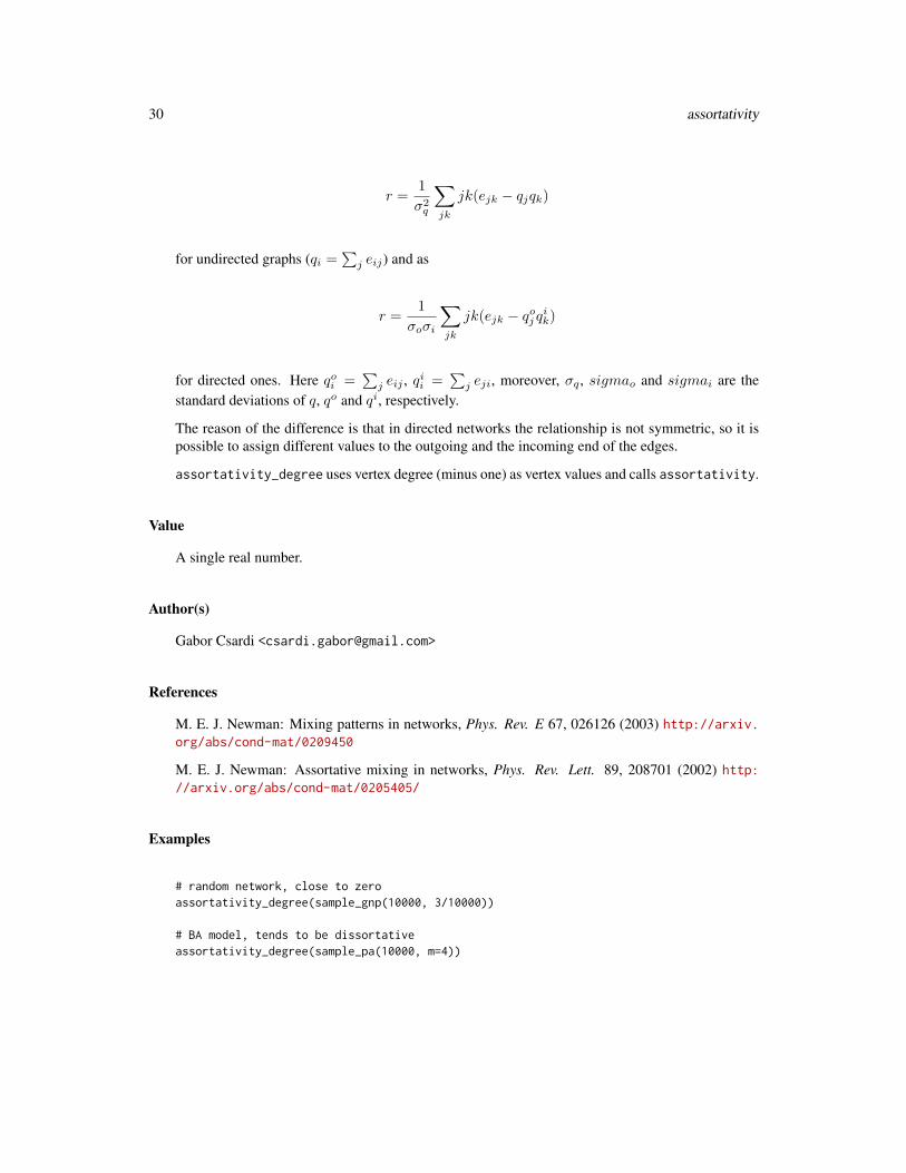
30 assortativity
r =1
σ2q
∑jk
jk(ejk − qjqk)
for undirected graphs (qi =∑j eij) and as
r =1
σoσi
∑jk
jk(ejk − qoj qik)
for directed ones. Here qoi =∑j eij , q
ii =
∑j eji, moreover, σq , sigmao and sigmai are the
standard deviations of q, qo and qi, respectively.
The reason of the difference is that in directed networks the relationship is not symmetric, so it ispossible to assign different values to the outgoing and the incoming end of the edges.
assortativity_degree uses vertex degree (minus one) as vertex values and calls assortativity.
Value
A single real number.
Author(s)
Gabor Csardi <[email protected]>
References
M. E. J. Newman: Mixing patterns in networks, Phys. Rev. E 67, 026126 (2003) http://arxiv.org/abs/cond-mat/0209450
M. E. J. Newman: Assortative mixing in networks, Phys. Rev. Lett. 89, 208701 (2002) http://arxiv.org/abs/cond-mat/0205405/
Examples
# random network, close to zeroassortativity_degree(sample_gnp(10000, 3/10000))
# BA model, tends to be dissortativeassortativity_degree(sample_pa(10000, m=4))

as_adjacency_matrix 31
as_adjacency_matrix Convert a graph to an adjacency matrix
Description
Sometimes it is useful to work with a standard representation of a graph, like an adjacency matrix.
Usage
as_adjacency_matrix(graph, type = c("both", "upper", "lower"), attr = NULL,edges = FALSE, names = TRUE, sparse = igraph_opt("sparsematrices"))
as_adj(graph, type = c("both", "upper", "lower"), attr = NULL,edges = FALSE, names = TRUE, sparse = igraph_opt("sparsematrices"))
Arguments
graph The graph to convert.
type Gives how to create the adjacency matrix for undirected graphs. It is ignored fordirected graphs. Possible values: upper: the upper right triangle of the matrixis used, lower: the lower left triangle of the matrix is used. both: the wholematrix is used, a symmetric matrix is returned.
attr Either NULL or a character string giving an edge attribute name. If NULL a tra-ditional adjacency matrix is returned. If not NULL then the values of the givenedge attribute are included in the adjacency matrix. If the graph has multipleedges, the edge attribute of an arbitrarily chosen edge (for the multiple edges) isincluded. This argument is ignored if edges is TRUE.Note that this works only for certain attribute types. If the sparse argumenis TRUE, then the attribute must be either logical or numeric. If the sparseargument is FALSE, then character is also allowed. The reason for the differenceis that the Matrix package does not support character sparse matrices yet.
edges Logical scalar, whether to return the edge ids in the matrix. For non-existantedges zero is returned.
names Logical constant, whether to assign row and column names to the matrix. Theseare only assigned if the name vertex attribute is present in the graph.
sparse Logical scalar, whether to create a sparse matrix. The ‘Matrix’ package mustbe installed for creating sparse matrices.
Details
as_adjacency_matrix returns the adjacency matrix of a graph, a regular matrix if sparse is FALSE,or a sparse matrix, as defined in the ‘Matrix’ package, if sparse if TRUE.
Value
A vcount(graph) by vcount(graph) (usually) numeric matrix.

32 as_adj_list
See Also
graph_from_adjacency_matrix, read_graph
Examples
g <- sample_gnp(10, 2/10)as_adjacency_matrix(g)V(g)$name <- letters[1:vcount(g)]as_adjacency_matrix(g)E(g)$weight <- runif(ecount(g))as_adjacency_matrix(g, attr="weight")
as_adj_list Adjacency lists
Description
Create adjacency lists from a graph, either for adjacent edges or for neighboring vertices
Usage
as_adj_list(graph, mode = c("all", "out", "in", "total"))
as_adj_edge_list(graph, mode = c("all", "out", "in", "total"))
Arguments
graph The input graph.
mode Character scalar, it gives what kind of adjacent edges/vertices to include in thelists. ‘out’ is for outgoing edges/vertices, ‘in’ is for incoming edges/vertices,‘all’ is for both. This argument is ignored for undirected graphs.
Details
as_adj_list returns a list of numeric vectors, which include the ids of neighbor vertices (accordingto the mode argument) of all vertices.
as_adj_edge_list returns a list of numeric vectors, which include the ids of adjacent edgs (ac-cording to the mode argument) of all vertices.
Value
A list of numeric vectors.
Author(s)
Gabor Csardi <[email protected]>
as_data_frame 33
See Also
as_edgelist, as_adj
Examples
g <- make_ring(10)as_adj_list(g)as_adj_edge_list(g)
as_data_frame Creating igraph graphs from data frames or vice-versa
Description
This function creates an igraph graph from one or two data frames containing the (symbolic) edgelist and edge/vertex attributes.
Usage
as_data_frame(x, what = c("edges", "vertices", "both"))
graph_from_data_frame(d, directed = TRUE, vertices = NULL)
from_data_frame(...)
Arguments
x An igraph object.
what Character constant, whether to return info about vertices, edges, or both. Thedefault is ‘edges’.
d A data frame containing a symbolic edge list in the first two columns. Additionalcolumns are considered as edge attributes. Since version 0.7 this argument iscoerced to a data frame with as.data.frame.
directed Logical scalar, whether or not to create a directed graph.
vertices A data frame with vertex metadata, or NULL. See details below. Since version0.7 this argument is coerced to a data frame with as.data.frame, if not NULL.
... Passed to graph_from_data_frame.

34 as_data_frame
Details
graph_from_data_frame creates igraph graphs from one or two data frames. It has two modes ofoperatation, depending whether the vertices argument is NULL or not.
If vertices is NULL, then the first two columns of d are used as a symbolic edge list and additionalcolumns as edge attributes. The names of the attributes are taken from the names of the columns.
If vertices is not NULL, then it must be a data frame giving vertex metadata. The first columnof vertices is assumed to contain symbolic vertex names, this will be added to the graphs as the‘name’ vertex attribute. Other columns will be added as additional vertex attributes. If verticesis not NULL then the symbolic edge list given in d is checked to contain only vertex names listed invertices.
Typically, the data frames are exported from some speadsheat software like Excel and are importedinto R via read.table, read.delim or read.csv.
as_data_frame converts the igraph graph into one or more data frames, depending on the whatargument.
If the what argument is edges (the default), then the edges of the graph and also the edge attributesare returned. The edges will be in the first two columns, named from and to. (This also denotesedge direction for directed graphs.) For named graphs, the vertex names will be included in thesecolumns, for other graphs, the numeric vertex ids. The edge attributes will be in the other columns.It is not a good idea to have an edge attribute named from or to, because then the column named inthe data frame will not be unique. The edges are listed in the order of their numeric ids.
If the what argument is vertices, then vertex attributes are returned. Vertices are listed in the orderof their numeric vertex ids.
If the what argument is both, then both vertex and edge data is returned, in a list with named entriesvertices and edges.
Value
An igraph graph object for graph_from_data_frame, and either a data frame or a list of two dataframes named edges and vertices for as.data.frame.
Note
For graph_from_data_frame NA elements in the first two columns ‘d’ are replaced by the string“NA” before creating the graph. This means that all NAs will correspond to a single vertex.
NA elements in the first column of ‘vertices’ are also replaced by the string “NA”, but the rest of‘vertices’ is not touched. In other words, vertex names (=the first column) cannot be NA, but othervertex attributes can.
Author(s)
Gabor Csardi <[email protected]>
See Also
graph_from_literal for another way to create graphs, read.table to read in tables from files.
as_edgelist 35
Examples
## A simple example with a couple of actors## The typical case is that these tables are read in from files....actors <- data.frame(name=c("Alice", "Bob", "Cecil", "David",
"Esmeralda"),age=c(48,33,45,34,21),gender=c("F","M","F","M","F"))
relations <- data.frame(from=c("Bob", "Cecil", "Cecil", "David","David", "Esmeralda"),
to=c("Alice", "Bob", "Alice", "Alice", "Bob", "Alice"),same.dept=c(FALSE,FALSE,TRUE,FALSE,FALSE,TRUE),friendship=c(4,5,5,2,1,1), advice=c(4,5,5,4,2,3))
g <- graph_from_data_frame(relations, directed=TRUE, vertices=actors)print(g, e=TRUE, v=TRUE)
## The opposite operationas_data_frame(g, what="vertices")as_data_frame(g, what="edges")
as_edgelist Convert a graph to an edge list
Description
Sometimes it is useful to work with a standard representation of a graph, like an edge list.
Usage
as_edgelist(graph, names = TRUE)
Arguments
graph The graph to convert.
names Whether to return a character matrix containing vertex names (ie. the namevertex attribute) if they exist or numeric vertex ids.
Details
as_edgelist returns the list of edges in a graph.
Value
A gsize(graph) by 2 numeric matrix.
See Also
graph_from_adjacency_matrix, read_graph

36 as_graphnel
Examples
g <- sample_gnp(10, 2/10)as_edgelist(g)
V(g)$name <- LETTERS[seq_len(gorder(g))]as_edgelist(g)
as_graphnel Convert igraph graphs to graphNEL objects from the graph package
Description
The graphNEL class is defined in the graph package, it is another way to represent graphs. Thesefunctions are provided to convert between the igraph and the graphNEL objects.
Usage
as_graphnel(graph)
Arguments
graph An igraph graph object.
Details
as_graphnel converts an igraph graph to a graphNEL graph. It converts all graph/vertex/edgeattributes. If the igraph graph has a vertex attribute ‘name’, then it will be used to assign vertexnames in the graphNEL graph. Otherwise numeric igraph vertex ids will be used for this purpose.
Value
as_graphnel returns a graphNEL graph object.
See Also
graph_from_graphnel for the other direction, as_adj, graph_from_adjacency_matrix, as_adj_listand graph.adjlist for other graph representations.
Examples
## Undirected## Not run:g <- make_ring(10)V(g)$name <- letters[1:10]GNEL <- as_graphnel(g)g2 <- graph_from_graphnel(GNEL)g2
as_ids 37
## Directedg3 <- make_star(10, mode="in")V(g3)$name <- letters[1:10]GNEL2 <- as_graphnel(g3)g4 <- graph_from_graphnel(GNEL2)g4
## End(Not run)
as_ids Convert a vertex or edge sequence to an ordinary vector
Description
Convert a vertex or edge sequence to an ordinary vector
Usage
as_ids(seq)
## S3 method for class 'igraph.vs'as_ids(seq)
## S3 method for class 'igraph.es'as_ids(seq)
Arguments
seq The vertex or edge sequence.
Details
For graphs without names, a numeric vector is returned, containing the internal numeric vertex oredge ids.
For graphs with names, and vertex sequences, the vertex names are returned in a character vector.
For graphs with names and edge sequences, a character vector is returned, with the ‘bar’ notation:a|b means an edge from vertex a to vertex b.
Value
A character or numeric vector, see details below.

38 as_incidence_matrix
Examples
g <- make_ring(10)as_ids(V(g))as_ids(E(g))
V(g)$name <- letters[1:10]as_ids(V(g))as_ids(E(g))
as_incidence_matrix Incidence matrix of a bipartite graph
Description
This function can return a sparse or dense incidence matrix of a bipartite network. The incidencematrix is an n times m matrix, n and m are the number of vertices of the two kinds.
Usage
as_incidence_matrix(graph, types = NULL, attr = NULL, names = TRUE,sparse = FALSE)
Arguments
graph The input graph. The direction of the edges is ignored in directed graphs.
types An optional vertex type vector to use instead of the type vertex attribute. Youmust supply this argument if the graph has no type vertex attribute.
attr Either NULL or a character string giving an edge attribute name. If NULL, then atraditional incidence matrix is returned. If not NULL then the values of the givenedge attribute are included in the incidence matrix. If the graph has multipleedges, the edge attribute of an arbitrarily chosen edge (for the multiple edges) isincluded.
names Logical scalar, if TRUE and the vertices in the graph are named (i.e. the graphhas a vertex attribute called name), then vertex names will be added to the resultas row and column names. Otherwise the ids of the vertices are used as row andcolumn names.
sparse Logical scalar, if it is TRUE then a sparse matrix is created, you will need theMatrix package for this.
Details
Bipartite graphs have a type vertex attribute in igraph, this is boolean and FALSE for the vertices ofthe first kind and TRUE for vertices of the second kind.
Value
A sparse or dense matrix.

as_long_data_frame 39
Author(s)
Gabor Csardi <[email protected]>
See Also
graph_from_incidence_matrix for the opposite operation.
Examples
g <- make_bipartite_graph( c(0,1,0,1,0,0), c(1,2,2,3,3,4) )as_incidence_matrix(g)
as_long_data_frame Convert a graph to a long data frame
Description
A long data frame contains all metadata about both the vertices and edges of the graph. It containsone row for each edge, and all metadata about that edge and its incident vertices are included in thatrow. The names of the columns that contain the metadata of the incident vertices are prefixed withfrom_ and to_. The first two columns are always named from and to and they contain the numericids of the incident vertices. The rows are listed in the order of numeric vertex ids.
Usage
as_long_data_frame(graph)
Arguments
graph Input graph
Value
A long data frame.
Examples
g <- make_(ring(10),with_vertex_(name = letters[1:10], color = "red"),with_edge_(weight = 1:10, color = "green")
)as_long_data_frame(g)

40 authority_score
as_membership Declare a numeric vector as a membership vector
Description
This is useful if you want to use functions defined on membership vectors, but your membershipvector does not come from an igraph clustering method.
Usage
as_membership(x)
Arguments
x The input vector.
Value
The input vector, with the membership class added.
Examples
## Compare to the correct clusteringg <- (make_full_graph(10) + make_full_graph(10)) %>%
rewire(each_edge(p = 0.2))correct <- rep(1:2, each = 10) %>% as_membershipfc <- cluster_fast_greedy(g)compare(correct, fc)compare(correct, membership(fc))
authority_score Kleinberg’s authority centrality scores.
Description
The authority scores of the vertices are defined as the principal eigenvector of ATA, where A is theadjacency matrix of the graph.
Usage
authority_score(graph, scale = TRUE, weights = NULL,options = arpack_defaults)
authority_score 41
Arguments
graph The input graph.
scale Logical scalar, whether to scale the result to have a maximum score of one. Ifno scaling is used then the result vector has unit length in the Euclidean norm.
weights Optional positive weight vector for calculating weighted scores. If the graphhas a weight edge attribute, then this is used by default. This function interpretsedge weights as connection strengths. In the random surfer model, an edge witha larger weight is more likely to be selected by the surfer.
options A named list, to override some ARPACK options. See arpack for details.
Details
For undirected matrices the adjacency matrix is symmetric and the authority scores are the same ashub scores, see hub_score.
Value
A named list with members:
vector The authority/hub scores of the vertices.
value The corresponding eigenvalue of the calculated principal eigenvector.
options Some information about the ARPACK computation, it has the same members asthe options member returned by arpack, see that for documentation.
References
J. Kleinberg. Authoritative sources in a hyperlinked environment. Proc. 9th ACM-SIAM Symposiumon Discrete Algorithms, 1998. Extended version in Journal of the ACM 46(1999). Also appears asIBM Research Report RJ 10076, May 1997.
See Also
hub_score, eigen_centrality for eigenvector centrality, page_rank for the Page Rank scores.arpack for the underlining machinery of the computation.
Examples
## An in-starg <- make_star(10)hub_score(g)$vectorauthority_score(g)$vector
## A ringg2 <- make_ring(10)hub_score(g2)$vectorauthority_score(g2)$vector

42 automorphisms
automorphisms Number of automorphisms
Description
Calculate the number of automorphisms of a graph, i.e. the number of isomorphisms to itself.
Usage
automorphisms(graph, sh = "fm")
Arguments
graph The input graph, it is treated as undirected.
sh The splitting heuristics for the BLISS algorithm. Possible values are: ‘f’: firstnon-singleton cell, ‘fl’: first largest non-singleton cell, ‘fs’: first smallest non-singleton cell, ‘fm’: first maximally non-trivially connected non-singleton cell,‘flm’: first largest maximally non-trivially connected non-singleton cell, ‘fsm’:first smallest maximally non-trivially connected non-singleton cell.
Details
An automorphism of a graph is a permutation of its vertices which brings the graph into itself.
This function calculates the number of automorphism of a graph using the BLISS algorithm. Seealso the BLISS homepage at http://www.tcs.hut.fi/Software/bliss/index.html.
Value
A named list with the following members:
group_size The size of the automorphism group of the input graph, as a string. This numberis exact if igraph was compiled with the GMP library, and approximate other-wise.
nof_nodes The number of nodes in the search tree.
nof_leaf_nodes The number of leaf nodes in the search tree.
nof_bad_nodes Number of bad nodes.
nof_canupdates Number of canrep updates.
max_level Maximum level.
Author(s)
Tommi Junttila (http://users.ics.aalto.fi/tjunttil/) for BLISS and Gabor Csardi <[email protected]>for the igraph glue code and this manual page.

bfs 43
References
Tommi Junttila and Petteri Kaski: Engineering an Efficient Canonical Labeling Tool for Large andSparse Graphs, Proceedings of the Ninth Workshop on Algorithm Engineering and Experiments andthe Fourth Workshop on Analytic Algorithms and Combinatorics. 2007.
See Also
canonical_permutation, permute
Examples
## A ring has n*2 automorphisms, you can "turn" it by 0-9 vertices## and each of these graphs can be "flipped"g <- make_ring(10)automorphisms(g)
bfs Breadth-first search
Description
Breadth-first search is an algorithm to traverse a graph. We start from a root vertex and spread alongevery edge “simultaneously”.
Usage
bfs(graph, root, neimode = c("out", "in", "all", "total"),unreachable = TRUE, restricted = NULL, order = TRUE, rank = FALSE,father = FALSE, pred = FALSE, succ = FALSE, dist = FALSE,callback = NULL, extra = NULL, rho = parent.frame())
Arguments
graph The input graph.
root Numeric vector, usually of length one. The root vertex, or root vertices to startthe search from.
neimode For directed graphs specifies the type of edges to follow. ‘out’ follows outgo-ing, ‘in’ incoming edges. ‘all’ ignores edge directions completely. ‘total’ is asynonym for ‘all’. This argument is ignored for undirected graphs.
unreachable Logical scalar, whether the search should visit the vertices that are unreachablefrom the given root vertex (or vertices). If TRUE, then additional searches areperformed until all vertices are visited.
restricted NULL (=no restriction), or a vector of vertices (ids or symbolic names). In thelatter case, the search is restricted to the given vertices.
order Logical scalar, whether to return the ordering of the vertices.

44 bfs
rank Logical scalar, whether to return the rank of the vertices.
father Logical scalar, whether to return the father of the vertices.
pred Logical scalar, whether to return the predecessors of the vertices.
succ Logical scalar, whether to return the successors of the vertices.
dist Logical scalar, whether to return the distance from the root of the search tree.
callback If not NULL, then it must be callback function. This is called whenever a vertexis visited. See details below.
extra Additional argument to supply to the callback function.
rho The environment in which the callback function is evaluated.
Details
The callback function must have the following arguments:
graph The input graph is passed to the callback function here.
data A named numeric vector, with the following entries: ‘vid’, the vertex that was just visited,‘pred’, its predecessor, ‘succ’, its successor, ‘rank’, the rank of the current vertex, ‘dist’, itsdistance from the root of the search tree.
extra The extra argument.
See examples below on how to use the callback function.
Value
A named list with the following entries:
root Numeric scalar. The root vertex that was used as the starting point of the search.
neimode Character scalar. The neimode argument of the function call. Note that forundirected graphs this is always ‘all’, irrespectively of the supplied value.
order Numeric vector. The vertex ids, in the order in which they were visited by thesearch.
rank Numeric vector. The rank for each vertex.
father Numeric vector. The father of each vertex, i.e. the vertex it was discovered from.
pred Numeric vector. The previously visited vertex for each vertex, or 0 if there wasno such vertex.
succ Numeric vector. The next vertex that was visited after the current one, or 0 ifthere was no such vertex.
dist Numeric vector, for each vertex its distance from the root of the search tree.
Note that order, rank, father, pred, succ and dist might be NULL if their corresponding argumentis FALSE, i.e. if their calculation is not requested.
Author(s)
Gabor Csardi <[email protected]>

biconnected_components 45
See Also
dfs for depth-first search.
Examples
## Two ringsbfs(make_ring(10) %du% make_ring(10), root=1, "out",
order=TRUE, rank=TRUE, father=TRUE, pred=TRUE,succ=TRUE, dist=TRUE)
## How to use a callbackf <- function(graph, data, extra) {
print(data)FALSE
}tmp <- bfs(make_ring(10) %du% make_ring(10), root=1, "out",
callback=f)
## How to use a callback to stop the search## We stop after visiting all vertices in the initial componentf <- function(graph, data, extra) {data['succ'] == -1
}bfs(make_ring(10) %du% make_ring(10), root=1, callback=f)
biconnected_components
Biconnected components
Description
Finding the biconnected components of a graph
Usage
biconnected_components(graph)
Arguments
graph The input graph. It is treated as an undirected graph, even if it is directed.

46 biconnected_components
Details
A graph is biconnected if the removal of any single vertex (and its adjacent edges) does not discon-nect it.
A biconnected component of a graph is a maximal biconnected subgraph of it. The biconnectedcomponents of a graph can be given by the partition of its edges: every edge is a member of exactlyone biconnected component. Note that this is not true for vertices: the same vertex can be part ofmany biconnected components.
Value
A named list with three components:
no Numeric scalar, an integer giving the number of biconnected components in thegraph.
tree_edges The components themselves, a list of numeric vectors. Each vector is a set ofedge ids giving the edges in a biconnected component. These edges define aspanning tree of the component.
component_edges
A list of numeric vectors. It gives all edges in the components.
components A list of numeric vectors, the vertices of the components.
articulation_points
The articulation points of the graph. See articulation_points.
Author(s)
Gabor Csardi <[email protected]>
See Also
articulation_points, components, is_connected, vertex_connectivity
Examples
g <- disjoint_union( make_full_graph(5), make_full_graph(5) )clu <- components(g)$membershipg <- add_edges(g, c(which(clu==1), which(clu==2)))bc <- biconnected_components(g)

bipartite_mapping 47
bipartite_mapping Decide whether a graph is bipartite
Description
This function decides whether the vertices of a network can be mapped to two vertex types in a waythat no vertices of the same type are connected.
Usage
bipartite_mapping(graph)
Arguments
graph The input graph.
Details
A bipartite graph in igraph has a ‘type’ vertex attribute giving the two vertex types.
This function simply checks whether a graph could be bipartite. It tries to find a mapping that givesa possible division of the vertices into two classes, such that no two vertices of the same class areconnected by an edge.
The existence of such a mapping is equivalent of having no circuits of odd length in the graph. Agraph with loop edges cannot bipartite.
Note that the mapping is not necessarily unique, e.g. if the graph has at least two components, thenthe vertices in the separate components can be mapped independently.
Value
A named list with two elements:
res A logical scalar, TRUE if the can be bipartite, FALSE otherwise.
type A possibly vertex type mapping, a logical vector. If no such mapping exists,then an empty vector.
Author(s)
Gabor Csardi <[email protected]>
Examples
## A ring has just one loop, so it is fineg <- make_ring(10)bipartite_mapping(g)
## A star is fine, too

48 bipartite_projection
g2 <- make_star(10)bipartite_mapping(g2)
## A graph containing a triangle is not fineg3 <- make_ring(10)g3 <- add_edges(g3, c(1,3))bipartite_mapping(g3)
bipartite_projection Project a bipartite graph
Description
A bipartite graph is projected into two one-mode networks
Usage
bipartite_projection(graph, types = NULL, multiplicity = TRUE,probe1 = NULL, which = c("both", "true", "false"), remove.type = TRUE)
Arguments
graph The input graph. It can be directed, but edge directions are ignored during thecomputation.
types An optional vertex type vector to use instead of the ‘type’ vertex attribute. Youmust supply this argument if the graph has no ‘type’ vertex attribute.
multiplicity If TRUE, then igraph keeps the multiplicity of the edges as an edge attribute called‘weight’. E.g. if there is an A-C-B and also an A-D-B triple in the bipartite graph(but no more X, such that A-X-B is also in the graph), then the multiplicity ofthe A-B edge in the projection will be 2.
probe1 This argument can be used to specify the order of the projections in the resultinglist. If given, then it is considered as a vertex id (or a symbolic vertex name);the projection containing this vertex will be the first one in the result list. Thisargument is ignored if only one projection is requested in argument which.
which A character scalar to specify which projection(s) to calculate. The default is tocalculate both.
remove.type Logical scalar, whether to remove the type vertex attribute from the projections.This makes sense because these graphs are not bipartite any more. However ifyou want to combine them with each other (or other bipartite graphs), then it isworth keeping this attribute. By default it will be removed.

c.igraph.es 49
Details
Bipartite graphs have a type vertex attribute in igraph, this is boolean and FALSE for the vertices ofthe first kind and TRUE for vertices of the second kind.
bipartite_projection_size calculates the number of vertices and edges in the two projectionsof the bipartite graphs, without calculating the projections themselves. This is useful to check howmuch memory the projections would need if you have a large bipartite graph.
bipartite_projection calculates the actual projections. You can use the probe1 argument tospecify the order of the projections in the result. By default vertex type FALSE is the first and TRUEis the second.
bipartite_projection keeps vertex attributes.
Value
A list of two undirected graphs. See details above.
Author(s)
Gabor Csardi <[email protected]>
Examples
## Projection of a full bipartite graph is a full graphg <- make_full_bipartite_graph(10,5)proj <- bipartite_projection(g)graph.isomorphic(proj[[1]], make_full_graph(10))graph.isomorphic(proj[[2]], make_full_graph(5))
## The projection keeps the vertex attributesM <- matrix(0, nr=5, nc=3)rownames(M) <- c("Alice", "Bob", "Cecil", "Dan", "Ethel")colnames(M) <- c("Party", "Skiing", "Badminton")M[] <- sample(0:1, length(M), replace=TRUE)Mg2 <- graph_from_incidence_matrix(M)g2$name <- "Event network"proj2 <- bipartite_projection(g2)print(proj2[[1]], g=TRUE, e=TRUE)print(proj2[[2]], g=TRUE, e=TRUE)
c.igraph.es Concatenate edge sequences
Description
Concatenate edge sequences

50 c.igraph.vs
Usage
## S3 method for class 'igraph.es'c(..., recursive = FALSE)
Arguments
... The edge sequences to concatenate. They must all refer to the same graph.
recursive Ignored, included for S3 compatibility with the base c function.
Value
An edge sequence, the input sequences concatenated.
See Also
Other vertex and edge sequence operations: c.igraph.vs, difference.igraph.es, difference.igraph.vs,igraph-es-indexing2, igraph-es-indexing, igraph-vs-indexing2, igraph-vs-indexing, intersection.igraph.es,intersection.igraph.vs, rev.igraph.es, rev.igraph.vs, union.igraph.es, union.igraph.vs,unique.igraph.es, unique.igraph.vs
Examples
g <- make_(ring(10), with_vertex_(name = LETTERS[1:10]))c(E(g)[1], E(g)['A|B'], E(g)[1:4])
c.igraph.vs Concatenate vertex sequences
Description
Concatenate vertex sequences
Usage
## S3 method for class 'igraph.vs'c(..., recursive = FALSE)
Arguments
... The vertex sequences to concatenate. They must refer to the same graph.
recursive Ignored, included for S3 compatibility with the base c function.
Value
A vertex sequence, the input sequences concatenated.
canonical_permutation 51
See Also
Other vertex and edge sequence operations: c.igraph.es, difference.igraph.es, difference.igraph.vs,igraph-es-indexing2, igraph-es-indexing, igraph-vs-indexing2, igraph-vs-indexing, intersection.igraph.es,intersection.igraph.vs, rev.igraph.es, rev.igraph.vs, union.igraph.es, union.igraph.vs,unique.igraph.es, unique.igraph.vs
Examples
g <- make_(ring(10), with_vertex_(name = LETTERS[1:10]))c(V(g)[1], V(g)['A'], V(g)[1:4])
canonical_permutation Canonical permutation of a graph
Description
The canonical permutation brings every isomorphic graphs into the same (labeled) graph.
Usage
canonical_permutation(graph, sh = "fm")
Arguments
graph The input graph, treated as undirected.
sh Type of the heuristics to use for the BLISS algorithm. See details for possiblevalues.
Details
canonical_permutation computes a permutation which brings the graph into canonical form, asdefined by the BLISS algorithm. All isomorphic graphs have the same canonical form.
See the paper below for the details about BLISS. This and more information is available at http://www.tcs.hut.fi/Software/bliss/index.html.
The possible values for the sh argument are:
"f" First non-singleton cell.
"fl" First largest non-singleton cell.
"fs" First smallest non-singleton cell.
"fm" First maximally non-trivially connectec non-singleton cell.
"flm" Largest maximally non-trivially connected non-singleton cell.
"fsm" Smallest maximally non-trivially connected non-singleton cell.
See the paper in references for details about these.

52 canonical_permutation
Value
A list with the following members:
labeling The canonical parmutation which takes the input graph into canonical form. Anumeric vector, the first element is the new label of vertex 0, the second elementfor vertex 1, etc.
info Some information about the BLISS computation. A named list with the follow-ing members:
"nof_nodes" The number of nodes in the search tree."nof_leaf_nodes" The number of leaf nodes in the search tree."nof_bad_nodes" Number of bad nodes."nof_canupdates" Number of canrep updates."max_level" Maximum level."group_size" The size of the automorphism group of the input graph, as a
string. This number is exact if igraph was compiled with the GMP library,and approximate otherwise.
Author(s)
Tommi Junttila for BLISS, Gabor Csardi <[email protected]> for the igraph and R inter-faces.
References
Tommi Junttila and Petteri Kaski: Engineering an Efficient Canonical Labeling Tool for Large andSparse Graphs, Proceedings of the Ninth Workshop on Algorithm Engineering and Experiments andthe Fourth Workshop on Analytic Algorithms and Combinatorics. 2007.
See Also
permute to apply a permutation to a graph, graph.isomorphic for deciding graph isomorphism,possibly based on canonical labels.
Examples
## Calculate the canonical form of a random graphg1 <- sample_gnm(10, 20)cp1 <- canonical_permutation(g1)cf1 <- permute(g1, cp1$labeling)
## Do the same with a random permutation of itg2 <- permute(g1, sample(vcount(g1)))cp2 <- canonical_permutation(g2)cf2 <- permute(g2, cp2$labeling)
## Check that they are the sameel1 <- as_edgelist(cf1)el2 <- as_edgelist(cf2)

categorical_pal 53
el1 <- el1[ order(el1[,1], el1[,2]), ]el2 <- el2[ order(el2[,1], el2[,2]), ]all(el1 == el2)
categorical_pal Palette for categories
Description
This is a color blind friendly palette from http://jfly.iam.u-tokyo.ac.jp/color. It has 8colors.
Usage
categorical_pal(n)
Arguments
n The number of colors in the palette. We simply take the first n colors from thetotal 8.
Details
This is the suggested palette for visualizations where vertex colors mark categories, e.g. communitymembership.
Value
A character vector of RGB color codes.
Examples
library(igraphdata)data(karate)karate <- karate
add_layout_(with_fr())set_vertex_attr("size", value = 10)
cl_k <- cluster_optimal(karate)
V(karate)$color <- membership(cl_k)karate$palette <- categorical_pal(length(cl_k))plot(karate)
See Also
Other palettes: diverging_pal, r_pal, sequential_pal

54 centralize
centralize Centralization of a graph
Description
Centralization is a method for creating a graph level centralization measure from the centralityscores of the vertices.
Usage
centralize(scores, theoretical.max = 0, normalized = TRUE)
Arguments
scores The vertex level centrality scores.theoretical.max
Real scalar. The graph level centrality score of the most centralized graph withthe same number of vertices as the graph under study. This is only used if thenormalized argument is set to TRUE.
normalized Logical scalar. Whether to normalize the graph level centrality score by dividingby the supplied theoretical maximum.
Details
Centralization is a general method for calculating a graph-level centrality score based on node-levelcentrality measure. The formula for this is
C(G) =∑v
(maxw
cw − cv),
where cv is the centrality of vertex v.
The graph-level centrality score can be normalized by dividing by the maximum theoretical scorefor a graph with the same number of vertices, using the same parameters, e.g. directedness, whetherwe consider loop edges, etc.
For degree, closeness and betweenness the most centralized structure is some version of the stargraph, in-star, out-star or undirected star.
For eigenvector centrality the most centralized structure is the graph with a single edge (and poten-tially many isolates).
centralize implements general centralization formula to calculate a graph-level score from vertex-level scores.
Value
A real scalar, the centralization of the graph from which scores were derived.
centr_betw 55
References
Freeman, L.C. (1979). Centrality in Social Networks I: Conceptual Clarification. Social Networks1, 215–239.
Wasserman, S., and Faust, K. (1994). Social Network Analysis: Methods and Applications. Cam-bridge University Press.
See Also
Other centralization related: centr_betw_tmax, centr_betw, centr_clo_tmax, centr_clo, centr_degree_tmax,centr_degree, centr_eigen_tmax, centr_eigen
Examples
# A BA graph is quite centralizedg <- sample_pa(1000, m=4)centr_degree(g)$centralizationcentr_clo(g, mode="all")$centralizationcentr_eigen(g, directed=FALSE)$centralization
# The most centralized graph according to eigenvector centralityg0 <- graph( c(2,1), n=10, dir=FALSE )g1 <- make_star(10, mode="undirected")centr_eigen(g0)$centralizationcentr_eigen(g1)$centralization
centr_betw Centralize a graph according to the betweenness of vertices
Description
See centralize for a summary of graph centralization.
Usage
centr_betw(graph, directed = TRUE, nobigint = TRUE, normalized = TRUE)
Arguments
graph The input graph.
directed logical scalar, whether to use directed shortest paths for calculating between-ness.
nobigint Logical scalar, whether to use big integers for the betweenness calculation. Thisargument is passed to the betweenness function.
normalized Logical scalar. Whether to normalize the graph level centrality score by dividingby the theoretical maximum.

56 centr_betw_tmax
Value
A named list with the following components:
res The node-level centrality scores.
centralization The graph level centrality index.theoretical_max
The maximum theoretical graph level centralization score for a graph with thegiven number of vertices, using the same parameters. If the normalized argu-ment was TRUE, then the result was divided by this number.
See Also
Other centralization related: centr_betw_tmax, centr_clo_tmax, centr_clo, centr_degree_tmax,centr_degree, centr_eigen_tmax, centr_eigen, centralize
Examples
# A BA graph is quite centralizedg <- sample_pa(1000, m = 4)centr_degree(g)$centralizationcentr_clo(g, mode = "all")$centralizationcentr_betw(g, directed = FALSE)$centralizationcentr_eigen(g, directed = FALSE)$centralization
centr_betw_tmax Theoretical maximum for betweenness centralization
Description
See centralize for a summary of graph centralization.
Usage
centr_betw_tmax(graph = NULL, nodes = 0, directed = TRUE)
Arguments
graph The input graph. It can also be NULL, if nodes is given.
nodes The number of vertices. This is ignored if the graph is given.
directed logical scalar, whether to use directed shortest paths for calculating between-ness.
Value
Real scalar, the theoratical maximum (unnormalized) graph betweenness centrality score for graphswith given order and other parameters.

centr_clo 57
See Also
Other centralization related: centr_betw, centr_clo_tmax, centr_clo, centr_degree_tmax,centr_degree, centr_eigen_tmax, centr_eigen, centralize
Examples
# A BA graph is quite centralizedg <- sample_pa(1000, m = 4)centr_betw(g, normalized = FALSE)$centralization %>%`/`(centr_betw_tmax(g))
centr_betw(g, normalized = TRUE)$centralization
centr_clo Centralize a graph according to the closeness of vertices
Description
See centralize for a summary of graph centralization.
Usage
centr_clo(graph, mode = c("out", "in", "all", "total"), normalized = TRUE)
Arguments
graph The input graph.
mode This is the same as the mode argument of closeness.
normalized Logical scalar. Whether to normalize the graph level centrality score by dividingby the theoretical maximum.
Value
A named list with the following components:
res The node-level centrality scores.
centralization The graph level centrality index.theoretical_max
The maximum theoretical graph level centralization score for a graph with thegiven number of vertices, using the same parameters. If the normalized argu-ment was TRUE, then the result was divided by this number.
See Also
Other centralization related: centr_betw_tmax, centr_betw, centr_clo_tmax, centr_degree_tmax,centr_degree, centr_eigen_tmax, centr_eigen, centralize

58 centr_clo_tmax
Examples
# A BA graph is quite centralizedg <- sample_pa(1000, m = 4)centr_degree(g)$centralizationcentr_clo(g, mode = "all")$centralizationcentr_betw(g, directed = FALSE)$centralizationcentr_eigen(g, directed = FALSE)$centralization
centr_clo_tmax Theoretical maximum for closeness centralization
Description
See centralize for a summary of graph centralization.
Usage
centr_clo_tmax(graph = NULL, nodes = 0, mode = c("out", "in", "all","total"))
Arguments
graph The input graph. It can also be NULL, if nodes is given.
nodes The number of vertices. This is ignored if the graph is given.
mode This is the same as the mode argument of closeness.
Value
Real scalar, the theoratical maximum (unnormalized) graph closeness centrality score for graphswith given order and other parameters.
See Also
Other centralization related: centr_betw_tmax, centr_betw, centr_clo, centr_degree_tmax,centr_degree, centr_eigen_tmax, centr_eigen, centralize
Examples
# A BA graph is quite centralizedg <- sample_pa(1000, m = 4)centr_clo(g, normalized = FALSE)$centralization %>%`/`(centr_clo_tmax(g))
centr_clo(g, normalized = TRUE)$centralization

centr_degree 59
centr_degree Centralize a graph according to the degrees of vertices
Description
See centralize for a summary of graph centralization.
Usage
centr_degree(graph, mode = c("all", "out", "in", "total"), loops = TRUE,normalized = TRUE)
Arguments
graph The input graph.
mode This is the same as the mode argument of degree.
loops Logical scalar, whether to consider loops edges when calculating the degree.
normalized Logical scalar. Whether to normalize the graph level centrality score by dividingby the theoretical maximum.
Value
A named list with the following components:
res The node-level centrality scores.
centralization The graph level centrality index.theoretical_max
The maximum theoretical graph level centralization score for a graph with thegiven number of vertices, using the same parameters. If the normalized argu-ment was TRUE, then the result was divided by this number.
See Also
Other centralization related: centr_betw_tmax, centr_betw, centr_clo_tmax, centr_clo, centr_degree_tmax,centr_eigen_tmax, centr_eigen, centralize
Examples
# A BA graph is quite centralizedg <- sample_pa(1000, m = 4)centr_degree(g)$centralizationcentr_clo(g, mode = "all")$centralizationcentr_betw(g, directed = FALSE)$centralizationcentr_eigen(g, directed = FALSE)$centralization

60 centr_degree_tmax
centr_degree_tmax Theoretical maximum for degree centralization
Description
See centralize for a summary of graph centralization.
Usage
centr_degree_tmax(graph = NULL, nodes = 0, mode = c("all", "out", "in","total"), loops = FALSE)
Arguments
graph The input graph. It can also be NULL, if nodes, mode and loops are all given.
nodes The number of vertices. This is ignored if the graph is given.
mode This is the same as the mode argument of degree.
loops Logical scalar, whether to consider loops edges when calculating the degree.
Value
Real scalar, the theoratical maximum (unnormalized) graph degree centrality score for graphs withgiven order and other parameters.
See Also
Other centralization related: centr_betw_tmax, centr_betw, centr_clo_tmax, centr_clo, centr_degree,centr_eigen_tmax, centr_eigen, centralize
Examples
# A BA graph is quite centralizedg <- sample_pa(1000, m = 4)centr_degree(g, normalized = FALSE)$centralization %>%`/`(centr_degree_tmax(g))centr_degree(g, normalized = TRUE)$centralization

centr_eigen 61
centr_eigen Centralize a graph according to the eigenvector centrality of vertices
Description
See centralize for a summary of graph centralization.
Usage
centr_eigen(graph, directed = FALSE, scale = TRUE,options = arpack_defaults, normalized = TRUE)
Arguments
graph The input graph.
directed logical scalar, whether to use directed shortest paths for calculating eigenvectorcentrality.
scale Whether to rescale the eigenvector centrality scores, such that the maximumscore is one.
options This is passed to eigen_centrality, the options for the ARPACK eigensolver.
normalized Logical scalar. Whether to normalize the graph level centrality score by dividingby the theoretical maximum.
Value
A named list with the following components:
vector The node-level centrality scores.
value The corresponding eigenvalue.
options ARPACK options, see the return value of eigen_centrality for details.
centralization The graph level centrality index.
theoretical_max
The same as above, the theoretical maximum centralization score for a graphwith the same number of vertices.
See Also
Other centralization related: centr_betw_tmax, centr_betw, centr_clo_tmax, centr_clo, centr_degree_tmax,centr_degree, centr_eigen_tmax, centralize

62 centr_eigen_tmax
Examples
# A BA graph is quite centralizedg <- sample_pa(1000, m = 4)centr_degree(g)$centralizationcentr_clo(g, mode = "all")$centralizationcentr_betw(g, directed = FALSE)$centralizationcentr_eigen(g, directed = FALSE)$centralization
# The most centralized graph according to eigenvector centralityg0 <- make_graph(c(2,1), n = 10, dir = FALSE)g1 <- make_star(10, mode = "undirected")centr_eigen(g0)$centralizationcentr_eigen(g1)$centralization
centr_eigen_tmax Theoretical maximum for betweenness centralization
Description
See centralize for a summary of graph centralization.
Usage
centr_eigen_tmax(graph = NULL, nodes = 0, directed = FALSE,scale = TRUE)
Arguments
graph The input graph. It can also be NULL, if nodes is given.
nodes The number of vertices. This is ignored if the graph is given.
directed logical scalar, whether to use directed shortest paths for calculating between-ness.
scale Whether to rescale the eigenvector centrality scores, such that the maximumscore is one.
Value
Real scalar, the theoratical maximum (unnormalized) graph betweenness centrality score for graphswith given order and other parameters.
See Also
Other centralization related: centr_betw_tmax, centr_betw, centr_clo_tmax, centr_clo, centr_degree_tmax,centr_degree, centr_eigen, centralize

cliques 63
Examples
# A BA graph is quite centralizedg <- sample_pa(1000, m = 4)centr_eigen(g, normalized = FALSE)$centralization %>%`/`(centr_eigen_tmax(g))
centr_eigen(g, normalized = TRUE)$centralization
cliques The functions find cliques, ie. complete subgraphs in a graph
Description
These functions find all, the largest or all the maximal cliques in an undirected graph. The size ofthe largest clique can also be calculated.
Usage
cliques(graph, min = NULL, max = NULL)
max_cliques(graph, min = NULL, max = NULL, subset = NULL, file = NULL)
Arguments
graph The input graph, directed graphs will be considered as undirected ones, multipleedges and loops are ignored.
min Numeric constant, lower limit on the size of the cliques to find. NULL means nolimit, ie. it is the same as 0.
max Numeric constant, upper limit on the size of the cliques to find. NULL means nolimit.
subset If not NULL, then it must be a vector of vertex ids, numeric or symbolic if thegraph is named. The algorithm is run from these vertices only, so only a subsetof all maximal cliques is returned. See the Eppstein paper for details. Thisargument makes it possible to easily parallelize the finding of maximal cliques.
file If not NULL, then it must be a file name, i.e. a character scalar. The output of thealgorithm is written to this file. (If it exists, then it will be overwritten.) Eachclique will be a separate line in the file, given with the numeric ids of its vertices,separated by whitespace.
Details
cliques find all complete subgraphs in the input graph, obeying the size limitations given in themin and max arguments.
largest_cliques finds all largest cliques in the input graph. A clique is largest if there is no otherclique including more vertices.

64 cliques
max_cliques finds all maximal cliques in the input graph. A clique in maximal if it cannot beextended to a larger clique. The largest cliques are always maximal, but a maximal clique is notneccessarily the largest.
count_max_cliques counts the maximal cliques.
clique_num calculates the size of the largest clique(s).
The current implementation of these functions searches for maximal independent vertex sets (seeivs) in the complementer graph.
Value
cliques, largest_cliques and clique_num return a list containing numeric vectors of vertex ids.Each list element is a clique.
max_cliques returns NULL, invisibly, if its file argument is not NULL. The output is written to thespecified file in this case.
clique_num and count_max_cliques return an integer scalar.
Author(s)
Tamas Nepusz <[email protected]> and Gabor Csardi <[email protected]>
References
For maximal cliques the following algorithm is implemented: David Eppstein, Maarten Loffler,Darren Strash: Listing All Maximal Cliques in Sparse Graphs in Near-optimal Time. http://arxiv.org/abs/1006.5440
See Also
ivs
Examples
# this usually contains cliques of size sixg <- sample_gnp(100, 0.3)clique_num(g)cliques(g, min=6)largest_cliques(g)
# To have a bit less maximal cliques, about 100-200 usuallyg <- sample_gnp(100, 0.03)max_cliques(g)
closeness 65
closeness Closeness centrality of vertices
Description
Cloness centrality measures how many steps is required to access every other vertex from a givenvertex.
Usage
closeness(graph, vids = V(graph), mode = c("out", "in", "all", "total"),weights = NULL, normalized = FALSE)
estimate_closeness(graph, vids = V(graph), mode = c("out", "in", "all","total"), cutoff, weights = NULL, normalized = FALSE)
Arguments
graph The graph to analyze.
vids The vertices for which closeness will be calculated.
mode Character string, defined the types of the paths used for measuring the distancein directed graphs. “in” measures the paths to a vertex, “out” measures pathsfrom a vertex, all uses undirected paths. This argument is ignored for undirectedgraphs.
weights Optional positive weight vector for calculating weighted closeness. If the graphhas a weight edge attribute, then this is used by default. Weights are used forcalculating weighted shortest paths, so they are interpreted as distances.
normalized Logical scalar, whether to calculate the normalized closeness. Normalization isperformed by multiplying the raw closeness by n− 1, where n is the number ofvertices in the graph.
cutoff The maximum path length to consider when calculating the betweenness. If zeroor negative then there is no such limit.
Details
The closeness centrality of a vertex is defined by the inverse of the average length of the shortestpaths to/from all the other vertices in the graph:
1∑i 6=v dvi
If there is no (directed) path between vertex v and i then the total number of vertices is used in theformula instead of the path length.
estimate_closeness only considers paths of length cutoff or smaller, this can be run for largergraphs, as the running time is not quadratic (if cutoff is small). If cutoff is zero or negative thenthe function calculates the exact closeness scores.

66 cluster_edge_betweenness
Value
Numeric vector with the closeness values of all the vertices in v.
Author(s)
Gabor Csardi <[email protected]>
References
Freeman, L.C. (1979). Centrality in Social Networks I: Conceptual Clarification. Social Networks,1, 215-239.
See Also
betweenness, degree
Examples
g <- make_ring(10)g2 <- make_star(10)closeness(g)closeness(g2, mode="in")closeness(g2, mode="out")closeness(g2, mode="all")
cluster_edge_betweenness
Community structure detection based on edge betweenness
Description
Many networks consist of modules which are densely connected themselves but sparsely connectedto other modules.
Usage
cluster_edge_betweenness(graph, weights = E(graph)$weight, directed = TRUE,edge.betweenness = TRUE, merges = TRUE, bridges = TRUE,modularity = TRUE, membership = TRUE)

cluster_edge_betweenness 67
Arguments
graph The graph to analyze.
weights The edge weights. Supply NULL to omit edge weights. By default the ‘weight’edge attribute is used, if it is present. Edge weights are used to calculate weightededge betweenness. This means that edges are interpreted as distances, not asconnection strengths.
directed Logical constant, whether to calculate directed edge betweenness for directedgraphs. It is ignored for undirected graphs.
edge.betweenness
Logical constant, whether to return the edge betweenness of the edges at thetime of their removal.
merges Logical constant, whether to return the merge matrix representing the hierarchi-cal community structure of the network. This argument is called merges, evenif the community structure algorithm itself is divisive and not agglomerative: itbuilds the tree from top to bottom. There is one line for each merge (i.e. split) inmatrix, the first line is the first merge (last split). The communities are identifiedby integer number starting from one. Community ids smaller than or equal toN , the number of vertices in the graph, belong to singleton communities, ie.individual vertices. Before the first merge we have N communities numberedfrom one to N . The first merge, the first line of the matrix creates communityN + 1, the second merge creates community N + 2, etc.
bridges Logical constant, whether to return a list the edge removals which actually split-ted a component of the graph.
modularity Logical constant, whether to calculate the maximum modularity score, consid-ering all possibly community structures along the edge-betweenness based edgeremovals.
membership Logical constant, whether to calculate the membership vector corresponding tothe highest possible modularity score.
Details
The edge betweenness score of an edge measures the number of shortest paths through it, seeedge_betweenness for details. The idea of the edge betweenness based community structure de-tection is that it is likely that edges connecting separate modules have high edge betweenness asall the shortest paths from one module to another must traverse through them. So if we graduallyremove the edge with the highest edge betweenness score we will get a hierarchical map, a rootedtree, called a dendrogram of the graph. The leafs of the tree are the individual vertices and the rootof the tree represents the whole graph.
cluster_edge_betweenness performs this algorithm by calculating the edge betweenness of thegraph, removing the edge with the highest edge betweenness score, then recalculating edge be-tweenness of the edges and again removing the one with the highest score, etc.
edge.betweeness.community returns various information collected throught the run of the algo-rithm. See the return value down here.

68 cluster_fast_greedy
Value
cluster_edge_betweenness returns a communities object, please see the communities manualpage for details.
Author(s)
Gabor Csardi <[email protected]>
References
M Newman and M Girvan: Finding and evaluating community structure in networks, PhysicalReview E 69, 026113 (2004)
See Also
edge_betweenness for the definition and calculation of the edge betweenness, cluster_walktrap,cluster_fast_greedy, cluster_leading_eigen for other community detection methods.
See communities for extracting the results of the community detection.
Examples
g <- sample_pa(100, m = 2, directed = FALSE)eb <- cluster_edge_betweenness(g)
g <- make_full_graph(10) %du% make_full_graph(10)g <- add_edges(g, c(1,11))eb <- cluster_edge_betweenness(g)eb
cluster_fast_greedy Community structure via greedy optimization of modularity
Description
This function tries to find dense subgraph, also called communities in graphs via directly optimizinga modularity score.
Usage
cluster_fast_greedy(graph, merges = TRUE, modularity = TRUE,membership = TRUE, weights = E(graph)$weight)

cluster_fast_greedy 69
Arguments
graph The input graphmerges Logical scalar, whether to return the merge matrix.modularity Logical scalar, whether to return a vector containing the modularity after each
merge.membership Logical scalar, whether to calculate the membership vector corresponding to
the maximum modularity score, considering all possible community structuresalong the merges.
weights If not NULL, then a numeric vector of edge weights. The length must match thenumber of edges in the graph. By default the ‘weight’ edge attribute is usedas weights. If it is not present, then all edges are considered to have the sameweight. Larger edge weights correspond to stronger connections.
Details
This function implements the fast greedy modularity optimization algorithm for finding communitystructure, see A Clauset, MEJ Newman, C Moore: Finding community structure in very largenetworks, http://www.arxiv.org/abs/cond-mat/0408187 for the details.
Value
cluster_fast_greedy returns a communities object, please see the communities manual pagefor details.
Author(s)
Tamas Nepusz <[email protected]> and Gabor Csardi <[email protected]> for the Rinterface.
References
A Clauset, MEJ Newman, C Moore: Finding community structure in very large networks, http://www.arxiv.org/abs/cond-mat/0408187
See Also
communities for extracting the results.
See also cluster_walktrap, cluster_spinglass, cluster_leading_eigen and cluster_edge_betweennessfor other methods.
Examples
g <- make_full_graph(5) %du% make_full_graph(5) %du% make_full_graph(5)g <- add_edges(g, c(1,6, 1,11, 6, 11))fc <- cluster_fast_greedy(g)membership(fc)sizes(fc)

70 cluster_infomap
cluster_infomap Infomap community finding
Description
Find community structure that minimizes the expected description length of a random walker tra-jectory
Usage
cluster_infomap(graph, e.weights = NULL, v.weights = NULL, nb.trials = 10,modularity = TRUE)
Arguments
graph The input graph.
e.weights If not NULL, then a numeric vector of edge weights. The length must match thenumber of edges in the graph. By default the ‘weight’ edge attribute is usedas weights. If it is not present, then all edges are considered to have the sameweight. Larger edge weights correspond to stronger connections.
v.weights If not NULL, then a numeric vector of vertex weights. The length must match thenumber of vertices in the graph. By default the ‘weight’ vertex attribute is usedas weights. If it is not present, then all vertices are considered to have the sameweight. A larger vertex weight means a larger probability that the random surferjumps to that vertex.
nb.trials The number of attempts to partition the network (can be any integer value equalor larger than 1).
modularity Logical scalar, whether to calculate the modularity score of the detected com-munity structure.
Details
Please see the details of this method in the references given below.
Value
cluster_infomap returns a communities object, please see the communities manual page fordetails.
Author(s)
Martin Rosvall (http://www.tp.umu.se/~rosvall/) wrote the original C++ code. This wasported to be more igraph-like by Emmanuel Navarro. The R interface and some cosmetics wasdone by Gabor Csardi <[email protected]>.

cluster_label_prop 71
References
The original paper: M. Rosvall and C. T. Bergstrom, Maps of information flow reveal commu-nity structure in complex networks, PNAS 105, 1118 (2008) http://dx.doi.org/10.1073/pnas.0706851105, http://arxiv.org/abs/0707.0609
A more detailed paper: M. Rosvall, D. Axelsson, and C. T. Bergstrom, The map equation, Eur.Phys. J. Special Topics 178, 13 (2009). http://dx.doi.org/10.1140/epjst/e2010-01179-1,http://arxiv.org/abs/0906.1405.
See Also
Other community finding methods and communities.
Examples
## Zachary's karate clubg <- make_graph("Zachary")
imc <- cluster_infomap(g)membership(imc)communities(imc)
cluster_label_prop Finding communities based on propagating labels
Description
This is a fast, nearly linear time algorithm for detecting community structure in networks. In worksby labeling the vertices with unique labels and then updating the labels by majority voting in theneighborhood of the vertex.
Usage
cluster_label_prop(graph, weights = NULL, initial = NULL, fixed = NULL)
Arguments
graph The input graph, should be undirected to make sense.
weights An optional weight vector. It should contain a positive weight for all the edges.The ‘weight’ edge attribute is used if present. Supply ‘NA’ here if you want toignore the ‘weight’ edge attribute. Larger edge weights correspond to strongerconnections.
initial The initial state. If NULL, every vertex will have a different label at the beginning.Otherwise it must be a vector with an entry for each vertex. Non-negative valuesdenote different labels, negative entries denote vertices without labels.

72 cluster_label_prop
fixed Logical vector denoting which labels are fixed. Of course this makes sense onlyif you provided an initial state, otherwise this element will be ignored. Also notethat vertices without labels cannot be fixed.
Details
This function implements the community detection method described in: Raghavan, U.N. and Al-bert, R. and Kumara, S.: Near linear time algorithm to detect community structures in large-scalenetworks. Phys Rev E 76, 036106. (2007). This version extends the original method by the abilityto take edge weights into consideration and also by allowing some labels to be fixed.
From the abstract of the paper: “In our algorithm every node is initialized with a unique labeland at every step each node adopts the label that most of its neighbors currently have. In thisiterative process densely connected groups of nodes form a consensus on a unique label to formcommunities.”
Value
cluster_label_prop returns a communities object, please see the communities manual page fordetails.
Author(s)
Tamas Nepusz <[email protected]> for the C implementation, Gabor Csardi <[email protected]>for this manual page.
References
Raghavan, U.N. and Albert, R. and Kumara, S.: Near linear time algorithm to detect communitystructures in large-scale networks. Phys Rev E 76, 036106. (2007)
See Also
communities for extracting the actual results.
cluster_fast_greedy, cluster_walktrap and cluster_spinglass for other community detec-tion methods.
Examples
g <- sample_gnp(10, 5/10) %du% sample_gnp(9, 5/9)g <- add_edges(g, c(1, 12))cluster_label_prop(g)

cluster_leading_eigen 73
cluster_leading_eigen Community structure detecting based on the leading eigenvector of thecommunity matrix
Description
This function tries to find densely connected subgraphs in a graph by calculating the leading non-negative eigenvector of the modularity matrix of the graph.
Usage
cluster_leading_eigen(graph, steps = -1, weights = NULL, start = NULL,options = arpack_defaults, callback = NULL, extra = NULL,env = parent.frame())
Arguments
graph The input graph. Should be undirected as the method needs a symmetric matrix.steps The number of steps to take, this is actually the number of tries to make a step.
It is not a particularly useful parameter.weights An optional weight vector. The ‘weight’ edge attribute is used if present. Supply
‘NA’ here if you want to ignore the ‘weight’ edge attribute. Larger edge weightscorrespond to stronger connections between vertices.
start NULL, or a numeric membership vector, giving the start configuration of the al-gorithm.
options A named list to override some ARPACK options.callback If not NULL, then it must be callback function. This is called after each iteration,
after calculating the leading eigenvector of the modularity matrix. See detailsbelow.
extra Additional argument to supply to the callback function.env The environment in which the callback function is evaluated.
Details
The function documented in these section implements the ‘leading eigenvector’ method developedby Mark Newman, see the reference below.
The heart of the method is the definition of the modularity matrix, B, which is B=A-P, A beingthe adjacency matrix of the (undirected) network, and P contains the probability that certain edgesare present according to the ‘configuration model’. In other words, a P[i,j] element of P is theprobability that there is an edge between vertices i and j in a random network in which the degreesof all vertices are the same as in the input graph.
The leading eigenvector method works by calculating the eigenvector of the modularity matrix forthe largest positive eigenvalue and then separating vertices into two community based on the signof the corresponding element in the eigenvector. If all elements in the eigenvector are of the samesign that means that the network has no underlying comuunity structure. Check Newman’s paper tounderstand why this is a good method for detecting community structure.

74 cluster_leading_eigen
Value
cluster_leading_eigen returns a named list with the following members:
membership The membership vector at the end of the algorithm, when no more splits arepossible.
merges The merges matrix starting from the state described by the membership member.This is a two-column matrix and each line describes a merge of two communi-ties, the first line is the first merge and it creates community ‘N’, N is the numberof initial communities in the graph, the second line creates community N+1, etc.
options Information about the underlying ARPACK computation, see arpack for details.
Callback functions
The callback argument can be used to supply a function that is called after each eigenvectorcalculation. The following arguments are supplied to this function:
membership The actual membership vector, with zero-based indexing.
community The community that the algorithm just tried to split, community numbering starts withzero here.
value The eigenvalue belonging to the leading eigenvector the algorithm just found.
vector The leading eigenvector the algorithm just found.
multiplier An R function that can be used to multiple the actual modularity matrix with an arbitraryvector. Supply the vector as an argument to perform this multiplication. This function can beused with ARPACK.
extra The extra argument that was passed to cluster_leading_eigen. The callback functionshould return a scalar number. If this number is non-zero, then the clustering is terminated.
Author(s)
Gabor Csardi <[email protected]>
References
MEJ Newman: Finding community structure using the eigenvectors of matrices, Physical ReviewE 74 036104, 2006.
See Also
modularity, cluster_walktrap, cluster_edge_betweenness, cluster_fast_greedy, as.dendrogram
Examples
g <- make_full_graph(5) %du% make_full_graph(5) %du% make_full_graph(5)g <- add_edges(g, c(1,6, 1,11, 6, 11))lec <- cluster_leading_eigen(g)lec

cluster_louvain 75
cluster_leading_eigen(g, start=membership(lec))
cluster_louvain Finding community structure by multi-level optimization of modularity
Description
This function implements the multi-level modularity optimization algorithm for finding communitystructure, see references below. It is based on the modularity measure and a hierarchial approach.
Usage
cluster_louvain(graph, weights = NULL)
Arguments
graph The input graph.
weights Optional positive weight vector. If the graph has a weight edge attribute, thenthis is used by default. Supply NA here if the graph has a weight edge attribute,but you want to ignore it. Larger edge weights correspond to stronger connec-tions.
Details
This function implements the multi-level modularity optimization algorithm for finding communitystructure, see VD Blondel, J-L Guillaume, R Lambiotte and E Lefebvre: Fast unfolding of commu-nity hierarchies in large networks, http://arxiv.org/abs/arXiv:0803.0476 for the details.
It is based on the modularity measure and a hierarchial approach. Initially, each vertex is assignedto a community on its own. In every step, vertices are re-assigned to communities in a local, greedyway: each vertex is moved to the community with which it achieves the highest contribution tomodularity. When no vertices can be reassigned, each community is considered a vertex on its own,and the process starts again with the merged communities. The process stops when there is only asingle vertex left or when the modularity cannot be increased any more in a step.
This function was contributed by Tom Gregorovic.
Value
cluster_louvain returns a communities object, please see the communities manual page fordetails.
Author(s)
Tom Gregorovic, Tamas Nepusz <[email protected]>

76 cluster_optimal
References
Vincent D. Blondel, Jean-Loup Guillaume, Renaud Lambiotte, Etienne Lefebvre: Fast unfolding ofcommunities in large networks. J. Stat. Mech. (2008) P10008
See Also
See communities for extracting the membership, modularity scores, etc. from the results.
Other community detection algorithms: cluster_walktrap, cluster_spinglass, cluster_leading_eigen,cluster_edge_betweenness, cluster_fast_greedy, cluster_label_prop
Examples
# This is so simple that we will have only one levelg <- make_full_graph(5) %du% make_full_graph(5) %du% make_full_graph(5)g <- add_edges(g, c(1,6, 1,11, 6, 11))cluster_louvain(g)
cluster_optimal Optimal community structure
Description
This function calculates the optimal community structure of a graph, by maximizing the modularitymeasure over all possible partitions.
Usage
cluster_optimal(graph, weights = NULL)
Arguments
graph The input graph. Edge directions are ignored for directed graphs.
weights Optional positive weight vector for optimizing weighted modularity. If the graphhas a weight edge attribute, then this is used by default. Supply NA to ignorethe weights of a weighted graph. Larger edge weights correspond to strongerconnections.
Details
This function calculates the optimal community structure for a graph, in terms of maximal modu-larity score.
The calculation is done by transforming the modularity maximization into an integer programmingproblem, and then calling the GLPK library to solve that. Please the reference below for details.
Note that modularity optimization is an NP-complete problem, and all known algorithms for it haveexponential time complexity. This means that you probably don’t want to run this function on larger

cluster_optimal 77
graphs. Graphs with up to fifty vertices should be fine, graphs with a couple of hundred verticesmight be possible.
Value
cluster_optimal returns a communities object, please see the communities manual page fordetails.
Examples
## Zachary's karate clubg <- make_graph("Zachary")
## We put everything into a big 'try' block, in case## igraph was compiled without GLPK support
## The calculation only takes a couple of secondsoc <- cluster_optimal(g)
## Double check the resultprint(modularity(oc))print(modularity(g, membership(oc)))
## Compare to the greedy optimizerfc <- cluster_fast_greedy(g)print(modularity(fc))
Author(s)
Gabor Csardi <[email protected]>
References
Ulrik Brandes, Daniel Delling, Marco Gaertler, Robert Gorke, Martin Hoefer, Zoran Nikoloski,Dorothea Wagner: On Modularity Clustering, IEEE Transactions on Knowledge and Data Engi-neering 20(2):172-188, 2008.
See Also
communities for the documentation of the result, modularity. See also cluster_fast_greedyfor a fast greedy optimizer.

78 cluster_spinglass
cluster_spinglass Finding communities in graphs based on statistical meachanics
Description
This function tries to find communities in graphs via a spin-glass model and simulated annealing.
Usage
cluster_spinglass(graph, weights = NULL, vertex = NULL, spins = 25,parupdate = FALSE, start.temp = 1, stop.temp = 0.01, cool.fact = 0.99,update.rule = c("config", "random", "simple"), gamma = 1,implementation = c("orig", "neg"), gamma.minus = 1)
Arguments
graph The input graph, can be directed but the direction of the edges is neglected.
weights The weights of the edges. Either a numeric vector or NULL. If it is null and theinput graph has a ‘weight’ edge attribute then that will be used. If NULL andno such attribute is present then the edges will have equal weights. Set this toNA if the graph was a ‘weight’ edge attribute, but you don’t want to use it forcommunity detection. A larger edge weight means a stronger connection forthis function.
vertex This parameter can be used to calculate the community of a given vertex withoutcalculating all communities. Note that if this argument is present then someother arguments are ignored.
spins Integer constant, the number of spins to use. This is the upper limit for thenumber of communities. It is not a problem to supply a (reasonably) big numberhere, in which case some spin states will be unpopulated.
parupdate Logical constant, whether to update the spins of the vertices in parallel (syn-chronously) or not. This argument is ignored if the second form of the functionis used (ie. the ‘vertex’ argument is present). It is also not implemented in the“neg” implementation.
start.temp Real constant, the start temperature. This argument is ignored if the second formof the function is used (ie. the ‘vertex’ argument is present).
stop.temp Real constant, the stop temperature. The simulation terminates if the tempera-ture lowers below this level. This argument is ignored if the second form of thefunction is used (ie. the ‘vertex’ argument is present).
cool.fact Cooling factor for the simulated annealing. This argument is ignored if thesecond form of the function is used (ie. the ‘vertex’ argument is present).
update.rule Character constant giving the ‘null-model’ of the simulation. Possible values:“simple” and “config”. “simple” uses a random graph with the same numberof edges as the baseline probability and “config” uses a random graph with thesame vertex degrees as the input graph.

cluster_spinglass 79
gamma Real constant, the gamma argument of the algorithm. This specifies the bal-ance between the importance of present and non-present edges in a community.Roughly, a comunity is a set of vertices having many edges inside the commu-nity and few edges outside the community. The default 1.0 value makes exist-ing and non-existing links equally important. Smaller values make the existinglinks, greater values the missing links more important.
implementation Character scalar. Currently igraph contains two implementations for the Spin-glass community finding algorithm. The faster original implementation is thedefault. The other implementation, that takes into account negative weights, canbe chosen by supplying ‘neg’ here.
gamma.minus Real constant, the gamma.minus parameter of the algorithm. This specifies thebalance between the importance of present and non-present negative weightededges in a community. Smaller values of gamma.minus, leads to communitieswith lesser negative intra-connectivity. If this argument is set to zero, the al-gorithm reduces to a graph coloring algorithm, using the number of spins asthe number of colors. This argument is ignored if the ‘orig’ implementation ischosen.
Details
This function tries to find communities in a graph. A community is a set of nodes with many edgesinside the community and few edges between outside it (i.e. between the community itself and therest of the graph.)
This idea is reversed for edges having a negative weight, ie. few negative edges inside a communityand many negative edges between communities. Note that only the ‘neg’ implementation supportsnegative edge weights.
The spinglass.cummunity function can solve two problems related to community detection. Ifthe vertex argument is not given (or it is NULL), then the regular community detection problem issolved (approximately), i.e. partitioning the vertices into communities, by optimizing the an energyfunction.
If the vertex argument is given and it is not NULL, then it must be a vertex id, and the same energyfunction is used to find the community of the the given vertex. See also the examples below.
Value
If the vertex argument is not given, ie. the first form is used then a cluster_spinglass returns acommunities object.
If the vertex argument is present, ie. the second form is used then a named list is returned with thefollowing components:
community Numeric vector giving the ids of the vertices in the same community as vertex.
cohesion The cohesion score of the result, see references.
adhesion The adhesion score of the result, see references.
inner.links The number of edges within the community of vertex.
outer.links The number of edges between the community of vertex and the rest of thegraph.

80 cluster_walktrap
Author(s)
Jorg Reichardt for the original code and Gabor Csardi <[email protected]> for the igraphglue code.
Changes to the original function for including the possibility of negative ties were implemented byVincent Traag (http://www.traag.net/).
References
J. Reichardt and S. Bornholdt: Statistical Mechanics of Community Detection, Phys. Rev. E, 74,016110 (2006), http://arxiv.org/abs/cond-mat/0603718
M. E. J. Newman and M. Girvan: Finding and evaluating community structure in networks, Phys.Rev. E 69, 026113 (2004)
V.A. Traag and Jeroen Bruggeman: Community detection in networks with positive and negativelinks, http://arxiv.org/abs/0811.2329 (2008).
See Also
communities, components
Examples
g <- sample_gnp(10, 5/10) %du% sample_gnp(9, 5/9)g <- add_edges(g, c(1, 12))g <- induced_subgraph(g, subcomponent(g, 1))cluster_spinglass(g, spins=2)cluster_spinglass(g, vertex=1)
cluster_walktrap Community strucure via short random walks
Description
This function tries to find densely connected subgraphs, also called communities in a graph viarandom walks. The idea is that short random walks tend to stay in the same community.
Usage
cluster_walktrap(graph, weights = E(graph)$weight, steps = 4,merges = TRUE, modularity = TRUE, membership = TRUE)

cluster_walktrap 81
Arguments
graph The input graph, edge directions are ignored in directed graphs.
weights The edge weights. Larger edge weights increase the probability that an edge isselected by the random walker. In other words, larger edge weights correspondto stronger connections.
steps The length of the random walks to perform.
merges Logical scalar, whether to include the merge matrix in the result.
modularity Logical scalar, whether to include the vector of the modularity scores in theresult. If the membership argument is true, then it will be always calculated.
membership Logical scalar, whether to calculate the membership vector for the split corre-sponding to the highest modularity value.
Details
This function is the implementation of the Walktrap community finding algorithm, see Pascal Pons,Matthieu Latapy: Computing communities in large networks using random walks, http://arxiv.org/abs/physics/0512106
Value
cluster_walktrap returns a communities object, please see the communities manual page fordetails.
Author(s)
Pascal Pons (http://psl.pons.free.fr/) and Gabor Csardi <[email protected]> forthe R and igraph interface
References
Pascal Pons, Matthieu Latapy: Computing communities in large networks using random walks,http://arxiv.org/abs/physics/0512106
See Also
See communities on getting the actual membership vector, merge matrix, modularity score, etc.
modularity and cluster_fast_greedy, cluster_spinglass, cluster_leading_eigen, cluster_edge_betweennessfor other community detection methods.
Examples
g <- make_full_graph(5) %du% make_full_graph(5) %du% make_full_graph(5)g <- add_edges(g, c(1,6, 1,11, 6, 11))cluster_walktrap(g)

82 cocitation
cocitation Cocitation coupling
Description
Two vertices are cocited if there is another vertex citing both of them. cocitation siply countshow many types two vertices are cocited. The bibliographic coupling of two vertices is the numberof other vertices they both cite, bibcoupling calculates this.
Usage
cocitation(graph, v = V(graph))
Arguments
graph The graph object to analyze
v Vertex sequence or numeric vector, the vertex ids for which the cocitation orbibliographic coupling values we want to calculate. The default is all vertices.
Details
cocitation calculates the cocitation counts for the vertices in the v argument and all vertices inthe graph.
bibcoupling calculates the bibliographic coupling for vertices in v and all vertices in the graph.
Calculating the cocitation or bibliographic coupling for only one vertex costs the same amount ofcomputation as for all vertices. This might change in the future.
Value
A numeric matrix with length(v) lines and vcount(graph) columns. Element (i,j) contains thecocitation or bibliographic coupling for vertices v[i] and j.
Author(s)
Gabor Csardi <[email protected]>
Examples
g <- make_ring(10)cocitation(g)bibcoupling(g)

cohesive_blocks 83
cohesive_blocks Calculate Cohesive Blocks
Description
Calculates cohesive blocks for objects of class igraph.
Usage
cohesive_blocks(graph, labels = TRUE)
## S3 method for class 'cohesiveBlocks'length(x)
blocks(blocks)
graphs_from_cohesive_blocks(blocks, graph)
## S3 method for class 'cohesiveBlocks'cohesion(x, ...)
hierarchy(blocks)
parent(blocks)
## S3 method for class 'cohesiveBlocks'print(x, ...)
## S3 method for class 'cohesiveBlocks'summary(object, ...)
## S3 method for class 'cohesiveBlocks'plot(x, y, colbar = rainbow(max(cohesion(x)) + 1),col = colbar[max_cohesion(x) + 1], mark.groups = blocks(x)[-1], ...)
plot_hierarchy(blocks, layout = layout_as_tree(hierarchy(blocks), root = 1),...)
export_pajek(blocks, graph, file, project.file = TRUE)
max_cohesion(blocks)
Arguments
graph For cohesive_blocks a graph object of class igraph. It must be undirectedand simple. (See is_simple.)

84 cohesive_blocks
For graphs_from_cohesive_blocks and export_pajek the same graph mustbe supplied whose cohesive block structure is given in the blocks argument.
labels Logical scalar, whether to add the vertex labels to the result object. These labelscan be then used when reporting and plotting the cohesive blocks.
blocks, x, object
A cohesiveBlocks object, created with the cohesive_blocks function.
... Additional arguments. plot_hierarchy and plot pass them to plot.igraph.print and summary ignore them.
y The graph whose cohesive blocks are supplied in the x argument.
colbar Color bar for the vertex colors. Its length should be at least m + 1, where m isthe maximum cohesion in the graph. Alternatively, the vertex colors can also bedirectly specified via the col argument.
col A vector of vertex colors, in any of the usual formats. (Symbolic color names(e.g. ‘red’, ‘blue’, etc.) , RGB colors (e.g. ‘#FF9900FF’), integer numbersreferring to the current palette. By default the given colbar is used and verticeswith the same maximal cohesion will have the same color.
mark.groups A list of vertex sets to mark on the plot by circling them. By default all cohesiveblocks are marked, except the one corresponding to the all vertices.
layout The layout of a plot, it is simply passed on to plot.igraph, see the possibleformats there. By default the Reingold-Tilford layout generator is used.
file Defines the file (or connection) the Pajek file is written to.If the project.file argument is TRUE, then it can be a filename (with exten-sion), a file object, or in general any king of connection object. The file/connectionwill be opened if it wasn’t already.If the project.file argument is FALSE, then several files are created and filemust be a character scalar containing the base name of the files, without exten-sion. (But it can contain the path to the files.)See also details below.
project.file Logical scalar, whether to create a single Pajek project file containing all thedata, or to create separated files for each item. See details below.
Details
Cohesive blocking is a method of determining hierarchical subsets of graph vertices based on theirstructural cohesion (or vertex connectivity). For a given graph G, a subset of its vertices S ⊂ V (G)is said to be maximally k-cohesive if there is no superset of S with vertex connectivity greater thanor equal to k. Cohesive blocking is a process through which, given a k-cohesive set of vertices,maximally l-cohesive subsets are recursively identified with l > k. Thus a hiearchy of vertexsubsets is found, whith the entire graph G at its root.
The function cohesive_blocks implements cohesive blocking. It returns a cohesiveBlocks ob-ject. cohesiveBlocks should be handled as an opaque class, i.e. its internal structure should not beaccessed directly, but through the functions listed here.
The function length can be used on cohesiveBlocks objects and it gives the number of blocks.
The function blocks returns the actual blocks stored in the cohesiveBlocks object. They arereturned in a list of numeric vectors, each containing vertex ids.

cohesive_blocks 85
The function graphs_from_cohesive_blocks is similar, but returns the blocks as (induced) sub-graphs of the input graph. The various (graph, vertex and edge) attributes are kept in the subgraph.
The function cohesion returns a numeric vector, the cohesion of the different blocks. The order ofthe blocks is the same as for the blocks and graphs_from_cohesive_blocks functions.
The block hierarchy can be queried using the hierarchy function. It returns an igraph graph, its ver-tex ids are ordered according the order of the blocks in the blocks and graphs_from_cohesive_blocks,cohesion, etc. functions.
parent gives the parent vertex of each block, in the block hierarchy, for the root vertex it gives 0.
plot_hierarchy plots the hierarchy tree of the cohesive blocks on the active graphics device, bycalling igraph.plot.
The export_pajek function can be used to export the graph and its cohesive blocks in Pajek format.It can either export a single Pajek project file with all the information, or a set of files, depending onits project.file argument. If project.file is TRUE, then the following information is written tothe file (or connection) given in the file argument: (1) the input graph, together with its attributes,see write_graph for details; (2) the hierarchy graph; and (3) one binary partition for each cohesiveblock. If project.file is FALSE, then the file argument must be a character scalar and it is usedas the base name for the generated files. If file is ‘basename’, then the following files are created:(1) ‘basename.net’ for the original graph; (2) ‘basename_hierarchy.net’ for the hierarchy graph; (3)‘basename_block_x.net’ for each cohesive block, where ‘x’ is the number of the block, starting withone.
max_cohesion returns the maximal cohesion of each vertex, i.e. the cohesion of the most cohesiveblock of the vertex.
The generic function summary works on cohesiveBlocks objects and it prints a one line summaryto the terminal.
The generic function print is also defined on cohesiveBlocks objects and it is invoked automati-cally if the name of the cohesiveBlocks object is typed in. It produces an output like this:
Cohesive block structure:B-1 c 1, n 23'- B-2 c 2, n 14 oooooooo.. .o......oo ooo'- B-4 c 5, n 7 ooooooo... .......... ...'- B-3 c 2, n 10 ......o.oo o.oooooo.. ...'- B-5 c 3, n 4 ......o.oo o......... ...
The left part shows the block structure, in this case for five blocks. The first block always corre-sponds to the whole graph, even if its cohesion is zero. Then cohesion of the block and the numberof vertices in the block are shown. The last part is only printed if the display is wide enough andshows the vertices in the blocks, ordered by vertex ids. ‘o’ means that the vertex is included, a dotmeans that it is not, and the vertices are shown in groups of ten.
The generic function plot plots the graph, showing one or more cohesive blocks in it.
Value
cohesive_blocks returns a cohesiveBlocks object.
blocks returns a list of numeric vectors, containing vertex ids.

86 cohesive_blocks
graphs_from_cohesive_blocks returns a list of igraph graphs, corresponding to the cohesiveblocks.
cohesion returns a numeric vector, the cohesion of each block.
hierarchy returns an igraph graph, the representation of the cohesive block hierarchy.
parent returns a numeric vector giving the parent block of each cohesive block, in the block hier-archy. The block at the root of the hierarchy has no parent and 0 is returned for it.
plot_hierarchy, plot and export_pajek return NULL, invisibly.
max_cohesion returns a numeric vector with one entry for each vertex, giving the cohesion of itsmost cohesive block.
print and summary return the cohesiveBlocks object itself, invisibly.
length returns a numeric scalar, the number of blocks.
Author(s)
Gabor Csardi <[email protected]> for the current implementation, Peter McMahan (http://home.uchicago.edu/~mcmahan/) wrote the first version in R.
References
J. Moody and D. R. White. Structural cohesion and embeddedness: A hierarchical concept of socialgroups. American Sociological Review, 68(1):103–127, Feb 2003.
See Also
cohesion
Examples
## The graph from the Moody-White papermw <- graph_from_literal(1-2:3:4:5:6, 2-3:4:5:7, 3-4:6:7, 4-5:6:7,
5-6:7:21, 6-7, 7-8:11:14:19, 8-9:11:14, 9-10,10-12:13, 11-12:14, 12-16, 13-16, 14-15, 15-16,17-18:19:20, 18-20:21, 19-20:22:23, 20-21,21-22:23, 22-23)
mwBlocks <- cohesive_blocks(mw)
# Inspect block membership and cohesionmwBlocksblocks(mwBlocks)cohesion(mwBlocks)
# Save results in a Pajek file## Not run:export_pajek(mwBlocks, mw, file="/tmp/mwBlocks.paj")
## End(Not run)

compare 87
# Plot the resultsplot(mwBlocks, mw)
## The science camp networkcamp <- graph_from_literal(Harry:Steve:Don:Bert - Harry:Steve:Don:Bert,
Pam:Brazey:Carol:Pat - Pam:Brazey:Carol:Pat,Holly - Carol:Pat:Pam:Jennie:Bill,Bill - Pauline:Michael:Lee:Holly,Pauline - Bill:Jennie:Ann,Jennie - Holly:Michael:Lee:Ann:Pauline,Michael - Bill:Jennie:Ann:Lee:John,Ann - Michael:Jennie:Pauline,Lee - Michael:Bill:Jennie,Gery - Pat:Steve:Russ:John,Russ - Steve:Bert:Gery:John,John - Gery:Russ:Michael)
campBlocks <- cohesive_blocks(camp)campBlocks
plot(campBlocks, camp, vertex.label=V(camp)$name, margin=-0.2,vertex.shape="rectangle", vertex.size=24, vertex.size2=8,mark.border=1, colbar=c(NA, NA,"cyan","orange") )
compare Compares community structures using various metrics
Description
This function assesses the distance between two community structures.
Usage
compare(comm1, comm2, method = c("vi", "nmi", "split.join", "rand","adjusted.rand"))
Arguments
comm1 A communities object containing a community structure; or a numeric vector,the membership vector of the first community structure. The membership vectorshould contain the community id of each vertex, the numbering of the commu-nities starts with one.
comm2 A communities object containing a community structure; or a numeric vector,the membership vector of the second community structure, in the same formatas for the previous argument.
method Character scalar, the comparison method to use. Possible values: ‘vi’ is thevariation of information (VI) metric of Meila (2003), ‘nmi’ is the normalizedmutual information measure proposed by Danon et al. (2005), ‘split.join’ isthe split-join distance of can Dongen (2000), ‘rand’ is the Rand index of Rand(1971), ‘adjusted.rand’ is the adjusted Rand index by Hubert and Arabie (1985).
88 complementer
Value
A real number.
Author(s)
Tamas Nepusz <[email protected]>
References
Meila M: Comparing clusterings by the variation of information. In: Scholkopf B, Warmuth MK(eds.). Learning Theory and Kernel Machines: 16th Annual Conference on Computational Learn-ing Theory and 7th Kernel Workshop, COLT/Kernel 2003, Washington, DC, USA. Lecture Notesin Computer Science, vol. 2777, Springer, 2003. ISBN: 978-3-540-40720-1.
Danon L, Diaz-Guilera A, Duch J, Arenas A: Comparing community structure identification. J StatMech P09008, 2005.
van Dongen S: Performance criteria for graph clustering and Markov cluster experiments. Techni-cal Report INS-R0012, National Research Institute for Mathematics and Computer Science in theNetherlands, Amsterdam, May 2000.
Rand WM: Objective criteria for the evaluation of clustering methods. J Am Stat Assoc 66(336):846-850, 1971.
Hubert L and Arabie P: Comparing partitions. Journal of Classification 2:193-218, 1985.
See Also
cluster_walktrap, cluster_edge_betweenness, cluster_fast_greedy, cluster_spinglassfor various community detection methods.
Examples
g <- make_graph("Zachary")sg <- cluster_spinglass(g)le <- cluster_leading_eigen(g)compare(sg, le, method="rand")compare(membership(sg), membership(le))
complementer Complementer of a graph
Description
A complementer graph contains all edges that were not present in the input graph.
Usage
complementer(graph, loops = FALSE)

component_distribution 89
Arguments
graph The input graph, can be directed or undirected.
loops Logical constant, whether to generate loop edges.
Details
complementer creates the complementer of a graph. Only edges which are not present in theoriginal graph will be included in the new graph.
complementer keeps graph and vertex attriubutes, edge attributes are lost.
Value
A new graph object.
Author(s)
Gabor Csardi <[email protected]>
Examples
## Complementer of a ringg <- make_ring(10)complementer(g)
## A graph and its complementer give together the full graphg <- make_ring(10)gc <- complementer(g)gu <- union(g, gc)gugraph.isomorphic(gu, make_full_graph(vcount(g)))
component_distribution
Connected components of a graph
Description
Calculate the maximal (weakly or strongly) connected components of a graph
Usage
component_distribution(graph, cumulative = FALSE, mul.size = FALSE, ...)
components(graph, mode = c("weak", "strong"))

90 component_distribution
Arguments
graph The graph to analyze.cumulative Logical, if TRUE the cumulative distirubution (relative frequency) is calculated.mul.size Logical. If TRUE the relative frequencies will be multiplied by the cluster sizes.... Additional attributes to pass to cluster, right now only mode makes sense.mode Character string, either “weak” or “strong”. For directed graphs “weak” implies
weakly, “strong” strongly connected components to search. It is ignored forundirected graphs.
Details
is_connected decides whether the graph is weakly or strongly connected.
components finds the maximal (weakly or strongly) connected components of a graph.
count_components does almost the same as components but returns only the number of clustersfound instead of returning the actual clusters.
component_distribution creates a histogram for the maximal connected component sizes.
The weakly connected components are found by a simple breadth-first search. The strongly con-nected components are implemented by two consecutive depth-first searches.
Value
For is_connected a logical constant.
For components a named list with three components:
membership numeric vector giving the cluster id to which each vertex belongs.csize numeric vector giving the sizes of the clusters.no numeric constant, the number of clusters.
For count_components an integer constant is returned.
For component_distribution a numeric vector with the relative frequencies. The length of thevector is the size of the largest component plus one. Note that (for currently unknown reasons) thefirst element of the vector is the number of clusters of size zero, so this is always zero.
Author(s)
Gabor Csardi <[email protected]>
See Also
subcomponent, groups
Examples
g <- sample_gnp(20, 1/20)clu <- components(g)groups(clu)

component_wise 91
component_wise Component-wise layout
Description
This is a layout modifier function, and it can be used to calculate the layout separately for eachcomponent of the graph.
Usage
component_wise(merge_method = "dla")
Arguments
merge_method Merging algorithm, the method argument of merge_coords.
See Also
merge_coords, layout_.
Other layout modifiers: normalize
Other graph layouts: add_layout_, layout_as_bipartite, layout_as_star, layout_as_tree,layout_in_circle, layout_nicely, layout_on_grid, layout_on_sphere, layout_randomly,layout_with_dh, layout_with_fr, layout_with_gem, layout_with_graphopt, layout_with_kk,layout_with_lgl, layout_with_mds, layout_with_sugiyama, layout_, merge_coords, norm_coords,normalize
Examples
g <- make_ring(10) + make_ring(10)g %>%
add_layout_(in_circle(), component_wise()) %>%plot()
compose Compose two graphs as binary relations
Description
Relational composition of two graph.
Usage
compose(g1, g2, byname = "auto")

92 compose
Arguments
g1 The first input graph.
g2 The second input graph.
byname A logical scalar, or the character scalar auto. Whether to perform the operationbased on symbolic vertex names. If it is auto, that means TRUE if both graphsare named and FALSE otherwise. A warning is generated if auto and one graph,but not both graphs are named.
Details
compose creates the relational composition of two graphs. The new graph will contain an (a,b) edgeonly if there is a vertex c, such that edge (a,c) is included in the first graph and (c,b) is included inthe second graph. The corresponding operator is %c%.
The function gives an error if one of the input graphs is directed and the other is undirected.
If the byname argument is TRUE (or auto and the graphs are all named), then the operation is per-formed based on symbolic vertex names. Otherwise numeric vertex ids are used.
compose keeps the attributes of both graphs. All graph, vertex and edge attributes are copied to theresult. If an attribute is present in multiple graphs and would result a name clash, then this attributeis renamed by adding suffixes: _1, _2, etc.
The name vertex attribute is treated specially if the operation is performed based on symbolic vertexnames. In this case name must be present in both graphs, and it is not renamed in the result graph.
Note that an edge in the result graph corresponds to two edges in the input, one in the first graph,one in the second. This mapping is not injective and several edges in the result might correspondto the same edge in the first (and/or the second) graph. The edge attributes in the result graph areupdated accordingly.
Also note that the function may generate multigraphs, if there are more than one way to find edges(a,b) in g1 and (b,c) in g2 for an edge (a,c) in the result. See simplify if you want to get rid of themultiple edges.
The function may create loop edges, if edges (a,b) and (b,a) are present in g1 and g2, respectively,then (a,a) is included in the result. See simplify if you want to get rid of the self-loops.
Value
A new graph object.
Author(s)
Gabor Csardi <[email protected]>
Examples
g1 <- make_ring(10)g2 <- make_star(10, mode="undirected")gc <- compose(g1, g2)print_all(gc)
consensus_tree 93
print_all(simplify(gc))
consensus_tree Create a consensus tree from several hierarchical random graph mod-els
Description
consensus_tree creates a consensus tree from several fitted hierarchical random graph models,using phylogeny methods. If the hrg argument is given and start is set to TRUE, then it starts sam-pling from the given HRG. Otherwise it optimizes the HRG log-likelihood first, and then samplesstarting from the optimum.
Usage
consensus_tree(graph, hrg = NULL, start = FALSE, num.samples = 10000)
Arguments
graph The graph the models were fitted to.
hrg A hierarchical random graph model, in the form of an igraphHRG object. consensus_treeallows this to be NULL as well, then a HRG is fitted to the graph first, from a ran-dom starting point.
start Logical, whether to start the fitting/sampling from the supplied igraphHRG ob-ject, or from a random starting point.
num.samples Number of samples to use for consensus generation or missing edge prediction.
Value
consensus_tree returns a list of two objects. The first is an igraphHRGConsensus object, thesecond is an igraphHRG object. The igraphHRGConsensus object has the following members:
parents For each vertex, the id of its parent vertex is stored, or zero, if the vertex is theroot vertex in the tree. The first n vertex ids (from 0) refer to the original verticesof the graph, the other ids refer to vertex groups.
weights Numeric vector, counts the number of times a given tree split occured in thegenerated network samples, for each internal vertices. The order is the same asin the parents vector.
See Also
Other hierarchical random graph functions: fit_hrg, hrg-methods, hrg_tree, hrg, predict_edges,print.igraphHRGConsensus, print.igraphHRG, sample_hrg

94 constraint
console The igraph console
Description
The igraph console is a GUI windows that shows what the currently running igraph function isdoing.
Usage
console()
Details
The console can be started by calling the console function. Then it stays open, until the user closesit.
Another way to start it to set the verbose igraph option to “tkconsole” via igraph_options. Thenthe console (re)opens each time an igraph function supporting it starts; to close it, set the verboseoption to another value.
The console is written in Tcl/Tk and required the tcltk package.
Value
NULL, invisibly.
Author(s)
Gabor Csardi <[email protected]>
See Also
igraph_options and the verbose option.
constraint Burt’s constraint
Description
Given a graph, constraint calculates Burt’s constraint for each vertex.
Usage
constraint(graph, nodes = V(graph), weights = NULL)

constraint 95
Arguments
graph A graph object, the input graph.
nodes The vertices for which the constraint will be calculated. Defaults to all vertices.
weights The weights of the edges. If this is NULL and there is a weight edge attribute thisis used. If there is no such edge attribute all edges will have the same weight.
Details
Burt’s constraint is higher if ego has less, or mutually stronger related (i.e. more redundant) con-tacts. Burt’s measure of constraint, Ci, of vertex i’s ego network Vi, is defined for directed andvalued graphs,
Ci =∑
j∈Vi\{i}
(pij +∑
q∈Vi\{i,j}
piqpqj)2
for a graph of order (ie. number of vertices) N , where proportional tie strengths are defined as
pij =aij + aji∑
k∈Vi\{i}(aik + aki),
aij are elements of A and the latter being the graph adjacency matrix. For isolated vertices, con-straint is undefined.
Value
A numeric vector of constraint scores
Author(s)
Jeroen Bruggeman (https://sites.google.com/site/jebrug/jeroen-bruggeman-social-science)and Gabor Csardi <[email protected]>
References
Burt, R.S. (2004). Structural holes and good ideas. American Journal of Sociology 110, 349-399.
Examples
g <- sample_gnp(20, 5/20)constraint(g)

96 contract
contract Contract several vertices into a single one
Description
This function creates a new graph, by merging several vertices into one. The vertices in the newgraph correspond to sets of vertices in the input graph.
Usage
contract(graph, mapping, vertex.attr.comb = igraph_opt("vertex.attr.comb"))
Arguments
graph The input graph, it can be directed or undirected.mapping A numeric vector that specifies the mapping. Its elements correspond to the
vertices, and for each element the id in the new graph is given.vertex.attr.comb
Specifies how to combine the vertex attributes in the new graph. Please seeattribute.combination for details.
Details
The attributes of the graph are kept. Graph and edge attributes are unchanged, vertex attributes arecombined, according to the vertex.attr.comb parameter.
Value
A new graph object.
Author(s)
Gabor Csardi <[email protected]>
Examples
g <- make_ring(10)g$name <- "Ring"V(g)$name <- letters[1:vcount(g)]E(g)$weight <- runif(ecount(g))
g2 <- contract(g, rep(1:5, each=2),vertex.attr.comb=toString)
## graph and edge attributes are kept, vertex attributes are## combined using the 'toString' function.print(g2, g=TRUE, v=TRUE, e=TRUE)

convex_hull 97
convex_hull Convex hull of a set of vertices
Description
Calculate the convex hull of a set of points, i.e. the covering polygon that has the smallest area.
Usage
convex_hull(data)
Arguments
data The data points, a numeric matrix with two columns.
Value
A named list with components:
resverts The indices of the input vertices that constritute the convex hull.
rescoords The coordinates of the corners of the convex hull.
Author(s)
Tamas Nepusz <[email protected]>
References
Thomas H. Cormen, Charles E. Leiserson, Ronald L. Rivest, and Clifford Stein. Introduction toAlgorithms, Second Edition. MIT Press and McGraw-Hill, 2001. ISBN 0262032937. Pages 949-955 of section 33.3: Finding the convex hull.
Examples
M <- cbind( runif(100), runif(100) )convex_hull(M)
98 coreness
coreness K-core decomposition of graphs
Description
The k-core of graph is a maximal subgraph in which each vertex has at least degree k. The corenessof a vertex is k if it belongs to the k-core but not to the (k+1)-core.
Usage
coreness(graph, mode = c("all", "out", "in"))
Arguments
graph The input graph, it can be directed or undirected
mode The type of the core in directed graphs. Character constant, possible values: in:in-cores are computed, out: out-cores are computed, all: the correspondingundirected graph is considered. This argument is ignored for undirected graphs.
Details
The k-core of a graph is the maximal subgraph in which every vertex has at least degree k. Thecores of a graph form layers: the (k+1)-core is always a subgraph of the k-core.
This function calculates the coreness for each vertex.
Value
Numeric vector of integer numbers giving the coreness of each vertex.
Author(s)
Gabor Csardi <[email protected]>
References
Vladimir Batagelj, Matjaz Zaversnik: An O(m) Algorithm for Cores Decomposition of Networks,2002
Seidman S. B. (1983) Network structure and minimum degree, Social Networks, 5, 269–287.
See Also
degree

count_isomorphisms 99
Examples
g <- make_ring(10)g <- add_edges(g, c(1,2, 2,3, 1,3))coreness(g) # small core triangle in a ring
count_isomorphisms Count the number of isomorphic mappings between two graphs
Description
Count the number of isomorphic mappings between two graphs
Usage
count_isomorphisms(graph1, graph2, method = "vf2", ...)
Arguments
graph1 The first graph.
graph2 The second graph.
method Currently only ‘vf2’ is supported, see isomorphic for details about it and extraarguments.
... Passed to the individual methods.
Value
Number of isomirphic mappings between the two graphs.
References
LP Cordella, P Foggia, C Sansone, and M Vento: An improved algorithm for matching large graphs,Proc. of the 3rd IAPR TC-15 Workshop on Graphbased Representations in Pattern Recognition,149–159, 2001.
See Also
Other graph isomorphism: count_subgraph_isomorphisms, graph_from_isomorphism_class,isomorphic, isomorphism_class, isomorphisms, subgraph_isomorphic, subgraph_isomorphisms

100 count_motifs
Examples
# colored graph isomorphismg1 <- make_ring(10)g2 <- make_ring(10)isomorphic(g1, g2)
V(g1)$color <- rep(1:2, length = vcount(g1))V(g2)$color <- rep(2:1, length = vcount(g2))# consider colors by defaultcount_isomorphisms(g1, g2)# ignore colorscount_isomorphisms(g1, g2, vertex.color1 = NULL,
vertex.color2 = NULL)
count_motifs Graph motifs
Description
Graph motifs are small connected subgraphs with a well-defined structure. These functions searcha graph for various motifs.
Usage
count_motifs(graph, size = 3, cut.prob = rep(0, size))
Arguments
graph Graph object, the input graph.
size The size of the motif, currently 3 and 4 are supported only.
cut.prob Numeric vector giving the probabilities that the search graph is cut at a certainlevel. Its length should be the same as the size of the motif (the size argument).By default no cuts are made.
Details
count_motifs calculates the total number of motifs of a given size in graph.
Value
count_motifs returns a numeric scalar.
See Also
isomorphism_class
Other graph motifs: motifs, sample_motifs

count_subgraph_isomorphisms 101
Examples
g <- barabasi.game(100)motifs(g, 3)count_motifs(g, 3)sample_motifs(g, 3)
count_subgraph_isomorphisms
Count the isomorphic mappings between a graph and the subgraphsof another graph
Description
Count the isomorphic mappings between a graph and the subgraphs of another graph
Usage
count_subgraph_isomorphisms(pattern, target, method = c("lad", "vf2"), ...)
Arguments
pattern The smaller graph, it might be directed or undirected. Undirected graphs aretreated as directed graphs with mutual edges.
target The bigger graph, it might be directed or undirected. Undirected graphs aretreated as directed graphs with mutual edges.
method The method to use. Possible values: ‘lad’, ‘vf2’. See their details below.
... Additional arguments, passed to the various methods.
Value
Logical scalar, TRUE if the pattern is isomorphic to a (possibly induced) subgraph of target.
‘lad’ method
This is the LAD algorithm by Solnon, see the reference below. It has the following extra arguments:
domains If not NULL, then it specifies matching restrictions. It must be a list of target vertexsets, given as numeric vertex ids or symbolic vertex names. The length of the list must bevcount(pattern) and for each vertex in pattern it gives the allowed matching vertices intarget. Defaults to NULL.
induced Logical scalar, whether to search for an induced subgraph. It is FALSE by default.
time.limit The processor time limit for the computation, in seconds. It defaults to Inf, whichmeans no limit.

102 count_triangles
‘vf2’ method
This method uses the VF2 algorithm by Cordella, Foggia et al., see references below. It supportsvertex and edge colors and have the following extra arguments:
vertex.color1, vertex.color2 Optional integer vectors giving the colors of the vertices for coloredgraph isomorphism. If they are not given, but the graph has a “color” vertex attribute, thenit will be used. If you want to ignore these attributes, then supply NULL for both of thesearguments. See also examples below.
edge.color1, edge.color2 Optional integer vectors giving the colors of the edges for edge-colored(sub)graph isomorphism. If they are not given, but the graph has a “color” edge attribute,then it will be used. If you want to ignore these attributes, then supply NULL for both of thesearguments.
References
LP Cordella, P Foggia, C Sansone, and M Vento: An improved algorithm for matching large graphs,Proc. of the 3rd IAPR TC-15 Workshop on Graphbased Representations in Pattern Recognition,149–159, 2001.
C. Solnon: AllDifferent-based Filtering for Subgraph Isomorphism, Artificial Intelligence 174(12-13):850–864, 2010.
See Also
Other graph isomorphism: count_isomorphisms, graph_from_isomorphism_class, isomorphic,isomorphism_class, isomorphisms, subgraph_isomorphic, subgraph_isomorphisms
count_triangles Find triangles in graphs
Description
Count how many triangles a vertex is part of, in a graph, or just list the triangles of a graph.
Usage
count_triangles(graph, vids = V(graph))
Arguments
graph The input graph. It might be directed, but edge directions are ignored.vids The vertices to query, all of them by default. This might be a vector of numeric
ids, or a character vector of symbolic vertex names for named graphs.
Details
triangles lists all triangles of a graph. For efficiency, all triangles are returned in a single vector.The first three vertices belong to the first triangle, etc.
count_triangles counts how many triangles a vertex is part of.

curve_multiple 103
Value
For triangles a numeric vector of vertex ids, the first three vertices belong to the first trianglefound, etc.
For count_triangles a numeric vector, the number of triangles for all vertices queried.
Author(s)
Gabor Csardi <[email protected]>
See Also
transitivity
Examples
## A small graphkite <- make_graph("Krackhardt_Kite")plot(kite)matrix(triangles(kite), nrow=3)
## Adjacenct trianglesatri <- count_triangles(kite)plot(kite, vertex.label=atri)
## Always truesum(count_triangles(kite)) == length(triangles(kite))
## Should match, local transitivity is the## number of adjacent triangles divided by the number## of adjacency triplestransitivity(kite, type="local")count_triangles(kite) / (degree(kite) * (degree(kite)-1)/2)
curve_multiple Optimal edge curvature when plotting graphs
Description
If graphs have multiple edges, then drawing them as straight lines does not show them when plottingthe graphs; they will be on top of each other. One solution is to bend the edges, with diffenentcurvature, so that all of them are visible.
Usage
curve_multiple(graph, start = 0.5)

104 decompose
Arguments
graph The input graph.
start The curvature at the two extreme edges. All edges will have a curvature between-start and start, spaced equally.
Details
curve_multiple calculates the optimal edge.curved vector for plotting a graph with multipleedges, so that all edges are visible.
Value
A numeric vector, its length is the number of edges in the graph.
Author(s)
Gabor Csardi <[email protected]>
See Also
igraph.plotting for all plotting parameters, plot.igraph, tkplot and rglplot for plottingfunctions.
Examples
g <- graph( c(0,1,1,0,1,2,1,3,1,3,1,3,2,3,2,3,2,3,2,3,0,1)+1 )
curve_multiple(g)
## Not run:set.seed(42)plot(g)
## End(Not run)
decompose Decompose a graph into components
Description
Creates a separate graph for each component of a graph.
Usage
decompose(graph, mode = c("weak", "strong"), max.comps = NA,min.vertices = 0)

degree 105
Arguments
graph The original graph.
mode Character constant giving the type of the components, wither weak for weaklyconnected components or strong for strongly connected components.
max.comps The maximum number of components to return. The first max.comps compo-nents will be returned (which hold at least min.vertices vertices, see the nextparameter), the others will be ignored. Supply NA here if you don’t want to limitthe number of components.
min.vertices The minimum number of vertices a component should contain in order to placeit in the result list. Eg. supply 2 here to ignore isolate vertices.
Value
A list of graph objects.
Author(s)
Gabor Csardi <[email protected]>
See Also
is_connected to decide whether a graph is connected, components to calculate the connectedcomponents of a graph.
Examples
# the diameter of each component in a random graphg <- sample_gnp(1000, 1/1000)components <- decompose(g, min.vertices=2)sapply(components, diameter)
degree Degree and degree distribution of the vertices
Description
The degree of a vertex is its most basic structural property, the number of its adjacent edges.
Usage
degree(graph, v = V(graph), mode = c("all", "out", "in", "total"),loops = TRUE, normalized = FALSE)
degree_distribution(graph, cumulative = FALSE, ...)

106 delete_edges
Arguments
graph The graph to analyze.
v The ids of vertices of which the degree will be calculated.
mode Character string, “out” for out-degree, “in” for in-degree or “total” for the sumof the two. For undirected graphs this argument is ignored. “all” is a synonymof “total”.
loops Logical; whether the loop edges are also counted.
normalized Logical scalar, whether to normalize the degree. If TRUE then the result is dividedby n− 1, where n is the number of vertices in the graph.
cumulative Logical; whether the cumulative degree distribution is to be calculated.
... Additional arguments to pass to degree, eg. mode is useful but also v and loopsmake sense.
Value
For degree a numeric vector of the same length as argument v.
For degree_distribution a numeric vector of the same length as the maximum degree plus one.The first element is the relative frequency zero degree vertices, the second vertices with degree one,etc.
Author(s)
Gabor Csardi <[email protected]>
Examples
g <- make_ring(10)degree(g)g2 <- sample_gnp(1000, 10/1000)degree_distribution(g2)
delete_edges Delete edges from a graph
Description
Delete edges from a graph
Usage
delete_edges(graph, edges)

delete_edge_attr 107
Arguments
graph The input graph.
edges The edges to remove, specified as an edge sequence.
Value
The graph, with the edges removed.
See Also
Other functions for manipulating graph structure: +.igraph, add_edges, add_vertices, delete_vertices,edge, igraph-minus, path, vertex
Examples
g <- make_ring(10) %>%delete_edges(seq(1, 9, by = 2))
g
g <- make_ring(10) %>%delete_edges("10|1")
g
delete_edge_attr Delete an edge attribute
Description
Delete an edge attribute
Usage
delete_edge_attr(graph, name)
Arguments
graph The graph
name The name of the edge attribute to delete.
Value
The graph, with the specified edge attribute removed.
See Also
Other graph attributes: delete_graph_attr, delete_vertex_attr, edge_attr<-, edge_attr_names,edge_attr, graph_attr<-, graph_attr_names, graph_attr, igraph-dollar, igraph-vs-attributes,set_edge_attr, set_graph_attr, set_vertex_attr, vertex_attr<-, vertex_attr_names, vertex_attr

108 delete_graph_attr
Examples
g <- make_ring(10) %>%set_edge_attr("name", value = LETTERS[1:10])
edge_attr_names(g)g2 <- delete_edge_attr(g, "name")edge_attr_names(g2)
delete_graph_attr Delete a graph attribute
Description
Delete a graph attribute
Usage
delete_graph_attr(graph, name)
Arguments
graph The graph.
name Name of the attribute to delete.
Value
The graph, with the specified attribute removed.
See Also
Other graph attributes: delete_edge_attr, delete_vertex_attr, edge_attr<-, edge_attr_names,edge_attr, graph_attr<-, graph_attr_names, graph_attr, igraph-dollar, igraph-vs-attributes,set_edge_attr, set_graph_attr, set_vertex_attr, vertex_attr<-, vertex_attr_names, vertex_attr
Examples
g <- make_ring(10)graph_attr_names(g)g2 <- delete_graph_attr(g, "name")graph_attr_names(g2)

delete_vertex_attr 109
delete_vertex_attr Delete a vertex attribute
Description
Delete a vertex attribute
Usage
delete_vertex_attr(graph, name)
Arguments
graph The graph
name The name of the vertex attribute to delete.
Value
The graph, with the specified vertex attribute removed.
See Also
Other graph attributes: delete_edge_attr, delete_graph_attr, edge_attr<-, edge_attr_names,edge_attr, graph_attr<-, graph_attr_names, graph_attr, igraph-dollar, igraph-vs-attributes,set_edge_attr, set_graph_attr, set_vertex_attr, vertex_attr<-, vertex_attr_names, vertex_attr
Examples
g <- make_ring(10) %>%set_vertex_attr("name", value = LETTERS[1:10])
vertex_attr_names(g)g2 <- delete_vertex_attr(g, "name")vertex_attr_names(g2)
delete_vertices Delete vertices from a graph
Description
Delete vertices from a graph
Usage
delete_vertices(graph, v)

110 dfs
Arguments
graph The input graph.
v The vertices to remove, a vertex sequence.
Value
The graph, with the vertices removed.
See Also
Other functions for manipulating graph structure: +.igraph, add_edges, add_vertices, delete_edges,edge, igraph-minus, path, vertex
Examples
g <- make_ring(10) %>%set_vertex_attr("name", value = LETTERS[1:10])
gV(g)
g2 <- delete_vertices(g, c(1,5)) %>%delete_vertices("B")
g2V(g2)
dfs Depth-first search
Description
Depth-first search is an algorithm to traverse a graph. It starts from a root vertex and tries to goquickly as far from as possible.
Usage
dfs(graph, root, neimode = c("out", "in", "all", "total"),unreachable = TRUE, order = TRUE, order.out = FALSE, father = FALSE,dist = FALSE, in.callback = NULL, out.callback = NULL, extra = NULL,rho = parent.frame())
Arguments
graph The input graph.
root The single root vertex to start the search from.
neimode For directed graphs specifies the type of edges to follow. ‘out’ follows outgo-ing, ‘in’ incoming edges. ‘all’ ignores edge directions completely. ‘total’ is asynonym for ‘all’. This argument is ignored for undirected graphs.

dfs 111
unreachable Logical scalar, whether the search should visit the vertices that are unreachablefrom the given root vertex (or vertices). If TRUE, then additional searches areperformed until all vertices are visited.
order Logical scalar, whether to return the DFS ordering of the vertices.
order.out Logical scalar, whether to return the ordering based on leaving the subtree of thevertex.
father Logical scalar, whether to return the father of the vertices.
dist Logical scalar, whether to return the distance from the root of the search tree.
in.callback If not NULL, then it must be callback function. This is called whenever a vertexis visited. See details below.
out.callback If not NULL, then it must be callback function. This is called whenever the sub-tree of a vertex is completed by the algorithm. See details below.
extra Additional argument to supply to the callback function.
rho The environment in which the callback function is evaluated.
Details
The callback functions must have the following arguments:
graph The input graph is passed to the callback function here.
data A named numeric vector, with the following entries: ‘vid’, the vertex that was just visited and‘dist’, its distance from the root of the search tree.
extra The extra argument.
See examples below on how to use the callback functions.
Value
A named list with the following entries:
root Numeric scalar. The root vertex that was used as the starting point of the search.
neimode Character scalar. The neimode argument of the function call. Note that forundirected graphs this is always ‘all’, irrespectively of the supplied value.
order Numeric vector. The vertex ids, in the order in which they were visited by thesearch.
order.out Numeric vector, the vertex ids, in the order of the completion of their subtree.
father Numeric vector. The father of each vertex, i.e. the vertex it was discovered from.
dist Numeric vector, for each vertex its distance from the root of the search tree.
Note that order, order.out, father, and dist might be NULL if their corresponding argument isFALSE, i.e. if their calculation is not requested.
Author(s)
Gabor Csardi <[email protected]>

112 diameter
See Also
bfs for breadth-first search.
Examples
## A graph with two separate treesdfs(make_tree(10) %du% make_tree(10), root=1, "out",
TRUE, TRUE, TRUE, TRUE)
## How to use a callbackf.in <- function(graph, data, extra) {
cat("in:", paste(collapse=", ", data), "\n")FALSE
}f.out <- function(graph, data, extra) {
cat("out:", paste(collapse=", ", data), "\n")FALSE
}tmp <- dfs(make_tree(10), root=1, "out",
in.callback=f.in, out.callback=f.out)
## Terminate after the first component, using a callbackf.out <- function(graph, data, extra) {data['vid'] == 1
}tmp <- dfs(make_tree(10) %du% make_tree(10), root=1,
out.callback=f.out)
diameter Diameter of a graph
Description
The diameter of a graph is the length of the longest geodesic.
Usage
diameter(graph, directed = TRUE, unconnected = TRUE, weights = NULL)
Arguments
graph The graph to analyze.
directed Logical, whether directed or undirected paths are to be considered. This is ig-nored for undirected graphs.

diameter 113
unconnected Logical, what to do if the graph is unconnected. If FALSE, the function willreturn a number that is one larger the largest possible diameter, which is alwaysthe number of vertices. If TRUE, the diameters of the connected componentswill be calculated and the largest one will be returned.
weights Optional positive weight vector for calculating weighted distances. If the graphhas a weight edge attribute, then this is used by default.
Details
The diameter is calculated by using a breadth-first search like method.
get_diameter returns a path with the actual diameter. If there are many shortest paths of the lengthof the diameter, then it returns the first one found.
farthest_vertices returns two vertex ids, the vertices which are connected by the diameter path.
Value
A numeric constant for diameter, a numeric vector for get_diameter. farthest_vertices re-turns a list with two entries:
• vertices The two vertices that are the farthest.
• distance Their distance.
Author(s)
Gabor Csardi <[email protected]>
See Also
distances
Examples
g <- make_ring(10)g2 <- delete_edges(g, c(1,2,1,10))diameter(g2, unconnected=TRUE)diameter(g2, unconnected=FALSE)
## Weighted diameterset.seed(1)g <- make_ring(10)E(g)$weight <- sample(seq_len(ecount(g)))diameter(g)get_diameter(g)diameter(g, weights=NA)get_diameter(g, weights=NA)

114 difference.igraph
difference Difference of two sets
Description
This is an S3 generic function. See methods("difference") for the actual implementations forvarious S3 classes. Initially it is implemented for igraph graphs (difference of edges in two graphs),and igraph vertex and edge sequences. See difference.igraph, and difference.igraph.vs.
Usage
difference(...)
Arguments
... Arguments, their number and interpretation depends on the function that imple-ments difference.
Value
Depends on the function that implements this method.
difference.igraph Difference of graphs
Description
The difference of two graphs are created.
Usage
## S3 method for class 'igraph'difference(big, small, byname = "auto", ...)
Arguments
big The left hand side argument of the minus operator. A directed or undirectedgraph.
small The right hand side argument of the minus operator. A directed ot undirectedgraph.
byname A logical scalar, or the character scalar auto. Whether to perform the operationbased on symbolic vertex names. If it is auto, that means TRUE if both graphsare named and FALSE otherwise. A warning is generated if auto and one graph,but not both graphs are named.
... Ignored, included for S3 compatibility.

difference.igraph.es 115
Details
difference creates the difference of two graphs. Only edges present in the first graph but not inthe second will be be included in the new graph. The corresponding operator is %m%.
If the byname argument is TRUE (or auto and the graphs are all named), then the operation is per-formed based on symbolic vertex names. Otherwise numeric vertex ids are used.
difference keeps all attributes (graph, vertex and edge) of the first graph.
Note that big and small must both be directed or both be undirected, otherwise an error messageis given.
Value
A new graph object.
Author(s)
Gabor Csardi <[email protected]>
Examples
## Create a wheel graphwheel <- union(make_ring(10),
make_star(11, center=11, mode="undirected"))V(wheel)$name <- letters[seq_len(vcount(wheel))]
## Subtract a star graph from itsstar <- make_star(6, center=6, mode="undirected")V(sstar)$name <- letters[c(1,3,5,7,9,11)]G <- wheel %m% sstarprint_all(G)plot(G, layout=layout_nicely(wheel))
difference.igraph.es Difference of edge sequences
Description
Difference of edge sequences
Usage
## S3 method for class 'igraph.es'difference(big, small, ...)

116 difference.igraph.vs
Arguments
big The ‘big’ edge sequence.
small The ‘small’ edge sequence.
... Ignored, included for S3 signature compatibility.
Details
They must belong to the same graph. Note that this function has ‘set’ semantics and the multiplicityof edges is lost in the result.
Value
An edge sequence that contains only edges that are part of big, but not part of small.
See Also
Other vertex and edge sequence operations: c.igraph.es, c.igraph.vs, difference.igraph.vs,igraph-es-indexing2, igraph-es-indexing, igraph-vs-indexing2, igraph-vs-indexing, intersection.igraph.es,intersection.igraph.vs, rev.igraph.es, rev.igraph.vs, union.igraph.es, union.igraph.vs,unique.igraph.es, unique.igraph.vs
Examples
g <- make_(ring(10), with_vertex_(name = LETTERS[1:10]))difference(V(g), V(g)[6:10])
difference.igraph.vs Difference of vertex sequences
Description
Difference of vertex sequences
Usage
## S3 method for class 'igraph.vs'difference(big, small, ...)
Arguments
big The ‘big’ vertex sequence.
small The ‘small’ vertex sequence.
... Ignored, included for S3 signature compatibility.

dim_select 117
Details
They must belong to the same graph. Note that this function has ‘set’ semantics and the multiplicityof vertices is lost in the result.
Value
A vertex sequence that contains only vertices that are part of big, but not part of small.
See Also
Other vertex and edge sequence operations: c.igraph.es, c.igraph.vs, difference.igraph.es,igraph-es-indexing2, igraph-es-indexing, igraph-vs-indexing2, igraph-vs-indexing, intersection.igraph.es,intersection.igraph.vs, rev.igraph.es, rev.igraph.vs, union.igraph.es, union.igraph.vs,unique.igraph.es, unique.igraph.vs
Examples
g <- make_(ring(10), with_vertex_(name = LETTERS[1:10]))difference(V(g), V(g)[6:10])
dim_select Dimensionality selection for singular values using profile likelihood.
Description
Select the number of significant singular values, by finding the ‘elbow’ of the scree plot, in a prin-cipled way.
Usage
dim_select(sv)
Arguments
sv A numeric vector, the ordered singular values.
Details
The input of the function is a numeric vector which contains the measure of ‘importance’ for eachdimension.
For spectral embedding, these are the singular values of the adjacency matrix. The singular valuesare assumed to be generated from a Gaussian mixture distribution with two components that havedifferent means and same variance. The dimensionality d is chosen to maximize the likelihoodwhen the d largest singular values are assigned to one component of the mixture and the rest of thesingular values assigned to the other component.
This function can also be used for the general separation problem, where we assume that the leftand the right of the vector are coming from two Normal distributions, with different means, and wewant to know their border. See examples below.

118 disjoint_union
Value
A numeric scalar, the estimate of d.
Author(s)
Gabor Csardi <[email protected]>
References
M. Zhu, and A. Ghodsi (2006). Automatic dimensionality selection from the scree plot via the useof profile likelihood. Computational Statistics and Data Analysis, Vol. 51, 918–930.
See Also
embed_adjacency_matrix
Examples
# Generate the two groups of singular values with# Gaussian mixture of two components that have different meanssing.vals <- c( rnorm (10, mean=1, sd=1), rnorm(10, mean=3, sd=1) )dim.chosen <- dim_select(sing.vals)dim.chosen
# Sample random vectors with multivariate normal distribution# and normalize to unit lengthlpvs <- matrix(rnorm(200), 10, 20)lpvs <- apply(lpvs, 2, function(x) { (abs(x) / sqrt(sum(x^2))) })RDP.graph <- sample_dot_product(lpvs)dim_select( embed_adjacency_matrix(RDP.graph, 10)$D )
# Sample random vectors with the Dirichlet distributionlpvs.dir <- sample_dirichlet(n=20, rep(1, 10))RDP.graph.2 <- sample_dot_product(lpvs.dir)dim_select( embed_adjacency_matrix(RDP.graph.2, 10)$D )
# Sample random vectors from hypersphere with radius 1.lpvs.sph <- sample_sphere_surface(dim=10, n=20, radius=1)RDP.graph.3 <- sample_dot_product(lpvs.sph)dim_select( embed_adjacency_matrix(RDP.graph.3, 10)$D )
disjoint_union Disjoint union of graphs
Description
The union of two or more graphs are created. The graphs are assumed to have disjoint vertex sets.

disjoint_union 119
Usage
disjoint_union(...)
x %du% y
Arguments
... Graph objects or lists of graph objects.
x, y Graph objects.
Details
disjoint_union creates a union of two or more disjoint graphs. Thus first the vertices in thesecond, third, etc. graphs are relabeled to have completely disjoint graphs. Then a simple union iscreated. This function can also be used via the %du% operator.
graph.disjont.union handles graph, vertex and edge attributes. In particular, it merges vertexand edge attributes using the basic c() function. For graphs that lack some vertex/edge attribute,the corresponding values in the new graph are set to NA. Graph attributes are simply copied to theresult. If this would result a name clash, then they are renamed by adding suffixes: _1, _2, etc.
Note that if both graphs have vertex names (ie. a name vertex attribute), then the concatenated vertexnames might be non-unique in the result. A warning is given if this happens.
An error is generated if some input graphs are directed and others are undirected.
Value
A new graph object.
Author(s)
Gabor Csardi <[email protected]>
Examples
## A star and a ringg1 <- make_star(10, mode="undirected")V(g1)$name <- letters[1:10]g2 <- make_ring(10)V(g2)$name <- letters[11:20]print_all(g1 %du% g2)
120 distance_table
distance_table Shortest (directed or undirected) paths between vertices
Description
distances calculates the length of all the shortest paths from or to the vertices in the network.shortest_paths calculates one shortest path (the path itself, and not just its length) from or to thegiven vertex.
Usage
distance_table(graph, directed = TRUE)
mean_distance(graph, directed = TRUE, unconnected = TRUE)
distances(graph, v = V(graph), to = V(graph), mode = c("all", "out","in"), weights = NULL, algorithm = c("automatic", "unweighted","dijkstra", "bellman-ford", "johnson"))
shortest_paths(graph, from, to = V(graph), mode = c("out", "all", "in"),weights = NULL, output = c("vpath", "epath", "both"),predecessors = FALSE, inbound.edges = FALSE)
all_shortest_paths(graph, from, to = V(graph), mode = c("out", "all", "in"),weights = NULL)
Arguments
graph The graph to work on.
directed Whether to consider directed paths in directed graphs, this argument is ignoredfor undirected graphs.
unconnected What to do if the graph is unconnected (not strongly connected if directed pathsare considered). If TRUE only the lengths of the existing paths are consideredand averaged; if FALSE the length of the missing paths are counted havinglength vcount(graph), one longer than the longest possible geodesic in thenetwork.
v Numeric vector, the vertices from which the shortest paths will be calculated.
to Numeric vector, the vertices to which the shortest paths will be calculated. Bydefault it includes all vertices. Note that for distances every vertex must beincluded here at most once. (This is not required for shortest_paths.
mode Character constant, gives whether the shortest paths to or from the given ver-tices should be calculated for directed graphs. If out then the shortest pathsfrom the vertex, if in then to it will be considered. If all, the default, then thecorresponding undirected graph will be used, ie. not directed paths are searched.This argument is ignored for undirected graphs.

distance_table 121
weights Possibly a numeric vector giving edge weights. If this is NULL and the graph hasa weight edge attribute, then the attribute is used. If this is NA then no weightsare used (even if the graph has a weight attribute).
algorithm Which algorithm to use for the calculation. By default igraph tries to select thefastest suitable algorithm. If there are no weights, then an unweighted breadth-first search is used, otherwise if all weights are positive, then Dijkstra’s algo-rithm is used. If there are negative weights and we do the calculation for morethan 100 sources, then Johnson’s algorithm is used. Otherwise the Bellman-Ford algorithm is used. You can override igraph’s choice by explicitly givingthis parameter. Note that the igraph C core might still override your choice inobvious cases, i.e. if there are no edge weights, then the unweighted algorithmwill be used, regardless of this argument.
from Numeric constant, the vertex from or to the shortest paths will be calculated.Note that right now this is not a vector of vertex ids, but only a single vertex.
output Character scalar, defines how to report the shortest paths. “vpath” means thatthe vertices along the paths are reported, this form was used prior to igraphversion 0.6. “epath” means that the edges along the paths are reported. “both”means that both forms are returned, in a named list with components “vpath”and “epath”.
predecessors Logical scalar, whether to return the predecessor vertex for each vertex. Thepredecessor of vertex i in the tree is the vertex from which vertex i was reached.The predecessor of the start vertex (in the from argument) is itself by definition.If the predecessor is zero, it means that the given vertex was not reached fromthe source during the search. Note that the search terminates if all the verticesin to are reached.
inbound.edges Logical scalar, whether to return the inbound edge for each vertex. The inboundedge of vertex i in the tree is the edge via which vertex i was reached. Thestart vertex and vertices that were not reached during the search will have zeroin the corresponding entry of the vector. Note that the search terminates if allthe vertices in to are reached.
Details
The shortest path, or geodesic between two pair of vertices is a path with the minimal number ofvertices. The functions documented in this manual page all calculate shortest paths between vertexpairs.
distances calculates the lengths of pairwise shortest paths from a set of vertices (from) to an-other set of vertices (to). It uses different algorithms, depending on the algorithm argumentand the weight edge attribute of the graph. The implemented algorithms are breadth-first search(‘unweighted’), this only works for unweighted graphs; the Dijkstra algorithm (‘dijkstra’), thisworks for graphs with non-negative edge weights; the Bellman-Ford algorithm (‘bellman-ford’),and Johnson’s algorithm (‘"johnson"’). The latter two algorithms work with arbitrary edge weights,but (naturally) only for graphs that don’t have a negative cycle.
igraph can choose automatically between algorithms, and chooses the most efficient one that is ap-propriate for the supplied weights (if any). For automatic algorithm selection, supply ‘automatic’as the algorithm argument. (This is also the default.)

122 distance_table
shortest_paths calculates a single shortest path (i.e. the path itself, not just its length) betweenthe source vertex given in from, to the target vertices given in to. shortest_paths uses breadth-first search for unweighted graphs and Dijkstra’s algorithm for weighted graphs. The latter onlyworks if the edge weights are non-negative.
all_shortest_paths calculates all shortest paths between pairs of vertices. More precisely, be-tween the from vertex to the vertices given in to. It uses a breadth-first search for unweighted graphsand Dijkstra’s algorithm for weighted ones. The latter only supports non-negative edge weights.
mean_distance calculates the average path length in a graph, by calculating the shortest pathsbetween all pairs of vertices (both ways for directed graphs). This function does not consider edgeweights currently and uses a breadth-first search.
distance_table calculates a histogram, by calculating the shortest path length between each pairof vertices. For directed graphs both directions are considered, so every pair of vertices appearstwice in the histogram.
Value
For distances a numeric matrix with length(to) columns and length(v) rows. The shortestpath length from a vertex to itself is always zero. For unreachable vertices Inf is included.
For shortest_paths a named list with four entries is returned:
vpath This itself is a list, of length length(to); list element i contains the vertexids on the path from vertex from to vertex to[i] (or the other way for directedgraphs depending on the mode argument). The vector also contains from and ias the first and last elements. If from is the same as i then it is only includedonce. If there is no path between two vertices then a numeric vector of lengthzero is returned as the list element. If this output is not requested in the outputargument, then it will be NULL.
epath This is a list similar to vpath, but the vectors of the list contain the edge idsalong the shortest paths, instead of the vertex ids. This entry is set to NULL if itis not requested in the output argument.
predecessors Numeric vector, the predecessor of each vertex in the to argument, or NULL if itwas not requested.
inbound_edges Numeric vector, the inbound edge for each vertex, or NULL, if it was not re-quested.
For all_shortest_paths a list is returned, each list element contains a shortest path from from toa vertex in to. The shortest paths to the same vertex are collected into consecutive elements of thelist.
For mean_distance a single number is returned.
distance_table returns a named list with two entries: res is a numeric vector, the histogram ofdistances, unconnected is a numeric scalar, the number of pairs for which the first vertex is notreachable from the second. The sum of the two entries is always n(n − 1) for directed graphs andn(n− 1)/2 for undirected graphs.
Author(s)
Gabor Csardi <[email protected]>

diverging_pal 123
References
West, D.B. (1996). Introduction to Graph Theory. Upper Saddle River, N.J.: Prentice Hall.
Examples
g <- make_ring(10)distances(g)shortest_paths(g, 5)all_shortest_paths(g, 1, 6:8)mean_distance(g)## Weighted shortest pathsel <- matrix(nc=3, byrow=TRUE,
c(1,2,0, 1,3,2, 1,4,1, 2,3,0, 2,5,5, 2,6,2, 3,2,1, 3,4,1,3,7,1, 4,3,0, 4,7,2, 5,6,2, 5,8,8, 6,3,2, 6,7,1, 6,9,1,6,10,3, 8,6,1, 8,9,1, 9,10,4) )
g2 <- add_edges(make_empty_graph(10), t(el[,1:2]), weight=el[,3])distances(g2, mode="out")
diverging_pal Diverging palette
Description
This is the ‘PuOr’ palette from http://colorbrewer2.org. It has at most eleven colors.
Usage
diverging_pal(n)
Arguments
n The number of colors in the palette. The maximum is eleven currently.
Details
This is similar to sequential_pal, but it also puts emphasis on the mid-range values, plus the thetwo extreme ends. Use this palette, if you have such a quantity to mark with vertex colors.
Value
A character vector of RGB color codes.
See Also
Other palettes: categorical_pal, r_pal, sequential_pal
124 diversity
Examples
## Not run:library(igraphdata)data(foodwebs)fw <- foodwebs[[1]] %>%
induced_subgraph(V(.)[ECO == 1]) %>%add_layout_(with_fr()) %>%set_vertex_attr("label", value = seq_len(gorder(.))) %>%set_vertex_attr("size", value = 10) %>%set_edge_attr("arrow.size", value = 0.3)
V(fw)$color <- scales::dscale(V(fw)$Biomass %>% cut(10), diverging_pal)plot(fw)
data(karate)karate <- karate %>%
add_layout_(with_kk()) %>%set_vertex_attr("size", value = 10)
V(karate)$color <- scales::dscale(degree(karate) %>% cut(5), diverging_pal)plot(karate)
## End(Not run)
diversity Graph diversity
Description
Calculates a measure of diversity for all vertices.
Usage
diversity(graph, weights = NULL, vids = V(graph))
Arguments
graph The input graph. Edge directions are ignored.
weights NULL, or the vector of edge weights to use for the computation. If NULL, then the‘weight’ attibute is used. Note that this measure is not defined for unweightedgraphs.
vids The vertex ids for which to calculate the measure.
Details
The diversity of a vertex is defined as the (scaled) Shannon entropy of the weights of its incidentedges:
D(i) =H(i)
log ki

dominator_tree 125
and
H(i) = −ki∑j=1
pij log pij ,
wherepij =
wij∑kil=1
Vil,
and ki is the (total) degree of vertex i, wij is the weight of the edge(s) between vertices i and j.
For vertices with degree less than two the function returns NaN.
Value
A numeric vector, its length is the number of vertices.
Author(s)
Gabor Csardi <[email protected]>
References
Nathan Eagle, Michael Macy and Rob Claxton: Network Diversity and Economic Development,Science 328, 1029–1031, 2010.
Examples
g1 <- sample_gnp(20, 2/20)g2 <- sample_gnp(20, 2/20)g3 <- sample_gnp(20, 5/20)E(g1)$weight <- 1E(g2)$weight <- runif(ecount(g2))E(g3)$weight <- runif(ecount(g3))diversity(g1)diversity(g2)diversity(g3)
dominator_tree Dominator tree
Description
Dominator tree of a directed graph.
Usage
dominator_tree(graph, root, mode = c("out", "in"))

126 dominator_tree
Arguments
graph A directed graph. If it is not a flowgraph, and it contains some vertices notreachable from the root vertex, then these vertices will be collected and returnedas part of the result.
root The id of the root (or source) vertex, this will be the root of the tree.
mode Constant, must be ‘in’ or ‘out’. If it is ‘in’, then all directions are consideredas opposite to the original one in the input graph.
Details
A flowgraph is a directed graph with a distinguished start (or root) vertex r, such that for any vertexv, there is a path from r to v. A vertex v dominates another vertex w (not equal to v), if every pathfrom r to w contains v. Vertex v is the immediate dominator or w, v = idom(w), if v dominates wand every other dominator of w dominates v. The edges (idom(w), w)|w 6= r form a directed tree,rooted at r, called the dominator tree of the graph. Vertex v dominates vertex w if and only if v isan ancestor of w in the dominator tree.
This function implements the Lengauer-Tarjan algorithm to construct the dominator tree of a di-rected graph. For details see the reference below.
Value
A list with components:
dom A numeric vector giving the immediate dominators for each vertex. For verticesthat are unreachable from the root, it contains NaN. For the root vertex itself itcontains minus one.
domtree A graph object, the dominator tree. Its vertex ids are the as the vertex ids of theinput graph. Isolate vertices are the ones that are unreachable from the root.
leftout A numeric vector containing the vertex ids that are unreachable from the root.
Author(s)
Gabor Csardi <[email protected]>
References
Thomas Lengauer, Robert Endre Tarjan: A fast algorithm for finding dominators in a flowgraph,ACM Transactions on Programming Languages and Systems (TOPLAS) I/1, 121–141, 1979.
Examples
## The example from the paperg <- graph_from_literal(R-+A:B:C, A-+D, B-+A:D:E, C-+F:G, D-+L,
E-+H, F-+I, G-+I:J, H-+E:K, I-+K, J-+I,K-+I:R, L-+H)
dtree <- dominator_tree(g, root="R")layout <- layout_as_tree(dtree$domtree, root="R")

Drawing graphs 127
layout[,2] <- -layout[,2]plot(dtree$domtree, layout=layout, vertex.label=V(dtree$domtree)$name)
Drawing graphs Drawing graphs
Description
The common bits of the three plotting functions plot.igraph, tkplot and rglplot are discussedin this manual page
Details
There are currently three different functions in the igraph package which can draw graph in variousways:
plot.igraph does simple non-interactive 2D plotting to R devices. Actually it is an implementationof the plot generic function, so you can write plot(graph) instead of plot.igraph(graph). Asit used the standard R devices it supports every output format for which R has an output device.The list is quite impressing: PostScript, PDF files, XFig files, SVG files, JPG, PNG and of courseyou can plot to the screen as well using the default devices, or the good-looking anti-aliased Cairodevice. See plot.igraph for some more information.
tkplot does interactive 2D plotting using the tcltk package. It can only handle graphs of moderatesize, a thousend vertices is probably already too many. Some parameters of the plotted graph can bechanged interactively after issuing the tkplot command: the position, color and size of the verticesand the color and width of the edges. See tkplot for details.
rglplot is an experimental function to draw graphs in 3D using OpenGL. See rglplot for somemore information.
Please also check the examples below.
How to specify graphical parameters
There are three ways to give values to the parameters described below, in section ’Parameters’. Wegive these three ways here in the order of their precedence.
The first method is to supply named arguments to the plotting commands: plot.igraph, tkplotor rglplot. Parameters for vertices start with prefix ‘vertex.’, parameters for edges have prefix‘edge.’, and global parameters have no prefix. Eg. the color of the vertices can be given viaargument vertex.color, whereas edge.color sets the color of the edges. layout gives the layoutof the graphs.
The second way is to assign vertex, edge and graph attributes to the graph. These attributes haveno prefix, ie. the color of the vertices is taken from the color vertex attribute and the color of theedges from the color edge attribute. The layout of the graph is given by the layout graph attribute.(Always assuming that the corresponding command argument is not present.) Setting vertex andedge attributes are handy if you want to assign a given ‘look’ to a graph, attributes are saved withthe graph is you save it with save or in GraphML format with write_graph, so the graph will havethe same look after loading it again.

128 Drawing graphs
If a parameter is not given in the command line, and the corresponding vertex/edge/graph attributeis also missing then the general igraph parameters handled by igraph_options are also checked.Vertex parameters have prefix ‘vertex.’, edge parameters are prefixed with ‘edge.’, general pa-rameters like layout are prefixed with ‘plot’. These parameters are useful if you want all or mostof your graphs to have the same look, vertex size, vertex color, etc. Then you don’t need to set theseat every plotting, and you also don’t need to assign vertex/edge attributes to every graph.
If the value of a parameter is not specified by any of the three ways described here, its default valuedis used, as given in the source code.
Different parameters can have different type, eg. vertex colors can be given as a character vectorwith color names, or as an integer vector with the color numbers from the current palette. Differenttypes are valid for different parameters, this is discussed in detail in the next section. It is howeveralways true that the parameter can always be a function object in which it will be called with thegraph as its single argument to get the “proper” value of the parameter. (If the function returnsanother function object that will not be called again. . . )
The list of parameters
Vertex parameters first, note that the ‘vertex.’ prefix needs to be added if they are used as anargument or when setting via igraph_options. The value of the parameter may be scalar valid forevery vertex or a vector with a separate value for each vertex. (Shorter vectors are recycled.)
size The size of the vertex, a numeric scalar or vector, in the latter case each vertex sizes may differ.This vertex sizes are scaled in order have about the same size of vertices for a given value forall three plotting commands. It does not need to be an integer number.The default value is 15. This is big enough to place short labels on vertices.
size2 The “other” size of the vertex, for some vertex shapes. For the various rectangle shapes thisgives the height of the vertices, whereas size gives the width. It is ignored by shapes forwhich the size can be specified with a single number.The default is 15.
color The fill color of the vertex. If it is numeric then the current palette is used, see palette. If itis a character vector then it may either contain integer values, named colors or RGB specifiedcolors with three or four bytes. All strings starting with ‘#’ are assumed to be RGB colorspecifications. It is possible to mix named color and RGB colors. Note that tkplot ignoresthe fourth byte (alpha channel) in the RGB color specification.For plot.igraph and integer values, the default igraph palette is used (see the ‘palette’ pa-rameter below. Note that this is different from the R palette.If you don’t want (some) vertices to have any color, supply NA as the color name.The default value is “SkyBlue2”.
frame.color The color of the frame of the vertices, the same formats are allowed as for the fillcolor.If you don’t want vertices to have a frame, supply NA as the color name.By default it is “black”.
shape The shape of the vertex, currently “circle”, “square”, “csquare”, “rectangle”, “crectangle”,“vrectangle”, “pie” (see vertex.shape.pie), ‘sphere’, and “none” are supported, and onlyby the plot.igraph command. “none” does not draw the vertices at all, although vertex labelare plotted (if given). See shapes for details about vertex shapes and vertex.shape.pie forusing pie charts as vertices.

Drawing graphs 129
The “sphere” vertex shape plots vertices as 3D ray-traced spheres, in the given color andsize. This produces a raster image and it is only supported with some graphics devices. Onsome devices raster transparency is not supported and the spheres do not have a transparentbackground. See dev.capabilities and the ‘rasterImage’ capability to check that yourdevice is supported.By default vertices are drawn as circles.
label The vertex labels. They will be converted to character. Specify NA to omit vertex labels.The default vertex labels are the vertex ids.
label.family The font family to be used for vertex labels. As different plotting commands can useddifferent fonts, they interpret this parameter different ways. The basic notation is, however,understood by both plot.igraph and tkplot. rglplot does not support fonts at all rightnow, it ignores this parameter completely.For plot.igraph this parameter is simply passed to text as argument family.For tkplot some conversion is performed. If this parameter is the name of an exixting Tk font,then that font is used and the label.font and label.cex parameters are ignored complerely.If it is one of the base families (serif, sans, mono) then Times, Helvetica or Courier fontsare used, there are guaranteed to exist on all systems. For the ‘symbol’ base family we usedthe symbol font is available, otherwise the first font which has ‘symbol’ in its name. If theparameter is not a name of the base families and it is also not a named Tk font then we pass it totkfont.create and hope the user knows what she is doing. The label.font and label.cexparameters are also passed to tkfont.create in this case.The default value is ‘serif’.
label.font The font within the font family to use for the vertex labels. It is interpreted the sameway as the the font graphical parameter: 1 is plain text, 2 is bold face, 3 is italic, 4 is boldand italic and 5 specifies the symbol font.For plot.igraph this parameter is simply passed to text.For tkplot, if the label.family parameter is not the name of a Tk font then this parameteris used to set whether the newly created font should be italic and/or boldface. Otherwise it isignored.For rglplot it is ignored.The default value is 1.
label.cex The font size for vertex labels. It is interpreted as a multiplication factor of some device-dependent base font size.For plot.igraph it is simply passed to text as argument cex.For tkplot it is multiplied by 12 and then used as the size argument for tkfont.create.The base font is thus 12 for tkplot.For rglplot it is ignored.The default value is 1.
label.dist The distance of the label from the center of the vertex. If it is 0 then the label is centeredon the vertex. If it is 1 then the label is displayed beside the vertex.The default value is 0.
label.degree It defines the position of the vertex labels, relative to the center of the vertices. It isinterpreted as an angle in radian, zero means ‘to the right’, and ‘pi’ means to the left, up is-pi/2 and down is pi/2.The default value is -pi/4.
130 Drawing graphs
label.color The color of the labels, see the color vertex parameter discussed earlier for the possiblevalues.The default value is black.
Edge parameters require to add the ‘edge.’ prefix when used as arguments or set by igraph_options.The edge parameters:
color The color of the edges, see the color vertex parameter for the possible values.By default this parameter is darkgrey.
width The width of the edges.The default value is 1.
arrow.size The size of the arrows. Currently this is a constant, so it is the same for every edge. If avector is submitted then only the first element is used, ie. if this is taken from an edge attributethen only the attribute of the first edge is used for all arrows. This will likely change in thefuture.The default value is 1.
arrow.width The width of the arrows. Currently this is a constant, so it is the same for every edge.If a vector is submitted then only the first element is used, ie. if this is taken from an edgeattribute then only the attribute of the first edge is used for all arrows. This will likely changein the future.This argument is currently only used by plot.igraph.The default value is 1, which gives the same width as before this option appeared in igraph.
lty The line type for the edges. Almost the same format is accepted as for the standard graphicspar, 0 and “blank” mean no edges, 1 and “solid” are for solid lines, the other possible valuesare: 2 (“dashed”), 3 (“dotted”), 4 (“dotdash”), 5 (“longdash”), 6 (“twodash”).tkplot also accepts standard Tk line type strings, it does not however support “blank” lines,instead of type ‘0’ type ‘1’, ie. solid lines will be drawn.This argument is ignored for rglplot.The default value is type 1, a solid line.
label The edge labels. They will be converted to character. Specify NA to omit edge labels.Edge labels are omitted by default.
label.family Font family of the edge labels. See the vertex parameter with the same name for thedetails.
label.font The font for the edge labels. See the corresponding vertex parameter discussed earlierfor details.
label.cex The font size for the edge labels, see the corresponding vertex parameter for details.
label.color The color of the edge labels, see the color vertex parameters on how to specify colors.
label.x The horizontal coordinates of the edge labels might be given here, explicitly. The NAelements will be replaced by automatically calculated coordinates. If NULL, then all edgehorizontal coordinates are calculated automatically. This parameter is only supported byplot.igraph.
label.y The same as label.x, but for vertical coordinates.

Drawing graphs 131
curved Specifies whether to draw curved edges, or not. This can be a logical or a numeric vectoror scalar.First the vector is replicated to have the same length as the number of edges in the graph.Then it is interpreted for each edge separately. A numeric value specifies the curvature of theedge; zero curvature means straight edges, negative values means the edge bends clockwise,positive values the opposite. TRUE means curvature 0.5, FALSE means curvature zero.By default the vector specifying the curvatire is calculated via a call to the curve_multiplefunction. This function makes sure that multiple edges are curved and are all visible. Thisparameter is ignored for loop edges.The default value is FALSE.This parameter is currently ignored by rglplot.
arrow.mode This parameter can be used to specify for which edges should arrows be drawn. If thisparameter is given by the user (in either of the three ways) then it specifies which edges willhave forward, backward arrows, or both, or no arrows at all. As usual, this parameter can be avector or a scalar value. It can be an integer or character type. If it is integer then 0 means noarrows, 1 means backward arrows, 2 is for forward arrows and 3 for both. If it is a charactervector then “<” and “<-” specify backward, “>” and “->” forward arrows and “<>” and “<->”stands for both arrows. All other values mean no arrows, perhaps you should use “-” or “–” tospecify no arrows.Hint: this parameter can be used as a ‘cheap’ solution for drawing “mixed” graphs: graphs inwhich some edges are directed some are not. If you want do this, then please create a directedgraph, because as of version 0.4 the vertex pairs in the edge lists can be swapped in undirectedgraphs.By default, no arrows will be drawn for undirected graphs, and for directed graphs, an arrowwill be drawn for each edge, according to its direction. This is not very surprising, it is theexpected behavior.
loop.angle Gives the angle in radian for plotting loop edges. See the label.dist vertex parameterto see how this is interpreted.The default value is 0.
loop.angle2 Gives the second angle in radian for plotting loop edges. This is only used in 3D,loop.angle is enough in 2D.The default value is 0.
Other parameters:
layout Either a function or a numeric matrix. It specifies how the vertices will be placed on theplot.If it is a numeric matrix, then the matrix has to have one line for each vertex, specifying itscoordinates. The matrix should have at least two columns, for the x and y coordinates, and itcan also have third column, this will be the z coordinate for 3D plots and it is ignored for 2Dplots.If a two column matrix is given for the 3D plotting function rglplot then the third column isassumed to be 1 for each vertex.If layout is a function, this function will be called with the graph as the single parameterto determine the actual coordinates. The function should return a matrix with two or threecolumns. For the 2D plots the third column is ignored.The default value is layout_nicely, a smart function that chooses a layouter based on thegraph.

132 Drawing graphs
margin The amount of empty space below, over, at the left and right of the plot, it is a numericvector of length four. Usually values between 0 and 0.5 are meaningful, but negative valuesare also possible, that will make the plot zoom in to a part of the graph. If it is shorter thanfour then it is recycled.rglplot does not support this parameter, as it can zoom in and out the graph in a more flexibleway.Its default value is 0.
palette The color palette to use for vertex color. The default is categorical_pal, which is acolor-blind friendly categorical palette. See its manual page for details and other palettes.This parameters is only supported by plot, and not by tkplot and rglplot.
rescale Logical constant, whether to rescale the coordinates to the [-1,1]x[-1,1](x[-1,1]) interval.This parameter is not implemented for tkplot.Defaults to TRUE, the layout will be rescaled.
asp A numeric constant, it gives the asp parameter for plot, the aspect ratio. Supply 0 here if youdon’t want to give an aspect ratio. It is ignored by tkplot and rglplot.Defaults to 1.
frame Boolean, whether to plot a frame around the graph. It is ignored by tkplot and rglplot.Defaults to FALSE.
main Overall title for the main plot. The default is empty if the annotate.plot igraph optionis FALSE, and the graph’s name attribute otherwise. See the same argument of the base plotfunction. Only supported by plot.
sub Subtitle of the main plot, the default is empty. Only supported by plot.
xlab Title for the x axis, the default is empty if the annotate.plot igraph option is FALSE, and thenumber of vertices and edges, if it is TRUE. Only supported by plot.
ylab Title for the y axis, the default is empty. Only supported by plot.
Author(s)
Gabor Csardi <[email protected]>
See Also
plot.igraph, tkplot, rglplot, igraph_options
Examples
## Not run:
# plotting a simple ring graph, all default parameters, except the layoutg <- make_ring(10)g$layout <- layout_in_circleplot(g)tkplot(g)rglplot(g)
# plotting a random graph, set the parameters in the command argumentsg <- barabasi.game(100)

dyad_census 133
plot(g, layout=layout_with_fr, vertex.size=4,vertex.label.dist=0.5, vertex.color="red", edge.arrow.size=0.5)
# plot a random graph, different color for each componentg <- sample_gnp(100, 1/100)comps <- components(g)$membershipcolbar <- rainbow(max(comps)+1)V(g)$color <- colbar[comps+1]plot(g, layout=layout_with_fr, vertex.size=5, vertex.label=NA)
# plot communities in a graphg <- make_full_graph(5) %du% make_full_graph(5) %du% make_full_graph(5)g <- add_edges(g, c(1,6, 1,11, 6,11))com <- cluster_spinglass(g, spins=5)V(g)$color <- com$membership+1g <- set_graph_attr(g, "layout", layout_with_kk(g))plot(g, vertex.label.dist=1.5)
# draw a bunch of trees, fix layoutigraph_options(plot.layout=layout_as_tree)plot(make_tree(20, 2))plot(make_tree(50, 3), vertex.size=3, vertex.label=NA)tkplot(make_tree(50, 2, mode="undirected"), vertex.size=10,vertex.color="green")
## End(Not run)
dyad_census Dyad census of a graph
Description
Classify dyads in a directed graphs. The relationship between each pair of vertices is measured. Itcan be in three states: mutual, asymmetric or non-existent.
Usage
dyad_census(graph)
Arguments
graph The input graph. A warning is given if it is not directed.
Value
A named numeric vector with three elements:
mut The number of pairs with mutual connections.
asym The number of pairs with non-mutual connections.
null The number of pairs with no connection between them.

134 E
Author(s)
Gabor Csardi <[email protected]>
References
Holland, P.W. and Leinhardt, S. A Method for Detecting Structure in Sociometric Data. AmericanJournal of Sociology, 76, 492–513. 1970.
Wasserman, S., and Faust, K. Social Network Analysis: Methods and Applications. Cambridge:Cambridge University Press. 1994.
See Also
triad_census for the same classification, but with triples.
Examples
g <- sample_pa(100)dyad_census(g)
E Edges of a graph
Description
An edge sequence is a vector containing numeric edge ids, with a special class attribute that allowscustom operations: selecting subsets of edges based on attributes, or graph structure, creating theintersection, union of edges, etc.
Usage
E(graph, P = NULL, path = NULL, directed = TRUE)
Arguments
graph The graph.
P A list of vertices to select edges via pairs of vertices. The first and secondvertices select the first edge, the third and fourth the second, etc.
path A list of vertices, to select edges along a path. Note that this only works reliablefor simple graphs. If the graph has multiple edges, one of them will be chosenarbitrarily to be included in the edge sequence.
directed Whether to consider edge directions in the P argument, for directed graphs.
each_edge 135
Details
Edge sequences are usually used as igraph function arguments that refer to edges of a graph.
An edge sequence is tied to the graph it refers to: it really denoted the specific edges of that graph,and cannot be used together with another graph.
An edge sequence is most often created by the E() function. The result includes edges in increasingedge id order by default (if. none of the P and path arguments are used). An edge sequence canbe indexed by a numeric vector, just like a regular R vector. See links to other edge sequenceoperations below.
Value
An edge sequence of the graph.
Indexing edge sequences
Edge sequences mostly behave like regular vectors, but there are some additional indexing oper-ations that are specific for them; e.g. selecting edges based on graph structure, or based on edgeattributes. See [.igraph.es for details.
Querying or setting attributes
Edge sequences can be used to query or set attributes for the edges in the sequence. See $.igraph.esfor details.
See Also
Other vertex and edge sequences: V, igraph-es-attributes, igraph-es-indexing2, igraph-es-indexing,igraph-vs-attributes, igraph-vs-indexing2, igraph-vs-indexing, print.igraph.es, print.igraph.vs
Examples
# Edges of an unnamed graphg <- make_ring(10)E(g)
# Edges of a named graphg2 <- make_ring(10) %>%
set_vertex_attr("name", value = letters[1:10])E(g2)
each_edge Rewires the endpoints of the edges of a graph to a random vertex
Description
This function can be used together with rewire. This method rewires the endpoints of the edgeswith a constant probability uniformly randomly to a new vertex in a graph.

136 eccentricity
Usage
each_edge(prob, loops = FALSE, multiple = FALSE)
Arguments
prob The rewiring probability, a real number between zero and one.
loops Logical scalar, whether loop edges are allowed in the rewired graph.
multiple Logical scalar, whether multiple edges are allowed int the generated graph.
Details
Note that this method might create graphs with multiple and/or loop edges.
Author(s)
Gabor Csardi <[email protected]>
See Also
Other rewiring functions: keeping_degseq, rewire
Examples
# Some random shortcuts shorten the distances on a latticeg <- make_lattice(length = 100, dim = 1, nei = 5)mean_distance(g)g <- rewire(g, each_edge(prob = 0.05))mean_distance(g)
eccentricity Eccentricity of the vertices in a graph
Description
The eccentricity of a vertex is its shortest path distance from the farthest other node in the graph.
Usage
eccentricity(graph, vids = V(graph), mode = c("all", "out", "in", "total"))

edge 137
Arguments
graph The input graph, it can be directed or undirected.
vids The vertices for which the eccentricity is calculated.
mode Character constant, gives whether the shortest paths to or from the given verticesshould be calculated for directed graphs. If out then the shortest paths from thevertex, if in then to it will be considered. If all, the default, then the corre-sponding undirected graph will be used, edge directions will be ignored. Thisargument is ignored for undirected graphs.
Details
The eccentricity of a vertex is calculated by measuring the shortest distance from (or to) the vertex,to (or from) all vertices in the graph, and taking the maximum.
This implementation ignores vertex pairs that are in different components. Isolate vertices haveeccentricity zero.
Value
eccentricity returns a numeric vector, containing the eccentricity score of each given vertex.
References
Harary, F. Graph Theory. Reading, MA: Addison-Wesley, p. 35, 1994.
See Also
radius for a related concept, distances for general shortest path calculations.
Examples
g <- make_star(10, mode="undirected")eccentricity(g)
edge Helper function for adding and deleting edges
Description
This is a helper function that simplifies adding and deleting edges to/from graphs.
Usage
edge(...)
edges(...)

138 edge_attr
Arguments
... See details below.
Details
edges is an alias for edge.
When adding edges via +, all unnamed arguments of edge (or edges) are concatenated, and thenpassed to add_edges. They are interpreted as pairs of vertex ids, and an edge will added betweeneach pair. Named arguments will be used as edge attributes for the new edges.
When deleting edges via -, all arguments of edge (or edges) are concatenated via c() and passedto delete_edges.
Value
A special object that can be used with together with igraph graphs and the plus and minus operators.
See Also
Other functions for manipulating graph structure: +.igraph, add_edges, add_vertices, delete_edges,delete_vertices, igraph-minus, path, vertex
Examples
g <- make_ring(10) %>%set_edge_attr("color", value = "red")
g <- g + edge(1, 5, color = "green") +edge(2, 6, color = "blue") -edge("8|9")
E(g)[[]]
g %>%add_layout_(in_circle()) %>%plot()
g <- make_ring(10) + edges(1:10)plot(g)
edge_attr Query edge attributes of a graph
Description
Query edge attributes of a graph

edge_attr<- 139
Usage
edge_attr(graph, name, index = E(graph))
Arguments
graph The graph
name The name of the attribute to query. If missing, then all edge attributes are re-turned in a list.
index An optional edge sequence, to query edge attributes for a subset of edges.
Value
The value of the edge attribute, or the list of all edge attributes if name is missing.
See Also
Other graph attributes: delete_edge_attr, delete_graph_attr, delete_vertex_attr, edge_attr<-,edge_attr_names, graph_attr<-, graph_attr_names, graph_attr, igraph-dollar, igraph-vs-attributes,set_edge_attr, set_graph_attr, set_vertex_attr, vertex_attr<-, vertex_attr_names, vertex_attr
Examples
g <- make_ring(10) %>%set_edge_attr("weight", value = 1:10) %>%set_edge_attr("color", value = "red")
gplot(g, edge.width = E(g)$weight)
edge_attr<- Set one or more edge attributes
Description
Set one or more edge attributes
Usage
edge_attr(graph, name, index = E(graph)) <- value
Arguments
graph The graph.
name The name of the edge attribute to set. If missing, then value must be a namedlist, and its entries are set as edge attributes.
index An optional edge sequence to set the attributes of a subset of edges.
value The new value of the attribute(s) for all (or index) edges.

140 edge_attr_names
Value
The graph, with the edge attribute(s) added or set.
See Also
Other graph attributes: delete_edge_attr, delete_graph_attr, delete_vertex_attr, edge_attr_names,edge_attr, graph_attr<-, graph_attr_names, graph_attr, igraph-dollar, igraph-vs-attributes,set_edge_attr, set_graph_attr, set_vertex_attr, vertex_attr<-, vertex_attr_names, vertex_attr
Examples
g <- make_ring(10)edge_attr(g) <- list(name = LETTERS[1:10],
color = rep("green", gsize(g)))edge_attr(g, "label") <- E(g)$namegplot(g)
edge_attr_names List names of edge attributes
Description
List names of edge attributes
Usage
edge_attr_names(graph)
Arguments
graph The graph.
Value
Character vector, the names of the edge attributes.
See Also
Other graph attributes: delete_edge_attr, delete_graph_attr, delete_vertex_attr, edge_attr<-,edge_attr, graph_attr<-, graph_attr_names, graph_attr, igraph-dollar, igraph-vs-attributes,set_edge_attr, set_graph_attr, set_vertex_attr, vertex_attr<-, vertex_attr_names, vertex_attr
Examples
g <- make_ring(10) %>%set_edge_attr("label", value = letters[1:10])
edge_attr_names(g)plot(g)
edge_connectivity 141
edge_connectivity Edge connectivity.
Description
The edge connectivity of a graph or two vertices, this is recently also called group adhesion.
Usage
edge_connectivity(graph, source = NULL, target = NULL, checks = TRUE)
Arguments
graph The input graph.
source The id of the source vertex, for edge_connectivity it can be NULL, see detailsbelow.
target The id of the target vertex, for edge_connectivity it can be NULL, see detailsbelow.
checks Logical constant. Whether to check that the graph is connected and also thedegree of the vertices. If the graph is not (strongly) connected then the con-nectivity is obviously zero. Otherwise if the minimum degree is one then theedge connectivity is also one. It is a good idea to perform these checks, as theycan be done quickly compared to the connectivity calculation itself. They weresuggested by Peter McMahan, thanks Peter.
Details
The edge connectivity of a pair of vertices (source and target) is the minimum number of edgesneeded to remove to eliminate all (directed) paths from source to target. edge_connectivitycalculates this quantity if both the source and target arguments are given (and not NULL).
The edge connectivity of a graph is the minimum of the edge connectivity of every (ordered) pairof vertices in the graph. edge_connectivity calculates this quantity if neither the source nor thetarget arguments are given (ie. they are both NULL).
A set of edge disjoint paths between two vertices is a set of paths between them containing nocommon edges. The maximum number of edge disjoint paths between two vertices is the same astheir edge connectivity.
The adhesion of a graph is the minimum number of edges needed to remove to obtain a graph whichis not strongly connected. This is the same as the edge connectivity of the graph.
The three functions documented on this page calculate similar properties, more precisely the mostgeneral is edge_connectivity, the others are included only for having more descriptive functionnames.
Value
A scalar real value.

142 edge_density
Author(s)
Gabor Csardi <[email protected]>
References
Douglas R. White and Frank Harary: The cohesiveness of blocks in social networks: node connec-tivity and conditional density, TODO: citation
See Also
max_flow, vertex_connectivity, vertex_disjoint_paths, cohesion
Examples
g <- barabasi.game(100, m=1)g2 <- barabasi.game(100, m=5)edge_connectivity(g, 100, 1)edge_connectivity(g2, 100, 1)edge_disjoint_paths(g2, 100, 1)
g <- sample_gnp(50, 5/50)g <- as.directed(g)g <- induced_subgraph(g, subcomponent(g, 1))adhesion(g)
edge_density Graph density
Description
The density of a graph is the ratio of the number of edges and the number of possible edges.
Usage
edge_density(graph, loops = FALSE)
Arguments
graph The input graph.
loops Logical constant, whether to allow loop edges in the graph. If this is TRUE thenself loops are considered to be possible. If this is FALSE then we assume that thegraph does not contain any loop edges and that loop edges are not meaningful.
Details
Note that this function may return strange results for graph with multiple edges, density is ill-definedfor graphs with multiple edges.

ego_size 143
Value
A real constant. This function returns NaN (=0.0/0.0) for an empty graph with zero vertices.
Author(s)
Gabor Csardi <[email protected]>
References
Wasserman, S., and Faust, K. (1994). Social Network Analysis: Methods and Applications. Cam-bridge: Cambridge University Press.
See Also
vcount, ecount, simplify to get rid of the multiple and/or loop edges.
Examples
g1 <- make_empty_graph(n=10)g2 <- make_full_graph(n=10)g3 <- sample_gnp(n=10, 0.4)
# loop edgesg <- graph( c(1,2, 2,2, 2,3) )edge_density(g, loops=FALSE) # this is wrong!!!edge_density(g, loops=TRUE) # this is right!!!edge_density(simplify(g), loops=FALSE) # this is also right, but different
ego_size Neighborhood of graph vertices
Description
These functions find the vertices not farther than a given limit from another fixed vertex, these arecalled the neighborhood of the vertex.
Usage
ego_size(graph, order = 1, nodes = V(graph), mode = c("all", "out", "in"),mindist = 0)
ego(graph, order = 1, nodes = V(graph), mode = c("all", "out", "in"),mindist = 0)
make_ego_graph(graph, order = 1, nodes = V(graph), mode = c("all", "out","in"), mindist = 0)
144 ego_size
Arguments
graph The input graph.
order Integer giving the order of the neighborhood.
nodes The vertices for which the calculation is performed.
mode Character constant, it specifies how to use the direction of the edges if a directedgraph is analyzed. For ‘out’ only the outgoing edges are followed, so all verticesreachable from the source vertex in at most order steps are counted. For ‘"in"’all vertices from which the source vertex is reachable in at most order steps arecounted. ‘"all"’ ignores the direction of the edges. This argument is ignored forundirected graphs.
mindist The minimum distance to include the vertex in the result.
Details
The neighborhood of a given order o of a vertex v includes all vertices which are closer to v thanthe order. Ie. order 0 is always v itself, order 1 is v plus its immediate neighbors, order 2 is order 1plus the immediate neighbors of the vertices in order 1, etc.
ego_size calculates the size of the neighborhoods for the given vertices with the given order.
ego calculates the neighborhoods of the given vertices with the given order parameter.
make_ego_graph is creates (sub)graphs from all neighborhoods of the given vertices with the givenorder parameter. This function preserves the vertex, edge and graph attributes.
connect creates a new graph by connecting each vertex to all other vertices in its neighborhood.
Value
ego_size returns with an integer vector.
ego returns with a list of integer vectors.
make_ego_graph returns with a list of graphs.
connect returns with a new graph object.
Author(s)
Gabor Csardi <[email protected]>, the first version was done by Vincent Matossian
Examples
g <- make_ring(10)ego_size(g, order = 0, 1:3)ego_size(g, order = 1, 1:3)ego_size(g, order = 2, 1:3)ego(g, order = 0, 1:3)ego(g, order = 1, 1:3)ego(g, order = 2, 1:3)
# attributes are preserved

eigen_centrality 145
V(g)$name <- c("a", "b", "c", "d", "e", "f", "g", "h", "i", "j")make_ego_graph(g, order = 2, 1:3)
# connecting to the neighborhoodg <- make_ring(10)g <- connect(g, 2)
eigen_centrality Find Eigenvector Centrality Scores of Network Positions
Description
eigen_centrality takes a graph (graph) and returns the eigenvector centralities of positions vwithin it
Usage
eigen_centrality(graph, directed = FALSE, scale = TRUE, weights = NULL,options = arpack_defaults)
Arguments
graph Graph to be analyzed.
directed Logical scalar, whether to consider direction of the edges in directed graphs. Itis ignored for undirected graphs.
scale Logical scalar, whether to scale the result to have a maximum score of one. Ifno scaling is used then the result vector has unit length in the Euclidean norm.
weights A numerical vector or NULL. This argument can be used to give edge weightsfor calculating the weighted eigenvector centrality of vertices. If this is NULLand the graph has a weight edge attribute then that is used. If weights is anumerical vector then it used, even if the graph has a weights edge attribute. Ifthis is NA, then no edge weights are used (even if the graph has a weight edgeattribute. Note that if there are negative edge weights and the direction of theedges is considered, then the eigenvector might be complex. In this case onlythe real part is reported. This function interprets weights as connection strength.Higher weights spread the centrality better.
options A named list, to override some ARPACK options. See arpack for details.
Details
Eigenvector centrality scores correspond to the values of the first eigenvector of the graph adjacencymatrix; these scores may, in turn, be interpreted as arising from a reciprocal process in which thecentrality of each actor is proportional to the sum of the centralities of those actors to whom he or sheis connected. In general, vertices with high eigenvector centralities are those which are connectedto many other vertices which are, in turn, connected to many others (and so on). (The perceptivemay realize that this implies that the largest values will be obtained by individuals in large cliques

146 eigen_centrality
(or high-density substructures). This is also intelligible from an algebraic point of view, with thefirst eigenvector being closely related to the best rank-1 approximation of the adjacency matrix (arelationship which is easy to see in the special case of a diagonalizable symmetric real matrix viathe SLS−1 decomposition).)
From igraph version 0.5 this function uses ARPACK for the underlying computation, see arpackfor more about ARPACK in igraph.
Value
A named list with components:
vector A vector containing the centrality scores.
value The eigenvalue corresponding to the calculated eigenvector, i.e. the centralityscores.
options A named list, information about the underlying ARPACK computation. Seearpack for the details.
WARNING
eigen_centrality will not symmetrize your data before extracting eigenvectors; don’t send thisroutine asymmetric matrices unless you really mean to do so.
Author(s)
Gabor Csardi <[email protected]> and Carter T. Butts (http://www.faculty.uci.edu/profile.cfm?faculty_id=5057) for the manual page.
References
Bonacich, P. (1987). Power and Centrality: A Family of Measures. American Journal of Sociology,92, 1170-1182.
Examples
#Generate some test datag <- make_ring(10, directed=FALSE)#Compute eigenvector centrality scoreseigen_centrality(g)

embed_adjacency_matrix 147
embed_adjacency_matrix
Spectral Embedding of Adjacency Matrices
Description
Spectral decomposition of the adjacency matrices of graphs.
Usage
embed_adjacency_matrix(graph, no, weights = NULL, which = c("lm", "la","sa"), scaled = TRUE, cvec = graph.strength(graph, weights =weights)/(vcount(graph) - 1), options = igraph.arpack.default)
Arguments
graph The input graph, directed or undirected.no An integer scalar. This value is the embedding dimension of the spectral embed-
ding. Should be smaller than the number of vertices. The largest no-dimensionalnon-zero singular values are used for the spectral embedding.
weights Optional positive weight vector for calculating a weighted embedding. If thegraph has a weight edge attribute, then this is used by default. In a weightedembedding, the edge weights are used instead of the binary adjacencny matrix.
which Which eigenvalues (or singular values, for directed graphs) to use. ‘lm’ meansthe ones with the largest magnitude, ‘la’ is the ones (algebraic) largest, and ‘sa’is the (algebraic) smallest eigenvalues. The default is ‘lm’. Note that for directedgraphs ‘la’ and ‘lm’ are the equivalent, because the singular values are used forthe ordering.
scaled Logical scalar, if FALSE, then U and V are returned instead of X and Y .cvec A numeric vector, its length is the number vertices in the graph. This vector is
added to the diagonal of the adjacency matrix.options A named list containing the parameters for the SVD computation algorithm in
ARPACK. By default, the list of values is assigned the values given by igraph.arpack.default.
Details
This function computes a no-dimensional Euclidean representation of the graph based on its ad-jacency matrix, A. This representation is computed via the singular value decomposition of theadjacency matrix, A = UDV T .In the case, where the graph is a random dot product graph gener-ated using latent position vectors in Rno for each vertex, the embedding will provide an estimate ofthese latent vectors.
For undirected graphs the latent positions are calculated as X = UnoD1/2, where Uno equals tothe first no columns of U , and D1/2 is a diagonal matrix containing the top no singular values onthe diagonal.
For directed graphs the embedding is defined as the pair X = UnoD1/2 and Y = V noD1/2. (Forundirected graphs U = V , so it is enough to keep one of them.)

148 embed_laplacian_matrix
Value
A list containing with entries:
X Estimated latent positions, an n times no matrix, n is the number of vertices.
Y NULL for undirected graphs, the second half of the latent positions for directedgraphs, an n times no matrix, n is the number of vertices.
D The eigenvalues (for undirected graphs) or the singular values (for directedgraphs) calculated by the algorithm.
options A named list, information about the underlying ARPACK computation. Seearpack for the details.
References
Sussman, D.L., Tang, M., Fishkind, D.E., Priebe, C.E. A Consistent Adjacency Spectral Embeddingfor Stochastic Blockmodel Graphs, Journal of the American Statistical Association, Vol. 107(499),2012
See Also
sample_dot_product
Examples
## A small graphlpvs <- matrix(rnorm(200), 20, 10)lpvs <- apply(lpvs, 2, function(x) { return (abs(x)/sqrt(sum(x^2))) })RDP <- sample_dot_product(lpvs)embed <- embed_adjacency_matrix(RDP, 5)
embed_laplacian_matrix
Spectral Embedding of the Laplacian of a Graph
Description
Spectral decomposition of Laplacian matrices of graphs.
Usage
embed_laplacian_matrix(graph, no, weights = NULL, which = c("lm", "la","sa"), degmode = c("out", "in", "all", "total"), type = c("default","D-A", "DAD", "I-DAD", "OAP"), scaled = TRUE,options = igraph.arpack.default)

embed_laplacian_matrix 149
Arguments
graph The input graph, directed or undirected.
no An integer scalar. This value is the embedding dimension of the spectral embed-ding. Should be smaller than the number of vertices. The largest no-dimensionalnon-zero singular values are used for the spectral embedding.
weights Optional positive weight vector for calculating a weighted embedding. If thegraph has a weight edge attribute, then this is used by default. For weightedembedding, edge weights are used instead of the binary adjacency matrix, andvertex stregth (see strength) is used instead of the degrees.
which Which eigenvalues (or singular values, for directed graphs) to use. ‘lm’ meansthe ones with the largest magnitude, ‘la’ is the ones (algebraic) largest, and ‘sa’is the (algebraic) smallest eigenvalues. The default is ‘lm’. Note that for directedgraphs ‘la’ and ‘lm’ are the equivalent, because the singular values are used forthe ordering.
degmode TODO
type The type of the Laplacian to use. Various definitions exist for the Laplacian of agraph, and one can choose between them with this argument.Possible values: D-A means D − A where D is the degree matrix and A isthe adjacency matrix; DAD means D1/2 times A times D1/2D1/2, D1/2 is theinverse of the square root of the degree matrix; I-DAD means I −D1/2, where Iis the identity matrix. OAP isO1/2AP 1/2, whereO1/2 is the inverse of the squareroot of the out-degree matrix and P 1/2 is the same for the in-degree matrix.OAP is not defined for undireted graphs, and is the only defined type for directedgraphs.The default (i.e. type default) is to use D-A for undirected graphs and OAP fordirected graphs.
scaled Logical scalar, if FALSE, then U and V are returned instead of X and Y .
options A named list containing the parameters for the SVD computation algorithm inARPACK. By default, the list of values is assigned the values given by igraph.arpack.default.
Details
This function computes a no-dimensional Euclidean representation of the graph based on its Lapla-cian matrix, L. This representation is computed via the singular value decomposition of the Lapla-cian matrix.
They are essentially doing the same as embed_adjacency_matrix, but work on the Laplacian ma-trix, instead of the adjacency matrix.
Value
A list containing with entries:
X Estimated latent positions, an n times no matrix, n is the number of vertices.
Y NULL for undirected graphs, the second half of the latent positions for directedgraphs, an n times no matrix, n is the number of vertices.

150 ends
D The eigenvalues (for undirected graphs) or the singular values (for directedgraphs) calculated by the algorithm.
options A named list, information about the underlying ARPACK computation. Seearpack for the details.
Author(s)
Gabor Csardi <[email protected]>
References
Sussman, D.L., Tang, M., Fishkind, D.E., Priebe, C.E. A Consistent Adjacency Spectral Embeddingfor Stochastic Blockmodel Graphs, Journal of the American Statistical Association, Vol. 107(499),2012
See Also
embed_adjacency_matrix, sample_dot_product
Examples
## A small graphlpvs <- matrix(rnorm(200), 20, 10)lpvs <- apply(lpvs, 2, function(x) { return (abs(x)/sqrt(sum(x^2))) })RDP <- sample_dot_product(lpvs)embed <- embed_laplacian_matrix(RDP, 5)
ends Incident vertices of some graph edges
Description
Incident vertices of some graph edges
Usage
ends(graph, es, names = TRUE)
Arguments
graph The input graph
es The sequence of edges to query
names Whether to return vertex names or numeric vertex ids. By default vertex namesare used.

erdos.renyi.game 151
Value
A two column matrix of vertex names or vertex ids.
See Also
Other structural queries: [.igraph, [[.igraph, adjacent_vertices, are_adjacent, get.edge.ids,gorder, gsize, head_of, incident_edges, incident, is_directed, neighbors, tail_of
Examples
g <- make_ring(5)ends(g, E(g))
erdos.renyi.game Generate random graphs according to the Erdos-Renyi model
Description
This model is very simple, every possible edge is created with the same constant probability.
Usage
erdos.renyi.game(n, p.or.m, type = c("gnp", "gnm"), directed = FALSE,loops = FALSE, ...)
Arguments
n The number of vertices in the graph.
p.or.m Either the probability for drawing an edge between two arbitrary vertices (G(n,p)graph), or the number of edges in the graph (for G(n,m) graphs).
type The type of the random graph to create, either gnp (G(n,p) graph) or gnm (G(n,m)graph).
directed Logical, whether the graph will be directed, defaults to FALSE.
loops Logical, whether to add loop edges, defaults to FALSE.
... Additional arguments, ignored.
Details
In G(n,p) graphs, the graph has ‘n’ vertices and for each edge the probability that it is present in thegraph is ‘p’.
In G(n,m) graphs, the graph has ‘n’ vertices and ‘m’ edges, and the ‘m’ edges are chosen uniformlyrandomly from the set of all possible edges. This set includes loop edges as well if the loopsparameter is TRUE.
random.graph.game is an alias to this function.

152 estimate_betweenness
Value
A graph object.
Deprecated
Since igraph version 0.8.0, both erdos.renyi.game and random.graph.game are deprecated, andsample_gnp and sample_gnm should be used instead.
Author(s)
Gabor Csardi <[email protected]>
References
Erdos, P. and Renyi, A., On random graphs, Publicationes Mathematicae 6, 290–297 (1959).
See Also
sample_pa
Examples
g <- erdos.renyi.game(1000, 1/1000)degree_distribution(g)
estimate_betweenness Vertex and edge betweenness centrality
Description
The vertex and edge betweenness are (roughly) defined by the number of geodesics (shortest paths)going through a vertex or an edge.
Usage
estimate_betweenness(graph, vids = V(graph), directed = TRUE, cutoff,weights = NULL, nobigint = TRUE)
betweenness(graph, v = V(graph), directed = TRUE, weights = NULL,nobigint = TRUE, normalized = FALSE)
edge_betweenness(graph, e = E(graph), directed = TRUE, weights = NULL)

estimate_betweenness 153
Arguments
graph The graph to analyze.
vids The vertices for which the vertex betweenness estimation will be calculated.
directed Logical, whether directed paths should be considered while determining theshortest paths.
cutoff The maximum path length to consider when calculating the betweenness. If zeroor negative then there is no such limit.
weights Optional positive weight vector for calculating weighted betweenness. If thegraph has a weight edge attribute, then this is used by default. Weights are usedto calculate weighted shortest paths, so they are interpreted as distances.
nobigint Logical scalar, whether to use big integers during the calculation. This is onlyrequired for lattice-like graphs that have very many shortest paths between a pairof vertices. If TRUE (the default), then big integers are not used.
v The vertices for which the vertex betweenness will be calculated.
normalized Logical scalar, whether to normalize the betweenness scores. If TRUE, then theresults are normalized according to
Bn =2B
n2 − 3n+ 2
, where Bn is the normalized, B the raw betweenness, and n is the number ofvertices in the graph.
e The edges for which the edge betweenness will be calculated.
Details
The vertex betweenness of vertex v is defined by
∑i 6=j,i 6=v,j 6=v
givj/gij
The edge betweenness of edge e is defined by
∑i 6=j
giej/gij .
betweenness calculates vertex betweenness, edge_betweenness calculates edge betweenness.
estimate_betweenness only considers paths of length cutoff or smaller, this can be run for largergraphs, as the running time is not quadratic (if cutoff is small). If cutoff is zero or negative thenthe function calculates the exact betweenness scores.
estimate_edge_betweenness is similar, but for edges.
For calculating the betweenness a similar algorithm to the one proposed by Brandes (see Refer-ences) is used.

154 fit_hrg
Value
A numeric vector with the betweenness score for each vertex in v for betweenness.
A numeric vector with the edge betweenness score for each edge in e for edge_betweenness.
estimate_betweenness returns the estimated betweenness scores for vertices in vids, estimate_edge_betweennessthe estimated edge betweenness score for all edges; both in a numeric vector.
Note
edge_betweenness might give false values for graphs with multiple edges.
Author(s)
Gabor Csardi <[email protected]>
References
Freeman, L.C. (1979). Centrality in Social Networks I: Conceptual Clarification. Social Networks,1, 215-239.
Ulrik Brandes, A Faster Algorithm for Betweenness Centrality. Journal of Mathematical Sociology25(2):163-177, 2001.
See Also
closeness, degree
Examples
g <- sample_gnp(10, 3/10)betweenness(g)edge_betweenness(g)
fit_hrg Fit a hierarchical random graph model
Description
fit_hrg fits a HRG to a given graph. It takes the specified steps number of MCMC steps toperform the fitting, or a convergence criteria if the specified number of steps is zero. fit_hrg canstart from a given HRG, if this is given in the hrg argument and the start argument is TRUE.
Usage
fit_hrg(graph, hrg = NULL, start = FALSE, steps = 0)

fit_hrg 155
Arguments
graph The graph to fit the model to. Edge directions are ignored in directed graphs.
hrg A hierarchical random graph model, in the form of an igraphHRG object. fit_hrgallows this to be NULL, in which case a random starting point is used for the fit-ting.
start Logical, whether to start the fitting/sampling from the supplied igraphHRG ob-ject, or from a random starting point.
steps The number of MCMC steps to make. If this is zero, then the MCMC procedureis performed until convergence.
Value
fit_hrg returns an igraphHRG object. This is a list with the following members:
left Vector that contains the left children of the internal tree vertices. The first vertexis always the root vertex, so the first element of the vector is the left child ofthe root vertex. Internal vertices are denoted with negative numbers, startingfrom -1 and going down, i.e. the root vertex is -1. Leaf vertices are denoted bynon-negative number, starting from zero and up.
right Vector that contains the right children of the vertices, with the same encoding asthe left vector.
prob The connection probabilities attached to the internal vertices, the first numberbelongs to the root vertex (i.e. internal vertex -1), the second to internal vertex-2, etc.
edges The number of edges in the subtree below the given internal vertex.
vertices The number of vertices in the subtree below the given internal vertex, includingitself.
References
A. Clauset, C. Moore, and M.E.J. Newman. Hierarchical structure and the prediction of missinglinks in networks. Nature 453, 98–101 (2008);
A. Clauset, C. Moore, and M.E.J. Newman. Structural Inference of Hierarchies in Networks. In E.M. Airoldi et al. (Eds.): ICML 2006 Ws, Lecture Notes in Computer Science 4503, 1–13. Springer-Verlag, Berlin Heidelberg (2007).
See Also
Other hierarchical random graph functions: consensus_tree, hrg-methods, hrg_tree, hrg, predict_edges,print.igraphHRGConsensus, print.igraphHRG, sample_hrg
Examples
## We are not running these examples any more, because they## take a long time (~15 seconds) to run and this is against the CRAN## repository policy. Copy and paste them by hand to your R prompt if## you want to run them.

156 fit_power_law
## Not run:## A graph with two dense groupsg <- sample_gnp(10, p=1/2) + sample_gnp(10, p=1/2)hrg <- fit_hrg(g)hrg
## The consensus tree for itconsensus_tree(g, hrg=hrg, start=TRUE)
## Prediction of missing edgesg2 <- make_full_graph(4) + (make_full_graph(4) - path(1,2))predict_edges(g2)
## End(Not run)
fit_power_law Fitting a power-law distribution function to discrete data
Description
fit_power_law fits a power-law distribution to a data set.
Usage
fit_power_law(x, xmin = NULL, start = 2, force.continuous = FALSE,implementation = c("plfit", "R.mle"), ...)
Arguments
x The data to fit, a numeric vector. For implementation ‘R.mle’ the data mustbe integer values. For the ‘plfit’ implementation non-integer values might bepresent and then a continuous power-law distribution is fitted.
xmin Numeric scalar, or NULL. The lower bound for fitting the power-law. If NULL,the smallest value in x will be used for the ‘R.mle’ implementation, and itsvalue will be automatically determined for the ‘plfit’ implementation. Thisargument makes it possible to fit only the tail of the distribution.
start Numeric scalar. The initial value of the exponent for the minimizing function,for the ‘R.mle’ implementation. Ususally it is safe to leave this untouched.
force.continuous
Logical scalar. Whether to force a continuous distribution for the ‘plfit’ imple-mentation, even if the sample vector contains integer values only (by chance).If this argument is false, igraph will assume a continuous distribution if at leastone sample is non-integer and assume a discrete distribution otherwise.
implementation Character scalar. Which implementation to use. See details below.... Additional arguments, passed to the maximum likelihood optimizing function,
mle, if the ‘R.mle’ implementation is chosen. It is ignored by the ‘plfit’ im-plementation.

fit_power_law 157
Details
This function fits a power-law distribution to a vector containing samples from a distribution (thatis assumed to follow a power-law of course). In a power-law distribution, it is generally assumedthat P (X = x) is proportional to x−alpha, where x is a positive number and α is greater than 1. Inmany real-world cases, the power-law behaviour kicks in only above a threshold value xmin. Thegoal of this function is to determine α if xmin is given, or to determine xmin and the correspondingvalue of α.
fit_power_law provides two maximum likelihood implementations. If the implementation ar-gument is ‘R.mle’, then the BFGS optimization (see mle) algorithm is applied. The additionalarguments are passed to the mle function, so it is possible to change the optimization method and/orits parameters. This implementation can not to fit the xmin argument, so use the ‘plfit’ imple-mentation if you want to do that.
The ‘plfit’ implementation also uses the maximum likelihood principle to determine α for a givenxmin; When xmin is not given in advance, the algorithm will attempt to find itsoptimal value forwhich the p-value of a Kolmogorov-Smirnov test between the fitted distribution and the originalsample is the largest. The function uses the method of Clauset, Shalizi and Newman to calculatethe parameters of the fitted distribution. See references below for the details.
Value
Depends on the implementation argument. If it is ‘R.mle’, then an object with class ‘mle’. It canbe used to calculate confidence intervals and log-likelihood. See mle-class for details.
If implementation is ‘plfit’, then the result is a named list with entries:
continuous Logical scalar, whether the fitted power-law distribution was continuous or dis-crete.
alpha Numeric scalar, the exponent of the fitted power-law distribution.xmin Numeric scalar, the minimum value from which the power-law distribution was
fitted. In other words, only the values larger than xmin were used from the inputvector.
logLik Numeric scalar, the log-likelihood of the fitted parameters.KS.stat Numeric scalar, the test statistic of a Kolmogorov-Smirnov test that compares
the fitted distribution with the input vector. Smaller scores denote better fit.KS.p Numeric scalar, the p-value of the Kolmogorov-Smirnov test. Small p-values
(less than 0.05) indicate that the test rejected the hypothesis that the originaldata could have been drawn from the fitted power-law distribution.
Author(s)
Tamas Nepusz <[email protected]> and Gabor Csardi <[email protected]>
References
Power laws, Pareto distributions and Zipf’s law, M. E. J. Newman, Contemporary Physics, 46,323-351, 2005.
Aaron Clauset, Cosma R .Shalizi and Mark E.J. Newman: Power-law distributions in empiricaldata. SIAM Review 51(4):661-703, 2009.

158 get.edge.ids
See Also
mle
Examples
# This should approximately yield the correct exponent 3g <- barabasi.game(1000) # increase this number to have a better estimated <- degree(g, mode="in")fit1 <- fit_power_law(d+1, 10)fit2 <- fit_power_law(d+1, 10, implementation="R.mle")
fit1$alphastats4::coef(fit2)fit1$logLikstats4::logLik(fit2)
get.edge.ids Find the edge ids based on the incident vertices of the edges
Description
Find the edges in an igraph graph that have the specified end points. This function handles multi-graph (graphs with multiple edges) and can consider or ignore the edge directions in directed graphs.
Usage
get.edge.ids(graph, vp, directed = TRUE, error = FALSE, multi = FALSE)
Arguments
graph The input graph.
vp The indicent vertices, given as vertex ids or symbolic vertex names. They areinterpreted pairwise, i.e. the first and second are used for the first edge, the thirdand fourth for the second, etc.
directed Logical scalar, whether to consider edge directions in directed graphs. Thisargument is ignored for undirected graphs.
error Logical scalar, whether to report an error if an edge is not found in the graph.If FALSE, then no error is reported, and zero is returned for the non-existantedge(s).
multi Logical scalar, whether to handle multiple edges properly. If FALSE, and a pair ofvertices are given twice (or more), then always the same edge id is reported backfor them. If TRUE, then the edge ids of multiple edges are correctly reported.

girth 159
Details
igraph vertex ids are natural numbers, starting from one, up to the number of vertices in the graph.Similarly, edges are also numbered from one, up to the number of edges.
This function allows finding the edges of the graph, via their incident vertices.
Value
A numeric vector of edge ids, one for each pair of input vertices. If there is no edge in the inputgraph for a given pair of vertices, then zero is reported. (If the error argument is FALSE.)
Author(s)
Gabor Csardi <[email protected]>
See Also
Other structural queries: [.igraph, [[.igraph, adjacent_vertices, are_adjacent, ends, gorder,gsize, head_of, incident_edges, incident, is_directed, neighbors, tail_of
Examples
g <- make_ring(10)ei <- get.edge.ids(g, c(1,2, 4,5))E(g)[ei]
## non-existant edgeget.edge.ids(g, c(2,1, 1,4, 5,4))
girth Girth of a graph
Description
The girth of a graph is the length of the shortest circle in it.
Usage
girth(graph, circle = TRUE)
Arguments
graph The input graph. It may be directed, but the algorithm searches for undirectedcircles anyway.
circle Logical scalar, whether to return the shortest circle itself.

160 gorder
Details
The current implementation works for undirected graphs only, directed graphs are treated as undi-rected graphs. Loop edges and multiple edges are ignored. If the graph is a forest (ie. acyclic), thenzero is returned.
This implementation is based on Alon Itai and Michael Rodeh: Finding a minimum circuit in agraph Proceedings of the ninth annual ACM symposium on Theory of computing, 1-10, 1977. Thefirst implementation of this function was done by Keith Briggs, thanks Keith.
Value
A named list with two components:
girth Integer constant, the girth of the graph, or 0 if the graph is acyclic.
circle Numeric vector with the vertex ids in the shortest circle.
Author(s)
Gabor Csardi <[email protected]>
References
Alon Itai and Michael Rodeh: Finding a minimum circuit in a graph Proceedings of the ninth annualACM symposium on Theory of computing, 1-10, 1977
Examples
# No circle in a treeg <- make_tree(1000, 3)girth(g)
# The worst case running time is for a ringg <- make_ring(100)girth(g)
# What about a random graph?g <- sample_gnp(1000, 1/1000)girth(g)
gorder Order (number of vertices) of a graph
Description
Order (number of vertices) of a graph

graphlet_basis 161
Usage
gorder(graph)
Arguments
graph The graph
Value
Number of vertices, numeric scalar.
See Also
Other structural queries: [.igraph, [[.igraph, adjacent_vertices, are_adjacent, ends, get.edge.ids,gsize, head_of, incident_edges, incident, is_directed, neighbors, tail_of
Examples
g <- make_ring(10)gorder(g)
graphlet_basis Graphlet decomposition of a graph
Description
Graphlet decomposition models a weighted undirected graph via the union of potentially overlap-ping dense social groups. This is done by a two-step algorithm. In the first step a candidate set ofgroups (a candidate basis) is created by finding cliques if the thresholded input graph. In the secondstep these the graph is projected on the candidate basis, resulting a weight coefficient for each cliquein the candidate basis.
Usage
graphlet_basis(graph, weights = NULL)
graphlet_proj(graph, weights = NULL, cliques, niter = 1000, Mu = rep(1,length(cliques)))
Arguments
graph The input graph, edge directions are ignored. Only simple graph (i.e. graphswithout self-loops and multiple edges) are supported.
weights Edge weights. If the graph has a weight edge attribute and this argument isNULL (the default), then the weight edge attribute is used.
cliques A list of vertex ids, the graphlet basis to use for the projection.niter Integer scalar, the number of iterations to perform.Mu Starting weights for the projection.

162 graphlet_basis
Details
igraph contains three functions for performing the graph decomponsition of a graph. The first isgraphlets, which performed both steps on the method and returns a list of subgraphs, with theircorresponding weights. The second and third functions correspond to the first and second steps ofthe algorithm, and they are useful if the user wishes to perform them individually: graphlet_basisand graphlet_proj.
Value
graphlets returns a list with two members:
cliques A list of subgraphs, the candidate graphlet basis. Each subgraph is give by avector of vertex ids.
Mu The weights of the subgraphs in graphlet basis.
graphlet_basis returns a list of two elements:
cliques A list of subgraphs, the candidate graphlet basis. Each subgraph is give by avector of vertex ids.
thresholds The weight thresholds used for finding the subgraphs.
graphlet_proj return a numeric vector, the weights of the graphlet basis subgraphs.
Examples
## Create an example graph firstD1 <- matrix(0, 5, 5)D2 <- matrix(0, 5, 5)D3 <- matrix(0, 5, 5)D1[1:3, 1:3] <- 2D2[3:5, 3:5] <- 3D3[2:5, 2:5] <- 1
g <- simplify(graph_from_adjacency_matrix(D1 + D2 + D3,mode="undirected", weighted=TRUE))
V(g)$color <- "white"E(g)$label <- E(g)$weightE(g)$label.cex <- 2E(g)$color <- "black"layout(matrix(1:6, nrow=2, byrow=TRUE))co <- layout_with_kk(g)par(mar=c(1,1,1,1))plot(g, layout=co)
## Calculate graphletsgl <- graphlets(g, niter=1000)
## Plot graphletsfor (i in 1:length(gl$cliques)) {
sel <- gl$cliques[[i]]

graph_ 163
V(g)$color <- "white"V(g)[sel]$color <- "#E495A5"E(g)$width <- 1E(g)[ V(g)[sel] %--% V(g)[sel] ]$width <- 2E(g)$label <- ""E(g)[ width == 2 ]$label <- round(gl$Mu[i], 2)E(g)$color <- "black"E(g)[ width == 2 ]$color <- "#E495A5"plot(g, layout=co)
}
graph_ Convert object to a graph
Description
This is a generic function to convert R objects to igraph graphs.
Usage
graph_(...)
Arguments
... Parameters, see details below.
Details
TODO
Examples
## These are equivalentgraph_(cbind(1:5,2:6), from_edgelist(directed = FALSE))graph_(cbind(1:5,2:6), from_edgelist(), directed = FALSE)
graph_attr Graph attributes of a graph
Description
Graph attributes of a graph
Usage
graph_attr(graph, name)

164 graph_attr<-
Arguments
graph Input graph.
name The name of attribute to query. If missing, then all attributes are returned in alist.
Value
A list of graph attributes, or a single graph attribute.
See Also
Other graph attributes: delete_edge_attr, delete_graph_attr, delete_vertex_attr, edge_attr<-,edge_attr_names, edge_attr, graph_attr<-, graph_attr_names, igraph-dollar, igraph-vs-attributes,set_edge_attr, set_graph_attr, set_vertex_attr, vertex_attr<-, vertex_attr_names, vertex_attr
Examples
g <- make_ring(10)graph_attr(g)graph_attr(g, "name")
graph_attr<- Set all or some graph attributes
Description
Set all or some graph attributes
Usage
graph_attr(graph, name) <- value
Arguments
graph The graph.
name The name of the attribute to set. If missing, then value should be a named list,and all list members are set as attributes.
value The value of the attribute to set
Value
The graph, with the attribute(s) added.
See Also
Other graph attributes: delete_edge_attr, delete_graph_attr, delete_vertex_attr, edge_attr<-,edge_attr_names, edge_attr, graph_attr_names, graph_attr, igraph-dollar, igraph-vs-attributes,set_edge_attr, set_graph_attr, set_vertex_attr, vertex_attr<-, vertex_attr_names, vertex_attr

graph_attr_names 165
Examples
g <- make_graph(~ A - B:C:D)graph_attr(g, "name") <- "4-star"g
graph_attr(g) <- list(layout = layout_with_fr(g),name = "4-star layed out")
plot(g)
graph_attr_names List names of graph attributes
Description
List names of graph attributes
Usage
graph_attr_names(graph)
Arguments
graph The graph.
Value
Character vector, the names of the graph attributes.
See Also
Other graph attributes: delete_edge_attr, delete_graph_attr, delete_vertex_attr, edge_attr<-,edge_attr_names, edge_attr, graph_attr<-, graph_attr, igraph-dollar, igraph-vs-attributes,set_edge_attr, set_graph_attr, set_vertex_attr, vertex_attr<-, vertex_attr_names, vertex_attr
Examples
g <- make_ring(10)graph_attr_names(g)
166 graph_from_adjacency_matrix
graph_from_adjacency_matrix
Create graphs from adjacency matrices
Description
graph_from_adjacency_matrix is a flexible function for creating igraph graphs from adjacencymatrices.
Usage
graph_from_adjacency_matrix(adjmatrix, mode = c("directed", "undirected","max", "min", "upper", "lower", "plus"), weighted = NULL, diag = TRUE,add.colnames = NULL, add.rownames = NA)
from_adjacency(...)
Arguments
adjmatrix A square adjacency matrix. From igraph version 0.5.1 this can be a sparse matrixcreated with the Matrix package.
mode Character scalar, specifies how igraph should interpret the supplied matrix. Seealso the weighted argument, the interpretation depends on that too. Possiblevalues are: directed, undirected, upper, lower, max, min, plus. See detailsbelow.
weighted This argument specifies whether to create a weighted graph from an adjacencymatrix. If it is NULL then an unweighted graph is created and the elements ofthe adjacency matrix gives the number of edges between the vertices. If it is acharacter constant then for every non-zero matrix entry an edge is created andthe value of the entry is added as an edge attribute named by the weightedargument. If it is TRUE then a weighted graph is created and the name of theedge attribute will be weight. See also details below.
diag Logical scalar, whether to include the diagonal of the matrix in the calculation.If this is FALSE then the diagonal is zerod out first.
add.colnames Character scalar, whether to add the column names as vertex attributes. If it is‘NULL’ (the default) then, if present, column names are added as vertex attribute‘name’. If ‘NA’ then they will not be added. If a character constant, then it givesthe name of the vertex attribute to add.
add.rownames Character scalar, whether to add the row names as vertex attributes. Possiblevalues the same as the previous argument. By default row names are not added.If ‘add.rownames’ and ‘add.colnames’ specify the same vertex attribute, thenthe former is ignored.
... Passed to graph_from_adjacency_matrix.

graph_from_adjacency_matrix 167
Details
The order of the vertices are preserved, i.e. the vertex corresponding to the first row will be vertex0 in the graph, etc.
graph_from_adjacency_matrix operates in two main modes, depending on the weighted argu-ment.
If this argument is NULL then an unweighted graph is created and an element of the adjacency matrixgives the number of edges to create between the two corresponding vertices. The details depend onthe value of the mode argument:
"directed" The graph will be directed and a matrix element gives the number of edges betweentwo vertices.
"undirected" This is exactly the same as max, for convenience. Note that it is not checked whetherthe matrix is symmetric.
"max" An undirected graph will be created and max(A(i,j), A(j,i)) gives the number of edges.
"upper" An undirected graph will be created, only the upper right triangle (including the diagonal)is used for the number of edges.
"lower" An undirected graph will be created, only the lower left triangle (including the diagonal)is used for creating the edges.
"min" undirected graph will be created with min(A(i,j),A(j,i)) edges between vertex i and j.
"plus" undirected graph will be created with A(i,j)+A(j,i) edges between vertex i and j.
If the weighted argument is not NULL then the elements of the matrix give the weights of the edges(if they are not zero). The details depend on the value of the mode argument:
"directed" The graph will be directed and a matrix element gives the edge weights.
"undirected" First we check that the matrix is symmetric. It is an error if not. Then only the uppertriangle is used to create a weighted undirected graph.
"max" An undirected graph will be created and max(A(i,j), A(j,i)) gives the edge weights.
"upper" An undirected graph will be created, only the upper right triangle (including the diagonal)is used (for the edge weights).
"lower" An undirected graph will be created, only the lower left triangle (including the diagonal)is used for creating the edges.
"min" An undirected graph will be created, min(A(i,j), A(j,i)) gives the edge weights.
"plus" An undirected graph will be created, A(i,j)+A(j,i) gives the edge weights.
Value
An igraph graph object.
Author(s)
Gabor Csardi <[email protected]>
See Also
graph and graph_from_literal for other ways to create graphs.

168 graph_from_adj_list
Examples
adjm <- matrix(sample(0:1, 100, replace=TRUE, prob=c(0.9,0.1)), nc=10)g1 <- graph_from_adjacency_matrix( adjm )adjm <- matrix(sample(0:5, 100, replace=TRUE,
prob=c(0.9,0.02,0.02,0.02,0.02,0.02)), nc=10)g2 <- graph_from_adjacency_matrix(adjm, weighted=TRUE)E(g2)$weight
## various modes for weighted graphs, with some testsnzs <- function(x) sort(x [x!=0])adjm <- matrix(runif(100), 10)adjm[ adjm<0.5 ] <- 0g3 <- graph_from_adjacency_matrix((adjm + t(adjm))/2, weighted=TRUE,
mode="undirected")
g4 <- graph_from_adjacency_matrix(adjm, weighted=TRUE, mode="max")all(nzs(pmax(adjm, t(adjm))[upper.tri(adjm)]) == sort(E(g4)$weight))
g5 <- graph_from_adjacency_matrix(adjm, weighted=TRUE, mode="min")all(nzs(pmin(adjm, t(adjm))[upper.tri(adjm)]) == sort(E(g5)$weight))
g6 <- graph_from_adjacency_matrix(adjm, weighted=TRUE, mode="upper")all(nzs(adjm[upper.tri(adjm)]) == sort(E(g6)$weight))
g7 <- graph_from_adjacency_matrix(adjm, weighted=TRUE, mode="lower")all(nzs(adjm[lower.tri(adjm)]) == sort(E(g7)$weight))
g8 <- graph_from_adjacency_matrix(adjm, weighted=TRUE, mode="plus")d2 <- function(x) { diag(x) <- diag(x)/2; x }all(nzs((d2(adjm+t(adjm)))[lower.tri(adjm)]) == sort(E(g8)$weight))
g9 <- graph_from_adjacency_matrix(adjm, weighted=TRUE, mode="plus", diag=FALSE)d0 <- function(x) { diag(x) <- 0 }all(nzs((d0(adjm+t(adjm)))[lower.tri(adjm)]) == sort(E(g9)$weight))
## row/column namesrownames(adjm) <- sample(letters, nrow(adjm))colnames(adjm) <- seq(ncol(adjm))g10 <- graph_from_adjacency_matrix(adjm, weighted=TRUE, add.rownames="code")summary(g10)
graph_from_adj_list Create graphs from adjacency lists
Description
An adjacency list is a list of numeric vectors, containing the neighbor vertices for each vertex. Thisfunction creates an igraph graph object from such a list.
graph_from_adj_list 169
Usage
graph_from_adj_list(adjlist, mode = c("out", "in", "all", "total"),duplicate = TRUE)
Arguments
adjlist The adjacency list. It should be consistent, i.e. the maximum throughout allvectors in the list must be less than the number of vectors (=the number ofvertices in the graph). Note that the list is expected to be 0-indexed.
mode Character scalar, it specifies whether the graph to create is undirected (‘all’ or‘total’) or directed; and in the latter case, whether it contains the outgoing (‘out’)or the incoming (‘in’) neighbors of the vertices.
duplicate Logical scalar. For undirected graphs it gives whether edges are included in thelist twice. E.g. if it is TRUE then for an undirected {A,B} edge graph_from_adj_listexpects A included in the neighbors of B and B to be included in the neighbors ofA.This argument is ignored if mode is out or in.
Details
Adjacency lists are handy if you intend to do many (small) modifications to a graph. In this caseadjacency lists are more efficient than igraph graphs.
The idea is that you convert your graph to an adjacency list by as_adj_list, do your modificationsto the graphs and finally create again an igraph graph by calling graph_from_adj_list.
Value
An igraph graph object.
Author(s)
Gabor Csardi <[email protected]>
See Also
as_edgelist
Examples
## Directedg <- make_ring(10, dir=TRUE)al <- as_adj_list(g, mode="out")g2 <- graph_from_adj_list(al)graph.isomorphic(g, g2)
## Undirectedg <- make_ring(10)al <- as_adj_list(g)

170 graph_from_atlas
g2 <- graph_from_adj_list(al, mode="all")graph.isomorphic(g, g2)ecount(g2)g3 <- graph_from_adj_list(al, mode="all", duplicate=FALSE)ecount(g3)which_multiple(g3)
graph_from_atlas Create a graph from the Graph Atlas
Description
graph_from_atlas creates graphs from the book ‘An Atlas of Graphs’ by Roland C. Read andRobin J. Wilson. The atlas contains all undirected graphs with up to seven vertices, numbered from0 up to 1252. The graphs are listed:
1. in increasing order of number of nodes;
2. for a fixed number of nodes, in increasing order of the number of edges;
3. for fixed numbers of nodes and edges, in increasing order of the degree sequence, for example111223 < 112222;
4. for fixed degree sequence, in increasing number of automorphisms.
Usage
graph_from_atlas(n)
atlas(...)
Arguments
n The id of the graph to create.
... Passed to graph_from_atlas.
Value
An igraph graph.
See Also
Other determimistic constructors: graph_from_edgelist, graph_from_literal, make_chordal_ring,make_empty_graph, make_full_citation_graph, make_full_graph, make_graph, make_lattice,make_ring, make_star, make_tree
Examples
## Some randomly picked graphs from the atlasgraph_from_atlas(sample(0:1252, 1))graph_from_atlas(sample(0:1252, 1))

graph_from_edgelist 171
graph_from_edgelist Create a graph from an edge list matrix
Description
graph_from_edgelist creates a graph from an edge list. Its argument is a two-column matrix,each row defines one edge. If it is a numeric matrix then its elements are interpreted as vertex ids.If it is a character matrix then it is interpreted as symbolic vertex names and a vertex id will beassigned to each name, and also a name vertex attribute will be added.
Usage
graph_from_edgelist(el, directed = TRUE)
from_edgelist(...)
Arguments
el The edge list, a two column matrix, character or numeric.
directed Whether to create a directed graph.
... Passed to graph_from_edgelist.
Value
An igraph graph.
See Also
Other determimistic constructors: graph_from_atlas, graph_from_literal, make_chordal_ring,make_empty_graph, make_full_citation_graph, make_full_graph, make_graph, make_lattice,make_ring, make_star, make_tree
Examples
el <- matrix( c("foo", "bar", "bar", "foobar"), nc = 2, byrow = TRUE)graph_from_edgelist(el)
# Create a ring by handgraph_from_edgelist(cbind(1:10, c(2:10, 1)))

172 graph_from_graphdb
graph_from_graphdb Load a graph from the graph database for testing graph isomorphism.
Description
This function downloads a graph from a database created for the evaluation of graph isomorphismtesting algothitms.
Usage
graph_from_graphdb(url = NULL, prefix = "iso", type = "r001",nodes = NULL, pair = "A", which = 0,base = "http://cneurocvs.rmki.kfki.hu/graphdb/gzip", compressed = TRUE,directed = TRUE)
Arguments
url If not NULL it is a complete URL with the file to import.
prefix Gives the prefix. See details below. Possible values: iso, i2, si4, si6, mcs10,mcs30, mcs50, mcs70, mcs90.
type Gives the graph type identifier. See details below. Possible values: r001, r005,r01, r02, m2D, m2Dr2, m2Dr4, m2Dr6 m3D, m3Dr2, m3Dr4, m3Dr6, m4D, m4Dr2,m4Dr4, m4Dr6, b03, b03m, b06, b06m, b09, b09m.
nodes The number of vertices in the graph.
pair Specifies which graph of the pair to read. Possible values: A and B.
which Gives the number of the graph to read. For every graph type there are a numberof actual graphs in the database. This argument specifies which one to read.
base The base address of the database. See details below.
compressed Logical constant, if TRUE than the file is expected to be compressed by gzip. Ifurl is NULL then a ‘.gz’ suffix is added to the filename.
directed Logical constant, whether to create a directed graph.
Details
graph_from_graphdb reads a graph from the graph database from an FTP or HTTP server or froma local copy. It has two modes of operation:
If the url argument is specified then it should the complete path to a local or remote graph databasefile. In this case we simply call read_graph with the proper arguments to read the file.
If url is NULL, and this is the default, then the filename is assembled from the base, prefix, type,nodes, pair and which arguments.
Unfortunately the original graph database homepage is now defunct, but see its old version at http://web.archive.org/web/20090215182331/http://amalfi.dis.unina.it/graph/db/doc/graphdbat.html for the actual format of a graph database file and other information.

graph_from_graphnel 173
Value
A new graph object.
Examples
g <- graph_from_graphdb(prefix="iso", type="r001", nodes=20, pair="A",which=10, compressed=TRUE)
g2 <- graph_from_graphdb(prefix="iso", type="r001", nodes=20, pair="B",which=10, compressed=TRUE)
graph.isomorphic.vf2(g, g2) % should be TRUEg3 <- graph_from_graphdb(url=paste(sep="/",
"http://cneurocvs.rmki.kfki.hu","graphdb/gzip/iso/bvg/b06m","iso_b06m_m200.A09.gz"))
Author(s)
Gabor Csardi <[email protected]>
References
M. De Santo, P. Foggia, C. Sansone, M. Vento: A large database of graphs and its use for bench-marking graph isomorphism algorithms, Pattern Recognition Letters, Volume 24, Issue 8 (May2003)
See Also
read_graph, graph.isomorphic.vf2
graph_from_graphnel Convert graphNEL objects from the graph package to igraph
Description
The graphNEL class is defined in the graph package, it is another way to represent graphs. graph_from_graphneltakes a graphNEL graph and converts it to an igraph graph. It handles all graph/vertex/edge at-tributes. If the graphNEL graph has a vertex attribute called ‘name’ it will be used as igraph vertexattribute ‘name’ and the graphNEL vertex names will be ignored.
Usage
graph_from_graphnel(graphNEL, name = TRUE, weight = TRUE,unlist.attrs = TRUE)

174 graph_from_graphnel
Arguments
graphNEL The graphNEL graph.
name Logical scalar, whether to add graphNEL vertex names as an igraph vertex at-tribute called ‘name’.
weight Logical scalar, whether to add graphNEL edge weights as an igraph edge at-tribute called ‘weight’. (graphNEL graphs are always weighted.)
unlist.attrs Logical scalar. graphNEL attribute query functions return the values of the at-tributes in R lists, if this argument is TRUE (the default) these will be convertedto atomic vectors, whenever possible, before adding them to the igraph graph.
Details
Because graphNEL graphs poorly support multiple edges, the edge attributes of the multiple edgesare lost: they are all replaced by the attributes of the first of the multiple edges.
Value
graph_from_graphnel returns an igraph graph object.
See Also
as_graphnel for the other direction, as_adj, graph_from_adjacency_matrix, as_adj_list andgraph.adjlist for other graph representations.
Examples
## Not run:## Undirectedg <- make_ring(10)V(g)$name <- letters[1:10]GNEL <- as_graphnel(g)g2 <- graph_from_graphnel(GNEL)g2
## Directedg3 <- make_star(10, mode="in")V(g3)$name <- letters[1:10]GNEL2 <- as_graphnel(g3)g4 <- graph_from_graphnel(GNEL2)g4
## End(Not run)
graph_from_incidence_matrix 175
graph_from_incidence_matrix
Create graphs from an incidence matrix
Description
graph_from_incidence_matrix creates a bipartite igraph graph from an incidence matrix.
Usage
graph_from_incidence_matrix(incidence, directed = FALSE, mode = c("all","out", "in", "total"), multiple = FALSE, weighted = NULL,add.names = NULL)
from_incidence_matrix(...)
Arguments
incidence The input incidence matrix. It can also be a sparse matrix from the Matrixpackage.
directed Logical scalar, whether to create a directed graph.
mode A character constant, defines the direction of the edges in directed graphs, ig-nored for undirected graphs. If ‘out’, then edges go from vertices of the firstkind (corresponding to rows in the incidence matrix) to vertices of the secondkind (columns in the incidence matrix). If ‘in’, then the opposite direction isused. If ‘all’ or ‘total’, then mutual edges are created.
multiple Logical scalar, specifies how to interpret the matrix elements. See details below.
weighted This argument specifies whether to create a weighted graph from the incidencematrix. If it is NULL then an unweighted graph is created and the multipleargument is used to determine the edges of the graph. If it is a character constantthen for every non-zero matrix entry an edge is created and the value of the entryis added as an edge attribute named by the weighted argument. If it is TRUE thena weighted graph is created and the name of the edge attribute will be ‘weight’.
add.names A character constant, NA or NULL. graph_from_incidence_matrix can add therow and column names of the incidence matrix as vertex attributes. If this ar-gument is NULL (the default) and the incidence matrix has both row and columnnames, then these are added as the ‘name’ vertex attribute. If you want a differ-ent vertex attribute for this, then give the name of the attributes as a characterstring. If this argument is NA, then no vertex attributes (other than type) will beadded.
... Passed to graph_from_incidence_matrix.

176 graph_from_isomorphism_class
Details
Bipartite graphs have a ‘type’ vertex attribute in igraph, this is boolean and FALSE for the verticesof the first kind and TRUE for vertices of the second kind.
graph_from_incidence_matrix can operate in two modes, depending on the multiple argument.If it is FALSE then a single edge is created for every non-zero element in the incidence matrix. Ifmultiple is TRUE, then the matrix elements are rounded up to the closest non-negative integer toget the number of edges to create between a pair of vertices.
Value
A bipartite igraph graph. In other words, an igraph graph that has a vertex attribute type.
Author(s)
Gabor Csardi <[email protected]>
See Also
make_bipartite_graph for another way to create bipartite graphs
Examples
inc <- matrix(sample(0:1, 15, repl=TRUE), 3, 5)colnames(inc) <- letters[1:5]rownames(inc) <- LETTERS[1:3]graph_from_incidence_matrix(inc)
graph_from_isomorphism_class
Create a graph from an isomorphism class
Description
The isomorphism class is a non-negative integer number. Graphs (with the same number of vertices)having the same isomorphism class are isomorphic and isomorphic graphs always have the sameisomorphism class. Currently it can handle only graphs with 3 or 4 vertices.
Usage
graph_from_isomorphism_class(size, number, directed = TRUE)
Arguments
size The number of vertices in the graph.number The isomorphism class.directed Whether to create a directed graph (the default).
graph_from_lcf 177
Value
An igraph object, the graph of the given size, directedness and isomorphism class.
See Also
Other graph isomorphism: count_isomorphisms, count_subgraph_isomorphisms, isomorphic,isomorphism_class, isomorphisms, subgraph_isomorphic, subgraph_isomorphisms
graph_from_lcf Creating a graph from LCF notation
Description
LCF is short for Lederberg-Coxeter-Frucht, it is a concise notation for 3-regular Hamiltonian graphs.It constists of three parameters, the number of vertices in the graph, a list of shifts giving additionaledges to a cycle backbone and another integer giving how many times the shifts should be per-formed. See http://mathworld.wolfram.com/LCFNotation.html for details.
Usage
graph_from_lcf(n, shifts, repeats = 1)
Arguments
n Integer, the number of vertices in the graph.shifts Integer vector, the shifts.repeats Integer constant, how many times to repeat the shifts.
Value
A graph object.
Author(s)
Gabor Csardi <[email protected]>
See Also
graph can create arbitrary graphs, see also the other functions on the its manual page for creatingspecial graphs.
Examples
# This is the Franklin graph:g1 <- graph_from_lcf(12, c(5,-5), 6)g2 <- make_graph("Franklin")isomorphic(g1, g2)

178 graph_from_literal
graph_from_literal Creating (small) graphs via a simple interface
Description
This function is useful if you want to create a small (named) graph quickly, it works for both directedand undirected graphs.
Usage
graph_from_literal(..., simplify = TRUE)
from_literal(...)
Arguments
... For graph_from_literal the formulae giving the structure of the graph, see de-tails below. For from_literal all arguments are passed to graph_from_literal.
simplify Logical scalar, whether to call simplify on the created graph. By default thegraph is simplified, loop and multiple edges are removed.
Details
graph_from_literal is very handy for creating small graphs quickly. You need to supply one ormore R expressions giving the structure of the graph. The expressions consist of vertex names andedge operators. An edge operator is a sequence of ‘-’ and ‘+’ characters, the former is for the edgesand the latter is used for arrow heads. The edges can be arbitrarily long, ie. you may use as many‘-’ characters to “draw” them as you like.
If all edge operators consist of only ‘-’ characters then the graph will be undirected, whereas asingle ‘+’ character implies a directed graph.
Let us see some simple examples. Without arguments the function creates an empty graph:
graph_from_literal()
A simple undirected graph with two vertices called ‘A’ and ‘B’ and one edge only:
graph_from_literal(A-B)
Remember that the length of the edges does not matter, so we could have written the following, thiscreates the same graph:
graph_from_literal( A-----B )
If you have many disconnected components in the graph, separate them with commas. You can alsogive isolate vertices.
graph_from_literal( A--B, C--D, E--F, G--H, I, J, K )

graph_from_literal 179
The ‘:’ operator can be used to define vertex sets. If an edge operator connects two vertex sets thenevery vertex from the first set will be connected to every vertex in the second set. The followingform creates a full graph, including loop edges:
graph_from_literal( A:B:C:D -- A:B:C:D )
In directed graphs, edges will be created only if the edge operator includes a arrow head (‘+’) at theend of the edge:
graph_from_literal( A -+ B -+ C )graph_from_literal( A +- B -+ C )graph_from_literal( A +- B -- C )
Thus in the third example no edge is created between vertices B and C.
Mutual edges can be also created with a simple edge operator:
graph_from_literal( A +-+ B +---+ C ++ D + E)
Note again that the length of the edge operators is arbitrary, ‘+’, ‘++’ and ‘+-----+’ have exactlythe same meaning.
If the vertex names include spaces or other special characters then you need to quote them:
graph_from_literal( "this is" +- "a silly" -+ "graph here" )
You can include any character in the vertex names this way, even ‘+’ and ‘-’ characters.
See more examples below.
Value
An igraph graph
See Also
Other determimistic constructors: graph_from_atlas, graph_from_edgelist, make_chordal_ring,make_empty_graph, make_full_citation_graph, make_full_graph, make_graph, make_lattice,make_ring, make_star, make_tree
Examples
# A simple undirected graphg <- graph_from_literal( Alice-Bob-Cecil-Alice, Daniel-Cecil-Eugene,
Cecil-Gordon )g
# Another undirected graph, ":" notationg2 <- graph_from_literal( Alice-Bob:Cecil:Daniel, Cecil:Daniel-Eugene:Gordon )g2
# A directed graphg3 <- graph_from_literal( Alice +-+ Bob --+ Cecil +-- Daniel,

180 graph_id
Eugene --+ Gordon:Helen )g3
# A graph with isolate verticesg4 <- graph_from_literal( Alice -- Bob -- Daniel, Cecil:Gordon, Helen )g4V(g4)$name
# "Arrows" can be arbitrarily longg5 <- graph_from_literal( Alice +---------+ Bob )g5
# Special vertex namesg6 <- graph_from_literal( "+" -- "-", "*" -- "/", "%%" -- "%/%" )g6
graph_id Get the id of a graph
Description
Graph ids are used to check that a vertex or edge sequence belongs to a graph. If you create anew graph by changing the structure of a graph, the new graph will have a new id. Changing theattributes will not change the id.
Usage
graph_id(x, ...)
Arguments
x A graph or a vertex sequence or an edge sequence.
... Not used currently.
Value
The id of the graph, a character scalar. For vertex and edge sequences the id of the graph they werecreated from.
Examples
g <- make_ring(10)graph_id(g)graph_id(V(g))graph_id(E(g))
g2 <- g + 1graph_id(g2)

graph_version 181
graph_version Igraph data structure versions
Description
Igraph’s internal data representation changes sometimes between versions. This means that it is notpossible to use igraph objects that were created (and possibly saved to a file) with an older igraphversion.
Usage
graph_version(graph)
Arguments
graph The input graph. If it is missing, then the version number of the current dataformat is returned.
Details
graph_version queries the current data format, or the data format of a possibly older igraph graph.
upgrade_graph can convert an older data format to the current one.
Value
A character scalar.
See Also
upgrade_graph to convert the data format of a graph.
groups Groups of a vertex partitioning
Description
Create a list of vertex groups from some graph clustering or community structure.
Usage
groups(x)
Arguments
x Some object that represents a grouping of the vertices. See details below.

182 gsize
Details
Currently two methods are defined for this function. The default method works on the output ofcomponents. (In fact it works on any object that is a list with an entry called membership.)
The second method works on communities objects.
Value
A named list of numeric or character vectors. The names are just numbers that refer to the groups.The vectors themselves are numeric or symbolic vertex ids.
See Also
components and the various community finding functions.
Examples
g <- make_graph("Zachary")fgc <- cluster_fast_greedy(g)groups(fgc)
g2 <- make_ring(10) + make_full_graph(5)groups(components(g2))
gsize The size of the graph (number of edges)
Description
ecount of an alias of this function.
Usage
gsize(graph)
Arguments
graph The graph.
Value
Numeric scalar, the number of edges.
See Also
Other structural queries: [.igraph, [[.igraph, adjacent_vertices, are_adjacent, ends, get.edge.ids,gorder, head_of, incident_edges, incident, is_directed, neighbors, tail_of

head_of 183
Examples
g <- sample_gnp(100, 2/100)gsize(g)
# Number of edges in a G(n,p) graphreplicate(100, sample_gnp(10, 1/2), simplify = FALSE) %>%
vapply(gsize, 0) %>%hist()
head_of Head of the edge(s) in a graph
Description
For undirected graphs, head and tail is not defined. In this case head_of returns vertices incident tothe supplied edges, and tail_of returns the other end(s) of the edge(s).
Usage
head_of(graph, es)
Arguments
graph The input graph.
es The edges to query.
Value
A vertex sequence with the head(s) of the edge(s).
See Also
Other structural queries: [.igraph, [[.igraph, adjacent_vertices, are_adjacent, ends, get.edge.ids,gorder, gsize, incident_edges, incident, is_directed, neighbors, tail_of
head_print Print the only the head of an R object
Description
Print the only the head of an R object
Usage
head_print(x, max_lines = 20, header = "", footer = "",omitted_footer = "", ...)

184 hrg
Arguments
x The object to print, or a callback function. See printer_callback for details.
max_lines Maximum number of lines to print, not including the header and the footer.
header The header, if a function, then it will be called, otherwise printed using cat.
footer The footer, if a function, then it will be called, otherwise printed using cat.
omitted_footer Footer that is only printed if anything is omitted from the printout. If a function,then it will be called, otherwise printed using cat.
... Extra arguments to pass to print().
Value
x, invisibly.
hrg Create a hierarchical random graph from an igraph graph
Description
hrg creates a HRG from an igraph graph. The igraph graph must be a directed binary tree, withn− 1 internal and n leaf vertices. The prob argument contains the HRG probability labels for eachvertex; these are ignored for leaf vertices.
Usage
hrg(graph, prob)
Arguments
graph The igraph graph to create the HRG from.
prob A vector of probabilities, one for each vertex, in the order of vertex ids.
Value
hrg returns an igraphHRG object.
See Also
Other hierarchical random graph functions: consensus_tree, fit_hrg, hrg-methods, hrg_tree,predict_edges, print.igraphHRGConsensus, print.igraphHRG, sample_hrg

hrg-methods 185
hrg-methods Hierarchical random graphs
Description
Fitting and sampling hierarchical random graph models.
Details
A hierarchical random graph is an ensemble of undirected graphs with n vertices. It is defined viaa binary tree with n leaf and n − 1 internal vertices, where the internal vertices are labeled withprobabilities. The probability that two vertices are connected in the random graph is given by theprobability label at their closest common ancestor.
Please see references below for more about hierarchical random graphs.
igraph contains functions for fitting HRG models to a given network (fit_hrg, for generating net-works from a given HRG ensemble (sample_hrg), converting an igraph graph to a HRG and back(hrg, hrg_tree), for calculating a consensus tree from a set of sampled HRGs (consensus_tree)and for predicting missing edges in a network based on its HRG models (predict_edges).
The igraph HRG implementation is heavily based on the code published by Aaron Clauset, at hiswebsite (not functional any more).
See Also
Other hierarchical random graph functions: consensus_tree, fit_hrg, hrg_tree, hrg, predict_edges,print.igraphHRGConsensus, print.igraphHRG, sample_hrg
hrg_tree Create an igraph graph from a hierarchical random graph model
Description
hrg_tree creates the corresponsing igraph tree of a hierarchical random graph model.
Usage
hrg_tree(hrg)
Arguments
hrg A hierarchical random graph model.
Value
An igraph graph.

186 hub_score
See Also
Other hierarchical random graph functions: consensus_tree, fit_hrg, hrg-methods, hrg, predict_edges,print.igraphHRGConsensus, print.igraphHRG, sample_hrg
hub_score Kleinberg’s hub centrality scores.
Description
The hub scores of the vertices are defined as the principal eigenvector of AAT , where A is theadjacency matrix of the graph.
Usage
hub_score(graph, scale = TRUE, weights = NULL, options = arpack_defaults)
Arguments
graph The input graph.
scale Logical scalar, whether to scale the result to have a maximum score of one. Ifno scaling is used then the result vector has unit length in the Euclidean norm.
weights Optional positive weight vector for calculating weighted scores. If the graphhas a weight edge attribute, then this is used by default. This function interpretsedge weights as connection strengths. In the random surfer model, an edge witha larger weight is more likely to be selected by the surfer.
options A named list, to override some ARPACK options. See arpack for details.
Details
For undirected matrices the adjacency matrix is symmetric and the hub scores are the same asauthority scores, see authority_score.
Value
A named list with members:
vector The authority/hub scores of the vertices.
value The corresponding eigenvalue of the calculated principal eigenvector.
options Some information about the ARPACK computation, it has the same members asthe options member returned by arpack, see that for documentation.
References
J. Kleinberg. Authoritative sources in a hyperlinked environment. Proc. 9th ACM-SIAM Symposiumon Discrete Algorithms, 1998. Extended version in Journal of the ACM 46(1999). Also appears asIBM Research Report RJ 10076, May 1997.
identical_graphs 187
See Also
authority_score, eigen_centrality for eigenvector centrality, page_rank for the Page Rankscores. arpack for the underlining machinery of the computation.
Examples
## An in-starg <- make_star(10)hub_score(g)$vector
## A ringg2 <- make_ring(10)hub_score(g2)$vector
identical_graphs Decide if two graphs are identical
Description
This is similar to identical in the base package, but ignores the mutable piece of igraph objects,that might be different, even if the two graphs are identical.
Usage
identical_graphs(g1, g2)
Arguments
g1, g2 The two graphs
Value
Logical scalar
igraph-attribute-combination
How igraph functions handle attributes when the graph changes
Description
Many times, when the structure of a graph is modified, vertices/edges map of the original graph mapto vertices/edges in the newly created (modified) graph. For example simplify maps multiple edgesto single edges. igraph provides a flexible mechanism to specify what to do with the vertex/edgeattributes in these cases.

188 igraph-attribute-combination
Details
The functions that support the combination of attributes have one or two extra arguments calledvertex.attr.comb and/or edge.attr.comb that specify how to perform the mapping of the at-tributes. E.g. contract contracts many vertices into a single one, the attributes of the vertices canbe combined and stores as the vertex attributes of the new graph.The specification of the combination of (vertex or edge) attributes can be given as
1. a character scalar,2. a function object or3. a list of character scalars and/or function objects.
If it is a character scalar, then it refers to one of the predefined combinations, see their list below.If it is a function, then the given function is expected to perform the combination. It will be calledonce for each new vertex/edge in the graph, with a single argument: the attribute values of thevertices that map to that single vertex.The third option, a list can be used to specify different combination methods for different attributes.A named entry of the list corresponds to the attribute with the same name. An unnamed entry (i.e.if the name is the empty string) of the list specifies the default combination method. I.e.
list(weight="sum", "ignore")
specifies that the weight of the new edge should be sum of the weights of the corresponding edgesin the old graph; and that the rest of the attributes should be ignored (=dropped).
Predefined combination functions
The following combination behaviors are predefined:
"ignore" The attribute is ignored and dropped."sum" The sum of the attributes is calculated. This does not work for character attributes and
works for complex attributes only if they have a sum generic defined. (E.g. it works for sparsematrices from the Matrix package, because they have a sum method.)
"prod" The product of the attributes is calculated. This does not work for character attributes andworks for complex attributes only if they have a prod function defined.
"min" The minimum of the attributes is calculated and returned. For character and complex at-tributes the standard R min function is used.
"max" The maximum of the attributes is calculated and returned. For character and complexattributes the standard R max function is used.
"random" Chooses one of the supplied attribute values, uniformly randomly. For character andcomplex attributes this is implemented by calling sample.
"first" Always chooses the first attribute value. It is implemented by calling the head function."last" Always chooses the last attribute value. It is implemented by calling the tail function."mean" The mean of the attributes is calculated and returned. For character and complex attributes
this simply calls the mean function."median" The median of the attributes is selected. Calls the R median function for all attribute
types."concat" Concatenate the attributes, using the c function. This results almost always a complex
attribute.

igraph-dollar 189
Author(s)
Gabor Csardi <[email protected]>
See Also
graph_attr, vertex_attr, edge_attr on how to use graph/vertex/edge attributes in general.igraph_options on igraph parameters.
Examples
g <- graph( c(1,2, 1,2, 1,2, 2,3, 3,4) )E(g)$weight <- 1:5
## print attribute values with the graphigraph_options(print.graph.attributes=TRUE)igraph_options(print.vertex.attributes=TRUE)igraph_options(print.edge.attributes=TRUE)
## new attribute is the sum of the old onessimplify(g, edge.attr.comb="sum")
## collect attributes into a stringsimplify(g, edge.attr.comb=toString)
## concatenate them into a vector, this creates a complex## attributesimplify(g, edge.attr.comb="concat")
E(g)$name <- letters[seq_len(ecount(g))]
## both attributes are collected into stringssimplify(g, edge.attr.comb=toString)
## harmonic average of weights, names are droppedsimplify(g, edge.attr.comb=list(weight=function(x) length(x)/sum(1/x),
name="ignore"))
igraph-dollar Getting and setting graph attributes, shortcut
Description
The $ operator is a shortcut to get and and set graph attributes. It is shorter and just as readable asgraph_attr and set_graph_attr.

190 igraph-es-attributes
Usage
## S3 method for class 'igraph'x$name
## S3 replacement method for class 'igraph'x$name <- value
Arguments
x An igraph graphname Name of the attribute to get/set.value New value of the graph attribute.
See Also
Other graph attributes: delete_edge_attr, delete_graph_attr, delete_vertex_attr, edge_attr<-,edge_attr_names, edge_attr, graph_attr<-, graph_attr_names, graph_attr, igraph-vs-attributes,set_edge_attr, set_graph_attr, set_vertex_attr, vertex_attr<-, vertex_attr_names, vertex_attr
Examples
g <- make_ring(10)g$nameg$name <- "10-ring"g$name
igraph-es-attributes Query or set attributes of the edges in an edge sequence
Description
The $ operator is a syntactic sugar to query and set edge attributes, for edges in an edge sequence.
Usage
## S3 replacement method for class 'igraph.es'x[[i]] <- value
## S3 replacement method for class 'igraph.es'x[i] <- value
## S3 method for class 'igraph.es'x$name
## S3 replacement method for class 'igraph.es'x$name <- value
E(x, path = NULL, P = NULL, directed = NULL) <- value

igraph-es-attributes 191
Arguments
x An edge sequence. For E<- it is a graph.
i Index.
value New value of the attribute, for the edges in the edge sequence.
name Name of the edge attribute to query or set.
path Select edges along a path, given by a vertex sequence See E.
P Select edges via pairs of vertices. See E.
directed Whether to use edge directions for the path or P arguments.
Details
The query form of $ is a shortcut for edge_attr, e.g. E(g)[idx]$attr is equivalent to edge_attr(g, attr,E(g)[idx]).
The assignment form of $ is a shortcut for set_edge_attr, e.g. E(g)[idx]$attr <- value isequivalent to g <- set_edge_attr(g, attr, E(g)[idx], value).
Value
A vector or list, containing the values of the attribute name for the edges in the sequence. Fornumeric, character or logical attributes, it is a vector of the appropriate type, otherwise it is a list.
See Also
Other vertex and edge sequences: E, V, igraph-es-indexing2, igraph-es-indexing, igraph-vs-attributes,igraph-vs-indexing2, igraph-vs-indexing, print.igraph.es, print.igraph.vs
Other vertex and edge sequences: E, V, igraph-es-indexing2, igraph-es-indexing, igraph-vs-attributes,igraph-vs-indexing2, igraph-vs-indexing, print.igraph.es, print.igraph.vs
Examples
# color edges of the largest componentlargest_comp <- function(graph) {
cl <- components(graph)V(graph)[which.max(cl$csize) == cl$membership]
}g <- sample_(gnp(100, 1/100),
with_vertex_(size = 3, label = ""),with_graph_(layout = layout_with_fr)
)giant_v <- largest_comp(g)E(g)$color <- "orange"E(g)[giant_v %--% giant_v]$color <- "blue"plot(g)

192 igraph-es-indexing
igraph-es-indexing Indexing edge sequences
Description
Edge sequences can be indexed very much like a plain numeric R vector, with some extras.
Usage
## S3 method for class 'igraph.es'x[...]
Arguments
x An edge sequence
... Indices, see details below.
Value
Another edge sequence, referring to the same graph.
Multiple indices
When using multiple indices within the bracket, all of them are evaluated independently, and thenthe results are concatenated using the c() function. E.g. E(g)[1, 2, .inc(1)] is equivalent toc(E(g)[1], E(g)[2], E(g)[.inc(1)]).
Index types
Edge sequences can be indexed with positive numeric vectors, negative numeric vectors, logicalvectors, character vectors:
• When indexed with positive numeric vectors, the edges at the given positions in the sequenceare selected. This is the same as indexing a regular R atomic vector with positive numericvectors.
• When indexed with negative numeric vectors, the edges at the given positions in the sequenceare omitted. Again, this is the same as indexing a regular R atomic vector.
• When indexed with a logical vector, the lengths of the edge sequence and the index mustmatch, and the edges for which the index is TRUE are selected.
• Named graphs can be indexed with character vectors, to select edges with the given names.Note that a graph may have edge names and vertex names, and both can be used to selectedges. Edge names are simply used as names of the numeric edge id vector. Vertex nameseffectively only work in graphs without multiple edges, and must be separated with a | barcharacter to select an edges that incident to the two given vertices. See examples below.
igraph-es-indexing 193
Edge attributes
When indexing edge sequences, edge attributes can be refered to simply by using their names. E.g.if a graph has a weight edge attribute, then E(G)[weight > 1] selects all edges with a larger thanone weight. See more examples below.
Special functions
There are some special igraph functions that can be used only in expressions indexing edge se-quences:
.inc takes a vertex sequence, and selects all edges that have at least one incident vertex in thevertex sequence.
.from similar to .inc(), but only the tails of the edges are considered.
.to is similar to .inc(), but only the heads of the edges are considered.%--% a special operator that can be used to select all edges between two sets of vertices. It ignores
the edge directions in directed graphs.%->% similar to %--%, but edges from the left hand side argument, pointing to the right hand side
argument, are selected, in directed graphs.%<-% similar to %--%, but edges to the left hand side argument, pointing from the right hand side
argument, are selected, in directed graphs.
Note that multiple special functions can be used together, or with regular indices, and then theirresults are concatenated. See more examples below.
See Also
Other vertex and edge sequences: E, V, igraph-es-attributes, igraph-es-indexing2, igraph-vs-attributes,igraph-vs-indexing2, igraph-vs-indexing, print.igraph.es, print.igraph.vs
Other vertex and edge sequence operations: c.igraph.es, c.igraph.vs, difference.igraph.es,difference.igraph.vs, igraph-es-indexing2, igraph-vs-indexing2, igraph-vs-indexing,intersection.igraph.es, intersection.igraph.vs, rev.igraph.es, rev.igraph.vs, union.igraph.es,union.igraph.vs, unique.igraph.es, unique.igraph.vs
Examples
# special operators for indexing based on graph structureg <- sample_pa(100, power = 0.3)E(g) [ 1:3 %--% 2:6 ]E(g) [ 1:5 %->% 1:6 ]E(g) [ 1:3 %<-% 2:6 ]
# the edges along the diameterg <- sample_pa(100, directed = FALSE)d <- get_diameter(g)E(g, path = d)
# select edges based on attributesg <- sample_gnp(20, 3/20) %>%
set_edge_attr("weight", value = rnorm(gsize(.)))E(g)[[ weight < 0 ]]

194 igraph-es-indexing2
igraph-es-indexing2 Select edges and show their metadata
Description
The double bracket operator can be used on edge sequences, to print the meta-data (edge attributes)of the edges in the sequence.
Usage
## S3 method for class 'igraph.es'x[[...]]
Arguments
x An edge sequence.
... Additional arguments, passed to [.
Details
Technically, when used with edge sequences, the double bracket operator does exactly the same asthe single bracket operator, but the resulting edge sequence is printed differently: all attributes ofthe edges in the sequence are printed as well.
See [.igraph.es for more about indexing edge sequences.
Value
Another edge sequence, with metadata printing turned on. See details below.
See Also
Other vertex and edge sequences: E, V, igraph-es-attributes, igraph-es-indexing, igraph-vs-attributes,igraph-vs-indexing2, igraph-vs-indexing, print.igraph.es, print.igraph.vs
Other vertex and edge sequence operations: c.igraph.es, c.igraph.vs, difference.igraph.es,difference.igraph.vs, igraph-es-indexing, igraph-vs-indexing2, igraph-vs-indexing,intersection.igraph.es, intersection.igraph.vs, rev.igraph.es, rev.igraph.vs, union.igraph.es,union.igraph.vs, unique.igraph.es, unique.igraph.vs
Examples
g <- make_(ring(10),with_vertex_(name = LETTERS[1:10]),with_edge_(weight = 1:10, color = "green"))
E(g)E(g)[[]]E(g)[[.inc('A')]]

igraph-minus 195
igraph-minus Delete vertices or edges from a graph
Description
Delete vertices or edges from a graph
Usage
## S3 method for class 'igraph'e1 - e2
Arguments
e1 Left argument, see details below.
e2 Right argument, see details below.
Details
The minus operator (‘-’) can be used to remove vertices or edges from the graph. The operationperformed is selected based on the type of the right hand side argument:
• If it is an igraph graph object, then the difference of the two graphs is calculated, see difference.
• If it is a numeric or character vector, then it is interpreted as a vector of vertex ids and thespecified vertices will be deleted from the graph. Example:
g <- make_ring(10)V(g)$name <- letters[1:10]g <- g - c("a", "b")
• If e2 is a vertex sequence (e.g. created by the V function), then these vertices will be deletedfrom the graph.
• If it is an edge sequence (e.g. created by the E function), then these edges will be deleted fromthe graph.
• If it is an object created with the vertex (or the vertices) function, then all arguments ofvertices are concatenated and the result is interpreted as a vector of vertex ids. These verticeswill be removed from the graph.
• If it is an object created with the edge (or the edges) function, then all arguments of edgesare concatenated and then interpreted as edges to be removed from the graph. Example:
g <- make_ring(10)V(g)$name <- letters[1:10]E(g)$name <- LETTERS[1:10]g <- g - edge("e|f")g <- g - edge("H")
• If it is an object created with the path function, then all path arguments are concatenated andthen interpreted as a path along which edges will be removed from the graph. Example:

196 igraph-vs-attributes
g <- make_ring(10)V(g)$name <- letters[1:10]g <- g - path("a", "b", "c", "d")
Value
An igraph graph.
See Also
Other functions for manipulating graph structure: +.igraph, add_edges, add_vertices, delete_edges,delete_vertices, edge, path, vertex
igraph-vs-attributes Query or set attributes of the vertices in a vertex sequence
Description
The $ operator is a syntactic sugar to query and set the attributes of the vertices in a vertex sequence.
Usage
## S3 replacement method for class 'igraph.vs'x[[i]] <- value
## S3 replacement method for class 'igraph.vs'x[i] <- value
## S3 method for class 'igraph.vs'x$name
## S3 replacement method for class 'igraph.vs'x$name <- value
V(x) <- value
Arguments
x A vertex sequence. For V<- it is a graph.i Index.value New value of the attribute, for the vertices in the vertex sequence.name Name of the vertex attribute to query or set.
Details
The query form of $ is a shortcut for vertex_attr, e.g. V(g)[idx]$attr is equivalent to vertex_attr(g, attr, V(g)[idx]).
The assignment form of $ is a shortcut for set_vertex_attr, e.g. V(g)[idx]$attr <- value isequivalent to g <- set_vertex_attr(g, attr, V(g)[idx], value).

igraph-vs-indexing 197
Value
A vector or list, containing the values of attribute name for the vertices in the vertex sequence. Fornumeric, character or logical attributes, it is a vector of the appropriate type, otherwise it is a list.
See Also
Other vertex and edge sequences: E, V, igraph-es-attributes, igraph-es-indexing2, igraph-es-indexing,igraph-vs-indexing2, igraph-vs-indexing, print.igraph.es, print.igraph.vs
Other graph attributes: delete_edge_attr, delete_graph_attr, delete_vertex_attr, edge_attr<-,edge_attr_names, edge_attr, graph_attr<-, graph_attr_names, graph_attr, igraph-dollar,set_edge_attr, set_graph_attr, set_vertex_attr, vertex_attr<-, vertex_attr_names, vertex_attr
Examples
g <- make_(ring(10),with_vertex_(name = LETTERS[1:10],color = sample(1:2, 10, replace=TRUE)
))V(g)$nameV(g)$colorV(g)$frame.color <- V(g)$color
# color vertices of the largest componentlargest_comp <- function(graph) {
cl <- components(graph)V(graph)[which.max(cl$csize) == cl$membership]
}g <- sample_(gnp(100, 2/100),
with_vertex_(size = 3, label = ""),with_graph_(layout = layout_with_fr)
)giant_v <- largest_comp(g)V(g)$color <- "blue"V(g)[giant_v]$color <- "orange"plot(g)
igraph-vs-indexing Indexing vertex sequences
Description
Vertex sequences can be indexed very much like a plain numeric R vector, with some extras.
Usage
## S3 method for class 'igraph.vs'x[..., na_ok = FALSE]

198 igraph-vs-indexing
Arguments
x A vertex sequence.
... Indices, see details below.
na_ok Whether it is OK to have NAs in the vertex sequence.
Details
Vertex sequences can be indexed using both the single bracket and the double bracket operators, andthey both work the same way. The only difference between them is that the double bracket operatormarks the result for printing vertex attributes.
Value
Another vertex sequence, referring to the same graph.
Multiple indices
When using multiple indices within the bracket, all of them are evaluated independently, and thenthe results are concatenated using the c() function (except for the na_ok argument, which is specialan must be named. E.g. V(g)[1, 2, .nei(1)] is equivalent to c(V(g)[1], V(g)[2], V(g)[.nei(1)]).
Index types
Vertex sequences can be indexed with positive numeric vectors, negative numeric vectors, logicalvectors, character vectors:
• When indexed with positive numeric vectors, the vertices at the given positions in the sequenceare selected. This is the same as indexing a regular R atomic vector with positive numericvectors.
• When indexed with negative numeric vectors, the vertices at the given positions in the se-quence are omitted. Again, this is the same as indexing a regular R atomic vector.
• When indexed with a logical vector, the lengths of the vertex sequence and the index mustmatch, and the vertices for which the index is TRUE are selected.
• Named graphs can be indexed with character vectors, to select vertices with the given names.
Vertex attributes
When indexing vertex sequences, vertex attributes can be refered to simply by using their names.E.g. if a graph has a name vertex attribute, then V(g)[name == "foo"] is equivalent to V(g)[V(g)$name == "foo"].See examples below.
Special functions
There are some special igraph functions that can be used only in expressions indexing vertex se-quences:
.nei takes a vertex sequence as its argument and selects neighbors of these vertices. An optionalmode argument can be used to select successors (mode="out"), or precedessors (mode="in")in directed graphs.

igraph-vs-indexing 199
.inc Takes an edge sequence as an argument, and selects vertices that have at least one incidentedge in this edge sequence.
.from Similar to .inc, but only considers the tails of the edges.
.to Similar to .inc, but only considers the heads of the edges.
.innei, .outnei .innei(v) is a shorthand for .nei(v, mode = "in"), and .outnei(v) is ashorthand for .nei(v, mode = "out").
Note that multiple special functions can be used together, or with regular indices, and then theirresults are concatenated. See more examples below.
See Also
Other vertex and edge sequences: E, V, igraph-es-attributes, igraph-es-indexing2, igraph-es-indexing,igraph-vs-attributes, igraph-vs-indexing2, print.igraph.es, print.igraph.vs
Other vertex and edge sequence operations: c.igraph.es, c.igraph.vs, difference.igraph.es,difference.igraph.vs, igraph-es-indexing2, igraph-es-indexing, igraph-vs-indexing2,intersection.igraph.es, intersection.igraph.vs, rev.igraph.es, rev.igraph.vs, union.igraph.es,union.igraph.vs, unique.igraph.es, unique.igraph.vs
Examples
# -----------------------------------------------------------------# Setting attributes for subsets of verticeslargest_comp <- function(graph) {
cl <- components(graph)V(graph)[which.max(cl$csize) == cl$membership]
}g <- sample_(gnp(100, 2/100),
with_vertex_(size = 3, label = ""),with_graph_(layout = layout_with_fr)
)giant_v <- largest_comp(g)V(g)$color <- "green"V(g)[giant_v]$color <- "red"plot(g)
# -----------------------------------------------------------------# nei() special functiong <- graph( c(1,2, 2,3, 2,4, 4,2) )V(g)[ .nei( c(2,4) ) ]V(g)[ .nei( c(2,4), "in") ]V(g)[ .nei( c(2,4), "out") ]
# -----------------------------------------------------------------# The same with vertex namesg <- graph(~ A -+ B, B -+ C:D, D -+ B)V(g)[ .nei( c('B', 'D') ) ]V(g)[ .nei( c('B', 'D'), "in" ) ]V(g)[ .nei( c('B', 'D'), "out" ) ]

200 igraph-vs-indexing2
igraph-vs-indexing2 Select vertices and show their metadata
Description
The double bracket operator can be used on vertex sequences, to print the meta-data (vertex at-tributes) of the vertices in the sequence.
Usage
## S3 method for class 'igraph.vs'x[[...]]
Arguments
x A vertex sequence.... Additional arguments, passed to [.
Details
Technically, when used with vertex sequences, the double bracket operator does exactly the sameas the single bracket operator, but the resulting vertex sequence is printed differently: all attributesof the vertices in the sequence are printed as well.
See [.igraph.vs for more about indexing vertex sequences.
Value
The double bracket operator returns another vertex sequence, with meta-data (attribute) printingturned on. See details below.
See Also
Other vertex and edge sequences: E, V, igraph-es-attributes, igraph-es-indexing2, igraph-es-indexing,igraph-vs-attributes, igraph-vs-indexing, print.igraph.es, print.igraph.vs
Other vertex and edge sequence operations: c.igraph.es, c.igraph.vs, difference.igraph.es,difference.igraph.vs, igraph-es-indexing2, igraph-es-indexing, igraph-vs-indexing,intersection.igraph.es, intersection.igraph.vs, rev.igraph.es, rev.igraph.vs, union.igraph.es,union.igraph.vs, unique.igraph.es, unique.igraph.vs
Examples
g <- make_ring(10) %>%set_vertex_attr("color", value = "red") %>%set_vertex_attr("name", value = LETTERS[1:10])
V(g)V(g)[[]]V(g)[1:5]V(g)[[1:5]]

igraph_demo 201
igraph_demo Run igraph demos, step by step
Description
Run one of the accompanying igraph demos, somewhat interactively, using a Tk window.
Usage
igraph_demo(which)
Arguments
which If not given, then the names of the available demos are listed. Otherwise itshould be either a filename or the name of an igraph demo.
Details
This function provides a somewhat nicer interface to igraph demos that come with the package,than the standard demo function. Igraph demos are divided into chunks and igraph_demo runsthem chunk by chunk, with the possibility of inspecting the workspace between two chunks.
The tcltk package is needed for igraph_demo.
Value
Returns NULL, invisibly.
Author(s)
Gabor Csardi <[email protected]>
See Also
demo
Examples
igraph_demo()if (interactive()) {
igraph_demo("centrality")}

202 igraph_options
igraph_options Parameters for the igraph package
Description
igraph has some parameters which (usually) affect the behavior of many functions. These can beset for the whole session via igraph_options.
Usage
igraph_options(...)
igraph_opt(x, default = NULL)
Arguments
... A list may be given as the only argument, or any number of arguments may bein the name=value form, or no argument at all may be given. See the Value andDetails sections for explanation.
x A character string holding an option name.
default If the specified option is not set in the options list, this value is returned. Thisfacilitates retrieving an option and checking whether it is set and setting it sepa-rately if not.
Details
The parameter values set via a call to the igraph_options function will remain in effect for therest of the session, affecting the subsequent behaviour of the other functions of the igraph packagefor which the given parameters are relevant.
This offers the possibility of customizing the functioning of the igraph package, for instance byinsertions of appropriate calls to igraph_options in a load hook for package igraph.
The currently used parameters in alphabetical order:
add.params Logical scalar, whether to add model parameter to the graphs that are created by thevarious graph constructors. By default it is TRUE.
add.vertex.names Logical scalar, whether to add vertex names to node level indices, like degree,betweenness scores, etc. By default it is TRUE.
annotate.plot Logical scalar, whether to annotate igraph plots with the graph’s name (name graphattribute, if present) as main, and with the number of vertices and edges as xlab. Defaults toFALSE.
dend.plot.type The plotting function to use when plotting community structure dendrograms viaplot_dendrogram. Possible values are ‘auto’ (the default), ‘phylo’, ‘hclust’ and ‘dendro-gram’. See plot_dendrogram for details.
edge.attr.comb Specifies what to do with the edge attributes if the graph is modified. The defaultvalue is list(weight="sum", name="concat", "ignore"). See attribute.combinationfor details on this.

igraph_options 203
nexus.url The base URL of the default Nexus server. See nexus for details.
print.edge.attributes Logical constant, whether to print edge attributes when printing graphs. De-faults to FALSE.
print.full Logical scalar, whether print.igraph should show the graph structure as well, or onlya summary of the graph.
print.graph.attributes Logical constant, whether to print graph attributes when printing graphs.Defaults to FALSE.
print.vertex.attributes Logical constant, whether to print vertex attributes when printing graphs.Defaults to FALSE.
return.vs.es Whether functions that return a set or sequence of vertices/edges should return formalvertex/edge sequence objects. This option was introduced in igraph version 1.0.0 and defaultsto TRUE. If your package requires the old behavior, you can set it to FALSE in the .onLoadfunction of your package, without affecting other packages.
sparsematrices Whether to use the Matrix package for (sparse) matrices. It is recommended, ifthe user works with larger graphs.
verbose Logical constant, whether igraph functions should talk more than minimal. Eg. if TRUEthne some functions will use progress bars while computing. Defaults to FALSE.
vertex.attr.comb Specifies what to do with the vertex attributes if the graph is modified. Thedefault value is list(name="concat", "ignore") See attribute.combination for detailson this.
Value
igraph_options returns a list with the old values of the updated parameters, invisibly. Withoutany arguments, it returns the values of all options.
For igraph_opt, the current value set for option x, or NULL if the option is unset.
Author(s)
Gabor Csardi <[email protected]>
See Also
igraph_options is similar to options and igraph_opt is similar to getOption.
Other igraph options: with_igraph_opt
Examples
oldval <- igraph_opt("verbose")igraph_options(verbose = TRUE)layout_with_kk(make_ring(10))igraph_options(verbose = oldval)
oldval <- igraph_options(verbose = TRUE, sparsematrices = FALSE)make_ring(10)[]igraph_options(oldval)

204 igraph_version
igraph_opt("verbose")
igraph_test Run package tests
Description
Runs all package tests.
Usage
igraph_test()
Details
The testthat package is needed to run all tests. The location tests themselves can be extractedfrom the package via system.file("tests",package="igraph").
This function simply calls the test_dir function from the testthat package on the test directory.
Value
Whatever is returned by test_dir from the testthat package.
Author(s)
Gabor Csardi <[email protected]>
igraph_version Query igraph’s version string
Description
Queries igraph’s original version string. See details below.
Usage
igraph_version()
Details
The igraph version string is the same as the version of the R package for all realeased igraph ver-sions. For development versions and nightly builds, they might differ however.
The reason for this is, that R package version numbers are not flexible enough to cover in-betweenreleases versions, e.g. alpha and beta versions, release candidates, etc.
incident 205
Value
A character scalar, the igraph version string.
Author(s)
Gabor Csardi <[email protected]>
Examples
## Compare to the package versionpackageDescription("igraph")$Versionigraph_version()
incident Incident edges of a vertex in a graph
Description
Incident edges of a vertex in a graph
Usage
incident(graph, v, mode = c("all", "out", "in", "total"))
Arguments
graph The input graph.
v The vertex of which the indicent edges are queried.
mode Whether to query outgoing (‘out’), incoming (‘in’) edges, or both types (‘all’).This is ignored for undirected graphs.
Value
An edge sequence containing the incident edges of the input vertex.
See Also
Other structural queries: [.igraph, [[.igraph, adjacent_vertices, are_adjacent, ends, get.edge.ids,gorder, gsize, head_of, incident_edges, is_directed, neighbors, tail_of
Examples
g <- make_graph("Zachary")incident(g, 1)incident(g, 34)

206 indent_print
incident_edges Incident edges of multiple vertices in a graph
Description
This function is similar to incident, but it queries multiple vertices at once.
Usage
incident_edges(graph, v, mode = c("out", "in", "all", "total"))
Arguments
graph Input graph.
v The vertices to query
mode Whether to query outgoing (‘out’), incoming (‘in’) edges, or both types (‘all’).This is ignored for undirected graphs.
Value
A list of edge sequences.
See Also
Other structural queries: [.igraph, [[.igraph, adjacent_vertices, are_adjacent, ends, get.edge.ids,gorder, gsize, head_of, incident, is_directed, neighbors, tail_of
Examples
g <- make_graph("Zachary")incident_edges(g, c(1, 34))
indent_print Indent a printout
Description
Indent a printout
Usage
indent_print(..., .indent = " ", .printer = print)

intersection 207
Arguments
... Passed to the printing function.
.indent Character scalar, indent the printout with this.
.printer The printing function, defaults to print.
Value
The first element in ..., invisibly.
intersection Intersection of two or more sets
Description
This is an S3 generic function. See methods("intersection") for the actual implementationsfor various S3 classes. Initially it is implemented for igraph graphs and igraph vertex and edgesequences. See intersection.igraph, and intersection.igraph.vs.
Usage
intersection(...)
Arguments
... Arguments, their number and interpretation depends on the function that imple-ments intersection.
Value
Depends on the function that implements this method.
intersection.igraph Intersection of graphs
Description
The intersection of two or more graphs are created. The graphs may have identical or overlappingvertex sets.
Usage
## S3 method for class 'igraph'intersection(..., byname = "auto",keep.all.vertices = TRUE)

208 intersection.igraph
Arguments
... Graph objects or lists of graph objects.
byname A logical scalar, or the character scalar auto. Whether to perform the operationbased on symbolic vertex names. If it is auto, that means TRUE if all graphs arenamed and FALSE otherwise. A warning is generated if auto and some (but notall) graphs are named.
keep.all.vertices
Logical scalar, whether to keep vertices that only appear in a subset of the inputgraphs.
Details
intersection creates the intersection of two or more graphs: only edges present in all graphs willbe included. The corresponding operator is %s%.
If the byname argument is TRUE (or auto and all graphs are named), then the operation is performedon symbolic vertex names instead of the internal numeric vertex ids.
intersection keeps the attributes of all graphs. All graph, vertex and edge attributes are copiedto the result. If an attribute is present in multiple graphs and would result a name clash, then thisattribute is renamed by adding suffixes: _1, _2, etc.
The name vertex attribute is treated specially if the operation is performed based on symbolic vertexnames. In this case name must be present in all graphs, and it is not renamed in the result graph.
An error is generated if some input graphs are directed and others are undirected.
Value
A new graph object.
Author(s)
Gabor Csardi <[email protected]>
Examples
## Common part of two social networksnet1 <- graph_from_literal(D-A:B:F:G, A-C-F-A, B-E-G-B, A-B, F-G,
H-F:G, H-I-J)net2 <- graph_from_literal(D-A:F:Y, B-A-X-F-H-Z, F-Y)print_all(net1 %s% net2)

intersection.igraph.es 209
intersection.igraph.es
Intersection of edge sequences
Description
Intersection of edge sequences
Usage
## S3 method for class 'igraph.es'intersection(...)
Arguments
... The edge sequences to take the intersection of.
Details
They must belong to the same graph. Note that this function has ‘set’ semantics and the multiplicityof edges is lost in the result.
Value
An edge sequence that contains edges that appear in all given sequences, each edge exactly once.
See Also
Other vertex and edge sequence operations: c.igraph.es, c.igraph.vs, difference.igraph.es,difference.igraph.vs, igraph-es-indexing2, igraph-es-indexing, igraph-vs-indexing2,igraph-vs-indexing, intersection.igraph.vs, rev.igraph.es, rev.igraph.vs, union.igraph.es,union.igraph.vs, unique.igraph.es, unique.igraph.vs
Examples
g <- make_(ring(10), with_vertex_(name = LETTERS[1:10]))intersection(E(g)[1:6], E(g)[5:9])

210 intersection.igraph.vs
intersection.igraph.vs
Intersection of vertex sequences
Description
Intersection of vertex sequences
Usage
## S3 method for class 'igraph.vs'intersection(...)
Arguments
... The vertex sequences to take the intersection of.
Details
They must belong to the same graph. Note that this function has ‘set’ semantics and the multiplicityof vertices is lost in the result.
Value
A vertex sequence that contains vertices that appear in all given sequences, each vertex exactlyonce.
See Also
Other vertex and edge sequence operations: c.igraph.es, c.igraph.vs, difference.igraph.es,difference.igraph.vs, igraph-es-indexing2, igraph-es-indexing, igraph-vs-indexing2,igraph-vs-indexing, intersection.igraph.es, rev.igraph.es, rev.igraph.vs, union.igraph.es,union.igraph.vs, unique.igraph.es, unique.igraph.vs
Examples
g <- make_(ring(10), with_vertex_(name = LETTERS[1:10]))intersection(E(g)[1:6], E(g)[5:9])
isomorphic 211
isomorphic Decide if two graphs are isomorphic
Description
Decide if two graphs are isomorphic
Usage
isomorphic(graph1, graph2, method = c("auto", "direct", "vf2", "bliss"), ...)
is_isomorphic_to(graph1, graph2, method = c("auto", "direct", "vf2", "bliss"),...)
Arguments
graph1 The first graph.
graph2 The second graph.
method The method to use. Possible values: ‘auto’, ‘direct’, ‘vf2’, ‘bliss’. See theirdetails below.
... Additional arguments, passed to the various methods.
Value
Logical scalar, TRUE if the graphs are isomorphic.
‘auto’ method
It tries to select the appropriate method based on the two graphs. This is the algorithm it uses:
1. If the two graphs do not agree on their order and size (i.e. number of vertices and edges), thenreturn FALSE.
2. If the graphs have three or four vertices, then the ‘direct’ method is used.
3. If the graphs are directed, then the ‘vf2’ method is used.
4. Otherwise the ‘bliss’ method is used.
‘direct’ method
This method only works on graphs with three or four vertices, and it is based on a pre-calculatedand stored table. It does not have any extra arguments.

212 isomorphic
‘vf2’ method
This method uses the VF2 algorithm by Cordella, Foggia et al., see references below. It supportsvertex and edge colors and have the following extra arguments:
vertex.color1, vertex.color2 Optional integer vectors giving the colors of the vertices for coloredgraph isomorphism. If they are not given, but the graph has a “color” vertex attribute, thenit will be used. If you want to ignore these attributes, then supply NULL for both of thesearguments. See also examples below.
edge.color1, edge.color2 Optional integer vectors giving the colors of the edges for edge-colored(sub)graph isomorphism. If they are not given, but the graph has a “color” edge attribute,then it will be used. If you want to ignore these attributes, then supply NULL for both of thesearguments.
‘bliss’ method
Uses the BLISS algorithm by Junttila and Kaski, and it works for undirected graphs. For bothgraphs the canonical_permutation and then the permute function is called to transfer them intocanonical form; finally the canonical forms are compared. Extra arguments:
sh1 Character constant, the heuristics to use in the BLISS algorithm, for graph1. See the shargument of canonical_permutation for possible values.
sh2 Character constant, the heuristics to use in the BLISS algorithm, for graph2. See the shargument of canonical_permutation for possible values.
sh1 and sh2 default to ‘fm’.
References
Tommi Junttila and Petteri Kaski: Engineering an Efficient Canonical Labeling Tool for Large andSparse Graphs, Proceedings of the Ninth Workshop on Algorithm Engineering and Experiments andthe Fourth Workshop on Analytic Algorithms and Combinatorics. 2007.
LP Cordella, P Foggia, C Sansone, and M Vento: An improved algorithm for matching large graphs,Proc. of the 3rd IAPR TC-15 Workshop on Graphbased Representations in Pattern Recognition,149–159, 2001.
See Also
Other graph isomorphism: count_isomorphisms, count_subgraph_isomorphisms, graph_from_isomorphism_class,isomorphism_class, isomorphisms, subgraph_isomorphic, subgraph_isomorphisms
Examples
# create some non-isomorphic graphsg1 <- graph_from_isomorphism_class(3, 10)g2 <- graph_from_isomorphism_class(3, 11)isomorphic(g1, g2)
# create two isomorphic graphs, by permuting the vertices of the firstg1 <- barabasi.game(30, m=2, directed=FALSE)g2 <- permute(g1, sample(vcount(g1)))

isomorphisms 213
# should be TRUEisomorphic(g1, g2)isomorphic(g1, g2, method = "bliss")isomorphic(g1, g2, method = "vf2")
# colored graph isomorphismg1 <- make_ring(10)g2 <- make_ring(10)isomorphic(g1, g2)
V(g1)$color <- rep(1:2, length = vcount(g1))V(g2)$color <- rep(2:1, length = vcount(g2))# consider colors by defaultcount_isomorphisms(g1, g2)# ignore colorscount_isomorphisms(g1, g2, vertex.color1 = NULL,
vertex.color2 = NULL)
isomorphisms Calculate all isomorphic mappings between the vertices of two graphs
Description
Calculate all isomorphic mappings between the vertices of two graphs
Usage
isomorphisms(graph1, graph2, method = "vf2", ...)
Arguments
graph1 The first graph.
graph2 The second graph.
method Currently only ‘vf2’ is supported, see isomorphic for details about it and extraarguments.
... Extra arguments, passed to the various methods.
Value
A list of vertex sequences, corresponding to all mappings from the first graph to the second.
See Also
Other graph isomorphism: count_isomorphisms, count_subgraph_isomorphisms, graph_from_isomorphism_class,isomorphic, isomorphism_class, subgraph_isomorphic, subgraph_isomorphisms

214 is_bipartite
isomorphism_class Isomorphism class of a graph
Description
The isomorphism class is a non-negative integer number. Graphs (with the same number of vertices)having the same isomorphism class are isomorphic and isomorphic graphs always have the sameisomorphism class. Currently it can handle only graphs with 3 or 4 vertices.
Usage
isomorphism_class(graph, v)
Arguments
graph The input graph.
v Optionally a vertex sequence. If not missing, then an induced subgraph of theinput graph, consisting of this vertices, is used.
Value
An integer number.
See Also
Other graph isomorphism: count_isomorphisms, count_subgraph_isomorphisms, graph_from_isomorphism_class,isomorphic, isomorphisms, subgraph_isomorphic, subgraph_isomorphisms
Examples
# create some non-isomorphic graphsg1 <- graph_from_isomorphism_class(3, 10)g2 <- graph_from_isomorphism_class(3, 11)isomorphism_class(g1)isomorphism_class(g2)isomorphic(g1, g2)
is_bipartite Create a bipartite graph
Description
A bipartite graph has two kinds of vertices and connections are only allowed between differentkinds.

is_bipartite 215
Usage
is_bipartite(graph)
make_bipartite_graph(types, edges, directed = FALSE)
bipartite_graph(...)
Arguments
graph The input graph.
types A vector giving the vertex types. It will be coerced into boolean. The length ofthe vector gives the number of vertices in the graph.
edges A vector giving the edges of the graph, the same way as for the regular graphfunction. It is checked that the edges indeed connect vertices of different kind,accoding to the supplied types vector.
directed Whether to create a directed graph, boolean constant. Note that by default undi-rected graphs are created, as this is more common for bipartite graphs.
... Passed to make_bipartite_graph.
Details
Bipartite graphs have a type vertex attribute in igraph, this is boolean and FALSE for the vertices ofthe first kind and TRUE for vertices of the second kind.
make_bipartite_graph basically does three things. First it checks tha edges vector against thevertex types. Then it creates a graph using the edges vector and finally it adds the types vector asa vertex attribute called type.
is_bipartite checks whether the graph is bipartite or not. It just checks whether the graph has avertex attribute called type.
Value
make_bipartite_graph returns a bipartite igraph graph. In other words, an igraph graph that hasa vertex attribute named type.
is_bipartite returns a logical scalar.
Author(s)
Gabor Csardi <[email protected]>
See Also
graph to create one-mode networks

216 is_chordal
Examples
g <- make_bipartite_graph( rep(0:1,length=10), c(1:10))print(g, v=TRUE)
is_chordal Chordality of a graph
Description
A graph is chordal (or triangulated) if each of its cycles of four or more nodes has a chord, whichis an edge joining two nodes that are not adjacent in the cycle. An equivalent definition is that anychordless cycles have at most three nodes.
Usage
is_chordal(graph, alpha = NULL, alpham1 = NULL, fillin = FALSE,newgraph = FALSE)
Arguments
graph The input graph. It may be directed, but edge directions are ignored, as thealgorithm is defined for undirected graphs.
alpha Numeric vector, the maximal chardinality ordering of the vertices. If it is NULL,then it is automatically calculated by calling max_cardinality, or from alpham1if that is given..
alpham1 Numeric vector, the inverse of alpha. If it is NULL, then it is automaticallycalculated by calling max_cardinality, or from alpha.
fillin Logical scalar, whether to calculate the fill-in edges.
newgraph Logical scalar, whether to calculate the triangulated graph.
Details
The chordality of the graph is decided by first performing maximum cardinality search on it (if thealpha and alpham1 arguments are NULL), and then calculating the set of fill-in edges.
The set of fill-in edges is empty if and only if the graph is chordal.
It is also true that adding the fill-in edges to the graph makes it chordal.
Value
A list with three members:
chordal Logical scalar, it is TRUE iff the input graph is chordal.
fillin If requested, then a numeric vector giving the fill-in edges. NULL otherwise.
newgraph If requested, then the triangulated graph, an igraph object. NULL otherwise.
is_dag 217
Author(s)
Gabor Csardi <[email protected]>
References
Robert E Tarjan and Mihalis Yannakakis. (1984). Simple linear-time algorithms to test chordalityof graphs, test acyclicity of hypergraphs, and selectively reduce acyclic hypergraphs. SIAM Journalof Computation 13, 566–579.
See Also
max_cardinality
Examples
## The examples from the Tarjan-Yannakakis paperg1 <- graph_from_literal(A-B:C:I, B-A:C:D, C-A:B:E:H, D-B:E:F,
E-C:D:F:H, F-D:E:G, G-F:H, H-C:E:G:I,I-A:H)
max_cardinality(g1)is_chordal(g1, fillin=TRUE)
g2 <- graph_from_literal(A-B:E, B-A:E:F:D, C-E:D:G, D-B:F:E:C:G,E-A:B:C:D:F, F-B:D:E, G-C:D:H:I, H-G:I:J,I-G:H:J, J-H:I)
max_cardinality(g2)is_chordal(g2, fillin=TRUE)
is_dag Directed acyclic graphs
Description
This function tests whether the given graph is a DAG, a directed acyclic graph.
Usage
is_dag(graph)
Arguments
graph The input graph. It may be undirected, in which case FALSE is reported.
Details
is_dag checks whether there is a directed cycle in the graph. If not, the graph is a DAG.

218 is_degseq
Value
A logical vector of length one.
Author(s)
Tamas Nepusz <[email protected]> for the C code, Gabor Csardi <[email protected]>for the R interface.
Examples
g <- make_tree(10)is_dag(g)g2 <- g + edge(5,1)is_dag(g2)
is_degseq Check if a degree sequence is valid for a multi-graph
Description
is_degseq checks whether the given vertex degrees (in- and out-degrees for directed graphs) canbe realized by a graph. Note that the graph does not have to be simple, it may contain loop andmultiple edges. For undirected graphs, it also checks whether the sum of degrees is even. Fordirected graphs, the function checks whether the lengths of the two degree vectors are equal andwhether their sums are also equal. These are known sufficient and necessary conditions for a degreesequence to be valid.
Usage
is_degseq(out.deg, in.deg = NULL)
Arguments
out.deg Integer vector, the degree sequence for undirected graphs, or the out-degree se-quence for directed graphs.
in.deg NULL or an integer vector. For undireted graphs, it should be NULL. For directedgraphs it specifies the in-degrees.
Value
A logical scalar.
Author(s)
Tamas Nepusz <[email protected]>

is_directed 219
References
Hakimi SL: On the realizability of a set of integers as degrees of the vertices of a simple graph. JSIAM Appl Math 10:496-506, 1962.
PL Erdos, I Miklos and Z Toroczkai: A simple Havel-Hakimi type algorithm to realize graphicaldegree sequences of directed graphs. The Electronic Journal of Combinatorics 17(1):R66, 2010.
See Also
Other graphical degree sequences
g <- sample_gnp(100, 2/100) is_degseq(degree(g)) is_graphical(degree(g)): is_graphical
is_directed Check whether a graph is directed
Description
Check whether a graph is directed
Usage
is_directed(graph)
Arguments
graph The input graph
Value
Logical scalar, whether the graph is directed.
See Also
Other structural queries: [.igraph, [[.igraph, adjacent_vertices, are_adjacent, ends, get.edge.ids,gorder, gsize, head_of, incident_edges, incident, neighbors, tail_of
Examples
g <- make_ring(10)is_directed(g)
g2 <- make_ring(10, directed = TRUE)is_directed(g2)

220 is_graphical
is_graphical Is a degree sequence graphical?
Description
Determine whether the given vertex degrees (in- and out-degrees for directed graphs) can be reliazedin a simple graph, i.e. a graph without multiple or loop edges.
Usage
is_graphical(out.deg, in.deg = NULL)
Arguments
out.deg Integer vector, the degree sequence for undirected graphs, or the out-degree se-quence for directed graphs.
in.deg NULL or an integer vector. For undireted graphs, it should be NULL. For directedgraphs it specifies the in-degrees.
Value
A logical scalar.
Author(s)
Tamas Nepusz <[email protected]>
References
Hakimi SL: On the realizability of a set of integers as degrees of the vertices of a simple graph. JSIAM Appl Math 10:496-506, 1962.
PL Erdos, I Miklos and Z Toroczkai: A simple Havel-Hakimi type algorithm to realize graphicaldegree sequences of directed graphs. The Electronic Journal of Combinatorics 17(1):R66, 2010.
See Also
Other graphical degree sequences
g <- sample_gnp(100, 2/100) is_degseq(degree(g)) is_graphical(degree(g)): is_degseq

is_igraph 221
is_igraph Is this object an igraph graph?
Description
Is this object an igraph graph?
Usage
is_igraph(graph)
Arguments
graph An R object.
Value
A logical constant, TRUE if argument graph is a graph object.
Author(s)
Gabor Csardi <[email protected]>
Examples
g <- make_ring(10)is_igraph(g)is_igraph(numeric(10))
is_matching Graph matching
Description
A matching in a graph means the selection of a set of edges that are pairwise non-adjacenct, i.e.they have no common incident vertices. A matching is maximal if it is not a proper subset of anyother matching.
Usage
is_matching(graph, matching, types = NULL)
is_max_matching(graph, matching, types = NULL)
max_bipartite_match(graph, types = NULL, weights = NULL,eps = .Machine$double.eps)

222 is_matching
Arguments
graph The input graph. It might be directed, but edge directions will be ignored.
matching A potential matching. An integer vector that gives the pair in the matching foreach vertex. For vertices without a pair, supply NA here.
types Vertex types, if the graph is bipartite. By default they are taken from the ‘type’vertex attribute, if present.
weights Potential edge weights. If the graph has an edge attribute called ‘weight’, andthis argument is NULL, then the edge attribute is used automatically. In weighedmatching, the weights of the edges must match as much as possible.
eps A small real number used in equality tests in the weighted bipartite matchingalgorithm. Two real numbers are considered equal in the algorithm if their dif-ference is smaller than eps. This is required to avoid the accumulation of nu-merical errors. By default it is set to the smallest x, such that 1 + x 6= 1 holds.If you are running the algorithm with no weights, this argument is ignored.
Details
is_matching checks a matching vector and verifies whether its length matches the number of ver-tices in the given graph, its values are between zero (inclusive) and the number of vertices (inclu-sive), and whether there exists a corresponding edge in the graph for every matched vertex pair. Forbipartite graphs, it also verifies whether the matched vertices are in different parts of the graph.
is_max_matching checks whether a matching is maximal. A matching is maximal if and only ifthere exists no unmatched vertex in a graph such that one of its neighbors is also unmatched.
max_bipartite_match calculates a maximum matching in a bipartite graph. A matching in abipartite graph is a partial assignment of vertices of the first kind to vertices of the second kindsuch that each vertex of the first kind is matched to at most one vertex of the second kind and viceversa, and matched vertices must be connected by an edge in the graph. The size (or cardinality)of a matching is the number of edges. A matching is a maximum matching if there exists no othermatching with larger cardinality. For weighted graphs, a maximum matching is a matching whoseedges have the largest possible total weight among all possible matchings.
Maximum matchings in bipartite graphs are found by the push-relabel algorithm with greedy ini-tialization and a global relabeling after every n/2 steps where n is the number of vertices in thegraph.
Value
is_matching and is_max_matching return a logical scalar.
max_bipartite_match returns a list with components:
matching_size The size of the matching, i.e. the number of edges connecting the matchedvertices.
matching_weight
The weights of the matching, if the graph was weighted. For unweighted graphsthis is the same as the size of the matching.
matching The matching itself. Numeric vertex id, or vertex names if the graph was named.Non-matched vertices are denoted by NA.

is_min_separator 223
Author(s)
Tamas Nepusz <[email protected]>
Examples
g <- graph_from_literal( a-b-c-d-e-f )m1 <- c("b", "a", "d", "c", "f", "e") # maximal matchingm2 <- c("b", "a", "d", "c", NA, NA) # non-maximal matchingm3 <- c("b", "c", "d", "c", NA, NA) # not a matchingis_matching(g, m1)is_matching(g, m2)is_matching(g, m3)is_max_matching(g, m1)is_max_matching(g, m2)is_max_matching(g, m3)
V(g)$type <- c(FALSE,TRUE)print_all(g, v=TRUE)max_bipartite_match(g)
g2 <- graph_from_literal( a-b-c-d-e-f-g )V(g2)$type <- rep(c(FALSE,TRUE), length=vcount(g2))print_all(g2, v=TRUE)max_bipartite_match(g2)#' @keywords graphs
is_min_separator Minumal vertex separators
Description
Check whether a given set of vertices is a minimal vertex separator.
Usage
is_min_separator(graph, candidate)
Arguments
graph The input graph. It may be directed, but edge directions are ignored.
candidate A numeric vector giving the vertex ids of the candidate separator.
Details
is_min_separator decides whether the supplied vertex set is a minimal vertex separator. A mini-mal vertex separator is a vertex separator, such that none of its subsets is a vertex separator.
In the special case of a fully connected graph with n vertices, each set of n−1 vertices is consideredto be a vertex separator.

224 is_named
Value
A logical scalar, whether the supplied vertex set is a (minimal) vertex separator or not.
See Also
min_separators lists all vertex separator of minimum size.
Examples
# The graph from the Moody-White papermw <- graph_from_literal(1-2:3:4:5:6, 2-3:4:5:7, 3-4:6:7, 4-5:6:7,
5-6:7:21, 6-7, 7-8:11:14:19, 8-9:11:14, 9-10,10-12:13, 11-12:14, 12-16, 13-16, 14-15, 15-16,17-18:19:20, 18-20:21, 19-20:22:23, 20-21,21-22:23, 22-23)
# Cohesive subgraphsmw1 <- induced_subgraph(mw, as.character(c(1:7, 17:23)))mw2 <- induced_subgraph(mw, as.character(7:16))mw3 <- induced_subgraph(mw, as.character(17:23))mw4 <- induced_subgraph(mw, as.character(c(7,8,11,14)))mw5 <- induced_subgraph(mw, as.character(1:7))
check.sep <- function(G) {sep <- min_separators(G)sapply(sep, is_min_separator, graph=G)
}
check.sep(mw)check.sep(mw1)check.sep(mw2)check.sep(mw3)check.sep(mw4)check.sep(mw5)
is_named Named graphs
Description
An igraph graph is named, if there is a symbolic name associated with its vertices.
Usage
is_named(graph)
Arguments
graph The input graph.

is_printer_callback 225
Details
In igraph vertices can always be identified and specified via their numeric vertex ids. This is,however, not always convenient, and in many cases there exist symbolic ids that correspond to thevertices. To allow this more flexible identification of vertices, one can assign a vertex attributecalled ‘name’ to an igraph graph. After doing this, the symbolic vertex names can be used in alligraph functions, instead of the numeric ids.
Note that the uniqueness of vertex names are currently not enforced in igraph, you have to checkthat for yourself, when assigning the vertex names.
Value
A logical scalar.
Author(s)
Gabor Csardi <[email protected]>
Examples
g <- make_ring(10)is_named(g)V(g)$name <- letters[1:10]is_named(g)neighbors(g, "a")
is_printer_callback Is this a printer callback?
Description
Is this a printer callback?
Usage
is_printer_callback(x)
Arguments
x An R object.
See Also
Other printer callbacks: printer_callback

226 is_weighted
is_separator Vertex separators
Description
Check whether a given set of vertices is a vertex separator.
Usage
is_separator(graph, candidate)
Arguments
graph The input graph. It may be directed, but edge directions are ignored.
candidate A numeric vector giving the vertex ids of the candidate separator.
Details
is_separator decides whether the supplied vertex set is a vertex separator. A vertex set is a vertexseparator if its removal results a disconnected graph.
In the special case of a fully connected graph with n vertices, each set of n−1 vertices is consideredto be a vertex separator.
Value
A logical scalar, whether the supplied vertex set is a (minimal) vertex separator or not.
See Also
is_min_separator, min_separators lists all vertex separator of minimum size.
is_weighted Weighted graphs
Description
In weighted graphs, a real number is assigned to each (directed or undirected) edge.
Usage
is_weighted(graph)
Arguments
graph The input graph.
ivs 227
Details
In igraph edge weights are represented via an edge attribute, called ‘weight’. The is_weightedfunction only checks that such an attribute exists. (It does not even checks that it is a numeric edgeattribute.)
Edge weights are used for different purposes by the different functions. E.g. shortest path functionsuse it as the cost of the path; community finding methods use it as the strength of the relationshipbetween two vertices, etc. Check the manual pages of the functions working with weighted graphsfor details.
Value
A logical scalar.
Author(s)
Gabor Csardi <[email protected]>
Examples
g <- make_ring(10)shortest_paths(g, 8, 2)E(g)$weight <- seq_len(ecount(g))shortest_paths(g, 8, 2)
ivs Independent vertex sets
Description
A vertex set is called independent if there no edges between any two vertices in it. These functionsfind independent vertex sets in undirected graphs
Usage
ivs(graph, min = NULL, max = NULL)
Arguments
graph The input graph, directed graphs are considered as undirected, loop edges andmultiple edges are ignored.
min Numeric constant, limit for the minimum size of the independent vertex sets tofind. NULL means no limit.
max Numeric constant, limit for the maximum size of the independent vertex sets tofind. NULL means no limit.

228 ivs
Details
ivs finds all independent vertex sets in the network, obeying the size limitations given in the minand max arguments.
largest_ivs finds the largest independent vertex sets in the graph. An independent vertex set islargest if there is no independent vertex set with more vertices.
maximal_ivs finds the maximal independent vertex sets in the graph. An independent vertex set ismaximal if it cannot be extended to a larger independent vertex set. The largest independent vertexsets are maximal, but the opposite is not always true.
independece.number calculate the size of the largest independent vertex set(s).
These functions use the algorithm described by Tsukiyama et al., see reference below.
Value
ivs, largest_ivs and maximal_ivs return a list containing numeric vertex ids, each list elementis an independent vertex set.
ivs_size returns an integer constant.
Author(s)
Tamas Nepusz <[email protected]> ported it from the Very Nauty Graph Library by Keith Briggs(http://keithbriggs.info/) and Gabor Csardi <[email protected]> wrote the R inter-face and this manual page.
References
S. Tsukiyama, M. Ide, H. Ariyoshi and I. Shirawaka. A new algorithm for generating all the maxi-mal independent sets. SIAM J Computing, 6:505–517, 1977.
See Also
cliques
Examples
# Do not run, takes a couple of seconds## Not run:
# A quite dense graphset.seed(42)g <- sample_gnp(100, 0.9)ivs_size(g)ivs(g, min=ivs_size(g))largest_ivs(g)# Empty graphinduced_subgraph(g, largest_ivs(g)[[1]])
length(maximal_ivs(g))

keeping_degseq 229
## End(Not run)
keeping_degseq Graph rewiring while preserving the degree distribution
Description
This function can be used together with rewire to randomly rewire the edges while preserving theoriginal graph’s degree distribution.
Usage
keeping_degseq(loops = FALSE, niter = 100)
Arguments
loops Whether to allow destroying and creating loop edges.
niter Number of rewiring trials to perform.
Details
The rewiring algorithm chooses two arbitrary edges in each step ((a,b) and (c,d)) and substitutesthem with (a,d) and (c,b), if they not already exists in the graph. The algorithm does not createmultiple edges.
Author(s)
Tamas Nepusz <[email protected]> and Gabor Csardi <[email protected]>
See Also
sample_degseq
Other rewiring functions: each_edge, rewire
Examples
g <- make_ring(10)g %>%
rewire(keeping_degseq(niter = 20)) %>%degree()
print_all(rewire(g, with = keeping_degseq(niter = vcount(g) * 10)))

230 knn
knn Average nearest neighbor degree
Description
Calculate the average nearest neighbor degree of the given vertices and the same quantity in thefunction of vertex degree
Usage
knn(graph, vids = V(graph), weights = NULL)
Arguments
graph The input graph. It can be directed, but it will be treated as undirected, i.e. thedirection of the edges is ignored.
vids The vertices for which the calculation is performed. Normally it includes allvertices. Note, that if not all vertices are given here, then both ‘knn’ and ‘knnk’will be calculated based on the given vertices only.
weights Weight vector. If the graph has a weight edge attribute, then this is used bydefault. If this argument is given, then vertex strength (see strength) is usedinstead of vertex degree. But note that knnk is still given in the function of thenormal vertex degree. Weights are are used to calculate a weighted degree (alsocalled strength) instead of the degree.
Details
Note that for zero degree vertices the answer in ‘knn’ is NaN (zero divided by zero), the same is truefor ‘knnk’ if a given degree never appears in the network.
Value
A list with two members:
knn A numeric vector giving the average nearest neighbor degree for all vertices invids.
knnk A numeric vector, its length is the maximum (total) vertex degree in the graph.The first element is the average nearest neighbor degree of vertices with degreeone, etc.
Author(s)
Gabor Csardi <[email protected]>
References
Alain Barrat, Marc Barthelemy, Romualdo Pastor-Satorras, Alessandro Vespignani: The architec-ture of complex weighted networks, Proc. Natl. Acad. Sci. USA 101, 3747 (2004)

laplacian_matrix 231
Examples
# Some trivial onesg <- make_ring(10)knn(g)g2 <- make_star(10)knn(g2)
# A scale-free one, try to plot 'knnk'g3 <- sample_pa(1000, m=5)knn(g3)
# A random graphg4 <- sample_gnp(1000, p=5/1000)knn(g4)
# A weighted graphg5 <- make_star(10)E(g5)$weight <- seq(ecount(g5))knn(g5)
laplacian_matrix Graph Laplacian
Description
The Laplacian of a graph.
Usage
laplacian_matrix(graph, normalized = FALSE, weights = NULL,sparse = igraph_opt("sparsematrices"))
Arguments
graph The input graph.
normalized Whether to calculate the normalized Laplacian. See definitions below.
weights An optional vector giving edge weights for weighted Laplacian matrix. If thisis NULL and the graph has an edge attribute called weight, then it will be usedautomatically. Set this to NA if you want the unweighted Laplacian on a graphthat has a weight edge attribute.
sparse Logical scalar, whether to return the result as a sparse matrix. The Matrixpackage is required for sparse matrices.

232 layout.fruchterman.reingold.grid
Details
The Laplacian Matrix of a graph is a symmetric matrix having the same number of rows andcolumns as the number of vertices in the graph and element (i,j) is d[i], the degree of vertex i ifif i==j, -1 if i!=j and there is an edge between vertices i and j and 0 otherwise.
A normalized version of the Laplacian Matrix is similar: element (i,j) is 1 if i==j, -1/sqrt(d[i] d[j])if i!=j and there is an edge between vertices i and j and 0 otherwise.
The weighted version of the Laplacian simply works with the weighted degree instead of the plaindegree. I.e. (i,j) is d[i], the weighted degree of vertex i if if i==j, -w if i!=j and there is an edgebetween vertices i and j with weight w, and 0 otherwise. The weighted degree of a vertex is the sumof the weights of its adjacent edges.
Value
A numeric matrix.
Author(s)
Gabor Csardi <[email protected]>
Examples
g <- make_ring(10)laplacian_matrix(g)laplacian_matrix(g, norm=TRUE)laplacian_matrix(g, norm=TRUE, sparse=FALSE)
layout.fruchterman.reingold.grid
Grid Fruchterman-Reingold layout, this was removed from igraph
Description
Now it calls the Fruchterman-Reingold layout, with a warning.
Usage
layout.fruchterman.reingold.grid(graph, ...)
Arguments
graph Input graph.... Extra arguments are ignored.
Value
Layout coordinates, a two column matrix.

layout.reingold.tilford 233
layout.reingold.tilford
Deprecated layout functions
Description
Please use the new names, see layout_.
Usage
layout.reingold.tilford(..., params = list())
layout.circle(..., params = list())
layout.sphere(..., params = list())
layout.random(..., params = list())
layout.fruchterman.reingold(..., params = list())
layout.kamada.kawai(..., params = list())
layout.lgl(..., params = list())
Arguments
... Passed to the new layout functions.
params Passed to the new layout functions as arguments.
layout.spring Spring layout, this was removed from igraph
Description
Now it calls the Fruchterman-Reingold layout, with a warning.
Usage
layout.spring(graph, ...)
Arguments
graph Input graph.
... Extra arguments are ignored.

234 layout_
Value
Layout coordinates, a two column matrix.
layout.svd SVD layout, this was removed from igraph
Description
Now it calls the Fruchterman-Reingold layout, with a warning.
Usage
layout.svd(graph, ...)
Arguments
graph Input graph.... Extra arguments are ignored.
Value
Layout coordinates, a two column matrix.
layout_ Graph layouts
Description
This is a generic function to apply a layout function to a graph.
Usage
layout_(graph, layout, ...)
## S3 method for class 'igraph_layout_spec'print(x, ...)
## S3 method for class 'igraph_layout_modifier'print(x, ...)
Arguments
graph The input graph.layout The layout specification. It must be a call to a layout specification function.... Further modifiers, see a complete list below. For the print methods, it is ig-
nored.x The layout specification

layout_as_bipartite 235
Details
There are two ways to calculate graph layouts in igraph. The first way is to call a layout function(they all have prefix layout_ on a graph, to get the vertex coordinates.
The second way (new in igraph 0.8.0), has two steps, and it is more flexible. First you call a layoutspecification function (the one without the layout_ prefix, and then layout_ (or add_layout_) toperform the layouting.
The second way is preferred, as it is more flexible. It allows operations before and after the lay-outing. E.g. using the component_wise argument, the layout can be calculated separately for eachcomponent, and then merged to get the final results.
Value
The return value of the layout function, usually a two column matrix. For 3D layouts a three columnmatrix.
Modifiers
Modifiers modify how a layout calculation is performed. Currently implemented modifyers:
• component_wise calculates the layout separately for each component of the graph, and thenmerges them.
• normalize scales the layout to a square.
See Also
add_layout_ to add the layout to the graph as an attribute.
Other graph layouts: add_layout_, component_wise, layout_as_bipartite, layout_as_star,layout_as_tree, layout_in_circle, layout_nicely, layout_on_grid, layout_on_sphere,layout_randomly, layout_with_dh, layout_with_fr, layout_with_gem, layout_with_graphopt,layout_with_kk, layout_with_lgl, layout_with_mds, layout_with_sugiyama, merge_coords,norm_coords, normalize
Examples
g <- make_ring(10) + make_full_graph(5)coords <- layout_(g, as_star())plot(g, layout = coords)
layout_as_bipartite Simple two-row layout for bipartite graphs
Description
Minimize edge-crossings in a simple two-row (or column) layout for bipartite graphs.

236 layout_as_bipartite
Usage
layout_as_bipartite(graph, types = NULL, hgap = 1, vgap = 1,maxiter = 100)
as_bipartite(...)
Arguments
graph The bipartite input graph. It should have a logical ‘type’ vertex attribute, or thetypes argument must be given.
types A logical vector, the vertex types. If this argument is NULL (the default), then the‘type’ vertex attribute is used.
hgap Real scalar, the minimum horizontal gap between vertices in the same layer.
vgap Real scalar, the distance between the two layers.
maxiter Integer scalar, the maximum number of iterations in the crossing minimizationstage. 100 is a reasonable default; if you feel that you have too many edgecrossings, increase this.
... Arguments to pass to layout_as_bipartite.
Details
The layout is created by first placing the vertices in two rows, according to their types. Then thepositions within the rows are optimized to minimize edge crossings, using the Sugiyama algorithm(see layout_with_sugiyama).
Value
A matrix with two columns and as many rows as the number of vertices in the input graph.
Author(s)
Gabor Csardi <[email protected]>
See Also
layout_with_sugiyama
Other graph layouts: add_layout_, component_wise, layout_as_star, layout_as_tree, layout_in_circle,layout_nicely, layout_on_grid, layout_on_sphere, layout_randomly, layout_with_dh, layout_with_fr,layout_with_gem, layout_with_graphopt, layout_with_kk, layout_with_lgl, layout_with_mds,layout_with_sugiyama, layout_, merge_coords, norm_coords, normalize
Examples
# Random bipartite graphinc <- matrix(sample(0:1, 50, replace = TRUE, prob=c(2,1)), 10, 5)g <- graph_from_incidence_matrix(inc)plot(g, layout = layout_as_bipartite,
vertex.color=c("green","cyan")[V(g)$type+1])

layout_as_star 237
# Two columnsg %>%
add_layout_(as_bipartite()) %>%plot()
layout_as_star Generate coordinates to place the vertices of a graph in a star-shape
Description
A simple layout generator, that places one vertex in the center of a circle and the rest of the verticesequidistantly on the perimeter.
Usage
layout_as_star(graph, center = V(graph)[1], order = NULL)
as_star(...)
Arguments
graph The graph to layout.
center The id of the vertex to put in the center. By default it is the first vertex.
order Numeric vector, the order of the vertices along the perimeter. The default order-ing is given by the vertex ids.
... Arguments to pass to layout_as_star.
Details
It is possible to choose the vertex that will be in the center, and the order of the vertices can be alsogiven.
Value
A matrix with two columns and as many rows as the number of vertices in the input graph.
Author(s)
Gabor Csardi <[email protected]>

238 layout_as_tree
See Also
layout and layout.drl for other layout algorithms, plot.igraph and tkplot on how to plotgraphs and star on how to create ring graphs.
Other graph layouts: add_layout_, component_wise, layout_as_bipartite, layout_as_tree,layout_in_circle, layout_nicely, layout_on_grid, layout_on_sphere, layout_randomly,layout_with_dh, layout_with_fr, layout_with_gem, layout_with_graphopt, layout_with_kk,layout_with_lgl, layout_with_mds, layout_with_sugiyama, layout_, merge_coords, norm_coords,normalize
Examples
g <- make_star(10)layout_as_star(g)
## Alternative formlayout_(g, as_star())
layout_as_tree The Reingold-Tilford graph layout algorithm
Description
A tree-like layout, it is perfect for trees, acceptable for graphs with not too many cycles.
Usage
layout_as_tree(graph, root = numeric(), circular = FALSE,rootlevel = numeric(), mode = c("out", "in", "all"), flip.y = TRUE)
as_tree(...)
Arguments
graph The input graph.
root The index of the root vertex or root vertices. If this is a non-empty vector thenthe supplied vertex ids are used as the roots of the trees (or a single tree if thegraph is connected). If it is an empty vector, then the root vertices are automati-cally calculated based on topological sorting, performed with the opposite modethan the mode argument. After the vertices have been sorted, one is selectedfrom each component.
circular Logical scalar, whether to plot the tree in a circular fashion. Defaults to FALSE,so the tree branches are going bottom-up (or top-down, see the flip.y argu-ment.

layout_as_tree 239
rootlevel This argument can be useful when drawing forests which are not trees (i.e. theyare unconnected and have tree components). It specifies the level of the rootvertices for every tree in the forest. It is only considered if the roots argumentis not an empty vector.
mode Specifies which edges to consider when building the tree. If it is ‘out’, then onlythe outgoing, if it is ‘in’, then only the incoming edges of a parent are considered.If it is ‘all’ then all edges are used (this was the behavior in igraph 0.5 andbefore). This parameter also influences how the root vertices are calculated, ifthey are not given. See the roots parameter.
flip.y Logical scalar, whether to flip the ‘y’ coordinates. The default is flipping be-cause that puts the root vertex on the top.
... Passed to layout_as_tree.
Details
Arranges the nodes in a tree where the given node is used as the root. The tree is directed downwardsand the parents are centered above its children. For the exact algorithm, the refernce below.
If the given graph is not a tree, a breadth-first search is executed first to obtain a possible spanningtree.
Value
A numeric matrix with two columns, and one row for each vertex.
Author(s)
Tamas Nepusz <[email protected]> and Gabor Csardi <[email protected]>
References
Reingold, E and Tilford, J (1981). Tidier drawing of trees. IEEE Trans. on Softw. Eng., SE-7(2):223–228.
See Also
Other graph layouts: add_layout_, component_wise, layout_as_bipartite, layout_as_star,layout_in_circle, layout_nicely, layout_on_grid, layout_on_sphere, layout_randomly,layout_with_dh, layout_with_fr, layout_with_gem, layout_with_graphopt, layout_with_kk,layout_with_lgl, layout_with_mds, layout_with_sugiyama, layout_, merge_coords, norm_coords,normalize
Examples
tree <- make_tree(20, 3)plot(tree, layout=layout_as_tree)plot(tree, layout=layout_as_tree(tree, flip.y=FALSE))plot(tree, layout=layout_as_tree(tree, circular=TRUE))

240 layout_in_circle
tree2 <- make_tree(10, 3) + make_tree(10, 2)plot(tree2, layout=layout_as_tree)plot(tree2, layout=layout_as_tree(tree2, root=c(1,11),
rootlevel=c(2,1)))
layout_in_circle Graph layout with vertices on a circle.
Description
Place vertices on a circle, in the order of their vertex ids.
Usage
layout_in_circle(graph, order = V(graph))
in_circle(...)
Arguments
graph The input graph.
order The vertices to place on the circle, in the order of their desired placement. Ver-tices that are not included here will be placed at (0,0).
... Passed to layout_in_circle.
Details
If you want to order the vertices differently, then permute them using the permute function.
Value
A numeric matrix with two columns, and one row for each vertex.
Author(s)
Gabor Csardi <[email protected]>
See Also
Other graph layouts: add_layout_, component_wise, layout_as_bipartite, layout_as_star,layout_as_tree, layout_nicely, layout_on_grid, layout_on_sphere, layout_randomly, layout_with_dh,layout_with_fr, layout_with_gem, layout_with_graphopt, layout_with_kk, layout_with_lgl,layout_with_mds, layout_with_sugiyama, layout_, merge_coords, norm_coords, normalize

layout_nicely 241
Examples
## Place vertices on a circle, order them according to their## community## Not run:library(igraphdata)data(karate)karate_groups <- cluster_optimal(karate)coords <- layout_in_circle(karate, order =
order(membership(karate_groups)))V(karate)$label <- sub("Actor ", "", V(karate)$name)V(karate)$label.color <- membership(karate_groups)V(karate)$shape <- "none"plot(karate, layout = coords)
## End(Not run)
layout_nicely Choose an appropriate graph layout algorithm automatically
Description
This function tries to choose an appropriate graph layout algorithm for the graph, automatically,based on a simple algorithm. See details below.
Usage
layout_nicely(graph, dim = 2, ...)
nicely(...)
Arguments
graph The input graph
dim Dimensions, should be 2 or 3.
... For layout_nicely the extra arguments are passed to the real layout function.For nicely all argument are passed to layout_nicely.
Details
layout_nicely tries to choose an appropriate layout function for the supplied graph, and uses thatto generate the layout. The current implementation works like this:
1. If the graph has a graph attribute called ‘layout’, then this is used. If this attribute is an Rfunction, then it is called, with the graph and any other extra arguments.
2. Otherwise, if the graph has vertex attributes called ‘x’ and ‘y’, then these are used as coordi-nates. If the graph has an additional ‘z’ vertex attribute, that is also used.

242 layout_on_grid
3. Otherwise, if the graph is connected and has less than 1000 vertices, the Fruchterman-Reingoldlayout is used, by calling layout_with_fr.
4. Otherwise the DrL layout is used, layout_with_drl is called.
Value
A numeric matrix with two or three columns.
Author(s)
Gabor Csardi <[email protected]>
See Also
plot.igraph
Other graph layouts: add_layout_, component_wise, layout_as_bipartite, layout_as_star,layout_as_tree, layout_in_circle, layout_on_grid, layout_on_sphere, layout_randomly,layout_with_dh, layout_with_fr, layout_with_gem, layout_with_graphopt, layout_with_kk,layout_with_lgl, layout_with_mds, layout_with_sugiyama, layout_, merge_coords, norm_coords,normalize
layout_on_grid Simple grid layout
Description
This layout places vertices on a rectangulat grid, in two or three dimensions.
Usage
layout_on_grid(graph, width = 0, height = 0, dim = 2)
on_grid(...)
layout.grid.3d(graph, width = 0, height = 0)
Arguments
graph The input graph.
width The number of vertices in a single row of the grid. If this is zero or negative,then for 2d layouts the width of the grid will be the square root of the numberof vertices in the graph, rounded up to the next integer. Similarly, it will be thecube root for 3d layouts.
height The number of vertices in a single column of the grid, for three dimensionallayouts. If this is zero or negative, then it is determinted automatically.
dim Two or three. Whether to make 2d or a 3d layout.
... Passed to layout_on_grid.

layout_on_sphere 243
Details
The function places the vertices on a simple rectangular grid, one after the other. If you want tochange the order of the vertices, then see the permute function.
Value
A two-column or three-column matrix.
Author(s)
Tamas Nepusz <[email protected]>
See Also
layout for other layout generators
Other graph layouts: add_layout_, component_wise, layout_as_bipartite, layout_as_star,layout_as_tree, layout_in_circle, layout_nicely, layout_on_sphere, layout_randomly,layout_with_dh, layout_with_fr, layout_with_gem, layout_with_graphopt, layout_with_kk,layout_with_lgl, layout_with_mds, layout_with_sugiyama, layout_, merge_coords, norm_coords,normalize
Examples
g <- make_lattice( c(3,3) )layout_on_grid(g)
g2 <- make_lattice( c(3,3,3) )layout_on_grid(g2, dim = 3)
## Not run:plot(g, layout=layout_on_grid)rglplot(g, layout=layout_on_grid(g, dim = 3))
## End(Not run)
layout_on_sphere Graph layout with vertices on the surface of a sphere
Description
Place vertices on a sphere, approximately uniformly, in the order of their vertex ids.
Usage
layout_on_sphere(graph)
on_sphere(...)

244 layout_randomly
Arguments
graph The input graph.
... Passed to layout_on_sphere.
Details
layout_on_sphere places the vertices (approximately) uniformly on the surface of a sphere, thisis thus a 3d layout. It is not clear however what “uniformly on a sphere” means.
If you want to order the vertices differently, then permute them using the permute function.
Value
A numeric matrix with three columns, and one row for each vertex.
Author(s)
Gabor Csardi <[email protected]>
See Also
Other graph layouts: add_layout_, component_wise, layout_as_bipartite, layout_as_star,layout_as_tree, layout_in_circle, layout_nicely, layout_on_grid, layout_randomly, layout_with_dh,layout_with_fr, layout_with_gem, layout_with_graphopt, layout_with_kk, layout_with_lgl,layout_with_mds, layout_with_sugiyama, layout_, merge_coords, norm_coords, normalize
layout_randomly Randomly place vertices on a plane or in 3d space
Description
This function uniformly randomly places the vertices of the graph in two or three dimensions.
Usage
layout_randomly(graph, dim = 2)
randomly(...)
Arguments
graph The input graph.
dim Integer scalar, the dimension of the space to use. It must be 2 or 3.
... Parameters to pass to layout_randomly.

layout_with_dh 245
Details
Randomly places vertices on a [-1,1] square (in 2d) or in a cube (in 3d). It is probably a uselesslayout, but it can use as a starting point for other layout generators.
Value
A numeric matrix with two or three columns.
Author(s)
Gabor Csardi <[email protected]>
See Also
Other graph layouts: add_layout_, component_wise, layout_as_bipartite, layout_as_star,layout_as_tree, layout_in_circle, layout_nicely, layout_on_grid, layout_on_sphere,layout_with_dh, layout_with_fr, layout_with_gem, layout_with_graphopt, layout_with_kk,layout_with_lgl, layout_with_mds, layout_with_sugiyama, layout_, merge_coords, norm_coords,normalize
layout_with_dh The Davidson-Harel layout algorithm
Description
Place vertices of a graph on the plane, according to the simulated annealing algorithm by Davidsonand Harel.
Usage
layout_with_dh(graph, coords = NULL, maxiter = 10, fineiter = max(10,log2(vcount(graph))), cool.fact = 0.75, weight.node.dist = 1,weight.border = 0, weight.edge.lengths = edge_density(graph)/10,weight.edge.crossings = 1 - sqrt(edge_density(graph)),weight.node.edge.dist = 0.2 * (1 - edge_density(graph)))
with_dh(...)
Arguments
graph The graph to lay out. Edge directions are ignored.
coords Optional starting positions for the vertices. If this argument is not NULL then itshould be an appropriate matrix of starting coordinates.
maxiter Number of iterations to perform in the first phase.
fineiter Number of iterations in the fine tuning phase.
cool.fact Cooling factor.

246 layout_with_dh
weight.node.dist
Weight for the node-node distances component of the energy function.
weight.border Weight for the distance from the border component of the energy function. Itcan be set to zero, if vertices are allowed to sit on the border.
weight.edge.lengths
Weight for the edge length component of the energy function.weight.edge.crossings
Weight for the edge crossing component of the energy function.weight.node.edge.dist
Weight for the node-edge distance component of the energy function.
... Passed to layout_with_dh.
Details
This function implements the algorithm by Davidson and Harel, see Ron Davidson, David Harel:Drawing Graphs Nicely Using Simulated Annealing. ACM Transactions on Graphics 15(4), pp.301-331, 1996.
The algorithm uses simulated annealing and a sophisticated energy function, which is unfortunatelyhard to parameterize for different graphs. The original publication did not disclose any parametervalues, and the ones below were determined by experimentation.
The algorithm consists of two phases, an annealing phase, and a fine-tuning phase. There is nosimulated annealing in the second phase.
Our implementation tries to follow the original publication, as much as possible. The only majordifference is that coordinates are explicitly kept within the bounds of the rectangle of the layout.
Value
A two- or three-column matrix, each row giving the coordinates of a vertex, according to the ids ofthe vertex ids.
Author(s)
Gabor Csardi <[email protected]>
References
Ron Davidson, David Harel: Drawing Graphs Nicely Using Simulated Annealing. ACM Transac-tions on Graphics 15(4), pp. 301-331, 1996.
See Also
layout_with_fr, layout_with_kk for other layout algorithms.
Other graph layouts: add_layout_, component_wise, layout_as_bipartite, layout_as_star,layout_as_tree, layout_in_circle, layout_nicely, layout_on_grid, layout_on_sphere,layout_randomly, layout_with_fr, layout_with_gem, layout_with_graphopt, layout_with_kk,layout_with_lgl, layout_with_mds, layout_with_sugiyama, layout_, merge_coords, norm_coords,normalize

layout_with_dh 247
Examples
set.seed(42)## Figures from the paperg_1b <- make_star(19, mode="undirected") + path(c(2:19, 2)) +
path(c(seq(2, 18, by=2), 2))plot(g_1b, layout=layout_with_dh)
g_2 <- make_lattice(c(8, 3)) + edges(1,8, 9,16, 17,24)plot(g_2, layout=layout_with_dh)
g_3 <- make_empty_graph(n=70)plot(g_3, layout=layout_with_dh)
g_4 <- make_empty_graph(n=70, directed=FALSE) + edges(1:70)plot(g_4, layout=layout_with_dh, vertex.size=5, vertex.label=NA)
g_5a <- make_ring(24)plot(g_5a, layout=layout_with_dh, vertex.size=5, vertex.label=NA)
g_5b <- make_ring(40)plot(g_5b, layout=layout_with_dh, vertex.size=5, vertex.label=NA)
g_6 <- make_lattice(c(2,2,2))plot(g_6, layout=layout_with_dh)
g_7 <- graph_from_literal(1:3:5 -- 2:4:6)plot(g_7, layout=layout_with_dh, vertex.label=V(g_7)$name)
g_8 <- make_ring(5) + make_ring(10) + make_ring(5) +edges(1,6, 2,8, 3, 10, 4,12, 5,14,
7,16, 9,17, 11,18, 13,19, 15,20)plot(g_8, layout=layout_with_dh, vertex.size=5, vertex.label=NA)
g_9 <- make_lattice(c(3,2,2))plot(g_9, layout=layout_with_dh, vertex.size=5, vertex.label=NA)
g_10 <- make_lattice(c(6,6))plot(g_10, layout=layout_with_dh, vertex.size=5, vertex.label=NA)
g_11a <- make_tree(31, 2, mode="undirected")plot(g_11a, layout=layout_with_dh, vertex.size=5, vertex.label=NA)
g_11b <- make_tree(21, 4, mode="undirected")plot(g_11b, layout=layout_with_dh, vertex.size=5, vertex.label=NA)
g_12 <- make_empty_graph(n=37, directed=FALSE) +path(1:5,10,22,31,37:33,27,16,6,1) + path(6,7,11,9,10) + path(16:22) +path(27:31) + path(2,7,18,28,34) + path(3,8,11,19,29,32,35) +path(4,9,20,30,36) + path(1,7,12,14,19,24,26,30,37) +path(5,9,13,15,19,23,25,28,33) + path(3,12,16,25,35,26,22,13,3)
plot(g_12, layout=layout_with_dh, vertex.size=5, vertex.label=NA)

248 layout_with_drl
layout_with_drl The DrL graph layout generator
Description
DrL is a force-directed graph layout toolbox focused on real-world large-scale graphs, developedby Shawn Martin and colleagues at Sandia National Laboratories.
Usage
layout_with_drl(graph, use.seed = FALSE, seed = matrix(runif(vcount(graph) *2), ncol = 2), options = drl_defaults$default, weights = E(graph)$weight,fixed = NULL, dim = 2)
with_drl(...)
Arguments
graph The input graph, in can be directed or undirected.
use.seed Logical scalar, whether to use the coordinates given in the seed argument as astarting point.
seed A matrix with two columns, the starting coordinates for the vertices is use.seedis TRUE. It is ignored otherwise.
options Options for the layout generator, a named list. See details below.
weights Optional edge weights. Supply NULL here if you want to weight edges equally.By default the weight edge attribute is used if the graph has one. Larger weightscorrespond to stronger connections, and the vertices will be placed closer to eachother.
fixed Logical vector, it can be used to fix some vertices. All vertices for which it isTRUE are kept at the coordinates supplied in the seed matrix. It is ignored itNULL or if use.seed is FALSE.
dim Either ‘2’ or ‘3’, it specifies whether we want a two dimensional or a threedimensional layout. Note that because of the nature of the DrL algorithm, thethree dimensional layout takes significantly longer to compute.
... Passed to layout_with_drl.
Details
This function implements the force-directed DrL layout generator.
The generator has the following parameters:
edge.cut Edge cutting is done in the late stages of the algorithm in order to achieve less denselayouts. Edges are cut if there is a lot of stress on them (a large value in the objective functionsum). The edge cutting parameter is a value between 0 and 1 with 0 representing no edgecutting and 1 representing maximal edge cutting.

layout_with_drl 249
init.iterations Number of iterations in the first phase.
init.temperature Start temperature, first phase.
init.attraction Attraction, first phase.
init.damping.mult Damping, first phase.
liquid.iterations Number of iterations, liquid phase.
liquid.temperature Start temperature, liquid phase.
liquid.attraction Attraction, liquid phase.
liquid.damping.mult Damping, liquid phase.
expansion.iterations Number of iterations, expansion phase.
expansion.temperature Start temperature, expansion phase.
expansion.attraction Attraction, expansion phase.
expansion.damping.mult Damping, expansion phase.
cooldown.iterations Number of iterations, cooldown phase.
cooldown.temperature Start temperature, cooldown phase.
cooldown.attraction Attraction, cooldown phase.
cooldown.damping.mult Damping, cooldown phase.
crunch.iterations Number of iterations, crunch phase.
crunch.temperature Start temperature, crunch phase.
crunch.attraction Attraction, crunch phase.
crunch.damping.mult Damping, crunch phase.
simmer.iterations Number of iterations, simmer phase.
simmer.temperature Start temperature, simmer phase.
simmer.attraction Attraction, simmer phase.
simmer.damping.mult Damping, simmer phase.There are five pre-defined parameter settings as well, these are called drl_defaults$default,drl_defaults$coarsen, drl_defaults$coarsest, drl_defaults$refine and drl_defaults$final.
Value
A numeric matrix with two columns.
Author(s)
Shawn Martin (http://www.cs.otago.ac.nz/homepages/smartin/) and Gabor Csardi <[email protected]>for the R/igraph interface and the three dimensional version.
References
See the following technical report: Martin, S., Brown, W.M., Klavans, R., Boyack, K.W., DrL:Distributed Recursive (Graph) Layout. SAND Reports, 2008. 2936: p. 1-10.

250 layout_with_fr
See Also
layout for other layout generators.
Examples
g <- as.undirected(sample_pa(100, m=1))l <- layout_with_drl(g, options=list(simmer.attraction=0))## Not run:plot(g, layout=l, vertex.size=3, vertex.label=NA)
## End(Not run)
layout_with_fr The Fruchterman-Reingold layout algorithm
Description
Place vertices on the plane using the force-directed layout algorithm by Fruchterman and Reingold.
Usage
layout_with_fr(graph, coords = NULL, dim = 2, niter = 500,start.temp = sqrt(vcount(graph)), grid = c("auto", "grid", "nogrid"),weights = NULL, minx = NULL, maxx = NULL, miny = NULL, maxy = NULL,minz = NULL, maxz = NULL, coolexp, maxdelta, area, repulserad, maxiter)
with_fr(...)
Arguments
graph The graph to lay out. Edge directions are ignored.
coords Optional starting positions for the vertices. If this argument is not NULL then itshould be an appropriate matrix of starting coordinates.
dim Integer scalar, 2 or 3, the dimension of the layout. Two dimensional layouts areplaces on a plane, three dimensional ones in the 3d space.
niter Integer scalar, the number of iterations to perform.
start.temp Real scalar, the start temperature. This is the maximum amount of movementalloved along one axis, within one step, for a vertex. Currently it is decreasedlinearly to zero during the iteration.
grid Character scalar, whether to use the faster, but less accurate grid based imple-mentation of the algorithm. By default (“auto”), the grid-based implementationis used if the graph has more than one thousand vertices.

layout_with_fr 251
weights A vector giving edge weights. The weight edge attribute is used by default, ifpresent. If weights are given, then the attraction along the edges will be multi-plied by the given edge weights. This places vertices connected with a highlyweighted edge closer to each other.
minx If not NULL, then it must be a numeric vector that gives lower boundaries for the‘x’ coordinates of the vertices. The length of the vector must match the numberof vertices in the graph.
maxx Similar to minx, but gives the upper boundaries.
miny Similar to minx, but gives the lower boundaries of the ‘y’ coordinates.
maxy Similar to minx, but gives the upper boundaries of the ‘y’ coordinates.
minz Similar to minx, but gives the lower boundaries of the ‘z’ coordinates.
maxz Similar to minx, but gives the upper boundaries of the ‘z’ coordinates.coolexp, maxdelta, area, repulserad
These arguments are not supported from igraph version 0.8.0 and are ignored(with a warning).
maxiter A deprecated synonym of niter, for compatibility.
... Passed to layout_with_fr.
Details
See the referenced paper below for the details of the algorithm.
This function was rewritten from scratch in igraph version 0.8.0.
Value
A two- or three-column matrix, each row giving the coordinates of a vertex, according to the ids ofthe vertex ids.
Author(s)
Gabor Csardi <[email protected]>
References
Fruchterman, T.M.J. and Reingold, E.M. (1991). Graph Drawing by Force-directed Placement.Software - Practice and Experience, 21(11):1129-1164.
See Also
layout_with_drl, layout_with_kk for other layout algorithms.
Other graph layouts: add_layout_, component_wise, layout_as_bipartite, layout_as_star,layout_as_tree, layout_in_circle, layout_nicely, layout_on_grid, layout_on_sphere,layout_randomly, layout_with_dh, layout_with_gem, layout_with_graphopt, layout_with_kk,layout_with_lgl, layout_with_mds, layout_with_sugiyama, layout_, merge_coords, norm_coords,normalize

252 layout_with_gem
Examples
# Fixing egog <- sample_pa(20, m=2)minC <- rep(-Inf, vcount(g))maxC <- rep(Inf, vcount(g))minC[1] <- maxC[1] <- 0co <- layout_with_fr(g, minx=minC, maxx=maxC,
miny=minC, maxy=maxC)co[1,]plot(g, layout=co, vertex.size=30, edge.arrow.size=0.2,
vertex.label=c("ego", rep("", vcount(g)-1)), rescale=FALSE,xlim=range(co[,1]), ylim=range(co[,2]), vertex.label.dist=0,vertex.label.color="red")
axis(1)axis(2)
layout_with_gem The GEM layout algorithm
Description
Place vertices on the plane using the GEM force-directed layout algorithm.
Usage
layout_with_gem(graph, coords = NULL, maxiter = 40 * vcount(graph)^2,temp.max = vcount(graph), temp.min = 1/10,temp.init = sqrt(vcount(graph)))
with_gem(...)
Arguments
graph The input graph. Edge directions are ignored.
coords If not NULL, then the starting coordinates should be given here, in a two or threecolumn matrix, depending on the dim argument.
maxiter The maximum number of iterations to perform. Updating a single vertex countsas an iteration. A reasonable default is 40 * n * n, where n is the number ofvertices. The original paper suggests 4 * n * n, but this usually only works if theother parameters are set up carefully.
temp.max The maximum allowed local temperature. A reasonable default is the number ofvertices.
temp.min The global temperature at which the algorithm terminates (even before reachingmaxiter iterations). A reasonable default is 1/10.

layout_with_graphopt 253
temp.init Initial local temperature of all vertices. A reasonable default is the square rootof the number of vertices.
... Passed to layout_with_gem.
Details
See the referenced paper below for the details of the algorithm.
Value
A numeric matrix with two columns, and as many rows as the number of vertices.
Author(s)
Gabor Csardi <[email protected]>
References
Arne Frick, Andreas Ludwig, Heiko Mehldau: A Fast Adaptive Layout Algorithm for UndirectedGraphs, Proc. Graph Drawing 1994, LNCS 894, pp. 388-403, 1995.
See Also
layout_with_fr, plot.igraph, tkplot
Other graph layouts: add_layout_, component_wise, layout_as_bipartite, layout_as_star,layout_as_tree, layout_in_circle, layout_nicely, layout_on_grid, layout_on_sphere,layout_randomly, layout_with_dh, layout_with_fr, layout_with_graphopt, layout_with_kk,layout_with_lgl, layout_with_mds, layout_with_sugiyama, layout_, merge_coords, norm_coords,normalize
Examples
set.seed(42)g <- make_ring(10)plot(g, layout=layout_with_gem)
layout_with_graphopt The graphopt layout algorithm
Description
A force-directed layout algorithm, that scales relatively well to large graphs.

254 layout_with_graphopt
Usage
layout_with_graphopt(graph, start = NULL, niter = 500, charge = 0.001,mass = 30, spring.length = 0, spring.constant = 1,max.sa.movement = 5)
with_graphopt(...)
Arguments
graph The input graph.
start If given, then it should be a matrix with two columns and one line for eachvertex. This matrix will be used as starting positions for the algorithm. If notgiven, then a random starting matrix is used.
niter Integer scalar, the number of iterations to perform. Should be a couple of hun-dred in general. If you have a large graph then you might want to only do a fewiterations and then check the result. If it is not good enough you can feed it inagain in the start argument. The default value is 500.
charge The charge of the vertices, used to calculate electric repulsion. The default is0.001.
mass The mass of the vertices, used for the spring forces. The default is 30.
spring.length The length of the springs, an integer number. The default value is zero.spring.constant
The spring constant, the default value is one.max.sa.movement
Real constant, it gives the maximum amount of movement allowed in a singlestep along a single axis. The default value is 5.
... Passed to layout_with_graphopt.
Details
layout_with_graphopt is a port of the graphopt layout algorithm by Michael Schmuhl. graphoptversion 0.4.1 was rewritten in C and the support for layers was removed (might be added later) anda code was a bit reorganized to avoid some unneccessary steps is the node charge (see below) iszero.
graphopt uses physical analogies for defining attracting and repelling forces among the verticesand then the physical system is simulated until it reaches an equilibrium. (There is no simulatedannealing or anything like that, so a stable fixed point is not guaranteed.)
See also http://www.schmuhl.org/graphopt/ for the original graphopt.
Value
A numeric matrix with two columns, and a row for each vertex.
Author(s)
Michael Schmuhl for the original graphopt code, rewritten and wrapped by Gabor Csardi <[email protected]>.

layout_with_kk 255
See Also
Other graph layouts: add_layout_, component_wise, layout_as_bipartite, layout_as_star,layout_as_tree, layout_in_circle, layout_nicely, layout_on_grid, layout_on_sphere,layout_randomly, layout_with_dh, layout_with_fr, layout_with_gem, layout_with_kk, layout_with_lgl,layout_with_mds, layout_with_sugiyama, layout_, merge_coords, norm_coords, normalize
layout_with_kk The Kamada-Kawai layout algorithm
Description
Place the vertices on the plane, or in the 3d space, based on a phyisical model of springs.
Usage
layout_with_kk(graph, coords = NULL, dim = 2, maxiter = 50 *vcount(graph), epsilon = 0, kkconst = vcount(graph), weights = NULL,minx = NULL, maxx = NULL, miny = NULL, maxy = NULL, minz = NULL,maxz = NULL, niter, sigma, initemp, coolexp, start)
with_kk(...)
Arguments
graph The input graph. Edge directions are ignored.
coords If not NULL, then the starting coordinates should be given here, in a two or threecolumn matrix, depending on the dim argument.
dim Integer scalar, 2 or 3, the dimension of the layout. Two dimensional layouts areplaces on a plane, three dimensional ones in the 3d space.
maxiter The maximum number of iterations to perform. The algorithm might terminateearlier, see the epsilon argument.
epsilon Numeric scalar, the algorithm terminates, if the maximal delta is less than this.(See the reference below for what delta means.) If you set this to zero, then thefunction always performs maxiter iterations.
kkconst Numeric scalar, the Kamada-Kawai vertex attraction constant. Typical (and de-fault) value is the number of vertices.
weights Edge weights, larger values will result longer edges. Note that this is oppositeto layout_with_fr.
minx If not NULL, then it must be a numeric vector that gives lower boundaries for the‘x’ coordinates of the vertices. The length of the vector must match the numberof vertices in the graph.
maxx Similar to minx, but gives the upper boundaries.
miny Similar to minx, but gives the lower boundaries of the ‘y’ coordinates.

256 layout_with_kk
maxy Similar to minx, but gives the upper boundaries of the ‘y’ coordinates.
minz Similar to minx, but gives the lower boundaries of the ‘z’ coordinates.
maxz Similar to minx, but gives the upper boundaries of the ‘z’ coordinates.niter, sigma, initemp, coolexp
These arguments are not supported from igraph version 0.8.0 and are ignored(with a warning).
start Deprecated synonym for coords, for compatibility.
... Passed to layout_with_kk.
Details
See the referenced paper below for the details of the algorithm.
This function was rewritten from scratch in igraph version 0.8.0 and it follows truthfully the originalpublication by Kamada and Kawai now.
Value
A numeric matrix with two (dim=2) or three (dim=3) columns, and as many rows as the number ofvertices, the x, y and potentially z coordinates of the vertices.
Author(s)
Gabor Csardi <[email protected]>
References
Kamada, T. and Kawai, S.: An Algorithm for Drawing General Undirected Graphs. InformationProcessing Letters, 31/1, 7–15, 1989.
See Also
layout_with_drl, plot.igraph, tkplot
Other graph layouts: add_layout_, component_wise, layout_as_bipartite, layout_as_star,layout_as_tree, layout_in_circle, layout_nicely, layout_on_grid, layout_on_sphere,layout_randomly, layout_with_dh, layout_with_fr, layout_with_gem, layout_with_graphopt,layout_with_lgl, layout_with_mds, layout_with_sugiyama, layout_, merge_coords, norm_coords,normalize
Examples
g <- make_ring(10)E(g)$weight <- rep(1:2, length.out=ecount(g))plot(g, layout=layout_with_kk, edge.label=E(g)$weight)

layout_with_lgl 257
layout_with_lgl Large Graph Layout
Description
A layout generator for larger graphs.
Usage
layout_with_lgl(graph, maxiter = 150, maxdelta = vcount(graph),area = vcount(graph)^2, coolexp = 1.5, repulserad = area *vcount(graph), cellsize = sqrt(sqrt(area)), root = NULL)
with_lgl(...)
Arguments
graph The input graph
maxiter The maximum number of iterations to perform (150).
maxdelta The maximum change for a vertex during an iteration (the number of vertices).
area The area of the surface on which the vertices are placed (square of the numberof vertices).
coolexp The cooling exponent of the simulated annealing (1.5).
repulserad Cancellation radius for the repulsion (the area times the number of vertices).
cellsize The size of the cells for the grid. When calculating the repulsion forces betweenvertices only vertices in the same or neighboring grid cells are taken into account(the fourth root of the number of area.
root The id of the vertex to place at the middle of the layout. The default value is -1which means that a random vertex is selected.
... Passed to layout_with_lgl.
Details
layout_with_lgl is for large connected graphs, it is similar to the layout generator of the LargeGraph Layout software (http://lgl.sourceforge.net/).
Value
A numeric matrix with two columns and as many rows as vertices.
Author(s)
Gabor Csardi <[email protected]>

258 layout_with_mds
See Also
Other graph layouts: add_layout_, component_wise, layout_as_bipartite, layout_as_star,layout_as_tree, layout_in_circle, layout_nicely, layout_on_grid, layout_on_sphere,layout_randomly, layout_with_dh, layout_with_fr, layout_with_gem, layout_with_graphopt,layout_with_kk, layout_with_mds, layout_with_sugiyama, layout_, merge_coords, norm_coords,normalize
layout_with_mds Graph layout by multidimensional scaling
Description
Multidimensional scaling of some distance matrix defined on the vertices of a graph.
Usage
layout_with_mds(graph, dist = NULL, dim = 2, options = arpack_defaults)
with_mds(...)
Arguments
graph The input graph.
dist The distance matrix for the multidimensional scaling. If NULL (the default), thenthe unweighted shortest path matrix is used.
dim layout_with_mds supports dimensions up to the number of nodes minus one,but only if the graph is connected; for unconnected graphs, the only possiblevalues is 2. This is because merge_coords only works in 2D.
options This is currently ignored, as ARPACK is not used any more for solving theeigenproblem
... Passed to layout_with_mds.
Details
layout_with_mds uses metric multidimensional scaling for generating the coordinates. Multidi-mensional scaling aims to place points from a higher dimensional space in a (typically) 2 dimen-sional plane, so that the distance between the points are kept as much as this is possible.
By default igraph uses the shortest path matrix as the distances between the nodes, but the user canoverride this via the dist argument.
This function generates the layout separately for each graph component and then merges them viamerge_coords.
Value
A numeric matrix with dim columns.

layout_with_sugiyama 259
Author(s)
Tamas Nepusz <[email protected]> and Gabor Csardi <[email protected]>
References
Cox, T. F. and Cox, M. A. A. (2001) Multidimensional Scaling. Second edition. Chapman and Hall.
See Also
layout, plot.igraph
Other graph layouts: add_layout_, component_wise, layout_as_bipartite, layout_as_star,layout_as_tree, layout_in_circle, layout_nicely, layout_on_grid, layout_on_sphere,layout_randomly, layout_with_dh, layout_with_fr, layout_with_gem, layout_with_graphopt,layout_with_kk, layout_with_lgl, layout_with_sugiyama, layout_, merge_coords, norm_coords,normalize
Examples
g <- sample_gnp(100, 2/100)l <- layout_with_mds(g)plot(g, layout=l, vertex.label=NA, vertex.size=3)
layout_with_sugiyama The Sugiyama graph layout generator
Description
Sugiyama layout algorithm for layered directed acyclic graphs. The algorithm minimized edgecrossings.
Usage
layout_with_sugiyama(graph, layers = NULL, hgap = 1, vgap = 1,maxiter = 100, weights = NULL, attributes = c("default", "all", "none"))
with_sugiyama(...)
Arguments
graph The input graph.
layers A numeric vector or NULL. If not NULL, then it should specify the layer index ofthe vertices. Layers are numbered from one. If NULL, then igraph calculates thelayers automatically.
hgap Real scalar, the minimum horizontal gap between vertices in the same layer.
vgap Real scalar, the distance between layers.

260 layout_with_sugiyama
maxiter Integer scalar, the maximum number of iterations in the crossing minimizationstage. 100 is a reasonable default; if you feel that you have too many edgecrossings, increase this.
weights Optional edge weight vector. If NULL, then the ’weight’ edge attribute is used,if there is one. Supply NA here and igraph ignores the edge weights. These areused only if the graph contains cycles; igraph will tend to reverse edges withsmaller weights when breaking the cycles.
attributes Which graph/vertex/edge attributes to keep in the extended graph. ‘default’keeps the ‘size’, ‘size2’, ‘shape’, ‘label’ and ‘color’ vertex attributes and the‘arrow.mode’ and ‘arrow.size’ edge attributes. ‘all’ keep all graph, vertex andedge attributes, ‘none’ keeps none of them.
... Passed to layout_with_sugiyama.
Details
This layout algorithm is designed for directed acyclic graphs where each vertex is assigned to alayer. Layers are indexed from zero, and vertices of the same layer will be placed on the same hor-izontal line. The X coordinates of vertices within each layer are decided by the heuristic proposedby Sugiyama et al. to minimize edge crossings.
You can also try to lay out undirected graphs, graphs containing cycles, or graphs without an a priorilayered assignment with this algorithm. igraph will try to eliminate cycles and assign vertices tolayers, but there is no guarantee on the quality of the layout in such cases.
The Sugiyama layout may introduce “bends” on the edges in order to obtain a visually more pleasinglayout. This is achieved by adding dummy nodes to edges spanning more than one layer. Theresulting layout assigns coordinates not only to the nodes of the original graph but also to thedummy nodes. The layout algorithm will also return the extended graph with the dummy nodes.
For more details, see the reference below.
Value
A list with the components:
layout The layout, a two-column matrix, for the original graph vertices.
layout.dummy The layout for the dummy vertices, a two column matrix.
extd_graph The original graph, extended with dummy vertices. The ‘dummy’ vertex at-tribute is set on this graph, it is a logical attributes, and it tells you whether thevertex is a dummy vertex. The ‘layout’ graph attribute is also set, and it is thelayout matrix for all (original and dummy) vertices.
Author(s)
Tamas Nepusz <[email protected]>
References
K. Sugiyama, S. Tagawa and M. Toda, "Methods for Visual Understanding of Hierarchical Sys-tems". IEEE Transactions on Systems, Man and Cybernetics 11(2):109-125, 1981.

layout_with_sugiyama 261
See Also
Other graph layouts: add_layout_, component_wise, layout_as_bipartite, layout_as_star,layout_as_tree, layout_in_circle, layout_nicely, layout_on_grid, layout_on_sphere,layout_randomly, layout_with_dh, layout_with_fr, layout_with_gem, layout_with_graphopt,layout_with_kk, layout_with_lgl, layout_with_mds, layout_, merge_coords, norm_coords,normalize
Examples
## Data taken from http://tehnick-8.narod.ru/dc_clients/DC <- graph_from_literal("DC++" -+
"LinuxDC++":"BCDC++":"EiskaltDC++":"StrongDC++":"DiCe!++","LinuxDC++" -+ "FreeDC++", "BCDC++" -+ "StrongDC++","FreeDC++" -+ "BMDC++":"EiskaltDC++","StrongDC++" -+ "AirDC++":"zK++":"ApexDC++":"TkDC++","StrongDC++" -+ "StrongDC++ SQLite":"RSX++","ApexDC++" -+ "FlylinkDC++ ver <= 4xx","ApexDC++" -+ "ApexDC++ Speed-Mod":"DiCe!++","StrongDC++ SQLite" -+ "FlylinkDC++ ver >= 5xx","ApexDC++ Speed-Mod" -+ "FlylinkDC++ ver <= 4xx","ApexDC++ Speed-Mod" -+ "GreylinkDC++","FlylinkDC++ ver <= 4xx" -+ "FlylinkDC++ ver >= 5xx","FlylinkDC++ ver <= 4xx" -+ AvaLink,"GreylinkDC++" -+ AvaLink:"RayLinkDC++":"SparkDC++":PeLink)
## Use edge typesE(DC)$lty <- 1E(DC)["BCDC++" %->% "StrongDC++"]$lty <- 2E(DC)["FreeDC++" %->% "EiskaltDC++"]$lty <- 2E(DC)["ApexDC++" %->% "FlylinkDC++ ver <= 4xx"]$lty <- 2E(DC)["ApexDC++" %->% "DiCe!++"]$lty <- 2E(DC)["StrongDC++ SQLite" %->% "FlylinkDC++ ver >= 5xx"]$lty <- 2E(DC)["GreylinkDC++" %->% "AvaLink"]$lty <- 2
## Layers, as on the plotlayers <- list(c("DC++"),
c("LinuxDC++", "BCDC++"),c("FreeDC++", "StrongDC++"),c("BMDC++", "EiskaltDC++", "AirDC++", "zK++", "ApexDC++",
"TkDC++", "RSX++"),c("StrongDC++ SQLite", "ApexDC++ Speed-Mod", "DiCe!++"),c("FlylinkDC++ ver <= 4xx", "GreylinkDC++"),c("FlylinkDC++ ver >= 5xx", "AvaLink", "RayLinkDC++",
"SparkDC++", "PeLink"))
## Check that we have all nodesall(sort(unlist(layers)) == sort(V(DC)$name))
## Add some graphical parametersV(DC)$color <- "white"V(DC)$shape <- "rectangle"

262 layout_with_sugiyama
V(DC)$size <- 20V(DC)$size2 <- 10V(DC)$label <- lapply(V(DC)$name, function(x)
paste(strwrap(x, 12), collapse="\n"))E(DC)$arrow.size <- 0.5
## Create a similar layout using the predefined layerslay1 <- layout_with_sugiyama(DC, layers=apply(sapply(layers,
function(x) V(DC)$name %in% x), 1, which))
## Simple plot, not very nicepar(mar=rep(.1, 4))plot(DC, layout=lay1$layout, vertex.label.cex=0.5)
## Sugiyama plotplot(lay1$extd_graph, vertex.label.cex=0.5)
## The same with automatic layer calculation## Keep vertex/edge attributes in the extended graphlay2 <- layout_with_sugiyama(DC, attributes="all")plot(lay2$extd_graph, vertex.label.cex=0.5)
## Another example, from the following paper:## Markus Eiglsperger, Martin Siebenhaller, Michael Kaufmann:## An Efficient Implementation of Sugiyama's Algorithm for## Layered Graph Drawing, Journal of Graph Algorithms and## Applications 9, 305--325 (2005).
ex <- graph_from_literal( 0 -+ 29: 6: 5:20: 4,1 -+ 12,2 -+ 23: 8,3 -+ 4,4,5 -+ 2:10:14:26: 4: 3,6 -+ 9:29:25:21:13,7,8 -+ 20:16,9 -+ 28: 4,
10 -+ 27,11 -+ 9:16,12 -+ 9:19,13 -+ 20,14 -+ 10,15 -+ 16:27,16 -+ 27,17 -+ 3,18 -+ 13,19 -+ 9,20 -+ 4,21 -+ 22,22 -+ 8: 9,23 -+ 9:24,24 -+ 12:15:28,

local_scan 263
25 -+ 11,26 -+ 18,27 -+ 13:19,28 -+ 7,29 -+ 25 )
layers <- list( 0, c(5, 17), c(2, 14, 26, 3), c(23, 10, 18), c(1, 24),12, 6, c(29,21), c(25,22), c(11,8,15), 16, 27, c(13,19),c(9, 20), c(4, 28), 7 )
layex <- layout_with_sugiyama(ex, layers=apply(sapply(layers,function(x) V(ex)$name %in% as.character(x)),1, which))
origvert <- c(rep(TRUE, vcount(ex)), rep(FALSE, nrow(layex$layout.dummy)))realedge <- as_edgelist(layex$extd_graph)[,2] <= vcount(ex)plot(layex$extd_graph, vertex.label.cex=0.5,
edge.arrow.size=.5,vertex.size=ifelse(origvert, 5, 0),vertex.shape=ifelse(origvert, "square", "none"),vertex.label=ifelse(origvert, V(ex)$name, ""),edge.arrow.mode=ifelse(realedge, 2, 0))
local_scan Compute local scan statistics on graphs
Description
The scan statistic is a summary of the locality statistics that is computed from the local neighbor-hood of each vertex. The local_scan function computes the local statistics for each vertex for agiven neighborhood size and the statistic function.
Usage
local_scan(graph.us, graph.them = NULL, k = 1, FUN = NULL,weighted = FALSE, mode = c("out", "in", "all"), neighborhoods = NULL,...)
Arguments
graph.us, graph
An igraph object, the graph for which the scan statistics will be computed
graph.them An igraph object or NULL, if not NULL, then the ‘them’ statistics is computed, i.e.the neighborhoods calculated from graph.us are evaluated on graph.them.
k An integer scalar, the size of the local neighborhood for each vertex. Should benon-negative.

264 local_scan
FUN Character, a function name, or a function object itself, for computing the localstatistic in each neighborhood. If NULL(the default value), ecount is used forunweighted graphs (if weighted=FALSE) and a function that computes the sumof edge weights is used for weighted graphs (if weighted=TRUE). This argumentis ignored if k is zero.
weighted Logical scalar, TRUE if the edge weights should be used for computation of thescan statistic. If TRUE, the graph should be weighted. Note that this argumentis ignored if FUN is not NULL, "ecount" and "sumweights".
mode Character scalar, the kind of neighborhoods to use for the calculation. One of‘out’, ‘in’, ‘all’ or ‘total’. This argument is ignored for undirected graphs.
neighborhoods A list of neighborhoods, one for each vertex, or NULL. If it is not NULL, thenthe function is evaluated on the induced subgraphs specified by these neighbor-hoods.In theory this could be useful if the same graph.us graph is used for mul-tiple graph.them arguments. Then the neighborhoods can be calculated ongraph.us and used with multiple graphs. In practice, this is currently slowerthan simply using graph.them multiple times.
... Arguments passed to FUN, the function that computes the local statistics.
Details
See the given reference below for the details on the local scan statistics.
local_scan calculates exact local scan statistics.
If graph.them is NULL, then local_scan computes the ‘us’ variant of the scan statistics. Otherwise,graph.them should be an igraph object and the ‘them’ variant is computed using graph.us toextract the neighborhood information, and applying FUN on these neighborhoods in graph.them.
Value
For local_scan typically a numeric vector containing the computed local statistics for each vertex.In general a list or vector of objects, as returned by FUN.
References
Priebe, C. E., Conroy, J. M., Marchette, D. J., Park, Y. (2005). Scan Statistics on Enron Graphs.Computational and Mathematical Organization Theory.
See Also
Other scan statistics: scan_stat
Examples
pair <- sample_correlated_gnp_pair(n = 10^3, corr = 0.8, p = 0.1)local_0_us <- local_scan(graph.us = pair$graph1, k = 0)local_1_us <- local_scan(graph.us = pair$graph1, k = 1)
local_0_them <- local_scan(graph.us = pair$graph1,

make_ 265
graph.them = pair$graph2, k = 0)local_1_them <- local_scan(graph.us = pair$graph1,
graph.them = pair$graph2, k = 1)
Neigh_1 <- neighborhood(pair$graph1, order = 1)local_1_them_nhood <- local_scan(graph.us = pair$graph1,
graph.them = pair$graph2,neighborhoods = Neigh_1)
make_ Make a new graph
Description
This is is generic function for creating graphs.
Usage
make_(...)
Arguments
... Parameters, see details below.
Details
make_ is a generic function for creating graphs. For every graph constructor in igraph that has amake_ prefix, there is a corresponding function without the prefix: e.g. for make_ring there is alsoring, etc.
The same is true for the random graph samplers, i.e. for each constructor with a sample_ prefix,there is a corresponding function without that prefix.
These shorter forms can be used together with make_. The advantage of this form is that the usercan specify constructor modifiers which work with all constructors. E.g. the link{with_vertex_}modifier adds vertex attributes to the newly created graphs.
See the examples and the various constructor modifiers below.
See Also
simplified with_edge_ with_graph_ with_vertex_ without_loops without_multiples
Examples
r <- make_(ring(10))l <- make_(lattice(c(3, 3, 3)))
r2 <- make_(ring(10), with_vertex_(color = "red", name = LETTERS[1:10]))l2 <- make_(lattice(c(3, 3, 3)), with_edge_(weight = 2))

266 make_chordal_ring
ran <- sample_(degseq(c(3,3,3,3,3,3), method = "simple"), simplified())degree(ran)is_simple(ran)
make_chordal_ring Create an extended chordal ring graph
Description
make_chordal_ring creates an extended chordal ring. An extended chordal ring is regular graph,each node has the same degree. It can be obtained from a simple ring by adding some extra edgesspecified by a matrix. Let p denote the number of columns in the ‘W’ matrix. The extra edges ofvertex i are added according to column i mod p in ‘W’. The number of extra edges is the numberof rows in ‘W’: for each row j an edge i->i+w[ij] is added if i+w[ij] is less than the number oftotal nodes. See also Kotsis, G: Interconnection Topologies for Parallel Processing Systems, PARSMitteilungen 11, 1-6, 1993.
Usage
make_chordal_ring(n, w)
chordal_ring(...)
Arguments
n The number of vertices.
w A matrix which specifies the extended chordal ring. See details below.
... Passed to make_chordal_ring.
Value
An igraph graph.
See Also
Other determimistic constructors: graph_from_atlas, graph_from_edgelist, graph_from_literal,make_empty_graph, make_full_citation_graph, make_full_graph, make_graph, make_lattice,make_ring, make_star, make_tree
Examples
chord <- make_chordal_ring(15,matrix(c(3, 12, 4, 7, 8, 11), nr = 2))

make_clusters 267
make_clusters Creates a communities object.
Description
This is useful to integrate the results of community finding algorithms that are not included inigraph.
Usage
make_clusters(graph, membership = NULL, algorithm = NULL, merges = NULL,modularity = TRUE)
Arguments
graph The graph of the community structure.
membership The membership vector of the community structure, a numeric vector denot-ing the id of the community for each vertex. It might be NULL for hierarchicalcommunity structures.
algorithm Character string, the algorithm that generated the community structure, it can bearbitrary.
merges A merge matrix, for hierarchical community structures (or NULL otherwise.
modularity Modularity value of the community structure. If this is TRUE and the membershipvector is available, then it the modularity values is calculated automatically.
Value
A communities object.
make_de_bruijn_graph De Bruijn graphs
Description
De Bruijn graphs are labeled graphs representing the overlap of strings.
Usage
make_de_bruijn_graph(m, n)
de_bruijn_graph(...)

268 make_empty_graph
Arguments
m Integer scalar, the size of the alphabet. See details below.n Integer scalar, the length of the labels. See details below.... Passed to make_de_bruijn_graph.
Details
A de Bruijn graph represents relationships between strings. An alphabet of m letters are used andstrings of length n are considered. A vertex corresponds to every possible string and there is adirected edge from vertex v to vertex w if the string of v can be transformed into the string of w byremoving its first letter and appending a letter to it.
Please note that the graph will have m to the power n vertices and even more edges, so probably youdon’t want to supply too big numbers for m and n.
De Bruijn graphs have some interesting properties, please see another source, eg. Wikipedia fordetails.
Value
A graph object.
Author(s)
Gabor Csardi <[email protected]>
See Also
make_kautz_graph, make_line_graph
Examples
# de Bruijn graphs can be created recursively by line graphs as wellg <- make_de_bruijn_graph(2,1)make_de_bruijn_graph(2,2)make_line_graph(g)
make_empty_graph A graph with no edges
Description
A graph with no edges
Usage
make_empty_graph(n = 0, directed = TRUE)
empty_graph(...)

make_full_bipartite_graph 269
Arguments
n Number of vertices.
directed Whether to create a directed graph.
... Passed to make_graph_empty.
Value
An igraph graph.
See Also
Other determimistic constructors: graph_from_atlas, graph_from_edgelist, graph_from_literal,make_chordal_ring, make_full_citation_graph, make_full_graph, make_graph, make_lattice,make_ring, make_star, make_tree
Examples
make_empty_graph(n = 10)make_empty_graph(n = 5, directed = FALSE)
make_full_bipartite_graph
Create a full bipartite graph
Description
Bipartite graphs are also called two-mode by some. This function creates a bipartite graph in whichevery possible edge is present.
Usage
make_full_bipartite_graph(n1, n2, directed = FALSE, mode = c("all", "out","in"))
full_bipartite_graph(...)
Arguments
n1 The number of vertices of the first kind.
n2 The number of vertices of the second kind.
directed Logical scalar, whether the graphs is directed.
mode Scalar giving the kind of edges to create for directed graphs. If this is ‘out’then all vertices of the first kind are connected to the others; ‘in’ specifies theopposite direction; ‘all’ creates mutual edges. This argument is ignored forundirected graphs.x
... Passed to make_full_bipartite_graph.
270 make_full_citation_graph
Details
Bipartite graphs have a ‘type’ vertex attribute in igraph, this is boolean and FALSE for the verticesof the first kind and TRUE for vertices of the second kind.
Value
An igraph graph, with the ‘type’ vertex attribute set.
Author(s)
Gabor Csardi <[email protected]>
See Also
make_full_graph for creating one-mode full graphs
Examples
g <- make_full_bipartite_graph(2, 3)g2 <- make_full_bipartite_graph(2, 3, dir=TRUE)g3 <- make_full_bipartite_graph(2, 3, dir=TRUE, mode="in")g4 <- make_full_bipartite_graph(2, 3, dir=TRUE, mode="all")
make_full_citation_graph
Create a complete (full) citation graph
Description
make_full_citation_graph creates a full citation graph. This is a directed graph, where everyi->j edge is present if and only if j < i. If directed=FALSE then the graph is just a full graph.
Usage
make_full_citation_graph(n, directed = TRUE)
full_citation_graph(...)
Arguments
n The number of vertices.
directed Whether to create a directed graph.
... Passed to make_full_citation_graph.

make_full_graph 271
Value
An igraph graph.
See Also
Other determimistic constructors: graph_from_atlas, graph_from_edgelist, graph_from_literal,make_chordal_ring, make_empty_graph, make_full_graph, make_graph, make_lattice, make_ring,make_star, make_tree
Examples
print_all(make_full_citation_graph(10))
make_full_graph Create a full graph
Description
Create a full graph
Usage
make_full_graph(n, directed = FALSE, loops = FALSE)
full_graph(...)
Arguments
n Number of vertices.
directed Whether to create a directed graph.
loops Whether to add self-loops to the graph.
... Passed to make_full_graph.
Value
An igraph graph
See Also
Other determimistic constructors: graph_from_atlas, graph_from_edgelist, graph_from_literal,make_chordal_ring, make_empty_graph, make_full_citation_graph, make_graph, make_lattice,make_ring, make_star, make_tree
Examples
make_full_graph(5)print_all(make_full_graph(4, directed = TRUE))

272 make_graph
make_graph Create an igraph graph from a list of edges, or a notable graph
Description
Create an igraph graph from a list of edges, or a notable graph
Usage
make_graph(edges, ..., n = max(edges), isolates = NULL, directed = TRUE,dir = directed, simplify = TRUE)
make_directed_graph(edges, n = max(edges))
make_undirected_graph(edges, n = max(edges))
directed_graph(...)
undirected_graph(...)
Arguments
edges A vector defining the edges, the first edge points from the first element to thesecond, the second edge from the third to the fourth, etc. For a numeric vec-tor, these are interpreted as internal vertex ids. For character vectors, they areinterpreted as vertex names.Alternatively, this can be a character scalar, the name of a notable graph. SeeNotable graphs below. The name is case insensitive.Starting from igraph 0.8.0, you can also include literals here, via igraph’s for-mula notation (see graph_from_literal). In this case, the first term of theformula has to start with a ‘~’ character, just like regular formulae in R. Seeexamples below.
... For make_graph: extra arguments for the case when the graph is given via a lit-eral, see graph_from_literal. For directed_graph and undirected_graph:Passed to make_directed_graph or make_undirected_graph.
n The number of vertices in the graph. This argument is ignored (with a warning)if edges are symbolic vertex names. It is also ignored if there is a bigger vertexid in edges. This means that for this function it is safe to supply zero here if thevertex with the largest id is not an isolate.
isolates Character vector, names of isolate vertices, for symbolic edge lists. It is ignoredfor numeric edge lists.
directed Whether to create a directed graph.
dir It is the same as directed, for compatibility. Do not give both of them.
simplify For graph literals, whether to simplify the graph.

make_graph 273
Value
An igraph graph.
Notable graphs
make_graph can create some notable graphs. The name of the graph (case insensitive), a characterscalar must be suppliced as the edges argument, and other arguments are ignored. (A warning isgiven is they are specified.)
make_graph knows the following graphs:
Bull The bull graph, 5 vertices, 5 edges, resembles to the head of a bull if drawn properly.
Chvatal This is the smallest triangle-free graph that is both 4-chromatic and 4-regular. Accordingto the Grunbaum conjecture there exists an m-regular, m-chromatic graph with n vertices forevery m>1 and n>2. The Chvatal graph is an example for m=4 and n=12. It has 24 edges.
Coxeter A non-Hamiltonian cubic symmetric graph with 28 vertices and 42 edges.
Cubical The Platonic graph of the cube. A convex regular polyhedron with 8 vertices and 12 edges.
Diamond A graph with 4 vertices and 5 edges, resembles to a schematic diamond if drawn prop-erly.
Dodecahedral, Dodecahedron Another Platonic solid with 20 vertices and 30 edges.
Folkman The semisymmetric graph with minimum number of vertices, 20 and 40 edges. Asemisymmetric graph is regular, edge transitive and not vertex transitive.
Franklin This is a graph whose embedding to the Klein bottle can be colored with six colors, itis a counterexample to the neccessity of the Heawood conjecture on a Klein bottle. It has 12vertices and 18 edges.
Frucht The Frucht Graph is the smallest cubical graph whose automorphism group consists onlyof the identity element. It has 12 vertices and 18 edges.
Grotzsch The Groetzsch graph is a triangle-free graph with 11 vertices, 20 edges, and chromaticnumber 4. It is named after German mathematician Herbert Groetzsch, and its existencedemonstrates that the assumption of planarity is necessary in Groetzsch’s theorem that everytriangle-free planar graph is 3-colorable.
Heawood The Heawood graph is an undirected graph with 14 vertices and 21 edges. The graphis cubic, and all cycles in the graph have six or more edges. Every smaller cubic graph hasshorter cycles, so this graph is the 6-cage, the smallest cubic graph of girth 6.
Herschel The Herschel graph is the smallest nonhamiltonian polyhedral graph. It is the uniquesuch graph on 11 nodes, and has 18 edges.
House The house graph is a 5-vertex, 6-edge graph, the schematic draw of a house if drawn prop-erly, basicly a triangle of the top of a square.
HouseX The same as the house graph with an X in the square. 5 vertices and 8 edges.
Icosahedral, Icosahedron A Platonic solid with 12 vertices and 30 edges.
Krackhardt kite A social network with 10 vertices and 18 edges. Krackhardt, D. Assessing thePolitical Landscape: Structure, Cognition, and Power in Organizations. Admin. Sci. Quart.35, 342-369, 1990.
Levi The graph is a 4-arc transitive cubic graph, it has 30 vertices and 45 edges.
274 make_graph
McGee The McGee graph is the unique 3-regular 7-cage graph, it has 24 vertices and 36 edges.
Meredith The Meredith graph is a quartic graph on 70 nodes and 140 edges that is a counterexam-ple to the conjecture that every 4-regular 4-connected graph is Hamiltonian.
Noperfectmatching A connected graph with 16 vertices and 27 edges containing no perfect match-ing. A matching in a graph is a set of pairwise non-adjacent edges; that is, no two edges sharea common vertex. A perfect matching is a matching which covers all vertices of the graph.
Nonline A graph whose connected components are the 9 graphs whose presence as a vertex-induced subgraph in a graph makes a nonline graph. It has 50 vertices and 72 edges.
Octahedral, Octahedron Platonic solid with 6 vertices and 12 edges.
Petersen A 3-regular graph with 10 vertices and 15 edges. It is the smallest hypohamiltoniangraph, ie. it is non-hamiltonian but removing any single vertex from it makes it Hamiltonian.
Robertson The unique (4,5)-cage graph, ie. a 4-regular graph of girth 5. It has 19 vertices and 38edges.
Smallestcyclicgroup A smallest nontrivial graph whose automorphism group is cyclic. It has 9vertices and 15 edges.
Tetrahedral, Tetrahedron Platonic solid with 4 vertices and 6 edges.
Thomassen The smallest hypotraceable graph, on 34 vertices and 52 edges. A hypotracable graphdoes not contain a Hamiltonian path but after removing any single vertex from it the remainderalways contains a Hamiltonian path. A graph containing a Hamiltonian path is called tracable.
Tutte Tait’s Hamiltonian graph conjecture states that every 3-connected 3-regular planar graph isHamiltonian. This graph is a counterexample. It has 46 vertices and 69 edges.
Uniquely3colorable Returns a 12-vertex, triangle-free graph with chromatic number 3 that isuniquely 3-colorable.
Walther An identity graph with 25 vertices and 31 edges. An identity graph has a single graphautomorphism, the trivial one.
Zachary Social network of friendships between 34 members of a karate club at a US university inthe 1970s. See W. W. Zachary, An information flow model for conflict and fission in smallgroups, Journal of Anthropological Research 33, 452-473 (1977).
See Also
Other determimistic constructors: graph_from_atlas, graph_from_edgelist, graph_from_literal,make_chordal_ring, make_empty_graph, make_full_citation_graph, make_full_graph, make_lattice,make_ring, make_star, make_tree
Examples
make_graph(c(1, 2, 2, 3, 3, 4, 5, 6), directed = FALSE)make_graph(c("A", "B", "B", "C", "C", "D"), directed = FALSE)
solids <- list(make_graph("Tetrahedron"),make_graph("Cubical"),make_graph("Octahedron"),make_graph("Dodecahedron"),make_graph("Icosahedron"))

make_kautz_graph 275
graph <- make_graph( ~ A-B-C-D-A, E-A:B:C:D,F-G-H-I-F, J-F:G:H:I,K-L-M-N-K, O-K:L:M:N,P-Q-R-S-P, T-P:Q:R:S,B-F, E-J, C-I, L-T, O-T, M-S,C-P, C-L, I-L, I-P)
make_kautz_graph Kautz graphs
Description
Kautz graphs are labeled graphs representing the overlap of strings.
Usage
make_kautz_graph(m, n)
kautz_graph(...)
Arguments
m Integer scalar, the size of the alphabet. See details below.
n Integer scalar, the length of the labels. See details below.
... Passed to make_kautz_graph.
Details
A Kautz graph is a labeled graph, vertices are labeled by strings of length n+1 above an alphabetwith m+1 letters, with the restriction that every two consecutive letters in the string must be different.There is a directed edge from a vertex v to another vertex w if it is possible to transform the stringof v into the string of w by removing the first letter and appending a letter to it.
Kautz graphs have some interesting properties, see eg. Wikipedia for details.
Value
A graph object.
Author(s)
Gabor Csardi <[email protected]>, the first version in R was written by Vincent Matossian.
See Also
make_de_bruijn_graph, make_line_graph

276 make_lattice
Examples
make_line_graph(make_kautz_graph(2,1))make_kautz_graph(2,2)
make_lattice Create a lattice graph
Description
make_lattice is a flexible function, it can create lattices of arbitrary dimensions, periodic or un-periodic ones. It has two forms. In the first form you only supply dimvector, but not length anddim. In the second form you omit dimvector and supply length and dim.
Usage
make_lattice(dimvector = NULL, length = NULL, dim = NULL, nei = 1,directed = FALSE, mutual = FALSE, circular = FALSE)
lattice(...)
Arguments
dimvector A vector giving the size of the lattice in each dimension.length Integer constant, for regular lattices, the size of the lattice in each dimension.dim Integer constant, the dimension of the lattice.nei The distance within which (inclusive) the neighbors on the lattice will be con-
nected. This parameter is not used right now.directed Whether to create a directed lattice.mutual Logical, if TRUE directed lattices will be mutually connected.circular Logical, if TRUE the lattice or ring will be circular.... Passed to make_lattice.
Value
An igraph graph.
See Also
Other determimistic constructors: graph_from_atlas, graph_from_edgelist, graph_from_literal,make_chordal_ring, make_empty_graph, make_full_citation_graph, make_full_graph, make_graph,make_ring, make_star, make_tree
Examples
make_lattice(c(5, 5, 5))make_lattice(length = 5, dim = 3)

make_line_graph 277
make_line_graph Line graph of a graph
Description
This function calculates the line graph of another graph.
Usage
make_line_graph(graph)
line_graph(...)
Arguments
graph The input graph, it can be directed or undirected.
... Passed to make_line_graph.
Details
The line graph L(G) of a G undirected graph is defined as follows. L(G) has one vertex for eachedge in G and two vertices in L(G) are connected by an edge if their corresponding edges share anend point.
The line graph L(G) of a G directed graph is slightly different, L(G) has one vertex for each edgein G and two vertices in L(G) are connected by a directed edge if the target of the first vertex’scorresponding edge is the same as the source of the second vertex’s corresponding edge.
Value
A new graph object.
Author(s)
Gabor Csardi <[email protected]>, the first version of the C code was written by VincentMatossian.
Examples
# generate the first De-Bruijn graphsg <- make_full_graph(2, directed=TRUE, loops=TRUE)make_line_graph(g)make_line_graph(make_line_graph(g))make_line_graph(make_line_graph(make_line_graph(g)))

278 make_ring
make_ring Create a ring graph
Description
A ring is a one-dimensional lattice and this function is a special case of make_lattice.
Usage
make_ring(n, directed = FALSE, mutual = FALSE, circular = TRUE)
ring(...)
Arguments
n Number of vertices.
directed Whether the graph is directed.
mutual Whether directed edges are mutual. It is ignored in undirected graphs.
circular Whether to create a circular ring. A non-circular ring is essentially a “line”: atree where every non-leaf vertex has one child.
... Passed to make_ring.
Value
An igraph graph.
See Also
Other determimistic constructors: graph_from_atlas, graph_from_edgelist, graph_from_literal,make_chordal_ring, make_empty_graph, make_full_citation_graph, make_full_graph, make_graph,make_lattice, make_star, make_tree
Examples
print_all(make_ring(10))print_all(make_ring(10, directed = TRUE, mutual = TRUE))

make_star 279
make_star Create a star graph, a tree with n vertices and n - 1 leaves
Description
star creates a star graph, in this every single vertex is connected to the center vertex and nobodyelse.
Usage
make_star(n, mode = c("in", "out", "mutual", "undirected"), center = 1)
star(...)
Arguments
n Number of vertices.
mode It defines the direction of the edges, in: the edges point to the center, out: theedges point from the center, mutual: a directed star is created with mutual edges,undirected: the edges are undirected.
center ID of the center vertex.
... Passed to make_star.
Value
An igraph graph.
See Also
Other determimistic constructors: graph_from_atlas, graph_from_edgelist, graph_from_literal,make_chordal_ring, make_empty_graph, make_full_citation_graph, make_full_graph, make_graph,make_lattice, make_ring, make_tree
Examples
make_star(10, mode = "out")make_star(5, mode = "undirected")

280 make_tree
make_tree Create tree graphs
Description
Create a regular tree graph.
Usage
make_tree(n, children = 2, mode = c("out", "in", "undirected"))
tree(...)
Arguments
n Number of vertices.
children Integer scalar, the number of children of a vertex (except for leafs)
mode Defines the direction of the edges. out indicates that the edges point from theparent to the children, in indicates that they point from the children to theirparents, while undirected creates an undirected graph.
... Passed to make_tree.
Value
An igraph graph
See Also
Other determimistic constructors: graph_from_atlas, graph_from_edgelist, graph_from_literal,make_chordal_ring, make_empty_graph, make_full_citation_graph, make_full_graph, make_graph,make_lattice, make_ring, make_star
Examples
make_tree(10, 2)make_tree(10, 3, mode = "undirected")

match_vertices 281
match_vertices Match Graphs given a seeding of vertex correspondences
Description
Given two adjacency matrices A and B of the same size, match the two graphs with the help of mseed vertex pairs which correspond to the first m rows (and columns) of the adjacency matrices.
Usage
match_vertices(A, B, m, start, iteration)
Arguments
A a numeric matrix, the adjacency matrix of the first graph
B a numeric matrix, the adjacency matrix of the second graph
m The number of seeds. The first m vertices of both graphs are matched.
start a numeric matrix, the permutation matrix estimate is initialized with start
iteration The number of iterations for the Frank-Wolfe algorithm
Details
The approximate graph matching problem is to find a bijection between the vertices of two graphs, such that the number of edge disagreements between the corresponding vertex pairs is minimized.For seeded graph matching, part of the bijection that consist of known correspondences (the seeds)is known and the problem task is to complete the bijection by estimating the permutation matrixthat permutes the rows and columns of the adjacency matrix of the second graph.
It is assumed that for the two supplied adjacency matrices A and B, both of size n × n, the first mrows(and columns) of A and B correspond to the same vertices in both graphs. That is, the n × npermutation matrix that defines the bijection is Im
⊕P for a (n−m)×(n−m) permutation matrix
P and m times m identity matrix Im. The function match_vertices estimates the permutationmatrix P via an optimization algorithm based on the Frank-Wolfe algorithm.
See references for further details.
Value
A numeric matrix which is the permutation matrix that determines the bijection between the graphsof A and B
Author(s)
Vince Lyzinski http://www.ams.jhu.edu/~lyzinski/

282 max_cardinality
References
Vogelstein, J. T., Conroy, J. M., Podrazik, L. J., Kratzer, S. G., Harley, E. T., Fishkind, D. E.,Vogelstein,R. J., Priebe, C. E. (2011). Fast Approximate Quadratic Programming for Large (Brain) GraphMatching. Online: http://arxiv.org/abs/1112.5507
Fishkind, D. E., Adali, S., Priebe, C. E. (2012). Seeded Graph Matching Online: http://arxiv.org/abs/1209.0367
See Also
sample_correlated_gnp,sample_correlated_gnp_pair
Examples
#require(Matrix)g1 <- erdos.renyi.game(10, .1)randperm <- c(1:3, 3+sample(7))g2 <- sample_correlated_gnp(g1, corr=1, p=g1$p, perm=randperm)A <- as.matrix(get.adjacency(g1))B <- as.matrix(get.adjacency(g2))P <-match_vertices (A, B, m=3, start=diag(rep(1, nrow(A)-3)), 20)P
max_cardinality Maximum cardinality search
Description
Maximum cardinality search is a simple ordering a vertices that is useful in determining the chordal-ity of a graph.
Usage
max_cardinality(graph)
Arguments
graph The input graph. It may be directed, but edge directions are ignored, as thealgorithm is defined for undirected graphs.
Details
Maximum cardinality search visits the vertices in such an order that every time the vertex with themost already visited neighbors is visited. Ties are broken randomly.
The algorithm provides a simple basis for deciding whether a graph is chordal, see Referencesbelow, and also is_chordal.

max_flow 283
Value
A list with two components:
alpha Numeric vector. The vertices ordered according to the maximum cardinalitysearch.
alpham1 Numeric vector. The inverse of alpha.
Author(s)
Gabor Csardi <[email protected]>
References
Robert E Tarjan and Mihalis Yannakakis. (1984). Simple linear-time algorithms to test chordalityof graphs, test acyclicity of hypergraphs, and selectively reduce acyclic hypergraphs. SIAM Journalof Computation 13, 566–579.
See Also
is_chordal
Examples
## The examples from the Tarjan-Yannakakis paperg1 <- graph_from_literal(A-B:C:I, B-A:C:D, C-A:B:E:H, D-B:E:F,
E-C:D:F:H, F-D:E:G, G-F:H, H-C:E:G:I,I-A:H)
max_cardinality(g1)is_chordal(g1, fillin=TRUE)
g2 <- graph_from_literal(A-B:E, B-A:E:F:D, C-E:D:G, D-B:F:E:C:G,E-A:B:C:D:F, F-B:D:E, G-C:D:H:I, H-G:I:J,I-G:H:J, J-H:I)
max_cardinality(g2)is_chordal(g2, fillin=TRUE)
max_flow Maximum flow in a graph
Description
In a graph where each edge has a given flow capacity the maximal flow between two vertices iscalculated.
Usage
max_flow(graph, source, target, capacity = NULL)

284 max_flow
Arguments
graph The input graph.
source The id of the source vertex.
target The id of the target vertex (sometimes also called sink).
capacity Vector giving the capacity of the edges. If this is NULL (the default) then thecapacity edge attribute is used. Note that the weight edge attribute is not usedby this function.
Details
max_flow calculates the maximum flow between two vertices in a weighted (ie. valued) graph. Aflow from source to target is an assignment of non-negative real numbers to the edges of thegraph, satisfying two properties: (1) for each edge the flow (ie. the assigned number) is not morethan the capacity of the edge (the capacity parameter or edge attribute), (2) for every vertex, exceptthe source and the target the incoming flow is the same as the outgoing flow. The value of the flowis the incoming flow of the target vertex. The maximum flow is the flow of maximum value.
Value
A named list with components:
value A numeric scalar, the value of the maximum flow.
flow A numeric vector, the flow itself, one entry for each edge. For undirected graphsthis entry is bit trickier, since for these the flow direction is not predeterminedby the edge direction. For these graphs the elements of the this vector can benegative, this means that the flow goes from the bigger vertex id to the smallerone. Positive values mean that the flow goes from the smaller vertex id to thebigger one.
cut A numeric vector of edge ids, the minimum cut corresponding to the maximumflow.
partition1 A numeric vector of vertex ids, the vertices in the first partition of the minimumcut corresponding to the maximum flow.
partition2 A numeric vector of vertex ids, the vertices in the second partition of the mini-mum cut corresponding to the maximum flow.
stats A list with some statistics from the push-relabel algorithm. Five integer val-ues currently: nopush is the number of push operations, norelabel the num-ber of relabelings, nogap is the number of times the gap heuristics was used,nogapnodes is the total number of gap nodes omitted because of the gap heuris-tics and nobfs is the number of times a global breadth-first-search update wasperformed to assign better height (=distance) values to the vertices.
References
A. V. Goldberg and R. E. Tarjan: A New Approach to the Maximum Flow Problem Journal of theACM 35:921-940, 1988.

membership 285
See Also
min_cut for minimum cut calculations, distances, edge_connectivity, vertex_connectivity
Examples
E <- rbind( c(1,3,3), c(3,4,1), c(4,2,2), c(1,5,1), c(5,6,2), c(6,2,10))colnames(E) <- c("from", "to", "capacity")g1 <- graph_from_data_frame(as.data.frame(E))max_flow(g1, source=V(g1)["1"], target=V(g1)["2"])
membership Functions to deal with the result of network community detection
Description
igraph community detection functions return their results as an object from the communities class.This manual page describes the operations of this class.
Usage
membership(communities)
## S3 method for class 'communities'print(x, ...)
## S3 method for class 'communities'modularity(x, ...)
## S3 method for class 'communities'length(x)
sizes(communities)
algorithm(communities)
merges(communities)
crossing(communities, graph)
code_len(communities)
is_hierarchical(communities)
## S3 method for class 'communities'as.dendrogram(object, hang = -1,use.modularity = FALSE, ...)

286 membership
## S3 method for class 'communities'as.hclust(x, hang = -1, use.modularity = FALSE, ...)
as_phylo(x, ...)
## S3 method for class 'communities'as_phylo(x, use.modularity = FALSE, ...)
cut_at(communities, no, steps)
show_trace(communities)
## S3 method for class 'communities'plot(x, y, col = membership(x),mark.groups = communities(x), edge.color = c("black", "red")[crossing(x,y) + 1], ...)
Arguments
communities, x, object
A communities object, the result of an igraph community detection function.
... Additional arguments. plot.communities passes these to plot.igraph. Theother functions silently ignore them.
graph An igraph graph object, corresponding to communities.
hang Numeric scalar indicating how the height of leaves should be computed fromthe heights of their parents; see plot.hclust.
use.modularity Logical scalar, whether to use the modularity values to define the height of thebranches.
no Integer scalar, the desired number of communities. If too low or two high, thenan error message is given. Exactly one of no and steps must be supplied.
steps The number of merge operations to perform to produce the communities. Ex-actly one of no and steps must be supplied.
y An igraph graph object, corresponding to the communities in x.
col A vector of colors, in any format that is accepted by the regular R plotting meth-ods. This vector gives the colors of the vertices explicitly.
mark.groups A list of numeric vectors. The communities can be highlighted using coloredpolygons. The groups for which the polygons are drawn are given here. Thedefault is to use the groups given by the communities. Supply NULL here if youdo not want to highlight any groups.
edge.color The colors of the edges. By default the edges within communities are coloredgreen and other edges are red.
membership Numeric vector, one value for each vertex, the membership vector of the com-munity structure. Might also be NULL if the community structure is given inanother way, e.g. by a merge matrix.

membership 287
algorithm If not NULL (meaning an unknown algorithm), then a character scalar, the nameof the algorithm that produced the community structure.
merges If not NULL, then the merge matrix of the hierarchical community structure. Seemerges below for more information on its format.
modularity Numeric scalar or vector, the modularity value of the community structure. Itcan also be NULL, if the modularity of the (best) split is not available.
Details
Community structure detection algorithms try to find dense subgraphs in directed or undirectedgraphs, by optimizing some criteria, and usually using heuristics.
igraph implements a number of community detection methods (see them below), all of which returnan object of the class communities. Because the community structure detection algorithms aredifferent, communities objects do not always have the same structure. Nevertheless, they havesome common operations, these are documented here.
The print generic function is defined for communities, it prints a short summary.
The length generic function call be called on communities and returns the number of communities.
The sizes function returns the community sizes, in the order of their ids.
membership gives the division of the vertices, into communities. It returns a numeric vector, onevalue for each vertex, the id of its community. Community ids start from one. Note that somealgorithms calculate the complete (or incomplete) hierarchical structure of the communities, and notjust a single partitioning. For these algorithms typically the membership for the highest modularityvalue is returned, but see also the manual pages of the individual algorithms.
communities is also the name of a function, that returns a list of communities, each identified bytheir vertices. The vertices will have symbolic names if the add.vertex.names igraph option isset, and the graph itself was named. Otherwise numeric vertex ids are used.
modularity gives the modularity score of the partitioning. (See modularity.igraph for details.For algorithms that do not result a single partitioning, the highest modularity value is returned.
algorithm gives the name of the algorithm that was used to calculate the community structure.
crossing returns a logical vector, with one value for each edge, ordered according to the edgeids. The value is TRUE iff the edge connects two different communities, according to the (best)membership vector, as returned by membership().
is_hierarchical checks whether a hierarchical algorithm was used to find the community struc-ture. Some functions only make sense for hierarchical methods (e.g. merges, cut_at and as.dendrogram).
merges returns the merge matrix for hierarchical methods. An error message is given, if a non-hierarchical method was used to find the community structure. You can check this by callingis_hierarchical on the communities object.
cut_at cuts the merge tree of a hierarchical community finding method, at the desired place andreturns a membership vector. The desired place can be expressed as the desired number of commu-nities or as the number of merge steps to make. The function gives an error message, if called witha non-hierarchical method.
as.dendrogram converts a hierarchical community structure to a dendrogram object. It only worksfor hierarchical methods, and gives an error message to others. See dendrogram for details.

288 membership
as.hclust is similar to as.dendrogram, but converts a hierarchical community structure to ahclust object.
as_phylo converts a hierarchical community structure to a phylo object, you will need the apepackage for this.
show_trace works (currently) only for communities found by the leading eigenvector method(cluster_leading_eigen), and returns a character vector that gives the steps performed by thealgorithm while finding the communities.
code_len is defined for the InfoMAP method (cluster_infomap and returns the code length ofthe partition.
It is possibly to call the plot function on communities objects. This will plot the graph (and usesplot.igraph internally), with the communities shown. By default it colores the vertices accordingto their communities, and also marks the vertex groups corresponding to the communities. It passesadditional arguments to plot.igraph, please see that and also igraph.plotting on how to changethe plot.
Value
print returns the communities object itself, invisibly.
length returns an integer scalar.
sizes returns a numeric vector.
membership returns a numeric vector, one number for each vertex in the graph that was the input ofthe community detection.
modularity returns a numeric scalar.
algorithm returns a character scalar.
crossing returns a logical vector.
is_hierarchical returns a logical scalar.
merges returns a two-column numeric matrix.
cut_at returns a numeric vector, the membership vector of the vertices.
as.dendrogram returns a dendrogram object.
show_trace returns a character vector.
code_len returns a numeric scalar for communities found with the InfoMAP method and NULL forother methods.
plot for communities objects returns NULL, invisibly.
#’ @author Gabor Csardi <[email protected]>
See Also
See plot_dendrogram for plotting community structure dendrograms.
See compare for comparing two community structures on the same graph.
The different methods for finding communities, they all return a communities object: cluster_edge_betweenness,cluster_fast_greedy, cluster_label_prop, cluster_leading_eigen, cluster_louvain, cluster_optimal,cluster_spinglass, cluster_walktrap.

merge_coords 289
Examples
karate <- make_graph("Zachary")wc <- cluster_walktrap(karate)modularity(wc)membership(wc)plot(wc, karate)
merge_coords Merging graph layouts
Description
Place several graphs on the same layout
Usage
merge_coords(graphs, layouts, method = "dla")
layout_components(graph, layout = layout_with_kk, ...)
Arguments
graphs A list of graph objects.
layouts A list of two-column matrices.
method Character constant giving the method to use. Right now only dla is imple-mented.
graph The input graph.
layout A function object, the layout function to use.
... Additional arguments to pass to the layout layout function.
Details
merge_coords takes a list of graphs and a list of coordinates and places the graphs in a commonlayout. The method to use is chosen via the method parameter, although right now only the dlamethod is implemented.
The dla method covers the graph with circles. Then it sorts the graphs based on the number ofvertices first and places the largest graph at the center of the layout. Then the other graphs areplaced in decreasing order via a DLA (diffision limited aggregation) algorithm: the graph is placedrandomly on a circle far away from the center and a random walk is conducted until the graph walksinto the larger graphs already placed or walks too far from the center of the layout.
The layout_components function disassembles the graph first into maximal connected componentsand calls the supplied layout function for each component separately. Finally it merges the layoutsvia calling merge_coords.

290 min_cut
Value
A matrix with two columns and as many lines as the total number of vertices in the graphs.
Author(s)
Gabor Csardi <[email protected]>
See Also
plot.igraph, tkplot, layout, disjoint_union
Other graph layouts: add_layout_, component_wise, layout_as_bipartite, layout_as_star,layout_as_tree, layout_in_circle, layout_nicely, layout_on_grid, layout_on_sphere,layout_randomly, layout_with_dh, layout_with_fr, layout_with_gem, layout_with_graphopt,layout_with_kk, layout_with_lgl, layout_with_mds, layout_with_sugiyama, layout_, norm_coords,normalize
Examples
# create 20 scale-free graphs and place them in a common layoutgraphs <- lapply(sample(5:20, 20, replace=TRUE),
barabasi.game, directed=FALSE)layouts <- lapply(graphs, layout_with_kk)lay <- merge_coords(graphs, layouts)g <- disjoint_union(graphs)## Not run: plot(g, layout=lay, vertex.size=3, labels=NA, edge.color="black")
min_cut Minimum cut in a graph
Description
min_cut calculates the minimum st-cut between two vertices in a graph (if the source and targetarguments are given) or the minimum cut of the graph (if both source and target are NULL).
Usage
min_cut(graph, source = NULL, target = NULL, capacity = NULL,value.only = TRUE)
Arguments
graph The input graph.
source The id of the source vertex.
target The id of the target vertex (sometimes also called sink).
capacity Vector giving the capacity of the edges. If this is NULL (the default) then thecapacity edge attribute is used.

min_cut 291
value.only Logical scalar, if TRUE only the minumum cut value is returned, if FALSE theedges in the cut and a the two (or more) partitions are also returned.
Details
The minimum st-cut between source and target is the minimum total weight of edges needed toremove to eliminate all paths from source to target.
The minimum cut of a graph is the minimum total weight of the edges needed to remove to separatethe graph into (at least) two components. (Which is to make the graph not strongly connected in thedirected case.)
The maximum flow between two vertices in a graph is the same as the minimum st-cut, so max_flowand min_cut essentially calculate the same quantity, the only difference is that min_cut can beinvoked without giving the source and target arguments and then minimum of all possible mini-mum cuts is calculated.
For undirected graphs the Stoer-Wagner algorithm (see reference below) is used to calculate theminimum cut.
Value
For min_cut a numeric constant, the value of the minimum cut, except if value.only = FALSE. Inthis case a named list with components:
value Numeric scalar, the cut value.
cut Numeric vector, the edges in the cut.
partition1 The vertices in the first partition after the cut edges are removed. Note thatthese vertices might be actually in different components (after the cut edges areremoved), as the graph may fall apart into more than two components.
partition2 The vertices in the second partition after the cut edges are removed. Note thatthese vertices might be actually in different components (after the cut edges areremoved), as the graph may fall apart into more than two components.
References
M. Stoer and F. Wagner: A simple min-cut algorithm, Journal of the ACM, 44 585-591, 1997.
See Also
max_flow for the related maximum flow problem, distances, edge_connectivity, vertex_connectivity
Examples
g <- make_ring(100)min_cut(g, capacity=rep(1,vcount(g)))min_cut(g, value.only=FALSE, capacity=rep(1,vcount(g)))
g2 <- graph( c(1,2,2,3,3,4, 1,6,6,5,5,4, 4,1) )E(g2)$capacity <- c(3,1,2, 10,1,3, 2)min_cut(g2, value.only=FALSE)

292 min_separators
min_separators Minimum size vertex separators
Description
Find all vertex sets of minimal size whose removal separates the graph into more components
Usage
min_separators(graph)
Arguments
graph The input graph. It may be directed, but edge directions are ignored.
Details
This function implements the Kanevsky algorithm for finding all minimal-size vertex separators inan undirected graph. See the reference below for the details.
In the special case of a fully connected input graph with n vertices, all subsets of size n − 1 arelisted as the result.
Value
A list of numeric vectors. Each numeric vector is a vertex separator.
References
Arkady Kanevsky: Finding all minimum-size separating vertex sets in a graph. Networks 23 533–541, 1993.
JS Provan and DR Shier: A Paradigm for listing (s,t)-cuts in graphs, Algorithmica 15, 351–372,1996.
J. Moody and D. R. White. Structural cohesion and embeddedness: A hierarchical concept of socialgroups. American Sociological Review, 68 103–127, Feb 2003.
See Also
is.separator
Examples
# The graph from the Moody-White papermw <- graph.formula(1-2:3:4:5:6, 2-3:4:5:7, 3-4:6:7, 4-5:6:7,
5-6:7:21, 6-7, 7-8:11:14:19, 8-9:11:14, 9-10,10-12:13, 11-12:14, 12-16, 13-16, 14-15, 15-16,17-18:19:20, 18-20:21, 19-20:22:23, 20-21,21-22:23, 22-23)

min_st_separators 293
# Cohesive subgraphsmw1 <- induced.subgraph(mw, as.character(c(1:7, 17:23)))mw2 <- induced.subgraph(mw, as.character(7:16))mw3 <- induced.subgraph(mw, as.character(17:23))mw4 <- induced.subgraph(mw, as.character(c(7,8,11,14)))mw5 <- induced.subgraph(mw, as.character(1:7))
min_separators(mw)min_separators(mw1)min_separators(mw2)min_separators(mw3)min_separators(mw4)min_separators(mw5)
# Another example, the science camp networkcamp <- graph.formula(Harry:Steve:Don:Bert - Harry:Steve:Don:Bert,
Pam:Brazey:Carol:Pat - Pam:Brazey:Carol:Pat,Holly - Carol:Pat:Pam:Jennie:Bill,Bill - Pauline:Michael:Lee:Holly,Pauline - Bill:Jennie:Ann,Jennie - Holly:Michael:Lee:Ann:Pauline,Michael - Bill:Jennie:Ann:Lee:John,Ann - Michael:Jennie:Pauline,Lee - Michael:Bill:Jennie,Gery - Pat:Steve:Russ:John,Russ - Steve:Bert:Gery:John,John - Gery:Russ:Michael)
min_separators(camp)
min_st_separators Minimum size vertex separators
Description
List all vertex sets that are minimal (s,t) separators for some s and t, in an undirected graph.
Usage
min_st_separators(graph)
Arguments
graph The input graph. It may be directed, but edge directions are ignored.
Details
A (s, t) vertex separator is a set of vertices, such that after their removal from the graph, there is nopath between s and t in the graph.
A (s, t) vertex separator is minimal if none of its subsets is an (s, t) vertex separator.

294 modularity.igraph
Value
A list of numeric vectors. Each vector contains a vertex set (defined by vertex ids), each vector isan (s,t) separator of the input graph, for some s and t.
Author(s)
Gabor Csardi <[email protected]>
References
Anne Berry, Jean-Paul Bordat and Olivier Cogis: Generating All the Minimal Separators of a Graph,In: Peter Widmayer, Gabriele Neyer and Stephan Eidenbenz (editors): Graph-theoretic concepts incomputer science, 1665, 167–172, 1999. Springer.
Examples
ring <- make_ring(4)min_st_separators(ring)
chvatal <- make_graph("chvatal")min_st_separators(chvatal)
modularity.igraph Modularity of a community structure of a graph
Description
This function calculates how modular is a given division of a graph into subgraphs.
Usage
## S3 method for class 'igraph'modularity(x, membership, weights = NULL, ...)
modularity_matrix(graph, membership, weights = NULL)
Arguments
x, graph The input graph.
membership Numeric vector, for each vertex it gives its community. The communities arenumbered from one.
weights If not NULL then a numeric vector giving edge weights.
... Additional arguments, none currently.

modularity.igraph 295
Details
modularity calculates the modularity of a graph with respect to the given membership vector.
The modularity of a graph with respect to some division (or vertex types) measures how good thedivision is, or how separated are the different vertex types from each other. It defined as
Q =1
2m
∑i,j
(Aij −kikj2m
)δ(ci, cj),
here m is the number of edges, Aij is the element of the A adjacency matrix in row i and columnj, ki is the degree of i, kj is the degree of j, ci is the type (or component) of i, cj that of j, the sumgoes over all i and j pairs of vertices, and δ(x, y) is 1 if x = y and 0 otherwise.
If edge weights are given, then these are considered as the element of the A adjacency matrix, andki is the sum of weights of adjacent edges for vertex i.
modularity_matrix calculates the modularity matrix. This is a dense matrix, and it is definedas the difference of the adjacency matrix and the configuration model null model matrix. In otherwords element Mij is given as Aij − didj/(2m), where Aij is the (possibly weighted) adjacencymatrix, di is the degree of vertex i, and m is the number of edges (or the total weights in the graph,if it is weighed).
Value
For modularity a numeric scalar, the modularity score of the given configuration.
For modularity_matrix a numeic square matrix, its order is the number of vertices in the graph.
Author(s)
Gabor Csardi <[email protected]>
References
Clauset, A.; Newman, M. E. J. & Moore, C. Finding community structure in very large networks,Phyisical Review E 2004, 70, 066111
See Also
cluster_walktrap, cluster_edge_betweenness, cluster_fast_greedy, cluster_spinglassfor various community detection methods.
Examples
g <- make_full_graph(5) %du% make_full_graph(5) %du% make_full_graph(5)g <- add_edges(g, c(1,6, 1,11, 6, 11))wtc <- cluster_walktrap(g)modularity(wtc)modularity(g, membership(wtc))

296 motifs
motifs Graph motifs
Description
Graph motifs are small connected subgraphs with a well-defined structure. These functions searcha graph for various motifs.
Usage
motifs(graph, size = 3, cut.prob = rep(0, size))
Arguments
graph Graph object, the input graph.
size The size of the motif, currently 3 and 4 are supported only.
cut.prob Numeric vector giving the probabilities that the search graph is cut at a certainlevel. Its length should be the same as the size of the motif (the size argument).By default no cuts are made.
Details
motifs searches a graph for motifs of a given size and returns a numeric vector containing thenumber of different motifs. The order of the motifs is defined by their isomorphism class, seeisomorphism_class.
Value
motifs returns a numeric vector, the number of occurences of each motif in the graph. The motifsare ordered by their isomorphism classes. Note that for unconnected subgraphs, which are notconsidered to be motifs, the result will be NA.
See Also
isomorphism_class
Other graph motifs: count_motifs, sample_motifs
Examples
g <- barabasi.game(100)motifs(g, 3)count_motifs(g, 3)sample_motifs(g, 3)
mst 297
mst Minimum spanning tree
Description
A subgraph of a connected graph is a minimum spanning tree if it is tree, and the sum of its edgeweights are the minimal among all tree subgraphs of the graph. A minimum spanning forest of agraph is the graph consisting of the minimum spanning trees of its components.
Usage
mst(graph, weights = NULL, algorithm = NULL, ...)
Arguments
graph The graph object to analyze.weights Numeric algorithm giving the weights of the edges in the graph. The order is
determined by the edge ids. This is ignored if the unweighted algorithm ischosen. Edge weights are interpreted as distances.
algorithm The algorithm to use for calculation. unweighted can be used for unwieghtedgraphs, and prim runs Prim’s algorithm for weighted graphs. If this is NULLthen igraph tries to select the algorithm automatically: if the graph has an edgeattribute called weight of the weights argument is not NULL then Prim’s algo-rithm is chosen, otherwise the unwweighted algorithm is performed.
... Additional arguments, unused.
Details
If the graph is unconnected a minimum spanning forest is returned.
Value
A graph object with the minimum spanning forest. (To check that it is a tree check that the numberof its edges is vcount(graph)-1.) The edge and vertex attributes of the original graph are preservedin the result.
Author(s)
Gabor Csardi <[email protected]>
References
Prim, R.C. 1957. Shortest connection networks and some generalizations Bell System TechnicalJournal, 37 1389–1401.
See Also
components

298 neighbors
Examples
g <- sample_gnp(100, 3/100)g_mst <- mst(g)
neighbors Neighboring (adjacent) vertices in a graph
Description
A vertex is a neighbor of another one (in other words, the two vertices are adjacent), if they areincident to the same edge.
Usage
neighbors(graph, v, mode = c("out", "in", "all", "total"))
Arguments
graph The input graph.
v The vertex of which the adjacent vertices are queried.
mode Whether to query outgoing (‘out’), incoming (‘in’) edges, or both types (‘all’).This is ignored for undirected graphs.
Value
A vertex sequence containing the neighbors of the input vertex.
See Also
Other structural queries: [.igraph, [[.igraph, adjacent_vertices, are_adjacent, ends, get.edge.ids,gorder, gsize, head_of, incident_edges, incident, is_directed, tail_of
Examples
g <- make_graph("Zachary")n1 <- neighbors(g, 1)n34 <- neighbors(g, 34)intersection(n1, n34)

normalize 299
normalize Normalize layout
Description
Scale coordinates of a layout.
Usage
normalize(xmin = -1, xmax = 1, ymin = xmin, ymax = xmax, zmin = xmin,zmax = xmax)
Arguments
xmin, xmax Minimum and maximum for x coordinates.
ymin, ymax Minimum and maximum for y coordinates.
zmin, zmax Minimum and maximum for z coordinates.
See Also
merge_coords, layout_.
Other layout modifiers: component_wise
Other graph layouts: add_layout_, component_wise, layout_as_bipartite, layout_as_star,layout_as_tree, layout_in_circle, layout_nicely, layout_on_grid, layout_on_sphere,layout_randomly, layout_with_dh, layout_with_fr, layout_with_gem, layout_with_graphopt,layout_with_kk, layout_with_lgl, layout_with_mds, layout_with_sugiyama, layout_, merge_coords,norm_coords
Examples
layout_(make_ring(10), with_fr(), normalize())
norm_coords Normalize coordinates for plotting graphs
Description
Rescale coordinates linearly to be within given bounds.
Usage
norm_coords(layout, xmin = -1, xmax = 1, ymin = -1, ymax = 1,zmin = -1, zmax = 1)

300 page_rank
Arguments
layout A matrix with two or three columns, the layout to normalize.
xmin, xmax The limits for the first coordinate, if one of them or both are NULL then no nor-malization is performed along this direction.
ymin, ymax The limits for the second coordinate, if one of them or both are NULL then nonormalization is performed along this direction.
zmin, zmax The limits for the third coordinate, if one of them or both are NULL then nonormalization is performed along this direction.
Details
norm_coords normalizes a layout, it linearly transforms each coordinate separately to fit into thegiven limits.
Value
A numeric matrix with at the same dimension as layout.
Author(s)
Gabor Csardi <[email protected]>
See Also
Other graph layouts: add_layout_, component_wise, layout_as_bipartite, layout_as_star,layout_as_tree, layout_in_circle, layout_nicely, layout_on_grid, layout_on_sphere,layout_randomly, layout_with_dh, layout_with_fr, layout_with_gem, layout_with_graphopt,layout_with_kk, layout_with_lgl, layout_with_mds, layout_with_sugiyama, layout_, merge_coords,normalize
page_rank The Page Rank algorithm
Description
Calculates the Google PageRank for the specified vertices.
Usage
page_rank(graph, algo = c("prpack", "arpack", "power"), vids = V(graph),directed = TRUE, damping = 0.85, personalized = NULL, weights = NULL,options = NULL)
page_rank_old(graph, vids = V(graph), directed = TRUE, niter = 1000,eps = 0.001, damping = 0.85, old = FALSE)

page_rank 301
Arguments
graph The graph object.
algo Character scalar, which implementation to use to carry out the calculation. Thedefault is "prpack", which uses the PRPACK library (https://github.com/dgleich/prpack).This is a new implementation in igraph version 0.7, and the suggested one, asit is the most stable and the fastest for all but small graphs. "arpack" uses theARPACK library, the default implementation from igraph version 0.5 until ver-sion 0.7. power uses a simple implementation of the power method, this was thedefault in igraph before version 0.5 and is the same as calling page_rank_old.
vids The vertices of interest.
directed Logical, if true directed paths will be considered for directed graphs. It is ig-nored for undirected graphs.
damping The damping factor (‘d’ in the original paper).
personalized Optional vector giving a probability distribution to calculate personalized PageR-ank. For personalized PageRank, the probability of jumping to a node whenabandoning the random walk is not uniform, but it is given by this vector. Thevector should contains an entry for each vertex and it will be rescaled to sum upto one.
weights A numerical vector or NULL. This argument can be used to give edge weights forcalculating the weighted PageRank of vertices. If this is NULL and the graph hasa weight edge attribute then that is used. If weights is a numerical vector thenit used, even if the graph has a weights edge attribute. If this is NA, then no edgeweights are used (even if the graph has a weight edge attribute. This functioninterprets edge weights as connection strengths. In the random surfer model, anedge with a larger weight is more likely to be selected by the surfer.
options Either a named list, to override some ARPACK options. See arpack for de-tails; or a named list to override the default options for the power method (ifalgo="power"). The default options for the power method are niter=1000 andeps=0.001. This argument is ignored if the PRPACK implementation is used.
niter The maximum number of iterations to perform.
eps The algorithm will consider the calculation as complete if the difference ofPageRank values between iterations change less than this value for every node.
old A logical scalar, whether the old style (pre igraph 0.5) normalization to use. Seedetails below.
Details
For the explanation of the PageRank algorithm, see the following webpage: http://infolab.stanford.edu/~backrub/google.html, or the following reference:
Sergey Brin and Larry Page: The Anatomy of a Large-Scale Hypertextual Web Search Engine.Proceedings of the 7th World-Wide Web Conference, Brisbane, Australia, April 1998.
igraph 0.5 (and later) contains two PageRank calculation implementations. The page_rank functionuses ARPACK to perform the calculation, see also arpack.
The page_rank_old function performs a simple power method, this is the implementation that wasavailable under the name page_rank in pre 0.5 igraph versions. Note that page_rank_old has an

302 page_rank
argument called old. If this argument is FALSE (the default), then the proper PageRank algorithmis used, i.e. (1− d)/n is added to the weighted PageRank of vertices to calculate the next iteration.If this argument is TRUE then (1 − d) is added, just like in the PageRank paper; d is the dampingfactor, and n is the total number of vertices. A further difference is that the old implementationdoes not renormalize the page rank vector after each iteration. Note that the old=FALSE method isnot stable, is does not necessarily converge to a fixed point. It should be avoided for new code, it isonly included for compatibility with old igraph versions.
Please note that the PageRank of a given vertex depends on the PageRank of all other vertices, soeven if you want to calculate the PageRank for only some of the vertices, all of them must be cal-culated. Requesting the PageRank for only some of the vertices does not result in any performanceincrease at all.
Since the calculation is an iterative process, the algorithm is stopped after a given count of iterationsor if the PageRank value differences between iterations are less than a predefined value.
Value
For page_rank a named list with entries:
vector A numeric vector with the PageRank scores.
value The eigenvalue corresponding to the eigenvector with the page rank scores. Itshould be always exactly one.
options Some information about the underlying ARPACK calculation. See arpack fordetails. This entry is NULL if not the ARPACK implementation was used.
For page_rank_old a numeric vector of Page Rank scores.
Author(s)
Tamas Nepusz <[email protected]> and Gabor Csardi <[email protected]>
References
Sergey Brin and Larry Page: The Anatomy of a Large-Scale Hypertextual Web Search Engine.Proceedings of the 7th World-Wide Web Conference, Brisbane, Australia, April 1998.
See Also
Other centrality scores: closeness, betweenness, degree
Examples
g <- sample_gnp(20, 5/20, directed=TRUE)page_rank(g)$vector
g2 <- make_star(10)page_rank(g2)$vector
# Personalized PageRankg3 <- make_ring(10)

path 303
page_rank(g3)$vectorreset <- seq(vcount(g3))page_rank(g3, personalized=reset)$vector
path Helper function to add or delete edges along a path
Description
This function can be used to add or delete edges that form a path.
Usage
path(...)
Arguments
... See details below.
Details
When adding edges via +, all unnamed arguments are concatenated, and each element of a finalvector is interpreted as a vertex in the graph. For a vector of length n+ 1, n edges are then added,from vertex 1 to vertex 2, from vertex 2 to vertex 3, etc. Named arguments will be used as edgeattributes for the new edges.
When deleting edges, all attributes are concatenated and then passed to delete_edges.
Value
A special object that can be used together with igraph graphs and the plus and minus operators.
See Also
Other functions for manipulating graph structure: +.igraph, add_edges, add_vertices, delete_edges,delete_vertices, edge, igraph-minus, vertex
Examples
# Create a (directed) wheelg <- make_star(11, center = 1) + path(2:11, 2)plot(g)
g <- make_empty_graph(directed = FALSE, n = 10) %>%set_vertex_attr("name", value = letters[1:10])
g2 <- g + path("a", "b", "c", "d")plot(g2)
g3 <- g2 + path("e", "f", "g", weight=1:2, color="red")

304 permute
E(g3)[[]]
g4 <- g3 + path(c("f", "c", "j", "d"), width=1:3, color="green")E(g4)[[]]
permute Permute the vertices of a graph
Description
Create a new graph, by permuting vertex ids.
Usage
permute(graph, permutation)
Arguments
graph The input graph, it can directed or undirected.
permutation A numeric vector giving the permutation to apply. The first element is the newid of vertex 1, etc. Every number between one and vcount(graph) must appearexactly once.
Details
This function creates a new graph from the input graph by permuting its vertices according to thespecified mapping. Call this function with the output of canonical_permutation to create thecanonical form of a graph.
permute keeps all graph, vertex and edge attributes of the graph.
Value
A new graph object.
Author(s)
Gabor Csardi <[email protected]>
See Also
canonical_permutation

Pie charts as vertices 305
Examples
# Random permutation of a random graphg <- sample_gnm(20, 50)g2 <- permute(g, sample(vcount(g)))graph.isomorphic(g, g2)
# Permutation keeps all attributesg$name <- "Random graph, Gnm, 20, 50"V(g)$name <- letters[1:vcount(g)]E(g)$weight <- sample(1:5, ecount(g), replace=TRUE)g2 <- permute(g, sample(vcount(g)))graph.isomorphic(g, g2)g2$nameV(g2)$nameE(g2)$weightall(sort(E(g2)$weight) == sort(E(g)$weight))
Pie charts as vertices
Using pie charts as vertices in graph plots
Description
More complex vertex images can be used to express addtional information about vertices. E.g. piecharts can be used as vertices, to denote vertex classes, fuzzy classification of vertices, etc.
Details
The vertex shape ‘pie’ makes igraph draw a pie chart for every vertex. There are some extra graph-ical vertex parameters that specify how the pie charts will look like:
pie Numeric vector, gives the sizes of the pie slices.
pie.color A list of color vectors to use for the pies. If it is a list of a single vector, then this is usedfor all pies. It the color vector is shorter than the number of areas in a pie, then it is recycled.
pie.border The color of the border line of the pie charts, in the same format as pie.color.
pie.angle The slope of shading lines, given as an angle in degrees (counter-clockwise).
pie.density The density of the shading lines, in lines per inch. Non-positive values inhibit thedrawing of shading lines.
pie.lty The line type of the border of the slices.
Author(s)
Gabor Csardi <[email protected]>
See Also
igraph.plotting, plot.igraph

306 plot.igraph
Examples
g <- make_ring(10)values <- lapply(1:10, function(x) sample(1:10,3))if (interactive()) {
plot(g, vertex.shape="pie", vertex.pie=values,vertex.pie.color=list(heat.colors(5)),vertex.size=seq(10,30,length=10), vertex.label=NA)
}
plot.igraph Plotting of graphs
Description
plot.igraph is able to plot graphs to any R device. It is the non-interactive companion of thetkplot function.
Usage
## S3 method for class 'igraph'plot(x, axes = FALSE, add = FALSE, xlim = c(-1, 1),ylim = c(-1, 1), mark.groups = list(), mark.shape = 1/2,mark.col = rainbow(length(mark.groups), alpha = 0.3),mark.border = rainbow(length(mark.groups), alpha = 1), mark.expand = 15,...)
Arguments
x The graph to plot.
axes Logical, whether to plot axes, defaults to FALSE.
add Logical scalar, whether to add the plot to the current device, or delete the de-vice’s current contents first.
xlim The limits for the horizontal axis, it is unlikely that you want to modify this.
ylim The limits for the vertical axis, it is unlikely that you want to modify this.
mark.groups A list of vertex id vectors. It is interpreted as a set of vertex groups. Eachvertex group is highlighted, by plotting a colored smoothed polygon around and“under” it. See the arguments below to control the look of the polygons.
mark.shape A numeric scalar or vector. Controls the smoothness of the vertex group markingpolygons. This is basically the ‘shape’ parameter of the xspline function, itspossible values are between -1 and 1. If it is a vector, then a different value isused for the different vertex groups.
mark.col A scalar or vector giving the colors of marking the polygons, in any formataccepted by xspline; e.g. numeric color ids, symbolic color names, or colorsin RGB.

plot.sir 307
mark.border A scalar or vector giving the colors of the borders of the vertex group markingpolygons. If it is NA, then no border is drawn.
mark.expand A numeric scalar or vector, the size of the border around the marked vertexgroups. It is in the same units as the vertex sizes. If a vector is given, thendifferent values are used for the different vertex groups.
... Additional plotting parameters. See igraph.plotting for the complete list.
Details
One convenient way to plot graphs is to plot with tkplot first, handtune the placement of thevertices, query the coordinates by the tk_coords function and use them with plot to plot the graphto any R device.
Value
Returns NULL, invisibly.
Author(s)
Gabor Csardi <[email protected]>
See Also
layout for different layouts, igraph.plotting for the detailed description of the plotting param-eters and tkplot and rglplot for other graph plotting functions.
Examples
g <- make_ring(10)plot(g, layout=layout_with_kk, vertex.color="green")
plot.sir Plotting the results on multiple SIR model runs
Description
This function can conveniently plot the results of multiple SIR model simulations.
Usage
## S3 method for class 'sir'plot(x, comp = c("NI", "NS", "NR"), median = TRUE,quantiles = c(0.1, 0.9), color = NULL, median_color = NULL,quantile_color = NULL, lwd.median = 2, lwd.quantile = 2,lty.quantile = 3, xlim = NULL, ylim = NULL, xlab = "Time",ylab = NULL, ...)
308 plot.sir
Arguments
x The output of the SIR simulation, coming from the sir function.
comp Character scalar, which component to plot. Either ‘NI’ (infected, default), ‘NS’(susceptible) or ‘NR’ (recovered).
median Logical scalar, whether to plot the (binned) median.
quantiles A vector of (binned) quantiles to plot.
color Color of the individual simulation curves.
median_color Color of the median curve.
quantile_color Color(s) of the quantile curves. (It is recycled if needed and non-needed entriesare ignored if too long.)
lwd.median Line width of the median.
lwd.quantile Line width of the quantile curves.
lty.quantile Line type of the quantile curves.
xlim The x limits, a two-element numeric vector. If NULL, then it is calculated fromthe data.
ylim The y limits, a two-element numeric vector. If NULL, then it is calculated fromthe data.
xlab The x label.
ylab The y label. If NULL then it is automatically added based on the comp argument.
... Additional arguments are passed to plot, that is run before any of the curves areadded, to create the figure.
Details
The number of susceptible/infected/recovered individuals is plotted over time, for multiple simula-tions.
Value
Nothing.
Author(s)
Eric Kolaczyk (http://math.bu.edu/people/kolaczyk/) and Gabor Csardi <[email protected]>.
References
Bailey, Norman T. J. (1975). The mathematical theory of infectious diseases and its applications(2nd ed.). London: Griffin.
See Also
sir for running the actual simulation.

plot_dendrogram 309
Examples
g <- sample_gnm(100, 100)sm <- sir(g, beta=5, gamma=1)plot(sm)
plot_dendrogram Community structure dendrogram plots
Description
Plot a hierarchical community structure as a dendrogram.
Usage
plot_dendrogram(x, mode = igraph_opt("dend.plot.type"), ...)
## S3 method for class 'communities'plot_dendrogram(x, mode = igraph_opt("dend.plot.type"),..., use.modularity = FALSE, palette = categorical_pal(8))
Arguments
x An object containing the community structure of a graph. See communities fordetails.
mode Which dendrogram plotting function to use. See details below.
... Additional arguments to supply to the dendrogram plotting function.
use.modularity Logical scalar, whether to use the modularity values to define the height of thebranches.
palette The color palette to use for colored plots.
Details
plot_dendrogram supports three different plotting functions, selected via the mode argument. Bydefault the plotting function is taken from the dend.plot.type igraph option, and it has for possiblevalues:
• auto Choose automatically between the plotting functions. As plot.phylo is the most so-phisticated, that is choosen, whenever the ape package is available. Otherwise plot.hclustis used.
• phylo Use plot.phylo from the ape package.
• hclust Use plot.hclust from the stats package.
• dendrogram Use plot.dendrogram from the stats package.

310 plot_dendrogram
The different plotting functions take different sets of arguments. When using plot.phylo (mode="phylo"),we have the following syntax:
plot_dendrogram(x, mode="phylo", colbar = palette(),edge.color = NULL, use.edge.length = FALSE, ...)
The extra arguments not documented above:
• colbar Color bar for the edges.
• edge.color Edge colors. If NULL, then the colbar argument is used.
• use.edge.length Passed to plot.phylo.
• dots Attitional arguments to pass to plot.phylo.
The syntax for plot.hclust (mode="hclust"):
plot_dendrogram(x, mode="hclust", rect = 0, colbar = palette(),hang = 0.01, ann = FALSE, main = "", sub = "", xlab = "",ylab = "", ...)
The extra arguments not documented above:
• rect A numeric scalar, the number of groups to mark on the dendrogram. The dendrogram iscut into exactly rect groups and they are marked via the rect.hclust command. Set this tozero if you don’t want to mark any groups.
• colbar The colors of the rectanges that mark the vertex groups via the rect argument.
• hang Where to put the leaf nodes, this corresponds to the hang argument of plot.hclust.
• ann Whether to annotate the plot, the ann argument of plot.hclust.
• main The main title of the plot, the main argument of plot.hclust.
• sub The sub-title of the plot, the sub argument of plot.hclust.
• xlab The label on the horizontal axis, passed to plot.hclust.
• ylab The label on the vertical axis, passed to plot.hclust.
• dots Attitional arguments to pass to plot.hclust.
The syntax for plot.dendrogram (mode="dendrogram"):
plot_dendrogram(x, ...)
The extra arguments are simply passed to as.dendrogram.
Value
Returns whatever the return value was from the plotting function, plot.phylo, plot.dendrogramor plot.hclust.
Author(s)
Gabor Csardi <[email protected]>

plot_dendrogram.igraphHRG 311
Examples
karate <- make_graph("Zachary")fc <- cluster_fast_greedy(karate)plot_dendrogram(fc)
plot_dendrogram.igraphHRG
HRG dendrogram plot
Description
Plot a hierarchical random graph as a dendrogram.
Usage
## S3 method for class 'igraphHRG'plot_dendrogram(x, mode = igraph_opt("dend.plot.type"),...)
Arguments
x An igraphHRG, a hierarchical random graph, as returned by the fit_hrg func-tion.
mode Which dendrogram plotting function to use. See details below.
... Additional arguments to supply to the dendrogram plotting function.
Details
plot_dendrogram supports three different plotting functions, selected via the mode argument. Bydefault the plotting function is taken from the dend.plot.type igraph option, and it has for possiblevalues:
• auto Choose automatically between the plotting functions. As plot.phylo is the most so-phisticated, that is choosen, whenever the ape package is available. Otherwise plot.hclustis used.
• phylo Use plot.phylo from the ape package.
• hclust Use plot.hclust from the stats package.
• dendrogram Use plot.dendrogram from the stats package.
The different plotting functions take different sets of arguments. When using plot.phylo (mode="phylo"),we have the following syntax:
plot_dendrogram(x, mode="phylo", colbar = rainbow(11, start=0.7,end=0.1), edge.color = NULL, use.edge.length = FALSE, ...)

312 plot_dendrogram.igraphHRG
The extra arguments not documented above:
• colbar Color bar for the edges.
• edge.color Edge colors. If NULL, then the colbar argument is used.
• use.edge.length Passed to plot.phylo.
• dots Attitional arguments to pass to plot.phylo.
The syntax for plot.hclust (mode="hclust"):
plot_dendrogram(x, mode="hclust", rect = 0, colbar = rainbow(rect),hang = 0.01, ann = FALSE, main = "", sub = "", xlab = "",ylab = "", ...)
The extra arguments not documented above:
• rect A numeric scalar, the number of groups to mark on the dendrogram. The dendrogram iscut into exactly rect groups and they are marked via the rect.hclust command. Set this tozero if you don’t want to mark any groups.
• colbar The colors of the rectanges that mark the vertex groups via the rect argument.
• hang Where to put the leaf nodes, this corresponds to the hang argument of plot.hclust.
• ann Whether to annotate the plot, the ann argument of plot.hclust.
• main The main title of the plot, the main argument of plot.hclust.
• sub The sub-title of the plot, the sub argument of plot.hclust.
• xlab The label on the horizontal axis, passed to plot.hclust.
• ylab The label on the vertical axis, passed to plot.hclust.
• dots Attitional arguments to pass to plot.hclust.
The syntax for plot.dendrogram (mode="dendrogram"):
plot_dendrogram(x, ...)
The extra arguments are simply passed to as.dendrogram.
Value
Returns whatever the return value was from the plotting function, plot.phylo, plot.dendrogramor plot.hclust.
Author(s)
Gabor Csardi <[email protected]>
Examples
g <- make_full_graph(5) + make_full_graph(5)hrg <- fit_hrg(g)plot_dendrogram(hrg)

power_centrality 313
power_centrality Find Bonacich Power Centrality Scores of Network Positions
Description
power_centrality takes a graph (dat) and returns the Boncich power centralities of positions(selected by nodes). The decay rate for power contributions is specified by exponent (1 by default).
Usage
power_centrality(graph, nodes = V(graph), loops = FALSE, exponent = 1,rescale = FALSE, tol = 1e-07, sparse = TRUE)
Arguments
graph the input graph.
nodes vertex sequence indicating which vertices are to be included in the calculation.By default, all vertices are included.
loops boolean indicating whether or not the diagonal should be treated as valid data.Set this true if and only if the data can contain loops. loops is FALSE by default.
exponent exponent (decay rate) for the Bonacich power centrality score; can be negative
rescale if true, centrality scores are rescaled such that they sum to 1.
tol tolerance for near-singularities during matrix inversion (see solve)
sparse Logical scalar, whether to use sparse matrices for the calculation. The ‘Matrix’package is required for sparse matrix support
Details
Bonacich’s power centrality measure is defined by CBP (α, β) = α (I− βA)−1
A1, where βis an attenuation parameter (set here by exponent) and A is the graph adjacency matrix. (Thecoefficient α acts as a scaling parameter, and is set here (following Bonacich (1987)) such that thesum of squared scores is equal to the number of vertices. This allows 1 to be used as a referencevalue for the “middle” of the centrality range.) When β →1/λA1 (the reciprocal of the largesteigenvalue of A), this is to within a constant multiple of the familiar eigenvector centrality score;for other values of β, the behavior of the measure is quite different. In particular, β gives positiveand negative weight to even and odd walks, respectively, as can be seen from the series expansionCBP (α, β) = α
∑∞k=0 β
kAk+11 which converges so long as |β|< 1/λA1. The magnitude of βcontrols the influence of distant actors on ego’s centrality score, with larger magnitudes indicatingslower rates of decay. (High rates, hence, imply a greater sensitivity to edge effects.)
Interpretively, the Bonacich power measure corresponds to the notion that the power of a vertex isrecursively defined by the sum of the power of its alters. The nature of the recursion involved isthen controlled by the power exponent: positive values imply that vertices become more powerful astheir alters become more powerful (as occurs in cooperative relations), while negative values implythat vertices become more powerful only as their alters become weaker (as occurs in competitive orantagonistic relations). The magnitude of the exponent indicates the tendency of the effect to decay

314 power_centrality
across long walks; higher magnitudes imply slower decay. One interesting feature of this measureis its relative instability to changes in exponent magnitude (particularly in the negative case). Ifyour theory motivates use of this measure, you should be very careful to choose a decay parameteron a non-ad hoc basis.
Value
A vector, containing the centrality scores.
Warning
Singular adjacency matrices cause no end of headaches for this algorithm; thus, the routine mayfail in certain cases. This will be fixed when I get a better algorithm. power_centrality will notsymmetrize your data before extracting eigenvectors; don’t send this routine asymmetric matricesunless you really mean to do so.
Note
This function was ported (ie. copied) from the SNA package.
Author(s)
Carter T. Butts (http://www.faculty.uci.edu/profile.cfm?faculty_id=5057), ported to igraphby Gabor Csardi <[email protected]>
References
Bonacich, P. (1972). “Factoring and Weighting Approaches to Status Scores and Clique Identifica-tion.” Journal of Mathematical Sociology, 2, 113-120.
Bonacich, P. (1987). “Power and Centrality: A Family of Measures.” American Journal of Sociol-ogy, 92, 1170-1182.
See Also
eigen_centrality and alpha_centrality
Examples
# Generate some test data from Bonacich, 1987:g.c <- graph( c(1,2,1,3,2,4,3,5), dir=FALSE)g.d <- graph( c(1,2,1,3,1,4,2,5,3,6,4,7), dir=FALSE)g.e <- graph( c(1,2,1,3,1,4,2,5,2,6,3,7,3,8,4,9,4,10), dir=FALSE)g.f <- graph( c(1,2,1,3,1,4,2,5,2,6,2,7,3,8,3,9,3,10,4,11,4,12,4,13), dir=FALSE)# Compute power centrality scoresfor (e in seq(-0.5,.5, by=0.1)) {
print(round(power_centrality(g.c, exp=e)[c(1,2,4)], 2))}
for (e in seq(-0.4,.4, by=0.1)) {print(round(power_centrality(g.d, exp=e)[c(1,2,5)], 2))

predict_edges 315
}
for (e in seq(-0.4,.4, by=0.1)) {print(round(power_centrality(g.e, exp=e)[c(1,2,5)], 2))
}
for (e in seq(-0.4,.4, by=0.1)) {print(round(power_centrality(g.f, exp=e)[c(1,2,5)], 2))
}
predict_edges Predict edges based on a hierarchical random graph model
Description
predict_edges uses a hierarchical random graph model to predict missing edges from a network.This is done by sampling hierarchical models around the optimum model, proportionally to theirlikelihood. The MCMC sampling is stated from hrg, if it is given and the start argument is set toTRUE. Otherwise a HRG is fitted to the graph first.
Usage
predict_edges(graph, hrg = NULL, start = FALSE, num.samples = 10000,num.bins = 25)
Arguments
graph The graph to fit the model to. Edge directions are ignored in directed graphs.
hrg A hierarchical random graph model, in the form of an igraphHRG object. predict_edgessallow this to be NULL as well, then a HRG is fitted to the graph first, from a ran-dom starting point.
start Logical, whether to start the fitting/sampling from the supplied igraphHRG ob-ject, or from a random starting point.
num.samples Number of samples to use for consensus generation or missing edge prediction.
num.bins Number of bins for the edge probabilities. Give a higher number for a moreaccurate prediction.
Value
A list with entries:
edges The predicted edges, in a two-column matrix of vertex ids.
prob Probabilities of these edges, according to the fitted model.
hrg The (supplied or fitted) hierarchical random graph model.

316 print.igraph
References
A. Clauset, C. Moore, and M.E.J. Newman. Hierarchical structure and the prediction of missinglinks in networks. Nature 453, 98–101 (2008);
A. Clauset, C. Moore, and M.E.J. Newman. Structural Inference of Hierarchies in Networks. In E.M. Airoldi et al. (Eds.): ICML 2006 Ws, Lecture Notes in Computer Science 4503, 1–13. Springer-Verlag, Berlin Heidelberg (2007).
See Also
Other hierarchical random graph functions: consensus_tree, fit_hrg, hrg-methods, hrg_tree,hrg, print.igraphHRGConsensus, print.igraphHRG, sample_hrg
Examples
## We are not running these examples any more, because they## take a long time (~15 seconds) to run and this is against the CRAN## repository policy. Copy and paste them by hand to your R prompt if## you want to run them.
## Not run:## A graph with two dense groupsg <- sample_gnp(10, p=1/2) + sample_gnp(10, p=1/2)hrg <- fit_hrg(g)hrg
## The consensus tree for itconsensus_tree(g, hrg=hrg, start=TRUE)
## Prediction of missing edgesg2 <- make_full_graph(4) + (make_full_graph(4) - path(1,2))predict_edges(g2)
## End(Not run)
print.igraph Print graphs to the terminal
Description
These functions attempt to print a graph to the terminal in a human readable form.
Usage
## S3 method for class 'igraph'print(x, full = igraph_opt("print.full"),graph.attributes = igraph_opt("print.graph.attributes"),vertex.attributes = igraph_opt("print.vertex.attributes"),edge.attributes = igraph_opt("print.edge.attributes"), names = TRUE,

print.igraph 317
max.lines = igraph_opt("auto.print.lines"), ...)
## S3 method for class 'igraph'summary(object, ...)
Arguments
x The graph to print.
full Logical scalar, whether to print the graph structure itself as well.graph.attributes
Logical constant, whether to print graph attributes.vertex.attributes
Logical constant, whether to print vertex attributes.edge.attributes
Logical constant, whether to print edge attributes.
names Logical constant, whether to print symbolic vertex names (ie. the name vertexattribute) or vertex ids.
max.lines The maximum number of lines to use. The rest of the output will be truncated.
... Additional agruments.
object The graph of which the summary will be printed.
Details
summary.igraph prints the number of vertices, edges and whether the graph is directed.
print_all prints the same information, and also lists the edges, and optionally graph, vertex and/oredge attributes.
print.igraph behaves either as summary.igraph or print_all depending on the full argument.See also the ‘print.full’ igraph option and igraph_opt.
The graph summary printed by summary.igraph (and print.igraph and print_all) consists oneor more lines. The first line contains the basic properties of the graph, and the rest contains itsattributes. Here is an example, a small star graph with weighted directed edges and named vertices:
IGRAPH badcafe DNW- 10 9 -- In-star+ attr: name (g/c), mode (g/c), center (g/n), name (v/c),weight (e/n)
The first line always starts with IGRAPH, showing you that the object is an igraph graph. Then aseven character code is printed, this the first seven characters of the unique id of the graph. Seegraph_id for more. Then a four letter long code string is printed. The first letter distinguishesbetween directed (‘D’) and undirected (‘U’) graphs. The second letter is ‘N’ for named graphs, i.e.graphs with the name vertex attribute set. The third letter is ‘W’ for weighted graphs, i.e. graphs withthe weight edge attribute set. The fourth letter is ‘B’ for bipartite graphs, i.e. for graphs with thetype vertex attribute set.
Then, after two dashes, the name of the graph is printed, if it has one, i.e. if the name graph attributeis set.

318 print.igraph.es
From the second line, the attributes of the graph are listed, separated by a comma. After the attributenames, the kind of the attribute – graph (‘g’), vertex (‘v’) or edge (‘e’) – is denoted, and the type ofthe attribute as well, character (‘c’), numeric (‘n’), logical (‘l’), or other (‘x’).
As of igraph 0.4 print_all and print.igraph use the max.print option, see options for details.
As of igraph 1.1.1, the str.igraph function is defunct, use print_all().
Value
All these functions return the graph invisibly.
Author(s)
Gabor Csardi <[email protected]>
Examples
g <- make_ring(10)gsummary(g)
print.igraph.es Print an edge sequence to the screen
Description
For long edge sequences, the printing is truncated to fit to the screen. Use print explicitly and thecodefull argument to see the full sequence.
Usage
## S3 method for class 'igraph.es'print(x, full = igraph_opt("print.full"), ...)
Arguments
x An edge sequence.
full Whether to show the full sequence, or truncate the output to the screen size.
... Currently ignored.
Details
Edge sequences created with the double bracket operator are printed differently, together with allattributes of the edges in the sequence, as a table.

print.igraph.vs 319
Value
The edge sequence, invisibly.
See Also
Other vertex and edge sequences: E, V, igraph-es-attributes, igraph-es-indexing2, igraph-es-indexing,igraph-vs-attributes, igraph-vs-indexing2, igraph-vs-indexing, print.igraph.vs
Examples
# Unnamed graphsg <- make_ring(10)E(g)
# Named graphsg2 <- make_ring(10) %>%
set_vertex_attr("name", value = LETTERS[1:10])E(g2)
# All edges in a long sequenceg3 <- make_ring(200)E(g3)E(g3) %>% print(full = TRUE)
# Metadatag4 <- make_ring(10) %>%
set_vertex_attr("name", value = LETTERS[1:10]) %>%set_edge_attr("weight", value = 1:10) %>%set_edge_attr("color", value = "green")
E(g4)E(g4)[[]]E(g4)[[1:5]]
print.igraph.vs Show a vertex sequence on the screen
Description
For long vertex sequences, the printing is truncated to fit to the screen. Use print explicitly and thefull argument to see the full sequence.
Usage
## S3 method for class 'igraph.vs'print(x, full = igraph_opt("print.full"), ...)

320 print.igraph.vs
Arguments
x A vertex sequence.
full Whether to show the full sequence, or truncate the output to the screen size.
... These arguments are currently ignored.
Details
Vertex sequence created with the double bracket operator are printed differently, together with allattributes of the vertices in the sequence, as a table.
Value
The vertex sequence, invisibly.
See Also
Other vertex and edge sequences: E, V, igraph-es-attributes, igraph-es-indexing2, igraph-es-indexing,igraph-vs-attributes, igraph-vs-indexing2, igraph-vs-indexing, print.igraph.es
Examples
# Unnamed graphsg <- make_ring(10)V(g)
# Named graphsg2 <- make_ring(10) %>%
set_vertex_attr("name", value = LETTERS[1:10])V(g2)
# All vertices in the sequenceg3 <- make_ring(1000)V(g3)print(V(g3), full = TRUE)
# Metadatag4 <- make_ring(10) %>%
set_vertex_attr("name", value = LETTERS[1:10]) %>%set_vertex_attr("color", value = "red")
V(g4)[[]]V(g4)[[2:5, 7:8]]

print.igraphHRG 321
print.igraphHRG Print a hierarchical random graph model to the screen
Description
igraphHRG objects can be printed to the screen in two forms: as a tree or as a list, depending on thetype argument of the print function. By default the auto type is used, which selects tree for smallgraphs and simple (=list) for bigger ones. The tree format looks like this:
Hierarchical random graph, at level 3:g1 p= 0'- g15 p=0.33 1
'- g13 p=0.88 6 3 9 4 2 10 7 5 8'- g8 p= 0.5
'- g16 p= 0.2 20 14 17 19 11 15 16 13'- g5 p= 0 12 18
This is a graph with 20 vertices, and the top three levels of the fitted hierarchical random graph areprinted. The root node of the HRG is always vertex group #1 (‘g1’ in the the printout). Vertex pairsin the left subtree of g1 connect to vertices in the right subtree with probability zero, according tothe fitted model. g1 has two subgroups, g15 and g8. g15 has a subgroup of a single vertex (vertex1), and another larger subgroup that contains vertices 6, 3, etc. on lower levels, etc. The plainprinting is simpler and faster to produce, but less visual:
Hierarchical random graph:g1 p=0.0 -> g12 g10 g2 p=1.0 -> 7 10 g3 p=1.0 -> g18 14g4 p=1.0 -> g17 15 g5 p=0.4 -> g15 17 g6 p=0.0 -> 1 4g7 p=1.0 -> 11 16 g8 p=0.1 -> g9 3 g9 p=0.3 -> g11 g16g10 p=0.2 -> g4 g5 g11 p=1.0 -> g6 5 g12 p=0.8 -> g8 8g13 p=0.0 -> g14 9 g14 p=1.0 -> 2 6 g15 p=0.2 -> g19 18g16 p=1.0 -> g13 g2 g17 p=0.5 -> g7 13 g18 p=1.0 -> 12 19g19 p=0.7 -> g3 20
It lists the two subgroups of each internal node, in as many columns as the screen width allows.
Usage
## S3 method for class 'igraphHRG'print(x, type = c("auto", "tree", "plain"), level = 3,...)
Arguments
x igraphHRG object to print.
type How to print the dendrogram, see details below.
level The number of top levels to print from the dendrogram.
... Additional arguments, not used currently.

322 print.igraphHRGConsensus
Value
The hierarchical random graph model itself, invisibly.
See Also
Other hierarchical random graph functions: consensus_tree, fit_hrg, hrg-methods, hrg_tree,hrg, predict_edges, print.igraphHRGConsensus, sample_hrg
print.igraphHRGConsensus
Print a hierarchical random graph consensus tree to the screen
Description
Consensus dendrograms (igraphHRGConsensus objects) are printed simply by listing the childrenof each internal node of the dendrogram:
HRG consensus tree:g1 -> 11 12 13 14 15 16 17 18 19 20g2 -> 1 2 3 4 5 6 7 8 9 10g3 -> g1 g2
The root of the dendrogram is g3 (because it has no incoming edges), and it has two subgroups, g1and g2.
Usage
## S3 method for class 'igraphHRGConsensus'print(x, ...)
Arguments
x igraphHRGConsensus object to print.
... Ignored.
Value
The input object, invisibly, to allow method chaining.
See Also
Other hierarchical random graph functions: consensus_tree, fit_hrg, hrg-methods, hrg_tree,hrg, predict_edges, print.igraphHRG, sample_hrg

print.nexusDatasetInfo 323
print.nexusDatasetInfo
Query and download from the Nexus network repository
Description
The Nexus network repository is an online collection of network data sets. These functions can beused to query it and download data from it, directly as an igraph graph.
Usage
## S3 method for class 'nexusDatasetInfo'print(x, ...)
## S3 method for class 'nexusDatasetInfoList'summary(object, ...)
## S3 method for class 'nexusDatasetInfoList'print(x, ...)
nexus_list(tags = NULL, offset = 0, limit = 10, operator = c("or","and"), order = c("date", "name", "popularity"),nexus.url = igraph_opt("nexus.url"))
nexus_info(id, nexus.url = igraph_opt("nexus.url"))
nexus_get(id, offset = 0, order = c("date", "name", "popularity"),nexus.url = igraph_opt("nexus.url"))
nexus_search(q, offset = 0, limit = 10, order = c("date", "name","popularity"), nexus.url = igraph_opt("nexus.url"))
## S3 method for class 'nexusDatasetInfoList'x[i]
Arguments
x, object The nexusDatasetInfo object to print.
... Currently ignored.
tags A character vector, the tags that are searched. If not given (or NULL), then alldatasets are listed.
offset An offset to select part of the results. Results are listed from offset+1.
limit The maximum number of results to return.
operator A character scalar. If ‘or’ (the default), then all datasets that have at least oneof the given tags, are returned. If it if ‘and’, then only datasets that have all thegiven tags, are returned.

324 print.nexusDatasetInfo
order The ordering of the results, possible values are: ‘date’, ‘name’, ‘popularity’.
nexus.url The URL of the Nexus server. Don’t change this from the default, unless youset up your own Nexus server.
id The numeric or character id of the data set to query or download. Instead of thedata set ids, it is possible to supply a nexusDatasetInfo or nexusDatasetInfoListobject here directly and then the query is done on the corresponding data set(s).
q Nexus search string. See examples below.
i Index.
Details
Nexus is an online repository of networks, with an API that allow programatic queries against it,and programatic data download as well.
The nexus_list and nexus_info functions query the online database. They both return nexusDatasetInfoobjects. nexus_info returns more information than nexus_list.
nexus_search searches Nexus, and returns a list of data sets, as nexusDatasetInfo objects. Seebelow for some search examples.
nexus_get downloads a data set from Nexus, based on its numeric id, or based on a Nexus searchstring. For search strings, only the first search hit is downloaded, but see also the offset argument.(If there are not data sets found, then the function returns an error.)
The nexusDatasetInfo objects returned by nexus_list have the following fields:
id The numeric id of the dataset.
sid The character id of the dataset.
name Character scalar, the name of the dataset.
vertices/edges Character, the number of vertices and edges in the graph(s). Vertices and edges areseparated by a slash, and if the data set consists of multiple networks, then they are separatedby spaces.
tags Character vector, the tags of the dataset. Directed graph have the tags ‘directed’. Undirectedgraphs are tagged as ‘undirected’. Other common tags are: ‘weighted’, ‘bipartite’, ‘socialnetwork’, etc.
networks The ids and names of the networks in the data set. The numeric and character id areseparated by a slash, and multiple networks are separated by spaces.
nexusDatasetInfo objects returned by nexus_info have the following additional fields:
date Character scalar, e.g. ‘2011-01-09’, the date when the dataset was added to the database.
formats Character vector, the data formats in which the data set is available. The various formatsare separated by semicolons.
licence Character scalar, the licence of the dataset.
licence url Character scalar, the URL of the licence of the dataset. Pleaase make sure you consultthis before using a dataset.
summary Character scalar, the short description of the dataset, this is usually a single sentence.
description Character scalar, the full description of the dataset.

print.nexusDatasetInfo 325
citation Character scalar, the paper(s) describing the dataset. Please cite these papers if you areusing the dataset in your research, the licence of most datasets requires this.
attributes A list of lists, each list entry is a graph, vertex or edge attribute and has the followingentries:
type Type of the attribute, either ‘graph’, ‘vertex’ or ‘edge’.datatype Data type of the attribute, currently it can be ‘numeric’ and ‘string’.name Character scalar, the name of the attribute.description Character scalar, the description of the attribute.
The results of the Nexus queries are printed to the screen in a consise format, similar to the formatof igraph graphs. A data set list (typically the result of nexus_list and nexus_search) looks likethis:
NEXUS 1-5/18 -- data set list[1] kaptail.4 39/109-223 #18 Kapferer tailor shop[2] condmatcollab2003 31163/120029 #17 Condensed matter collaborations+[3] condmatcollab 16726/47594 #16 Condensed matter collaborations+[4] powergrid 4941/6594 #15 Western US power grid[5] celegansneural 297/2359 #14 C. Elegans neural network
Each line here represents a data set, and the following information is given about them: the characterid of the data set (e.g. kaptail or powergrid), the number of vertices and number of edges in thegraph of the data sets. For data sets with multiple graphs, intervals are given here. Then the numericid of the data set and the reamining space is filled with the name of the data set.
Summary information about an individual Nexus data set is printed as
NEXUS B--- 39 109-223 #18 kaptail -- Kapferer tailor shop+ tags: directed; social network; undirected+ nets: 1/KAPFTI2; 2/KAPFTS2; 3/KAPFTI1; 4/KAPFTS1
This is very similar to the header that is used for printing igraph graphs, but there are some differ-ences as well. The four characters after the NEXUS word give the most important properties of thegraph(s): the first is ‘U’ for undirected and ‘D’ for directed graphs, and ‘B’ if the data set containsboth directed and undirected graphs. The second is ‘N’ named graphs. The third character is ‘W’for weighted graphs, the fourth is ‘B’ if the data set contains bipartite graphs. Then the number ofvertices and number of edges are printed, for data sets with multiple graphs, the smallest and thelargest values are given. Then comes the numeric id, and the string id of the data set. The end ofthe first line contains the name of the data set. The second row lists the data set tags, and the thirdrow the networks that are included in the data set.
Detailed data set information is printed similarly, but it contains more fields.
Value
nexus_list and nexus_search return a list of nexusDatasetInfo objects. The list also has theseattributes:
size The number of data sets returned by the query.
totalsize The total number of data sets found for the query.

326 printer_callback
offset The offset parameter of the query.
limit The limit parameter of the query.
nexus_info returns a single nexusDatasetInfo object.
nexus_get returns an igraph graph object, or a list of graph objects, if the data set consists ofmultiple networks.
Examples
nexus_list(tag="weighted")nexus_list(limit=3, order="name")nexus_list(limit=3, order="name")[[1]]nexus_info(2)g <- nexus_get(2)summary(g)
## Data sets related to 'US':nexus_search("US")
## Search for data sets that have 'network' in their name:nexus_search("name:network")
## Any word can matchnexus_search("blog or US or karate")
printer_callback Create a printer callback function
Description
A printer callback fucntion is a function can performs the actual printing. It has a number ofsubcommands, that are called by the printer package, in a form
printer_callback("subcommand", argument1, argument2, ...)
See the examples below.
Usage
printer_callback(fun)
Arguments
fun The function to use as a printer callback function.

printr 327
Details
The subcommands:
length The length of the data to print, the number of items, in natural units. E.g. for a list ofobjects, it is the number of objects.
min_width TODO
width Width of one item, if no items will be printed. TODO
print Argument: no. Do the actual printing, print no items.
done TODO
See Also
Other printer callbacks: is_printer_callback
printr Better printing of R packages
Description
Better printing of R packages
radius Radius of a graph
Description
The eccentricity of a vertex is its shortest path distance from the farthest other node in the graph.The smallest eccentricity in a graph is called its radius
Usage
radius(graph, mode = c("all", "out", "in", "total"))
Arguments
graph The input graph, it can be directed or undirected.
mode Character constant, gives whether the shortest paths to or from the given verticesshould be calculated for directed graphs. If out then the shortest paths from thevertex, if in then to it will be considered. If all, the default, then the corre-sponding undirected graph will be used, edge directions will be ignored. Thisargument is ignored for undirected graphs.

328 random_walk
Details
The eccentricity of a vertex is calculated by measuring the shortest distance from (or to) the vertex,to (or from) all vertices in the graph, and taking the maximum.
This implementation ignores vertex pairs that are in different components. Isolate vertices haveeccentricity zero.
Value
A numeric scalar, the radius of the graph.
References
Harary, F. Graph Theory. Reading, MA: Addison-Wesley, p. 35, 1994.
See Also
eccentricity for the underlying calculations, codedistances for general shortest path calculations.
Examples
g <- make_star(10, mode="undirected")eccentricity(g)radius(g)
random_walk Random walk on a graph
Description
Do a random walk. From the given start vertex, take the given number of steps, choosing an edgefrom the actual vertex uniformly randomly. Edge directions are observed in directed graphs (seethe mode argument as well). Multiple and loop edges are also observed.
Usage
random_walk(graph, start, steps, mode = c("out", "in", "all"),stuck = c("return", "error"))
Arguments
graph The input graph, might be undirected or directed.start The start vertex.steps The number of steps to make.mode How to follow directed edges. "out" steps along the edge direction, "in" is
opposite to that. "all" ignores edge directions. This argument is ignored forundirected graphs.
stuck What to do if the random walk gets stuck. "return" returns the partial walk,"error" raises an error.

read_graph 329
Value
A vertex sequence containing the vertices along the walk.
Examples
## Stationary distribution of a Markov chaing <- make_ring(10, directed = TRUE) %u%
make_star(11, center = 11) + edge(11, 1)
ec <- eigen_centrality(g, directed = TRUE)$vectorpg <- page_rank(g, damping = 0.999)$vectorw <- random_walk(g, start = 1, steps = 10000)
## These are similar, but not exactly the samecor(table(w), ec)
## But these are (almost) the samecor(table(w), pg)
read_graph Reading foreign file formats
Description
The read_graph function is able to read graphs in various representations from a file, or from ahttp connection. Currently some simple formats are supported.
Usage
read_graph(file, format = c("edgelist", "pajek", "ncol", "lgl", "graphml","dimacs", "graphdb", "gml", "dl"), ...)
Arguments
file The connection to read from. This can be a local file, or a http or ftp connec-tion. It can also be a character string with the file name or URI.
format Character constant giving the file format. Right now as_edgelist, pajek,graphml, gml, ncol, lgl, dimacs and graphdb are supported, the default isedgelist. As of igraph 0.4 this argument is case insensitive.
... Additional arguments, see below.
Details
The read_graph function may have additional arguments depending on the file format (the formatargument). See the details separately for each file format, below.

330 reciprocity
Value
A graph object.
Edge list format
This format is a simple text file with numeric vertex ids defining the edges. There is no need to havenewline characters between the edges, a simple space will also do.
Additional arguments:
n The number of vertices in the graph. If it is smaller than or equal to the largest integer in the file,then it is ignored; so it is safe to set it to zero (the default).
directed Logical scalar, whether to create a directed graph. The default value is TRUE.
Author(s)
Gabor Csardi <[email protected]>
See Also
write_graph
reciprocity Reciprocity of graphs
Description
Calculates the reciprocity of a directed graph.
Usage
reciprocity(graph, ignore.loops = TRUE, mode = c("default", "ratio"))
Arguments
graph The graph object.
ignore.loops Logical constant, whether to ignore loop edges.
mode See below.

rep.igraph 331
Details
The measure of reciprocity defines the proportion of mutual connections, in a directed graph. It ismost commonly defined as the probability that the opposite counterpart of a directed edge is alsoincluded in the graph. Or in adjacency matrix notation:
∑ij(A ·A′)ij , where A ·A′ is the element-
wise product of matrix A and its transpose. This measure is calculated if the mode argument isdefault.
Prior to igraph version 0.6, another measure was implemented, defined as the probability of mutualconnection between a vertex pair, if we know that there is a (possibly non-mutual) connectionbetween them. In other words, (unordered) vertex pairs are classified into three groups: (1) not-connected, (2) non-reciprocaly connected, (3) reciprocally connected. The result is the size ofgroup (3), divided by the sum of group sizes (2)+(3). This measure is calculated if mode is ratio.
Value
A numeric scalar between zero and one.
Author(s)
Tamas Nepusz <[email protected]> and Gabor Csardi <[email protected]>
Examples
g <- sample_gnp(20, 5/20, directed=TRUE)reciprocity(g)
rep.igraph Replicate a graph multiple times
Description
The new graph will contain the input graph the given number of times, as unconnected components.
Usage
## S3 method for class 'igraph'rep(x, n, mark = TRUE, ...)
## S3 method for class 'igraph'x * n

332 rev.igraph.es
Arguments
x The input graph.
n Number of times to replicate it.
mark Whether to mark the vertices with a which attribute, an integer number denotingwhich replication the vertex is coming from.
... Additional arguments to satisfy S3 requirements, currently ignored.
Examples
rings <- make_ring(5) * 5
rev.igraph.es Reverse the order in an edge sequence
Description
Reverse the order in an edge sequence
Usage
## S3 method for class 'igraph.es'rev(x)
Arguments
x The edge sequence to reverse.
Value
The reversed edge sequence.
See Also
Other vertex and edge sequence operations: c.igraph.es, c.igraph.vs, difference.igraph.es,difference.igraph.vs, igraph-es-indexing2, igraph-es-indexing, igraph-vs-indexing2,igraph-vs-indexing, intersection.igraph.es, intersection.igraph.vs, rev.igraph.vs,union.igraph.es, union.igraph.vs, unique.igraph.es, unique.igraph.vs
Examples
g <- make_(ring(10), with_vertex_(name = LETTERS[1:10]))E(g)E(g) %>% rev()

rev.igraph.vs 333
rev.igraph.vs Reverse the order in a vertex sequence
Description
Reverse the order in a vertex sequence
Usage
## S3 method for class 'igraph.vs'rev(x)
Arguments
x The vertex sequence to reverse.
Value
The reversed vertex sequence.
See Also
Other vertex and edge sequence operations: c.igraph.es, c.igraph.vs, difference.igraph.es,difference.igraph.vs, igraph-es-indexing2, igraph-es-indexing, igraph-vs-indexing2,igraph-vs-indexing, intersection.igraph.es, intersection.igraph.vs, rev.igraph.es,union.igraph.es, union.igraph.vs, unique.igraph.es, unique.igraph.vs
Examples
g <- make_(ring(10), with_vertex_(name = LETTERS[1:10]))V(g) %>% rev()
rewire Rewiring edges of a graph
Description
See the links below for the implemented rewiring methods.
Usage
rewire(graph, with)
Arguments
graph The graph to rewire
with A function call to one of the rewiring methods, see details below.

334 rglplot
Value
The rewired graph.
See Also
Other rewiring functions: each_edge, keeping_degseq
Examples
g <- make_ring(10)g %>%
rewire(each_edge(p = .1, loops = FALSE)) %>%plot(layout=layout_in_circle)
print_all(rewire(g, with = keeping_degseq(niter = vcount(g) * 10)))
rglplot 3D plotting of graphs with OpenGL
Description
Using the rgl package, rglplot plots a graph in 3D. The plot can be zoomed, rotated, shifted, etc.but the coordinates of the vertices is fixed.
Usage
rglplot(x, ...)
Arguments
x The graph to plot.
... Additional arguments, see igraph.plotting for the details
Details
Note that rglplot is considered to be highly experimental. It is not very useful either. Seeigraph.plotting for the possible arguments.
Value
NULL, invisibly.
Author(s)
Gabor Csardi <[email protected]>
See Also
igraph.plotting, plot.igraph for the 2D version, tkplot for interactive graph drawing in 2D.

running_mean 335
Examples
## Not run:g <- make_lattice( c(5,5,5) )coords <- layout_with_fr(g, dim=3)rglplot(g, layout=coords)
## End(Not run)
running_mean Running mean of a time series
Description
running_mean calculates the running mean in a vector with the given bin width.
Usage
running_mean(v, binwidth)
Arguments
v The numeric vector.
binwidth Numeric constant, the size of the bin, should be meaningful, ie. smaller than thelength of v.
Details
The running mean of v is a w vector of length length(v)-binwidth+1. The first element of w idthe average of the first binwidth elements of v, the second element of w is the average of elements2:(binwidth+1), etc.
Value
A numeric vector of length length(v)-binwidth+1
Author(s)
Gabor Csardi <[email protected]>
Examples
running_mean(1:100, 10)

336 sample_
r_pal The default R palette
Description
This is the default R palette, to be able to reproduce the colors of older igraph versions. Its colorsare appropriate for categories, but they are not very attractive.
Usage
r_pal(n)
Arguments
n The number of colors to use, the maximum is eight.
Value
A character vector of color names.
See Also
Other palettes: categorical_pal, diverging_pal, sequential_pal
sample_ Sample from a random graph model
Description
Generic function for sampling from network models.
Usage
sample_(...)
Arguments
... Parameters, see details below.
Details
TODO

sample_bipartite 337
Examples
pref_matrix <- cbind(c(0.8, 0.1), c(0.1, 0.7))blocky <- sample_(sbm(n = 20, pref.matrix = pref_matrix,
block.sizes = c(10, 10)))
blocky2 <- pref_matrix %>%sample_sbm(n = 20, block.sizes = c(10, 10))
## Arguments are passed on from sample_ to sample_sbmblocky3 <- pref_matrix %>%
sample_(sbm(), n = 20, block.sizes = c(10, 10))
sample_bipartite Bipartite random graphs
Description
Generate bipartite graphs using the Erdos-Renyi model
Usage
sample_bipartite(n1, n2, type = c("gnp", "gnm"), p, m, directed = FALSE,mode = c("out", "in", "all"))
bipartite(...)
Arguments
n1 Integer scalar, the number of bottom vertices.
n2 Integer scalar, the number of top vertices.
type Character scalar, the type of the graph, ‘gnp’ creates a $G(n,p)$ graph, ‘gnm’creates a $G(n,m)$ graph. See details below.
p Real scalar, connection probability for $G(n,p)$ graphs. Should not be given for$G(n,m)$ graphs.
m Integer scalar, the number of edges for $G(n,p)$ graphs. Should not be givenfor $G(n,p)$ graphs.
directed Logical scalar, whether to create a directed graph. See also the mode argument.
mode Character scalar, specifies how to direct the edges in directed graphs. If it is‘out’, then directed edges point from bottom vertices to top vertices. If it is ‘in’,edges point from top vertices to bottom vertices. ‘out’ and ‘in’ do not generatemutual edges. If this argument is ‘all’, then each edge direction is consideredindependently and mutual edges might be generated. This argument is ignoredfor undirected graphs.
... Passed to sample_bipartite.

338 sample_correlated_gnp
Details
Similarly to unipartite (one-mode) networks, we can define the $G(n,p)$, and $G(n,m)$ graphclasses for bipartite graphs, via their generating process. In $G(n,p)$ every possible edge betweentop and bottom vertices is realized with probablity $p$, independently of the rest of the edges. In$G(n,m)$, we uniformly choose $m$ edges to realize.
Value
A bipartite igraph graph.
Author(s)
Gabor Csardi <[email protected]>
See Also
sample_gnp for the unipartite version.
Examples
## empty graphsample_bipartite(10, 5, p=0)
## full graphsample_bipartite(10, 5, p=1)
## random bipartite graphsample_bipartite(10, 5, p=.1)
## directed bipartite graph, G(n,m)sample_bipartite(10, 5, type="Gnm", m=20, directed=TRUE, mode="all")
sample_correlated_gnp Generate a new random graph from a given graph by randomlyadding/removing edges
Description
Sample a new graph by perturbing the adjacency matrix of a given graph and shuffling its vertices.
Usage
sample_correlated_gnp(old.graph, corr, p = old.graph$p, permutation = NULL)

sample_correlated_gnp_pair 339
Arguments
old.graph The original graph.
corr A scalar in the unit interval, the target Pearson correlation between the adjacencymatrices of the original the generated graph (the adjacency matrix being used asa vector).
p A numeric scalar, the probability of an edge between two vertices, it must in theopen (0,1) interval.
permutation A numeric vector, a permutation vector that is applied on the vertices of the firstgraph, to get the second graph. If NULL, the vertices are not permuted.
Details
Please see the reference given below.
Value
An unweighted graph of the same size as old.graph such that the correlation coefficient betweenthe entries of the two adjacency matrices is corr. Note each pair of corresponding matrix entries isa pair of correlated Bernoulli random variables.
References
Lyzinski, V., Fishkind, D. E., Priebe, C. E. (2013). Seeded graph matching for correlated Erdos-Renyi graphs. http://arxiv.org/abs/1304.7844
See Also
sample_correlated_gnp_pair, sample_gnp
Examples
g <- sample_gnp(1000, .1)g2 <- sample_correlated_gnp(g, corr = 0.5)cor(as.vector(g[]), as.vector(g2[]))gg2
sample_correlated_gnp_pair
Sample a pair of correlated G(n,p) random graphs
Description
Sample a new graph by perturbing the adjacency matrix of a given graph and shuffling its vertices.

340 sample_correlated_gnp_pair
Usage
sample_correlated_gnp_pair(n, corr, p, directed = FALSE, permutation = NULL)
Arguments
n Numeric scalar, the number of vertices for the sampled graphs.
corr A scalar in the unit interval, the target Pearson correlation between the adjacencymatrices of the original the generated graph (the adjacency matrix being used asa vector).
p A numeric scalar, the probability of an edge between two vertices, it must in theopen (0,1) interval.
directed Logical scalar, whether to generate directed graphs.
permutation A numeric vector, a permutation vector that is applied on the vertices of the firstgraph, to get the second graph. If NULL, the vertices are not permuted.
Details
Please see the reference given below.
Value
A list of two igraph objects, named graph1 and graph2, which are two graphs whose adjacencymatrix entries are correlated with corr.
References
Lyzinski, V., Fishkind, D. E., Priebe, C. E. (2013). Seeded graph matching for correlated Erdos-Renyi graphs. http://arxiv.org/abs/1304.7844
See Also
sample_correlated_gnp, sample_gnp.
Examples
gg <- sample_correlated_gnp_pair(n = 10, corr = .8, p = .5,directed = FALSE)
ggcor(as.vector(gg[[1]][]), as.vector(gg[[2]][]))

sample_degseq 341
sample_degseq Generate random graphs with a given degree sequence
Description
It is often useful to create a graph with given vertex degrees. This is exactly what sample_degseqdoes.
Usage
sample_degseq(out.deg, in.deg = NULL, method = c("simple", "vl","simple.no.multiple"))
degseq(...)
Arguments
out.deg Numeric vector, the sequence of degrees (for undirected graphs) or out-degrees(for directed graphs). For undirected graphs its sum should be even. For directedgraphs its sum should be the same as the sum of in.deg.
in.deg For directed graph, the in-degree sequence. By default this is NULL and an undi-rected graph is created.
method Character, the method for generating the graph. Right now the “simple”, “sim-ple.no.multiple” and “vl” methods are implemented.
... Passed to sample_degree.
Details
The “simple” method connects the out-stubs of the edges (undirected graphs) or the out-stubs andin-stubs (directed graphs) together. This way loop edges and also multiple edges may be generated.This method is not adequate if one needs to generate simple graphs with a given degree sequence.The multiple and loop edges can be deleted, but then the degree sequence is distorted and there isnothing to ensure that the graphs are sampled uniformly.
The “simple.no.multiple” method is similar to “simple”, but tries to avoid multiple and loop edgesand restarts the generation from scratch if it gets stuck. It is not guaranteed to sample uniformlyfrom the space of all possible graphs with the given sequence, but it is relatively fast and it willeventually succeed if the provided degree sequence is graphical, but there is no upper bound on thenumber of iterations.
The “vl” method is a more sophisticated generator. The algorithm and the implementation wasdone by Fabien Viger and Matthieu Latapy. This generator always generates undirected, connectedsimple graphs, it is an error to pass the in.deg argument to it. The algorithm relies on first creatingan initial (possibly unconnected) simple undirected graph with the given degree sequence (if this ispossible at all). Then some rewiring is done to make the graph connected. Finally a Monte-Carloalgorithm is used to randomize the graph. The “vl” samples from the undirected, connected simplegraphs unformly.

342 sample_dirichlet
Value
The new graph object.
Author(s)
Gabor Csardi <[email protected]>
See Also
sample_gnp, sample_pa, simplify to get rid of the multiple and/or loops edges.
Examples
## The simple generatorg <- sample_degseq(rep(2,100))degree(g)is_simple(g) # sometimes TRUE, but can be FALSEg2 <- sample_degseq(1:10, 10:1)degree(g2, mode="out")degree(g2, mode="in")
## The vl generatorg3 <- sample_degseq(rep(2,100), method="vl")degree(g3)is_simple(g3) # always TRUE
## Exponential degree distribution## Note, that we correct the degree sequence if its sum is odddegs <- sample(1:100, 100, replace=TRUE, prob=exp(-0.5*(1:100)))if (sum(degs) %% 2 != 0) { degs[1] <- degs[1] + 1 }g4 <- sample_degseq(degs, method="vl")all(degree(g4) == degs)
## Power-law degree distribution## Note, that we correct the degree sequence if its sum is odddegs <- sample(1:100, 100, replace=TRUE, prob=(1:100)^-2)if (sum(degs) %% 2 != 0) { degs[1] <- degs[1] + 1 }g5 <- sample_degseq(degs, method="vl")all(degree(g5) == degs)
sample_dirichlet Sample from a Dirichlet distribution
Description
Sample finite-dimensional vectors to use as latent position vectors in random dot product graphs

sample_dot_product 343
Usage
sample_dirichlet(n, alpha)
Arguments
n Integer scalar, the sample size.
alpha Numeric vector, the vector of α parameter for the Dirichlet distribution.
Details
sample_dirichlet generates samples from the Dirichlet distribution with given α parameter. Thesample is drawn from length(alpha)-1-simplex.
Value
A dim (length of the alpha vector for sample_dirichlet) times n matrix, whose columns are thesample vectors.
See Also
Other latent position vector samplers: sample_sphere_surface, sample_sphere_volume
Examples
lpvs.dir <- sample_dirichlet(n=20, alpha=rep(1, 10))RDP.graph.2 <- sample_dot_product(lpvs.dir)colSums(lpvs.dir)
sample_dot_product Generate random graphs according to the random dot product graphmodel
Description
In this model, each vertex is represented by a latent position vector. Probability of an edge betweentwo vertices are given by the dot product of their latent position vectors.
Usage
sample_dot_product(vecs, directed = FALSE)
Arguments
vecs A numeric matrix in which each latent position vector is a column.
directed A logical scalar, TRUE if the generated graph should be directed.
... Passed to sample_dot_product.

344 sample_fitness
Details
The dot product of the latent position vectors should be in the [0,1] interval, otherwise a warning isgiven. For negative dot products, no edges are added; dot products that are larger than one alwaysadd an edge.
Value
An igraph graph object which is the generated random dot product graph.
Author(s)
Gabor Csardi <[email protected]>
References
Christine Leigh Myers Nickel: Random dot product graphs, a model for social networks. Disserta-tion, Johns Hopkins University, Maryland, USA, 2006.
See Also
sample_dirichlet, sample_sphere_surface and sample_sphere_volume for sampling positionvectors.
Examples
## A randomly generated graphlpvs <- matrix(rnorm(200), 20, 10)lpvs <- apply(lpvs, 2, function(x) { return (abs(x)/sqrt(sum(x^2))) })g <- sample_dot_product(lpvs)g
## Sample latent vectors from the surface of the unit spherelpvs2 <- sample_sphere_surface(dim=5, n=20)g2 <- sample_dot_product(lpvs2)g2
sample_fitness Random graphs from vertex fitness scores
Description
This function generates a non-growing random graph with edge probabilities proportional to nodefitness scores.
Usage
sample_fitness(no.of.edges, fitness.out, fitness.in = NULL, loops = FALSE,multiple = FALSE)

sample_fitness 345
Arguments
no.of.edges The number of edges in the generated graph.
fitness.out A numeric vector containing the fitness of each vertex. For directed graphs, thisspecifies the out-fitness of each vertex.
fitness.in If NULL (the default), the generated graph will be undirected. If not NULL, then itshould be a numeric vector and it specifies the in-fitness of each vertex.If this argument is not NULL, then a directed graph is generated, otherwise anundirected one.
loops Logical scalar, whether to allow loop edges in the graph.
multiple Logical scalar, whether to allow multiple edges in the graph.
Details
This game generates a directed or undirected random graph where the probability of an edge be-tween vertices i and j depends on the fitness scores of the two vertices involved. For undirectedgraphs, each vertex has a single fitness score. For directed graphs, each vertex has an out- and anin-fitness, and the probability of an edge from i to j depends on the out-fitness of vertex i and thein-fitness of vertex j.
The generation process goes as follows. We start from N disconnected nodes (where N is given bythe length of the fitness vector). Then we randomly select two vertices i and j, with probabilitiesproportional to their fitnesses. (When the generated graph is directed, i is selected according to theout-fitnesses and j is selected according to the in-fitnesses). If the vertices are not connected yet (orif multiple edges are allowed), we connect them; otherwise we select a new pair. This is repeateduntil the desired number of links are created.
It can be shown that the expected degree of each vertex will be proportional to its fitness, althoughthe actual, observed degree will not be. If you need to generate a graph with an exact degreesequence, consider sample_degseq instead.
This model is commonly used to generate static scale-free networks. To achieve this, you haveto draw the fitness scores from the desired power-law distribution. Alternatively, you may usesample_fitness_pl which generates the fitnesses for you with a given exponent.
Value
An igraph graph, directed or undirected.
Author(s)
Tamas Nepusz <[email protected]>
References
Goh K-I, Kahng B, Kim D: Universal behaviour of load distribution in scale-free networks. PhysRev Lett 87(27):278701, 2001.

346 sample_fitness_pl
Examples
N <- 10000g <- sample_fitness(5*N, sample((1:50)^-2, N, replace=TRUE))degree_distribution(g)## Not run: plot(degree_distribution(g, cumulative=TRUE), log="xy")
sample_fitness_pl Scale-free random graphs, from vertex fitness scores
Description
This function generates a non-growing random graph with expected power-law degree distributions.
Usage
sample_fitness_pl(no.of.nodes, no.of.edges, exponent.out, exponent.in = -1,loops = FALSE, multiple = FALSE, finite.size.correction = TRUE)
Arguments
no.of.nodes The number of vertices in the generated graph.
no.of.edges The number of edges in the generated graph.
exponent.out Numeric scalar, the power law exponent of the degree distribution. For directedgraphs, this specifies the exponent of the out-degree distribution. It must begreater than or equal to 2. If you pass Inf here, you will get back an Erdos-Renyi random network.
exponent.in Numeric scalar. If negative, the generated graph will be undirected. If greaterthan or equal to 2, this argument specifies the exponent of the in-degree distri-bution. If non-negative but less than 2, an error will be generated.
loops Logical scalar, whether to allow loop edges in the generated graph.
multiple Logical scalar, whether to allow multiple edges in the generated graph.finite.size.correction
Logical scalar, whether to use the proposed finite size correction of Cho et al.,see references below.
Details
This game generates a directed or undirected random graph where the degrees of vertices followpower-law distributions with prescribed exponents. For directed graphs, the exponents of the in-and out-degree distributions may be specified separately.
The game simply uses sample_fitness with appropriately constructed fitness vectors. In particu-lar, the fitness of vertex i is i−alpha, where alpha = 1/(gamma − 1) and gamma is the exponentgiven in the arguments.

sample_forestfire 347
To remove correlations between in- and out-degrees in case of directed graphs, the in-fitness vectorwill be shuffled after it has been set up and before sample_fitness is called.
Note that significant finite size effects may be observed for exponents smaller than 3 in the originalformulation of the game. This function provides an argument that lets you remove the finite sizeeffects by assuming that the fitness of vertex i is (i + i0 − 1)−alpha where i0 is a constant chosenappropriately to ensure that the maximum degree is less than the square root of the number of edgestimes the average degree; see the paper of Chung and Lu, and Cho et al for more details.
Value
An igraph graph, directed or undirected.
Author(s)
Tamas Nepusz <[email protected]>
References
Goh K-I, Kahng B, Kim D: Universal behaviour of load distribution in scale-free networks. PhysRev Lett 87(27):278701, 2001.
Chung F and Lu L: Connected components in a random graph with given degree sequences. Annalsof Combinatorics 6, 125-145, 2002.
Cho YS, Kim JS, Park J, Kahng B, Kim D: Percolation transitions in scale-free networks under theAchlioptas process. Phys Rev Lett 103:135702, 2009.
Examples
g <- sample_fitness_pl(10000, 30000, 2.2, 2.3)## Not run: plot(degree_distribution(g, cumulative=TRUE, mode="out"), log="xy")
sample_forestfire Forest Fire Network Model
Description
This is a growing network model, which resembles of how the forest fire spreads by igniting treesclose by.
Usage
sample_forestfire(nodes, fw.prob, bw.factor = 1, ambs = 1,directed = TRUE)

348 sample_forestfire
Arguments
nodes The number of vertices in the graph.
fw.prob The forward burning probability, see details below.
bw.factor The backward burning ratio. The backward burning probability is calculated asbw.factor*fw.prob.
ambs The number of ambassador vertices.
directed Logical scalar, whether to create a directed graph.
Details
The forest fire model intends to reproduce the following network characteristics, observed in realnetworks:
• Heavy-tailed in-degree distribution.
• Heavy-tailed out-degree distribution.
• Communities.
• Densification power-law. The network is densifying in time, according to a power-law rule.
• Shrinking diameter. The diameter of the network decreases in time.
The network is generated in the following way. One vertex is added at a time. This vertex connectsto (cites) ambs vertices already present in the network, chosen uniformly random. Now, for eachcited vertex v we do the following procedure:
1. We generate two random number, x and y, that are geometrically distributed with meansp/(1 − p) and rp(1 − rp). (p is fw.prob, r is bw.factor.) The new vertex cites x outgoingneighbors and y incoming neighbors of v, from those which are not yet cited by the newvertex. If there are less than x or y such vertices available then we cite all of them.
2. The same procedure is applied to all the newly cited vertices.
Value
A simple graph, possibly directed if the directed argument is TRUE.
Note
The version of the model in the published paper is incorrect in the sense that it cannot generate thekind of graphs the authors claim. A corrected version is available from http://www.cs.cmu.edu/~jure/pubs/powergrowth-tkdd.pdf, our implementation is based on this.
Author(s)
Gabor Csardi <[email protected]>
References
Jure Leskovec, Jon Kleinberg and Christos Faloutsos. Graphs over time: densification laws, shrink-ing diameters and possible explanations. KDD ’05: Proceeding of the eleventh ACM SIGKDDinternational conference on Knowledge discovery in data mining, 177–187, 2005.

sample_gnm 349
See Also
barabasi.game for the basic preferential attachment model.
Examples
g <- sample_forestfire(10000, fw.prob=0.37, bw.factor=0.32/0.37)dd1 <- degree_distribution(g, mode="in")dd2 <- degree_distribution(g, mode="out")plot(seq(along=dd1)-1, dd1, log="xy")points(seq(along=dd2)-1, dd2, col=2, pch=2)
sample_gnm Generate random graphs according to the G(n,m) Erdos-Renyi model
Description
This model is very simple, every possible edge is created with the same constant probability.
Usage
sample_gnm(n, m, directed = FALSE, loops = FALSE)
gnm(...)
Arguments
n The number of vertices in the graph.
m The number of edges in the graph.
directed Logical, whether the graph will be directed, defaults to FALSE.
loops Logical, whether to add loop edges, defaults to FALSE.
... Passed to sample_app.
Details
The graph has ‘n’ vertices and ‘m’ edges, and the ‘m’ edges are chosen uniformly randomly fromthe set of all possible edges. This set includes loop edges as well if the loops parameter is TRUE.
Value
A graph object.
Author(s)
Gabor Csardi <[email protected]>

350 sample_gnp
References
Erdos, P. and Renyi, A., On random graphs, Publicationes Mathematicae 6, 290–297 (1959).
See Also
sample_gnp, sample_pa
Examples
g <- sample_gnm(1000, 1000)degree_distribution(g)
sample_gnp Generate random graphs according to the G(n,p) Erdos-Renyi model
Description
This model is very simple, every possible edge is created with the same constant probability.
Usage
sample_gnp(n, p, directed = FALSE, loops = FALSE)
gnp(...)
Arguments
n The number of vertices in the graph.
p The probability for drawing an edge between two arbitrary vertices (G(n,p)graph).
directed Logical, whether the graph will be directed, defaults to FALSE.
loops Logical, whether to add loop edges, defaults to FALSE.
... Passed to sample_app.
Details
The graph has ‘n’ vertices and for each edge the probability that it is present in the graph is ‘p’.
Value
A graph object.
Author(s)
Gabor Csardi <[email protected]>
sample_grg 351
References
Erdos, P. and Renyi, A., On random graphs, Publicationes Mathematicae 6, 290–297 (1959).
See Also
sample_gnm, sample_pa
Examples
g <- sample_gnp(1000, 1/1000)degree_distribution(g)
sample_grg Geometric random graphs
Description
Generate a random graph based on the distance of random point on a unit square
Usage
sample_grg(nodes, radius, torus = FALSE, coords = FALSE)
grg(...)
Arguments
nodes The number of vertices in the graph.
radius The radius within which the vertices will be connected by an edge.
torus Logical constant, whether to use a torus instead of a square.
coords Logical scalar, whether to add the positions of the vertices as vertex attributescalled ‘x’ and ‘y’.
... Passed to sample_grg.
Details
First a number of points are dropped on a unit square, these points correspond to the vertices of thegraph to create. Two points will be connected with an undirected edge if they are closer to eachother in Euclidean norm than a given radius. If the torus argument is TRUE then a unit area torus isused instead of a square.
Value
A graph object. If coords is TRUE then with vertex attributes ‘x’ and ‘y’.

352 sample_growing
Author(s)
Gabor Csardi <[email protected]>, first version was written by Keith Briggs (http://keithbriggs.info/).
See Also
sample_gnp
Examples
g <- sample_grg(1000, 0.05, torus=FALSE)g2 <- sample_grg(1000, 0.05, torus=TRUE)
sample_growing Growing random graph generation
Description
This function creates a random graph by simulating its stochastic evolution.
Usage
sample_growing(n, m = 1, directed = TRUE, citation = FALSE)
growing(...)
Arguments
n Numeric constant, number of vertices in the graph.
m Numeric constant, number of edges added in each time step.
directed Logical, whether to create a directed graph.
citation Logical. If TRUE a citation graph is created, ie. in each time step the added edgesare originating from the new vertex.
... Passed to sample_app.
Details
This is discrete time step model, in each time step a new vertex is added to the graph and m newedges are created. If citation is FALSE these edges are connecting two uniformly randomly chosenvertices, otherwise the edges are connecting new vertex to uniformly randomly chosen old vertices.
Value
A new graph object.

sample_hierarchical_sbm 353
Author(s)
Gabor Csardi <[email protected]>
See Also
sample_pa, sample_gnp
Examples
g <- sample_growing(500, citation=FALSE)g2 <- sample_growing(500, citation=TRUE)
sample_hierarchical_sbm
Sample the hierarchical stochastic block model
Description
Sampling from a hierarchical stochastic block model of networks.
Usage
sample_hierarchical_sbm(n, m, rho, C, p)
Arguments
n Integer scalar, the number of vertices.
m Integer scalar, the number of vertices per block. n / m must be integer. Alter-natively, an integer vector of block sizes, if not all the blocks have equal sizes.
rho Numeric vector, the fraction of vertices per cluster, within a block. Must sum upto 1, and rho * m must be integer for all elements of rho. Alternatively a list ofrho vectors, one for each block, if they are not the same for all blocks.
C A square, symmetric numeric matrix, the Bernoulli rates for the clusters withina block. Its size must mach the size of the rho vector. Alternatively, a list ofsquare matrices, if the Bernoulli rates differ in different blocks.
p Numeric scalar, the Bernoulli rate of connections between vertices in differentblocks.
... Passed to sample_hierarchical_sbm.
Details
The function generates a random graph according to the hierarchical stochastic block model.

354 sample_hrg
Value
An igraph graph.
Author(s)
Gabor Csardi <[email protected]>
See Also
sbm.game
Examples
## Ten blocks with three clusters eachC <- matrix(c(1 , 3/4, 0,
3/4, 0, 3/4,0 , 3/4, 3/4), nrow=3)
g <- sample_hierarchical_sbm(100, 10, rho=c(3, 3, 4)/10, C=C, p=1/20)gif (require(Matrix)) { image(g[]) }
sample_hrg Sample from a hierarchical random graph model
Description
sample_hrg samples a graph from a given hierarchical random graph model.
Usage
sample_hrg(hrg)
Arguments
hrg A hierarchical random graph model.
Value
An igraph graph.
See Also
Other hierarchical random graph functions: consensus_tree, fit_hrg, hrg-methods, hrg_tree,hrg, predict_edges, print.igraphHRGConsensus, print.igraphHRG

sample_islands 355
sample_islands A graph with subgraphs that are each a random graph.
Description
Create a number of Erdos-Renyi random graphs with identical parameters, and connect them withthe specified number of edges.
Usage
sample_islands(islands.n, islands.size, islands.pin, n.inter)
Arguments
islands.n The number of islands in the graph.
islands.size The size of islands in the graph.
islands.pin The probability to create each possible edge into each island.
n.inter The number of edges to create between two islands.
Value
An igraph graph.
Examples
g <- sample_islands(3, 10, 5/10, 1)oc <- cluster_optimal(g)oc
Author(s)
Samuel Thiriot
See Also
sample_gnp

356 sample_k_regular
sample_k_regular Create a random regular graph
Description
Generate a random graph where each vertex has the same degree.
Usage
sample_k_regular(no.of.nodes, k, directed = FALSE, multiple = FALSE)
Arguments
no.of.nodes Integer scalar, the number of vertices in the generated graph.
k Integer scalar, the degree of each vertex in the graph, or the out-degree and in-degree in a directed graph.
directed Logical scalar, whether to create a directed graph.
multiple Logical scalar, whether multiple edges are allowed.
Details
This game generates a directed or undirected random graph where the degrees of vertices are equalto a predefined constant k. For undirected graphs, at least one of k and the number of vertices mustbe even.
The game simply uses sample_degseq with appropriately constructed degree sequences.
Value
An igraph graph.
Author(s)
Tamas Nepusz <[email protected]>
See Also
sample_degseq for a generator with prescribed degree sequence.
Examples
## A simple ringring <- sample_k_regular(10, 2)plot(ring)
## k-regular graphs on 10 vertices, with k=1:9k10 <- lapply(1:9, sample_k_regular, no.of.nodes=10)

sample_last_cit 357
layout(matrix(1:9, nrow=3, byrow=TRUE))sapply(k10, plot, vertex.label=NA)
sample_last_cit Random citation graphs
Description
sample_last_cit creates a graph, where vertices age, and gain new connections based on howlong ago their last citation happened.
Usage
sample_last_cit(n, edges = 1, agebins = n/7100, pref = (1:(agebins +1))^-3, directed = TRUE)
last_cit(...)
sample_cit_types(n, edges = 1, types = rep(0, n), pref = rep(1,length(types)), directed = TRUE, attr = TRUE)
cit_types(...)
sample_cit_cit_types(n, edges = 1, types = rep(0, n), pref = matrix(1,nrow = length(types), ncol = length(types)), directed = TRUE, attr = TRUE)
cit_cit_types(...)
Arguments
n Number of vertices.edges Number of edges per step.agebins Number of aging bins.pref Vector (sample_last_cit and sample_cit_types or matrix (sample_cit_cit_types)
giving the (unnormalized) citation probabilities for the different vertex types.directed Logical scalar, whether to generate directed networks.... Passed to the actual constructor.types Vector of length ‘n’, the types of the vertices. Types are numbered from zero.attr Logical scalar, whether to add the vertex types to the generated graph as a vertex
attribute called ‘type’.
Details
sample_cit_cit_types is a stochastic block model where the graph is growing.
sample_cit_types is similarly a growing stochastic block model, but the probability of an edgedepends on the (potentiall) cited vertex only.

358 sample_motifs
Value
A new graph.
Author(s)
Gabor Csardi <[email protected]>
sample_motifs Graph motifs
Description
Graph motifs are small connected subgraphs with a well-defined structure. These functions searcha graph for various motifs.
Usage
sample_motifs(graph, size = 3, cut.prob = rep(0, size),sample.size = vcount(graph)/10, sample = NULL)
Arguments
graph Graph object, the input graph.
size The size of the motif, currently 3 and 4 are supported only.
cut.prob Numeric vector giving the probabilities that the search graph is cut at a certainlevel. Its length should be the same as the size of the motif (the size argument).By default no cuts are made.
sample.size The number of vertices to use as a starting point for finding motifs. Only used ifthe sample argument is NULL.
sample If not NULL then it specifies the vertices to use as a starting point for findingmotifs.
Details
sample_motifs estimates the total number of motifs of a given size in a graph based on a sample.
Value
A numeric scalar, an estimate for the total number of motifs in the graph.
See Also
isomorphism_class
Other graph motifs: count_motifs, motifs

sample_pa 359
Examples
g <- barabasi.game(100)motifs(g, 3)count_motifs(g, 3)sample_motifs(g, 3)
sample_pa Generate scale-free graphs according to the Barabasi-Albert model
Description
The BA-model is a very simple stochastic algorithm for building a graph.
Usage
sample_pa(n, power = 1, m = NULL, out.dist = NULL, out.seq = NULL,out.pref = FALSE, zero.appeal = 1, directed = TRUE,algorithm = c("psumtree", "psumtree-multiple", "bag"), start.graph = NULL)
pa(...)
Arguments
n Number of vertices.
power The power of the preferential attachment, the default is one, ie. linear preferen-tial attachment.
m Numeric constant, the number of edges to add in each time step This argumentis only used if both out.dist and out.seq are omitted or NULL.
out.dist Numeric vector, the distribution of the number of edges to add in each time step.This argument is only used if the out.seq argument is omitted or NULL.
out.seq Numeric vector giving the number of edges to add in each time step. Its firstelement is ignored as no edges are added in the first time step.
out.pref Logical, if true the total degree is used for calculating the citation probability,otherwise the in-degree is used.
zero.appeal The ‘attractiveness’ of the vertices with no adjacent edges. See details below.
directed Whether to create a directed graph.
algorithm The algorithm to use for the graph generation. psumtree uses a partial prefix-sum tree to generate the graph, this algorithm can handle any power and zero.appealvalues and never generates multiple edges. psumtree-multiple also uses a par-tial prefix-sum tree, but the generation of multiple edges is allowed. Before the0.6 version igraph used this algorithm if power was not one, or zero.appealwas not one. bag is the algorithm that was previously (before version 0.6) usedif power was one and zero.appeal was one as well. It works by putting the idsof the vertices into a bag (mutliset, really), exactly as many times as their (in-)degree, plus once more. Then the required number of cited vertices are drawn

360 sample_pa
from the bag, with replacement. This method might generate multiple edges. Itonly works if power and zero.appeal are equal one.
start.graph NULL or an igraph graph. If a graph, then the supplied graph is used as a startinggraph for the preferential attachment algorithm. The graph should have at leastone vertex. If a graph is supplied here and the out.seq argument is not NULL,then it should contain the out degrees of the new vertices only, not the ones inthe start.graph.
... Passed to sample_pa.
Details
This is a simple stochastic algorithm to generate a graph. It is a discrete time step model and ineach time step a single vertex is added.
We start with a single vertex and no edges in the first time step. Then we add one vertex in eachtime step and the new vertex initiates some edges to old vertices. The probability that an old vertexis chosen is given by
P [i] ∼ kαi + a
where ki is the in-degree of vertex i in the current time step (more precisely the number of adjacentedges of i which were not initiated by i itself) and α and a are parameters given by the power andzero.appeal arguments.
The number of edges initiated in a time step is given by the m, out.dist and out.seq arguments.If out.seq is given and not NULL then it gives the number of edges to add in a vector, the firstelement is ignored, the second is the number of edges to add in the second time step and so on.If out.seq is not given or null and out.dist is given and not NULL then it is used as a discretedistribution to generate the number of edges in each time step. Its first element is the probability thatno edges will be added, the second is the probability that one edge is added, etc. (out.dist doesnot need to sum up to one, it normalized automatically.) out.dist should contain non-negativenumbers and at east one element should be positive.
If both out.seq and out.dist are omitted or NULL then m will be used, it should be a positiveinteger constant and m edges will be added in each time step.
sample_pa generates a directed graph by default, set directed to FALSE to generate an undi-rected graph. Note that even if an undirected graph is generated ki denotes the number of adjacentedges not initiated by the vertex itself and not the total (in- + out-) degree of the vertex, unless theout.pref argument is set to TRUE.
Value
A graph object.
Author(s)
Gabor Csardi <[email protected]>
References
Barabasi, A.-L. and Albert R. 1999. Emergence of scaling in random networks Science, 286 509–512.

sample_pa_age 361
See Also
sample_gnp
Examples
g <- sample_pa(10000)degree_distribution(g)
sample_pa_age Generate an evolving random graph with preferential attachment andaging
Description
This function creates a random graph by simulating its evolution. Each time a new vertex is addedit creates a number of links to old vertices and the probability that an old vertex is cited depends onits in-degree (preferential attachment) and age.
Usage
sample_pa_age(n, pa.exp, aging.exp, m = NULL, aging.bin = 300,out.dist = NULL, out.seq = NULL, out.pref = FALSE, directed = TRUE,zero.deg.appeal = 1, zero.age.appeal = 0, deg.coef = 1, age.coef = 1,time.window = NULL)
pa_age(...)
Arguments
n The number of vertices in the graph.
pa.exp The preferantial attachment exponent, see the details below.
aging.exp The exponent of the aging, usually a non-positive number, see details below.
m The number of edges each new vertex creates (except the very first vertex). Thisargument is used only if both the out.dist and out.seq arguments are NULL.
aging.bin The number of bins to use for measuring the age of vertices, see details below.
out.dist The discrete distribution to generate the number of edges to add in each timestep if out.seq is NULL. See details below.
out.seq The number of edges to add in each time step, a vector containing as manyelements as the number of vertices. See details below.
out.pref Logical constant, whether to include edges not initiated by the vertex as a basisof preferential attachment. See details below.
directed Logical constant, whether to generate a directed graph. See details below.
362 sample_pa_age
zero.deg.appeal
The degree-dependent part of the ‘attractiveness’ of the vertices with no adjacentedges. See also details below.
zero.age.appeal
The age-dependent part of the ‘attrativeness’ of the vertices with age zero. It isusually zero, see details below.
deg.coef The coefficient of the degree-dependent ‘attractiveness’. See details below.
age.coef The coefficient of the age-dependent part of the ‘attractiveness’. See detailsbelow.
time.window Integer constant, if NULL only adjacent added in the last time.windows timesteps are counted as a basis of the preferential attachment. See also detailsbelow.
... Passed to sample_pa_age.
Details
This is a discrete time step model of a growing graph. We start with a network containing a singlevertex (and no edges) in the first time step. Then in each time step (starting with the second) a newvertex is added and it initiates a number of edges to the old vertices in the network. The probabilitythat an old vertex is connected to is proportional to
P [i] ∼ (c · kαi + a)(d · lβi + b)·
Here ki is the in-degree of vertex i in the current time step and li is the age of vertex i. The age issimply defined as the number of time steps passed since the vertex is added, with the extension thatvertex age is divided to be in aging.bin bins.
c, α, a, d, β and b are parameters and they can be set via the following arguments: pa.exp (α,mandatory argument), aging.exp (β, mandatory argument), zero.deg.appeal (a, optional, thedefault value is 1), zero.age.appeal (b, optional, the default is 0), deg.coef (c, optional, thedefault is 1), and age.coef (d, optional, the default is 1).
The number of edges initiated in each time step is governed by the m, out.seq and out.prefparameters. If out.seq is given then it is interpreted as a vector giving the number of edges tobe added in each time step. It should be of length n (the number of vertices), and its first elementwill be ignored. If out.seq is not given (or NULL) and out.dist is given then it will be usedas a discrete probability distribution to generate the number of edges. Its first element gives theprobability that zero edges are added at a time step, the second element is the probability that oneedge is added, etc. (out.seq should contain non-negative numbers, but if they don’t sum up to 1,they will be normalized to sum up to 1. This behavior is similar to the prob argument of the samplecommand.)
By default a directed graph is generated, but it directed is set to FALSE then an undirected iscreated. Even if an undirected graph is generaed ki denotes only the adjacent edges not initiated bythe vertex itself except if out.pref is set to TRUE.
If the time.window argument is given (and not NULL) then ki means only the adjacent edges addedin the previous time.window time steps.
This function might generate graphs with multiple edges.

sample_pref 363
Value
A new graph.
Author(s)
Gabor Csardi <[email protected]>
See Also
sample_pa, sample_gnp
Examples
# The maximum degree for graph with different aging exponentsg1 <- sample_pa_age(10000, pa.exp=1, aging.exp=0, aging.bin=1000)g2 <- sample_pa_age(10000, pa.exp=1, aging.exp=-1, aging.bin=1000)g3 <- sample_pa_age(10000, pa.exp=1, aging.exp=-3, aging.bin=1000)max(degree(g1))max(degree(g2))max(degree(g3))
sample_pref Trait-based random generation
Description
Generation of random graphs based on different vertex types.
Usage
sample_pref(nodes, types, type.dist = rep(1, types), fixed.sizes = FALSE,pref.matrix = matrix(1, types, types), directed = FALSE, loops = FALSE)
pref(...)
sample_asym_pref(nodes, types, type.dist.matrix = matrix(1, types, types),pref.matrix = matrix(1, types, types), loops = FALSE)
asym_pref(...)
Arguments
nodes The number of vertices in the graphs.
types The number of different vertex types.
type.dist The distribution of the vertex types, a numeric vector of length ‘types’ contain-ing non-negative numbers. The vector will be normed to obtain probabilities.

364 sample_pref
fixed.sizes Fix the number of vertices with a given vertex type label. The type.dist argu-ment gives the group sizes (i.e. number of vertices with the different labels) inthis case.
pref.matrix A square matrix giving the preferences of the vertex types. The matrix has‘types’ rows and columns.
directed Logical constant, whether to create a directed graph.
loops Logical constant, whether self-loops are allowed in the graph.
... Passed to the constructor, sample_pref or sample_asym_pref.type.dist.matrix
The joint distribution of the in- and out-vertex types.
Details
Both models generate random graphs with given vertex types. For sample_pref the probability thattwo vertices will be connected depends on their type and is given by the ‘pref.matrix’ argument.This matrix should be symmetric to make sense but this is not checked. The distribution of thedifferent vertes types is given by the ‘type.dist’ vector.
For sample_asym_pref each vertex has an in-type and an out-type and a directed graph is created.The probability that a directed edge is realized from a vertex with a given out-type to a vertexwith a given in-type is given in the ‘pref.matrix’ argument, which can be asymmetric. The jointdistribution for the in- and out-types is given in the ‘type.dist.matrix’ argument.
Value
An igraph graph.
Author(s)
Tamas Nepusz <[email protected]> and Gabor Csardi <[email protected]> for the Rinterface
See Also
sample_traits. sample_traits_callaway
Examples
pf <- matrix( c(1, 0, 0, 1), nr=2)g <- sample_pref(20, 2, pref.matrix=pf)## Not run: tkplot(g, layout=layout_with_fr)
pf <- matrix( c(0, 1, 0, 0), nr=2)g <- sample_asym_pref(20, 2, pref.matrix=pf)## Not run: tkplot(g, layout=layout_in_circle)

sample_sbm 365
sample_sbm Sample stochastic block model
Description
Sampling from the stochastic block model of networks
Usage
sample_sbm(n, pref.matrix, block.sizes, directed = FALSE, loops = FALSE)
Arguments
n Number of vertices in the graph.
pref.matrix The matrix giving the Bernoulli rates. This is a K ×K matrix, where K is thenumber of groups. The probability of creating an edge between vertices fromgroups i and j is given by element (i, j). For undirected graphs, this matrix mustbe symmetric.
block.sizes Numeric vector giving the number of vertices in each group. The sum of thevector must match the number of vertices.
directed Logical scalar, whether to generate a directed graph.
loops Logical scalar, whether self-loops are allowed in the graph.
... Passed to sample_sbm.
Details
This function samples graphs from a stochastic block model by (doing the equivalent of) Bernoullitrials for each potential edge with the probabilities given by the Bernoulli rate matrix, pref.matrix.
Value
An igraph graph.
Author(s)
Gabor Csardi <[email protected]>
References
Faust, K., & Wasserman, S. (1992a). Blockmodels: Interpretation and evaluation. Social Networks,14, 5–61.
See Also
sample_gnp, sample_gnm

366 sample_seq
Examples
## Two groups with not only few connection between groupspm <- cbind( c(.1, .001), c(.001, .05) )g <- sample_sbm(1000, pref.matrix=pm, block.sizes=c(300,700))g
sample_seq Sampling a random integer sequence
Description
This function provides a very efficient way to pull an integer random sample sequence from aninteger interval.
Usage
sample_seq(low, high, length)
Arguments
low The lower limit of the interval (inclusive).high The higher limit of the interval (inclusive).length The length of the sample.
Details
The algorithm runs in O(length) expected time, even if high-low is big. It is much faster (but ofcourse less general) than the builtin sample function of R.
Value
An increasing numeric vector containing integers, the sample.
Author(s)
Gabor Csardi <[email protected]>
References
Jeffrey Scott Vitter: An Efficient Algorithm for Sequential Random Sampling, ACM Transactionson Mathematical Software, 13/1, 58–67.
Examples
rs <- sample_seq(1, 100000000, 10)rs

sample_smallworld 367
sample_smallworld The Watts-Strogatz small-world model
Description
Generate a graph according to the Watts-Strogatz network model.
Usage
sample_smallworld(dim, size, nei, p, loops = FALSE, multiple = FALSE)
smallworld(...)
Arguments
dim Integer constant, the dimension of the starting lattice.
size Integer constant, the size of the lattice along each dimension.
nei Integer constant, the neighborhood within which the vertices of the lattice willbe connected.
p Real constant between zero and one, the rewiring probability.
loops Logical scalar, whether loops edges are allowed in the generated graph.
multiple Logical scalar, whether multiple edges are allowed int the generated graph.
... Passed to sample_smallworld.
Details
First a lattice is created with the given dim, size and nei arguments. Then the edges of the latticeare rewired uniformly randomly with probability p.
Note that this function might create graphs with loops and/or multiple edges. You can use simplifyto get rid of these.
Value
A graph object.
Author(s)
Gabor Csardi <[email protected]>
References
Duncan J Watts and Steven H Strogatz: Collective dynamics of ‘small world’ networks, Nature 393,440-442, 1998.

368 sample_sphere_surface
See Also
make_lattice, rewire
Examples
g <- sample_smallworld(1, 100, 5, 0.05)mean_distance(g)transitivity(g, type="average")
sample_sphere_surface Sample vectors uniformly from the surface of a sphere
Description
Sample finite-dimensional vectors to use as latent position vectors in random dot product graphs
Usage
sample_sphere_surface(dim, n = 1, radius = 1, positive = TRUE)
Arguments
dim Integer scalar, the dimension of the random vectors.n Integer scalar, the sample size.radius Numeric scalar, the radius of the sphere to sample.positive Logical scalar, whether to sample from the positive orthant of the sphere.
Details
sample_sphere_surface generates uniform samples from Sdim−1 (the (dim-1)-sphere) with ra-dius radius, i.e. the Euclidean norm of the samples equal radius.
Value
A dim (length of the alpha vector for sample_dirichlet) times n matrix, whose columns are thesample vectors.
See Also
Other latent position vector samplers: sample_dirichlet, sample_sphere_volume
Examples
lpvs.sph <- sample_sphere_surface(dim=10, n=20, radius=1)RDP.graph.3 <- sample_dot_product(lpvs.sph)vec.norm <- apply(lpvs.sph, 2, function(x) { sum(x^2) })vec.norm

sample_sphere_volume 369
sample_sphere_volume Sample vectors uniformly from the volume of a sphere
Description
Sample finite-dimensional vectors to use as latent position vectors in random dot product graphs
Usage
sample_sphere_volume(dim, n = 1, radius = 1, positive = TRUE)
Arguments
dim Integer scalar, the dimension of the random vectors.
n Integer scalar, the sample size.
radius Numeric scalar, the radius of the sphere to sample.
positive Logical scalar, whether to sample from the positive orthant of the sphere.
Details
sample_sphere_volume generates uniform samples from Sdim−1 (the (dim-1)-sphere) i.e. theEuclidean norm of the samples is smaller or equal to radius.
Value
A dim (length of the alpha vector for sample_dirichlet) times n matrix, whose columns are thesample vectors.
See Also
Other latent position vector samplers: sample_dirichlet, sample_sphere_surface
Examples
lpvs.sph.vol <- sample_sphere_volume(dim=10, n=20, radius=1)RDP.graph.4 <- sample_dot_product(lpvs.sph.vol)vec.norm <- apply(lpvs.sph.vol, 2, function(x) { sum(x^2) })vec.norm

370 sample_traits_callaway
sample_traits_callaway
Graph generation based on different vertex types
Description
These functions implement evolving network models based on different vertex types.
Usage
sample_traits_callaway(nodes, types, edge.per.step = 1, type.dist = rep(1,types), pref.matrix = matrix(1, types, types), directed = FALSE)
traits_callaway(...)
sample_traits(nodes, types, k = 1, type.dist = rep(1, types),pref.matrix = matrix(1, types, types), directed = FALSE)
traits(...)
Arguments
nodes The number of vertices in the graph.
types The number of different vertex types.
edge.per.step The number of edges to add to the graph per time step.
type.dist The distribution of the vertex types. This is assumed to be stationary in time.
pref.matrix A matrix giving the preferences of the given vertex types. These should beprobabilities, ie. numbers between zero and one.
directed Logical constant, whether to generate directed graphs.
... Passed to the constructor, sample_traits or sample_traits_callaway.
k The number of trials per time step, see details below.
Details
For sample_traits_callaway the simulation goes like this: in each discrete time step a new vertexis added to the graph. The type of this vertex is generated based on type.dist. Then two verticesare selected uniformly randomly from the graph. The probability that they will be connected de-pends on the types of these vertices and is taken from pref.matrix. Then another two vertices areselected and this is repeated edges.per.step times in each time step.
For sample_traits the simulation goes like this: a single vertex is added at each time step. Thisnew vertex tries to connect to k vertices in the graph. The probability that such a connection isrealized depends on the types of the vertices involved and is taken from pref.matrix.

scan_stat 371
Value
A new graph object.
Author(s)
Gabor Csardi <[email protected]>
Examples
# two types of vertices, they like only themselvesg1 <- sample_traits_callaway(1000, 2, pref.matrix=matrix( c(1,0,0,1), nc=2))g2 <- sample_traits(1000, 2, k=2, pref.matrix=matrix( c(1,0,0,1), nc=2))
scan_stat Scan statistics on a time series of graphs
Description
Calculate scan statistics on a time series of graphs. This is done by calculating the local scanstatistics for each graph and each vertex, and then normalizing across the vertices and across thetime steps.
Usage
scan_stat(graphs, tau = 1, ell = 0, locality = c("us", "them"), ...)
Arguments
graphs A list of igraph graph objects. They must be all directed or all undirected andthey must have the same number of vertices.
tau The number of previous time steps to consider for the time-dependent normal-ization for individual vertices. In other words, the current locality statistics ofeach vertex will be compared to this many previous time steps of the same vertexto decide whether it is significantly larger.
ell The number of previous time steps to consider for the aggregated scan statistics.This is essentially a smoothing parameter.
locality Whether to calculate the ‘us’ or ‘them’ statistics.
... Extra arguments are passed to local_scan.
Value
A list with entries:
stat The scan statistics in each time step. It is NA for the initial tau + ell time steps.
arg_max_v The (numeric) vertex ids for the vertex with the largest locality statistics, at eachtime step. It is NA for the initial tau + ell time steps.

372 scg
See Also
Other scan statistics: local_scan
Examples
## Generate a bunch of SBMs, with the last one being differentnum_t <- 20block_sizes <- c(10, 5, 5)p_ij <- list(p = 0.1, h = 0.9, q = 0.9)
P0 <- matrix(p_ij$p, 3, 3)P0[2, 2] <- p_ij$hPA <- P0PA[3, 3] <- p_ij$qnum_v <- sum(block_sizes)
tsg <- replicate(num_t - 1, P0, simplify = FALSE) %>%append(list(PA)) %>%lapply(sample_sbm, n = num_v, block.sizes = block_sizes, directed = TRUE)
scan_stat(graphs = tsg, k = 1, tau = 4, ell = 2)scan_stat(graphs = tsg, locality = "them", k = 1, tau = 4, ell = 2)
scg All-in-one Function for the SCG of Matrices and Graphs
Description
This function handles all the steps involved in the Spectral Coarse Graining (SCG) of some matricesand graphs as described in the reference below.
Usage
scg(X, ev, nt, groups = NULL, mtype = c("symmetric", "laplacian","stochastic"), algo = c("optimum", "interv_km", "interv", "exact_scg"),norm = c("row", "col"), direction = c("default", "left", "right"),evec = NULL, p = NULL, use.arpack = FALSE, maxiter = 300,sparse = igraph_opt("sparsematrices"), output = c("default", "matrix","graph"), semproj = FALSE, epairs = FALSE, stat.prob = FALSE)
Arguments
X The input graph or square matrix. Can be of class igraph, matrix or Matrix.
ev A vector of positive integers giving the indexes of the eigenpairs to be preserved.For real eigenpairs, 1 designates the eigenvalue with largest algebraic value, 2the one with second largest algebraic value, etc. In the complex case, it is themagnitude that matters.

scg 373
nt A vector of positive integers of length one or equal to length(ev). When algo= “optimum”, nt contains the number of groups used to partition each eigen-vector separately. When algo is equal to “interv\_km” or “interv”, nt containsthe number of intervals used to partition each eigenvector. The same partitionsize or number of intervals is used for each eigenvector if nt is a single integer.When algo = “exact\_cg” this parameter is ignored.
groups A vector of nrow(X) or vcount(X) integers labeling each group vertex in thepartition. If this parameter is supplied most part of the function is bypassed.
mtype Character scalar. The type of semi-projector to be used for the SCG. For now“symmetric”, “laplacian” and “stochastic” are available.
algo Character scalar. The algorithm used to solve the SCG problem. Possible valuesare “optimum”, “interv\_km”, “interv” and “exact\_scg”.
norm Character scalar. Either “row” or “col”. If set to “row” the rows of the Laplacianmatrix sum up to zero and the rows of the stochastic matrix sum up to one;otherwise it is the columns.
direction Character scalar. When set to “right”, resp. “left”, the parameters ev and evecrefer to right, resp. left eigenvectors. When passed “default” it is the SCGdescribed in the reference below that is applied (common usage). This argumentis currently not implemented, and right eigenvectors are always used.
evec A numeric matrix of (eigen)vectors to be preserved by the coarse graining (thevectors are to be stored column-wise in evec). If supplied, the eigenvectorsshould correspond to the indexes in ev as no cross-check will be done.
p A probability vector of length nrow(X) (or vcount(X)). p is the stationary prob-ability distribution of a Markov chain when mtype = “stochastic”. This param-eter is ignored in all other cases.
use.arpack Logical scalar. When set to TRUE uses the function arpack to compute eigen-pairs. This parameter should be set to TRUE if one deals with large (over a fewthousands) AND sparse graphs or matrices. This argument is not implementedcurrently and LAPACK is used for solving the eigenproblems.
maxiter A positive integer giving the maximum number of iterations for the k-meansalgorithm when algo = “interv\_km”. This parameter is ignored in all othercases.
sparse Logical scalar. Whether to return sparse matrices in the result, if matrices arerequested.
output Character scalar. Set this parameter to “default” to retrieve a coarse-grainedobject of the same class as X.
semproj Logical scalar. Set this parameter to TRUE to retrieve the semi-projectors of theSCG.
epairs Logical scalar. Set this to TRUE to collect the eigenpairs computed by scg.
stat.prob Logical scalar. This is to collect the stationary probability p when dealing withstochastic matrices.

374 scg
Details
Please see scg-method for an introduction.
In the following V is the matrix of eigenvectors for which the SCG is solved. V is calculated fromX, if it is not given in the evec argument.
The algorithm “optimum” solves exactly the SCG problem for each eigenvector in V. The runningtime of this algorithm is O(maxnt · m2) for the symmetric and laplacian matrix problems (i.e.when mtype is “symmetric” or “laplacian”. It is O(m3) for the stochastic problem. Here m is thenumber of rows in V. In all three cases, the memory usage is O(m2).
The algorithms “interv” and “interv\_km” solve approximately the SCG problem by performing a(for now) constant binning of the components of the eigenvectors, that is nt[i] constant-size binsare used to partition V[,i]. When algo = “interv\_km”, the (Lloyd) k-means algorithm is run oneach partition obtained by “interv” to improve accuracy.
Once a minimizing partition (either exact or approximate) has been found for each eigenvector, thefinal grouping is worked out as follows: two vertices are grouped together in the final partition ifthey are grouped together in each minimizing partition. In general the size of the final partition isnot known in advance when ncol(V)>1.
Finally, the algorithm “exact\_scg” groups the vertices with equal components in each eigenvector.The last three algorithms essentially have linear running time and memory load.
Value
Xt The coarse-grained graph, or matrix, possibly a sparse matrix.
groups A vector of nrow(X) or vcount(X) integers giving the group label of each object(vertex) in the partition.
L The semi-projector L if semproj = TRUE.
R The semi-projector R if semproj = TRUE.
values The computed eigenvalues if epairs = TRUE.
vectors The computed or supplied eigenvectors if epairs = TRUE.
p The stationary probability vector if mtype = stochastic and stat.prob = TRUE.For other matrix types this is missing.
Author(s)
David Morton de Lachapelle, http://people.epfl.ch/david.morton.
References
D. Morton de Lachapelle, D. Gfeller, and P. De Los Rios, Shrinking Matrices while Preserving theirEigenpairs with Application to the Spectral Coarse Graining of Graphs. Submitted to SIAM Journalon Matrix Analysis and Applications, 2008. http://people.epfl.ch/david.morton
See Also
scg-method for an introduction. scg_eps, scg_group and scg_semi_proj.

scg 375
Examples
## We are not running these examples any more, because they## take a long time (~20 seconds) to run and this is against the CRAN## repository policy. Copy and paste them by hand to your R prompt if## you want to run them.
## Not run:# SCG of a toy networkg <- make_full_graph(5) %du% make_full_graph(5) %du% make_full_graph(5)g <- add_edges(g, c(1,6, 1,11, 6, 11))cg <- scg(g, 1, 3, algo="exact_scg")
#plot the resultlayout <- layout_with_kk(g)nt <- vcount(cg$Xt)col <- rainbow(nt)vsize <- table(cg$groups)ewidth <- round(E(cg$Xt)$weight,2)
op <- par(mfrow=c(1,2))plot(g, vertex.color = col[cg$groups], vertex.size = 20,vertex.label = NA, layout = layout)plot(cg$Xt, edge.width = ewidth, edge.label = ewidth,vertex.color = col, vertex.size = 20*vsize/max(vsize),vertex.label=NA, layout = layout_with_kk)par(op)
## SCG of real-world networklibrary(igraphdata)data(immuno)summary(immuno)n <- vcount(immuno)interv <- c(100,100,50,25,12,6,3,2,2)cg <- scg(immuno, ev= n-(1:9), nt=interv, mtype="laplacian",
algo="interv", epairs=TRUE)
## are the eigenvalues well-preserved?gt <- cg$Xtnt <- vcount(gt)Lt <- laplacian_matrix(gt)evalt <- eigen(Lt, only.values=TRUE)$values[nt-(1:9)]res <- cbind(interv, cg$values, evalt)res <- round(res,5)colnames(res) <- c("interv","lambda_i","lambda_tilde_i")rownames(res) <- c("N-1","N-2","N-3","N-4","N-5","N-6","N-7","N-8","N-9")print(res)
## use SCG to get the communitiescom <- scg(laplacian_matrix(immuno), ev=n-c(1,2), nt=2)$groupscol <- rainbow(max(com))
376 scg-method
layout <- layout_nicely(immuno)
plot(immuno, layout=layout, vertex.size=3, vertex.color=col[com],vertex.label=NA)
## display the coarse-grained graphgt <- simplify(as.undirected(gt))layout.cg <- layout_with_kk(gt)com.cg <- scg(laplacian_matrix(gt), nt-c(1,2), 2)$groupsvsize <- sqrt(as.vector(table(cg$groups)))
op <- par(mfrow=c(1,2))plot(immuno, layout=layout, vertex.size=3, vertex.color=col[com],
vertex.label=NA)plot(gt, layout=layout.cg, vertex.size=15*vsize/max(vsize),
vertex.color=col[com.cg],vertex.label=NA)par(op)
## End(Not run)
scg-method Spectral Coarse Graining
Description
Functions to perform the Spectral Coarse Graining (SCG) of matrices and graphs.
Introduction
The SCG functions provide a framework, called Spectral Coarse Graining (SCG), for reducinglarge graphs while preserving their spectral-related features, that is features closely related with theeigenvalues and eigenvectors of a graph matrix (which for now can be the adjacency, the stochastic,or the Laplacian matrix).
Common examples of such features comprise the first-passage-time of random walkers on Marko-vian graphs, thermodynamic properties of lattice models in statistical physics (e.g. Ising model),and the epidemic threshold of epidemic network models (SIR and SIS models).
SCG differs from traditional clustering schemes by producing a coarse-grained graph (not just apartition of the vertices), representative of the original one. As shown in [1], Principal ComponentAnalysis can be viewed as a particular SCG, called exact SCG, where the matrix to be coarse-grained is the covariance matrix of some data set.
SCG should be of interest to practitioners of various fields dealing with problems where matrixeigenpairs play an important role, as for instance is the case of dynamical processes on networks.
Author(s)
David Morton de Lachapelle, http://people.epfl.ch/david.morton.

scg_eps 377
References
D. Morton de Lachapelle, D. Gfeller, and P. De Los Rios, Shrinking Matrices while Preserving theirEigenpairs with Application to the Spectral Coarse Graining of Graphs. Submitted to SIAM Journalon Matrix Analysis and Applications, 2008. http://people.epfl.ch/david.morton
D. Gfeller, and P. De Los Rios, Spectral Coarse Graining and Synchronization in Oscillator Net-works. Physical Review Letters, 100(17), 2008. http://arxiv.org/abs/0708.2055
D. Gfeller, and P. De Los Rios, Spectral Coarse Graining of Complex Networks, Physical ReviewLetters, 99(3), 2007. http://arxiv.org/abs/0706.0812
scg_eps Error of the spectral coarse graining (SCG) approximation
Description
scg_eps computes ‖vi − Pvi‖, where vi is the ith eigenvector in V and P is the projector corre-sponding to the mtype argument.
Usage
scg_eps(V, groups, mtype = c("symmetric", "laplacian", "stochastic"),p = NULL, norm = c("row", "col"))
Arguments
V A numeric matrix of (eigen)vectors assumed normalized. The vectors are to bestored column-wise in V).
groups A vector of nrow(V) integers labeling each group vertex in the partition.
mtype The type of semi-projector used for the SCG. For now “symmetric”, “laplacian”and “stochastic” are available.
p A probability vector of length nrow(V). p is the stationary probability distribu-tion of a Markov chain when mtype = “stochastic”. This parameter is ignoredotherwise.
norm Either “row” or “col”. If set to “row” the rows of the Laplacian matrix sumto zero and the rows of the stochastic matrix sum to one; otherwise it is thecolumns.
Value
scg_eps returns with a numeric vector whose ith component is ‖vi − Pvi‖ (see Details).
Author(s)
David Morton de Lachapelle, http://people.epfl.ch/david.morton.

378 scg_group
References
D. Morton de Lachapelle, D. Gfeller, and P. De Los Rios, Shrinking Matrices while Preserving theirEigenpairs with Application to the Spectral Coarse Graining of Graphs. Submitted to SIAM Journalon Matrix Analysis and Applications, 2008. http://people.epfl.ch/david.morton
See Also
scg-method and scg.
Examples
v <- rexp(20)km <- kmeans(v,5)sum(km$withinss)scg_eps(cbind(v), km$cluster)^2
scg_group SCG Problem Solver
Description
This function solves the Spectral Coarse Graining (SCG) problem; either exactly, or approximatelybut faster.
Usage
scg_group(V, nt, mtype = c("symmetric", "laplacian", "stochastic"),algo = c("optimum", "interv_km", "interv", "exact_scg"), p = NULL,maxiter = 100)
Arguments
V A numeric matrix of (eigen)vectors to be preserved by the coarse graining (thevectors are to be stored column-wise in V).
nt A vector of positive integers of length one or equal to length(ev). When algo= “optimum”, nt contains the number of groups used to partition each eigen-vector separately. When algo is equal to “interv\_km” or “interv”, nt containsthe number of intervals used to partition each eigenvector. The same partitionsize or number of intervals is used for each eigenvector if nt is a single integer.When algo = “exact\_cg” this parameter is ignored.
mtype The type of semi-projectors used in the SCG. For now “symmetric”, “laplacian”and “stochastic” are available.
algo The algorithm used to solve the SCG problem. Possible values are “optimum”,“interv\_km”, “interv” and “exact\_scg”.

scg_group 379
p A probability vector of length equal to nrow(V). p is the stationary probabilitydistribution of a Markov chain when mtype = “stochastic”. This parameter isignored in all other cases.
maxiter A positive integer giving the maximum number of iterations of the k-meansalgorithm when algo = “interv\_km”. This parameter is ignored in all othercases.
Details
The algorithm “optimum” solves exactly the SCG problem for each eigenvector in V. The runningtime of this algorithm is O(maxnt · m2) for the symmetric and laplacian matrix problems (i.e.when mtype is “symmetric” or “laplacian”. It is O(m3) for the stochastic problem. Here m is thenumber of rows in V. In all three cases, the memory usage is O(m2).
The algorithms “interv” and “interv\_km” solve approximately the SCG problem by performing a(for now) constant binning of the components of the eigenvectors, that is nt[i] constant-size binsare used to partition V[,i]. When algo = “interv\_km”, the (Lloyd) k-means algorithm is run oneach partition obtained by “interv” to improve accuracy.
Once a minimizing partition (either exact or approximate) has been found for each eigenvector, thefinal grouping is worked out as follows: two vertices are grouped together in the final partition ifthey are grouped together in each minimizing partition. In general the size of the final partition isnot known in advance when ncol(V)>1.
Finally, the algorithm “exact\_scg” groups the vertices with equal components in each eigenvector.The last three algorithms essentially have linear running time and memory load.
Value
A vector of nrow(V) integers giving the group label of each object (vertex) in the partition.
Author(s)
David Morton de Lachapelle <[email protected]>, <[email protected]>
References
D. Morton de Lachapelle, D. Gfeller, and P. De Los Rios, Shrinking Matrices while Preserving theirEigenpairs with Application to the Spectral Coarse Graining of Graphs. Submitted to SIAM Journalon Matrix Analysis and Applications, 2008. http://people.epfl.ch/david.morton
See Also
scg-method for a detailed introduction. scg, scg_eps
Examples
## We are not running these examples any more, because they## take a long time to run and this is against the CRAN repository## policy. Copy and paste them by hand to your R prompt if

380 scg_semi_proj
## you want to run them.
## Not run:# eigenvectors of a random symmetric matrixM <- matrix(rexp(10^6), 10^3, 10^3)M <- (M + t(M))/2V <- eigen(M, symmetric=TRUE)$vectors[,c(1,2)]
# displays size of the groups in the final partitiongr <- scg_group(V, nt=c(2,3))col <- rainbow(max(gr))plot(table(gr), col=col, main="Group size", xlab="group", ylab="size")
## comparison with the grouping obtained by kmeans## for a partition of same sizegr.km <- kmeans(V,centers=max(gr), iter.max=100, nstart=100)$clusterop <- par(mfrow=c(1,2))plot(V[,1], V[,2], col=col[gr],main = "SCG grouping",xlab = "1st eigenvector",ylab = "2nd eigenvector")plot(V[,1], V[,2], col=col[gr.km],main = "K-means grouping",xlab = "1st eigenvector",ylab = "2nd eigenvector")par(op)## kmeans disregards the first eigenvector as it## spreads a much smaller range of values than the second one
### comparing optimal and k-means solutions### in the one-dimensional case.x <- rexp(2000, 2)gr.true <- scg_group(cbind(x), 100)gr.km <- kmeans(x, 100, 100, 300)$clusterscg_eps(cbind(x), gr.true)scg_eps(cbind(x), gr.km)
## End(Not run)
scg_semi_proj Semi-Projectors
Description
A function to compute the L and R semi-projectors for a given partition of the vertices.
Usage
scg_semi_proj(groups, mtype = c("symmetric", "laplacian", "stochastic"),p = NULL, norm = c("row", "col"), sparse = igraph_opt("sparsematrices"))

scg_semi_proj 381
Arguments
groups A vector of nrow(X) or vcount(X) integers giving the group label of everyvertex in the partition.
mtype The type of semi-projectors. For now “symmetric”, “laplacian” and “stochastic”are available.
p A probability vector of length length(gr). p is the stationary probability distri-bution of a Markov chain when mtype = “stochastic”. This parameter is ignoredin all other cases.
norm Either “row” or “col”. If set to “row” the rows of the Laplacian matrix sum upto zero and the rows of the stochastic sum up to one; otherwise it is the columns.
sparse Logical scalar, whether to return sparse matrices.
Details
The three types of semi-projectors are defined as follows. Let γ(j) label the group of vertex j in apartition of all the vertices.
The symmetric semi-projectors are defined as
Lαj = Rαj =
1√|α|
δαγ(j),
the (row) Laplacian semi-projectors as
Lαj =1
|α|δαγ(j)
and Rαj = δαγ(j),
and the (row) stochastic semi-projectors as
Lαj =p1(j)∑
k∈γ(j) p1(k)
and Rαj = δαγ(j)δαγ(j) ,
where p1 is the (left) eigenvector associated with the one-eigenvalue of the stochastic matrix. Land R are defined in a symmetric way when norm = col. All these semi-projectors verify variousproperties described in the reference.
Value
L The semi-projector L.
R The semi-projector R.
Author(s)
David Morton de Lachapelle, http://people.epfl.ch/david.morton.

382 sequential_pal
References
D. Morton de Lachapelle, D. Gfeller, and P. De Los Rios, Shrinking Matrices while Preserving theirEigenpairs with Application to the Spectral Coarse Graining of Graphs. Submitted to SIAM Journalon Matrix Analysis and Applications, 2008. http://people.epfl.ch/david.morton
See Also
scg-method for a detailed introduction. scg, scg_eps, scg_group
Examples
library(Matrix)# compute the semi-projectors and projector for the partition# provided by a community detection methodg <- sample_pa(20, m = 1.5, directed = FALSE)eb <- cluster_edge_betweenness(g)memb <- membership(eb)lr <- scg_semi_proj(memb)#In the symmetric case L = Rtcrossprod(lr$R) # same as lr$R %*% t(lr$R)P <- crossprod(lr$R) # same as t(lr$R) %*% lr$R#P is an orthogonal projectorisSymmetric(P)sum( (P %*% P-P)^2 )
## use L and R to coarse-grain the graph Laplacianlr <- scg_semi_proj(memb, mtype="laplacian")L <- laplacian_matrix(g)Lt <- lr$L %*% L %*% t(lr$R)## or better lr$L %*% tcrossprod(L,lr$R)rowSums(Lt)
sequential_pal Sequential palette
Description
This is the ‘OrRd’ palette from http://colorbrewer2.org. It has at most nine colors.
Usage
sequential_pal(n)
Arguments
n The number of colors in the palette. The maximum is nine currently.

set_edge_attr 383
Details
Use this palette, if vertex colors mark some ordinal quantity, e.g. some centrality measure, or someordinal vertex covariate, like the age of people, or their seniority level.
Value
A character vector of RGB color codes.
See Also
Other palettes: categorical_pal, diverging_pal, r_pal
Examples
## Not run:library(igraphdata)data(karate)karate <- karate %>%
add_layout_(with_kk()) %>%set_vertex_attr("size", value = 10)
V(karate)$color <- scales::dscale(degree(karate) %>% cut(5), sequential_pal)plot(karate)
## End(Not run)
set_edge_attr Set edge attributes
Description
Set edge attributes
Usage
set_edge_attr(graph, name, index = E(graph), value)
Arguments
graph The graph
name The name of the attribute to set.
index An optional edge sequence to set the attributes of a subset of edges.
value The new value of the attribute for all (or index) edges.
Value
The graph, with the edge attribute added or set.

384 set_graph_attr
See Also
Other graph attributes: delete_edge_attr, delete_graph_attr, delete_vertex_attr, edge_attr<-,edge_attr_names, edge_attr, graph_attr<-, graph_attr_names, graph_attr, igraph-dollar,igraph-vs-attributes, set_graph_attr, set_vertex_attr, vertex_attr<-, vertex_attr_names,vertex_attr
Examples
g <- make_ring(10) %>%set_edge_attr("label", value = LETTERS[1:10])
gplot(g)
set_graph_attr Set a graph attribute
Description
An existing attribute with the same name is overwritten.
Usage
set_graph_attr(graph, name, value)
Arguments
graph The graph.
name The name of the attribute to set.
value New value of the attribute.
Value
The graph with the new graph attribute added or set.
See Also
Other graph attributes: delete_edge_attr, delete_graph_attr, delete_vertex_attr, edge_attr<-,edge_attr_names, edge_attr, graph_attr<-, graph_attr_names, graph_attr, igraph-dollar,igraph-vs-attributes, set_edge_attr, set_vertex_attr, vertex_attr<-, vertex_attr_names,vertex_attr
Examples
g <- make_ring(10) %>%set_graph_attr("layout", layout_with_fr)
gplot(g)

set_vertex_attr 385
set_vertex_attr Set vertex attributes
Description
Set vertex attributes
Usage
set_vertex_attr(graph, name, index = V(graph), value)
Arguments
graph The graph.
name The name of the attribute to set.
index An optional vertex sequence to set the attributes of a subset of vertices.
value The new value of the attribute for all (or index) vertices.
Value
The graph, with the vertex attribute added or set.
See Also
Other graph attributes: delete_edge_attr, delete_graph_attr, delete_vertex_attr, edge_attr<-,edge_attr_names, edge_attr, graph_attr<-, graph_attr_names, graph_attr, igraph-dollar,igraph-vs-attributes, set_edge_attr, set_graph_attr, vertex_attr<-, vertex_attr_names,vertex_attr
Examples
g <- make_ring(10) %>%set_vertex_attr("label", value = LETTERS[1:10])
gplot(g)

386 shapes
shapes Various vertex shapes when plotting igraph graphs
Description
Starting from version 0.5.1 igraph supports different vertex shapes when plotting graphs.
Usage
shapes(shape = NULL)
shape_noclip(coords, el, params, end = c("both", "from", "to"))
shape_noplot(coords, v = NULL, params)
add_shape(shape, clip = shape_noclip, plot = shape_noplot,parameters = list())
Arguments
shape Character scalar, name of a vertex shape. If it is NULL for shapes, then the namesof all defined vertex shapes are returned.
coords, el, params, end, v
See parameters of the clipping/plotting functions below.
clip An R function object, the clipping function.
plot An R function object, the plotting function.
parameters Named list, additional plot/vertex/edge parameters. The element named definethe new parameters, and the elements themselves define their default values.Vertex parameters should have a prefix ‘vertex.’, edge parameters a prefix‘edge.’. Other general plotting parameters should have a prefix ‘plot.’. SeeDetails below.
Details
In igraph a vertex shape is defined by two functions: 1) provides information about the size of theshape for clipping the edges and 2) plots the shape if requested. These functions are called “shapefunctions” in the rest of this manual page. The first one is the clipping function and the second isthe plotting function.
The clipping function has the following arguments:
coords A matrix with four columns, it contains the coordinates of the vertices for the edge listsupplied in the el argument.
el A matrix with two columns, the edges of which some end points will be clipped. It should havethe same number of rows as coords.

shapes 387
params This is a function object that can be called to query vertex/edge/plot graphical parameters.The first argument of the function is “vertex”, “edge” or “plot” to decide the type of theparameter, the second is a character string giving the name of the parameter. E.g.
params("vertex", "size")
end Character string, it gives which end points will be used. Possible values are “both”, “from”and “to”. If “from” the function is expected to clip the first column in the el edge list, “to”selects the second column, “both” selects both.
The clipping function should return a matrix with the same number of rows as the el arguments.If end is both then the matrix must have four columns, otherwise two. The matrix contains themodified coordinates, with the clipping applied.
The plotting function has the following arguments:
coords The coordinates of the vertices, a matrix with two columns.
v The ids of the vertices to plot. It should match the number of rows in the coords argument.
params The same as for the clipping function, see above.
The return value of the plotting function is not used.
shapes can be used to list the names of all installed vertex shapes, by calling it without arguments,or setting the shape argument to NULL. If a shape name is given, then the clipping and plottingfunctions of that shape are returned in a named list.
add_shape can be used to add new vertex shapes to igraph. For this one must give the clipping andplotting functions of the new shape. It is also possible to list the plot/vertex/edge parameters, inthe parameters argument, that the clipping and/or plotting functions can make use of. An examplewould be a generic regular polygon shape, which can have a parameter for the number of sides.
shape_noclip is a very simple clipping function that the user can use in their own shape definitions.It does no clipping, the edges will be drawn exactly until the listed vertex position coordinates.
shape_noplot is a very simple (and probably not very useful) plotting function, that does not plotanything.
Value
shapes returns a character vector if the shape argument is NULL. It returns a named list with entriesnamed ‘clip’ and ‘plot’, both of them R functions.
add_shape returns TRUE, invisibly.
shape_noclip returns the appropriate columns of its coords argument.
Examples
# all vertex shapes, minus "raster", that might not be availableshapes <- setdiff(shapes(), "")g <- make_ring(length(shapes))set.seed(42)plot(g, vertex.shape=shapes, vertex.label=shapes, vertex.label.dist=1,
vertex.size=15, vertex.size2=15,vertex.pie=lapply(shapes, function(x) if (x=="pie") 2:6 else 0),

388 shapes
vertex.pie.color=list(heat.colors(5)))
# add new vertex shape, plot nothing with no clippingadd_shape("nil")plot(g, vertex.shape="nil")
################################################################## triangle vertex shapemytriangle <- function(coords, v=NULL, params) {
vertex.color <- params("vertex", "color")if (length(vertex.color) != 1 && !is.null(v)) {vertex.color <- vertex.color[v]
}vertex.size <- 1/200 * params("vertex", "size")if (length(vertex.size) != 1 && !is.null(v)) {
vertex.size <- vertex.size[v]}
symbols(x=coords[,1], y=coords[,2], bg=vertex.color,stars=cbind(vertex.size, vertex.size, vertex.size),add=TRUE, inches=FALSE)
}# clips as a circleadd_shape("triangle", clip=shapes("circle")$clip,
plot=mytriangle)plot(g, vertex.shape="triangle", vertex.color=rainbow(vcount(g)),
vertex.size=seq(10,20,length=vcount(g)))
################################################################## generic star vertex shape, with a parameter for number of raysmystar <- function(coords, v=NULL, params) {
vertex.color <- params("vertex", "color")if (length(vertex.color) != 1 && !is.null(v)) {vertex.color <- vertex.color[v]
}vertex.size <- 1/200 * params("vertex", "size")if (length(vertex.size) != 1 && !is.null(v)) {
vertex.size <- vertex.size[v]}norays <- params("vertex", "norays")if (length(norays) != 1 && !is.null(v)) {
norays <- norays[v]}
mapply(coords[,1], coords[,2], vertex.color, vertex.size, norays,FUN=function(x, y, bg, size, nor) {
symbols(x=x, y=y, bg=bg,stars=matrix(c(size,size/2), nrow=1, ncol=nor*2),add=TRUE, inches=FALSE)
})}# no clipping, edges will be below the vertices anywayadd_shape("star", clip=shape_noclip,

shapes 389
plot=mystar, parameters=list(vertex.norays=5))plot(g, vertex.shape="star", vertex.color=rainbow(vcount(g)),
vertex.size=seq(10,20,length=vcount(g)))plot(g, vertex.shape="star", vertex.color=rainbow(vcount(g)),
vertex.size=seq(10,20,length=vcount(g)),vertex.norays=rep(4:8, length=vcount(g)))
################################################################## Pictures as vertices.# Similar musicians from last.fm, we start from an artist and# will query two levels. We will use the XML, png and jpeg packages# for this, so these must be available. Otherwise the example is# skipped
loadIfYouCan <- function(pkg) suppressWarnings(do.call(require, list(pkg)))
if (loadIfYouCan("XML") && loadIfYouCan("png") &&loadIfYouCan("jpeg")) {
url <- paste(sep="",'http://ws.audioscrobbler.com/','2.0/?method=artist.getinfo&artist=%s','&api_key=1784468ada3f544faf9172ee8b99fca3')
getartist <- function(artist) {cat("Downloading from last.fm. ... ")txt <- readLines(sprintf(url, URLencode(artist)))xml <- xmlTreeParse(txt, useInternal=TRUE)img <- xpathSApply(xml, "/lfm/artist/image[@size='medium'][1]",
xmlValue)if (img != "") {
con <- url(img, open="rb")bin <- readBin(con, what="raw", n=10^6)close(con)if (grepl("\\\\.png$", img)) {
rast <- readPNG(bin, native=TRUE)} else if (grepl("\\\\.jpe?g$", img)) {
rast <- readJPEG(bin, native=TRUE)} else {
rast <- as.raster(matrix())}
} else {rast <- as.raster(numeric())
}sim <- xpathSApply(xml, "/lfm/artist/similar/artist/name", xmlValue)cat("done.\\n")list(name=artist, image=rast, similar=sim)
}
ego <- getartist("Placebo")similar <- lapply(ego$similar, getartist)
edges1 <- cbind(ego$name, ego$similar)edges2 <- lapply(similar, function(x) cbind(x$name, x$similar))edges3 <- rbind(edges1, do.call(rbind, edges2))

390 similarity
edges <- edges3[ edges3[,1] %in% c(ego$name, ego$similar) &edges3[,2] %in% c(ego$name, ego$similar), ]
musnet <- simplify(graph_from_data_frame(edges, dir=FALSE,vertices=data.frame(name=c(ego$name, ego$similar))))
print_all(musnet)
V(musnet)$raster <- c(list(ego$image), lapply(similar, "[[", "image"))plot(musnet, layout=layout_as_star, vertex.shape="raster",
vertex.label=V(musnet)$name, margin=.2,vertex.size=50, vertex.size2=50,vertex.label.dist=2, vertex.label.degree=0)
} else {message("You need the `XML', `png' and `jpeg' packages to run this")
}
similarity Similarity measures of two vertices
Description
These functions calculates similarity scores for vertices based on their connection patterns.
Usage
similarity(graph, vids = V(graph), mode = c("all", "out", "in", "total"),loops = FALSE, method = c("jaccard", "dice", "invlogweighted"))
Arguments
graph The input graph.
vids The vertex ids for which the similarity is calculated.
mode The type of neighboring vertices to use for the calculation, possible values:‘out’, ‘in’, ‘all’.
loops Whether to include vertices themselves in the neighbor sets.
method The method to use.
Details
The Jaccard similarity coefficient of two vertices is the number of common neighbors divided bythe number of vertices that are neighbors of at least one of the two vertices being considered. Thejaccard method calculates the pairwise Jaccard similarities for some (or all) of the vertices.
The Dice similarity coefficient of two vertices is twice the number of common neighbors dividedby the sum of the degrees of the vertices. Methof dice calculates the pairwise Dice similarities forsome (or all) of the vertices.
The inverse log-weighted similarity of two vertices is the number of their common neighbors,weighted by the inverse logarithm of their degrees. It is based on the assumption that two vertices

simplified 391
should be considered more similar if they share a low-degree common neighbor, since high-degreecommon neighbors are more likely to appear even by pure chance. Isolated vertices will have zerosimilarity to any other vertex. Self-similarities are not calculated. See the following paper for moredetails: Lada A. Adamic and Eytan Adar: Friends and neighbors on the Web. Social Networks,25(3):211-230, 2003.
Value
A length(vids) by length(vids) numeric matrix containing the similarity scores. This argumentis ignored by the invlogweighted method.
Author(s)
Tamas Nepusz <[email protected]> and Gabor Csardi <[email protected]> for the man-ual page.
References
Lada A. Adamic and Eytan Adar: Friends and neighbors on the Web. Social Networks, 25(3):211-230, 2003.
See Also
cocitation and bibcoupling
Examples
g <- make_ring(5)similarity(g, method = "dice")similarity(g, method = "jaccard")
simplified Constructor modifier to drop multiple and loop edges
Description
Constructor modifier to drop multiple and loop edges
Usage
simplified()
See Also
Other constructor modifiers: with_edge_, with_graph_, with_vertex_, without_attr, without_loops,without_multiples

392 simplify
Examples
sample_(pa(10, m = 3, algorithm = "bag"))sample_(pa(10, m = 3, algorithm = "bag"), simplified())
simplify Simple graphs
Description
Simple graphs are graphs which do not contain loop and multiple edges.
Usage
simplify(graph, remove.multiple = TRUE, remove.loops = TRUE,edge.attr.comb = igraph_opt("edge.attr.comb"))
is_simple(graph)
Arguments
graph The graph to work on.remove.multiple
Logical, whether the multiple edges are to be removed.
remove.loops Logical, whether the loop edges are to be removed.
edge.attr.comb Specifies what to do with edge attributes, if remove.multiple=TRUE. In thiscase many edges might be mapped to a single one in the new graph, and theirattributes are combined. Please see attribute.combination for details on this.
Details
A loop edge is an edge for which the two endpoints are the same vertex. Two edges are multipleedges if they have exactly the same two endpoints (for directed graphs order does matter). A graphis simple is it does not contain loop edges and multiple edges.
is_simple checks whether a graph is simple.
simplify removes the loop and/or multiple edges from a graph. If both remove.loops and remove.multipleare TRUE the function returns a simple graph.
Value
A new graph object with the edges deleted.
Author(s)
Gabor Csardi <[email protected]>

spectrum 393
See Also
which_loop, which_multiple and count_multiple, delete_edges, delete_vertices
Examples
g <- graph( c(1,2,1,2,3,3) )is_simple(g)is_simple(simplify(g, remove.loops=FALSE))is_simple(simplify(g, remove.multiple=FALSE))is_simple(simplify(g))
spectrum Eigenvalues and eigenvectors of the adjacency matrix of a graph
Description
Calculate selected eigenvalues and eigenvectors of a (supposedly sparse) graph.
Usage
spectrum(graph, algorithm = c("arpack", "auto", "lapack", "comp_auto","comp_lapack", "comp_arpack"), which = list(), options = arpack_defaults)
Arguments
graph The input graph, can be directed or undirected.
algorithm The algorithm to use. Currently only arpack is implemented, which uses theARPACK solver. See also arpack.
which A list to specify which eigenvalues and eigenvectors to calculate. By default theleading (i.e. largest magnitude) eigenvalue and the corresponding eigenvector iscalculated.
options Options for the ARPACK solver. See arpack_defaults.
Details
The which argument is a list and it specifies which eigenvalues and corresponding eigenvectors tocalculate: There are eight options:
1. Eigenvalues with the largest magnitude. Set pos to LM, and howmany to the number of eigen-values you want.
2. Eigenvalues with the smallest magnitude. Set pos to SM and howmany to the number of eigen-values you want.
3. Largest eigenvalues. Set pos to LA and howmany to the number of eigenvalues you want.
4. Smallest eigenvalues. Set pos to SA and howmany to the number of eigenvalues you want.

394 spectrum
5. Eigenvalues from both ends of the spectrum. Set pos to BE and howmany to the number ofeigenvalues you want. If howmany is odd, then one more eigenvalue is returned from the largerend.
6. Selected eigenvalues. This is not (yet) implemented currently.
7. Eigenvalues in an interval. This is not (yet) implemented.
8. All eigenvalues. This is not implemented yet. The standard eigen function does a better jobat this, anyway.
Note that ARPACK might be unstable for graphs with multiple components, e.g. graphs with isolatevertices.
Value
Depends on the algorithm used.
For arpack a list with three entries is returned:
options See the return value for arpack for a complete description.
values Numeric vector, the eigenvalues.
vectors Numeric matrix, with the eigenvectors as columns.
Author(s)
Gabor Csardi <[email protected]>
See Also
as_adj to create a (sparse) adjacency matrix.
Examples
## Small example graph, leading eigenvector by defaultkite <- make_graph("Krackhardt_kite")spectrum(kite)[c("values", "vectors")]
## Double checkeigen(as_adj(kite, sparse=FALSE))$vectors[,1]
## Should be the same as 'eigen_centrality' (but rescaled)cor(eigen_centrality(kite)$vector, spectrum(kite)$vectors)
## Smallest eigenvaluesspectrum(kite, which=list(pos="SM", howmany=2))$values

split_join_distance 395
split_join_distance Split-join distance of two community structures
Description
The split-join distance between partitions A and B is the sum of the projection distance of A fromB and the projection distance of B from A. The projection distance is an asymmetric measure andit is defined as follows:
Usage
split_join_distance(comm1, comm2)
Arguments
comm1 The first community structure.
comm2 The second community structure.
Details
First, each set in partition A is evaluated against all sets in partition B. For each set in partitionA, the best matching set in partition B is found and the overlap size is calculated. (Matching isquantified by the size of the overlap between the two sets). Then, the maximal overlap sizes foreach set in A are summed together and subtracted from the number of elements in A.
The split-join distance will be returned as two numbers, the first is the projection distance of thefirst partition from the second, while the second number is the projection distance of the secondpartition from the first. This makes it easier to detect whether a partition is a subpartition of theother, since in this case, the corresponding distance will be zero.
Value
Two integer numbers, see details below.
References
van Dongen S: Performance criteria for graph clustering and Markov cluster experiments. Techni-cal Report INS-R0012, National Research Institute for Mathematics and Computer Science in theNetherlands, Amsterdam, May 2000.

396 stochastic_matrix
srand Deprecated function, used to set random seed of the C library’s RNG
Description
Deprecated function, used to set random seed of the C library’s RNG
Usage
srand(seed)
Arguments
seed Ignored.
Author(s)
Gabor Csardi <[email protected]>
stochastic_matrix Stochastic matrix of a graph
Description
Retrieves the stochastic matrix of a graph of class igraph.
Usage
stochastic_matrix(graph, column.wise = FALSE,sparse = igraph_opt("sparsematrices"))
Arguments
graph The input graph. Must be of class igraph.column.wise If FALSE, then the rows of the stochastic matrix sum up to one; otherwise it is
the columns.sparse Logical scalar, whether to return a sparse matrix. The Matrix package is needed
for sparse matrices.
Details
LetM be an n×n adjacency matrix with real non-negative entries. Let us defineD = diag(∑iM1i, . . . ,
∑iMni)
The (row) stochastic matrix is defined as
W = D−1M,
where it is assumed that D is non-singular. Column stochastic matrices are defined in a symmetricway.

strength 397
Value
A regular matrix or a matrix of class Matrix if a sparse argument was TRUE.
Author(s)
Gabor Csardi <[email protected]>
See Also
as_adj
Examples
library(Matrix)## g is a large sparse graphg <- sample_pa(n = 10^5, power = 2, directed = FALSE)W <- stochastic_matrix(g, sparse=TRUE)
## a dense matrix here would probably not fit in the memoryclass(W)
## may not be exactly 1, due to numerical errorsmax(abs(rowSums(W))-1)
strength Strength or weighted vertex degree
Description
Summing up the edge weights of the adjacent edges for each vertex.
Usage
strength(graph, vids = V(graph), mode = c("all", "out", "in", "total"),loops = TRUE, weights = NULL)
Arguments
graph The input graph.
vids The vertices for which the strength will be calculated.
mode Character string, “out” for out-degree, “in” for in-degree or “all” for the sum ofthe two. For undirected graphs this argument is ignored.
loops Logical; whether the loop edges are also counted.
weights Weight vector. If the graph has a weight edge attribute, then this is used bydefault. If the graph does not have a weight edge attribute and this argument isNULL, then a warning is given and degree is called.
398 st_cuts
Value
A numeric vector giving the strength of the vertices.
Author(s)
Gabor Csardi <[email protected]>
References
Alain Barrat, Marc Barthelemy, Romualdo Pastor-Satorras, Alessandro Vespignani: The architec-ture of complex weighted networks, Proc. Natl. Acad. Sci. USA 101, 3747 (2004)
See Also
degree for the unweighted version.
Examples
g <- make_star(10)E(g)$weight <- seq(ecount(g))strength(g)strength(g, mode="out")strength(g, mode="in")
# No weights, a warning is giveng <- make_ring(10)strength(g)
st_cuts List all (s,t)-cuts of a graph
Description
List all (s,t)-cuts in a directed graph.
Usage
st_cuts(graph, source, target)
Arguments
graph The input graph. It must be directed.
source The source vertex.
target The target vertex.
st_min_cuts 399
Details
Given a G directed graph and two, different and non-ajacent vertices, s and t, an (s, t)-cut is a setof edges, such that after removing these edges from G there is no directed path from s to t.
Value
A list with entries:
cuts A list of numeric vectors containing edge ids. Each vector is an (s, t)-cut.
partition1s A list of numeric vectors containing vertex ids, they correspond to the edgecuts. Each vertex set is a generator of the corresponding cut, i.e. in the graphG = (V,E), the vertex set X and its complementer V − X , generates the cutthat contains exactly the edges that go from X to V −X .
Author(s)
Gabor Csardi <[email protected]>
References
JS Provan and DR Shier: A Paradigm for listing (s,t)-cuts in graphs, Algorithmica 15, 351–372,1996.
See Also
st_min_cuts to list all minimum cuts.
Examples
# A very simple graphg <- graph_from_literal(a -+ b -+ c -+ d -+ e)st_cuts(g, source="a", target="e")
# A somewhat more difficult graphg2 <- graph_from_literal(s --+ a:b, a:b --+ t,
a --+ 1:2:3, 1:2:3 --+ b)st_cuts(g2, source="s", target="t")
st_min_cuts List all minimum (s, t)-cuts of a graph
Description
Listing all minimum (s, t)-cuts of a directed graph, for given s and t.
Usage
st_min_cuts(graph, source, target, capacity = NULL)

400 st_min_cuts
Arguments
graph The input graph. It must be directed.source The id of the source vertex.target The id of the target vertex.capacity Numeric vector giving the edge capacities. If this is NULL and the graph has a
weight edge attribute, then this attribute defines the edge capacities. For forcingunit edge capacities, even for graphs that have a weight edge attribute, supplyNA here.
Details
Given a G directed graph and two, different and non-ajacent vertices, s and t, an (s, t)-cut is a setof edges, such that after removing these edges from G there is no directed path from s to t.The size of an (s, t)-cut is defined as the sum of the capacities (or weights) in the cut. For unweighed(=equally weighted) graphs, this is simply the number of edges.An (s, t)-cut is minimum if it is of the smallest possible size.
Value
A list with entries:
value Numeric scalar, the size of the minimum cut(s).cuts A list of numeric vectors containing edge ids. Each vector is a minimum (s, t)-
cut.partition1s A list of numeric vectors containing vertex ids, they correspond to the edge
cuts. Each vertex set is a generator of the corresponding cut, i.e. in the graphG = (V,E), the vertex set X and its complementer V − X , generates the cutthat contains exactly the edges that go from X to V −X .
Author(s)
Gabor Csardi <[email protected]>
References
JS Provan and DR Shier: A Paradigm for listing (s,t)-cuts in graphs, Algorithmica 15, 351–372,1996.
See Also
st_cuts, min_separators
Examples
# A difficult graph, from the Provan-Shier paperg <- graph_from_literal(s --+ a:b, a:b --+ t,
a --+ 1:2:3:4:5, 1:2:3:4:5 --+ b)st_min_cuts(g, source="s", target="t")

subcomponent 401
subcomponent In- or out- component of a vertex
Description
Finds all vertices reachable from a given vertex, or the opposite: all vertices from which a givenvertex is reachable via a directed path.
Usage
subcomponent(graph, v, mode = c("all", "out", "in"))
Arguments
graph The graph to analyze.
v The vertex to start the search from.
mode Character string, either “in”, “out” or “all”. If “in” all vertices from which v isreachable are listed. If “out” all vertices reachable from v are returned. If “all”returns the union of these. It is ignored for undirected graphs.
Details
A breadh-first search is conducted starting from vertex v.
Value
Numeric vector, the ids of the vertices in the same component as v.
Author(s)
Gabor Csardi <[email protected]>
See Also
components
Examples
g <- sample_gnp(100, 1/200)subcomponent(g, 1, "in")subcomponent(g, 1, "out")subcomponent(g, 1, "all")

402 subgraph
subgraph Subgraph of a graph
Description
subgraph creates a subgraph of a graph, containing only the specified vertices and all the edgesamong them.
Usage
subgraph(graph, v)
induced_subgraph(graph, vids, impl = c("auto", "copy_and_delete","create_from_scratch"))
subgraph.edges(graph, eids, delete.vertices = TRUE)
Arguments
graph The original graph.
v Numeric vector, the vertices of the original graph which will form the subgraph.
vids Numeric vector, the vertices of the original graph which will form the subgraph.
impl Character scalar, to choose between two implementation of the subgraph calcu-lation. ‘copy_and_delete’ copies the graph first, and then deletes the verticesand edges that are not included in the result graph. ‘create_from_scratch’searches for all vertices and edges that must be kept and then uses them to cre-ate the graph from scratch. ‘auto’ chooses between the two implementationsautomatically, using heuristics based on the size of the original and the resultgraph.
eids The edge ids of the edges that will be kept in the result graph.delete.vertices
Logical scalar, whether to remove vertices that do not have any adjacent edgesin eids.
Details
induced_subgraph calculates the induced subgraph of a set of vertices in a graph. This means thatexactly the specified vertices and all the edges between them will be kept in the result graph.
subgraph.edges calculates the subgraph of a graph. For this function one can specify the verticesand edges to keep. This function will be renamed to subgraph in the next major version of igraph.
The subgraph function does the same as induced.graph currently (assuming ‘auto’ as the implargument), but it is deprecated and will be removed in the next major version of igraph.
Value
A new graph object.

subgraph_centrality 403
Author(s)
Gabor Csardi <[email protected]>
Examples
g <- make_ring(10)g2 <- induced_subgraph(g, 1:7)g3 <- subgraph.edges(g, 1:5, 1:5)
subgraph_centrality Find subgraph centrality scores of network positions
Description
Subgraph centrality of a vertex measures the number of subgraphs a vertex participates in, weightingthem according to their size.
Usage
subgraph_centrality(graph, diag = FALSE)
Arguments
graph The input graph, it should be undirected, but the implementation does not checkthis currently.
diag Boolean scalar, whether to include the diagonal of the adjacency matrix in theanalysis. Giving FALSE here effectively eliminates the loops edges from thegraph before the calculation.
Details
The subgraph centrality of a vertex is defined as the number of closed loops originating at the vertex,where longer loops are exponentially downweighted.
Currently the calculation is performed by explicitly calculating all eigenvalues and eigenvectors ofthe adjacency matrix of the graph. This effectively means that the measure can only be calculatedfor small graphs.
Value
A numeric vector, the subgraph centrality scores of the vertices.
Author(s)
Gabor Csardi <[email protected]> based on the Matlab code by Ernesto Estrada
404 subgraph_isomorphic
References
Ernesto Estrada, Juan A. Rodriguez-Velazquez: Subgraph centrality in Complex Networks. Physi-cal Review E 71, 056103 (2005).
See Also
eigen_centrality, page_rank
Examples
g <- sample_pa(100, m=4, dir=FALSE)sc <- subgraph_centrality(g)cor(degree(g), sc)
subgraph_isomorphic Decide if a graph is subgraph isomorphic to another one
Description
Decide if a graph is subgraph isomorphic to another one
Usage
subgraph_isomorphic(pattern, target, method = c("auto", "lad", "vf2"), ...)
is_subgraph_isomorphic_to(pattern, target, method = c("auto", "lad", "vf2"),...)
Arguments
pattern The smaller graph, it might be directed or undirected. Undirected graphs aretreated as directed graphs with mutual edges.
target The bigger graph, it might be directed or undirected. Undirected graphs aretreated as directed graphs with mutual edges.
method The method to use. Possible values: ‘auto’, ‘lad’, ‘vf2’. See their details below.
... Additional arguments, passed to the various methods.
Value
Logical scalar, TRUE if the pattern is isomorphic to a (possibly induced) subgraph of target.
‘auto’ method
This method currently selects ‘lad’, always, as it seems to be superior on most graphs.

subgraph_isomorphic 405
‘lad’ method
This is the LAD algorithm by Solnon, see the reference below. It has the following extra arguments:
domains If not NULL, then it specifies matching restrictions. It must be a list of target vertexsets, given as numeric vertex ids or symbolic vertex names. The length of the list must bevcount(pattern) and for each vertex in pattern it gives the allowed matching vertices intarget. Defaults to NULL.
induced Logical scalar, whether to search for an induced subgraph. It is FALSE by default.
time.limit The processor time limit for the computation, in seconds. It defaults to Inf, whichmeans no limit.
‘vf2’ method
This method uses the VF2 algorithm by Cordella, Foggia et al., see references below. It supportsvertex and edge colors and have the following extra arguments:
vertex.color1, vertex.color2 Optional integer vectors giving the colors of the vertices for coloredgraph isomorphism. If they are not given, but the graph has a “color” vertex attribute, thenit will be used. If you want to ignore these attributes, then supply NULL for both of thesearguments. See also examples below.
edge.color1, edge.color2 Optional integer vectors giving the colors of the edges for edge-colored(sub)graph isomorphism. If they are not given, but the graph has a “color” edge attribute,then it will be used. If you want to ignore these attributes, then supply NULL for both of thesearguments.
References
LP Cordella, P Foggia, C Sansone, and M Vento: An improved algorithm for matching large graphs,Proc. of the 3rd IAPR TC-15 Workshop on Graphbased Representations in Pattern Recognition,149–159, 2001.
C. Solnon: AllDifferent-based Filtering for Subgraph Isomorphism, Artificial Intelligence 174(12-13):850–864, 2010.
See Also
Other graph isomorphism: count_isomorphisms, count_subgraph_isomorphisms, graph_from_isomorphism_class,isomorphic, isomorphism_class, isomorphisms, subgraph_isomorphisms
Examples
# A LAD examplepattern <- make_graph(~ 1:2:3:4:5,
1 - 2:5, 2 - 1:5:3, 3 - 2:4, 4 - 3:5, 5 - 4:2:1)target <- make_graph(~ 1:2:3:4:5:6:7:8:9,
1 - 2:5:7, 2 - 1:5:3, 3 - 2:4, 4 - 3:5:6:8:9,5 - 1:2:4:6:7, 6 - 7:5:4:9, 7 - 1:5:6,8 - 4:9, 9 - 6:4:8)
domains <- list(`1` = c(1,3,9), `2` = c(5,6,7,8), `3` = c(2,4,6,7,8,9),`4` = c(1,3,9), `5` = c(2,4,8,9))

406 subgraph_isomorphisms
subgraph_isomorphisms(pattern, target)subgraph_isomorphisms(pattern, target, induced = TRUE)subgraph_isomorphisms(pattern, target, domains = domains)
# Directed LAD examplepattern <- make_graph(~ 1:2:3, 1 -+ 2:3)dring <- make_ring(10, directed = TRUE)subgraph_isomorphic(pattern, dring)
subgraph_isomorphisms All isomorphic mappings between a graph and subgraphs of anothergraph
Description
All isomorphic mappings between a graph and subgraphs of another graph
Usage
subgraph_isomorphisms(pattern, target, method = c("lad", "vf2"), ...)
Arguments
pattern The smaller graph, it might be directed or undirected. Undirected graphs aretreated as directed graphs with mutual edges.
target The bigger graph, it might be directed or undirected. Undirected graphs aretreated as directed graphs with mutual edges.
method The method to use. Possible values: ‘auto’, ‘lad’, ‘vf2’. See their details below.
... Additional arguments, passed to the various methods.
Value
A list of vertex sequences, corresponding to all mappings from the first graph to the second.
‘lad’ method
This is the LAD algorithm by Solnon, see the reference below. It has the following extra arguments:
domains If not NULL, then it specifies matching restrictions. It must be a list of target vertexsets, given as numeric vertex ids or symbolic vertex names. The length of the list must bevcount(pattern) and for each vertex in pattern it gives the allowed matching vertices intarget. Defaults to NULL.
induced Logical scalar, whether to search for an induced subgraph. It is FALSE by default.
time.limit The processor time limit for the computation, in seconds. It defaults to Inf, whichmeans no limit.

tail_of 407
‘vf2’ method
This method uses the VF2 algorithm by Cordella, Foggia et al., see references below. It supportsvertex and edge colors and have the following extra arguments:
vertex.color1, vertex.color2 Optional integer vectors giving the colors of the vertices for coloredgraph isomorphism. If they are not given, but the graph has a “color” vertex attribute, thenit will be used. If you want to ignore these attributes, then supply NULL for both of thesearguments. See also examples below.
edge.color1, edge.color2 Optional integer vectors giving the colors of the edges for edge-colored(sub)graph isomorphism. If they are not given, but the graph has a “color” edge attribute,then it will be used. If you want to ignore these attributes, then supply NULL for both of thesearguments.
See Also
Other graph isomorphism: count_isomorphisms, count_subgraph_isomorphisms, graph_from_isomorphism_class,isomorphic, isomorphism_class, isomorphisms, subgraph_isomorphic
tail_of Tails of the edge(s) in a graph
Description
For undirected graphs, head and tail is not defined. In this case tail_of returns vertices incident tothe supplied edges, and head_of returns the other end(s) of the edge(s).
Usage
tail_of(graph, es)
Arguments
graph The input graph.
es The edges to query.
Value
A vertex sequence with the tail(s) of the edge(s).
See Also
Other structural queries: [.igraph, [[.igraph, adjacent_vertices, are_adjacent, ends, get.edge.ids,gorder, gsize, head_of, incident_edges, incident, is_directed, neighbors

408 time_bins.sir
time_bins.sir SIR model on graphs
Description
Run simulations for an SIR (susceptible-infected-recovered) model, on a graph
Usage
## S3 method for class 'sir'time_bins(x, middle = TRUE)
## S3 method for class 'sir'median(x, na.rm = FALSE, ...)
## S3 method for class 'sir'quantile(x, comp = c("NI", "NS", "NR"), prob, ...)
sir(graph, beta, gamma, no.sim = 100)
Arguments
x A sir object, returned by the sir function.
middle Logical scalar, whether to return the middle of the time bins, or the boundaries.
na.rm Logical scalar, whether to ignore NA values. sir objects do not contain any NAvalues currently, so this argument is effectively ignored.
... Additional arguments, ignored currently.
comp Character scalar. The component to calculate the quantile of. NI is infectedagents, NS is susceptibles, NR stands for recovered.
prob Numeric vector of probabilities, in [0,1], they specify the quantiles to calculate.
graph The graph to run the model on. If directed, then edge directions are ignored anda warning is given.
beta Non-negative scalar. The rate of infection of an individual that is susceptibleand has a single infected neighbor. The infection rate of a susceptible individualwith n infected neighbors is n times beta. Formally this is the rate parameter ofan exponential distribution.
gamma Positive scalar. The rate of recovery of an infected individual. Formally, this isthe rate parameter of an exponential distribution.
no.sim Integer scalar, the number simulation runs to perform.

time_bins.sir 409
Details
The SIR model is a simple model from epidemiology. The individuals of the population might bein three states: susceptible, infected and recovered. Recovered people are assumed to be immuneto the disease. Susceptibles become infected with a rate that depends on their number of infectedneigbors. Infected people become recovered with a constant rate.
The function sir simulates the model.
Function time_bins bins the simulation steps, using the Freedman-Diaconis heuristics to determinethe bin width.
Function median and quantile calculate the median and quantiles of the results, respectively, inbins calculated with time_bins.
Value
For sir the results are returned in an object of class ‘sir’, which is a list, with one element foreach simulation. Each simulation is itself a list with the following elements. They are all numericvectors, with equal length:
times The times of the events.
NS The number of susceptibles in the population, over time.
NI The number of infected individuals in the population, over time.
NR The number of recovered individuals in the population, over time.
Function time_bins returns a numeric vector, the middle or the boundaries of the time bins, de-pending on the middle argument.
median returns a list of three named numeric vectors, NS, NI and NR. The names within the vectorsare created from the time bins.
quantile returns the same vector as median (but only one, the one requested) if only one quantileis requested. If multiple quantiles are requested, then a list of these vectors is returned, one for eachquantile.
Author(s)
Gabor Csardi <[email protected]>. Eric Kolaczyk (http://math.bu.edu/people/kolaczyk/)wrote the initial version in R.
References
Bailey, Norman T. J. (1975). The mathematical theory of infectious diseases and its applications(2nd ed.). London: Griffin.
See Also
plot.sir to conveniently plot the results

410 tkplot
Examples
g <- sample_gnm(100, 100)sm <- sir(g, beta=5, gamma=1)plot(sm)
tkigraph Experimental basic igraph GUI
Description
This functions starts an experimental GUI to some igraph functions. The GUI was written in Tcl/Tk,so it is cross platform.
Usage
tkigraph()
Details
tkigraph has its own online help system, please see that for the details about how to use it.
Value
Returns NULL, invisibly.
Author(s)
Gabor Csardi <[email protected]>
See Also
tkplot for interactive plotting of graphs.
tkplot Interactive plotting of graphs
Description
tkplot and its companion functions serve as an interactive graph drawing facility. Not all parame-ters of the plot can be changed interactively right now though, eg. the colors of vertices, edges, andalso others have to be pre-defined.

tkplot 411
Usage
tkplot(graph, canvas.width = 450, canvas.height = 450, ...)
tk_close(tkp.id, window.close = TRUE)
tk_off()
tk_fit(tkp.id, width = NULL, height = NULL)
tk_center(tkp.id)
tk_reshape(tkp.id, newlayout, ..., params)
tk_postscript(tkp.id)
tk_coords(tkp.id, norm = FALSE)
tk_set_coords(tkp.id, coords)
tk_rotate(tkp.id, degree = NULL, rad = NULL)
tk_canvas(tkp.id)
Arguments
graph The graph to plot.canvas.width, canvas.height
The size of the tkplot drawing area.
... Additional plotting parameters. See igraph.plotting for the complete list.
tkp.id The id of the tkplot window to close/reshape/etc.
window.close Leave this on the default value.
width The width of the rectangle for generating new coordinates.
height The height of the rectangle for generating new coordinates.
newlayout The new layout, see the layout parameter of tkplot.
params Extra parameters in a list, to pass to the layout function.
norm Logical, should we norm the coordinates.
coords Two-column numeric matrix, the new coordinates of the vertices, in absolutecoordinates.
degree The degree to rotate the plot.
rad The degree to rotate the plot, in radian.
Details
tkplot is an interactive graph drawing facility. It is not very well developed at this stage, but itshould be still useful.

412 tkplot
It’s handling should be quite straightforward most of the time, here are some remarks and hints.
There are different popup menus, activated by the right mouse button, for vertices and edges. Bothoperate on the current selection if the vertex/edge under the cursor is part of the selection andoperate on the vertex/edge under the cursor if it is not.
One selection can be active at a time, either a vertex or an edge selection. A vertex/edge can beadded to a selection by holding the control key while clicking on it with the left mouse button.Doing this again deselect the vertex/edge.
Selections can be made also from the Select menu. The ‘Select some vertices’ dialog allows to givean expression for the vertices to be selected: this can be a list of numeric R expessions separatedby commas, like ‘1,2:10,12,14,15’ for example. Similarly in the ‘Select some edges’ dialog twosuch lists can be given and all edges connecting a vertex in the first list to one in the second list willbe selected.
In the color dialog a color name like ’orange’ or RGB notation can also be used.
The tkplot command creates a new Tk window with the graphical representation of graph. Thecommand returns an integer number, the tkplot id. The other commands utilize this id to be able toquery or manipulate the plot.
tk_close closes the Tk plot with id tkp.id.
tk_off closes all Tk plots.
tk_fit fits the plot to the given rectange (width and height), if some of these are NULL the actualphisical width od height of the plot window is used.
tk_reshape applies a new layout to the plot, its optional parameters will be collected to a listanalogous to layout.par.
tk_postscript creates a dialog window for saving the plot in postscript format.
tk_canvas returns the Tk canvas object that belongs to a graph plot. The canvas can be directlymanipulated then, eg. labels can be added, it could be saved to a file programatically, etc. See anexample below.
tk_coords returns the coordinates of the vertices in a matrix. Each row corresponds to one vertex.
tk_set_coords sets the coordinates of the vertices. A two-column matrix specifies the new posi-tions, with each row corresponding to a single vertex.
tk_center shifts the figure to the center of its plot window.
tk_rotate rotates the figure, its parameter can be given either in degrees or in radians.
Value
tkplot returns an integer, the id of the plot, this can be used to manipulate it from the commandline.
tk_canvas retuns tkwin object, the Tk canvas.
tk_coords returns a matrix with the coordinates.
tk_close, tk_off, tk_fit, tk_reshape, tk_postscript, tk_center and tk_rotate return NULLinvisibly.

topo_sort 413
Examples
g <- make_ring(10)tkplot(g)
## Saving a tkplot() to a file programaticallyg <- make_star(10, center=10)E(g)$width <- sample(1:10, ecount(g), replace=TRUE)lay <- layout_nicely(g)
id <- tkplot(g, layout=lay)canvas <- tk_canvas(id)tcltk::tkpostscript(canvas, file="/tmp/output.eps")tk_close(id)
## Setting the coordinates and adding a title labelg <- make_ring(10)id <- tkplot(make_ring(10), canvas.width=450, canvas.height=500)
canvas <- tk_canvas(id)padding <- 20coords <- norm_coords(layout_in_circle(g), 0+padding, 450-padding,
50+padding, 500-padding)tk_set_coords(id, coords)
width <- as.numeric(tkcget(canvas, "-width"))height <- as.numeric(tkcget(canvas, "-height"))tkcreate(canvas, "text", width/2, 25, text="My title",
justify="center", font=tcltk::tkfont.create(family="helvetica",size=20,weight="bold"))
Author(s)
Gabor Csardi <[email protected]>
See Also
plot.igraph, layout
topo_sort Topological sorting of vertices in a graph
Description
A topological sorting of a directed acyclic graph is a linear ordering of its nodes where each nodecomes before all nodes to which it has edges.

414 transitivity
Usage
topo_sort(graph, mode = c("out", "all", "in"))
Arguments
graph The input graph, should be directedmode Specifies how to use the direction of the edges. For “out”, the sorting order
ensures that each node comes before all nodes to which it has edges, so nodeswith no incoming edges go first. For “in”, it is quite the opposite: each nodecomes before all nodes from which it receives edges. Nodes with no outgoingedges go first.
Details
Every DAG has at least one topological sort, and may have many. This function returns a possi-ble topological sort among them. If the graph is not acyclic (it has at least one cycle), a partialtopological sort is returned and a warning is issued.
Value
A vertex sequence (by default, but see the return.vs.es option of igraph_options) containingvertices in topologically sorted order.
Author(s)
Tamas Nepusz <[email protected]> and Gabor Csardi <[email protected]> for the Rinterface
Examples
g <- barabasi.game(100)topo_sort(g)
transitivity Transitivity of a graph
Description
Transitivity measures the probability that the adjacent vertices of a vertex are connected. This issometimes also called the clustering coefficient.
Usage
transitivity(graph, type = c("undirected", "global", "globalundirected","localundirected", "local", "average", "localaverage","localaverageundirected", "barrat", "weighted"), vids = NULL,weights = NULL, isolates = c("NaN", "zero"))

transitivity 415
Arguments
graph The graph to analyze.
type The type of the transitivity to calculate. Possible values:
"global" The global transitivity of an undirected graph (directed graphs areconsidered as undirected ones as well). This is simply the ratio of the trian-gles and the connected triples in the graph. For directed graph the directionof the edges is ignored.
"local" The local transitivity of an undirected graph, this is calculated for eachvertex given in the vids argument. The local transitivity of a vertex is theratio of the triangles connected to the vertex and the triples centered on thevertex. For directed graph the direction of the edges is ignored.
"undirected" This is the same as global."globalundirected" This is the same as global."localundirected" This is the same as local."barrat" The weighted transitivity as defined A. Barrat. See details below."weighted" The same as barrat.
vids The vertex ids for the local transitivity will be calculated. This will be ignoredfor global transitivity types. The default value is NULL, in this case all verticesare considered. It is slightly faster to supply NULL here than V(graph).
weights Optional weights for weighted transitivity. It is ignored for other transitivitymeasures. If it is NULL (the default) and the graph has a weight edge attribute,then it is used automatically.
isolates Character scalar, defines how to treat vertices with degree zero and one. If itis ‘NaN’ then they local transitivity is reported as NaN and they are not includedin the averaging, for the transitivity types that calculate an average. If there areno vertices with degree two or higher, then the averaging will still result NaN. Ifit is ‘zero’, then we report 0 transitivity for them, and they are included in theaveraging, if an average is calculated.
Details
Note that there are essentially two classes of transitivity measures, one is a vertex-level, the other agraph level property.
There are several generalizations of transitivity to weighted graphs, here we use the definition byA. Barrat, this is a local vertex-level quantity, its formula is
Cwi =1
si(ki − 1)
∑j,h
wij + wih2
aijaihajh
si is the strength of vertex i, see strength, aij are elements of the adjacency matrix, ki is the vertexdegree, wij are the weights.
This formula gives back the normal not-weighted local transitivity if all the edge weights are thesame.
The barrat type of transitivity does not work for graphs with multiple and/or loop edges. If youwant to calculate it for a directed graph, call as.undirected with the collapse mode first.

416 triad_census
Value
For ‘global’ a single number, or NaN if there are no connected triples in the graph.
For ‘local’ a vector of transitivity scores, one for each vertex in ‘vids’.
Author(s)
Gabor Csardi <[email protected]>
References
Wasserman, S., and Faust, K. (1994). Social Network Analysis: Methods and Applications. Cam-bridge: Cambridge University Press.
Alain Barrat, Marc Barthelemy, Romualdo Pastor-Satorras, Alessandro Vespignani: The architec-ture of complex weighted networks, Proc. Natl. Acad. Sci. USA 101, 3747 (2004)
Examples
g <- make_ring(10)transitivity(g)g2 <- sample_gnp(1000, 10/1000)transitivity(g2) # this is about 10/1000
# Weighted version, the figure from the Barrat papergw <- graph_from_literal(A-B:C:D:E, B-C:D, C-D)E(gw)$weight <- 1E(gw)[ V(gw)[name == "A"] %--% V(gw)[name == "E" ] ]$weight <- 5transitivity(gw, vids="A", type="local")transitivity(gw, vids="A", type="weighted")
# Weighted reduces to "local" if weights are the samegw2 <- sample_gnp(1000, 10/1000)E(gw2)$weight <- 1t1 <- transitivity(gw2, type="local")t2 <- transitivity(gw2, type="weighted")all(is.na(t1) == is.na(t2))all(na.omit(t1 == t2))
triad_census Triad census, subgraphs with three vertices
Description
This function counts the different subgraphs of three vertices in a graph.
Usage
triad_census(graph)

triad_census 417
Arguments
graph The input graph, it should be directed. An undirected graph results a warning,and undefined results.
Details
Triad census was defined by David and Leinhardt (see References below). Every triple of vertices(A, B, C) are classified into the 16 possible states:
003 A,B,C, the empty graph.
012 A->B, C, the graph with a single directed edge.
102 A<->B, C, the graph with a mutual connection between two vertices.
021D A<-B->C, the out-star.
021U A->B<-C, the in-star.
021C A->B->C, directed line.
111D A<->B<-C.
111U A<->B->C.
030T A->B<-C, A->C.
030C A<-B<-C, A->C.
201 A<->B<->C.
120D A<-B->C, A<->C.
120U A->B<-C, A<->C.
120C A->B->C, A<->C.
210 A->B<->C, A<->C.
300 A<->B<->C, A<->C, the complete graph.
This functions uses the RANDESU motif finder algorithm to find and count the subgraphs, seemotifs.
Value
A numeric vector, the subgraph counts, in the order given in the above description.
Author(s)
Gabor Csardi <[email protected]>
References
See also Davis, J.A. and Leinhardt, S. (1972). The Structure of Positive Interpersonal Relations inSmall Groups. In J. Berger (Ed.), Sociological Theories in Progress, Volume 2, 218-251. Boston:Houghton Mifflin.
See Also
dyad_census for classifying binary relationships, motifs for the underlying implementation.

418 unfold_tree
Examples
g <- sample_gnm(15, 45, directed = TRUE)triad_census(g)
unfold_tree Convert a general graph into a forest
Description
Perform a breadth-first search on a graph and convert it into a tree or forest by replicating verticesthat were found more than once.
Usage
unfold_tree(graph, mode = c("all", "out", "in", "total"), roots)
Arguments
graph The input graph, it can be either directed or undirected.
mode Character string, defined the types of the paths used for the breadth-first search.“out” follows the outgoing, “in” the incoming edges, “all” and “total” both ofthem. This argument is ignored for undirected graphs.
roots A vector giving the vertices from which the breadth-first search is performed.Typically it contains one vertex per component.
Details
A forest is a graph, whose components are trees.
The roots vector can be calculated by simply doing a topological sort in all components of thegraph, see the examples below.
Value
A list with two components:
tree The result, an igraph object, a tree or a forest.
vertex_index A numeric vector, it gives a mapping from the vertices of the new graph to thevertices of the old graph.
Author(s)
Gabor Csardi <[email protected]>

union 419
Examples
g <- make_tree(10) %du% make_tree(10)V(g)$id <- seq_len(vcount(g))-1roots <- sapply(decompose(g), function(x) {
V(x)$id[ topo_sort(x)[1]+1 ] })tree <- unfold_tree(g, roots=roots)
union Union of two or more sets
Description
This is an S3 generic function. See methods("union") for the actual implementations for variousS3 classes. Initially it is implemented for igraph graphs and igraph vertex and edge sequences. Seeunion.igraph, and union.igraph.vs.
Usage
union(...)
Arguments
... Arguments, their number and interpretation depends on the function that imple-ments union.
Value
Depends on the function that implements this method.
union.igraph Union of graphs
Description
The union of two or more graphs are created. The graphs may have identical or overlapping vertexsets.
Usage
## S3 method for class 'igraph'union(..., byname = "auto")
420 union.igraph.es
Arguments
... Graph objects or lists of graph objects.
byname A logical scalar, or the character scalar auto. Whether to perform the operationbased on symbolic vertex names. If it is auto, that means TRUE if all graphs arenamed and FALSE otherwise. A warning is generated if auto and some (but notall) graphs are named.
Details
union creates the union of two or more graphs. Edges which are included in at least one graph willbe part of the new graph. This function can be also used via the %u% operator.
If the byname argument is TRUE (or auto and all graphs are named), then the operation is performedon symbolic vertex names instead of the internal numeric vertex ids.
union keeps the attributes of all graphs. All graph, vertex and edge attributes are copied to theresult. If an attribute is present in multiple graphs and would result a name clash, then this attributeis renamed by adding suffixes: _1, _2, etc.
The name vertex attribute is treated specially if the operation is performed based on symbolic vertexnames. In this case name must be present in all graphs, and it is not renamed in the result graph.
An error is generated if some input graphs are directed and others are undirected.
Value
A new graph object.
Author(s)
Gabor Csardi <[email protected]>
Examples
## Union of two social networks with overlapping sets of actorsnet1 <- graph_from_literal(D-A:B:F:G, A-C-F-A, B-E-G-B, A-B, F-G,
H-F:G, H-I-J)net2 <- graph_from_literal(D-A:F:Y, B-A-X-F-H-Z, F-Y)print_all(net1 %u% net2)
union.igraph.es Union of edge sequences
Description
Union of edge sequences

union.igraph.vs 421
Usage
## S3 method for class 'igraph.es'union(...)
Arguments
... The edge sequences to take the union of.
Details
They must belong to the same graph. Note that this function has ‘set’ semantics and the multiplicityof edges is lost in the result. (This is to match the behavior of the based unique function.)
Value
An edge sequence that contains all edges in the given sequences, exactly once.
See Also
Other vertex and edge sequence operations: c.igraph.es, c.igraph.vs, difference.igraph.es,difference.igraph.vs, igraph-es-indexing2, igraph-es-indexing, igraph-vs-indexing2,igraph-vs-indexing, intersection.igraph.es, intersection.igraph.vs, rev.igraph.es,rev.igraph.vs, union.igraph.vs, unique.igraph.es, unique.igraph.vs
Examples
g <- make_(ring(10), with_vertex_(name = LETTERS[1:10]))union(E(g)[1:6], E(g)[5:9], E(g)['A|J'])
union.igraph.vs Union of vertex sequences
Description
Union of vertex sequences
Usage
## S3 method for class 'igraph.vs'union(...)
Arguments
... The vertex sequences to take the union of.
Details
They must belong to the same graph. Note that this function has ‘set’ semantics and the multiplicityof vertices is lost in the result. (This is to match the behavior of the based unique function.)

422 unique.igraph.es
Value
A vertex sequence that contains all vertices in the given sequences, exactly once.
See Also
Other vertex and edge sequence operations: c.igraph.es, c.igraph.vs, difference.igraph.es,difference.igraph.vs, igraph-es-indexing2, igraph-es-indexing, igraph-vs-indexing2,igraph-vs-indexing, intersection.igraph.es, intersection.igraph.vs, rev.igraph.es,rev.igraph.vs, union.igraph.es, unique.igraph.es, unique.igraph.vs
Examples
g <- make_(ring(10), with_vertex_(name = LETTERS[1:10]))union(V(g)[1:6], V(g)[5:10])
unique.igraph.es Remove duplicate edges from an edge sequence
Description
Remove duplicate edges from an edge sequence
Usage
## S3 method for class 'igraph.es'unique(x, incomparables = FALSE, ...)
Arguments
x An edge sequence.
incomparables a vector of values that cannot be compared. Passed to base function duplicated.See details there.
... Passed to base function duplicated().
Value
An edge sequence with the duplicate vertices removed.
See Also
Other vertex and edge sequence operations: c.igraph.es, c.igraph.vs, difference.igraph.es,difference.igraph.vs, igraph-es-indexing2, igraph-es-indexing, igraph-vs-indexing2,igraph-vs-indexing, intersection.igraph.es, intersection.igraph.vs, rev.igraph.es,rev.igraph.vs, union.igraph.es, union.igraph.vs, unique.igraph.vs

unique.igraph.vs 423
Examples
g <- make_(ring(10), with_vertex_(name = LETTERS[1:10]))E(g)[1, 1:5, 1:10, 5:10]E(g)[1, 1:5, 1:10, 5:10] %>% unique()
unique.igraph.vs Remove duplicate vertices from a vertex sequence
Description
Remove duplicate vertices from a vertex sequence
Usage
## S3 method for class 'igraph.vs'unique(x, incomparables = FALSE, ...)
Arguments
x A vertex sequence.
incomparables a vector of values that cannot be compared. Passed to base function duplicated.See details there.
... Passed to base function duplicated().
Value
A vertex sequence with the duplicate vertices removed.
See Also
Other vertex and edge sequence operations: c.igraph.es, c.igraph.vs, difference.igraph.es,difference.igraph.vs, igraph-es-indexing2, igraph-es-indexing, igraph-vs-indexing2,igraph-vs-indexing, intersection.igraph.es, intersection.igraph.vs, rev.igraph.es,rev.igraph.vs, union.igraph.es, union.igraph.vs, unique.igraph.es
Examples
g <- make_(ring(10), with_vertex_(name = LETTERS[1:10]))V(g)[1, 1:5, 1:10, 5:10]V(g)[1, 1:5, 1:10, 5:10] %>% unique()

424 V
upgrade_graph Igraph data structure versions
Description
Igraph’s internal data representation changes sometimes between versions. This means that it is notpossible to use igraph objects that were created (and possibly saved to a file) with an older igraphversion.
Usage
upgrade_graph(graph)
Arguments
graph The input graph.
Details
graph_version queries the current data format, or the data format of a possibly older igraph graph.
upgrade_graph can convert an older data format to the current one.
Value
The graph in the current format.
See Also
graph_version to check the current data format version or the version of a graph.
V Vertices of a graph
Description
Create a vertex sequence (vs) containing all vertices of a graph.
Usage
V(graph)
Arguments
graph The graph

V 425
Details
A vertex sequence is just what the name says it is: a sequence of vertices. Vertex sequences areusually used as igraph function arguments that refer to vertices of a graph.
A vertex sequence is tied to the graph it refers to: it really denoted the specific vertices of that graph,and cannot be used together with another graph.
At the implementation level, a vertex sequence is simply a vector containing numeric vertex ids,but it has a special class attribute which makes it possible to perform graph specific operations onit, like selecting a subset of the vertices based on graph structure, or vertex attributes.
A vertex sequence is most often created by the V() function. The result of this includes all verticesin increasing vertex id order. A vertex sequence can be indexed by a numeric vector, just like aregular R vector. See [.igraph.vs and additional links to other vertex sequence operations below.
Value
A vertex sequence containing all vertices, in the order of their numeric vertex ids.
Indexing vertex sequences
Vertex sequences mostly behave like regular vectors, but there are some additional indexing opera-tions that are specific for them; e.g. selecting vertices based on graph structure, or based on vertexattributes. See [.igraph.vs for details.
Querying or setting attributes
Vertex sequences can be used to query or set attributes for the vertices in the sequence. See$.igraph.vs for details.
See Also
Other vertex and edge sequences: E, igraph-es-attributes, igraph-es-indexing2, igraph-es-indexing,igraph-vs-attributes, igraph-vs-indexing2, igraph-vs-indexing, print.igraph.es, print.igraph.vs
Examples
# Vertex ids of an unnamed graphg <- make_ring(10)V(g)
# Vertex ids of a named graphg2 <- make_ring(10) %>%
set_vertex_attr("name", value = letters[1:10])V(g2)

426 vertex
vertex Helper function for adding and deleting vertices
Description
This is a helper function that simplifies adding and deleting vertices to/from graphs.
Usage
vertex(...)
vertices(...)
Arguments
... See details below.
Details
vertices is an alias for vertex.
When adding vertices via +, all unnamed arguments are interpreted as vertex names of the newvertices. Named arguments are interpreted as vertex attributes for the new vertices.
When deleting vertices via -, all arguments of vertex (or vertices) are concatenated via c() andpassed to delete_vertices.
Value
A special object that can be used with together with igraph graphs and the plus and minus operators.
See Also
Other functions for manipulating graph structure: +.igraph, add_edges, add_vertices, delete_edges,delete_vertices, edge, igraph-minus, path
Examples
g <- make_(ring(10), with_vertex_(name = LETTERS[1:10])) +vertices('X', 'Y')
gplot(g)

vertex_attr 427
vertex_attr Query vertex attributes of a graph
Description
Query vertex attributes of a graph
Usage
vertex_attr(graph, name, index = V(graph))
Arguments
graph The graph.
name Name of the attribute to query. If missing, then all vertex attributes are returnedin a list.
index A vertex sequence, to query the attribute only for these vertices.
Value
The value of the vertex attribute, or the list of all vertex attributes, if name is missing.
See Also
Other graph attributes: delete_edge_attr, delete_graph_attr, delete_vertex_attr, edge_attr<-,edge_attr_names, edge_attr, graph_attr<-, graph_attr_names, graph_attr, igraph-dollar,igraph-vs-attributes, set_edge_attr, set_graph_attr, set_vertex_attr, vertex_attr<-,vertex_attr_names
Examples
g <- make_ring(10) %>%set_vertex_attr("color", value = "red") %>%set_vertex_attr("label", value = letters[1:10])
vertex_attr(g, "label")vertex_attr(g)plot(g)

428 vertex_attr<-
vertex_attr<- Set one or more vertex attributes
Description
Set one or more vertex attributes
Usage
vertex_attr(graph, name, index = V(graph)) <- value
Arguments
graph The graph.
name The name of the vertex attribute to set. If missing, then value must be a namedlist, and its entries are set as vertex attributes.
index An optional vertex sequence to set the attributes of a subset of vertices.
value The new value of the attribute(s) for all (or index) vertices.
Value
The graph, with the vertex attribute(s) added or set.
See Also
Other graph attributes: delete_edge_attr, delete_graph_attr, delete_vertex_attr, edge_attr<-,edge_attr_names, edge_attr, graph_attr<-, graph_attr_names, graph_attr, igraph-dollar,igraph-vs-attributes, set_edge_attr, set_graph_attr, set_vertex_attr, vertex_attr_names,vertex_attr
Examples
g <- make_ring(10)vertex_attr(g) <- list(name = LETTERS[1:10],
color = rep("yellow", gorder(g)))vertex_attr(g, "label") <- V(g)$namegplot(g)

vertex_attr_names 429
vertex_attr_names List names of vertex attributes
Description
List names of vertex attributes
Usage
vertex_attr_names(graph)
Arguments
graph The graph.
Value
Character vector, the names of the vertex attributes.
See Also
Other graph attributes: delete_edge_attr, delete_graph_attr, delete_vertex_attr, edge_attr<-,edge_attr_names, edge_attr, graph_attr<-, graph_attr_names, graph_attr, igraph-dollar,igraph-vs-attributes, set_edge_attr, set_graph_attr, set_vertex_attr, vertex_attr<-,vertex_attr
Examples
g <- make_ring(10) %>%set_vertex_attr("name", value = LETTERS[1:10]) %>%set_vertex_attr("color", value = rep("green", 10))
vertex_attr_names(g)plot(g)
vertex_connectivity Vertex connectivity.
Description
The vertex connectivity of a graph or two vertices, this is recently also called group cohesion.
Usage
vertex_connectivity(graph, source = NULL, target = NULL, checks = TRUE)
## S3 method for class 'igraph'cohesion(x, checks = TRUE, ...)

430 vertex_connectivity
Arguments
graph, x The input graph.source The id of the source vertex, for vertex_connectivity it can be NULL, see de-
tails below.target The id of the target vertex, for vertex_connectivity it can be NULL, see details
below.checks Logical constant. Whether to check that the graph is connected and also the
degree of the vertices. If the graph is not (strongly) connected then the con-nectivity is obviously zero. Otherwise if the minimum degree is one then thevertex connectivity is also one. It is a good idea to perform these checks, as theycan be done quickly compared to the connectivity calculation itself. They weresuggested by Peter McMahan, thanks Peter.
... Ignored.
Details
The vertex connectivity of two vertices (source and target) in a directed graph is the minimumnumber of vertices needed to remove from the graph to eliminate all (directed) paths from source totarget. vertex_connectivity calculates this quantity if both the source and target argumentsare given and they’re not NULL.
The vertex connectivity of a graph is the minimum vertex connectivity of all (ordered) pairs ofvertices in the graph. In other words this is the minimum number of vertices needed to remove tomake the graph not strongly connected. (If the graph is not strongly connected then this is zero.)vertex_connectivity calculates this quantitty if neither the source nor target arguments aregiven. (Ie. they are both NULL.)
A set of vertex disjoint directed paths from source to vertex is a set of directed paths between themwhose vertices do not contain common vertices (apart from source and target). The maximumnumber of vertex disjoint paths between two vertices is the same as their vertex connectivity in mostcases (if the two vertices are not connected by an edge).
The cohesion of a graph (as defined by White and Harary, see references), is the vertex connectivityof the graph. This is calculated by cohesion.
These three functions essentially calculate the same measure(s), more precisely vertex_connectivityis the most general, the other two are included only for the ease of using more descriptive functionnames.
Value
A scalar real value.
Author(s)
Gabor Csardi <[email protected]>
References
White, Douglas R and Frank Harary 2001. The Cohesiveness of Blocks In Social Networks: NodeConnectivity and Conditional Density. Sociological Methodology 31 (1) : 305-359.

which_multiple 431
See Also
max_flow, edge_connectivity, edge_disjoint_paths, adhesion
Examples
g <- barabasi.game(100, m=1)g <- delete_edges(g, E(g)[ 100 %--% 1 ])g2 <- barabasi.game(100, m=5)g2 <- delete_edges(g2, E(g2)[ 100 %--% 1])vertex_connectivity(g, 100, 1)vertex_connectivity(g2, 100, 1)vertex_disjoint_paths(g2, 100, 1)
g <- sample_gnp(50, 5/50)g <- as.directed(g)g <- induced_subgraph(g, subcomponent(g, 1))cohesion(g)
which_multiple Find the multiple or loop edges in a graph
Description
A loop edge is an edge from a vertex to itself. An edge is a multiple edge if it has exactly the samehead and tail vertices as another edge. A graph without multiple and loop edges is called a simplegraph.
Usage
which_multiple(graph, eids = E(graph))
Arguments
graph The input graph.
eids The edges to which the query is restricted. By default this is all edges in thegraph.
Details
which_loop decides whether the edges of the graph are loop edges.
any_multiple decides whether the graph has any multiple edges.
which_multiple decides whether the edges of the graph are multiple edges.
count_multiple counts the multiplicity of each edge of a graph.
Note that the semantics for which_multiple and count_multiple is different. which_multiplegives TRUE for all occurences of a multiple edge except for one. Ie. if there are three i-j edges in

432 which_multiple
the graph then which_multiple returns TRUE for only two of them while count_multiple returns‘3’ for all three.
See the examples for getting rid of multiple edges while keeping their original multiplicity as anedge attribute.
Value
any_multiple returns a logical scalar. which_loop and which_multiple return a logical vector.count_multiple returns a numeric vector.
Author(s)
Gabor Csardi <[email protected]>
See Also
simplify to eliminate loop and multiple edges.
Examples
# Loopsg <- graph( c(1,1,2,2,3,3,4,5) )which_loop(g)
# Multiple edgesg <- barabasi.game(10, m=3, algorithm="bag")any_multiple(g)which_multiple(g)count_multiple(g)which_multiple(simplify(g))all(count_multiple(simplify(g)) == 1)
# Direction of the edge is importantwhich_multiple(graph( c(1,2, 2,1) ))which_multiple(graph( c(1,2, 2,1), dir=FALSE ))
# Remove multiple edges but keep multiplicityg <- barabasi.game(10, m=3, algorithm="bag")E(g)$weight <- count_multiple(g)g <- simplify(g)any(which_multiple(g))E(g)$weight

which_mutual 433
which_mutual Find mutual edges in a directed graph
Description
This function checks the reciproc pair of the supplied edges.
Usage
which_mutual(graph, es = E(graph))
Arguments
graph The input graph.
es Edge sequence, the edges that will be probed. By default is includes all edges inthe order of their ids.
Details
In a directed graph an (A,B) edge is mutual if the graph also includes a (B,A) directed edge.
Note that multi-graphs are not handled properly, i.e. if the graph contains two copies of (A,B) andone copy of (B,A), then these three edges are considered to be mutual.
Undirected graphs contain only mutual edges by definition.
Value
A logical vector of the same length as the number of edges supplied.
Author(s)
Gabor Csardi <[email protected]>
See Also
reciprocity, dyad_census if you just want some statistics about mutual edges.
Examples
g <- sample_gnm(10, 50, directed=TRUE)reciprocity(g)dyad_census(g)which_mutual(g)sum(which_mutual(g))/2 == dyad_census(g)$mut

434 without_loops
without_attr Construtor modifier to remove all attributes from a graph
Description
Construtor modifier to remove all attributes from a graph
Usage
without_attr()
See Also
Other constructor modifiers: simplified, with_edge_, with_graph_, with_vertex_, without_loops,without_multiples
Examples
g1 <- make_ring(10)g1
g2 <- make_(ring(10), without_attr())g2
without_loops Constructor modifier to drop loop edges
Description
Constructor modifier to drop loop edges
Usage
without_loops()
See Also
Other constructor modifiers: simplified, with_edge_, with_graph_, with_vertex_, without_attr,without_multiples
Examples
# An artificial examplemake_(full_graph(5, loops = TRUE))make_(full_graph(5, loops = TRUE), without_loops())

without_multiples 435
without_multiples Constructor modifier to drop multiple edges
Description
Constructor modifier to drop multiple edges
Usage
without_multiples()
See Also
Other constructor modifiers: simplified, with_edge_, with_graph_, with_vertex_, without_attr,without_loops
Examples
sample_(pa(10, m = 3, algorithm = "bag"))sample_(pa(10, m = 3, algorithm = "bag"), without_multiples())
with_edge_ Constructor modifier to add edge attributes
Description
Constructor modifier to add edge attributes
Usage
with_edge_(...)
Arguments
... The attributes to add. They must be named.
See Also
Other constructor modifiers: simplified, with_graph_, with_vertex_, without_attr, without_loops,without_multiples
Examples
make_(ring(10),with_edge_(color = "red",weight = rep(1:2, 5))) %>%
plot()

436 with_igraph_opt
with_graph_ Constructor modifier to add graph attributes
Description
Constructor modifier to add graph attributes
Usage
with_graph_(...)
Arguments
... The attributes to add. They must be named.
See Also
Other constructor modifiers: simplified, with_edge_, with_vertex_, without_attr, without_loops,without_multiples
Examples
make_(ring(10), with_graph_(name = "10-ring"))
with_igraph_opt Run code with a temporary igraph options setting
Description
Run code with a temporary igraph options setting
Usage
with_igraph_opt(options, code)
Arguments
options A named list of the options to change.
code The code to run.
Value
The result of the code.
See Also
Other igraph options: igraph_options

with_vertex_ 437
Examples
with_igraph_opt(list(sparsematrices = FALSE),make_ring(10)[]
)igraph_opt("sparsematrices")
with_vertex_ Constructor modifier to add vertex attributes
Description
Constructor modifier to add vertex attributes
Usage
with_vertex_(...)
Arguments
... The attributes to add. They must be named.
See Also
Other constructor modifiers: simplified, with_edge_, with_graph_, without_attr, without_loops,without_multiples
Examples
make_(ring(10),with_vertex_(color = "#7fcdbb",frame.color = "#7fcdbb",name = LETTERS[1:10])) %>%
plot()
write_graph Writing the graph to a file in some format
Description
write_graph is a general function for exporting graphs to foreign file formats, however not manyformats are implemented right now.

438 write_graph
Usage
write_graph(graph, file, format = c("edgelist", "pajek", "ncol", "lgl","graphml", "dimacs", "gml", "dot", "leda"), ...)
Arguments
graph The graph to export.
file A connection or a string giving the file name to write the graph to.
format Character string giving the file format. Right now pajek, graphml, dot, gml,edgelist, lgl, ncol and dimacs are implemented. As of igraph 0.4 this argu-ment is case insensitive.
... Other, format specific arguments, see below.
Value
A NULL, invisibly.
Edge list format
The edgelist format is a simple text file, with one edge in a line, the two vertex ids separated by aspace character. The file is sorted by the first and the second column. This format has no additionalarguments.
Author(s)
Gabor Csardi <[email protected]>
References
Adai AT, Date SV, Wieland S, Marcotte EM. LGL: creating a map of protein function with analgorithm for visualizing very large biological networks. J Mol Biol. 2004 Jun 25;340(1):179-90.
See Also
read_graph
Examples
g <- make_ring(10)## Not run: write_graph(g, "/tmp/g.txt", "edgelist")

[.igraph 439
[.igraph Query and manipulate a graph as it were an adjacency matrix
Description
Query and manipulate a graph as it were an adjacency matrix
Usage
## S3 method for class 'igraph'x[i, j, ..., from, to,sparse = igraph_opt("sparsematrices"), edges = FALSE, drop = TRUE,attr = if (is_weighted(x)) "weight" else NULL]
Arguments
x The graph.
i Index. Vertex ids or names or logical vectors. See details below.
j Index. Vertex ids or names or logical vectors. See details below.
... Currently ignored.
from A numeric or character vector giving vertex ids or names. Together with the toargument, it can be used to query/set a sequence of edges. See details below.This argument cannot be present together with any of the i and j arguments andif it is present, then the to argument must be present as well.
to A numeric or character vector giving vertex ids or names. Together with thefrom argument, it can be used to query/set a sequence of edges. See details be-low. This argument cannot be present together with any of the i and j argumentsand if it is present, then the from argument must be present as well.
sparse Logical scalar, whether to return sparse matrices.
edges Logical scalar, whether to return edge ids.
drop Ignored.
attr If not NULL, then it should be the name of an edge attribute. This attribute isqueried and returned.
Details
The single bracket indexes the (possibly weighted) adjacency matrix of the graph. Here is what youcan do with it:
1. Check whether there is an edge between two vertices (v and w) in the graph:
graph[v, w]
A numeric scalar is returned, one if the edge exists, zero otherwise.
2. Extract the (sparse) adjacency matrix of the graph, or part of it:

440 [.igraph
graph[]graph[1:3,5:6]graph[c(1,3,5),]
The first variants returns the full adjacency matrix, the other two return part of it.
3. The from and to arguments can be used to check the existence of many edges. In this case,both from and to must be present and they must have the same length. They must containvertex ids or names. A numeric vector is returned, of the same length as from and to, itcontains ones for existing edges edges and zeros for non-existing ones. Example:
graph[from=1:3, to=c(2,3,5)]
.
4. For weighted graphs, the [ operator returns the edge weights. For non-esistent edges zeroweights are returned. Other edge attributes can be queried as well, by giving the attr argu-ment.
5. Querying edge ids instead of the existance of edges or edge attributes. E.g.
graph[1, 2, edges=TRUE]
returns the id of the edge between vertices 1 and 2, or zero if there is no such edge.
6. Adding one or more edges to a graph. For this the element(s) of the imaginary adjacencymatrix must be set to a non-zero numeric value (or TRUE):
graph[1, 2] <- 1graph[1:3,1] <- 1graph[from=1:3, to=c(2,3,5)] <- TRUE
This does not affect edges that are already present in the graph, i.e. no multiple edges arecreated.
7. Adding weighted edges to a graph. The attr argument contains the name of the edge attributeto set, so it does not have to be ‘weight’:
graph[1, 2, attr="weight"]<- 5graph[from=1:3, to=c(2,3,5)] <- c(1,-1,4)
If an edge is already present in the network, then only its weights or other attribute are updated.If the graph is already weighted, then the attr="weight" setting is implicit, and one does notneed to give it explicitly.
8. Deleting edges. The replacement syntax allow the deletion of edges, by specifying FALSE orNULL as the replacement value:
graph[v, w] <- FALSE
removes the edge from vertex v to vertex w. As this can be used to delete edges between twosets of vertices, either pairwise:
graph[from=v, to=w] <- FALSE
or not:
graph[v, w] <- FALSE
if v and w are vectors of edge ids or names.
[[.igraph 441
‘[’ allows logical indices and negative indices as well, with the usual R semantics. E.g.
graph[degree(graph)==0, 1] <- 1
adds an edge from every isolate vertex to vertex one, and
G <- make_empty_graph(10)G[-1,1] <- TRUE
creates a star graph.
Of course, the indexing operators support vertex names, so instead of a numeric vertex id a vertexcan also be given to ‘[’ and ‘[[’.
Value
A scalar or matrix. See details below.
See Also
Other structural queries: [[.igraph, adjacent_vertices, are_adjacent, ends, get.edge.ids,gorder, gsize, head_of, incident_edges, incident, is_directed, neighbors, tail_of
[[.igraph Query and manipulate a graph as it were an adjacency list
Description
Query and manipulate a graph as it were an adjacency list
Usage
## S3 method for class 'igraph'x[[i, j, from, to, ..., directed = TRUE, edges = FALSE,exact = TRUE]]
Arguments
x The graph.
i Index, integer, character or logical, see details below.
j Index, integer, character or logical, see details below.
from A numeric or character vector giving vertex ids or names. Together with the toargument, it can be used to query/set a sequence of edges. See details below.This argument cannot be present together with any of the i and j arguments andif it is present, then the to argument must be present as well.

442 [[.igraph
to A numeric or character vector giving vertex ids or names. Together with thefrom argument, it can be used to query/set a sequence of edges. See details be-low. This argument cannot be present together with any of the i and j argumentsand if it is present, then the from argument must be present as well.
... Additional arguments are not used currently.
directed Logical scalar, whether to consider edge directions in directed graphs. It isignored for undirected graphs.
edges Logical scalar, whether to return edge ids.
exact Ignored.
Details
The double bracket operator indexes the (imaginary) adjacency list of the graph. This can used forthe following operations:
1. Querying the adjacent vertices for one or more vertices:
graph[[1:3,]]graph[[,1:3]]
The first form gives the successors, the second the predessors or the 1:3 vertices. (For undi-rected graphs they are equivalent.)
2. Querying the incident edges for one or more vertices, if the edges argument is set to TRUE:
graph[[1:3, , edges=TRUE]]graph[[, 1:3, edges=TRUE]]
3. Querying the edge ids between two sets or vertices, if both indices are used. E.g.
graph[[v, w, edges=TRUE]]
gives the edge ids of all the edges that exist from vertices v to vertices w.
The alternative argument names from and to can be used instead of the usual i and j, to make thecode more readable:
graph[[from = 1:3]]graph[[from = v, to = w, edges = TRUE]]
‘[[’ operators allows logical indices and negative indices as well, with the usual R semantics.
Vertex names are also supported, so instead of a numeric vertex id a vertex can also be given to ‘[’and ‘[[’.
See Also
Other structural queries: [.igraph, adjacent_vertices, are_adjacent, ends, get.edge.ids,gorder, gsize, head_of, incident_edges, incident, is_directed, neighbors, tail_of

%>% 443
%>% Magrittr’s pipes
Description
igraph re-exports the %>% operator of magrittr, because we find it very useful. Please see the docu-mentation in the magrittr package.
Arguments
lhs Left hand side of the pipe.
rhs Right hand side of the pipe.
Value
Result of applying the right hand side to the result of the left hand side.
Examples
make_ring(10) %>%add_edges(c(1,6)) %>%plot()

Index
∗Topic datagensample_seq, 366
∗Topic datasetsarpack_defaults, 21
∗Topic graphs,randomsample_correlated_gnp_pair, 339
∗Topic graphs,sample_hierarchical_sbm, 353
∗Topic graphsall_simple_paths, 17alpha_centrality, 18arpack_defaults, 21articulation_points, 25as.directed, 26as.igraph, 28as_adj_list, 32as_data_frame, 33as_edgelist, 35as_incidence_matrix, 38assortativity, 29automorphisms, 42bfs, 43biconnected_components, 45bipartite_mapping, 47bipartite_projection, 48canonical_permutation, 51cliques, 63closeness, 65cluster_edge_betweenness, 66cluster_fast_greedy, 68cluster_infomap, 70cluster_label_prop, 71cluster_leading_eigen, 73cluster_louvain, 75cluster_optimal, 76cluster_spinglass, 78cluster_walktrap, 80cocitation, 82cohesive_blocks, 83
compare, 87complementer, 88component_distribution, 89compose, 91console, 94constraint, 94contract, 96convex_hull, 97coreness, 98count_triangles, 102curve_multiple, 103decompose, 104degree, 105dfs, 110diameter, 112difference.igraph, 114dim_select, 117disjoint_union, 118distance_table, 120diversity, 124dominator_tree, 125Drawing graphs, 127dyad_census, 133each_edge, 135edge_connectivity, 141edge_density, 142ego_size, 143eigen_centrality, 145embed_adjacency_matrix, 147embed_laplacian_matrix, 148erdos.renyi.game, 151estimate_betweenness, 152fit_power_law, 156girth, 159graph_from_adj_list, 168graph_from_adjacency_matrix, 166graph_from_graphdb, 172graph_from_incidence_matrix, 175graph_from_lcf, 177
444

INDEX 445
igraph-attribute-combination, 187igraph_demo, 201igraph_options, 202igraph_test, 204igraph_version, 204intersection.igraph, 207is_bipartite, 214is_chordal, 216is_dag, 217is_degseq, 218is_graphical, 220is_igraph, 221is_named, 224is_weighted, 226ivs, 227keeping_degseq, 229knn, 230laplacian_matrix, 231layout_as_bipartite, 235layout_as_star, 237layout_as_tree, 238layout_in_circle, 240layout_nicely, 241layout_on_grid, 242layout_on_sphere, 243layout_randomly, 244layout_with_drl, 248layout_with_fr, 250layout_with_gem, 252layout_with_graphopt, 253layout_with_kk, 255layout_with_lgl, 257layout_with_mds, 258layout_with_sugiyama, 259make_de_bruijn_graph, 267make_full_bipartite_graph, 269make_kautz_graph, 275make_line_graph, 277match_vertices, 281max_cardinality, 282membership, 285merge_coords, 289min_st_separators, 293modularity.igraph, 294mst, 297norm_coords, 299page_rank, 300permute, 304
Pie charts as vertices, 305plot.igraph, 306plot.sir, 307plot_dendrogram, 309plot_dendrogram.igraphHRG, 311power_centrality, 313print.igraph, 316read_graph, 329reciprocity, 330rglplot, 334sample_bipartite, 337sample_correlated_gnp_pair, 339sample_degseq, 341sample_dot_product, 343sample_fitness, 344sample_fitness_pl, 346sample_forestfire, 347sample_gnm, 349sample_gnp, 350sample_grg, 351sample_growing, 352sample_hierarchical_sbm, 353sample_islands, 355sample_k_regular, 356sample_last_cit, 357sample_pa, 359sample_pa_age, 361sample_pref, 363sample_sbm, 365sample_smallworld, 367sample_traits_callaway, 370scg, 372scg-method, 376scg_group, 378similarity, 390simplify, 392spectrum, 393st_cuts, 398st_min_cuts, 399stochastic_matrix, 396strength, 397subcomponent, 401subgraph, 402subgraph_centrality, 403time_bins.sir, 408tkigraph, 410tkplot, 410topo_sort, 413

446 INDEX
transitivity, 414triad_census, 416unfold_tree, 418union.igraph, 419vertex_connectivity, 429which_multiple, 431which_mutual, 433write_graph, 437
∗Topic maniprunning_mean, 335
∗Topic randomsample_hierarchical_sbm, 353
*.igraph (rep.igraph), 331+.igraph, 11, 14, 16, 107, 110, 138, 196, 303,
426-.igraph (igraph-minus), 195[.igraph, 17, 20, 151, 159, 161, 182, 183,
205, 206, 219, 298, 407, 439, 442[.igraph.es, 135, 194[.igraph.es (igraph-es-indexing), 192[.igraph.vs, 200, 425[.igraph.vs (igraph-vs-indexing), 197[.nexusDatasetInfoList
(print.nexusDatasetInfo), 323[<-.igraph.es (igraph-es-attributes),
190[<-.igraph.vs (igraph-vs-attributes),
196[[.igraph, 17, 20, 151, 159, 161, 182, 183,
205, 206, 219, 298, 407, 441, 441[[.igraph.es (igraph-es-indexing2), 194[[.igraph.vs (igraph-vs-indexing2), 200[[<-.igraph.es (igraph-es-attributes),
190[[<-.igraph.vs (igraph-vs-attributes),
196$.igraph (igraph-dollar), 189$.igraph.es, 135$.igraph.es (igraph-es-attributes), 190$.igraph.vs, 425$.igraph.vs (igraph-vs-attributes), 196$<-.igraph (igraph-dollar), 189$<-.igraph.es (igraph-es-attributes),
190$<-.igraph.vs (igraph-vs-attributes),
196%--% (igraph-es-indexing), 192%->% (igraph-es-indexing), 192
%<-% (igraph-es-indexing), 192%c% (compose), 91%du% (disjoint_union), 118%m% (difference.igraph), 114%s% (intersection.igraph), 207%u% (union.igraph), 419%>%, 443
add.edges (add_edges), 14add.vertex.shape (shapes), 386add.vertices (add_vertices), 16add_edges, 13, 14, 16, 107, 110, 138, 196,
303, 426add_layout_, 15, 91, 235, 236, 238–240,
242–246, 251, 253, 255, 256, 258,259, 261, 290, 299, 300
add_shape (shapes), 386add_vertices, 13, 14, 16, 107, 110, 138, 196,
303, 426adhesion, 431adhesion (edge_connectivity), 141adjacent.triangles (count_triangles),
102adjacent_vertices, 17, 20, 151, 159, 161,
182, 183, 205, 206, 219, 298, 407,441, 442
aging.ba.game (sample_pa_age), 361aging.barabasi.game (sample_pa_age), 361aging.prefatt.game (sample_pa_age), 361algorithm (membership), 285all_shortest_paths (distance_table), 120all_simple_paths, 17alpha.centrality (alpha_centrality), 18alpha_centrality, 18, 314any_multiple (which_multiple), 431are.connected (are_adjacent), 20are_adjacent, 17, 20, 151, 159, 161, 182,
183, 205, 206, 219, 298, 407, 441,442
arpack, 22, 41, 74, 145, 146, 148, 150, 186,187, 301, 302, 373, 393
arpack (arpack_defaults), 21arpack-options (arpack_defaults), 21arpack.unpack.complex
(arpack_defaults), 21arpack_defaults, 21, 393articulation.points
(articulation_points), 25articulation_points, 25, 46

INDEX 447
as.dendrogram, 74as.dendrogram.communities (membership),
285as.directed, 26as.hclust.communities (membership), 285as.igraph, 28as.integer, 29as.undirected, 415as.undirected (as.directed), 26as_adj, 33, 36, 174, 394, 397as_adj (as_adjacency_matrix), 31as_adj_edge_list (as_adj_list), 32as_adj_list, 32, 36, 169, 174as_adjacency_matrix, 31as_bipartite (layout_as_bipartite), 235as_data_frame, 33as_edgelist, 33, 35, 169as_graphnel, 36, 174as_ids, 37as_incidence_matrix, 38as_long_data_frame, 39as_membership, 40as_phylo (membership), 285as_star (layout_as_star), 237as_tree (layout_as_tree), 238asPhylo (membership), 285assortativity, 29assortativity_degree (assortativity), 29assortativity_nominal (assortativity),
29asym_pref (sample_pref), 363asymmetric.preference.game
(sample_pref), 363atlas (graph_from_atlas), 170attribute.combination, 26, 96, 202, 203,
392attribute.combination
(igraph-attribute-combination),187
attributes (graph_attr_names), 165authority.score (authority_score), 40authority_score, 40, 186, 187autocurve.edges (curve_multiple), 103automorphisms, 42average.path.length (distance_table),
120
ba.game (sample_pa), 359barabasi.game, 349
barabasi.game (sample_pa), 359betweenness, 55, 66, 302betweenness (estimate_betweenness), 152bfs, 43, 112bibcoupling, 391bibcoupling (cocitation), 82biconnected.components
(biconnected_components), 45biconnected_components, 25, 45bipartite (sample_bipartite), 337bipartite.mapping (bipartite_mapping),
47bipartite.projection
(bipartite_projection), 48bipartite_graph (is_bipartite), 214bipartite_mapping, 47bipartite_projection, 48bipartite_projection_size
(bipartite_projection), 48blockGraphs (cohesive_blocks), 83blocks (cohesive_blocks), 83bonpow (power_centrality), 313
c.igraph.es, 49, 51, 116, 117, 193, 194, 199,200, 209, 210, 332, 333, 421–423
c.igraph.vs, 50, 50, 116, 117, 193, 194, 199,200, 209, 210, 332, 333, 421–423
callaway.traits.game(sample_traits_callaway), 370
canonical.permutation(canonical_permutation), 51
canonical_permutation, 43, 51, 212, 304categorical_pal, 53, 123, 132, 336, 383centr_betw, 55, 55, 57–62centr_betw_tmax, 55, 56, 56, 57–62centr_clo, 55–57, 57, 58–62centr_clo_tmax, 55–57, 58, 59–62centr_degree, 55–58, 59, 60–62centr_degree_tmax, 55–59, 60, 61, 62centr_eigen, 55–60, 61, 62centr_eigen_tmax, 55–61, 62centralization (centralize), 54centralization.betweenness
(centr_betw), 55centralization.betweenness.tmax
(centr_betw_tmax), 56centralization.closeness (centr_clo), 57centralization.closeness.tmax
(centr_clo_tmax), 58
448 INDEX
centralization.degree (centr_degree), 59centralization.degree.tmax
(centr_degree_tmax), 60centralization.evcent (centr_eigen), 61centralization.evcent.tmax
(centr_eigen_tmax), 62centralize, 54, 55–62chordal_ring (make_chordal_ring), 266cit_cit_types (sample_last_cit), 357cit_types (sample_last_cit), 357cited.type.game (sample_last_cit), 357citing.cited.type.game
(sample_last_cit), 357clique.number (cliques), 63clique_num (cliques), 63cliques, 63, 228closeness, 65, 154, 302cluster.distribution
(component_distribution), 89cluster_edge_betweenness, 66, 69, 74, 76,
81, 88, 288, 295cluster_fast_greedy, 68, 68, 72, 74, 76, 77,
81, 88, 288, 295cluster_infomap, 70, 288cluster_label_prop, 71, 76, 288cluster_leading_eigen, 24, 68, 69, 73, 76,
81, 288cluster_louvain, 75, 288cluster_optimal, 76, 288cluster_spinglass, 69, 72, 76, 78, 79, 81,
88, 288, 295cluster_walktrap, 68, 69, 72, 74, 76, 80, 88,
288, 295clusters (component_distribution), 89cocitation, 82, 391code.length (membership), 285code_len (membership), 285cohesion, 86, 142cohesion (vertex_connectivity), 429cohesion.cohesiveBlocks
(cohesive_blocks), 83cohesive.blocks (cohesive_blocks), 83cohesive_blocks, 83cohesiveBlocks (cohesive_blocks), 83communities, 68–72, 75–77, 79–81, 87, 182,
309communities (membership), 285compare, 87, 288
complementer, 88component_distribution, 89component_wise, 15, 91, 235, 236, 238–240,
242–246, 251, 253, 255, 256, 258,259, 261, 290, 299, 300
components, 25, 46, 80, 105, 182, 297, 401components (component_distribution), 89compose, 91connect (ego_size), 143consensus_tree, 28, 93, 155, 184–186, 316,
322, 354console, 94constraint, 94contract, 96, 188convex.hull (convex_hull), 97convex_hull, 97coreness, 98count.multiple (which_multiple), 431count_components
(component_distribution), 89count_isomorphisms, 99, 102, 177, 212–214,
405, 407count_max_cliques (cliques), 63count_motifs, 100, 296, 358count_multiple, 393count_multiple (which_multiple), 431count_subgraph_isomorphisms, 99, 101,
177, 212–214, 405, 407count_triangles, 102create.communities (make_clusters), 267crossing (membership), 285curve_multiple, 103, 131cut_at (membership), 285cutat (membership), 285
de_bruijn_graph (make_de_bruijn_graph),267
decompose, 104degree, 11, 66, 98, 105, 154, 302, 397, 398degree.sequence.game (sample_degseq),
341degree_distribution (degree), 105degseq (sample_degseq), 341delete.edges (delete_edges), 106delete.vertices (delete_vertices), 109delete_edge_attr, 107, 108, 109, 139, 140,
164, 165, 190, 197, 384, 385,427–429

INDEX 449
delete_edges, 11, 13, 14, 16, 106, 110, 138,196, 303, 393, 426
delete_graph_attr, 107, 108, 109, 139, 140,164, 165, 190, 197, 384, 385,427–429
delete_vertex_attr, 107, 108, 109, 139,140, 164, 165, 190, 197, 384, 385,427–429
delete_vertices, 13, 14, 16, 107, 109, 138,196, 303, 393, 426
demo, 201dendPlot (plot_dendrogram), 309dendrogram, 287, 288dev.capabilities, 129dfs, 45, 110diameter, 112difference, 114, 195difference.igraph, 114, 114difference.igraph.es, 50, 51, 115, 117,
193, 194, 199, 200, 209, 210, 332,333, 421–423
difference.igraph.vs, 50, 51, 114, 116,116, 193, 194, 199, 200, 209, 210,332, 333, 421–423
dim_select, 117directed_graph (make_graph), 272disjoint_union, 12, 118, 290distance_table, 120distances, 113, 137, 285, 291, 328distances (distance_table), 120diverging_pal, 53, 123, 336, 383diversity, 124DL (read_graph), 329dominator.tree (dominator_tree), 125dominator_tree, 125dot_product (sample_dot_product), 343Drawing graphs, 127drl_defaults (layout_with_drl), 248dyad.census (dyad_census), 133dyad_census, 133, 417, 433
E, 10, 134, 191, 193–195, 197, 199, 200, 319,320, 425
E<- (igraph-es-attributes), 190each_edge, 135, 229, 334eccentricity, 136, 328ecount, 143ecount (gsize), 182
edge, 12–14, 16, 107, 110, 137, 195, 196, 303,426
edge.attributes (edge_attr), 138edge.attributes<- (edge_attr<-), 139edge.betweenness
(estimate_betweenness), 152edge.betweenness.community
(cluster_edge_betweenness), 66edge.connectivity (edge_connectivity),
141edge.disjoint.paths
(edge_connectivity), 141edge_attr, 107–109, 138, 140, 164, 165,
189–191, 197, 384, 385, 427–429edge_attr<-, 139edge_attr_names, 107–109, 139, 140, 140,
164, 165, 190, 197, 384, 385,427–429
edge_betweenness, 67, 68edge_betweenness
(estimate_betweenness), 152edge_connectivity, 141, 285, 291, 431edge_density, 142edge_disjoint_paths, 431edge_disjoint_paths
(edge_connectivity), 141edges, 12, 195edges (edge), 137ego (ego_size), 143ego_graph (ego_size), 143ego_size, 143eigen_centrality, 20, 22, 24, 41, 61, 145,
187, 314, 404embed_adjacency_matrix, 118, 147, 149,
150embed_laplacian_matrix, 148empty_graph (make_empty_graph), 268ends, 17, 20, 150, 159, 161, 182, 183, 205,
206, 219, 298, 407, 441, 442erdos.renyi.game, 151establishment.game
(sample_traits_callaway), 370estimate_betweenness, 152estimate_closeness (closeness), 65estimate_edge_betweenness
(estimate_betweenness), 152evcent (eigen_centrality), 145export_pajek (cohesive_blocks), 83

450 INDEX
exportPajek (cohesive_blocks), 83
farthest.nodes (diameter), 112farthest_vertices (diameter), 112fastgreedy.community
(cluster_fast_greedy), 68fit_hrg, 28, 93, 154, 184–186, 311, 316, 322,
354fit_power_law, 156forest.fire.game (sample_forestfire),
347from_adjacency
(graph_from_adjacency_matrix),166
from_data_frame (as_data_frame), 33from_edgelist (graph_from_edgelist), 171from_incidence_matrix
(graph_from_incidence_matrix),175
from_literal (graph_from_literal), 178full_bipartite_graph
(make_full_bipartite_graph),269
full_citation_graph(make_full_citation_graph), 270
full_graph (make_full_graph), 271
get.adjacency (as_adjacency_matrix), 31get.adjedgelist (as_adj_list), 32get.adjlist (as_adj_list), 32get.all.shortest.paths
(distance_table), 120get.data.frame (as_data_frame), 33get.diameter (diameter), 112get.edge (ends), 150get.edge.attribute (edge_attr), 138get.edge.ids, 17, 20, 151, 158, 161, 182,
183, 205, 206, 219, 298, 407, 441,442
get.edgelist (as_edgelist), 35get.edges (ends), 150get.graph.attribute (graph_attr), 163get.incidence (as_incidence_matrix), 38get.shortest.paths (distance_table), 120get.stochastic (stochastic_matrix), 396get.vertex.attribute (vertex_attr), 427get_diameter (diameter), 112getIgraphOpt (igraph_options), 202getOption, 203
girth, 159GML (read_graph), 329gnm (sample_gnm), 349gnp (sample_gnp), 350gorder, 17, 20, 151, 159, 160, 182, 183, 205,
206, 219, 298, 407, 441, 442graph, 10, 167, 177, 215graph (make_graph), 272graph.adhesion (edge_connectivity), 141graph.adjacency
(graph_from_adjacency_matrix),166
graph.adjlist, 36, 174graph.adjlist (graph_from_adj_list), 168graph.atlas, 10graph.atlas (graph_from_atlas), 170graph.attributes (graph_attr), 163graph.attributes<- (graph_attr<-), 164graph.automorphisms (automorphisms), 42graph.bfs (bfs), 43graph.bipartite (is_bipartite), 214graph.cohesion (vertex_connectivity),
429graph.complementer (complementer), 88graph.compose (compose), 91graph.coreness (coreness), 98graph.count.isomorphisms.vf2
(count_isomorphisms), 99graph.count.subisomorphisms.vf2
(count_subgraph_isomorphisms),101
graph.data.frame (as_data_frame), 33graph.de.bruijn (make_de_bruijn_graph),
267graph.density (edge_density), 142graph.dfs (dfs), 110graph.difference (difference.igraph),
114graph.disjoint.union (disjoint_union),
118graph.diversity (diversity), 124graph.edgelist (graph_from_edgelist),
171graph.eigen (spectrum), 393graph.empty (make_empty_graph), 268graph.extended.chordal.ring
(make_chordal_ring), 266graph.formula (graph_from_literal), 178

INDEX 451
graph.full (make_full_graph), 271graph.full.bipartite
(make_full_bipartite_graph),269
graph.full.citation(make_full_citation_graph), 270
graph.get.isomorphisms.vf2(isomorphisms), 213
graph.get.subisomorphisms.vf2(subgraph_isomorphisms), 406
graph.graphdb (graph_from_graphdb), 172graph.incidence
(graph_from_incidence_matrix),175
graph.intersection(intersection.igraph), 207
graph.isoclass (isomorphism_class), 214graph.isocreate
(graph_from_isomorphism_class),176
graph.isomorphic, 52graph.isomorphic (isomorphic), 211graph.isomorphic.vf2, 173graph.kautz (make_kautz_graph), 275graph.knn (knn), 230graph.laplacian (laplacian_matrix), 231graph.lattice (make_lattice), 276graph.lcf (graph_from_lcf), 177graph.maxflow (max_flow), 283graph.mincut (min_cut), 290graph.motifs (motifs), 296graph.motifs.est (sample_motifs), 358graph.motifs.no (count_motifs), 100graph.neighborhood (ego_size), 143graph.ring (make_ring), 278graph.star (make_star), 279graph.strength (strength), 397graph.subisomorphic.lad
(subgraph_isomorphic), 404graph.subisomorphic.vf2
(subgraph_isomorphic), 404graph.tree (make_tree), 280graph.union (union.igraph), 419graph_, 163graph_attr, 107–109, 139, 140, 163, 164,
165, 189, 190, 197, 384, 385,427–429
graph_attr<-, 164
graph_attr_names, 107–109, 139, 140, 164,165, 190, 197, 384, 385, 427–429
graph_from_adj_list, 168graph_from_adjacency_matrix, 10, 32, 35,
36, 166, 174graph_from_atlas, 170, 171, 179, 266, 269,
271, 274, 276, 278–280graph_from_data_frame, 10graph_from_data_frame (as_data_frame),
33graph_from_edgelist, 10, 170, 171, 179,
266, 269, 271, 274, 276, 278–280graph_from_graphdb, 172graph_from_graphnel, 36, 173graph_from_incidence_matrix, 39, 175graph_from_isomorphism_class, 99, 102,
176, 212–214, 405, 407graph_from_lcf, 177graph_from_literal, 10, 34, 167, 170, 171,
178, 266, 269, 271, 272, 274, 276,278–280
graph_id, 180, 317graph_version, 181, 424graphlet_basis, 161graphlet_proj (graphlet_basis), 161graphlets (graphlet_basis), 161GraphML (read_graph), 329graphs_from_cohesive_blocks
(cohesive_blocks), 83grg (sample_grg), 351groups, 90, 181growing (sample_growing), 352gsize, 17, 20, 151, 159, 161, 182, 183, 205,
206, 219, 298, 407, 441, 442
has.multiple (which_multiple), 431head_of, 17, 20, 151, 159, 161, 182, 183, 205,
206, 219, 298, 407, 441, 442head_print, 183hierarchical_sbm
(sample_hierarchical_sbm), 353hierarchy (cohesive_blocks), 83hrg, 93, 155, 184, 185, 186, 316, 322, 354hrg-methods, 185hrg.consensus (consensus_tree), 93hrg.dendrogram
(plot_dendrogram.igraphHRG),311
hrg.fit (fit_hrg), 154

452 INDEX
hrg.game (sample_hrg), 354hrg.predict (predict_edges), 315hrg_tree, 93, 155, 184, 185, 185, 316, 322,
354hub.score (hub_score), 186hub_score, 24, 41, 186
identical_graphs, 187igraph (igraph-package), 9igraph-attribute-combination, 187igraph-dollar, 189igraph-es-attributes, 190igraph-es-indexing, 192igraph-es-indexing2, 194igraph-minus, 195igraph-package, 9igraph-vs-attributes, 196igraph-vs-indexing, 197igraph-vs-indexing2, 200igraph.arpack.default, 147, 149igraph.arpack.default
(arpack_defaults), 21igraph.console (console), 94igraph.drl.coarsen (layout_with_drl),
248igraph.drl.coarsest (layout_with_drl),
248igraph.drl.default (layout_with_drl),
248igraph.drl.final (layout_with_drl), 248igraph.drl.refine (layout_with_drl), 248igraph.eigen.default (spectrum), 393igraph.from.graphNEL
(graph_from_graphnel), 173igraph.options (igraph_options), 202igraph.plotting, 11, 104, 288, 305, 307,
334, 411igraph.plotting (Drawing graphs), 127igraph.sample (sample_seq), 366igraph.shape.noclip (shapes), 386igraph.shape.noplot (shapes), 386igraph.to.graphNEL (as_graphnel), 36igraph.version (igraph_version), 204igraph.vertex.shapes (shapes), 386igraph_demo, 201igraph_opt, 317igraph_opt (igraph_options), 202igraph_options, 94, 128, 130, 132, 189, 202,
414, 436
igraph_test, 204igraph_version, 204igraphdemo (igraph_demo), 201igraphtest (igraph_test), 204in_circle (layout_in_circle), 240incident, 17, 20, 151, 159, 161, 182, 183,
205, 206, 219, 298, 407, 441, 442incident_edges, 17, 20, 151, 159, 161, 182,
183, 205, 206, 219, 298, 407, 441,442
indent_print, 206independence.number (ivs), 227independent.vertex.sets (ivs), 227induced.subgraph (subgraph), 402induced_subgraph, 10induced_subgraph (subgraph), 402infomap.community (cluster_infomap), 70interconnected.islands.game
(sample_islands), 355intersection, 207intersection.igraph, 207, 207intersection.igraph.es, 50, 51, 116, 117,
193, 194, 199, 200, 209, 210, 332,333, 421–423
intersection.igraph.vs, 50, 51, 116, 117,193, 194, 199, 200, 207, 209, 210,332, 333, 421–423
is.bipartite (is_bipartite), 214is.chordal (is_chordal), 216is.connected (component_distribution),
89is.dag (is_dag), 217is.degree.sequence (is_degseq), 218is.directed (is_directed), 219is.graphical.degree.sequence
(is_graphical), 220is.hierarchical (membership), 285is.igraph (is_igraph), 221is.loop (which_multiple), 431is.matching (is_matching), 221is.maximal.matching (is_matching), 221is.minimal.separator
(is_min_separator), 223is.multiple (which_multiple), 431is.mutual (which_mutual), 433is.named (is_named), 224is.separator, 292is.separator (is_separator), 226

INDEX 453
is.simple (simplify), 392is.weighted (is_weighted), 226is_bipartite, 214is_chordal, 216, 282, 283is_connected, 25, 46, 105is_connected (component_distribution),
89is_dag, 217is_degseq, 218, 220is_directed, 17, 20, 151, 159, 161, 182, 183,
205, 206, 219, 298, 407, 441, 442is_graphical, 219, 220is_hierarchical (membership), 285is_igraph, 221is_isomorphic_to (isomorphic), 211is_matching, 221is_max_matching (is_matching), 221is_min_separator, 223, 226is_named, 224is_printer_callback, 225, 327is_separator, 226is_simple, 83is_simple (simplify), 392is_subgraph_isomorphic_to
(subgraph_isomorphic), 404is_weighted, 226isomorphic, 99, 102, 177, 211, 213, 214, 405,
407isomorphism_class, 99, 100, 102, 177, 212,
213, 214, 296, 358, 405, 407isomorphisms, 99, 102, 177, 212, 213, 214,
405, 407ivs, 64, 227ivs_size (ivs), 227
k.regular.game (sample_k_regular), 356kautz_graph (make_kautz_graph), 275keeping_degseq, 136, 229, 334knn, 230
label.propagation.community(cluster_label_prop), 71
laplacian_matrix, 231largest.cliques (cliques), 63largest.independent.vertex.sets (ivs),
227largest_cliques (cliques), 63largest_ivs (ivs), 227last_cit (sample_last_cit), 357
lastcit.game (sample_last_cit), 357lattice (make_lattice), 276layout, 238, 243, 250, 259, 290, 307, 413layout (layout_), 234layout.auto (layout_nicely), 241layout.bipartite (layout_as_bipartite),
235layout.circle
(layout.reingold.tilford), 233layout.davidson.harel (layout_with_dh),
245layout.drl, 238layout.drl (layout_with_drl), 248layout.fruchterman.reingold
(layout.reingold.tilford), 233layout.fruchterman.reingold.grid, 232layout.gem (layout_with_gem), 252layout.graphopt (layout_with_graphopt),
253layout.grid (layout_on_grid), 242layout.kamada.kawai
(layout.reingold.tilford), 233layout.lgl (layout.reingold.tilford),
233layout.mds (layout_with_mds), 258layout.merge (merge_coords), 289layout.norm (norm_coords), 299layout.random
(layout.reingold.tilford), 233layout.reingold.tilford, 233layout.sphere
(layout.reingold.tilford), 233layout.spring, 233layout.star (layout_as_star), 237layout.sugiyama (layout_with_sugiyama),
259layout.svd, 234layout_, 15, 91, 233, 234, 236, 238–240,
242–246, 251, 253, 255, 256, 258,259, 261, 290, 299, 300
layout_as_bipartite, 15, 91, 235, 235,238–240, 242–246, 251, 253, 255,256, 258, 259, 261, 290, 299, 300
layout_as_star, 15, 91, 235, 236, 237, 239,240, 242–246, 251, 253, 255, 256,258, 259, 261, 290, 299, 300
layout_as_tree, 15, 91, 235, 236, 238, 238,240, 242–246, 251, 253, 255, 256,

454 INDEX
258, 259, 261, 290, 299, 300layout_components (merge_coords), 289layout_in_circle, 15, 91, 235, 236, 238,
239, 240, 242–246, 251, 253, 255,256, 258, 259, 261, 290, 299, 300
layout_nicely, 15, 91, 235, 236, 238–240,241, 243–246, 251, 253, 255, 256,258, 259, 261, 290, 299, 300
layout_on_grid, 15, 91, 235, 236, 238–240,242, 242, 244–246, 251, 253, 255,256, 258, 259, 261, 290, 299, 300
layout_on_sphere, 15, 91, 235, 236,238–240, 242, 243, 243, 245, 246,251, 253, 255, 256, 258, 259, 261,290, 299, 300
layout_randomly, 15, 91, 235, 236, 238–240,242–244, 244, 246, 251, 253, 255,256, 258, 259, 261, 290, 299, 300
layout_with_dh, 15, 91, 235, 236, 238–240,242–245, 245, 251, 253, 255, 256,258, 259, 261, 290, 299, 300
layout_with_drl, 248, 251, 256layout_with_fr, 15, 91, 235, 236, 238–240,
242–246, 250, 253, 255, 256, 258,259, 261, 290, 299, 300
layout_with_gem, 15, 91, 235, 236, 238–240,242–246, 251, 252, 255, 256, 258,259, 261, 290, 299, 300
layout_with_graphopt, 15, 91, 235, 236,238–240, 242–246, 251, 253, 253,256, 258, 259, 261, 290, 299, 300
layout_with_kk, 15, 91, 235, 236, 238–240,242–246, 251, 253, 255, 255, 258,259, 261, 290, 299, 300
layout_with_lgl, 15, 91, 235, 236, 238–240,242–246, 251, 253, 255, 256, 257,259, 261, 290, 299, 300
layout_with_mds, 15, 91, 235, 236, 238–240,242–246, 251, 253, 255, 256, 258,258, 261, 290, 299, 300
layout_with_sugiyama, 15, 91, 235, 236,238–240, 242–246, 251, 253, 255,256, 258, 259, 259, 290, 299, 300
leading.eigenvector.community(cluster_leading_eigen), 73
length.cohesiveBlocks(cohesive_blocks), 83
length.communities (membership), 285
LGL (read_graph), 329line.graph (make_line_graph), 277line_graph (make_line_graph), 277list.edge.attributes (edge_attr_names),
140list.graph.attributes
(graph_attr_names), 165list.vertex.attributes
(vertex_attr_names), 429load, 11local_scan, 263, 371, 372
make_, 265make_bipartite_graph, 176make_bipartite_graph (is_bipartite), 214make_chordal_ring, 170, 171, 179, 266, 269,
271, 274, 276, 278–280make_clusters, 267make_de_bruijn_graph, 267, 275make_directed_graph (make_graph), 272make_ego_graph (ego_size), 143make_empty_graph, 170, 171, 179, 266, 268,
271, 274, 276, 278–280make_full_bipartite_graph, 269make_full_citation_graph, 170, 171, 179,
266, 269, 270, 271, 274, 276,278–280
make_full_graph, 170, 171, 179, 266,269–271, 271, 274, 276, 278–280
make_graph, 10, 170, 171, 179, 266, 269, 271,272, 276, 278–280
make_kautz_graph, 268, 275make_lattice, 170, 171, 179, 266, 269, 271,
274, 276, 278–280, 368make_line_graph, 268, 275, 277make_ring, 9, 170, 171, 179, 265, 266, 269,
271, 274, 276, 278, 279, 280make_star, 170, 171, 179, 266, 269, 271, 274,
276, 278, 279, 280make_tree, 170, 171, 179, 266, 269, 271, 274,
276, 278, 279, 280make_undirected_graph (make_graph), 272match_vertices, 281max_bipartite_match (is_matching), 221max_cardinality, 216, 217, 282max_cliques (cliques), 63max_cohesion (cohesive_blocks), 83max_flow, 142, 283, 291, 431maxcohesion (cohesive_blocks), 83

INDEX 455
maximal.cliques (cliques), 63maximal.independent.vertex.sets (ivs),
227maximal_ivs (ivs), 227maximum.bipartite.matching
(is_matching), 221maximum.cardinality.search
(max_cardinality), 282mean_distance (distance_table), 120median.sir (time_bins.sir), 408membership, 285merge_coords, 15, 91, 235, 236, 238–240,
242–246, 251, 253, 255, 256, 258,259, 261, 289, 299, 300
merges (membership), 285min_cut, 285, 290min_separators, 224, 226, 292, 400min_st_separators, 293minimal.st.separators
(min_st_separators), 293minimum.size.separators
(min_separators), 292minimum.spanning.tree (mst), 297mle, 156–158mod.matrix (modularity.igraph), 294modularity, 74, 77, 81modularity (modularity.igraph), 294modularity.communities (membership), 285modularity.igraph, 287, 294modularity_matrix (modularity.igraph),
294motifs, 100, 296, 358, 417mst, 297multilevel.community (cluster_louvain),
75
neighborhood (ego_size), 143neighbors, 17, 20, 151, 159, 161, 182, 183,
205, 206, 219, 298, 407, 441, 442nexus, 203nexus (print.nexusDatasetInfo), 323nexus_get (print.nexusDatasetInfo), 323nexus_info (print.nexusDatasetInfo), 323nexus_list (print.nexusDatasetInfo), 323nexus_search (print.nexusDatasetInfo),
323nexusDatasetInfo
(print.nexusDatasetInfo), 323nicely (layout_nicely), 241
no.clusters (component_distribution), 89norm_coords, 15, 91, 235, 236, 238–240,
242–246, 251, 253, 255, 256, 258,259, 261, 290, 299, 299
normalize, 15, 91, 235, 236, 238–240,242–246, 251, 253, 255, 256, 258,259, 261, 290, 299, 300
on_grid (layout_on_grid), 242on_sphere (layout_on_sphere), 243optimal.community (cluster_optimal), 76options, 203, 318
pa (sample_pa), 359pa_age (sample_pa_age), 361page.rank (page_rank), 300page_rank, 22, 24, 41, 187, 300, 404page_rank_old (page_rank), 300Pajek (read_graph), 329palette, 128par, 130parent (cohesive_blocks), 83path, 13, 14, 16, 107, 110, 138, 195, 196, 303,
426path.length.hist (distance_table), 120permute, 43, 52, 212, 240, 243, 244, 304Pie charts as vertices, 305piecewise.layout (merge_coords), 289plot, 127, 132plot.cohesiveBlocks (cohesive_blocks),
83plot.communities (membership), 285plot.graph (plot.igraph), 306plot.hclust, 286plot.igraph, 11, 104, 127–130, 132, 238,
242, 253, 256, 259, 286, 288, 290,305, 306, 334, 413
plot.sir, 307, 409plot_dendrogram, 202, 288, 309plot_dendrogram.igraphHRG, 311plot_hierarchy (cohesive_blocks), 83plotHierarchy (cohesive_blocks), 83power.law.fit (fit_power_law), 156power_centrality, 20, 313predict_edges, 93, 155, 184–186, 315, 322,
354pref (sample_pref), 363preference.game (sample_pref), 363

456 INDEX
print.cohesiveBlocks (cohesive_blocks),83
print.communities (membership), 285print.igraph, 10, 203, 316print.igraph.es, 135, 191, 193, 194, 197,
199, 200, 318, 320, 425print.igraph.vs, 135, 191, 193, 194, 197,
199, 200, 319, 319, 425print.igraph_layout_modifier (layout_),
234print.igraph_layout_spec (layout_), 234print.igraphHRG, 93, 155, 184–186, 316,
321, 322, 354print.igraphHRGConsensus, 93, 155,
184–186, 316, 322, 322, 354print.nexusDatasetInfo, 323print.nexusDatasetInfoList
(print.nexusDatasetInfo), 323print_all, 10print_all (print.igraph), 316printer_callback, 184, 225, 326printr, 327printr-package (printr), 327
quantile.sir (time_bins.sir), 408
r_pal, 53, 123, 336, 383radius, 137, 327random.graph.game (erdos.renyi.game),
151random_walk, 328randomly (layout_randomly), 244read.csv, 34read.delim, 34read.graph (read_graph), 329read.table, 34read_graph, 11, 32, 35, 172, 173, 329, 438reciprocity, 330, 433remove.edge.attribute
(delete_edge_attr), 107remove.graph.attribute
(delete_graph_attr), 108remove.vertex.attribute
(delete_vertex_attr), 109rep.igraph, 331rev.igraph.es, 50, 51, 116, 117, 193, 194,
199, 200, 209, 210, 332, 333,421–423
rev.igraph.vs, 50, 51, 116, 117, 193, 194,199, 200, 209, 210, 332, 333,421–423
rewire, 135, 136, 229, 333, 368rglplot, 11, 104, 127, 129–132, 307, 334ring, 265ring (make_ring), 278running.mean (running_mean), 335running_mean, 335
sample_, 336sample_asym_pref (sample_pref), 363sample_bipartite, 337sample_cit_cit_types (sample_last_cit),
357sample_cit_types (sample_last_cit), 357sample_correlated_gnp, 282, 338, 340sample_correlated_gnp_pair, 282, 339,
339sample_degseq, 229, 341, 345, 356sample_dirichlet, 342, 344, 368, 369sample_dot_product, 148, 150, 343sample_fitness, 344, 346, 347sample_fitness_pl, 345, 346sample_forestfire, 347sample_gnm, 10, 152, 349, 351, 365sample_gnp, 10, 152, 338–340, 342, 350, 350,
352, 353, 355, 361, 363, 365sample_grg, 351sample_growing, 352sample_hierarchical_sbm, 353sample_hrg, 93, 155, 184–186, 316, 322, 354sample_islands, 355sample_k_regular, 356sample_last_cit, 357sample_motifs, 100, 296, 358sample_pa, 10, 152, 342, 350, 351, 353, 359,
363sample_pa_age, 361sample_pref, 363sample_sbm, 365sample_seq, 366sample_smallworld, 10, 367sample_sphere_surface, 343, 344, 368, 369sample_sphere_volume, 343, 344, 368, 369sample_traits, 364sample_traits (sample_traits_callaway),
370sample_traits_callaway, 364, 370

INDEX 457
save, 11, 127sbm (sample_sbm), 365sbm.game, 354scan_stat, 264, 371scg, 372, 378, 379, 382scg-method, 374, 376, 378, 379, 382scg_eps, 374, 377, 379, 382scg_group, 374, 378, 382scg_semi_proj, 374, 380scgGrouping (scg_group), 378scgNormEps (scg_eps), 377scgSemiProjectors (scg_semi_proj), 380seeded.graph.match (match_vertices), 281sequential_pal, 53, 123, 336, 382set.edge.attribute (set_edge_attr), 383set.graph.attribute (set_graph_attr),
384set.vertex.attribute (set_vertex_attr),
385set_edge_attr, 107–109, 139, 140, 164, 165,
190, 191, 197, 383, 384, 385,427–429
set_graph_attr, 107–109, 139, 140, 164,165, 189, 190, 197, 384, 384, 385,427–429
set_vertex_attr, 107–109, 139, 140, 164,165, 190, 196, 197, 384, 385,427–429
shape_noclip (shapes), 386shape_noplot (shapes), 386shapes, 128, 386shortest.paths (distance_table), 120shortest_paths (distance_table), 120show_trace (membership), 285showtrace (membership), 285similarity, 390simplified, 391, 434–437simplify, 27, 92, 143, 178, 187, 342, 367,
392, 432sir, 308sir (time_bins.sir), 408sizes (membership), 285smallworld (sample_smallworld), 367solve, 19, 313spectrum, 393spinglass.community
(cluster_spinglass), 78split_join_distance, 395
srand, 396st_cuts, 398, 400st_min_cuts, 399, 399star, 238star (make_star), 279static.fitness.game (sample_fitness),
344static.power.law.game
(sample_fitness_pl), 346stCuts (st_cuts), 398stMincuts (st_min_cuts), 399stochastic_matrix, 396str.igraph (print.igraph), 316strength, 149, 230, 397, 415subcomponent, 90, 401subgraph, 402subgraph.centrality
(subgraph_centrality), 403subgraph_centrality, 403subgraph_isomorphic, 99, 102, 177,
212–214, 404, 407subgraph_isomorphisms, 99, 102, 177,
212–214, 405, 406summary.cohesiveBlocks
(cohesive_blocks), 83summary.igraph (print.igraph), 316summary.nexusDatasetInfoList
(print.nexusDatasetInfo), 323
tail_of, 17, 20, 151, 159, 161, 182, 183, 205,206, 219, 298, 407, 441, 442
text, 129time_bins (time_bins.sir), 408time_bins.sir, 408tk_canvas (tkplot), 410tk_center (tkplot), 410tk_close (tkplot), 410tk_coords, 307tk_coords (tkplot), 410tk_fit (tkplot), 410tk_off (tkplot), 410tk_postscript (tkplot), 410tk_reshape (tkplot), 410tk_rotate (tkplot), 410tk_set_coords (tkplot), 410tkfont.create, 129tkigraph, 410tkplot, 11, 104, 127–130, 132, 238, 253, 256,
290, 307, 334, 410, 410

458 INDEX
topo_sort, 413topological.sort (topo_sort), 413traits (sample_traits_callaway), 370traits_callaway
(sample_traits_callaway), 370transitivity, 103, 414tree (make_tree), 280triad.census (triad_census), 416triad_census, 134, 416triangles (count_triangles), 102
UCINET (read_graph), 329undirected_graph (make_graph), 272unfold.tree (unfold_tree), 418unfold_tree, 418union, 12, 419union.igraph, 419, 419union.igraph.es, 50, 51, 116, 117, 193, 194,
199, 200, 209, 210, 332, 333, 420,422, 423
union.igraph.vs, 50, 51, 116, 117, 193, 194,199, 200, 209, 210, 332, 333, 419,421, 421, 422, 423
unique.igraph.es, 50, 51, 116, 117, 193,194, 199, 200, 209, 210, 332, 333,421, 422, 422, 423
unique.igraph.vs, 50, 51, 116, 117, 193,194, 199, 200, 209, 210, 332, 333,421, 422, 423
upgrade_graph, 181, 424
V, 10, 135, 191, 193–195, 197, 199, 200, 319,320, 424
V<- (igraph-vs-attributes), 196vcount, 143vcount (gorder), 160vertex, 12–14, 16, 107, 110, 138, 195, 196,
303, 426vertex.attributes (vertex_attr), 427vertex.attributes<- (vertex_attr<-), 428vertex.connectivity
(vertex_connectivity), 429vertex.disjoint.paths
(vertex_connectivity), 429vertex.shape.pie, 128vertex.shape.pie (Pie charts as
vertices), 305vertex.shapes (shapes), 386
vertex_attr, 10, 107–109, 139, 140, 164,165, 189, 190, 196, 197, 384, 385,427, 428, 429
vertex_attr<-, 428vertex_attr_names, 107–109, 139, 140, 164,
165, 190, 197, 384, 385, 427, 428,429
vertex_connectivity, 25, 46, 142, 285, 291,429
vertex_disjoint_paths, 142vertex_disjoint_paths
(vertex_connectivity), 429vertices, 12, 195vertices (vertex), 426
walktrap.community (cluster_walktrap),80
watts.strogatz.game(sample_smallworld), 367
which_loop, 393which_loop (which_multiple), 431which_multiple, 393, 431which_mutual, 433with_dh (layout_with_dh), 245with_drl (layout_with_drl), 248with_edge_, 391, 434, 435, 435, 436, 437with_fr (layout_with_fr), 250with_gem (layout_with_gem), 252with_graph_, 391, 434, 435, 436, 437with_graphopt (layout_with_graphopt),
253with_igraph_opt, 203, 436with_kk (layout_with_kk), 255with_lgl (layout_with_lgl), 257with_mds (layout_with_mds), 258with_sugiyama (layout_with_sugiyama),
259with_vertex_, 391, 434–436, 437without_attr, 391, 434, 434, 435–437without_loops, 391, 434, 434, 435–437without_multiples, 391, 434, 435, 435, 436,
437write.graph (write_graph), 437write_graph, 11, 85, 127, 330, 437
xspline, 306