(pa)-. sharpe-. spe 12044

8/11/2019 (PA)-. Sharpe-. SPE 12044

http://slidepdf.com/reader/full/pa-sharpe-spe-12044 1/12

SPEof~ EIWhFWSOfAI

SPE 12044

A Reservoir Engineering Study of an Over-Pressured,

Partial Water-Drive Gas Field in Southern Louisianaby G.F. Sharpe* and C.W. Van Kirk, ColoradoSchool of Mnes

Members SPE-AIME

Now with Chevron USA Inc.

Co pyri gh t 1983 Soc iet y of Pet rol eu m Eng ineers of A lME

Th is p ap er w as p res en ted al t he 581h A nn ual Tec hn ic al Co nf er en ce an d Ex hi bi ti on h el d San Franci sco, CA, October 5.8,1983 , The material is aubjecl

to cor rect ion by t he sut hor. Per mi ssi on t o c op y i s res tri ct ed 10 an abal ract o f not more t han 300 wo rd s. Wri te SPE, 6200 Nort h Cent ral Exp ress way,Drawer S4706, Oal lae, Tex ss 75206 USA, Tel ex 730969 SPEDAL.

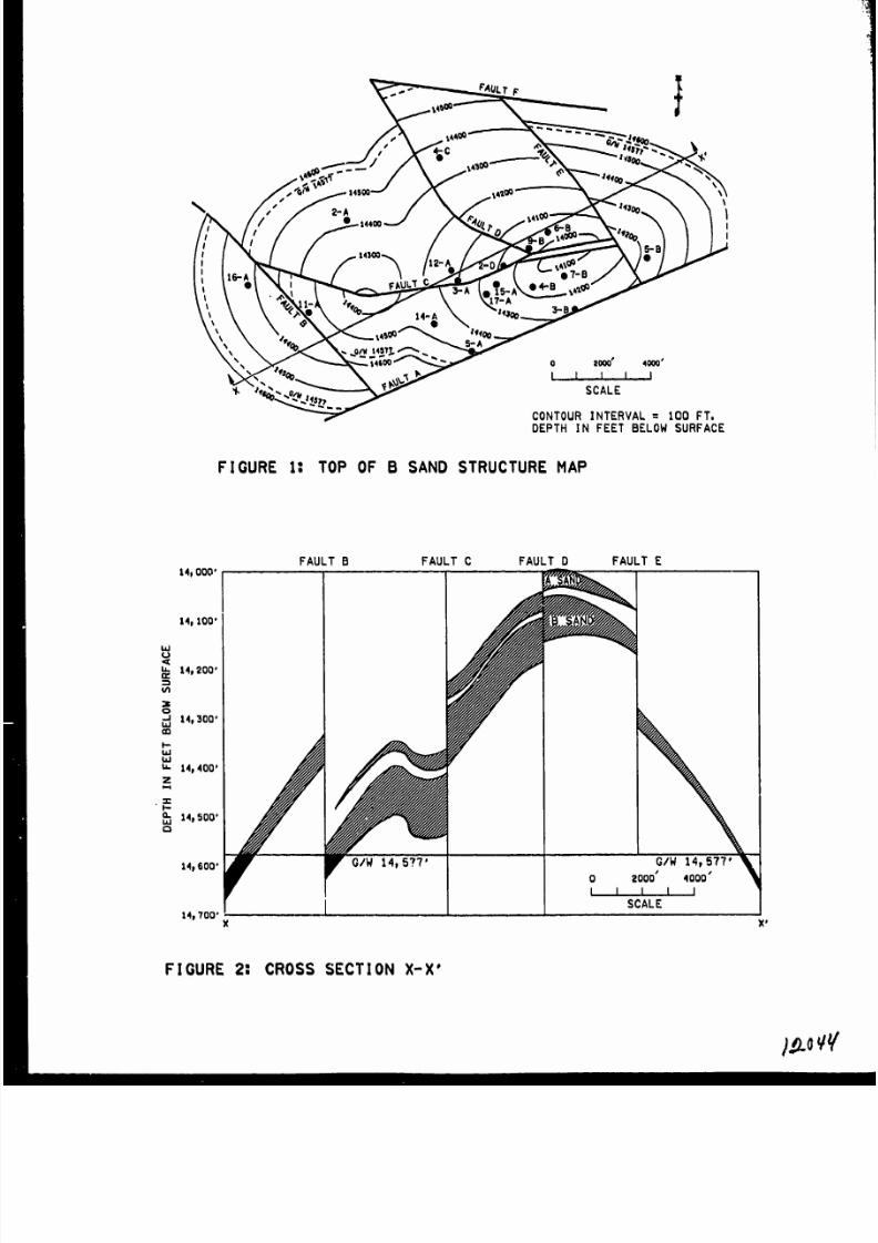
AB8TMm Figure 2 illustrates a cross-sectional view of thereaarvoir.

The purpose of this paper is not just topresent a case history, but also to provide guide- The approach to the study was first tlines for performing a reservoir study, and in analyze the avaiiable open-hole logs to obtainparticular, a material balance analysis. The average reservoir properties and to estimatestudy involved manipulating a complex material volumetrically the original gas-in-place. Thbalance equation into forms which isolated certain initial OGIP astimete was low, just slightly aboveinput parameters. The forms ware us graphically the cumulative production through August 31, 1981$not only to estimate tha OGIP, but also to verify the effective study date. Average reservoir prop-thoee parameters used in the analysis. Production erties were adjusted within the range odecline curves were used in conjunction with the reasonable uncertainty eo that this estimate wouldmaterial balance equation to predict future reser- agree with matarial balanca results.voir performance. Theoretical recovery calcula-tions justified the future predictions. Using production data to estimate the move-

ment and location of the gasfwatar contact and thaI~ODUCfIOU adjusted reservoir properties from the log analy-

sis, water influx was estimated volumetrically atThis report summarizes a reservoir study per- three different times in t h past. Several Hurst-

formsd cm an ovar-pressured, retrograde condensate Van Everdingen water influx mcdels were comparedgas field with partial water-drive. Tha purpose with volumetric influx estimates, and the modeof this etudy was to estimate the original gas-in- which comparad the best was used to model waterplace and to determine the remaining reserves, influx for material balance calculationeofirat, with the present producing wells, andsecond, with additional production from a poseible Two other material balance input parameters,recompletion. gas leakage and formation compressibility, were

also difficult to estimata and required juatifica-The gaa field ie located on-shore in t ion. The reservoir pressurz history indicated

Louisiana. Ei=i,teen wells penetrated the forma- that gas leakage from the reservoir had occurredtion of intereat, twelve wara completed in this during the first several yeara of production.reservoir ae producing wells, and six are Early gas production values required adjustment tocurrently producing. Complying with the esi r s account for the volume of gae which le6ked off.of the operating company, well names were changedand the name and exact field location have been Analyses of over-pressured reservoir tend towithheld. be complicated by larga formation compressibility

(Cf) terms, so a Cf value f or this resarvoir wThe raservoir consists of two main sands, the needed for an accurate material balance

A and B atringers, at m average depth of 14,300 analyaia.1J2~3 Corralationrs for formation com

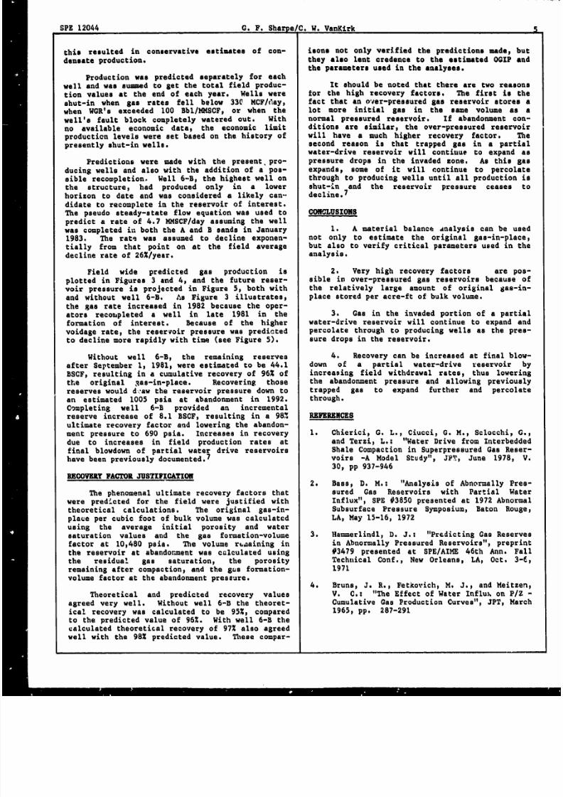
feet and an initial pressure elightly greater than preasibility, howavar, are approximetiona at best)11,800 peia (0.82 psi/ft), As is common in The value used, therefore, required some rigorousLouisiana, a salt dome deformed tha sand beds into justification.a highly faulted anticline. Table 1 awmnarizesreservoir rock and fluid properties. Figure 1 is Onca the input parameters were acquired,a structure map of the top of the B sand, and material balance model was developad to estimate

tha original gas-in-placa. Although thie modaccounted for reservoir retrograde condentsation~

References and illustration at end of paper. it should be noted that the reservoir condensatevolume was a relatively insignificant term in the

8/11/2019 (PA)-. Sharpe-. SPE 12044


2 A RESERVOIR ENGINEERINGSTUDYOF AN OVER

analy8i8. Resulte from material balance calcula-tion also verified the water influx modnl~ thevolume of gae leakage, and the formation com-pressibility term used.

Compared with the analyeie of the pest?future prediction were not eo complex. Gas pro-duction wae projected from production declinecurves. The water influx model that wae justified

in the paat analyeia was used to estimate when thewater contact would reach producing wells and topredict when fault blocks would water out. Theresulting production and water influx estimateswere input into the meterial balance equation topredict future reservoir preaeure. Using theabandonment pressure estimated from the materialbalance calculationss the predicted final aerecovery factor was justified with theoreticalcalculations,

AIIIUYSIS OF PAST PESFORXAI$CE

Field History

The first well drilled in the field appar-

ently blew-out.Absolutely no information is

available about this well including the datedrilled or ite location.

A second well, the 2-A, was drilled and com-pleted in the B stringer in July 1953, It pro-duced 3.0 billion standard cubic feet (BSCF) ofgas from August 1953 to June 19543 whan it wasshut-in to install high pressure down-hole aquip-ment. During that time period the reservoirpressure dropped from 11$800 psia to 11~450 psia.

For the next two and one half yeara there wasno production from the field until the 2-A wasbrought back on line in January 1957. Howevar,when the pressure was measured in 1957 it had?eclined to 10S480 psia. Gas les~ing from thereservoir through either wall 2-A r the firstwell (the blow-out) had apparently reduced thepressure 970 psia during the shut-in period.Further analysis indicated that the leakagecontinued another year and a half after 1957.

Because of the gas lost during the blowoutand the unknown volume of gas leakage during theehut-in period, January 1, 1957, wae used as theeffective starting dete and 10 480 psia as theinitial reservoir pressure for the study, The1957 starting date was important also because well11-A, which wae drilled in late 1957P was thefirst well whose logs showed the gas-water con-tact. Based m the data available for this study,it was impossible to estimate the gae-water con-tact location in 1953. Therefore, consistentresults were obtained by using the 11-A contac:location for volumetric calculations and aninitial time of January 1, 1957$ for the materialbalance analysis.

The field production history from January 1,1957, through August 31, 1981 (the date fror whichprediction etarted), can be seen in Figures 3 and

lRESSURED, PARTIAL WATER-DRIVE GAS FIELD SPE 12044

4. A total of 11 walls produced 597.1 BSCF of gaeduring that time period. i ve of those wells wer estill producing in September 1981$ and a sixthwell has been completad since then. Of the aixshut-in wells, one was apparently abandonedbecause of low gas production rates and the etherfive becauee of high water production rateet

The field preseure history was obtained from

fairly frequent ehut-in bottom-hole pressuretestsO Reservoir pressure is plotted versus timein Figure 5 and versus cumulative gas production(Gp) in Figure 6. Figure 6 also illustrates notonly the PIZ vereua Gp plot, but also the P/Z plotwhich accounts for rock and water expansion.Pressure data from wells in different fault blocksand from wells completed in different zonesindicated that s1l fault blocks wer e in pressurecommunication, as wer e the A and the B sands.Material balanc~ calculations? therefore wereperformed on the reservoir as a single container.

Volumetric

Open-hole wireline logs from 17 wells drilled

in the field were analyzed to determine averagereservoir properties and to estimate the originalgas-in-place. The analyais was complicated by thefact that only old electric logs were available onthe first five wells drilled. Also, a few of theother wells had incomplete log suites, whereeither resiativity or porosity logs wera notavailable.

Whenever poesible, conventional methods wareused to calculate wavar saturation. Using a 60%water saturation cut-off, the net oil thicknese(So*@*h) for each well was calculated and plottedon an “ieovol” ma P (no porosity cut off was usedbecausa log values were never balow 15%). Thiewas done separately for each sand stringer. Theisovol maps gave an OGIP estimate of 604.5 BSCF asof January 1, 1957. Since almost 600 BSCF of gaahad already been produced in late 1981, this OGIPeetimate was considered to be low. Becauaeincreasing the reservoir size could not be jus-tified, calculation were made to detarmine howmuch the average porosity and water saturationwould have to change to ge t an OGIP of 670 BSCF$the value obtained from material balance calcula-tions.

Sevsral iterations were required t o make theneceaaary porosity and saturation adjustments.The average porosity value was increased slightlyand the Humble and Archie equations were used tocalculate the resulting change in average wateraaturationg The new values wer e then used tocalculate the OOIP. This process continued untilthe volumetric agreed with the material balancacalculation. Adjusting the average poroeity from21% to 23% changed the estimated average watersaturation from 23 to 20 and the estimated OOIPto 670 BSCF. An average porosity of 23 isreasonable and well within the range of valuesinterpreted from wireline logs. The adjustedporosity and maturation vslues, therefore, wereconsidered to be correct and were reueed in allwater influx and material balance calculation.

8/11/2019 (PA)-. Sharpe-. SPE 12044


enm t . -in . ). em @ s . . l P l P w V...II.I A.Drcl A*V-V “. A’. “Uca. p=,”. “, ,=,&&\& & 3

Water Influx the last two pressure points implies thet waterinflux was act’ ally beginning to keep up with the

From the ?roduction and preaeure histories, lower r e se rvoi r withdrawal rata. Further justi-it was apparent that water influx was providing fication came from actual material balance cal-energy support to the field. Moat wells in the culatiomsg To produce con8i8tent original gaa-in-field produced relatively water free for signifi- place estimates from incremental analyses betweencant portions of their hiatoriee. At various the last thrae prea8ure points required the uae ofpoints in time, howaver, the water-gaa ratios water influx valuee larger than the original(WGR) in certain wells began to increase steadily, Hurst-Van Everdingen eetimetes.

indicating an encroaching aquifer, The concavedomward shape of the P/Z versus Gp plot (Figure From known geologic conditions about the6) alao seemed to be ~he product of a partial re8ervoir, it is likely that the aquifer iswaier-drive reeervoir. A8 the figure divided into several fault blocks and extendsillustrates, accounting for rock and water expan- beyond a radius ratio of 1.6. A faulted aquifersion etaightened the plot slightly, but it is model explaina the apparent later increase instill concave downwarda. The reason the plots aquifer 8upport, Although the aquifer extensionbend downward8 ie because early in the field life contributed pres8ure support from the beginning$the gaa compressibility i8 small (due to the high becauae of the restricted permeability acroaapressure) and the aquifer expanaion contribute fault8, the dimen8ionle8s time and the relatedproportionally more pressure support than later in dimen8ionle8a water influx (8ee Hurst Van-the field life.4 Extrapolation of the earlY Everdingen method5) increased at a very slow rate.portion of the P/Z plot, therefore would have However, by 1977 the dimensionless water influxindicated a very large OGIP value. had become large enough, the cumulative preaaure

drop had become large enough, and the water influxModeling water influx was difficult with no rate from the Hur8t-Van Everdingen modeled aquifer

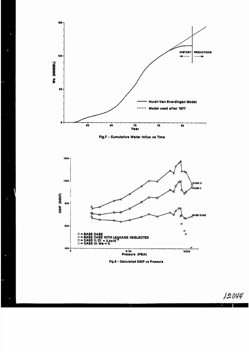
knowledge of the aquifer 8ize. The approach used had become small enough that the aquifer beyondwaa to estimate water influx volumetrically and the radius ratio of 1.6 began to contribute acompare these calculation with Hurst-Van significant portion of the total water influx,Everdingen models which u8ed different aquifer-to-gas radiua ratioa. Once the aquifer size was The original Hurst-Van Everdingen waterdetermined, that Hurst-Van Everdingen model wa8 influx model did a good job accounting for wateru8ed to estimate water influx fOr material balance influx through 1977, and after that point it pre-calculation. dieted influx rate8 le8s than what were needed.

Therefore, it waa assumed that the water influxThe time at which the &as-ater contact rate 8tayed constant at the 1977 rate of 4.61 MM

reached certain wells waa estimated from produc- Bbllyr. A8 Figure 7 illustrates, this model waation data. The initial gaa-water contact loca- used to estimate water influx from 1977 to 1981tion, water 8aturation, and porosity were obtained and &180 for future prediction bayond 1981.from the log analyses. The logs from two wellsdrilled later in the field life into invaded It 8hould be noted that neither the originalportions of the reservoir were used to estimate Hurst-Van Everdingen model nor the aquifer exten-

the residual gas saturation. Having obtained .sion model are necessarily corrsct. The actualthese values, the area invaded into any certain geometry, continuity, and physical propertie8 offault block waa mea8ured and the cumulative water the aquifer are unknown. The models are merelyinflux into that block waa calculated. Cum&lative mathematical emulations which reasonably accountwater influx values were summed for the total for the water influx that haa entered the re8er-field at three different points in time; mid-1906, vcir in the past. Although these models obviously id-1977, and mid-1981. are not perfect, water influx valuea obtained from

them were used t o get reasonable and consistentResults from a Hurst-Van Everdingen model material balance results, aa will be discussed

with an aquifer to gas radius ratio of 1.6 com- later.pared most favorably with the volumetricestimatea. Water influx predicted from this model Material Balance Analysisi8 plotted versus time in Figure 7.

Iiiis material balance equation u8ed in theThe two influx analyses compared fairly well analysis appears in Appendix A. It is a fairly

through 1977, differing by less than 6%. From complex expansion-equals-voidage equation which~

1977 through 1981, however, the Hurst-Van among other things, accounts for rock and waterEverdingen model estimated significantly less expansion, reservoir retrograde condensation, andwater influx than did the volumetric model. Since water influx. The equation ia broken down intothe volumetric numbers are probably closer to its major component8 in the appendix.being correct, it was apparent that the aquiferbeing modeled by the Huret-Van Everdingen method Most of the input parameters were known fromwas beginning to see additional outside support. the production and pre8sure hietories and from anThie theory is supported by the PIZ versus Gp plot analysis of a reeervoir fluid sample taken early(Figure 6). Until the lact few pressure points, in the field’s life. The water influx model hasthe P)Z curve is concave downward, indicating that already been discu8sed. The most significant.throughout that time period the water influx rate unknown parameter was the formation compress-was insufficient to replenish voidage and maintain ibility. Newman’s correlations were used toreservoir pressure. However, the leveling off of estimate that value,6 If the formation were con-

8/11/2019 (PA)-. Sharpe-. SPE 12044


4 A RESERVOIR ENGINEERING STlll)Y (M’ AN (WI?R-PR17S WRET. UARTTAT. UATPR-I)RTVU I AC ?rrmrn SPE 12044- -—-------- . --------------- ----- -. .. . . . . .. . ---------- . . .. ...-..” “..-”..–”..* ..4 “m” .-*-M” “

solidated, the estimated compressibility would be2.4 x 10-6 vol/vol/p8i.

place, but they aleo verified some of the criticalIf the formstion were parameters used in the analyeiae Three cases are

unconeolidated~ a value of 14. x IO-6 vol/vol/pei plotted in Figure 8; the firet was the base cane,would be eetimated from the correlations. The the eecond used the lower formation com~ree8-latter value was used because Gulf Coast sande ibility term, and the third neglected watertend to be unconsolidated, especially when over-preeeured.1$2~3

influx. The consistent baee case OGIP values lendSince the formation compreee-

ibility turned out to be a significant drivingcredence to both the water influx model and forma-tion compressibility term.

energy ~ that value was juetified later in the

material balance analysia. Two cases are plotted in Figure 9; the firstThe first step in the analysia was to manip- wae the baee case and the second waa where leakage

ulate the material balance equation into the form was neglected. The plot indicates that leakageof a etraight line (Y = mx + b) where the slope waa indeed occurring and also that it was reaaon-was equal to the OGIP and the intercept was equal ably accounted for, In addition, the intercept ofto zero. This manipulation appeare in Part 1 of the plot wae used to calculate a formation com-Appendix B. Values for “X” and “y” were cal- preseibility of 14.5 X 1o-6 psi-l, which justifiedculated at each of 21 known pressure points. An the term obtained from Newman’sOGIP value,,~~s eetimated at each point by dividing

correlations.This calculation is performed in Part S of Appen-

“X’t into Y . Eatimeted OGIP values are plotted dix C.‘ara:le preaaure in Figure Parte 3, 4, and 5 of

Append:.x C chow a sample calculation ueing this The original gaa-in-place was calculated fromanalyeieo the slope of Figure 9 to be 673 BSC)?. This com-

Low OGIP estimatee f or the first few pointspared very well with the value of 669 BSCF cal-culated from the incremental material balance

implied that not enough gae production was being analyses. Because of the large number of OGIPaccounted for from early reservoir preaaur? drope. valuee calculated from the incremental analyses~These low estimatee indicated that gas was still the result f rom that method wae weighted more thanleaking from the resarvoir. Since leakage had the Figure 9 result, and 670 BSCF wae used as theoccurred during the ehut-in period, and it was not best eetimate for the original gas-in-place ongoing to stop juet because production began againj January 1, 1957.this result was expected, Leakage was accountedfor by calculating how much production would have FUTUREPRBDICTIOIWto be increased at the early preeeure points toproduce reasonable OOIP estimetee. F:om these Future reservoir performance waa predictedcalculations it was estimated that 4.4 BSCF of using produ,,tion decline curves in conjunctiongaa leaked from the reservoir during the first with the water influx end aterial balance models.year ‘and one half of production after 1957. At The water influx model waa used to estimate whenthat time$ the pressure at the leakage point the water contact would reach the wells and tobecame low enough that gas flow from the reservoir predict when fault blocke would water out. Withceased. the OGIP estimate, the material balance model used

the estimated water influx in addition to pro-After accounting for leakage~ 210 more data jetted productionpointe were generated by doing an incremental

to back calculate the futurereservoir preseure.

material balance analysie between each of the 21preseure points. Part 2 of Appendix B illustrates In almost all casee, the gae productionthis analysis technique. Each incremental analy- decline rate for each well could be approximatedsia wae used to estimate an OGIF value, The closely by an exponential equation. When wateraverage of all these values, 669 BSCF, was used as broke through in various wells, production couldan initial beet estimate of the original gas-instill be modeled with an exponential equation butplace. A sample calculation for thie analysis at a steeper decline rate. The decline ratas inappears in Part 6 of Appendix C. the field increased an average of 68% after water

breakthrough. Future gaa production was predictedManipulation of the aterial balance equation for each producing well, therefore, using its

into another straight line form waa used not only actual decline rate and asauming that that rateto support the OGIP estimate, but aleo to justify would increaae 6S% after water breakthrough.the formation compressibility term used. This

manipulation is illustrated in part 3 of Appendix Water production was predicted after break-B. As can be seen, the slope of the line ie still through from plots of log of water gas ratio (WGR)the OGIP, but now the rock and water compress- vereue Gp. WGRvaluee in wells which were not yeibility terms have been isolated in the intercept.Valuea of “X” and

producing much water were aeeumed to increase atNyU were calculated at each the field average rate after breakthrough,

preeaure point and a least squares analysis wasused t o find the slope and intercept of a best fit The latest condensate-gae ratio for each well1ine. The resulte are plotted in Figure 9. A waa held constant and used to predict future con-sample calculation of 11x and yll values iS il~u8- densate production. At the time predictionstrated in Part 7 of Appendix C. began, the average condensate-gae ratio wa

approximately 5 STB/MMSCF. Since the reservoirThe material balance analysis results not pressure was approaching the point where the

only were used to estimate the original gas-in- retrograde condensate was beginning to rcvaporize$

—

8/11/2019 (PA)-. Sharpe-. SPE 12044


8/11/2019 (PA)-. Sharpe-. SPE 12044


6 A RESERVOIR ENGINEERING STUDY OF AN OVER-PRESSURSD. PARTIA1, WATER-DRIVE GAS FIELD sDli 19(ML.-. —-—---- .. —-----.——.- . . _--—_ ,--- -.-—-- -------- ---- .- ---- ----- “ - .-”-7

5s Van Everdingen, A. F., and Hurst W.: t~e 3. Equation of straight line where the slope equaApplication of the Laplace Transformation to the OGIP and the intercept equals the rock andFlow Problems in Reservoira~” Trans. AIME water compressibility term(194), PP. 186)305 Y =~Gp + 5.615*Cp*Boe*rac MWsc)*Bg

6. Newman? Gt H.:+ 5.615wp*Bw - 5.615Wi~/(Pi - P)Ipore yolume compzeeaibility

of Consolidated, Friable, and Unconsolidated Res ft3/psi

Reservoir Rocke Under Hydrostatic Loading”)JPT, Feb. 1973, V. 25, pp. 129-134,

X = ~Bg - Bgi) + 5.615*VC*(1 -Bg*380@rc/~rr)’/(pi - p)

7* Brinkman, F. D.: Res ft3/SCF-pei~l~ncreased Gas RecoverYfrom a Moderate Water Drive Reservoir”?preprint 9437 presented at SPE/AIME 55th

m“GSCF

Ann. Fall Technical Conf.~ Dallas) TX Sept. b = (Wgi/1-t3Wi)*(cW*9W + cf)21-24, 1980

Ree ft3/psi

APPENDIX Cs Sample Material Balance CalculationAPPERDSX A: Material Balance Equation

Calculation done at preeaure point 5, March 1960

Expanaion E Voidage 1. Constant input data:

G*[( Bg - Bgi) + 5.615*VC*(1 - Bg*380*(%c/MWrc) Pi = 10,480 psia+(Bgi/1-Swi)*(~*~ + Cf)*(Pi-P)]+ 5.615*We Bgi = 0.002746 RCF/SCF

=(Gp+5.615*Cp*Bos*380*(%c/~sc)*Bg+5.615*Wp*Bw BOS = 1.0807 Bbl/STBSwi = 20.5%

where: Cw = 3.45 X 10-6 vol/vol/psi= 14 X 10-6 vol/vol/psi

G*(Bg- Bgi) UIgas expansiongc

= 49.5 lft3G * 5.615 * Vc = reeervoir volume Of

retrograde condensate~sc = 157$7 / -mole@C = 48,3 ;ft3

G*5,615*vc*Bg*380@rc/~rc = equivalent gasvolume of retrograde condensate

MWrc = 178,3 / -mole

G * (Bgi/1-Swi) * (OW * Sw + Cf) * (Pi - P) = 2. Input data at pressure point:rock and water expansion

5.615 * We = water influx P = 9804 psia

Gp * Bg = gae production Bg = 0,002821 RCF/SCF

(50615*Cp*B08*380*&C/MW8C)*Bg = equivalent Vc = 0.37 Bbl/MMscf

gas volume of produced condenadte Gp u 3S004 + 4.4 = 42.44 BSCF

5.615 *Wp * Bw =water production Cp = 696.98 MSTBWp = 94.65 MBbl

with all volumes in reservoir cubic feet, Bw = 1.036 Bbl/BblWe = 8,3 MMsbl

APPIWDIX B: Munipulationa of the HE Equation 3. Ctilculate expansion factor, Xj:Gas = 0.002821 -

1. Equation of straight liue where slope equals0.002746 = 75.0*10-6

CondensateOGIP and intercept equals zero:

= 5.615*0.37*10-6*(l-0.002821*380*48.3/178.3) = 1.47*10-6

Y = (GP + 5.615*Cp*Bos*380*f?sc/MWsc)*BRock and Water =(0.002746/l-O.205)*(3.45*0. 2

+ 5.615*Wp*Bw - 5.615*We Res ft 5+ 14)*(10480-9804)*10-6 = 34.3*1o-6

Total = 11o.77*1o-6 Res ft3/SCFX=(Bg- Bgi) + 5.615*VC*(1- Bg*380@rc/MWrc)

4+ (Bgi l-Swi)*(Cw*Sw + Cf)*(Pi - P) 4. Calculate total voidage? Yj:Ree ft /SCF Yj (42.44*109 + 5.615*696.98*103*I .O8O7*38O

*4g,5/157,7)*0,00282~+50615*94.65*103*1,036m.G SCF - 5.615*8.3*106 = 0.075095 MMMRes ft3

b-o 5. Estimate OGIP at pressure point:

2, Ucina lIXU and IIyll values from part l) do incr@- OGIP = 0.075095/110.77*10-6 = 678 BSCFmental analysis between each pressure poiut 6. Estimate OGIP from incremental analysis between

y=mX+b=G*X+Opreseure points 4 and 5S

Y3=G X3 X4 - 88t9~~10-6 Rea ft3/SCFy5mG*X5 Y4 - 0.059775 MHMRes ft3(Y5 -Y3) =G* (X5 -X3] (X5-X4) = 110(77-88,91G = (Y5 - Y3) / (x5 -x3) = 21.86*10-6 Rea ft3/SCF

(Y5 -Y4) = 0.075095-0,059775Where X5 and X3 and Y5 bnd Y3 are “X” and “Y” - 0,015320 MM Res ft3values calculated at pressure points 5 and 3. OGIP = 0.015320/21.86*10-6 = 701 BSCF

8/11/2019 (PA)-. Sharpe-. SPE 12044


GIru AGWVT W, A’, GJ119h~S/U, W, 1a11hAL6

7. Calculate “X” and “Y” values for straight line TABLE I

equation where the elope equais the OGIP and theintercept contains the rock and water compresei- SESERVOIR ~ ~ PLUIDPROPERTIESbility term,

x ~0.002821-O.002746) - 5.615*0.37*10-6*(1 - 0.002821*38?*48.3/178.3fl / (10,480- Average Depth 14,300 feet subsurface9804) = 1.131*10-i Res ft3/SCF-psi

Productive Area:Y = ~42.44*109 +5,615*696.98*103*1,0807

*49,5/157,7)*t),00282] + s.61s*94.65*103 A zone 1,700 acr*1.036 - 5,615*8.3*10~/(1048G - 9804)

= 109.0*103 Res ft3/pei B zone 3,850 ac

8. Calculate formation compressibility from Average Grooe Thickness:intercept of Figure 9,

A zone 22m = 6?3 BSCFb = 35.39*103 Res ft3/psi B zone 62

Cf = 35.39*103/(673*109*0.002746/l-O.205) -3,45*1O -6*0,205 = 14.52*10-~ vol/vol/psi Average Net Pay:

NOHENCIATURS A zone 20

Bg = gas formation-volume factor, FVF, at pressure B zone 52 fP, Rea cu ft/SCF

Bgi = gas FVF ac initial reservoir pressure? PorosityRes cu ft/SCFBoa = stock tank to separator oil-volume factor, Initial Water Saturation

bbl/STBBw = water FVF at pressure P, Bbl/Bbl Residual Gas SaturationCf = formation compressibility, vol/vol/paiCp = cumulative condensate production~ STB Initial Pressure (1952) 11,800 paCw = water compressibility, vollvol(paiG = original gae-in..place, SCF Initial Study Preeeure (1957) 10,480 pGp = cumulative gae production, SCFMWrc = reservoir condensate molecular weight, Reservoir Temperature 250

lbs/lb-rnoleMWSC= separator condensate molecular weight, Permeability 100

lbs/lb-moleP = reservoir preetiure at any time psia Formation Compressibility 14 x 1o-6 vol/vol/PsiPi = initial reservoir pressures psia

Swi = initial water saturation fraction Gas Gravity (air = 1.0) 0Vc = ratio of reservoir condensate volume to

OGIP, bbl/SCF Condensate Gravity 480We = cumulative water influx, bblWp = cumulative water production bbl Water Salinity 130,000~rc = reservoir condensate density, lba/cu ft~ec = separator condensate density, Ibslcu ft Water Compreeeibility 3,45 x 10-6 vol/vol/p8i5.615= CU ft/bbl380 = SCF/lb-mole

8/11/2019 (PA)-. Sharpe-. SPE 12044


““w1 1 1 I 1

SCALE

CONTOUR INTERVAL =100

FT.DEPTH IN FEET BELOW SURFACE

FIGURE 1: TOP OF B SAND STRUCTURE MAP

FAULT B FAULT C FAULT D FAULT E14,000’ I

I

14, 1 ’

LL lg

14)200’

5g

~ 14,300’m1-Ww~ 14,400’z

F~ 14,500’Q

14,600’

i4, 700 ’x

r

‘G/W 14~5?7’, .

TGIW 14,577’

0 2000’ 4000‘7 ~ I I JI I I

SCALE

F I GURE 2: CROSS SECTION X-X’

8/11/2019 (PA)-. Sharpe-. SPE 12044


8/11/2019 (PA)-. Sharpe-. SPE 12044


aooo

I 1 I I 1 1 1 1 (

90 0s 70 80 86 soYuar

Flg.6 - Reoorvolr Pressure v. Time

10QOO

aooo

6000

4000

2000

0

\

PREOWIRE

\

PIZSOON8TAN

(). ~REeSIJRE

:: ;j: ql-((ow”sw+cf)/( 1-swl))*(Pl-P)

1 1 I I 1 I100 aoo 000 400 600 000 700

Clp (Bf3CF)

FIQ,6 - P/Z v. Gumulat lve Qaa Produ ot lon

8/11/2019 (PA)-. Sharpe-. SPE 12044


1s0,.”’

,. ’”

Pn6DloTloN8

/— Hurst-Van Everdlngen Model

‘----- Model used efter 1077

0 /1 1 1

001 1

cm 701

76 10

Year

Flg,7 - Cumulet lve Water Influx ve Tlmo

...-

’l

x

o ~~ E CASE

x = BASE CASE WITH l.E~KAQE NEQLECTED = CASE 11:Cf - 2,4xIO-A = CA E Ill: w. m o

400 + IKoo

110000

Proowo (P81A)

Fl g,6 - Oaloulat od OQIP vs Proawa

8/11/2019 (PA)-. Sharpe-. SPE 12044


()= BASE CASE~ = CASE [[: LEAKAQE NEQLECTED

CD

‘X’ (I?ES FTg ;:CF-PSI X 107)

Flg,8 - Stral ht Line Plot where the Slope= OQIP\nd t e Interoept equals the Compreaalblllty Term

(pa)-. sharpe-. spe 12044

Documents