Staff Papers Series

P86-49 December 1986

Assessing Food Production Potentials in the

Final State of Stationary Populations

by

Adolf Weber

L5

Department of Agricultural and Applied Economics

University of MinnesotaInstitute of Agriculture, Forestry and Home Economics

St. Paul, Minnesota 55108

How much land does a man need?Leo Tolstoy 1886

Assessinq Food Production Potentials in the

Final State of Stationary Populations*

by

Adolf Weber

*I am indebted to Norbert Gebauer, Institut fur Agrarpolitik

und Marktlehre, University of Kiel, who has conducted the

planimetric work and the calculations.

Staff Papers are published without formal review within the

Department of Agricultural and Applied Economics.

The University of Minnesota is committed to the policy that

all persons shall have equal access to its programs, facilities,

and employment without regard to race, religion, color, sex,

national origin, handicap, age, or veteran status.

2

1. Introduction and Overview

2. Assessments of Global Production Potentials

2.1 Approaches in the Natural Sciences

2.2 Approach of Agronomists

2.3 Global Comparisons and Assessments

2.4 Approaches Developed by FAO/IIASA

3. Food Production Potentials or the Theoretical Maximum of

Food Production

3.1 Theoretical Yield Potentials in Countries

3.2 Present Grain Yields Versus Potential Yields

3.3 Food Production Potential in the State of a Stationary

World Population

3.4 Food Comsumption Levels in Countries at Stationary

Population

4. Conclusion

Endnotes

References

Appendix

3

1. Introduction and Overview

Since Malthus many authors have elaborated the nagging

question "How many people can be provided with food on earth?".

Thus, the purpose of this study is to explore and examine

concepts which try to measure the food production potential of

the earth.'

Two groups of approaches characterize the literature. The

first group derives its conclusions from comparing differing

yield levels between countries, areas or agricultural experiment

stations. One argues quite reasonably that through the

application of modern technologies, low productivity land can be

developed to higher yield levels. However, the theoretical

maximum of food production is not specifically assessed. This

may lead to an underestimation of the earth's food production

potential only because observed yield levels are the basis of the

assesments made. Pertinent to this approach is that as soon as

the extent of the cultivable land, yield, and comsumption levels

are determined, the number of people to be nourished on earth can

be calculated. Because this approach has an insufficient

coverage in space and in time, it will not be considered further.

The second group of approaches is more recent and scholarly

conceived. Botanists and agronomists have assessed

quantitatively the actual and theoretical performances of the

world's various natural vegetation and agricultural production

systems. In Section 2 an attempt will be made in presenting the

basic concepts with global assessments.

4

However, the natural scientists' approach is mostly applied

to various aggregates of global, continental or agroclimatic

zones which disregard national boundaries. This study is

designed to transform and adjust global, continental and

agroclimatic zones' estimations of the food production potential

to country levels. The food production potential of countries is

then related to estimations of its stationary population.

Various utilization rates of the food production potential are

assumed. This permits exploration of the possible food

consumption levels in the final state of a country's stationary

population.

This study has to rely on many assumptions and

generalizations. Some calculations and estimations lack the

desirable accuracy. Further, the time horizon appears, compared

to current problems of the world food economy, rather distant.

But it is hoped that a better understanding of how to evaluate

the food production potential of the earth, in the world's

regions and countries is the consequence.

2. Assessments of Global Production Potentials

2.1 Approaches in the Natural Sciences

A first attempt of assessing nature's production potential

has already been made in 1862 by Liebig when he estimated the

size of the primary production of plants on the earth. The next

step in quantifying the earth's primary production was taken by

botanists. Lieth (4, 5, 6) developed (1972) for the world a

complex model of estimating primary productivity (biomass) for

5

the main types of vegetation (forests, savannahs, grassland,

cultivated land, etc.). To model nature's production function at

various latitudes and locations, an inventory of the world's

climate represented the first step. Lieth used data on

temperature, precipitation, evaporation of 1,000 metereological

stations from all over the world. The results were presented and

mapped in terms of dry matter production for the land and the

sea. He estimated the earth's annual total dry matter production

at 155 X 109 tons, of these 55 X 109 are produced in the sea and

100 X 109 tons on the land.

To get his share of the biomass, man is and has permanently

been in competition with other living organisms. Further, only

the smaller part of the annual biomass produced is accessible to

man and edible. Therefore, man has to use his domesticated

animals which convert for him some of the inaccessible fibrous

material into edible food. Under several assumptions Lieth

estimated the number of people which could be supported by the

earth's ecological system at 7 to 15 billion people.

The approach of botanists has its virtues. It emphasizes

that primary productivity or biomass production occurs

independently of man, but differs in amount according to natural

resources available at each location. However, the estimation of

the world's total annual biomass production out of broadly

defined vegetation systems remains, for the purpose intended,

crude and too summary. One can rarely derive the proper share of

food out of total biomass production which could be made

6

available to man.

2.2 Approach of Agronomists

An estimation of the earth's food producing potential was

undertaken in 1975 by Dutch agronomists of the University of

Wageningen in the Netherlands (1). It was part of a project (11)

"Food for a Doubling World Population" which was initiated in

response to the Club of Rome's world-wide known study "The Limits

to Growth."2

The theoretical framework of the assessment procedure was

developed by the Dutch agronomist De Wit (12). He considered the

photosynthetic potential of cultivated plants as a function of

location, latitude and an inventory of the world's climate (solar

energy, monthly air temperature, precipitation, evatransporation,

leaf canopy, etc.). The results were summarized in a table for a

standard crop 3 (conceived as a C3 plant). The authors Buringh,

van Heemst and Staring (1, p. 27) described the procedure as

follows: "indicating for the middle of every month of the year

the daily totals of photosynthesis on every clear (PC) and

overcast (PO) day of various latitudes. PC and PO can be derived

from this table for any location by linear interpolation. These

totals, calculated on the basis of the light climate, can only be

reached when the average temperature is reasonable. This is

presumed to be the case when the average temperature is 10°C or

higher."

They used the following apparatus of formula to estimate the

mean monthly gross photosynthesis (CAR):

7

(1) CAR = ID (F - PO + (1 - F) . PC)1 where

CAR = Gross Photosynthesis expressed in- kg carbohydrate

per month and hectare,

ID = the number of days in the month;

F = the fraction of the time when the sky is overcast

and

(2) F = 1 - - H- 1 where

h = mean monthly sum of hours of sunshine, local data;

H = the monthly sum of maximum hours of sunshine.

Carbohydrates are transformed into Dry Matter (DM) by

multiplying with the factor 0.65 which yields:

(3) DM = 0.65 X ID (F - PO + (1 - F) - PC).

The formula can only be applied, however, when the average

temperature is for more than three months higher than 10°C and is

written as:

(4) DMY = DM X MO where

DMY = Dry Matter production per Year and

MO = Number of Months above 10°C subject to M053.

The so calculated potential dry matter production contains

still the roots, stems, leaves, flowers, and fruits. Under the

assumption that the dry matter production is composed as follows:

Roots and stubble (25% of DM), straw (37.5% of DM), grain (37.5%

'This formula was later changed into:(la) CAR = ID (F= - PO + (1 - F= ) - PC) to permit a non-linearinterpolation between the two states of the sky (clear orovercast). The formula now takes into account all diffuseradiation and may lead at some locations to higher estimations offood production potentials (9). In this contribution only theoriginal calculations based on formula (1) have been considered.

of DM) with 2% as harvest loss and a moisture content of the

grain of 15% the maximum production in grain equivalents is then

calculated:

(5) MPGE = DMY x (0.75 X 0.5 X 0.98 / 85) X 100

or MPGE = 0.432 X DMY.

However, the conditions of growing crops are rarely optimal

in the world's agricultural regions. Nutrients are missing or

the water supply is the limiting factor. A proper soil inventory

had to be developed. From the world's soil (and water)

inventory, the authors introduced reduction factors for poor

soils and for water deficiencies. The basis for applying

reduction factors (ranging from 0 to 1) have been maps of 222

broad soil regions of FAO/UNESCO which had a scale of

1:15,000,000. The areas, with respective water deficiencies,

were derived from related studies on water availabilities. The

lowest of both limiting factors were then applied to reduce the

tabulated photosynthetic performance in each of the 222 soil

regions.

Pertinent to this approach of estimating the MPGE is the

appraisal of the potential agricultural land and an assessment of

the potentially irrigable arable land (1, p. 50). The MOIRA

elaboration includes further assessments of development cost

categories, the distribution of land productivity classes and the

topography of soils (lowland, upland, deserts, mountains) in the

world's regions. More details can be derived from the source.

The final calculation of the MPGE for the world in total can be

9

found in Table 1.

2.3 Global Assessments and Comparisons

Nature has had millions of years time to maximize biomass

production on earth. Thus, nature maximizes at each location and

climate the sun light's energy by a diversity of plants. The

more optimal the growth conditions, the higher is the biomass

production and the diversity of contributing plants. This is

revealed in the rich variety of plants growing in lushy tropical

forests and the very small number of plants and tiny biomass

production in the world's deserts and tundras.

However, production targets of nature are not identical with

those of man. Man has, compared to nature, at his disposal only

a reduced number of cultivated plants which guarantee his

survival, because he can not live from tree branches, leafs,

ferns, moss, etc. Therefore, man has been forced to increase

food production by enlarging his share of cultivated plants in

total biomass production.

By converting nature's annual biomass production and the

food production (actual and potential) into energy units (Joule

CJ3), one can compare the respective dimensions of the botanists'

and agronomists' approaches (Table 2). In 1964-66 world food

production represented only 3.2% of total biomass production.

The above assessed food production potential would finally

represent 38% of total biomass production on land (12).

2.4 Approaches Developed by FAO/IIASA

The methodology developed by the Wageningen group has been

-10-

Table 1: The Absolute Maximum Production of Grain Equivalents (MPGE)World, Continents

Arable Potential MPGElanda agricultural tons/1982 cropland hectare/ MPGE MPGE

Region Million Hectares year 109 t in %

South America 139 617 18.0 11.1 22.3

Australia 47 226 10.4 2.3 4.7

Africa 183 762 14.3 10.8 21.8

Asia 506 1,081 13.2 14.3 28.6

North andCentral America 273 629 11.3 7.1 14.2

Europe 322 399 10.5 4.2 8.4

World 1,473 3,748 13.4 49.8 100.0

aIncludes permanent crops. The arable land of the U.S.S.R. has beendivided into 182 million hectares for Europe and 50 million to Asia.

Source: MOIRA, p. 25-49. -FAO, Production Yearbook 1983.

-11-

Table 2: Estimated Annual Biomass Production on Earth compared with the

World Food Production in 19 6 4-66c and the World's Absolute Maximum

Production in Grain Equivalents (MPGE)c in Joule (J)d

lj~~ NPHOTO-INPUT SYNTHESIS YIELD

100% 1.8 '1021J TOTAL BIOMASS

Biomass not used as food (Land)

by man (trees, shrubs,--- SUN ferns, moss, leafs, stems,

> SUN __roots, stubbles, flowers,plants in freshwater, etc.)

WATER

38% - - - - - - - - - -0.7 1021 J or MPGE|LABOR ) Theoretical food production

potential

NUTRIENTS

CAPITAL Sphere of expansion

213.2% World food production 1964-66 0 022 10 J

aAccording to Lieth (1972). Without biomass produced in oceans. CMOIRA.

dDry matter production and grain equivalents have been converted into energy

units (1 Joule = 0.2388 cal) under-adopting the following conversion ratios:

one g of dry matter = 4.23 kcal and one g of grain equivalent = 3.3 kcal.

12

further pursued by a group of researchers of FAO/IIASA (3, 8).

They differ in details of the climatic and soil inventory, e.g.

they use for assessing the food producing potential a soil map of

larger scale (1:5,000,000 instead of 1:15,000,000). Instead of

estimating the production potential in 222 broad soil zones, they

consider agroecological cells of 10,000 hectares in each of the

117 developing countries (without China). Instead of a standard

crop, they assess the performance of several suitable food crops.

Finally, the FAO/IIASA research group distinguishes different

levels of inputs (low, medium or high). The intention is to

determine those countries which don't even have at the high input

level enough food in the year 2000. However, conclusions for the

long run are difficult to draw because the high input level is

neither quantitatively defined nor is the underlying production

function explained.

The FAO/IIASA approach is not followed here despite finer

details in soil and climate inventory and the broader range of

food crops considered. The FAO/IIASA approach has the

disadvantage that it covers only one part of the world. Further,

it can not be derived from the study how the various crops were

aggregated and which proportion of the food production potential

in each agroecological cell should be mobilized by the year 2000

to meet the food requirements.

Similar studies seem to have been undertaken for the

U.S.S.R. by Soviet scientists (2, 7). However, the methodology,

data and results have, until now, not been accessible to the

13

general public. This is mentioned here only as an indication of

how appealing the methods of estimating food production

potentials have been.

3. Food Production Potentials or the Theoretical Maximum of Food

Production

3.1 Theoretical Yield Potentials in Countries

As mentioned above, the estimation of food production

potentials in the MOIRA-Study started from 222 soil zones. The

aggregation of grain equivalents was conducted as continental and

world totals (Table 1). The disaggregation to country levels is

planimetrically done in the following Figures 1 to 6. The

appendix contains the elaborated country data in three tables.

The published maps of soil zones in the MOIRA-study had to

be disaggregated and allocated to very uneven sized countries.

The allocation is easy if a country belongs only to one soil

zone. Some countries have extremely rugged national boundaries

which hampers planimetric accuracy. Most of the larger countries

belong to several soil zones (like Brazil, China, the U.S.A., and

U.S.S.R.). Brazil has 16 soil zones, China 13, the U.S.A. has

17, but the U.S.S.R. has 30 different soil zones. To give only

one example of the diversity of production conditions in large

countries: the highest yield class in the U.S.A. has 22.6 tons

of GE per hectare, however, the lowest reaches only a theoretical

yield of 5.2 tons. Therefore, in most countries a complex

weighting of the various soil zones had to be pursued. To

minimize possible differences between MOIRA's continental and the

14

planimetrically derived country results, some, but minor

balancing calculations, were applied. Additionally, tiny

islands, many small states, the small Levantine countries

(Israel, Jordan, Lebanon), countries on the Arabic peninsula

(Yemen [North and South], Oman), both Koreas and Switzerland have

been excluded. Presently, these countries do not cover more than

1% of the world grain (or food) production.

The MOIRA-Study distinguishes six land productivity classes

(Table 3). Forty-five percent of the world's potential

agricultural land has theoretical yields of more than 15 tons of

grain equivalents. It is concentrated in areas where neither

frost nor extended droughts interrupt the year's vegetation

period, typical for the lower latitudes in Latin America, Asia

and large parts of Africa. The special distribution of six land

productivity classes among all continents is revealed in Figure

1. There are a few countries which have a potential of less than

five tons GE per hectare (Mongolia, Mali, and Niger) or more than

25 tons GE/hectare (Egypt and Bangladesh). The countries of

Europe, Turkey, China, Japan, Argentina and the United States

have on the average a theoretical yield potential of up to 15

tons GE per hectare of their partly large territories. Northern

countries, Chile and Australia reach only 10 tons GE per hectare

whereas many tropical countries can reach more than 15 and 20

tons GE per hectare.

Moreover, it has to be mentioned that the estimations of the

food producing potential are based on potential agricultural land

-15-

Table 3: Distribution of Soil Productivity Classes in Million

Hectares, Maximum Production in Grain Equivalents (GE)

Region Productivity Class (GE/tons/hectare)in Million Hectares

I II III IV V VI<5 >5-10 >10-15 >15-20 >20-25 >25

South America 12 -- 108 287 185 3

Australia, New 60 68 26 19 49 --

Zealand

Africa 93 92 95 335 135 5

Asia 197 51 352 214 135 69

North & Central -- 342 87 144 48 --

America

Europe 1 151 224 12 4 --

Total 3,602 362 704 892 1,011 556 77

in % 10 20 25 28 15 2

Source: MOIRA, p. 39.

r-4 nd

0~~~~~~~~~~~~~~~~~~~14)

H~~~~~~~~~~~~~~~~~~~ -I~~~~~.

-4

O~~~~~~~~44 1B

:4~~~~~~~~~~~~~~~~~~~~~~~~~~~~~~~~~~~~~~~~~~4b

4 -~~~~~~~~~~~~~~~~~~~~~~~~~~~~~~4C

0 ~~~~~~~~~~~~~~~~~~~~~~~~~~~~~~~4A 5 145

O.t 014.5

co

>~~~~~~~~~~~~~~~~~~

4-) tO

o I ,

:1 4.4 ~ ~ ~ ~ ~ ~ ~ ~ ~ ~ ~ ~ ~ ~ ~ ~~ 00~.

10

0 11

C, C)

at

co

0k-

co

rid

'I'···

17

-- not on actually cultivated land which is only 40% of the

total potential. Thus, one can reasonably assume that the actual

crop land use already covers in each country the more fertile

soils.

This permits the conclusion that the theoretical yield potential

on the actual crop land must be much higher than on the potential

crop land.

3.2 Present Grain Yields Versus Potential Yields

More than half of the energy directly consumed by the

average man is derived from cereals. One half of all arable land

is devoted to the cultivation of grain. Thus, cereals best

represent the general agricultural yield level achieved in all

countries. The present grain yields have been expressed in

Figure 2 as a fraction of the MPGE per hectare of potential

agricultural land. According to this calculation only the

Scandinavian countries and the Netherlands used in 1981-83

between 50% and 60% of the theoretical yield potential. In most

parts of Europe, North America, China, Mongolia and Japan, the

present cereal yields reach only between 30% and 40% of the

theoretical yield potential. In developing countries -- with few

exceptions (Afghanistan, Chile, Iran, Nepal) -- only less than

20% of the theoretical yield potential has been used.

Increases of food production occur by rising yields and

expansions of cultivated areas. The still available land

reserves differ between continents and among countries. But even

in the densely populated countries of Europe (and Nepal) the

-18- I

0~~~~~~~~~

0 ~~~~~~~~~~~~~~~~~~~j;4~~~~~~~~~~~~~~~~~

00 0 j a

0 o

0 @2

$4 r-l ~ ~ ~ ~ ~ ~ ~ ~ ~ ~ ~ ~ ~ ~ ~ ~~~~~~~4.

c~o tko Ii

00 ~ ~ ~ ~ ~ ~ ~ ~ ~ ~ ~ 0

* -4

OO 4-)

oN a'~

'- a,

f-I

0 8 8 8

a a

a ) >0 Li

S ' ->4 4) 0 .- -

cw~~~~~~~~~~~~~~~~~ -

>o m arto(

red

19

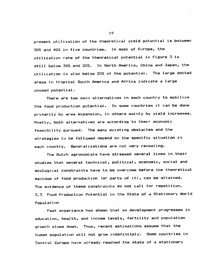
present utilization of the theoretical yield potential is between

30% and 40% in five countries. In most of Europe, the

utilization rate of the theoretical potential in Figure 3 is

still below 30% and 20%. In North America, China and Japan, the

utilization is also below 20% of the potential. The large dotted

areas in tropical South America and Africa indicate a large

unused potential.

There are two main alternatives in each country to mobilize

the food production potential. In some countries it can be done

primarily by area expansion, in others mainly by yield increases.

Mostly, both alternatives are according to their economic

feasibility pursued. The many existing obstacles and the

strategies to be followed depend on the specific situation in

each country. Generalizations are not very revealing.

The Dutch agronomists have stressed several times in their

studies that several technical, political, economic, social and

ecological constraints have to be overcome before the theoretical

maximum of food production (or parts of it), can be attained.

The evidence of these constraints do not call for repetition.

3.3 Food Production Potential in the State of a Stationary World

Population

Past experience has shown that as development progresses in

education, health, and income levels, fertility and population

growth slows down. Thus, recent estimations assume that the

human population will not grow indefinitely. Some countries in

Central Europe have already reached the state of a stationary

-20- -

4J~~~~~~~~~~~~~~~~4C:~~~~~~~~~~~~~~~~~~~~~::

'9~~~~~''

4-I0

00~~~~~~~~~~~~~~~~~~~~~~~~~

CO

0 la

ct o~~~~~~~~~~~~~~~~~~~~~~~

4J~~~~~~~~~~~~~~~~~~~~~~~~~~~~~~~~~~~~~-

0 moo

4-1

WN

co &aQ'6.40 N~~~~~~~~~~~~~~~~~~~~~~~ 4S.a

£4 00*4j~~~~~~~~~~~~~~~~~~~~W

CO to

00~~~~~~~~~~~~~0 Ulm

N0 ~ ~ ~ ~ ~ ~ ~ ~ ~ ~ ~ ~ ~ ~ 0*

H4-O

-4

4£Mto~~~Ioo~ ~ ~~~~~~~~~s

0'9-.

0tI:··

e (U 2.cr o ~ ~ ~ ~ ~ ~ ~ ~ ~ 0 0

No .- £-4 , ·~.

-4B

4 J. · gN~ ~b4 JII

6

4J ~ ~m~Z cx I III I Ir;~do

H 0$ 0~~~~~~~~~~~~~~~~~·

£4~S

21

population. The World Bank (13) has estimated for every country

(excluding countries with a population of less than one million)

the hypothetical size of stationary populations in millions of

people. The nature of these estimations is described by World

Bank as follows: "provide a summary indication of the long-run

implications of recent fertility and mortality trends on the

basis of highly stylized assumptions" (13, p. 282).

The hypothetical size of the stationary population for the

world as a whole is estimated at eleven billion people. The food

production potential was estimated at 49.8 billion tons of grain

equivalents or 4.52 tons of grain equivalents per capita of the

stationary population. The minimum food requirement of the

average person can be set at 3,000 kcal per day or 1.095 X 10-

which corresponds to 332 kg of grain equivalents per year.

Therefore, deducting seed and waste, a per capita production of

more than 400 kg are unconditionally necessary. However, this

level guarantees only the survival and supposes that food is

evenly distributed among the population. Taking into account

that the income distribution is skewed to the left, B00 kg of

grain equivalents would certainly increase safety levels and

minimize the extent of malnutrition among the population.

The maximum food which can be used in an affluent society

which converts grain, roots, tuber and byproducts of industrial

processing into livestock products, alcoholic or non-alcoholic

beverages, and feed for all kinds of pets will not be much above

two tons GE per capita. The theoretical food production

22

potential is, therefore, with 4.5 tons at least two times above

the possible maximum use of food. Utilization rates of 50% and

30%. of the food production potential would still yield 2.2

respectively 1.35 tons of grain equivalents per head of the

stationary world population. It has to be added that the

estimation of the food production potential does not include

livestock products from grazing areas or all food from the sea or

inland waters.

These global considerations have one big disadvantage.

Neither do they take into account the present uneven distribution

of food between countries nor do they indicate what the probable

future food consumption levels will be in each country.

3.4 Food Consumption Levels in Countries at Stationary

Population

Population and income densities per unit of cultivable land

determine in each country the state of technologies and the

attainable food consumption levels. But population growth and

the generation and/or transfer of technical progress does not

grow everywhere at the same rate, or grow in the locationally

required proportions. Therefore, income and food consumption

levels between countries differ enormously. This has been so in

the past and there is no convincing reason to assume that food

consumption in the final state of a stationary world population

would have everywhere the same levels. Therefore, the three

utilization rates of the food production potential (10%, 30%,

50%), as described in Section 3.2 and mapped in Figure 3, are

used in the sequence of the following assessments.

To better identify those countries where food consumption

levels are absolutely insufficient at the final state of a

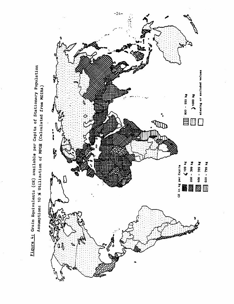
stationary population, six food consumption classes have been

built (Figure 4). The lowest two classes (< 199, 200-400 kg)

represent insufficient food consumption levels, the next two

classes (400-599, 600-799) are medium food consumption levels,

and all classes above 800 kg GE indicate richer states of food

consumption. The dotted areas in Figure 4 are those with a

possible per capita production of more than one ton, which

permits people to strive for a balanced diet. At the low

utilization rate of 10% of the food production potentials all

countries in Oceania, most countries of the Americas, but only a

few in Africa, Asia or Europe would provide more than one ton of

grain equivalents per capita.

The darker shadowed areas characterize those countries where

in the final state less than 400 kg or even less than 200 kg GE

would be available. In both cases, hunger, undernourishment and

malnutrition would prevail. However, if one considers a higher

utilization rate of 30% the remaining countries in America

(except Salvador) and in Europe are moving out of the more

heavily shadowed areas, which represent zones of widespread

hunger, undernourishment, and malnutrition (Figure 5). Likewise,

as in America and Europe, more countries in Africa and Asia

surpass with a 30% utilization rate of the food production

potential, the minimum food requirement stipulated above, at 400

-24-

4-1

CO 4-i

04-4 4-

0m El"

I-.4 4U

oa

Ca

ct~~~~~~~~~~~~~~~~~~~ N

C' I- B '46

C a to

CD~

Cu ~ ~ ~ ~ ~ ~ ~ A

0)0.,.

Swc

Cu u

Cu

0r

5:~ ~ A '

-25-

.10~~~~~~~~~

Aw

'-4 ~ ~ ~ ~ ~ ~ ~ ~ ~ ~~~'

o t

~40 a

CO 4-4

.4 J

co'4

04

id A m4-o 0 0% 0% 0

k~~~~~~~~~~~~~~~~~~~~~~~~~~~~~~~~~0

co

r4O

C7 '-4

o to-

0 44

a~~~~~~O~P"Iti ::

4J~~~~~~~o00 I u

Cuk ~~~~~~'.~~~~~~OO OQ

P. ~8:

04 l

26

kg GE per person. Europe utilizes, doubtlessly, the highest

percentage of its total food production potential (yield

potential X area potential). Some countries are already

approaching the 40% level (Figure 3). Some countries, with their

grain yields, have already surpassed the 50% yield potential

(Figure 2). Weighting both factors and their underlying trends,

it does not seem entirely unfounded to examine what happens to

consumption levels in single countries when one assumes that the

utilization of the food production potential is increased to 50%

(Figure 6). For three countries of Africa (Rwanda, Ethiopia, and

Mauritania) and two in Asia (Nepal and Saudi-Arabia), the food

consumption level would not reach 200 kg/GE/capita. Saudi Arabia.

will certainly have like at present the purchasing power to buy

from the international market. In Mauritania and Nepal the not

calculated livestock economy based on ruminants plays a large

role. Therefore, the net effects would be less than calculated.

Less than 400 kg/GE/capita would be available in Afghanistan,

Bangladesh, Niger, and Nigeria. The first group of countries

embraces 348 millions and the second counts 1,188 millions of the

stationary population or 3.2% and 10.8% respectively of the

world's total.4

Before one tries to assess the present and possible future

situation in those countries, one has to be aware that the

estimations are based on several assumptions.

1. For the sake of simplifying the calculations, no trade in

food and agricultural commodities between surplus and

-27-

o~ ~~~~~~o

4-3~~~~~~~~~~~~~~~~~~~~~~~~~~~~~~~~~~~~~~~-

0 a0

CO 4-

H) 0

o

0 c

MI

+)~~~~~~~~~~~~~~~~~~~~~~~~~~~~~~~~~~~~~~~~~~~~~~~~~~~~~~~C

ao

K

0U a~

co W A m

H r. 0~~~~~~~~~~~~~~~~~~~~~% . .%0% C-4 .0 (% 0~~~~~~~~~~~~~~ co C

4 -co ) U

H ~ ~ ~ ~ ~ ~ ~ H ;

00- t Pc4

*,vlo~~~~ ~~~~~~~~~~~ wa w u0 K M K K~~~~~~~~~~~~~~~~~~i

ca ~ ~ ~ ~ ~ ~ ~ ~ ~ ~ ~ ~ ~ ~ ~~~~0 0%0%

-U H····... ·. ~~~~~~~ U~~I~~ 1111111111...·:: ··:··i~~~~~~~~~~~~~~~l::.;:;.;·. ~~~~~~~7S.

0-4 0o c~~~~~~~~~~~~~~~~~~~~~~~~~~~~~~~~~~~~~0

(42

00·

0'

Po~~Qh '~" P.

28

deficit countries has been assumed.

2. The present rigidity of national boundaries prevents

large international migrations of agricultural people

from taking place. To give an example: From the

"overcrowded" Rwanda, people could migrate to

neighbouring countries like Tanzania or Zaire which will

use, in the final state, a much lower level of their food

production potential. Whether larger migrations finally

will take place seems at present a very speculative

reflection.

3. As the recent experience shows (13), declines of

population growth will probably be stronger than the

present estimations indicate. The various governments'

population policies initiated in the last decade in

developing countries will, with high probability, become

with some culturally determined delays more effective in

the future.

4. The accuracy of the estimations at country levels based

on MOIRA's soil and climate inventory should not be

overvalued. There may be, in parts of the countries,

overestimates as well as underestimates of the food

production potential. It is assumed that they cancel

each other out.

5. The final state of a stationary world population will

occur under present norms of population growth at the end

of the next century. However, in most of the developing

29

countries, this is happening 50 years earlier. That

gives ample time to adjust the resources to the

requirements in the poorest of the food-deficit

countries. However, even after all adjustments have been

made, the food consumption levels in the final stationary

state of the world population will probably remain uneven

as today. But it should be a lesser problem to raise the

standards of food consumption in the poorest countries.

4. Conclusion

The present very hypothetical calculations and estimations

certainly do not have the state of accuracy one would wish to

have. The presented results suggest that the world is not, even

in the very long-run, running out of food. The present wisdom

permits the conclusion that there will be no unconstrained

population growth. Therefore, if man continues to use all his

wit and sagacity, he has very good chances to produce all the

food he really needs.

Endnotes

'The Dutch agronomists framed the food production potentialof the earth (or the theoretical maximum of food production) asthe (Absolute) Maximum Production of Grain Equivalents (MPGE).If not expressively referred to MOIRA, the three terms are usedinterchangeably.

=In my review of the MOIRA-Study, I tried to deal with bothparts of the model (11). Despite the importance of the book, themultidisciplinary approach was obviously a hindrance for broaderand deeper reviews in agricultural economic journals. Theeconomists used the agronomic part of the rather complex economicMOIRA-model to examine whether the food production potentialwould permit to provide people in 106 geographical units(countries) with sufficient food in the year 2009 (1, pp. 306-326). Under the various assumptions of the model the simulatedresults for aggregated regions showed that in the year 2009 overone billion people would not reach the minimum food standard setat 300 kg grain equivalents per capita unless massive food aid orcapital transfers would be initiated.--However, the concern inthis study is not the effect of specific policies in a fixed timeperiod for highly aggregated regions. The aim is to assess andto compare for single countries the food production potentialwith estimated stationary populations. Therefore, our approachis much more modest.

'The standard crop is conceived as a C3 plant, "with theproperties of a cereal" (1, p. 27). The ratio of straw to grainis calculated at 1:1. It is known that some C4 plants, likesugarcane, have higher photosynthetic performances and arenormally grown in the warmer climates. However, the optimal mixof crops at each location will finally be determined by theprofitability of and the demand for crops and not by theirphotosynthetic efficiency. Further, one has to be aware that theconceived "standard crop" is a theoretical concept developed tocover all food crops and all regions of the world. Because ofcereals' worldwide importance in cultivation and human food, theyare used in this study as an indicator for the variousutilization rates of the food production potential or the MPGE.

4 The listed countries which have probably at a 50%utilization rate of the food production potential insufficientfood consumption levels if the present trends persist are alsodescribed as critical countries in the FAO/IIASA study (8). Thisseems to vindicate the planimetric calculations made here.

31

References

(1) Buringh, P., H. D. F. van Heemst and G. F. Staring,Computation of the Absolute Maximum Food Productionof the World. Wageningen 1975. Note: The resultswere later published in Chapter 2 of: H. Linnemann,J. de Hoogh, M. A. Keyzer and H. D. F. van Heemst

with contributions by R. F. Broisma, F. N. Bruinsma,P. Buringh, G. F. Staring, C. T. De Wit: MOIRA(Model of International Relations in Agriculture).New York, Oxford 1979. Here only quoted from andreferred to as MOIRA.

(2) Egorov, V. V., Prirodno-selskokhoziastvennoeRaionirovanie Zemel'-noao Fonda SSSR. Moskva 1975.

(3) FAO/IIASA/UNFPA, Potential Population-SupportinqCapacities of Lands in the Developing World.(Technical Report of Project-FPA/INT/513) Rome 1982.

(4) Lieth, H., Basis und Grenze fur die Menschheits-entwicklung: Stoffproduktion der Pflanzen. Umschau,Vol. 46 (1972), pp. 169-174.

(5) Lieth, H., Uber die Primarproduktion derPflanzendecke der Erde. Anqewandte Botanik, Vol. 46(1972), pp. 169-174.

(6) Lieth, H., Historical Survey of Primary ProductivityResearch. In: Lieth, H. and R. H. Whittaker (Eds.),Primary Productivity of the Biosphere. (EcologicalStudies, 14). Berlin, Heidelberg, New York 1975, pp.7-16.

(7) Rauner, F. L., Klimat i Urozhainost' Zernovykh Kul'tur. Moskva 1981.

(8) Shah, M. and G. Fischer, People, Land, and FoodProduction: Potentials in the Developing World.Options 1984, 2, pp. 1-5.

(9) Thomsen, Margot, Untersuchunqen zur langfristigenErtraqsentwicklung in Schleswiq-Holstein.Agricultural science dissertation (agriculturaleconomics). Kiel 1986.

(10) Weber, A., Welternahrungswirtschaft. In:Handworterbuch der Wirtschaftswissenschaft, Bd. 9.Gottingen, Stuttgart, Tubingen 1980, pp. 612-637.

(11) Weber, A., Book Review of MOIRA (Model of

32

International Relations in Agriculture). In:Quarterly Journal of International Agriculture, Vol.20 (1981), pp. 101-110.

(12) Wit, De, C. T., Photosynthesis of Leaf Canopies.(Agricultural Research Reports, No. 663). Wageningen1965.

(13) World Bank, World Development Report 1984.

APPENDIX

Table 1: Maximum Production of Grain Equivalents(MPGE), Potentials of Agricultural Land andYields (MOIRA)

Table 2: Present Grain Yield Levels (1981/83) asFraction of the Maximum Production of GrainEquivalents per Hectare of PotentialAgricultural Land (MPGE/PAL)

Table 3: Grain Equivalents (GE) Available per Capitaof Stationary Population at VariousUtilization Rates of the Food ProductionPotential

Table 4: The Hypothetical Size of the StationaryPopulation

-34-

Table 1: Maximum Production of Grain Equivalents (MPGE),Potentials of Agricultural Land and Yields (MOIRA)

(1) (2) (3) (4) (5) (6)COUNTRY MPGE PAL MPGE/PAL (t/ha) Number of

(10 6 t) (106 ha) Min. Max. Med. Regions

Europe

Norway 15.0 2.5 0.0** 6.7 6.o 3Sweden 81.4 12.2 5.2 7.9 6.7 3Finland 52.5 9.6 0.0* 7.2 5.5 4Denmark 20.9 2.0 10.4 10.4 10.4*** 1Ireland 27.1 2.6 7.3 10.9 10.4 2United Kingdom 126.3 10.6 7.3 136 11.9 3Netherlands 24.3 1.9 10.4 14.1 12.8 2Belgium 26.7 2.0 10.4 14.1 13.4 4France 372.9 27.0 10.0* 23.0 13.8 8Germany F.R. 148.5 12.2 10.0* 14.1 12.2 5German D.R. 63.4 6.0 10.4 10.9 10.6 2Poland 186.6 18.0 7.2 10.9 10.4 5Czechoslovakia 62.1 5.2 10.0* 14.0 11.9 4Switzerland 2.1 0.2 10.0* 10.0* 10.O*** 1Austria 26.3 2.0 10.0* 13.4 13.2 4Hungary 42.6 3.1 12.8 14.0 13.7 2Portugal 51.7 4.0 10.8 15.3 12.9 3Spain 272.9 21.3 10.8 14.2 12.8 4Italy 131.9 10.0 6.7 21.2 13.2 5Yugoslavia 135.3 10.2 9.2 15.5 13.3 4Romania 106.1 9.1 8.3 14.0 11.7 6Albania 16.7 1.1 15.5 15.5 15.5*** 1Bulgaria 57.3 5.2 9.2 12.8 11.0 4Greece 51.8 3.6 9.2 19.5 14.4 3U.S.S.R.(Eur. Part) 1917.9 204.2 0.0** 19.5 9.4 14U.S.S.R(Asian Part) 2371.5 271.0 0.0** 12.7 8.8 16U.S.S.R. (Tot-i) 4289.4 475.4 0.0** 19.5 9.0 30

Asia

Turkey 144.7 11.7 6.8 19.5 12.4 5Syria 66.6 8.9 6.8 14.7 7.5 3Iraq 159.7 10.5 6.8 20.8 15.2 4Saudi Arabia 3.9 0.2 0.0+ 30.0++ 19.5 1Iran 201.9 39.5 4.3 11.1 5.1 3Afghanistan 52.3 10.4 4.3 11.1 5.0 3Pakistan 402.4 21.9 0.0* 24.2 18.4 6India 3027.1 138.6 0.0* 29.9 21.8 9Nepal 3.3 0.6 5.2* 5.2* 5.2*** 1Sri Lanka 66.5 3.0 22.0 22.0 22.0*** 1Bangladesh 255.7 8.5 29.9 29.9 29.9*** 1Mongolia 114.5 35.2 2.0 5.8 3.3 3China 3377.7 305.1 0.0* 28.7 11.1 13Burma 361.1 19.9 5.2* 28.7 18.1 3Lao 140.9 7.9 14.8 21.0 17.8 2Thailand 510.8 23.5 14.8 28.7 21.7 4Kampuchea 199.7 9.1 21.0 28.7 21.9 2Vietnam 222.6 11.0 14.8 28.7 20.2 4Korea (Rep.) 4.0 0.4 10.7* 10.7* 10.7*** 1Korea Peoples Rep.) 6.9 o.6 10.7* 10.7* 10.7*** 1Japan 298.0 20.8 14.3 14.3 14.3*** 1Malaysia 248.0 14.3 17.3 17.3 17.3*** 1Philippines 134.2 8.0 16.8 16.8 16.8*** 1Indonesia 1818.9 93.2 16.8 25.2 19.5 4_ _ _ _ _~~~

-35-

Table 1 (ontinued)(D(1) (2) (3) 4) ( 6

COUNTRY~ MPGE PAL MPGE/PAL (t/ha) Number of

(106 t) (106 ha) Min. Max. Med. RegionsAfrica

Morocco 86.6 13.9 0.0** 9.7 6.2 3Algeria 95.6 18.1 0.0** 9.7 5.3 4Tunesia 35.3 4.8 0.0** 9.7 7.4 4Libya 36.8 5.2 0.0** 7.0 7.0 2Egypt 133'0 4.9 0.0** 28.0 28.0 2Mauritania 2.7 0.8 0.0** 3.3 3.3 2Senegal 58.3 3.5 0.0** 16.9 16.9 2Mali 208.0 22.7 0.0** 19.7 9.2 4Burkina Faso 116.1 10.8 0.4 11.0 10.8 2Chad 103.4 19.1 O.0** 16.4 5.4 4Sudan 417.3 70.1 0.0** 21.5 6.0 7Niger 301.5 12.7 0.0** 11.0 2.4 3Guinea 210.1 11.8 11.0 19.7 17.8 3Sierra Leone 30.9 1.8 16.9 16.9 16.9*** 1Liberia 58.3 3.5 16.9 16.9 16.9*** 1Ivory Coast 303.0 15.7 11.0 19.7 19.3 3Ghana 146.4 10.2 11.0 19.7 14.4 4Togo 36.2 2.9 11.0 16.4 12.5 2Benin 52.7 4.4 11.0 16.4 12.0 2Nigeria 412.7 33.9 0.4 17.6 12.2 4Cameroon 222.9 14.7 11.0 17.6 15.2 3Centr. Afr. Rep. 314.7 19.9 11.0 16.4 15.8 2Gabon 162.3 9.7 16.4 17.6 16.7 3Congo 251.8 13.9 16.4 25.5 18.1 5Zaire 1837.0 98.0 16.4 25.5 18.7 8Ethiopia 91.7 10.7 0.0** 17.2* 8.6 5Somalia 86.7 12.2 0.0** 14.7 7.1 3Uganda 196.4 9.1 21.5 21.5 21.5*** 1Kenya 267.3 14.3 O.O** 21.5 18.8 3Rwanda 24.5 1.1 21.5 21.5 21.5*** 1Burundi 24.5 1.1 21.5 21.5 21.5*** 1Tanzania 806;0 37.9 14.7 21.5 21.3 2Angola 995.8 61.0 3.1 20.7 16.3 6Zambia 713.0 37.4 17.3 20.7 19.1 3Malawi 48.0 2.7 17.6 17.6 17.6*** 1Mozambique 632.7 33.2 17.6 20.7 19.1 3Namibia 133.7 14.4 O.0** 17.3 9.4 4Botswana 251.9 21.3 3.9 19.8 11.8 3Zimbabwe 268.6 14.8 17.3 20.7 18.1 4Swaziland 18.3 0.9 19.8 19.8 19.8*** 1Lesotho 32.0 1.6 19.8 19.8 19.8*** 1South Africa 480.6 32.1 3.1* 19.8 15.0 4Madagascar 335.0 25.2 9.0 17.7 13.3 2

North and Central America

Canada 1218.2 173.5 0.0** 8.8 7.0 8U.S.A. 4292.5 371.6 5.2 22.6 11.6 17Mexico 839.1 53.6 5.2 21.2 15.7 10Guatemala 60.8 2.7 21.2 24.6 22.5 3El Salvador 21.2 0.9 24.6 24.6 24.'6*** 1Honduras 93.2 3.9 23.8* 24.6 23.9 3Nicaragua 134.5 5.5 23.8* 24.6 24.5 2Costa Rica 74.3 3.0 24.6 24.6 24.6*** 1Panama 100.9 4.1 24.6 24.6 24.6*** 1Cuba 92.3 4.4 21.2 21.2 21.2*** 1Haiti 31.9 1.3 24.6 24.6 24.6*** 1Dom. Rep. 79.6 3.3 24.6 24.6 24.6*** 1Jamaica 10.7 0.4 2. u .- +.O 44.u*W

-36-

Table- 1 (continuec)

COUNTRY PGE PAL MPGE/PAL (t/ha) Number of(106t) (106 ha) Min. Max. Med. Regions

boutn America

Venezuela 64o.i 29. i7.1 24. 2-'.9 4G~uyana ,'i.O uo.o 't.'l 24.4 21.4 3French Guyana 39.6 1.9 17.1 24.4 20.8 2Suriname 93.2 4.4 17.1 24.4 21.2 2Columbia 905.0 38.5 18.7* 24.7 23.5 6Ecuador 75.8 3.2 3.0* 24.7 23.7 5PeruBolivia 550.4 30.7 1.0* 23.5* 17.9 6Bolivia 562.8 33.2 1.0* 23..5* 17.0 9

Paraguay 293.2 18.0 11.4 20.7 16.3 6Arntina 6534.8 348.3 12.6 25.6 18.8 16Cgentina 1095.5 90.1 2.0* 19.2 12.2 9Chile 59.7 6.2 1.0* 13.4* 9.6 4Uruguay 114.6 4.6 24.8 25.6 24.9 2

Oceania

Australia 1942.0 201.3 0.0** 21.3 9.6 19Papua New Guinea 284.4 16.9 16.8 16.8 16.8*** 1New Zealand 139.0 10.7 1.3* 16.6 13.0 4FijiSolomon Is.New Caledonia 277.0 13.7 20.2 20.2 20.2*** 1Vanuatu

World 49918 3714 0.0** 30.0++ 13.4 222

* Region C (High Mountain) The planimetrically derived values areRegion D (Desert, Tundra) strongly distorted because theshare of arable land is very+ ~smaell.*** Minimax=Maximax, because only one -egion, in some casessmall deviation from average MPGE/PAL+ without Irrigation++ only with Irrigation

Source: MOIRA. - Owncalculation.

-37-

Table 2: Present Grain Yield Levels (1981/83) as Fraction of the Maximum Productionof Grain Equivalents per Hectare of Potential Agricultural Land (MPGE/PAL)

(1) (2) (3) (4) (5)Grain- in % of Arable in % of in % of

COUNTRY yield yield- land land- total(kg) potential (1000 ha) potential potential

a)

Europe

Norway 3606 0.60 840 0.34 0.20Sweden 3798 0.57 2982 0.24 0.14Finland 2723 0.50 2368 0.25 0.13Denmark 4121 0.40 2645 1.00** 0.40Ireland 4986 0.48 972 0.37 0.18United Kingdom 5263 0.44 6992 0.66 0.29Netherlands 6355 0.50 862 0.45 0.23Belgium 5141 0.38 831 0.42 0.16France 4862 0.35 18766 0.70 0.35Germany F.R. 4623 0.38 7466 0.61 0.23German D.R. 3834 0.36 5008 0.83 0.29Poland 2611 0.25 14829 0.82 0.21Czechoslovakia 4072 0.34 5170 0.99 0.34Switzerland 5100 0.51 412 1.00** 0.51Austria 4558 0.35 1583 0.79 0.28Hungary 4839 0.35 5305 1.00** 0.35Portugal 962 0.07 3550 1.00** 0.07Spain 1773 0.14 20498 0.96 0.13Italy 3607 0.27 12323 1.00** 0.27Yugoslavia 3846 0.29 7838 0.77 0.22Romania 3178 0.27 10532 1.00** 0.27Albania 2754 0.18 708 0.64 0.12Bulgaria 4144 0.38 4153 0.80 0.30Greece 3162 0.22 3962 1.00** 0.22U.S.S.R. 1448 0.15 232282 0.49 0.07

Asia

Turkey 1915 0.15 27452 1.00** 0.15Syria 1039 0.14 5683 0.64 0.09Iraq 911 0.06 5450 0.52 0.03Saudi Arabia 1407 0.07 1129 1.00** 0.07Iran 1207 0.24 13700 0.35 0.08Afghanistan 1341 0.27 8054 0.77 0.21Pakistan 1664 0.09 20410 0.93 0.08India 1435 0.07 168370 1.00** 0.07Nepal 1687 0.32 2331 1.00** 0.32Sri Lanka 2429 0.16 2171 0.72 0.12Bangladesh 2001 0.07 9133 1.00** 0.07Mongolia 1036 0.31 1262 0.04 0.01China 3399 0.31 100897 0.33 0.10Burma 2891 0.16 10068 0.51 0.08Lao 1495 0.08 888 011 0.01Thailand 1960 0.09 19026 0.12 0.01Kampuchea 900 0.04 3046 0.33 0.01Vietnam 2332 0.12 7105 0.65 0.08Japan 5300 0.37 4830 0.23 0.09Malaysia 2857 0.17 4338 0.30 0.05Philippines 1699 0.10 11180 1.00** 0.10Indonesia 3165 0.16 19930 0.21 0.03

-38-

Table 2 (continued)

(1) (2) (3) (4) (5)Grain- in % of Arable in % of in % ofCOUNTRY yield yield- land land- total(kg) potential (1000 ha)potential potential

a)

Africa

Morocco 941 0.15 8394 0.60 0.09Algeria 596 0.11 7509 0.41 0.05Tunesia 882 0.12 4681 0.98 0.12Libya 432 0.06 2091 0.40 0.02Egypt 4254 0.15 2470 0.50 0.08Mauritania 423 0.13 195 0.24 0.03Senegal 625 0.04 5225 1.00** 0.04Mali 576 0.06 2053 0.09 0.01Burkina Faso 541 0.05 2633 0.24 0.01Chad 422 0.08 3150 0.16 0.01Sudan 603 0.10 12448 0.18 0.02Niger 408 0.17 3560 0.28 0.05Guinea 867 0.05 1574 0.13 0.01Sierra Leone 1397 0.08 1769 0.98 0.08Liberia 1206 0.07 371 0.11 0.01Ivory Coast 672 0.03 3958 0.25 0.01Ghana 799 0.06 2765 0.27 0.02Togo 875 0.07 1426 0.49 0.03Benin 621 0.05 1802 0.41 0.02Nigeria 696 0.06 30410 0.90 0.05Cameroon 835 0.05 6950 0.47 0.02Centr. Afr. Rep. 538 0.03 1958 0.10 0.01Gabon 1593 0.10 452 0.05 0.01Congo 539 0.03 672 0.05 0.01+Zaire 822 0.04 6406 0.07 0.01+Ethiopia 1280 0.15 13930 1.00** 0.15Somalia 6810 0.10 1066 0.09 0.01Uganda 1565 0.07 6030 0.66 0.05Kenya 1460 0.08 2310 0.16 0.01Rwanda 1135 0.05 1010 0.92 0.05Burundi 1175 0.05 1306 1.00** 0.05Tanzania 1147 0.05 5190 0.14 0.01Angola 474 0.03 3500 0.06 0.01+Zambia 1706 0.09 5158 0.14 0.01Malawi 1165 0.07 2332 0.86 0.06Mozambique 478 0.03 3080 0.09 0.01+Namibia 378 0.04 660 0.05 0.01+Botswana 192 0.02 1360 0.06 0.01+Zimbabwe 1157 0.06 2680 0.18 0.01Swaziland 1193 0.06 139 0.15 0.01Lesotho 840 0.04 298 0.19 0.01South Africa 1608 0.11 13620 0.42 0.05Madagascar 1648 0.12 3006 0.12 0.01

-39-

Table 2: (continued)

(i1 ) 1d) (Do t~j j4)

COUNTRY Grain- in % of Arable in % of in % ofyield yield- land land- total(kg) potential (1000 ha) potential potential(kg) a)

North and Central America

Canada 2351 0.34 46201 0.27 0.09U.S.A. 4076 0.35 190270 0.51 0.18Mexico 2272 0.14 23525 0.44 0.06Guatemala 1459 0.07 1786 0.66 0.05El Salvador 1558 0.06 725 0.81 0.05Honduras 1398 0.06 1767 0.45 0.03Nicaragua 1719 0.07 1262 0.23 0.02Costa Rica 2079 0.08 626 0.21 0.02Panama 1009 0.04 582 0.07 0.01+Cuba 2336 0.11 3213 0.73 0.08Haiti 965 0.04 897 0.69 0.03Dom. Rep. 3579 0.15 1442 0.44 0.07Jamaica 1527 0.06 267 0.67 0.04

South America

Venezuela 2015 0.09 3757 0.13 0.01Columbia 2477 0.11 5676 0.15 0.02Ecuador 1793 0.08 2512 0.79 0.06Peru 2156 0.12 3516 0011 0.01Bolivia 1203 0.07 3375 0.10 0.01Paraguay 1358 0.03 1940 0.11 0.01+Brazil 1593 0.08 73985 0.21 0.02Argentina 2353 0.19 35450 0.39 0.07Chile 2149 0.22 5528 0.89 0.20Uruguay 1813 0.07 1448 0.31 0.02

Oceania

Australia 1280 0.13 44878 0.22 0.03Papua New Guinea 1442 0.09 372 0.02 0.01New Zealand 4573 0.35 461 0.04 0.01

** Calculated share of utilisation of potential land is higher than 1;therefore correction to maximum share 1.00.

+ smaller than 0.005,a) including permanent cultures,

Source: MOIRA. - FAO Production Yearbook Vol. 38, Rome 1984.Own calculations,

-40-

Table 3: Grain Equivalents (GE) Available per Capita of Stationary Populationat Various Utilization Rates of the Food Production Potential

(1) (2) (3) (4) (5)COUNTRY Stetionary MPGE/Capita/kg kg GE per capitapopulation of stationarypopulation

(Mill.) (100%) 10%MPGE 306%MPGE 50%MPGE

Europe

Norway 4 3750 375 1125 1875Sweden 8 10125 1013 3038 5063Finland 5 10600 1060 3180 5300Denmark 5 4200 420 1260 2100Ireland 6 4500 450 1350 2250United Kingdom 59 2136 214 641 1068Netherlands 15 1600 160 480 800Belgium 10 2700 270 810 1350France 62 5210 521 1563 2605Germany F.R. 54 2759 276 828 1380German D.R. 18 3500 350 1050 1750Poland 49 3816 382 1145 1908Czechoslovakia 20 3100 310 930 1550Austria 8 3250 325 975 1625Hungary 12 3583 358 1075 2866Portugal 14 3714 371 1114 1857Spain 51 5353 535 1606 2677Italy 57 2315 232 695 1158Yugoslavia 29 4655 466 1397 2328Romania 31 3419 342 1026 1710Albania 6 2833 283 850 1417Bulgaria 10 5700 570 1710 2850Greece 12 4333 433 1300 2167U.S.S.R. 377 11377 113L 3412 5688

Asia

Turkey 111 1306 131 392 653Syria 42 1595 160 479 798Iraq 68 2353 235 706 1177Saudi Arabia 62 65 7 20 33Iran 159 1270 127 381 635Afghanistan 76 684 68 205 342Pakistan 377 1066 107 320 532India 1707 1773 177 532 887Nepal 71 42 4 13 21Sri Lanka 32 2094 209 628 1047Bangladesh 454 564 56 169 282Mongolia 5 23000 2300 6900 11500China 1461 2312 231 694 1156Burma 115 3139 314 942 1570Lao 19 7421 742 2226 3711Thailand 111 4604 460 1381 2302Vietnam 171 1304 130 391 652Japan 128 2328 233 698 1164Malaysia 33 7515 752 2255 3758Philippines 127 1055 106 317 528Indonesia 370 4916 492 1475 2458

-41-

Table 3: (continued)

(1) (2) (3) (4) (5)COUNTRYCOUNTRY Stationary MPGE/Capita/kg kg GE per capita

population of stationary(Mill.) pop ulation 109MPGE 30%MPGE 50%MPGE

Africa

Morocco 70 1243 124 373 621Algeria 119 807 81 242 403Tunisia 19 1842 184 553 921Libya 21 1762 176 529 881Egypt 114 1202 120 360 601Mauritania 8 375 38 113 188Senegal 36 1611 161 483 806Mali 42 4976 498 1493 2488Burkina Faso 35 3314 331 994 1657Chad 22 4682 468 1405 2341Sudan 112 3723 372 1117 1862Niger 40 775 78 233 388Guinea 28 7500 750 2250 3750Sierra Leone 16 1938 194 581 969Liberia 12 4833 483 1450 2417Ivory Coast 58 5224 522 1567 2612Ghana 83 1759 176 528 880Togo 17 2118 212 635 1059Benin 23 3609 361 1083 1804Nigeria 618 668 67 200 334Cameroon 65 3431 343 1029 1715Centr. Afr. Rep. 13 24231 2423 7269 12115Congo 10 25200 2520 7560 12600Zaire 172 10680 1068 3204 5340Ethiopia 231 398 40 119 199Somalia 23 3783 378 1135 1891Uganda 89 2202 220 661 1101Kenya 153 1745 175 524 873Rwanda 47 532 53 160 266Burundi 27 926 93 278 463Tanzania 117 6889 689 2067 3444Angola 44 22636 2264 6791 11318Zambia 37 19270 1927 5781 9635Malawi 48 1000 100 300 500Mozambique 82 7720 772 2316 3860Zimbabwe 62 4339 434 1302 2169Lesotho 7 4571 457 1371 2280South Africa 123 3910 391 1173 1955Madagascar 54 6204 620 1861 3102

-42-

Table 3: (continued)

(1) (2) (3) (4) (5)Stationary MPGE/Capita/kg kg GE per capita

COUNTRY population of stationary(Mill.) population 10%MPGE 3096MPGE 50%MPGE(M ll.) (100%)

North and Central America

Canada 33 36909 3691 11072 18454U.S.A 292 14702 1470 4411 7351Mexico 199 4216 422 1265 2109Guatemala 25 2440 244 732 1220El Salvador 17 1235 124 371 618Honduras 17 5471 547 1641 2735Nicaragua 12 11250 1125 3375 5625Costa Rica 5 14800 1480 4440 7400Panama 4 25250 2525 7575 12625Cuba 15 6133 613 1840 3067Haiti 14 2286 229 686 1143Dom. Rep. 15 5333 533 1600 2667Jamaica 4 2750 275 825 1375

South America

Venezuela 46 13913 1391 4174 6956Columbia 62 14597 1460 4379 7298Ecuador 27 2815 282 844 1407Peru 49 11224 1122 3367 5612Bolivia 22 25591 2559 7677 12795Paraguay 8 36625 3663 10988 18313Brazil 304 21496 2150 6449 10748Argentina 54 20296 2030 6089 10148Chile 21 2857 286 857 1429Uruguay 4 28750 2875 8625 14375

Oceania

Australia 21 92476 9248 27743 46623Papua New Guinea 10 28400 2840 8520 14200New Zealand 4 34750 3475 10425 17375

Source: MOIRA.- World Bank, World Development Report 1984.-Own calculations.

-43-

Table 4: The Hypothetical Size of the Stationary Population

Country Categories Millions

Low income countries 5,863

Middle income countries 2,397

Upper-middle income coutries 1,338

High income oil exporters 96

Industrial market economies 828

East European nonmarket economies 523

World 11,039

Source: World Bank, World Development Report 1984.