p-v-l deep: a big data analytics solution for now-casting
TRANSCRIPT
P-V-L Deep: A Big Data Analytics Solution for Now-casting in
Monetary Policy
Maryam Hajipour Sarduie
Ph.D. Candidate, Department of Information Technology Management, Science and Research Branch,
Islamic Azad University, Tehran, Iran. E-mail: [email protected]
Mohammadali Afshar Kazemi*
*Corresponding author, Associate Prof., Department of Industrial Management, Science and Research
Branch, Islamic Azad University, Tehran, Iran. E-mail: [email protected]
Mahmood Alborzi
Associate Prof., Department of Information Technology Management, Science and Research Branch,
Islamic Azad University, Tehran, Iran. E-mail: [email protected]
Adel Azar
Prof., Department of Management, Tarbiat Modares University, Tehran, Iran. E-mail:
Ali Kermanshah
Associate Prof., Department of Management, Sharif University of Technology, Tehran, Iran. E-mail:
Abstract
The development of new technologies has confronted the entire domain of science and industry with
issues of big data's scalability as well as its integration with the purpose of forecasting analytics in its
life cycle. In predictive analytics, the forecast of near-future and recent past - or in other words, the
now-casting - is the continuous study of real-time events and constantly updated where it considers
eventuality. So, it is necessary to consider the highly data-driven technologies and to use new methods
of analysis, like machine learning and visualization tools, with the ability of interaction and connection
to different data resources with varieties of data regarding the type of big data aimed at reducing the
risks of policy-making institution’s investment in the field of IT. The main scientific contribution of
this article is presenting a new approach of policy-making for the now-casting of economic indicators
in order to improve the performance of forecasting through the combination of deep nets and deep
Journal of Information Technology Management, 2020, Vol.12, No.4 23
learning methods in the data and features representation. In this regard, a net under the title of P-V-L
Deep: Predictive Variational Auto Encoders - Long Short-term Memory Deep Neural Network was
designed in which the architecture of variational auto-encoder was used for unsupervised learning,
data representation, and data reconstruction; moreover, long short-term memory was adopted in order
to evaluate now-casting performance of deep nets in time-series of macro-econometric variations.
Represented and reconstructed data in the generative network of variational auto-encoder to determine
the performance of long-short-term memory in the forecasting of the economic indicators were
compared to principal data of the net. The findings of the research argue that reconstructed data which
are derived from variational auto-encoder embody shorter training time and outperform of prediction
in long short-term memory compared to principal data.
Keywords: Big data analytics, Deep learning, Now-casting, monetary policy.
DOI: 10.22059/jitm.2020.293071.2429 © University of Tehran, Faculty of Management
Introduction
Financial and monetary policies are among the most important forms of government
intervention in the macro-economic direction, and especially monetary policy is one of the
regulatory tasks of the world's central banks. The approach of most central banks in the last
few decades can be divided into three important periods, based on the turning point of the
2008-2009 crisis:
Pre-crisis; with features
o Lagging distribution of macro-economic indicators and the traditional use of
simple foresight models by policy-making institutions
o Concentration on aggregated data used at the level of central bank balance sheets
o Focus on deductive/ inference approach
Crisis; with features
o Distortions and lack of equilibrium economic
o Reveal the deficiency of deductive models due to inability and confrontation of
accepted financial models with a huge amount of data contributing eventually to
decrease of accuracy in forecasting
o Complexity in data analytics because of non-linear relations
o Data tsunami and the emergence of the big data paradigm due to the rapid
development of computer and internet networks, and the formation of new
sources of information and digital data
P-V-L Deep: A Big Data Analytics Solution for Now-casting in Monetary Policy 24
o Focus on topics, especially those relating to cause and effects as well as
contractual reward in models that are easy to interpret due to access to massive
data resources
o Focus on the inductive approach and not to pay attention to theoretical
generalizations
Post-Crisis; with features
o Real-time and immediate assessment of the economic situation
o Focus on the data-driven approach including technologies, techniques, methods,
and tools
o Focus on the abduction approach (the hybrid approach inductive and deductive)
Big data is a transformative paradigm that its trend analyses and its turning points lead
to an improvement in the outlining of real-time conditions of economy through data-driven
decisions. One of the lessons of the financial crisis was to draw the attention of policy makers
to more detailed data and the use of data-driven approaches in now-casting of economic
indicators. Therefore, pondering over big data paradigm, due to its robust potential in
resolving many now-casting struggles, moves researches from usage of structural equations
towards innovations and advancements in new techniques of AI in a way that in order to
confront this paradigm shift, policy-making institution attempts to reinforce the agility of big
data processes aimed at accelerating to present business values.
Among all institution, it seems that banks and financial institutes are closer to now-
casting because of more timely and accurate forecasting (Varian, 2018; Lu, 2019; Yasir, et al.,
2020; Ostapenko, 2020). Now-casting is also one of the standard activities of central banks so
that they use a variety of models in order to achieve a proper comprehension of economic
changes in the future and in time a head.
Thus, the focus of modern econometric analysis is on big data, and in particular on now-
casting, based on the behavior of economic variables, which does not rely on economic
theories and is based solely on non-linear and complex relationships of data. In this way, the
use of machine learning techniques has led to a significant improvement in predictions.
Hence, now-casting moves from causal inference towards the field of machine learning,
because of its data-driven nature.
So, the main problem of this research is to determine the model of the eventuality and
real-time data aligned with the now-casting of monetary policies.
Accordingly, central banks need data-driven policy-making in order to respond to its
current responsibility on now-casting and accurate evaluation of the current situation, the
Journal of Information Technology Management, 2020, Vol.12, No.4 25
possibility of corrective measures and interventions, early monitoring of events, and the
effects of measures, establishing new policy perspectives in the policy-making institution.
Therefore, it is necessary to develop a general strategy to enter the conceptual,
technical, and policy areas in the application of emerging data-driven technologies in the
context of supervision and macro-economics.
According to the United Nation, big data is attractive for the policy-making domain as
well as the academic area (Njuguna, 2017). Establishing monetary stability and bank
supervision are necessary measures for policy-making institutions to make policies. It
signifies the development of big data boundaries (scopes) as relevant data resources. If these
resources can specifically help to identify the economy’s trends and milestones, they can
provide a more realistic image of the economy and alarming, real-time indicators through
complementary and more on-time information for policy-making institutions compared to
conventional tools. Consequently, countries will experience an important improvement in
economic stability over time (Nymand-Andersen, 2016). Thus, the importance of big data
analytics and economic condition’s now-casting, in the recent universal crisis in which the
delay of key indicators’ release in macro-econometrics is considered as an obstacle, for
policy-making institutions and economic activists is undeniable. While the whole universe is
experiencing a burst of data volume, variety and velocity due to the emergence of new
technologies and digital tools (Global Pluse, 2013). In these conditions, data-driven decisions
and data-driven now-casting models based on real-time enable managers to propel monetary
policies in the right path by their corrective measures conventional and unconventional in
addition to making macro-prudential and financial policies as well as providing investment
strategies (Bragolia & Modugno, 2016).
Recently, data-driven forecasting modeling is applied in different areas including
monetary policy (Yasir, et al., 2020; Ostapenko, 2020; Lu, 2019), speech and audio
processing (Girin, Hueber, Roche, & Leglaive, 2019), text modeling (Li, Li, Lin, Collinson, &
Mao, 2019), image analysis and recognition (Karray, Campilho, & Yu, 2019), health realm
(Simidjievski, et al., 2019; Zafar Nezhad M. , Zhu, Sadati, & Yang, 2018),production and
manufacturing (Zafar Nezhad M. , Zhu, Sadati, Yang, & Levy, 2017), quality evaluation
(Gavidel & Rickli, 2017), environmental treatment (Roostaei & Zhang, 2016; Le, Viet Ho,
Lee, & Jung, 2019), and chemical processes sustainability, through new techniques of
machine learning (Moradi-Aliabadi & Huang, 2016; Kingma & Welling, 2019; Le, Viet Ho,
Lee, & Jung, 2019; Staudemeyer & Morris, 2019). However, a considerable improvement in
monetary and economic areas is not witnessed yet. Machine learning is the origin of the
research’s techniques for cases in which forecasting and especially now-casting are the cores
of the research concentration, while, these techniques are used before any other usages of
economic data, considering the discrete data (Kapetanios, Marcellino, & Papailias, 2016).
P-V-L Deep: A Big Data Analytics Solution for Now-casting in Monetary Policy 26
Machine learning techniques in econometrics have brought some achievements for now-
casting.
From a traditional point of view, econometrics and machine learning have addressed
different issues and developed separately. This approach believes that econometrics generally
concentrates on some issues like cause and effect issues and considers a determined benefit
for easy interpretation in its models. A proper model in this framework is based on data
significance and meaningfulness. Furthermore, it is evaluated according to a proper statistical
sample. Machine learning focuses more on forecasting, with an emphasis on model accuracy,
rather than interpretability. There are however differences between these two approaches and
convergence in these two areas are developing by the emergence of big data (Tiffin, 2016; Lu,
2019). Furthermore, two motivations of overcoming the time limitations for decision-makers
and policy-makers and adopting economic activists’ empirical-grounded approach, are known
as two most important motivations of using machine learning models and adopting multi-
layer artificial neural nets under the titles of deep nets or deep belief networks as solutions for
economic issues (Hoog, 2016).
The observations signify that the spectrum of using deep learning techniques for feature
selections has greatly developed in different fields from 2013 to the present time. Many types
of research have referred to the advantages of the learning representation with deep
architecture, including a collection of techniques by which a feature can promote machine
learning operations like regression or classification, by changing the input data into the
represented data. Therefore, the success of machine learning’s forecasting algorithm is
intensely dependent on the representation and extraction of features (Bengio, Courville, &
Vincent, 2013; Miotto, Wang, Jiang, & Dudley, 2018). This can be more effective in
classifiers and forecasting model operations (Miotto, Wang, Jiang, & Dudley, 2018), by
rendering better features (Zafar Nezhad M. , Zhu, Sadati, & Yang, 2018; Yasir, et al., 2020).
Among common approaches in feature learning, including K-means clustering,
principal component analysis, local linear embedding, and independent component analysis,
deep learning is known as the newest approach. It undertakes the process of input data
modeling and its representation to a higher and more abstract level or in other words, more
conceptualized than inputs, through deep architecture with a lot of latent layers that are
composed of linear and non-linear transformation functions (Miotto, Wang, Jiang, & Dudley,
2018; Hinton, 2009; Simidjievski, et al., 2019). This method has considerably developed in
time series forecasting compared to other methods (Krauss, Do, & Huck, 2017; Staudemeyer
& Morris, 2019).
In this article a new predicting approach is presented, that is performed through deep
learning and data representation for features and macro-econometric data. Therefore, a net

Journal of Information Technology Management, 2020, Vol.12, No.4 27
under the title of P-V-L Deep: Predictive VAE-LSTM Deep is designed. It uses the LSTM1for
its designing, by comparing represented features of VAE2 and the principal data based on the
operation results of four architectures including CNN3, RBM
4, DBN
5, stacked auto-encoder
(Mamoshina, Vieira, Putin, & Zhavoronkov, 2016), and operation results from VAE net
(Zafar Nezhad M. , Zhu, Sadati, & Yang, 2018) in order to learn feature representation from
VAE for unsupervised learning and to determine and evaluate the predicting performance of
deep nets’ macro-econometrics variables’ time-series.
In this research, the unsupervised learning is prior to the supervised one, due to
disability of supervised approaches in selecting the features with sparse or noisy data, in
combination with very high-frequency dimensions as well as its disability in recognizing the
data patterns, plus being inappropriate in modeling the hierarchical and complex data.
Scientific Contributions of this Article
Literature review and research efforts in macro-economic demonstrate that:
This research isnovelin macro-economic that designs a neural net by a combination of
two techniques of deep learning. It concentrates on data that is derived from big and
small databases by modeling through machine learning.
This research is one of the newest researches in macro-economic that has contributed
to the promotion of data presentation performance through adopting variational auto-
encoder to represent features of macro-economic variables, with owning the advantage
of correct and real training data distribution compared to traditional auto-encoders or
structural equations methods.
This research is an in-depth study of macro-economic that has contributed to the
improvement of data-driven predictive models’ performance through long short-term
memory to use time-series data, represented by variational auto-encoder.
The recommended model is extremely useful for investigating a large volume of
unlabeled, informational records and for extracting a high amount of labeled data
representation or in other words more conceptualized data for supervised learning
researches.
The article is composed of these sections: The review of prior researches, the research
approach, the research findings, conclusion and suggestions.
ـــــــــــــــــــــــــــــــــــــــــــــــــــــــــــــــــــــــــــــــــــــــــــــــــــــــــــــــــــــــــــــــــــــــــــــــــــــــــــــــــــــــــــــــــــــــــــــــــــــــ1. Long Short-Term Memory
2. Variational Auto-encoders
3. Convolutional Neural Networks
4. Restricted Boltzmann Machine
5. Deep Belief Net
P-V-L Deep: A Big Data Analytics Solution for Now-casting in Monetary Policy 28
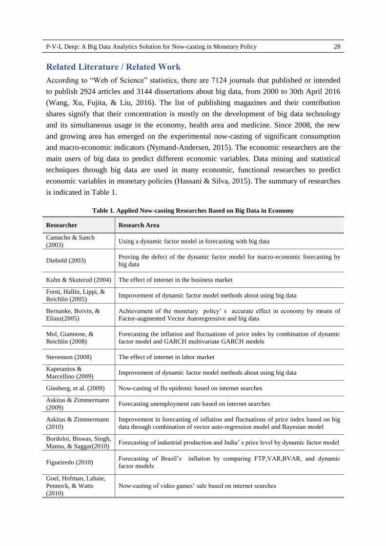
Related Literature / Related Work
According to “Web of Science” statistics, there are 7124 journals that published or intended
to publish 2924 articles and 3144 dissertations about big data, from 2000 to 30th April 2016
(Wang, Xu, Fujita, & Liu, 2016). The list of publishing magazines and their contribution
shares signify that their concentration is mostly on the development of big data technology
and its simultaneous usage in the economy, health area and medicine. Since 2008, the new
and growing area has emerged on the experimental now-casting of significant consumption
and macro-economic indicators (Nymand-Andersen, 2015). The economic researchers are the
main users of big data to predict different economic variables. Data mining and statistical
techniques through big data are used in many economic, functional researches to predict
economic variables in monetary policies (Hassani & Silva, 2015). The summary of researches
is indicated in Table 1.
Table 1. Applied Now-casting Researches Based on Big Data in Economy
Researcher Research Area
Camacho & Sanch
(2003) Using a dynamic factor model in forecasting with big data
Diebold (2003) Proving the defect of the dynamic factor model for macro-economic forecasting by
big data
Kuhn & Skuterud (2004) The effect of internet in the business market
Forni, Hallin, Lippi, &
Reichlin (2005) Improvement of dynamic factor model methods about using big data
Bernanke, Boivin, &
Eliasz(2005)
Achievement of the monetary policy’ s accurate effect in economy by means of
Factor-augmented Vector Autoregressive and big data
Mol, Giannone, &
Reichlin (2008)
Forecasting the inflation and fluctuations of price index by combination of dynamic
factor model and GARCH multivariate GARCH models
Stevenson (2008) The effect of internet in labor market
Kapetanios &
Marcellino (2009) Improvement of dynamic factor model methods about using big data
Ginsberg, et al. (2009) Now-casting of flu epidemic based on internet searches
Askitas & Zimmermann
(2009) Forecasting unemployment rate based on internet searches
Askitas & Zimmermann
(2010)
Improvement in forecasting of inflation and fluctuations of price index based on big
data through combination of vector auto-regression model and Bayesian model
Bordoloi, Biswas, Singh,
Manna, & Saggar(2010) Forecasting of industrial production and India’ s price level by dynamic factor model
Figueiredo (2010) Forecasting of Brazil’s inflation by comparing FTP,VAR,BVAR, and dynamic
factor models
Goel, Hofman, Lahaie,
Pennock, & Watts
(2010)
Now-casting of video games’ sale based on internet searches

Journal of Information Technology Management, 2020, Vol.12, No.4 29
Researcher Research Area
Carriero, Kapetanios, &
Marcellino (2011)
Forecasting of industrial production indicators, consumer price and federal funds’
rate by multivariate Bayesian model, through time series’ big data of 52 macro-
economic indicators derived from Stock and Watson data(2006)
Carriero, Clark, &
Marcellino (2012a)
Now-casting with big data through combination of Bayesian Mixed frequency model
with probable fluctuations for real-time forecasting of America’s GDP
Carriero, Kapetanios, &
Marcellino (2012b)
Forecasting of interest rate by big scale BVAR model with optimized contraction
towards auto-regression model
Giovanelli (2012)
Forecasting industrial production indicators and consumer price by PCA and
artificial neural net including 259 forecasters for Euro and 131 forecasters for
America’s economy
Doz, Giannone, &
Reichlin (2012)
Evaluation of factor model’s maximum likelihood estimation (MLE) for big data
forecasting through simulation
Choi & Varian (2012) Forecasting of economic indicators based on Google search engine’s data by a
seasonal auto-regression model based on big data
Choi & Varian (2012) Forecasting of unemployment rate based on internet searches
Gupta, Kabundi, Miller,
& Uwilingiye (2013)
Forecasting of employment in 8 America’s economic sectors by added agent
Bayesian multi-variable multivariate factor-augmented Bayesian shrinkage model
based on big data
Banerjee, Marcellino, &
Masten (2013)
Forecasting the rate of Euro, Pond and Japan’s Factor-augmented Error Correction
Model based on big data
Banerjee, Marcellino, &
Masten(2013)
Forecasting of America’s and Germany’s inflation and interest rates by FECM
model based on big data
Ouysse(2013) Forecasting of America’s inflation and industrial production by the average of
Bayesian Model Averaging and Principal Component Regression based on big data
Koop(2013) Now-casting of GDP growth by BVAR models based on big data
Lahiri & Monokroussos
(2013)
Investigating consumer’s coefficient of confidence in personal consumption
expenses by dynamic factor model based on real-time big data
Soto, Frias-Martinez,
Virseda, & Frias-
Martinez (2011)
Classification of an area’s social-economic level by support vector machine model,
random forest and regression
Bańbura, Giannone, &
Lenza (2014 & 2015)
Forecasting of 26 economic and financial macro-indicators of Euro zone and
analysis of scenario by the suggested algorithm based on Kalman filtering for VAR’
and DFM’s large models
Bańbura & Modugno
(2014) Using factor models with maximum likelihood estimation based on 101 time-series
Kroft & Pope(2014) The effect of internet in business market
Tuhkuri (2014) Now-casting of unemployment rate based on internet searches

P-V-L Deep: A Big Data Analytics Solution for Now-casting in Monetary Policy 30
Researcher Research Area
Kuhn & Mansour (2014) The effect of internet in business market
Wu & Brynjolfsson
(2015) Now-casting of housing market deals based on internet searches
Lahiri & Monokroussos
(2015)
Improvement of now-casting trend by investigating the survey effect in America’s
GDP growth
Galbraith & Tkacz
(2016)
Improvement of now-casting performance in GDP growth and retail based on
payment data
Tuhkuri (2016) Forecasting of Finland’s economic unemployment rate’s indicator based on big data
by vector autoregressive seasonally adjusted time-series model
Li (2016) Now-casting of unemployed and employed people’s initial requests by factor model
Alvarez & Perez-Quiros
(2016)
Investigating dynamic factor model based on big data in forecasting of economic
macro-indicators
Tiffin (2016)
Offering the now-casting of GDP based on real-time data by machine learning
model, based on “out-of-sample” approach, considering simulation techniques of
autonomous style and using two approaches of Elastic Net Regression and deciding
tree to select variables and reduce dimensions
Hindrayanto,
JanKoopman, & Winter
(2016)
Evaluation of 4 factor models’ performances in pseudo real-time for Euro and 5 big
countries
Bragolia & Modugno
(2016)
Offering an economic model for real forecasting (now-casting) of Canada’s GDP
indicator based on dynamic factor model by combination of on-time, high-frequency
data
Chernis & Sekkel (2017) Forecasting of Canada’s economic indicators based on big data
Bragolia & Modugno
(2017)
Now-casting of Japan’s macro-economic by combination of on-time, high-frequency
data
Federal Reserved Bank
(2017)
Now-casting of GDP based on big data by Kalman filtering method and dynamic
factor model
Duarte, Rodrigues, &
Rua (2017)
Forecasting of private consumptions by using high-frequency data and records of
POSs and ATMs by MIDAS
Njuguna (2017) Investigation of correlation rate between the night light proxy index and economic
activity by Graphically weighted regression
Lu (2019)
Offering a monetary policy prediction model based on deep learning by using the
timing weights back propagation model to analyzes 28 interest rate changes of
China’s macro-monetary policy and the mutual influences between reserve
adjustments and financial markets for time-series according to the data correlation
between financial market and monetary policy
Ostapenko (2020) Identifying exogenous monetary policy shocks with deep learning and basic machine
learning regressors (SVAR)
Yasir, et al. (2020) Designing an efficient algorithm for interest rate prediction using twitter sentiment
analysis
Journal of Information Technology Management, 2020, Vol.12, No.4 31
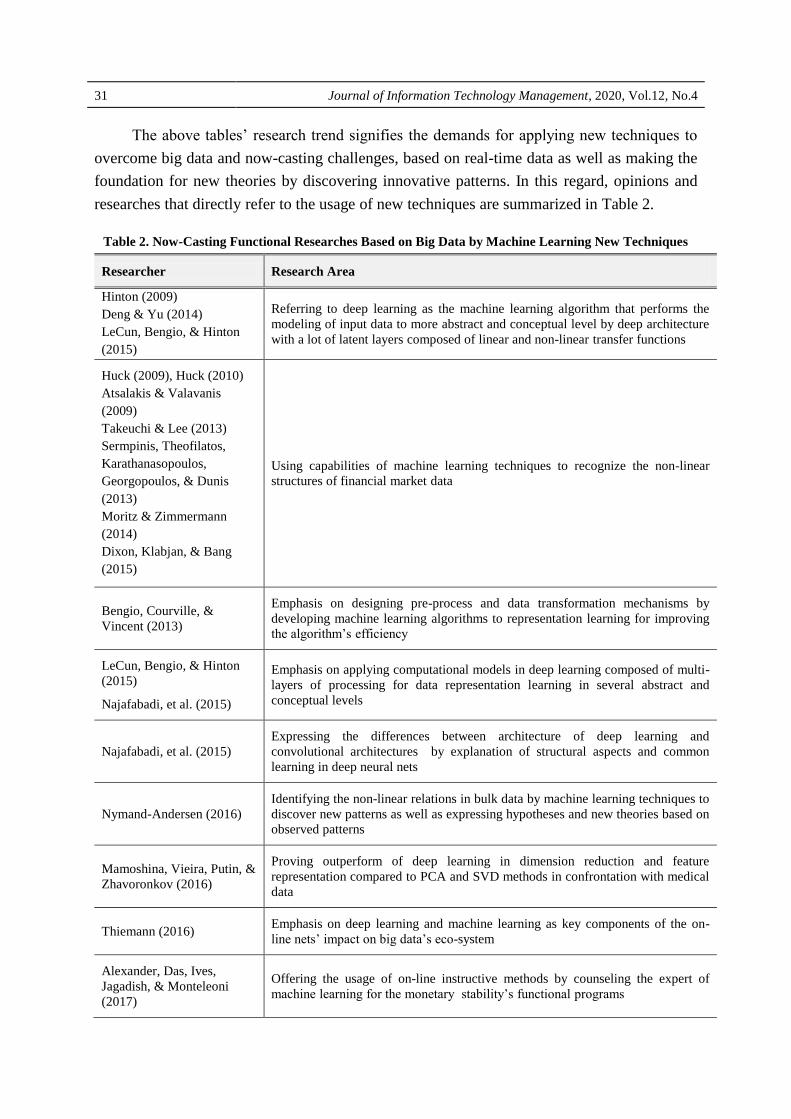
The above tables’ research trend signifies the demands for applying new techniques to
overcome big data and now-casting challenges, based on real-time data as well as making the
foundation for new theories by discovering innovative patterns. In this regard, opinions and
researches that directly refer to the usage of new techniques are summarized in Table 2.
Table 2. Now-Casting Functional Researches Based on Big Data by Machine Learning New Techniques
Researcher Research Area
Hinton (2009)
Deng & Yu (2014)
LeCun, Bengio, & Hinton
(2015)
Referring to deep learning as the machine learning algorithm that performs the
modeling of input data to more abstract and conceptual level by deep architecture
with a lot of latent layers composed of linear and non-linear transfer functions
Huck (2009), Huck (2010)
Atsalakis & Valavanis
(2009)
Takeuchi & Lee (2013)
Sermpinis, Theofilatos,
Karathanasopoulos,
Georgopoulos, & Dunis
(2013)
Moritz & Zimmermann
(2014)
Dixon, Klabjan, & Bang
(2015)
Using capabilities of machine learning techniques to recognize the non-linear
structures of financial market data
Bengio, Courville, &
Vincent (2013)
Emphasis on designing pre-process and data transformation mechanisms by
developing machine learning algorithms to representation learning for improving
the algorithm’s efficiency
LeCun, Bengio, & Hinton
(2015)
Najafabadi, et al. (2015)
Emphasis on applying computational models in deep learning composed of multi-
layers of processing for data representation learning in several abstract and
conceptual levels
Najafabadi, et al. (2015)
Expressing the differences between architecture of deep learning and
convolutional architectures by explanation of structural aspects and common
learning in deep neural nets
Nymand-Andersen (2016)
Identifying the non-linear relations in bulk data by machine learning techniques to
discover new patterns as well as expressing hypotheses and new theories based on
observed patterns
Mamoshina, Vieira, Putin, &
Zhavoronkov (2016)
Proving outperform of deep learning in dimension reduction and feature
representation compared to PCA and SVD methods in confrontation with medical
data
Thiemann (2016) Emphasis on deep learning and machine learning as key components of the on-
line nets’ impact on big data’s eco-system
Alexander, Das, Ives,
Jagadish, & Monteleoni
(2017)
Offering the usage of on-line instructive methods by counseling the expert of
machine learning for the monetary stability’s functional programs
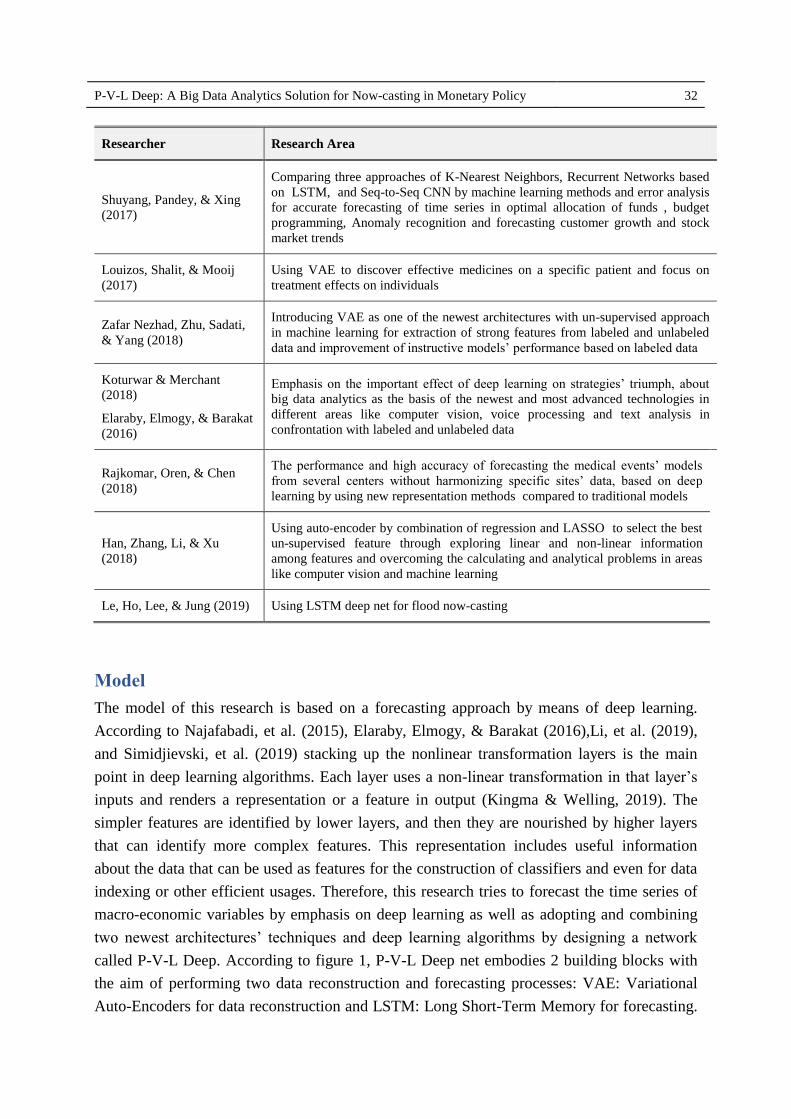
P-V-L Deep: A Big Data Analytics Solution for Now-casting in Monetary Policy 32
Researcher Research Area
Shuyang, Pandey, & Xing
(2017)
Comparing three approaches of K-Nearest Neighbors, Recurrent Networks based
on LSTM, and Seq-to-Seq CNN by machine learning methods and error analysis
for accurate forecasting of time series in optimal allocation of funds , budget
programming, Anomaly recognition and forecasting customer growth and stock
market trends
Louizos, Shalit, & Mooij
(2017)
Using VAE to discover effective medicines on a specific patient and focus on
treatment effects on individuals
Zafar Nezhad, Zhu, Sadati,
& Yang (2018)
Introducing VAE as one of the newest architectures with un-supervised approach
in machine learning for extraction of strong features from labeled and unlabeled
data and improvement of instructive models’ performance based on labeled data
Koturwar & Merchant
(2018)
Elaraby, Elmogy, & Barakat
(2016)
Emphasis on the important effect of deep learning on strategies’ triumph, about
big data analytics as the basis of the newest and most advanced technologies in
different areas like computer vision, voice processing and text analysis in
confrontation with labeled and unlabeled data
Rajkomar, Oren, & Chen
(2018)
The performance and high accuracy of forecasting the medical events’ models
from several centers without harmonizing specific sites’ data, based on deep
learning by using new representation methods compared to traditional models
Han, Zhang, Li, & Xu
(2018)
Using auto-encoder by combination of regression and LASSO to select the best
un-supervised feature through exploring linear and non-linear information
among features and overcoming the calculating and analytical problems in areas
like computer vision and machine learning
Le, Ho, Lee, & Jung (2019) Using LSTM deep net for flood now-casting
Model
The model of this research is based on a forecasting approach by means of deep learning.
According to Najafabadi, et al. (2015), Elaraby, Elmogy, & Barakat (2016),Li, et al. (2019),
and Simidjievski, et al. (2019) stacking up the nonlinear transformation layers is the main
point in deep learning algorithms. Each layer uses a non-linear transformation in that layer’s
inputs and renders a representation or a feature in output (Kingma & Welling, 2019). The
simpler features are identified by lower layers, and then they are nourished by higher layers
that can identify more complex features. This representation includes useful information
about the data that can be used as features for the construction of classifiers and even for data
indexing or other efficient usages. Therefore, this research tries to forecast the time series of
macro-economic variables by emphasis on deep learning as well as adopting and combining
two newest architectures’ techniques and deep learning algorithms by designing a network
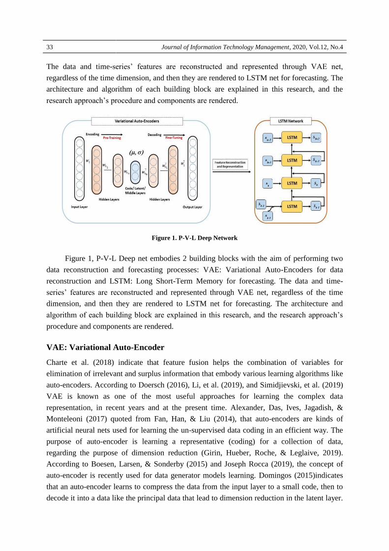
called P-V-L Deep. According to figure 1, P-V-L Deep net embodies 2 building blocks with
the aim of performing two data reconstruction and forecasting processes: VAE: Variational
Auto-Encoders for data reconstruction and LSTM: Long Short-Term Memory for forecasting.
Journal of Information Technology Management, 2020, Vol.12, No.4 33
The data and time-series’ features are reconstructed and represented through VAE net,
regardless of the time dimension, and then they are rendered to LSTM net for forecasting. The
architecture and algorithm of each building block are explained in this research, and the
research approach’s procedure and components are rendered.
Figure 1. P-V-L Deep Network
Figure 1, P-V-L Deep net embodies 2 building blocks with the aim of performing two
data reconstruction and forecasting processes: VAE: Variational Auto-Encoders for data
reconstruction and LSTM: Long Short-Term Memory for forecasting. The data and time-
series’ features are reconstructed and represented through VAE net, regardless of the time
dimension, and then they are rendered to LSTM net for forecasting. The architecture and
algorithm of each building block are explained in this research, and the research approach’s
procedure and components are rendered.
VAE: Variational Auto-Encoder
Charte et al. (2018) indicate that feature fusion helps the combination of variables for
elimination of irrelevant and surplus information that embody various learning algorithms like
auto-encoders. According to Doersch (2016), Li, et al. (2019), and Simidjievski, et al. (2019)
VAE is known as one of the most useful approaches for learning the complex data
representation, in recent years and at the present time. Alexander, Das, Ives, Jagadish, &
Monteleoni (2017) quoted from Fan, Han, & Liu (2014), that auto-encoders are kinds of
artificial neural nets used for learning the un-supervised data coding in an efficient way. The
purpose of auto-encoder is learning a representative (coding) for a collection of data,
regarding the purpose of dimension reduction (Girin, Hueber, Roche, & Leglaive, 2019).
According to Boesen, Larsen, & Sonderby (2015) and Joseph Rocca (2019), the concept of
auto-encoder is recently used for data generator models learning. Domingos (2015)indicates
that an auto-encoder learns to compress the data from the input layer to a small code, then to
decode it into a data like the principal data that lead to dimension reduction in the latent layer.

P-V-L Deep: A Big Data Analytics Solution for Now-casting in Monetary Policy 34
Bengio (2009), from an architectural point of view, defines the simplest form of auto-
encoders as a feed-forward, non-recurrent net, that is greatly like a single perceptron layer to
make the multi-layer perceptron. This architecture is composed of an input, an output and
several latent layers in which the number of knots in the output layer is equal with the input
layer with the purpose of input reconstruction (instead of forecasting the amount of Y target
based on inputs of X vector). In this way, auto-encoders are un-supervised learning models.
The same as Suk, Lee, & Shen (2016), defines auto-encoder as an artificial neural net that is
structurally made of three layers: input, latent, and output in which the input layer in
completely connected to the latent layer and the latent layer is completely connected to the
output layer. The purpose of auto-encoders is learning a compressed representation or a latent
one from input through minimizing the reconstruction errors between input and represented
date. According to Dai, Tian, Dai, Skiena, & Song (2018), adopting generative models with
discrete structured data is very popular among researchers, while its usage is growing in
various areas. According to Galeshchuk & Mukherjee (2017), quoted from Lee, Ekanadham,
& Ng (2008) and Vincent et al. (2010), the number of input and output units conforms to the
dimensions of input vector, while the number of the latent layer’s units can be determined
based on the data’s nature. If the number of latent layers is lower than the input layers, the
auto-encoder is used to reduce the dimensions. However, for achievement of complex and
non-linear relations among features, we can consider the number of the latent layers more
than input layers orwe can gain an attractive structure by applying sparsity limit. In this
regard, Vincent et al. (2010) indicate that the choice of deep architecture can intensely affect
the feature representation, since the number of latent layers can be more or less than principal
features. According to Charte et al. (2018) and, the researchers mostly try to reduce the data
dimensions (Under-Complete Representation) and to represent data with more dimensions
(Over-complete Representation) as a substitution for Under-Complete representation.
Figure 2. Types of Deep Architecture
According to figure 2, the auto-encoder achieves this purpose by combining the
principal features based on the determined weights through learning procedure, in the Under-
Complete architecture. In Over-Complete architecture; the auto-encoder applies the identical
function learning based on duplication of input in output.

Journal of Information Technology Management, 2020, Vol.12, No.4 35
VAE Network’s Algorithm and Performance
According to Charte et al. (2018), the purpose of VAE is the distribution of latent variables
based on observations.VAE substitutes the definite functions in encoding and decoding using
random mapping and calculation of target function for density functions of random variables.
In other words, according to Joseph Rocca (2019)and Dai et al. (2018)quoted from Diederik
& Welling (2013), Zafar Nezhad, Zhu, Sadati, & Yang (2018), Liangchen & Deng (2017),
Rezende, Mohamed, & Wierstra (2014), VAE is a generative model of a standard auto-
encoders’ reformed version that has a learnable prior recognition model, in its architecture
rather than the definite function of standard auto-encoders architecture. Figure 3 signifies that
encoding space is a probability space and if owning Z, the decoding space renders
reconstructed will X as output.
Figure 3. Algorithm of Variational Auto-encoder
According to figure 4, and based on Simidjievski, et al. (2019), Kingma & Welling
(2019), Li, et al. (2019), (Girin, Hueber, Roche, & Leglaive (2019), and Zafar Nezhad M.,
Zhu, Sadati, & Yang (2018), VAE has three layers of encoding, decoding and latent, as a
probabilistic generative model.
Figure 4. A Schema of Variational Auto-encoder
P-V-L Deep: A Big Data Analytics Solution for Now-casting in Monetary Policy 36
If X is assumed as the input data and Z as the latent variable, based on the total
probability law, VAE tries to maximize the probability of each X in the training set by the
following equations in a generative procedure based on Total probability law:
𝑃 𝑥 = 𝑃 𝑋, 𝑧 𝑑𝑧 = 𝑃 𝑋 𝑧 𝑃 𝑧 𝑑𝑧 (1)
According to Diederik & Welling (2013), this model inherits the architecture of auto-
encoder but renders strong hypotheses about the distribution of latent variables.
It uses a variational approach for latent representation learning that leads to another
Loss component and a specific learning algorithm called SGVB1.
According to Charte et al. (2018), it is assumed that an unsupervised, unknown random
variable leads to X observations through a stochastic process.
Zafar Nezhad M., Zhu, Sadati, & Yang (2018), Liangchen & Deng (2017), Partaourides
& Chatzis (2017) indicate that data is assumingly produced by directed graphical model
𝑝 𝑥 𝑧 in VAE’s algorithm, then the encoder learns the approximation of 𝑞ȹ 𝑧 𝑥 to the
posterior distribution of 𝑝𝜃 𝑧 𝑥 ; While ȹ and θ signify parameters of encoder
(discriminative model or inference model) and decoder (generative model). The objective
functionis as following:
ℒ ȹ,𝜃, 𝑥 = 𝐷𝐾𝐿(𝑞𝜑 𝑧 𝑥 𝑝𝜃(𝑧)) − 𝔼𝑞ȹ 𝑧 𝑥 𝑙𝑜𝑔 𝑝𝜃 𝑥 𝑧 (2)
According to Hsu & Kira (2016), DKL under the title of divergence of KL:
Kullback_Leibler,is conventionally used for estimation of measuring the distance between
output distribution and the main ground truth distribution. In other words, in mathematical
statistics, there is a criterion to show how one probability distribution diverges from a second,
reference probability distribution.KL divergence of 0 shows that similarity can be expected,
otherwise different behaviors of two distributions are expected, while the first distribution is
expected to approach zero. In a simple word, KL has an interesting criterion with various
functions (diverse applications) in applied statistics, fluid mechanics, neuro-science and
machine learning.
The prior over the latent variables is usually arranged to multi-variant Gaussian that
converged to the center.
𝑝𝜃 𝑧 = 𝑁(0, 𝐼) (3)
ـــــــــــــــــــــــــــــــــــــــــــــــــــــــــــــــــــــــــــــــــــــــــــــــــــــــــــــــــــــــــــــــــــــــــــــــــــــــــــــــــــــــــــــــــــــــــــــــــــــــ1. Stochastic Gradient Variational Bayes
Journal of Information Technology Management, 2020, Vol.12, No.4 37
Zafar Nezhad M., Zhu, Sadati, & Yang (2018) indicate that the structure of auto-
encoders is formed based on Bayesian rule by considering q as the encoder of x to z and p as
its decoder to reconstruct x.
Weighting VAE Net
According to Mendels (2019) and Koturwar & Merchant (2018; 2019), in spite of the very
strong performance of deep nets and advances of computational technologies, it seems that
few researchers try to train their nets from the beginning. The researcher’s main challenge
during training the net is the vanishing / exploding gradient problems as well as handling the
non-convex essence of target function that has over one million variables. The recommended
approaches by Xavier (2010) and He (2015) are rendering a proper initial weighing method to
solve the problem of vanishing gradient. These approaches have had very great impacts on
standard databases. While based on Saiprasad Koturwar’s research (2018; 2019), the
recommended approaches of Xavier (2010) and He (2015) did not have proper effects on
more practical databases, due to absence of statistical data for initializing the net’s weights.
The method of Xavier is independent of data statistics while depending only on the
net’s size. However, optimizing the loss function (cost function) with high dimensions needs
the accurate initializing of the net’s weights; since it will have millions of variables by
increasing the size of the net even to 3 or 4 layers. Therefore, finding a proper initializing is
very important to gain better results.
Koturwar & Merchant (2018) and (2019) recommends and analyzes a new method for
data-dependent initializing and compares the model to the standard method of He and Xavier
to gain better results about some practical databases as well as achieving the algorithm’s
classification accuracy.
Weight calculation according to He and Xavier standard is as following in domain of
low (-) and high (+):
𝑤 = 6
𝑛𝑖𝑛𝑝𝑢𝑡𝑠 + 𝑛𝑜𝑢𝑡𝑝𝑢𝑡𝑠
2
(4)
LSTM: Long Short-Term Memory Nets
LSTM net was introduced by Hochreiter & Schmidhuber (1997)and was named by Gers,
Schmidhuber, & Cummins (2000), Graves & Schmidhuber (2005) and Graves et al. (2009). It
was rendered as a category of recurrent neural nets by Medsker (2000). Then separate
researches were done by means of LSTM by Graves et al. (2009; 2013), and Schmidhuber
(2015). According to Sak, Senior, & Beaufays (2014) and Wong, Shi, Yeung, & Woo (2016),
P-V-L Deep: A Big Data Analytics Solution for Now-casting in Monetary Policy 38
these nets are specifically designed for long-term dependence’s learning as well as having the
ability to overcome recurrent neural nets’ innate problems, including vanishing gradient
problem. Furthermore, LSTM nets were described by Graves (2014), Olah (2015)and Chollet
(2016)and valuable introduction was presented by Staudemeyer & Morris (2019), Karpathy
(2015), and Britz (2015).
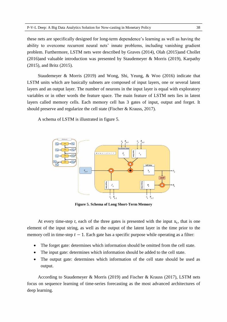
Staudemeyer & Morris (2019) and Wong, Shi, Yeung, & Woo (2016) indicate that
LSTM units which are basically subnets are composed of input layers, one or several latent
layers and an output layer. The number of neurons in the input layer is equal with exploratory
variables or in other words the feature space. The main feature of LSTM nets lies in latent
layers called memory cells. Each memory cell has 3 gates of input, output and forget. It
should preserve and regularize the cell state (Fischer & Krauss, 2017).
A schema of LSTM is illustrated in figure 5.
Figure 5. Schema of Long Short-Term Memory
At every time-step t, each of the three gates is presented with the input xt , that is one
element of the input string, as well as the output of the latent layer in the time prior to the
memory cell in time-step 𝑡 − 1. Each gate has a specific purpose while operating as a filter:
The forget gate: determines which information should be omitted from the cell state.
The input gate: determines which information should be added to the cell state.
The output gate: determines which information of the cell state should be used as
output.
According to Staudemeyer & Morris (2019) and Fischer & Krauss (2017), LSTM nets
focus on sequence learning of time-series forecasting as the most advanced architectures of
deep learning.

Journal of Information Technology Management, 2020, Vol.12, No.4 39
The results of his research in adopting LSTM nets indicate that these nets operated
better than memory-free classification` methods like random forest, deep neural nets and
logistic regression classifiers for out of sample forecasting of 500 S & P data, from 1992 to
2015. The findings comparison of Krauss, Do, & Huck (2017) recent research on survey data
of over 100 investment market anomalies through deep learning, random forest, reinforced
gradient tree and other forecasting methods signify the deep neural nets’ great progress in
time-series forecasting.
LSTM Net’s Algorithm and Performance
This net’s performance in the cell states st and the latent layer’s outputs in 𝑡 are calculated as
following in LSTM layer in each time step of 𝑡:
1. Calculation of activation function of 𝑓𝑡 to determine the previous state cell’s information
𝑠𝑡−1 based on input of 𝑥𝑡 and output of 𝑡−1from memory cells in time step of 𝑡 − 1 and
bias values of 𝑏𝑓 :
𝑓𝑡 = 𝑠𝑖𝑔𝑚𝑜𝑖𝑑 𝑤𝑓 ,𝑥𝑥𝑡 + 𝑤𝑓 ,𝑡−1 + 𝑏𝑓 (5)
Sigmoid function scales all activation values between zero (complete dropout) and one
(complete saving).
2. Determination of required information to be added to the cell state (𝑠𝑡) by calculation of
𝑠 𝑡and 𝑖𝑡 :
𝑠 𝑡= 𝑡𝑎𝑛(𝑤𝑠 ,𝑥𝑥𝑡 + 𝑤𝑠 ,𝑡−1+𝑏𝑠 ) (6)
𝑖𝑡 = 𝑠𝑖𝑔𝑚𝑜𝑖𝑑(𝑤𝑖,𝑥𝑥𝑡 + 𝑤𝑖,𝑡−1+𝑏𝑖) (7)
3. Calculation of the new cell state according to the results of the previous two steps with ◦
denoting the Hadamard product:
𝑠𝑡 = 𝑓𝑡 ° 𝑠𝑡−1 + 𝑖𝑡°𝑠 𝑡 (8)
4. Calculating 𝑜𝑡 and 𝑡 :
𝑜𝑡 = 𝑠𝑖𝑔𝑚𝑜𝑖𝑑(𝑤𝑜,𝑥𝑥𝑡 + 𝑤𝑜 ,𝑡−1+𝑏𝑜) (9)
𝑡 = 𝑜𝑡 ° 𝑡𝑎𝑛( 𝑠𝑡) (10)
P-V-L Deep: A Big Data Analytics Solution for Now-casting in Monetary Policy 40
Methodology of the Research
Data, Software, and Hardware Used in Research
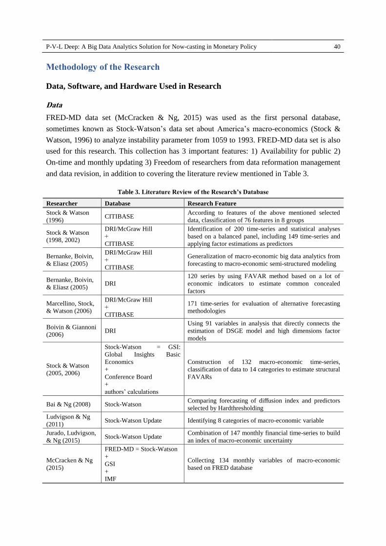
Data
FRED-MD data set (McCracken & Ng, 2015) was used as the first personal database,
sometimes known as Stock-Watson’s data set about America’s macro-economics (Stock &
Watson, 1996) to analyze instability parameter from 1059 to 1993. FRED-MD data set is also
used for this research. This collection has 3 important features: 1) Availability for public 2)
On-time and monthly updating 3) Freedom of researchers from data reformation management
and data revision, in addition to covering the literature review mentioned in Table 3.
Table 3. Literature Review of the Research’s Database
Researcher Database Research Feature
Stock & Watson
(1996) CITIBASE
According to features of the above mentioned selected
data, classification of 76 features in 8 groups
Stock & Watson
(1998, 2002)
DRI/McGraw Hill
+
CITIBASE
Identification of 200 time-series and statistical analyses
based on a balanced panel, including 149 time-series and
applying factor estimations as predictors
Bernanke, Boivin,
& Eliasz (2005)
DRI/McGraw Hill
+
CITIBASE
Generalization of macro-economic big data analytics from
forecasting to macro-economic semi-structured modeling
Bernanke, Boivin,
& Eliasz (2005) DRI
120 series by using FAVAR method based on a lot of
economic indicators to estimate common concealed
factors
Marcellino, Stock,
& Watson (2006)
DRI/McGraw Hill
+
CITIBASE
171 time-series for evaluation of alternative forecasting
methodologies
Boivin & Giannoni
(2006) DRI
Using 91 variables in analysis that directly connects the
estimation of DSGE model and high dimensions factor
models
Stock & Watson
(2005, 2006)
Stock-Watson = GSI:
Global Insights Basic
Economics
+
Conference Board
+
authors’ calculations
Construction of 132 macro-economic time-series,
classification of data to 14 categories to estimate structural
FAVARs
Bai & Ng (2008) Stock-Watson Comparing forecasting of diffusion index and predictors
selected by Hardthresholding
Ludvigson & Ng
(2011) Stock-Watson Update Identifying 8 categories of macro-economic variable
Jurado, Ludvigson,
& Ng (2015) Stock-Watson Update
Combination of 147 monthly financial time-series to build
an index of macro-economic uncertainty
McCracken & Ng
(2015)
FRED-MD = Stock-Watson
+
GSI
+
IMF
Collecting 134 monthly variables of macro-economic
based on FRED database
Journal of Information Technology Management, 2020, Vol.12, No.4 41
Therefore, data was used as out of sample forecasting, in this research and CSV files
and other explanations or researches related to this database are available in the address of
http://research.stlouisfed.org/econ/mccracken/sel/.This file is composed of current and
historical data. Due to some reasons, it is not a balanced panel, although, it can easily
transform into a balanced panel by the elimination of interrelated relevant series. Based on
economic elites’ opinions, the data average of each feature’s column was used in missing
columns for transforming into a balanced panel in the data pre-processing stage.
Software and Hardware
For data pre-processing from python 3.5, steps mentioned in section Approach were
performed on the basis of numpy, panda, tkinter, sklearn and sklearn preprocessing packages.
Deep learning of VAE and LSTM is developed by means of Keras library in Tensor flow. It is
a very strong library for large scale machine learning of heterogeneous systems.
The designed net model was trained on the laptop of NVIDIA GTX 1060 GPU Support,
Intel Core i7.
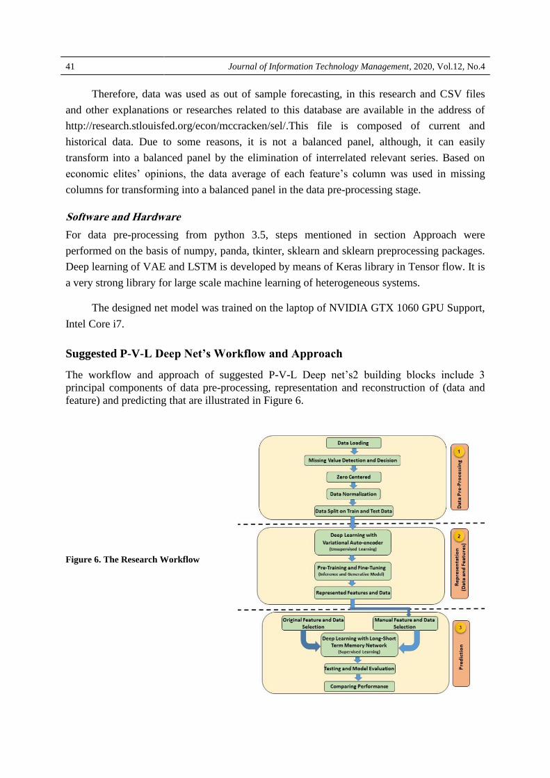
Suggested P-V-L Deep Net’s Workflow and Approach
The workflow and approach of suggested P-V-L Deep net’s2 building blocks include 3
principal components of data pre-processing, representation and reconstruction of (data and
feature) and predicting that are illustrated in Figure 6.
Figure 6. The Research Workflow

P-V-L Deep: A Big Data Analytics Solution for Now-casting in Monetary Policy 42
As it is obvious in figure 6 each component of workflow and approach include the
following steps:
Steps of component 1: Data Pre-Processing
Data uploading
Recognizing and deciding in confrontation with missing values
Zero centered
Normalizing data
Separation of raw data to collections of train and test data
Steps of component 2: Representation and Reconstruction (data and feature)
Unsupervised deep learning by using VAE net
Pre-training, fine-tuning, and improvement of feature through discriminative /
inference model and generative model
Representation of features and reconstruction of data
Deciding about features space and target variables for training and predicting
Steps of component 3: Prediction
Manual selection of a feature from represented and reconstructed features through
VAE net
Selection of the same feature and data from the original and raw data file
Supervised deep learning by LSTM nets special for time-series forecasting
Training, testing and evaluating and validation the model based on raw and
reconstructed data
Comparing the predicting performance
Steps of Component 1: Data Pre-Processing
The CSV file that is composed of 720 observations (lines) and 129 features (columns) was
uploaded along with the Header. The amounts of NaN in the columns were identified by
represented statistical information through the program, and then they were substituted by
each column’s average. After, zero-centered stages and data normalization were performed
for comparison through 2 methods:
The first method is applying the averaging and the standard deviation by means of
each column’s mean and std. functions.
The second method is applying the Standard Scaler function from sklearn. pre-
processing package.
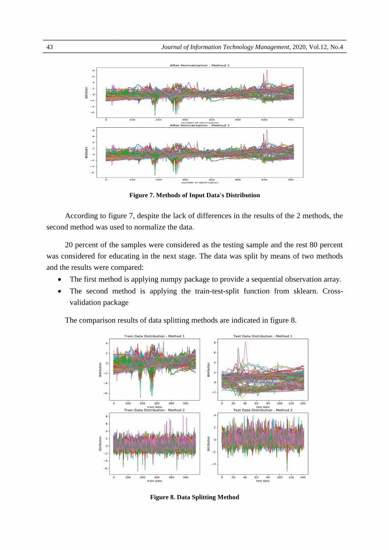
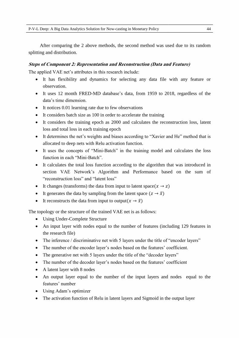
The comparison results of the input data’s distribution are indicated in figure 7 the
results show that the performance of the two methods is exactly the same.
Journal of Information Technology Management, 2020, Vol.12, No.4 43
Figure 7. Methods of Input Data's Distribution
According to figure 7, despite the lack of differences in the results of the 2 methods, the
second method was used to normalize the data.
20 percent of the samples were considered as the testing sample and the rest 80 percent
was considered for educating in the next stage. The data was split by means of two methods
and the results were compared:
The first method is applying numpy package to provide a sequential observation array.
The second method is applying the train-test-split function from sklearn. Cross-
validation package
The comparison results of data splitting methods are indicated in figure 8.
Figure 8. Data Splitting Method
P-V-L Deep: A Big Data Analytics Solution for Now-casting in Monetary Policy 44
After comparing the 2 above methods, the second method was used due to its random
splitting and distribution.
Steps of Component 2: Representation and Reconstruction (Data and Feature)
The applied VAE net’s attributes in this research include:
It has flexibility and dynamics for selecting any data file with any feature or
observation.
It uses 12 month FRED-MD database’s data, from 1959 to 2018, regardless of the
data’s time dimension.
It notices 0.01 learning rate due to few observations
It considers batch size as 100 in order to accelerate the training
It considers the training epoch as 2000 and calculates the reconstruction loss, latent
loss and total loss in each training epoch
It determines the net’s weights and biases according to “Xavier and He” method that is
allocated to deep nets with Relu activation function.
It uses the concepts of “Mini-Batch” in the training model and calculates the loss
function in each “Mini-Batch”.
It calculates the total loss function according to the algorithm that was introduced in
section VAE Network’s Algorithm and Performance based on the sum of
“reconstruction loss” and “latent loss”
It changes (transforms) the data from input to latent space(𝑥 → 𝑧)
It generates the data by sampling from the latent space (𝑧 → 𝑥 )
It reconstructs the data from input to output(𝑥 → 𝑥 )
The topology or the structure of the trained VAE net is as follows:
Using Under-Complete Structure
An input layer with nodes equal to the number of features (including 129 features in
the research file)
The inference / discriminative net with 5 layers under the title of “encoder layers”
The number of the encoder layer’s nodes based on the features’ coefficient.
The generative net with 5 layers under the title of the “decoder layers”
The number of the decoder layer’s nodes based on the features’ coefficient
A latent layer with 8 nodes
An output layer equal to the number of the input layers and nodes equal to the
features’ number
Using Adam’s optimizer
The activation function of Relu in latent layers and Sigmoid in the output layer

Journal of Information Technology Management, 2020, Vol.12, No.4 45
Steps of Component 3: Prediction
The LSTM net’s features used in this research are as follows:
Using 12-month FRED-MD data from 1959 to 2018, including the principal data and
the data that was reconstructed from VAE net.
Considering 20 percent of samples for the testing sample and the rest 80 percent for
training
Dividing the educational data (80 percent of the principal sample) into 2 training (80
percent) and validation (20 percent) sets. The first sets are applied for the net’s
training as well as its parameters’ moderation and regularization in a repetitive
procedure in order to minimize the loss function. During this procedure, the weights’
and the biases’ amount are moderated and regularized the same as traditional feed-
forward nets in a way that the objective function’s Loss (MSE) reaches its minimum
amount for specified training data
Predicting the un-observed samples from the validation set after each epoch through
the net and calculating the validation loss
Keras applied two advanced methods for LSTM net’s training:
Adopting “RMS-prop” as a version of mini-batch from “rprop” that was introduced by
Tieleman & Hinton (2012) and suggested by Chollet (2016) as a proper choice for
recurrent neural nets and based on Thomas Fischer’s research results (2017) as the
optimizer.
Using the dropout regularization in recurrent layers based on Gal & Ghahramani’s
research (2016). In this method, a part of input units are dropped out randomly in each
updating, during the training time in input gates and recurrent connections. This action
reduces the over-fitting risk and optimizes the generalization.
The topology or the structure of the educated LSTM is as following:
The input layer with one feature and 2000 time steps epoch
The LSTM layer with 128 latent neurons, the dropout amount of 0.2 and the “tanh”
activation function
An output layer with “Sigmoid” activation function
In this stage, it was necessary to provide a feature vector first, then the sequence string
in time-series was designed that leads to producing the output string for the benefit of the
net’s predicting and performance comparison. The predicting was done through the point-by-
point method for each month of the year. Thus, the LSTM net’s input string was produced for
one feature as figure 9 shows.
P-V-L Deep: A Big Data Analytics Solution for Now-casting in Monetary Policy 46
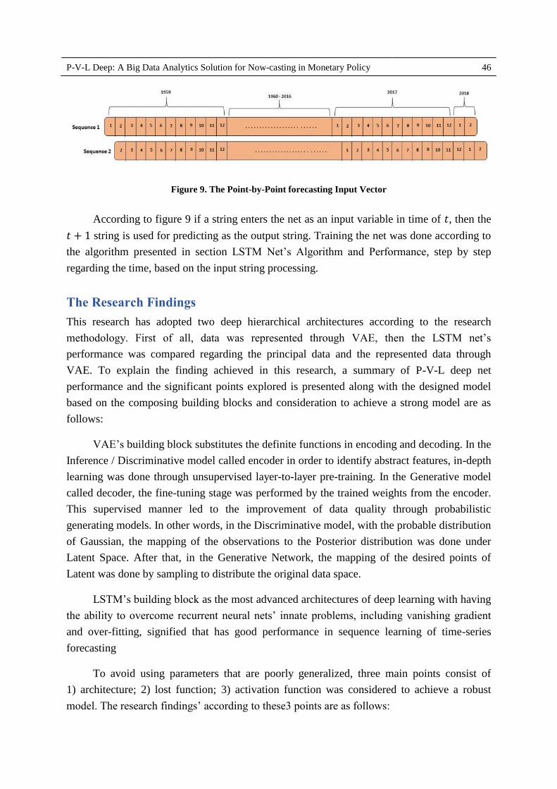
Figure 9. The Point-by-Point forecasting Input Vector
According to figure 9 if a string enters the net as an input variable in time of 𝑡, then the
𝑡 + 1 string is used for predicting as the output string. Training the net was done according to
the algorithm presented in section LSTM Net’s Algorithm and Performance, step by step
regarding the time, based on the input string processing.
The Research Findings
This research has adopted two deep hierarchical architectures according to the research
methodology. First of all, data was represented through VAE, then the LSTM net’s
performance was compared regarding the principal data and the represented data through
VAE. To explain the finding achieved in this research, a summary of P-V-L deep net
performance and the significant points explored is presented along with the designed model
based on the composing building blocks and consideration to achieve a strong model are as
follows:
VAE’s building block substitutes the definite functions in encoding and decoding. In the
Inference / Discriminative model called encoder in order to identify abstract features, in-depth
learning was done through unsupervised layer-to-layer pre-training. In the Generative model
called decoder, the fine-tuning stage was performed by the trained weights from the encoder.
This supervised manner led to the improvement of data quality through probabilistic
generating models. In other words, in the Discriminative model, with the probable distribution
of Gaussian, the mapping of the observations to the Posterior distribution was done under
Latent Space. After that, in the Generative Network, the mapping of the desired points of
Latent was done by sampling to distribute the original data space.
LSTM’s building block as the most advanced architectures of deep learning with having
the ability to overcome recurrent neural nets’ innate problems, including vanishing gradient
and over-fitting, signified that has good performance in sequence learning of time-series
forecasting
To avoid using parameters that are poorly generalized, three main points consist of
1) architecture; 2) lost function; 3) activation function was considered to achieve a robust
model. The research findings’ according to these3 points are as follows:
Journal of Information Technology Management, 2020, Vol.12, No.4 47
VAE deep net:
Considering an under-complete structure and a proper weight initialization approach
to solve the gradient reduction problem that has been completely effective and has had
very good results in the standard database: This weighting method is independent of
data statistics while depending only on the net’s size and was used to prevent the
saturation problem and to neutralize the weights (which makes learning difficult and
especially long in deep nets). In practice, the variance was calibrated according to the
number of inputs and outputs.
Using mini-batch (partial fit) to increase model accuracy, to increase response speed,
to reduce interval covariance shift, and to prevent sparsity: Partial fit applied to all
layers before activation function. In this way, the activation function inputs were
placed in the intermediate range in which the gradient is meaningful.
Using a non-linear activation function to increase the power of the model
Using the regularization term to loss function to prevent exploding / over-fitting,
model sparsity, risk of identity function due to the model's high power, and also avoid
the network out of Deep mode: In fact, it was possible to reconstruct the new data
when the probability of two distributions was as close as possible. Thus, KL as a latent
loss was introduced to loss function. In this research, the model accuracy was
considered the reconstruction loss, and KL loss was considered variational
regularization. So KL was introduced to loss function. Finally, the total loss was
calculated by Latent Loss (KL Divergence) + Reconstruction Loss. In fact, assuming
there is one activation rate for each neuron, the target activation rate was determined.
With this criterion, a distance was determined. Then, with the error rate specified in
the loss function, the rate of activation of the neurons was moved in the opposite
direction to the gradient to reduce the error. Thus, the degree of divergence between
the two probability distributions was measured by KL. Minimizing the KL means
optimizing the probability distribution of the mean parameters and the standard
deviation, this is very similar to the distribution of the objective function. With this
loss, the encoder was encouraged to distribute the data evenly around the latent center.
In each epoch and for each mini-batch, if it moved away from the center, it would be
penalized by clustering in other specific areas. In iterations, feedforward and back-
propagation were performed to produce a result close to the actual output with less
error. Scaling down the error was carried out by Stochastic Gradient Descent (very
similar to multi-layered perspectives). In fact, the parameters were trained to reduce
reconstruction error.
P-V-L Deep: A Big Data Analytics Solution for Now-casting in Monetary Policy 48
LSTM deep net:
Using MSE as a loss function to estimate model accuracy
Using the dropout regularization in recurrent layers during the training time in input
gates and recurrent connections to reduce the over-fitting risk and optimize the
generalization
Applied “RMS-prop” as a version of mini-batch from “rprop” to increase model
accuracy as a proper choice for recurrent neural
VAE net’s Findings
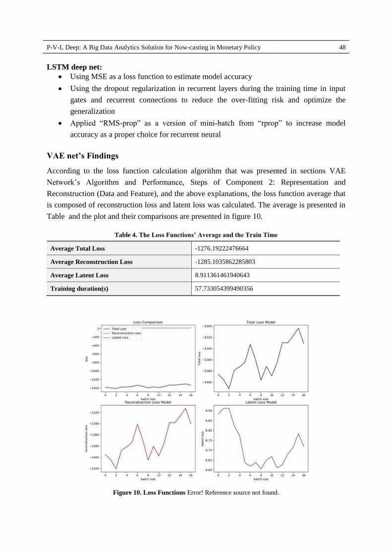
According to the loss function calculation algorithm that was presented in sections VAE
Network’s Algorithm and Performance, Steps of Component 2: Representation and
Reconstruction (Data and Feature), and the above explanations, the loss function average that
is composed of reconstruction loss and latent loss was calculated. The average is presented in
Table and the plot and their comparisons are presented in figure 10.
Table 4. The Loss Functions’ Average and the Train Time
Average Total Loss -1276.19222476664
Average Reconstruction Loss -1285.1035862285803
Average Latent Loss 8.911361461940643
Training duration(s) 57.733054399490356
Figure 10. Loss Functions Error! Reference source not found.
Journal of Information Technology Management, 2020, Vol.12, No.4 49
As it is observed, the loss function in the generative net extremely declines and goes to
zero, compared to the inference / discriminative net. It means that, adopting the weights in
unsupervised learning stage and their corrections, then supervised learning in the generative
net, intensely reduce the loss function and reconstruct the data by corrective weights in order
to gain convergence.
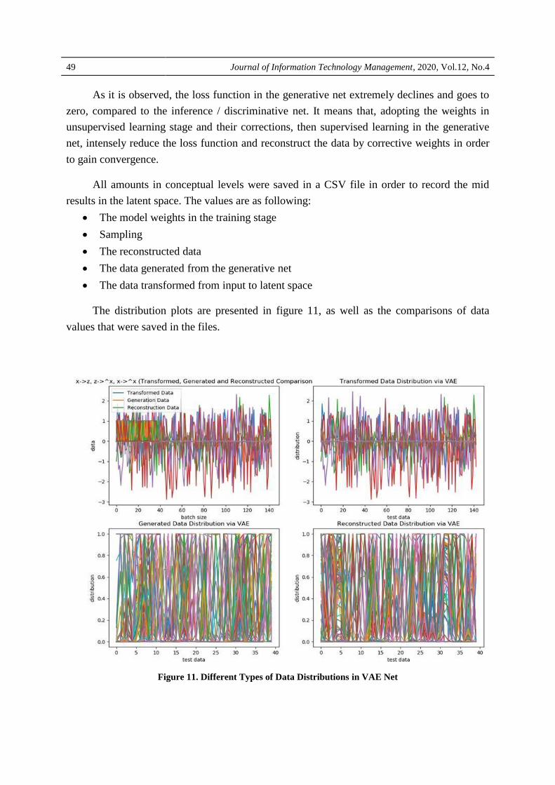
All amounts in conceptual levels were saved in a CSV file in order to record the mid
results in the latent space. The values are as following:
The model weights in the training stage
Sampling
The reconstructed data
The data generated from the generative net
The data transformed from input to latent space
The distribution plots are presented in figure 11, as well as the comparisons of data
values that were saved in the files.
Figure 11. Different Types of Data Distributions in VAE Net
P-V-L Deep: A Big Data Analytics Solution for Now-casting in Monetary Policy 50
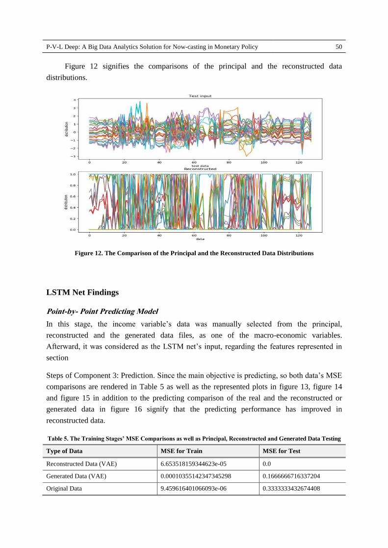
Figure 12 signifies the comparisons of the principal and the reconstructed data
distributions.
Figure 12. The Comparison of the Principal and the Reconstructed Data Distributions
LSTM Net Findings
Point-by- Point Predicting Model
In this stage, the income variable’s data was manually selected from the principal,
reconstructed and the generated data files, as one of the macro-economic variables.
Afterward, it was considered as the LSTM net’s input, regarding the features represented in
section
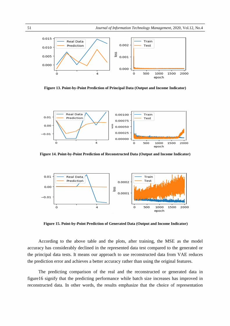
Steps of Component 3: Prediction. Since the main objective is predicting, so both data’s MSE
comparisons are rendered in Table 5 as well as the represented plots in figure 13, figure 14
and figure 15 in addition to the predicting comparison of the real and the reconstructed or
generated data in figure 16 signify that the predicting performance has improved in
reconstructed data.
Table 5. The Training Stages’ MSE Comparisons as well as Principal, Reconstructed and Generated Data Testing
Type of Data MSE for Train MSE for Test
Reconstructed Data (VAE) 6.653518159344623e-05 0.0
Generated Data (VAE) 0.00010355142347345298 0.1666666716337204
Original Data 9.459616401066093e-06 0.3333333432674408
Journal of Information Technology Management, 2020, Vol.12, No.4 51
Figure 13. Point-by-Point Prediction of Principal Data (Output and Income Indicator)
Figure 14. Point-by-Point Prediction of Reconstructed Data (Output and Income Indicator)
Figure 15. Point-by-Point Prediction of Generated Data (Output and Income Indicator)
According to the above table and the plots, after training, the MSE as the model
accuracy has considerably declined in the represented data test compared to the generated or
the principal data tests. It means our approach to use reconstructed data from VAE reduces
the prediction error and achieves a better accuracy rather than using the original features.
The predicting comparison of the real and the reconstructed or generated data in
figure16 signify that the predicting performance while batch size increases has improved in
reconstructed data. In other words, the results emphasize that the choice of representation

P-V-L Deep: A Big Data Analytics Solution for Now-casting in Monetary Policy 52
learning to achieve data quality plays an effective role in the network performance to
economic indicators prediction.
Figure 16. Point-by-Point Comparison of All above Predictions (Output and Income Indicator)
Furthermore, based on the table, the train time, testing and validation signify that LSTM
net operates better for reconstructed data compared to raw or principal data. The comparison
results are presented in Table 6.
Table 6. Train, Test and Validation’s Time Comparison of the Reconstructed, Generated and Principal Data
Type of Data Train, Test and Evaluation Time
Reconstructed Data (VAE) 32.19550395011902
Generated Data (VAE) 32.47142052650452
Original Data 34.292938232421875
Conclusion and Suggestions
Conclusion
This research has developed a novel now-casting approach through deep net and deep
learning in macro-economic area and forecasting-oriented, predictive monetary policies.
The designed P-V-L Deep: Predictive VAE-LSTM Deep net considerably promotes the
predicting performance of macro-economic indicators through two VAE and LSTM deep
architectures in unsupervised (represented) and supervised learning (now-casting and
predicting). The findings show that representation learning has a great impact on macro-
economic indicators’ predicting. In other words, the feature representation through deep
learning is very effective for huge big data. The Variational Auto-Encoder net has a great
impact on a real distribution of input features learning based on sample distribution of latent
variables and data reconstruction. Representation learning using VAE provides impressive

Journal of Information Technology Management, 2020, Vol.12, No.4 53
accuracy and better conditions for time-series now-casting models through LSTM
architecture, compared to the principal data usage in such architecture. On the other hand, this
research represents a new, data-driven approach for economic data’s now-casting modeling
with high dimensions, complexity, and sparsity of features.
This is the first now-casting model in the economics realm that has applied the VAE
advantages for feature representation and data reconstruction as well as optimizing the
performance of the reconstructed data in time-series along with LSTM architecture. This
model can be used in different economic areas based on the data-driven decision-making
approach.
The remarkable consequence of the research findings for policy-makers and executive
in policy-making institutions are as follows:
Appling deep nets to perform data quality process promotion
Reconstructing economic data instead of data revision through delay statistics or
expert analysis
Now-casting and early publication of economic indicators (with a lagging nature)
before the official release
Notable findings and implications for data scientists and information technology elites
are as follows:
Paying attention to the multi-disciplinary nature of current world issues and efforts for
transparency and comprehensiveness in the convergence of big data analytics, now-
casting, and monetary policies (or other business areas) with the goal of alignment
between strategy and big data analytics architecture. Obviously, this attention makes
promotion the level of accuracy of the policy-making institution in decision- and
policy-making
To make correct policies about how to exploit the opportunities of big data analytics
and to gain better results, human skills as the most significant progressive factor for
policy-making purposes, should be taken into account. It is recommended to invest
purposefully in earning the skills in data science incorporation to IT and business area.
Paying attention to innovations, creativities and determining proper strategies in
business can affect personnel’s’ skill level
Applying the novel methods and AI with the aim of data reconstruction instead of
traditional data revision
Consideration of the highly data-driven technologies to now-casting by using new
methods of analysis like machine learning and visualization tools with the ability of
interaction and connection to different data resources with varieties of data regarding
the type of big data aimed at reducing the risks of policy-making institution’s
investment in the field of IT
P-V-L Deep: A Big Data Analytics Solution for Now-casting in Monetary Policy 54
Consideration of non-linear relations and noises analytics in real-time data and also
exploiting new modeling tools and to consider data inclination and eventuality in
modeling
Implementing of the prediction applications with the aim of convergence of now-
casting of economic domain with big data and deep learning could be a fertile ground
for conducting the new approaches, in order for the results to help policy making
institution on the data-driven path and accurate estimates of the current state of affairs
Future Suggestions
Using the latent layer features in classifiers and comparing their performances in
classified features of other economic realm researches
The automatic selecting of represented features for LSTM input in the form of vectors
and then prediction
Using Sig Opt to make predicting model for the net’s structure’s automatic selecting
by Bayesian optimization of hyper-parameters, based on the newest research
collections in order to prevent the procedure of trial and error
Developing a decision support system based on predicting model according to
different inputs in macro-economics
Using GRU instead of LSTM and adopting performance comparison according to
topological differences, regarding the gate numbers and absence of memory unit in
GRU
Using Saiprasad Koturwar’s (2018; 2019), suggested approach instead of He (2015)
and Xavier (2010)’s suggested approach for initial weighting in deep nets based on
non-standard, unbalanced databases.
References
Alexander, L., Das, S. R., Ives, Z., Jagadish, H. V., & Monteleoni, C. (2017). Research Challenges in
Financial Data Modeling and Analysis. Michigan conference: Big Data in Finance. Michigan.
Alvarez, R. M., & Perez-Quiros, G. (2016). Aggregate versus disaggregate information in dynamic
factor models. International Journal of Forecasting, 32, 680 – 694.
Andersson, M. K., & Reijer, A. H. (2015). Nowcasting. Sveriges RIKSBANK Economic Review.
Askitas, N., & Zimmermann, K. F. (2009). Google Econometrics and Unemployment Forecasting.
Applied Economics Quarterly, 55(2), 107–120.
Atsalakis, G. S., & Valavanis, K. P. (2009). Surveying stock market forecasting techniques – Part II:
Soft computing methods. Expert Systems with Applications, 36(3), 5932-5941.
Bai, J., & Ng, S. (2008). Forecasting Economic Time Series Using Targeted Predictors. Journal of
Econometrics, 146, 304-317.

Journal of Information Technology Management, 2020, Vol.12, No.4 55
Bańbura, M., & Modugno, M. (2014). Maximum Likelihood Estimation of Factor Models on Datasets
with Arbitrary Pattern of Missing Data. Journal of Applied Econometrics, 29(1), 133-160.
Bańbura, M., Giannone, D., & Lenza, M. (2014-2015). Conditional Forecasts and Scenario Analysis
with Vector Autoregressions for Large Cross-Section. Working Papers ECARES ECARES.
Bańbura, M., Giannone, D., & Reichlin, L. (2010). Large Bayesian Vector Autoregressions. Journal of
Applied Econometrics, 25(1), 71-92.
Banerjee, A., Marcellino, M., & Masten, I. (2013). Forecasting with Factor-augmented Error
Correction Models. International Journal of Forecasting, In Press.
Bengio, Y. (2009). Learning Deep Architectures for AI. Foundations and Trends in Machine.
Bengio, Y., Courville, A., & Vincent, P. (2013). Representation learning: A review and new
perspectives. IEEE transactions on pattern analysis and machine intelligence, 35, 1798-1828.
Bernanke, B., Boivin, J., & Eliasz, P. S. (2005). Factor Augmented Vector Autoregressions (FVARs)
and the Analysis of Monetary Policy. Quarterly Journal of Economics, 120(1), 387-422.
Bernanke, B., Boivin, J., & Eliasz, P. S. (2005). Measuring the Effects of Monetary Policy: A
Factoraugmented Vector Autoregressive Approach. The Quarterly Journal of Economics,
120(1), 387-422.
Boesen, A., Larsen, L., & Sonderby, S. K. (2015). Generating Faces with Torch. Retrieved from
Torch: torch.ch/blog/2015/11/13/gan.html
Boivin, J., & Giannoni, M. (2006). DSGE Models in a Data Rich Environment. NBER Working Paper,
12272.
Bordoloi, S., Biswas, D., Singh, S., Manna, U. K., & Saggar, S. (2010). Macroeconomic Forecasting
Using Dynamic Factor Models. Reserve Bank of India Occasional Papers, 31(2), 69-83.
Bragolia, D., & Modugno, M. (2016). A Nowcasting Model for Canada: Do U.S. Variables Matter?
Finance and Economics Discussion Series 34.
Bragolia, D., & Modugno, M. (2017). Now-casting the Japanese Economy. International Journal of
Forecasting, Elsevier, 13.
Britz, D. (2015). Implementing a GRU/LSTM RNN with Python and Theano. Retrieved from Recurrent
neural network tutorial: http://www.wildml.com/2015/10/recurrent-neural-network-tutorial-part-
4-implementing-agrulstm-
Camacho, M., & Sancho, I. (2003). Spanish Diffusion Indexes. Spanish Economic Review, 5(3), 173-
203.
Carriero, A., Clark, T. E., & Marcellino, M. (2012a). Real-time Nowcasting with a Bayesian Mixed
Frequency Model with Stochastic Volatility. Federal Reserve Bank of Cleveland, Working
Paper, 1227.
Carriero, A., Kapetanios, G., & Marcellino, M. (2011). Forecasting Large Datasets with Bayesian
Reduced Rank Multivariate Models. Journal of Applied Econometrics, 26(5), 735-761.
Carriero, A., Kapetanios, G., & Marcellino, M. (2012b). Forecasting government bond yields with
large Bayesian Vector Autoregressions. Journal of Banking & Finance, 36(7), 2026-2047.
Charte, D., Charte, F., Garc´ıa, S., Jesus, M. J., & Herrera, F. (2018). A practical tutorial on
autoencoders for nonlinear feature fusion: Taxonomy, models, software and guidelines.

P-V-L Deep: A Big Data Analytics Solution for Now-casting in Monetary Policy 56
Chernis, T., & Sekkel, R. (2017). A Dynamic Factor Model for Nowcasting Canadian GDP Growth.
Bank of Canada Staff Working Paper, 2.
Choi, H., & Varian, H. (2012). Predicting the Present with Google Trends. Economic Record, 88(s1),
2-9.
Chollet, F. (2016). Keras. Retrieved from Github: https://github.com/fchollet/keras
Dai, H., Tian, Y., Dai, B., Skiena, S., & Song, L. (2018). Syntax -Directed Variational Autoencoder
For Structured Data. arXiv:1802.08786v1.
Deng, L., & Yu, D. (2014). Deep learning: methods and applications. Foundations and Trends in
Signal Processing, 7, 197-387.
Diebold, F. X. (2003). Big Data Dynamic Factor Models for Macroeconomic Measurement and
Forecasting. (M. Dewatripont, L. P. Hansen, & S. Turnovsky, Eds.) Advances in Economics and
Econometrics, Eighth World Congress of the Econometric Society, 115-122.
Diederik, P. K., & Welling, M. (2013). Auto-Encoding Variational Bayes. arXiv:1312.6114.
Dixon, M., Klabjan, D., & Bang, J. H. (2015). Implementing deep neural networks for financial
market prediction on the Intel Xeon Phi. Proceedings of the 8th Workshop on High
Performance Computational Finance, (pp. 1-6).
Doersch, C. (2016). Tutorial on variational autoencoders. arXiv preprint arXiv:1606.05908.
Domingos, P. (2015). The Master Algorithm: How the Quest for the Ultimate Learning Machine Will
Remake Our World. In Deeper into the Brain.
Doz, C., Giannone, D., & Reichlin, L. (2012). A quasi–maximum likelihood approach for large,
approximate dynamic factor models. Review of Economics and Statistics, 94, 1014–1024.
Duarte, C., Rodrigues, P. M., & Rua, A. (2017). A Mixed Frequency Approach To The Forecasting Of
Private Consumption With ATM/POS Data. International Journal of Forecasting, Elsevier, 15.
Elaraby, N. M., Elmogy, M., & Barakat, S. (2016). Deep Learning: Effective Tool for Big Data
Analytics. International Journal of Computer Science Engineering (IJCSE), 9.
Fan, J., Han, F., & Liu, H. (2014). Challenges of Big Data Analysis. National Science Review, 1(2),
293-314.
Federal Reserved Bank. (2017). Nowcasting Report. The FRBNY Staff Nowcast.
Figueiredo, F. R. (2010). Forecasting Brazilian Inflation using a Large Dataset. Central Bank of
Brazil, Working Paper, 228. Retrieved from http://www.bcb.gov.br/pec/wps/ingl/wps228.pdf
Fischer, T., & Krauss, C. (2017). Deep learning with long short-term memory networks for financial
market predictions. FAU Discussion Papers in Economics.
Forni, M., Hallin, M., Lippi, M., & Reichlin, L. (2005). The Generalized Dynamic Factor Model:
OneSided Estimation and Forecasting. Journal of the American Statistical Association,
100(471), 830-840.
Gal, Y., & Ghahramani, Z. (2016). A theoretically grounded application of dropout in recurrent neural
networks. Advances in Neural Information Processing Systems, 1019-1027.
Galbraith, J. W., & Tkacz, G. (2016). Nowcasting with Payments System Data. International Journal
of Forecasting, Elsevier.
Journal of Information Technology Management, 2020, Vol.12, No.4 57
Galeshchuk, S., & Mukherjee, S. (2017). Deep Learning for Predictions in Emerging Currency
Markets. the 9th International Conference on Agents and Artificial Intelligence, Science and
Technology. ResearchGate. doi:10.5220/0006250506810686
Gavidel, S. Z., & Rickli, J. L. (2017). Quality assessment of used-products under uncertain age and.
International Journal of Production Research, 1-15.
Gers, F. A., Schmidhuber, J., & Cummins, F. (2000). Learning to forget: Continual prediction with
LSTM. Neural computation, 12(10), 2451-2471.
Ginsberg, J., Mohebbi, M., H, M., Patel, R. S., Brammer, L., Smolinski, M. S., & Brilliant, L. (2009).
Detecting influenza epidemics using search engine query data. Nature, 457(7232), 1012–14.
Giovanelli, A. (2012). Nonlinear Forecasting using Large Datasets: Evidence on US and Euro Area
Economies. CEIS Tor Vergata, 10(13), 1-29. Retrieved from
http://papers.ssrn.com/sol3/papers.cfm?abstract_id=2172399
Girin, L., Hueber, T., Roche, F., & Leglaive, S. (2019). Notes On The Use Of Variational
Autoencoders For Speech And Audio. the 22nd International Conference on Digital Audio
Effects. Birmingham. Retrieved from http://www.gipsa-lab.fr/~laurent.girin/papers/Girin_et_al_
DAFx2019.pdf
Global Pluse. (2013). Mobile Phone Network Data. United Nations Global Pluse, 1-12.
Glorot, X., & Bengio, Y. (2010). Understanding the difficulty of training deep feedforward neural
networks. Aistats, 9.
Goel, S., Hofman, J. M., Lahaie, S., Pennock, D. M., & Watts, D. J. (2010). Predicting consumer
behavior with Web search. Proceedings of the National Academy of Sciences of the United
States of America, 107(41), 17486–90.
Graves, A. (2014). Generating sequences with recurrent neural networks. arXiv preprint
arXiv:1308.0850.
Graves, A., & Schmidhuber, J. (2005). Framewise phoneme classification with bidirectional LSTM
and other neural network architectures. Neural Networks, 602-610.
Graves, A., Liwicki, M., Fern´ andez, S., Bertolami, R., Bunke, H., & Schmidhuber, J. (2009). A novel
connectionist system for unconstrained handwriting recognition. IEEE transactions on pattern
analysis and machine intelligence, 31(5), 855-868.
Graves, A., Mohamed, A. -r., & Hinton, G. (2013). Speech recognition with deep recurrent neural
networks. IEEE international conference on acoustics, speech and signal processing, (pp. 6645-
6649).
Green, J., Hand, J. R., & Zhang, X. F. (2013). The supraview of return predictive signals. Review of
Accounting Studies, 18(3), 992-730.
Gupta, R., Kabundi, A., Miller, S., & Uwilingiye, J. (2013). Using Large Datasets to Forecast Sectoral
Unemployment. Statistical Methods & Applications, forthcoming.
Han, K., Zhang, C., Li, C., & Xu, C. (2018). Autoencoder Inspried Unsupervised Feature Selection.
IEEE International Conference on Acoustics, Speech and Signal Processing (ICASSP).
ResearchGate.
Hassani, H., & Silva, E. S. (2015). Forecasting with Big Data: A Review. Annals of Data Science, 20.

P-V-L Deep: A Big Data Analytics Solution for Now-casting in Monetary Policy 58
He, K., Zhang, X., Ren, S., & Sun, J. (2015). Delving deep into rectifiers: Surpassing human-level
performance on imagenet classification. Proceedings of the IEEE international conference on
computer vision.
Hindrayanto, I., JanKoopman, S., & Winter, J. d. (2016). Forecasting and Nowcasting Economic
Growth in the Euro Area Using Factor Models. International Journal of Forecasting, Elsevier,
22.
Hinton, G. E. (2009). Deep belief networks. Scholarpedia, 4(5947).
Hochreiter, S., & Schmidhuber, J. (1997). Long short-term memory. Neural computation, 9(8), 1735-
1780.
Hoog, S. V. (2016). Deep Learning in Agent-Based Models: A Prospectus. Working Papers in
Economics and Management, 19.
Hsu, Y.-C., & Kira, Z. (2016). NEURAL NETWORK-BASED CLUSTERING USING PAIR-WISE
CONSTRAINTS. arXiv:1511.06321v5.
Huck, N. (2009). Pairs selection and outranking: An application to the S&P 100 index. European
Journal of Operational Research, 196(2), 819-825.
Huck, N. (2010). Pairs trading and outranking: The multi-step-ahead forecasting case. European
Journal of Operational Research, 207(3), 1702–1716.
Jacobs, H. (2015). What explains the dynamics of 100 anomalies? Journal of Banking & Finance.
Jagadish, H. V., Gehrke, J., Papakonstantinou, A., Patel, Y., Ramakrishnan, R., & Shahabi, C. (2014).
Big data and its technical challenges. Communications of the ACM, 57(7), 86-94.
Jurado, K., Ludvigson, S., & Ng, S. (2015). Measuring Macroeconomic Uncertainty. American
Economic Review, 105(3), 1177-1216.
Kapetanios, G., & Marcellino, M. (2009). A Parametric Estimation Method for Dynamic Factor
Models of Large Dimensions. Journal of Time Series Analysis, 30(2), 208-238.
Kapetanios, G., Marcellino, M., & Papailias, F. (2016). Big Data and Macroeconomic Nowcasting.
European Commission, Worldwide Consultants, 79.
Karpathy, A. (2015). The unreasonable effectiveness of recurrent neural networks. Retrieved from
Github: http://karpathy.github.io/2015/05/21/rnn-effectiveness/
Karray, F., Campilho, A., & Yu, A. (Eds.). (2019). Image Analysis and Recognition: 16th
International Conference. Waterloo, ON, Canada: Springer.
Kingma, D., & Welling, M. (2019). An Introduction to Variational Autoencoders. Foundations and
Trends in Machine Learning, 12, 307-392. doi:10.1561/2200000056
Koop, G. M. (2013). Forecasting with Medium and Large Bayesian VARs. Journal of Applied
Econometrics, 28(2), 177-203.
Koturwar, S., & Merchant, S. (2019). Weight Initialization of Deep Neural Networks(DNNs) Using
Data Statistics. Retrieved from ResearchGate:
https://www.researchgate.net/publication/320727084_Weight_Initialization_of_Deep_Neural_
Net
Koturwar, S., & Merchant, S. N. (2018). Weight Initialization of Deep Neural Networks(DNNs) Using
Data Statistics. Elsevier, arXiv:1710.10570v2.
Journal of Information Technology Management, 2020, Vol.12, No.4 59
Krauss, C., Do, X. A., & Huck, N. (2017). Deep neural networks, gradient-boosted trees, random
forests Statistical arbitrage on the S&P 500. European Journal of Operational Research, 259(2),
689-702.
Kroft, K., & Pope, D. G. (2014). Does Online Search Crowd Out Traditional Search and Improve
Matching Efficiency? Journal of Labor Economics, 32(2), 259–303.
Kuhn, P., & Mansour, H. (2014). Is Internet Job Search Still Ineffective? Economic Journal, 124(581),
1213–1233.
Kuhn, P., & Skuterud, M. (2004). Internet Job Search and Unemployment Durations. American
Economic, Review, 94(1), 218–232.
Lahiri, K., & Monokroussos, G. (2013). Nowcasting US GDP: The role of ISM business surveys.
International Journal of Forecasting, 29, 644–658.
Lahiri, K., Monokroussos, G., & Zhao, Y. (2015). Forecasting Consumption: the Role of Consumer
Confidence in Real-time with many Predictors. Journal of Applied Econometrics.
Le, X.-H., Viet Ho, H., Lee, G., & Jung, S. (2019). Application of Long Short-Term Memory (LSTM)
Neural Network for Flood Forecasting. Water, 11(1387).
LeCun, Y., Bengio, Y., & Hinton, G. (2015). Deep learning. Nature, 521, 436–444.
Lee, H., Ekanadham, C., & Ng, A. (2008). Sparse deep belief net model for visual area v2. (J. Platt, D.
Koller, Y. Singer, & S. Roweis, Eds.) Advances in neural information processing systems, 20,
873-880.
Li, R., Li, X., Lin, C., Collinson, M., & Mao, R. (2019). A Stable Variational Autoencoder for Text
Modelling. Proceedings of The 12th International Conference on Natural Language Generation
(pp. 594–599). Tokyo: Association for Computational Linguistics. Retrieved from
https://www.aclweb.org/anthology/W19-8673.pdf
Li, X. (2016). Nowcasting with Big Data: is Google useful in Presence of other Information? London
Business School.
Liangchen, W., & Deng, Z.-H. (2017). Variational Autoencoding Approach for Inducing Cross-lingual
Word. The Twenty-Sixth International Joint Conference on Artificial Intelligence.
Louizos, C., Shalit, U., & Mooij, J. (2017). Causal Effect Inference with Deep Latent-Variable
Models. arXiv:1705.08821v2.
Lu, M. (2019). A monetary policy prediction model based on deep learning. Neural Computing and
Applications, 5649–5668.
Ludvigson, S., & Ng, S. (2011). A Factor Analysis of Bond Risk Premia. Handbook of Empirical
Economics and Finance. (D. Gilles, & A. Ullah, Eds.)
Mamoshina, P., Vieira, A., Putin, E., & Zhavoronkov, A. (2016). Applications of deep learning in
biomedicine. Molecular pharmaceutics, 13, 1445-1454.
Marcellino, M., Stock, J., & Watson, M. (2006). A Comparison of Direct and Iterated AR Methods for
Forecasting Macroeconomic Time Series h-steps Ahead. Journal of Econometrics, 135, 499-
526.
McCracken, M. W., & Ng, S. (2015). FRED-MD: A Monthly Database for Macroeconomic Research.
Research Division-Federal Reserve Bank of St. Louis, Working Paper Series. Retrieved from
http://research.stlouisfed.org/wp/2015/2015-012.pdf
P-V-L Deep: A Big Data Analytics Solution for Now-casting in Monetary Policy 60
Medsker, J. (2000). Recurrent Neural Networks: Design and Applications. International Series on
Computational Intelligence.
Mendels, G. (2019). Selecting the right weight initialization for your deep neural network. Data
Science.
Miotto, R., Wang, F., Jiang, X., & Dudley, J. T. (2018). Deep learning for healthcare: review,
opportunities and challenges. Briefings in Bioinformatics. doi:10.1093/bib/bbx044
Mol, C. D., Giannone, D., & Reichlin, L. (2008). Forecasting using a Large Number of Predictors: Is
Bayesian Shrinkage a Valid Alternative to Principal Components? Journal of Econometrics,
146(2), 318-328.
Moradi-Aliabadi, M., & Huang, Y. (2016). Multistage optimization for chemical process
sustainability. ACS Sustainable Chemistry & Engineering.
Moritz, B., & Zimmermann, T. (2014). Deep conditional portfolio sorts: The relation between past and
future stock returns. Working paper, LMU Munich and Harvard University.
Najafabadi, M., Villanustre, F., Khoshgoftaar, T., Seliya, N., Wald, R., & Muharemagic, E. (2015).
Deep learning applications and challenges in big data analytics. Journal of Big Data,
SpringerOpen, 2(1). doi:10.1186/s40537-014-0007-7
Njuguna, C. P. (2017). Constructing spatiotemporal poverty indices from big data. Journal of Business
Research, Elsevier, 10.
Nymand-Andersen, P. (2015). The use of Google Search data for macro-economic nowcasting. CCSA,
Europen Central Banks, EuroSystem, 16.
Nymand-Andersen, P. (2016). Big data: The hunt for timely insights and decision certainty. IFC
Working Papers, Bank for International Settlements, 14. Retrieved from www.bis.org
Olah, C. (2015). Understanding LSTM Networks. Retrieved from http://colah.github.io/posts/2015-08-
Understanding-LSTMs/
Ostapenko, N. (2020). Identification of Monetary Policy Shocks from FOMC Transcripts. SSRN.
Retrieved from https://ssrn.com/abstract=3527415
Ouysse, R. (2013). Forecasting using a Large Number of Predictors: Bayesian Model Averaging
versus Principal Components Regression. Australian School of Business Research Paper,
2013ECON04, 1-34. Retrieved from http://research.economics.unsw.edu.au/RePEc/papers/
2013-04.pdf
Partaourides, H., & Chatzis, S. P. (2017). Asymmetric deep generative models. Neurocomputing,
241(90). doi:10.1016/j.neucom.2017.02.028
Rajkomar, A., Oren, E., & Chen, K. (2018). Scalable and accurate deep learning with electronic health
records. Nature. Retrieved from https://www.nature.com/articles/s41746-018-0029-1
Rezende, D. J., Mohamed, S., & Wierstra, D. (2014). Stochastic backpropagation and approximate
inference in deep generative models. In Proceedings of the 31st International Conference on
Machine Learning (ICML-14), (pp. 1278-1286).
Rocca, J. (2019). Understanding Variational Autoencoders (VAEs). Data Science.
Roostaei, J., & Zhang, Y. (2016). Spatially explicit life cycle assessment: Opportunities and
challenges. Algal Research.

Journal of Information Technology Management, 2020, Vol.12, No.4 61
Sak, H., Senior, A., & Beaufays, F. (2014). Long short-term memory based recurrent neural network
architectures for large vocabulary speech recognition. arXiv preprint arXiv:1402.1128.
Schmidhuber, J. (2015). Deep learning in neural networks: An overview. Neural Networks, 61.
Sermpinis, G., Theofilatos, K., Karathanasopoulos, A., Georgopoulos, E. F., & Dunis, C. (2013).
Forecasting foreign exchange rates with adaptive neural networks using radial-basis functions
and particle swarm optimization. European Journal of Operational Research, 225(3), 528–540.
Shuyang, D., Pandey, M., & Xing, C. (2017). Modeling approaches for time series forecasting and
anomaly detection. Standford. ArXiv.
Simidjievski, N., Bodnar, C., Tariq, I., Scherer, P., Andres Terre, H., Shams, Z., . . . Liò, P. (2019).
Variational Autoencoders for Cancer Data Integration: Design Principles and Computational
Practice. Bioinformatics and Computational Biology, a section of the journal Frontiers in
Genetics, 10. doi:10.3389/fgene.2019.01205
Soto, V., Frias-Martinez, V., Virseda, J., & Frias-Martinez, E. (2011). Prediction of socioeconomic
levels using cell phone records. Lect. Notes Comput. Sci., 6787 LNCS(1), 377 –388.
Staudemeyer, R., & Morris, E. (2019). Understanding LSTM -- a tutorial into Long Short-Term
Memory Recurrent Neural Networks. ResearchGate. Retrieved from
https://www.researchgate.net/publication/335975993
Stevenson, B. (2008). The Internet and Job Search. NBER Working Paper 13886.
Stock, J. H., & Watson, M. W. (1996). Evidence on Structural Instability in Macroeconomic Time
Series Relations. Journal of Business and Economic Statistics, 11-30.
Stock, J. H., & Watson, M. W. (1998). Diffusion Indexes. NBER Working Paper, 6702.
Stock, J. H., & Watson, M. W. (2002). Macroeconomic Forecasting Using Diffusion Indexes. Journal
of Business and Economic Statistics, 20(2), 47-162.
Stock, J., & Watson, M. W. (2005). Implications of Dynamic Factor Models for VAR analysis. NBER
Working Paper, 11467.
Stock, J., & Watson, M. W. (2006). Forecasting with Many Predictors, Handbook of Forecasting.
North Holland.
Suk, H.-I., Lee, S.-W., & Shen, D. (2016). Latent feature representation with stacked auto-encoder for
AD/MCI diagnosis. Brain Structure and Function, 220(2), 841-859.
Takeuchi, L., & Lee, Y. -Y. (2013). Applying deep learning to enhance momentum trading strategies
in stocks. Working paper, Stanford University.
Thiemann, P. G. (2016). Big Data: Bringing Competition Policy to the Digital Era. OEDC -
Organisation for Economic Co-operation and Development, 40.
Tieleman, T., & Hinton, G. (2012). Lecture 6.5-rmsprop: Divide the gradient by a running average of
its recent magnitude. COURSERA: Neural Networks for Machine Learning, 4(2), 26-31.
Tiffin, A. (2016). Seeing in the Dark: A Machine-Learning Approach to Nowcasting in Lebanon. IMF
Working Paper, 20.
Tozzi, C. (2018). Big Data Trends: Liberate, Integrate & Trust, eBook. Syncsort. Retrieved from
Available at: https://blog.syncsort.com/2018/02/big-data/big-data-use-cases-2018/
Tuhkuri, J. (2014). Big Data: Google Searches Predict Unemployment in Finland. ETLA Reports, 31.
P-V-L Deep: A Big Data Analytics Solution for Now-casting in Monetary Policy 62
Tuhkuri, J. (2016). A Model for Forecasting with Big Data - Forecasting Unemployment with Google
Searches in Europe. Elsevier, 54(20).
Varian, H. (2018). Retrieved from https://www.youtube.com/watch?v=aUl OVgT Y
Vincent, P., Larochelle, H., Lajoie, I., Bengio, Y., & Manzagol, P.-A. (2010). Stacked Denoising
Autoencoders: Learning Useful Representations in a Deep Network with a Local. The Journal
of Machine Learning Research, 11, 371-3408.
Wang, H., Xu, Z., Fujita, H., & Liu, S. (2016). Towards felicitous decision making: An overview on
challenges and trends of Big Data. Information Sciences, Science Direct, Elsevier, 19.
Wong, W.-k., Shi, X. J., Yeung, D. Y., & Woo, W.-C. (2016). A deep-learning method for
precipitation nowcasting. WMO WWRP 4th International Symposium on Nowcasting and Very-
short-range Forecast 2016. Hong Kong.
Wu, L., & Brynjolfsson, E. (2015). The Future of Prediction: How Google Searches Foreshadow
Housing Prices and Sales. (A. Goldfarb, S. Greenstein, & C. Tucker, Eds.) Economic Analysis
of the Digital Economy, 89–118.
Yasir, M., Afzal, S., Latif, K., Chaudhary, G., Malik, N., Shahzad, F., & Song, O.-y. (2020). An
Efficient Deep Learning Based Model to Predict Interest Rate Using Twitter Sentiment.
Sustainability. doi:10.3390
Zafar Nezhad, M., Zhu, D., Li, X., Yang, K., & Levy, P. (2017). SAFS: A Deep Feature Selection.
arXiv:1704.05960v1.
Zafar Nezhad, M., Zhu, D., Sadati, N., & Yang, K. (2018). A Predictive Approach Using Deep Feature
Learning for Electronic Medical Records: A Comparative Study. arXiv:1801.02961v1.
Zafar Nezhad, M., Zhu, D., Sadati, N., Yang, K., & Levy, P. (2017). A supervised bi-clustering
approach for precision medicine. arXiv preprint arXiv:1709.09929.
Bibliographic information of this paper for citing:
Hajipour Sarduie, M., Afshar Kazemi, M., Alborzi, M., Azar, A., & Kermanshah, A. (2020). P-V-L Deep: A Big
Data Analytics Solution for Now-casting in Monetary Policy. Journal of Information Technology Management,
12(4), 22-62.
Copyright © 2020, Maryam Hajipour Sarduie, Mohammadali Afshar Kazemi, Mahmood Alborzi, Adel Azar and Ali
Kermanshah.