Compiler  Op+miza+on  for  Heterogeneous  Systems  

P.  (Saday)  Sadayappan  The  Ohio  State  University  

The Good Old Days for Software Source: J. Birnbaum

•  Single-processor performance experienced dramatic improvements from clock, and architectural improvement (Pipelining, Instruction-Level-Parallelism)

•  Applications experienced automatic performance improvement

3

WaA

s/cm

2

1

10

100

1000

1.5µ 1µ 0.7µ 0.5µ 0.35µ 0.25µ 0.18µ 0.13µ 0.1µ 0.07µ

i386 i486

Pen+um®   Pen+um®  Pro  

Pen+um®  II  Pen+um®  III  Hot plate

Rocket Nozzle Nuclear Reactor

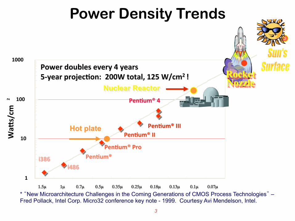
* “New Microarchitecture Challenges in the Coming Generations of CMOS Process Technologies” – Fred Pollack, Intel Corp. Micro32 conference key note - 1999. Courtesy Avi Mendelson, Intel.

Pen+um®  4  

Power Density Trends

Power  doubles  every  4  years  5-­‐year  projec+on:    200W  total,  125  W/cm2  !  

4

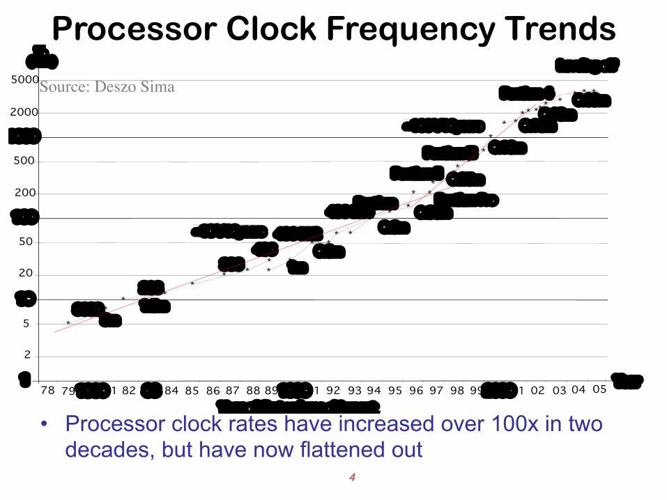
Processor Clock Frequency Trends

4

5

10

50

Year

*

**

*

2

8088

*

100

386

Pentium

Year of first volume shipment

cf

500

1000

20

200

*

486-DX2

79 198081 82 83 84 85 86 87 88 89199091 92 93 94 95 96 97 98 9978

3m

*1.5m

*

**

*

*486 0.8m

*

** *

*

0.35m

** *

**

0.25mPentium II

***Pentium III

*

286

*

Pentium Pro

1

1m

0.6m

486-DX4

200001 02 03

2000**

***

***

*

*

5000

0.18m0.13m

Pentium 4

0.18m

~10*/10years

~100*/10years

04 05

* * *0.09m

Leveling off(MHz)

•  Processor clock rates have increased over 100x in two decades, but have now flattened out

Source: Deszo Sima

5

Single-Processor Performance Trends

5

1

10

100

1000

10000

100000

1978 1980 1982 1984 1986 1988 1990 1992 1994 1996 1998 2000 2002 2004 2006 2008 2010 2012 2014 2016

Per

form

ance

(vs.

VA

X-1

1/78

0)

25%/year

52%/year

Source: Hennessy and Patterson, Computer Architecture: ���A Quantitative Approach

•  Single-processor performance improved by about 50% per year for almost two decades, but has now flattened out: limited further upside from clock or ILP

6

Moore’s Law: Still Going Strong

6

1

10

100

1000

10000

100000

1978 1980 1982 1984 1986 1988 1990 1992 1994 1996 1998 2000 2002 2004 2006 2008 2010 2012 2014 2016

Per

form

ance

(vs.

VA

X-1

1/78

0)

25%/year

52%/year

??%/year

8086  

286  386  

486  Pen+um  

P2  P3  P4  

Itanium  Itanium  2  

1,000,000,000  

100,000  

10,000  

1,000,000  

10,000,000  

100,000,000  

Source: Saman Amarasinghe

Num

ber  of  Transistors  

•  But transistor density continues to rise unabated •  Multiple cores are now the best option for sustained

performance growth

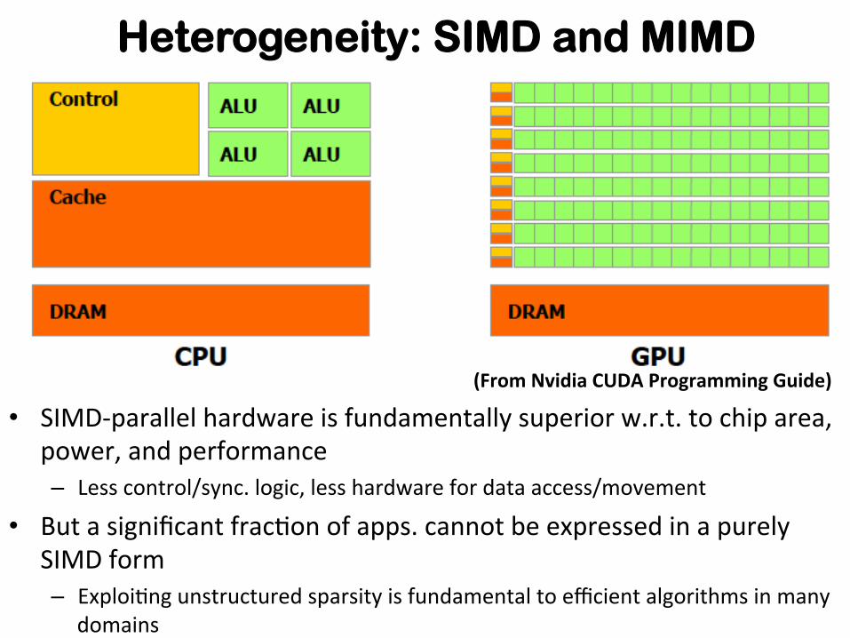
Heterogeneity: SIMD and MIMD

•  SIMD-­‐parallel  hardware  is  fundamentally  superior  w.r.t.  to  chip  area,  power,  and  performance  –  Less  control/sync.  logic,  less  hardware  for  data  access/movement  

•  But  a  significant  frac+on  of  apps.  cannot  be  expressed  in  a  purely  SIMD  form  –  Exploi+ng  unstructured  sparsity  is  fundamental  to  efficient  algorithms  in  many  

domains  

(From  Nvidia  CUDA  Programming  Guide)  

GPU vs. CPU Performance

Source:  NVIDIA  

Future Hardware Heterogeneity

Source: Jack Dongarra

Domain-Specific Optimization

•  Heterogeneity  creates  a  soTware  challenge  – Mul+ple  implementa+ons  for  different  system  components,  e.g.  OpenMP  (mul+-­‐core),  OpenCL  (GPU),  VHDL  (FPGA)  

•  How  can  we  Write-­‐Once-­‐Execute-­‐Anywhere?  –  Too  daun+ng  a  challenge  for  general-­‐purpose  languages  – More  promising  for  domain-­‐specific  approaches  

•  Three  examples  of  domain-­‐specific  computa+onal  abstrac+ons  –  Stencil  computa+ons  –  Tensor  expressions  – Affine  computa+ons  

Domain-Specific Examples

•  Stencil  computa+ons  •  Tensor  expressions  •  Affine  computa+ons  

Domain Example: Stencil Computations

x_dis_tmp[i][j] = a*(x_dis[i][j] – dt*tmp2*(tmp1 - img1[i][j])) - b*(x_dis[i ][j+2] - 6*x_dis[i ][j+1] - 6*x_dis[i ][j-1] + x_dis[i ][j-2] + x_dis[i+2][j ] – 6*x_dis[i+1][j ] – 6*x_dis[i-1][j ] + x_dis[i-2][j ] + x_dis[i+1][j+1] + x_dis[i+1][j-1] + x_dis[i-1][j+1] + x_dis[i-1][j-1] );  

12  

Vectorizing Stencil Computations •  Fundamental source of inefficiency

with current short-vector SIMD ISAs –  Each data element is reused in different

“slots” of vector register –  Redundant loads or shuffle ops needed

•  Two complementary approaches pursued to address problem –  Data layout transformation –  Architecture customization

for (i = 0; i < H; ++i) for (j = 0; j < W; ++j) c[i][j] = b[i][j] + b[i][j+1];

m

a b c d e f g h i j Data in Memory:

n o p q r s t u v

Vector Registers

m n o p

n o p q

a b c dVR1

VR2

VR3

VR4

VR5

0 1 2 3

k l

w x

c[i][j] b[i][j]

Inefficiency: each element of b is loaded twice

Data Layout Transformation

(a) 1D vector in memory ó (b) 2D logical view of same data (c) Transposed 2D array moves interacting elements into same slot of different vectors ó (d) New 1D layout after transformation •  Boundaries need special handling •  More details in paper at CC’11

for (j = 1; j < W-1; ++j) z[j] = y[j-1] + y[j] + y[j+1];

y[0:23]

yt[0:23]

Handling Boundaries

•  Upper and lower boundaries computed using shuffles and masked stores

•  Steady state requires no shuffles (O(n) shuffles without layout transform)

Higher Dimensional Stencils

•  Only transform fastest varying dimension of array •  Neighbor points still in corresponding vector slots •  Pad fastest varying dimension if necessary

0

2

4

6

8

10

12

14

16 P

heno

m

Cor

e2Q

uad

Cor

e i7

Phe

nom

Cor

e2Q

uad

Cor

e i7

Phe

nom

Cor

e2Q

uad

Cor

e i7

Phe

nom

Cor

e2Q

uad

Cor

e i7

Phe

nom

Cor

e2Q

uad

Cor

e i7

Phe

nom

Cor

e2Q

uad

Cor

e i7

Phe

nom

Cor

e2Q

uad

Cor

e i7

J-1D J-2D-5pt J-2D-9pt J-3D Heatttut-3D FDTD-2D Rician-2D

Gflo

p/s

Benchmark / Microarchitecture

DLT Experimental Evaluation

Ref.

DLT

DLTi

Domain-Specific Examples

•  Stencil computations •  Tensor expressions •  Affine computations

The Tensor Contraction Engine A Domain-Specific Compiler for Many-Body Methods in Quantum Chemistry

Oak Ridge National Laboratory

David E. Bernholdt, Robert Harrison

Pacific Northwest National Laboratory

Jarek Nieplocha

Louisiana State University Gerald Baumgartner J. Ramanujam

Ohio State University Xiaoyang Gao, Albert Hartono, Sriram Krishnamoorthy, Qingda Lu, Alex Sibiryakov, Russell Pitzer, P. Sadayappan

University of Florida

So Hirata

University of Waterloo

Marcel Nooijen

Supported by NSF and DOE

Time Crunch in Quantum Chemistry

Two major bottlenecks in computational chemistry: •  Very computationally intensive models •  Extremely time consuming to develop codes The vicious cycle of computational science: •  More powerful computers make more accurate models computationally

feasible :-) •  But efficient parallel implementation of complex models takes longer and

longer •  Hence computational scientists spend more time with MPI programming,

and less time doing science :-( •  Coupled Cluster family of models

in electronic structure theory •  Increasing number of terms =>

explosive increase in code complexity

•  Theory well known for decades but efficient implementations took many years

1992 79901 183 CCSDTQ

1988 33932 102 CCSDT

1982 13213 48 CCSD

1978 3209 11 CCD

Year #F77Lines #Terms Theory

CCSD Doubles Equation (Quantum Chemist’s Eye Test Chart :-) hbar[a,b,i,j] == sum[f[b,c]*t[i,j,a,c],{c}] -sum[f[k,c]*t[k,b]*t[i,j,a,c],{k,c}] +sum[f[a,c]*t[i,j,c,b],{c}] -sum[f[k,c]*t[k,a]*t[i,j,c,b],

{k,c}] -sum[f[k,j]*t[i,k,a,b],{k}] -sum[f[k,c]*t[j,c]*t[i,k,a,b],{k,c}] -sum[f[k,i]*t[j,k,b,a],{k}] -sum[f[k,c]*t[i,c]*t[j,k,b,a],{k,c}] +sum[t[i,c]*t[j,d]*v[a,b,c,d],{c,d}] +sum[t[i,j,c,d]*v[a,b,c,d],{c,d}] +sum[t[j,c]*v[a,b,i,c],{c}] -sum[t[k,b]*v[a,k,i,j],{k}] +sum[t[i,c]*v[b,a,j,c],{c}] -sum[t[k,a]*v[b,k,j,i],{k}] -sum[t[k,d]*t[i,j,c,b]*v[k,a,c,d],{k,c,d}] -sum[t[i,c]*t[j,k,b,d]*v[k,a,c,d],{k,c,d}] -sum[t[j,c]*t[k,b]*v[k,a,c,i],{k,c}] +2*sum[t[j,k,b,c]*v[k,a,c,i],{k,c}] -sum[t[j,k,c,b]*v[k,a,c,i],{k,c}] -sum[t[i,c]*t[j,d]*t[k,b]*v[k,a,d,c],{k,c,d}] +2*sum[t[k,d]*t[i,j,c,b]*v[k,a,d,c],{k,c,d}] -sum[t[k,b]*t[i,j,c,d]*v[k,a,d,c],{k,c,d}] -sum[t[j,d]*t[i,k,c,b]*v[k,a,d,c],{k,c,d}] +2*sum[t[i,c]*t[j,k,b,d]*v[k,a,d,c],{k,c,d}] -sum[t[i,c]*t[j,k,d,b]*v[k,a,d,c],{k,c,d}] -sum[t[j,k,b,c]*v[k,a,i,c],{k,c}] -sum[t[i,c]*t[k,b]*v[k,a,j,c],{k,c}] -sum[t[i,k,c,b]*v[k,a,j,c],{k,c}] -sum[t[i,c]*t[j,d]*t[k,a]*v[k,b,c,d],{k,c,d}] -sum[t[k,d]*t[i,j,a,c]*v[k,b,c,d],{k,c,d}] -sum[t[k,a]*t[i,j,c,d]*v[k,b,c,d],{k,c,d}] +2*sum[t[j,d]*t[i,k,a,c]*v[k,b,c,d],{k,c,d}] -sum[t[j,d]*t[i,k,c,a]*v[k,b,c,d],{k,c,d}] -sum[t[i,c]*t[j,k,d,a]*v[k,b,c,d],{k,c,d}] -sum[t[i,c]*t[k,a]*v[k,b,c,j],{k,c}] +2*sum[t[i,k,a,c]*v[k,b,c,j],{k,c}] -sum[t[i,k,c,a]*v[k,b,c,j],{k,c}] +2*sum[t[k,d]*t[i,j,a,c]*v[k,b,d,c],{k,c,d}] -sum[t[j,d]*t[i,k,a,c]*v[k,b,d,c],{k,c,d}] -sum[t[j,c]*t[k,a]*v[k,b,i,c],{k,c}] -sum[t[j,k,c,a]*v[k,b,i,c],{k,c}] -sum[t[i,k,a,c]*v[k,b,j,c],{k,c}] +sum[t[i,c]*t[j,d]*t[k,a]*t[l,b]*v[k,l,c,d],{k,l,c,d}] -2*sum[t[k,b]*t[l,d]*t[i,j,a,c]*v[k,l,c,d],{k,l,c,d}] -2*sum[t[k,a]*t[l,d]*t[i,j,c,b]*v[k,l,c,d],{k,l,c,d}] +sum[t[k,a]*t[l,b]*t[i,j,c,d]*v[k,l,c,d],{k,l,c,d}] -2*sum[t[j,c]*t[l,d]*t[i,k,a,b]*v[k,l,c,d],{k,l,c,d}] -2*sum[t[j,d]*t[l,b]*t[i,k,a,c]*v[k,l,c,d],{k,l,c,d}] +sum[t[j,d]*t[l,b]*t[i,k,c,a]*v[k,l,c,d],{k,l,c,d}] -2*sum[t[i,c]*t[l,d]*t[j,k,b,a]*v[k,l,c,d],{k,l,c,d}] +sum[t[i,c]*t[l,a]*t[j,k,b,d]*v[k,l,c,d],{k,l,c,d}] +sum[t[i,c]*t[l,b]*t[j,k,d,a]*v[k,l,c,d],{k,l,c,d}] +sum[t[i,k,c,d]*t[j,l,b,a]*v[k,l,c,d],{k,l,c,d}] +4*sum[t[i,k,a,c]*t[j,l,b,d]*v[k,l,c,d],{k,l,c,d}] -2*sum[t[i,k,c,a]*t[j,l,b,d]*v[k,l,c,d],{k,l,c,d}] -2*sum[t[i,k,a,b]*t[j,l,c,d]*v[k,l,c,d],{k,l,c,d}] -2*sum[t[i,k,a,c]*t[j,l,d,b]*v[k,l,c,d],{k,l,c,d}] +sum[t[i,k,c,a]*t[j,l,d,b]*v[k,l,c,d],{k,l,c,d}] +sum[t[i,c]*t[j,d]*t[k,l,a,b]*v[k,l,c,d],{k,l,c,d}] +sum[t[i,j,c,d]*t[k,l,a,b]*v[k,l,c,d],{k,l,c,d}] -2*sum[t[i,j,c,b]*t[k,l,a,d]*v[k,l,c,d],{k,l,c,d}] -2*sum[t[i,j,a,c]*t[k,l,b,d]*v[k,l,c,d],{k,l,c,d}] +sum[t[j,c]*t[k,b]*t[l,a]*v[k,l,c,i],{k,l,c}] +sum[t[l,c]*t[j,k,b,a]*v[k,l,c,i],{k,l,c}] -2*sum[t[l,a]*t[j,k,b,c]*v[k,l,c,i],{k,l,c}] +sum[t[l,a]*t[j,k,c,b]*v[k,l,c,i],{k,l,c}] -2*sum[t[k,c]*t[j,l,b,a]*v[k,l,c,i],{k,l,c}] +sum[t[k,a]*t[j,l,b,c]*v[k,l,c,i],{k,l,c}] +sum[t[k,b]*t[j,l,c,a]*v[k,l,c,i],{k,l,c}] +sum[t[j,c]*t[l,k,a,b]*v[k,l,c,i],{k,l,c}] +sum[t[i,c]*t[k,a]*t[l,b]*v[k,l,c,j],{k,l,c}] +sum[t[l,c]*t[i,k,a,b]*v[k,l,c,j],{k,l,c}] -2*sum[t[l,b]*t[i,k,a,c]*v[k,l,c,j],{k,l,c}] +sum[t[l,b]*t[i,k,c,a]*v[k,l,c,j],{k,l,c}] +sum[t[i,c]*t[k,l,a,b]*v[k,l,c,j],{k,l,c}] +sum[t[j,c]*t[l,d]*t[i,k,a,b]*v[k,l,d,c],{k,l,c,d}] +sum[t[j,d]*t[l,b]*t[i,k,a,c]*v[k,l,d,c],{k,l,c,d}] +sum[t[j,d]*t[l,a]*t[i,k,c,b]*v[k,l,d,c],{k,l,c,d}] -2*sum[t[i,k,c,d]*t[j,l,b,a]*v[k,l,d,c],{k,l,c,d}] -2*sum[t[i,k,a,c]*t[j,l,b,d]*v[k,l,d,c],{k,l,c,d}] +sum[t[i,k,c,a]*t[j,l,b,d]*v[k,l,d,c],{k,l,c,d}] +sum[t[i,k,a,b]*t[j,l,c,d]*v[k,l,d,c],{k,l,c,d}] +sum[t[i,k,c,b]*t[j,l,d,a]*v[k,l,d,c],{k,l,c,d}] +sum[t[i,k,a,c]*t[j,l,d,b]*v[k,l,d,c],{k,l,c,d}] +sum[t[k,a]*t[l,b]*v[k,l,i,j],{k,l}] +sum[t[k,l,a,b]*v[k,l,i,j],{k,l}] +sum[t[k,b]*t[l,d]*t[i,j,a,c]*v[l,k,c,d],{k,l,c,d}] +sum[t[k,a]*t[l,d]*t[i,j,c,b]*v[l,k,c,d],{k,l,c,d}] +sum[t[i,c]*t[l,d]*t[j,k,b,a]*v[l,k,c,d],{k,l,c,d}] -2*sum[t[i,c]*t[l,a]*t[j,k,b,d]*v[l,k,c,d],{k,l,c,d}] +sum[t[i,c]*t[l,a]*t[j,k,d,b]*v[l,k,c,d],{k,l,c,d}] +sum[t[i,j,c,b]*t[k,l,a,d]*v[l,k,c,d],{k,l,c,d}] +sum[t[i,j,a,c]*t[k,l,b,d]*v[l,k,c,d],{k,l,c,d}] -2*sum[t[l,c]*t[i,k,a,b]*v[l,k,c,j],{k,l,c}] +sum[t[l,b]*t[i,k,a,c]*v[l,k,c,j],{k,l,c}] +sum[t[l,a]*t[i,k,c,b]*v[l,k,c,j],{k,l,c}] +v[a,b,i,j]

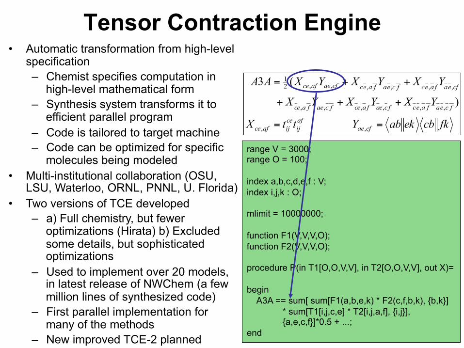
Tensor Contraction Engine

range V = 3000; range O = 100; index a,b,c,d,e,f : V; index i,j,k : O; mlimit = 10000000; function F1(V,V,V,O); function F2(V,V,V,O); procedure P(in T1[O,O,V,V], in T2[O,O,V,V], out X)= begin A3A == sum[ sum[F1(a,b,e,k) * F2(c,f,b,k), {b,k}]

* sum[T1[i,j,c,e] * T2[i,j,a,f], {i,j}], {a,e,c,f}]*0.5 + ...;

end

fkcbekabYttX

YXYXYX

YXYXYXAA

cfaeafij

ceijafce

fceafaecfceafaecfcaefaec

cfeafaecfceafaeccfaeafce

==

+++

++=

,,

,,,,,,

,,,,,,21

)

(3

•  Automatic transformation from high-level

specification –  Chemist specifies computation in

high-level mathematical form –  Synthesis system transforms it to

efficient parallel program –  Code is tailored to target machine –  Code can be optimized for specific

molecules being modeled •  Multi-institutional collaboration (OSU,

LSU, Waterloo, ORNL, PNNL, U. Florida) •  Two versions of TCE developed

–  a) Full chemistry, but fewer optimizations (Hirata) b) Excluded some details, but sophisticated optimizations

–  Used to implement over 20 models, in latest release of NWChem (a few million lines of synthesized code)

–  First parallel implementation for many of the methods

–  New improved TCE-2 planned

Domain-Specific Examples

•  Stencil computations •  Tensor expressions •  Affine computations

Why Polyhedral Compiler Optimization? •  Conven+onal  AST-­‐based  compiler  frameworks  not  powerful  enough  to  transform  imperfectly  nested  loops  effec+vely  –  Intel  icc,  PGI  pgcc,  gcc  

•  Polyhedral  model:  powerful  mathema+cal  framework  –   Transforma+on  of  affine  computa+ons  (“Sta+c  Control  Parts”)  

•  SCoPs:  loops,  condi+onals,  assignment  stmts;  array  index  exprs,  condi+onal  exprs,  loop  bound  exprs  all  affine  func+ons  of  outer  loop  iterators  

– Automa+c  paralleliza+on  and  data  locality  op+miza+on  for  (  t  =0;  t  <=T−1;t++)    {        B[1]=(A[2]+A[1]+A[0])/3;              for  (  i  =2∗t+2;  i  <=2∗t+N−2;i++)                      {    B[−2∗t+i]=(A[−2∗t+i+1]+A[−2∗t+i]+A[−2∗t+i−1])/3;                            A[−2∗t+i−1]=B[−2∗t+i−1];                      }                  A[N−2]=B[N−2];    }    

for  (  t  =0;  t  <=T−1;t++)    {            for  (  i  =  1;  i  <  N−2;i++)                      B[i]=(A[i-­‐1]+A[i]+A[i+1])/3;        for  (  i  =  1;  i  <  N−2;i++)                        A[i]=B[i];    }      

for (t = 0; t < T; t++) { for (i = 2; i < N - 1; i++) b[i]=(a[i-1]+a[i]+a[i+1])/3; for (j = 2; j < N - 1; j++) a[j] = b[j]; }

Data Dependences and Tiling

t

i

Tiling  code  as-­‐is  not  legal  due  to  cyclic  inter-­‐+le  dependences  

If  N>cachesize,  #misses:  no  +ling:  O(N*T/L)    +lesize  B:  O(N*T/(L*B))  

25  

1D-­‐Jacobi  code  

Original  execu+on  ordering  makes  +ling  Illegal  

Dependence-­‐preserving  reordering  of  itera+on  space  makes  +ling  legal  

26  

Transformation to Enable Tiling

Transformation to Enable Tiling for  (t0=0;t0<=T-­‐1;t0++)  {      b[2]=  (a[3]+a[2]+a[1])/3  ;      for  (t1=2*t0+3;t1<=2*t0+N-­‐2;t1++)  {          b[-­‐2*t0+t1]=  (a[-­‐2*t0+t1-­‐1]+                                                  a[-­‐2*t0+t1]+a[-­‐2*t0+t1+1])/3  ;          a[-­‐2*t0+t1-­‐1]=b[-­‐2*t0+t1-­‐1]  ;}      a[N-­‐2]=b[N-­‐2]  ;}  

Peeling,  skewing  and  fusion  needed  to  make  +ling  legal,  i.e.  eliminate  all  cyclic  inter-­‐+le    dependence  

t

i 27  

Polyhedral Compiler Transformation

for  (i=0;  i<N;  i++)  {      for  (j=0;  j<N;  j++)              for(k=0;  k<N;  k++)  S1;      for  (p=0;  p<M;  p++)S2;    }  

N=4  M=3  

•  Uniform,  powerful  abstrac+on  for  imperfect  loop  nests  •  Uniform,  powerful  handling  of  parametric  loop  bounds  •  Loop  transform  ==  Affine  hyperplane  schedule      =>Arbitrary  sequence  of  transforms  ==  change  of  affine  coeffs.    

Pluto Auto-Parallelizing Optimizer for(t=0;  t<tmax;  t++)    {      for  (j=0;  j<ny;  j++)          ey[0][j]  =  init_f[t];      for  (i=1;  i<nx;  i++)          for  (j=0;  j<ny;  j++)              ey[i][j]=ey[i][j]-­‐0.5*(hz[i][j]-­‐hz[i-­‐1][j]);      for  (i=0;  i<nx;  i++)          for  (j=1;  j<ny;  j++)              ex[i][j]=ex[i][j]-­‐0.5*(hz[i][j]-­‐hz[i][j-­‐1]);      for  (i=0;  i<nx;  i++)          for  (j=0;  j<ny;  j++)              hz[i][j]=hz[i][j]-­‐0.7*(ex[i][j+1]                            -­‐ex[i][j]+ey[i+1][j]-­‐ey[i][j]);  

for  (t1=0;t1<=floord(2*tmax+ny-­‐2,32);t1++)  {    lb1=max(ceild(t1,2),ceild(32*t1-­‐tmax+1,32));    ub1=min(min(floord(tmax+ny-­‐1,32),floord(32*t1+ny+31,64)),t1);  #pragma  omp  parallel  for  shared(t1,lb1,ub1)  private(t2,t3,t4,t5,t6)    for  (t2=lb1;  t2<=ub1;  t2++)  {      for  (t3=max(ceild(32*t2-­‐ny-­‐30,32),t1-­‐t2);  t3<=min(min(floord(32*t2+nx+30,32),                            floord(tmax+nx-­‐1,32)),  floord(32*t1-­‐32*t2+nx+31,32));t3++)  {                  if  ((t1  ==  t2+t3)  &&  (t1  <=  floord(64*t2-­‐ny,32)))  {                      for  (t6=32*t2-­‐ny+1;t6<=min(32*t1-­‐32*t2+31,32*t2-­‐ny+nx);t6++)  {                          hz[-­‐32*t2+t6+ny-­‐1][ny-­‐1]=hz[-­‐32*t2+t6+ny-­‐1][ny-­‐1]-­‐  0.7*(ex[-­‐32*t2+t6+ny-­‐1][ny-­‐1  +1]-­‐                              ex[-­‐32*t2+t6+ny-­‐1][ny-­‐1]+ey[-­‐32*t2+t6+ny-­‐1  +1][ny-­‐1]-­‐ey[-­‐32*t2+t6+ny-­‐1][ny-­‐1]);}}  ...  200+  lines  of  output  code  omived  ...  

Input  Sequen+al  C  Code    for  2D  FDTD  Kernel  

Output  Parallel  Tiled  C  Code  automa+cally  generated  by    Pluto  source-­‐source  op+mizer  

30

Center for Domain-Specific Computing Supported by NSF “Expedition in Computing” Program

www.cdsc.ucla.edu.

Jason Cong

CDSC Director

31

Center for Domain-Specific Computing

UCLA Rice UCSB Ohio State

Domain-specific modeling Bui, Reinman, Potkonjak Sarkar, Baraniuk Sadayappan

CHP creation Chang, Cong, Reinman Cheng

CHP mapping Cong, Palsberg, Potkonjak Sarkar � Cheng � Sadayappan �

Application modeling Aberle, Bui, Chien, Vese Baraniuk �

Experimental systems All All All � All �

Reinman Palsberg Sadayappan Sarkar (Associate Dir)

Vese Potkonjak

Aberle Baraniuk Bui Cong (Director) Cheng Chang

A diverse inter-disciplinary team: 8 in CS&E; 1 in EE; 3 in medical school; 1 in applied math

Chien

32

- Current solution: Parallelization - Next Significant Opportunity -- Customization

Parallelization

Source: Shekhar Borkar, Intel

Customization

Adapt architecture to application domain

New Transformative Approach to Power/Energy Efficient Computing

33

 [1] Amphion CS5230 on Virtex2 + Xilinx Virtex2 Power Estimator

 [2] Dag Arne Osvik: 544 cycles AES – ECB on StrongArm SA-1110

 [3] Helger Lipmaa PIII assembly handcoded + Intel Pentium III (1.13 GHz) Datasheet

 [4] gcc, 1 mW/MHz @ 120 Mhz Sparc – assumes 0.25 u CMOS

 [5] Java on KVM (Sun J2ME, non-JIT) on 1 mW/MHz @ 120 MHz Sparc – assumes 0.25 u CMOS

Potential of Customization

648 Mbits/sec Asm

Pentium III [3] 41.4 W 0.015 (1/800)

Java [5] Emb. Sparc 450 bits/sec 120 mW

0.0000037 (1/3,000,000)

C Emb. Sparc [4] 133 Kbits/sec 0.0011 (1/10,000)

350 mW

 Power

1.32 Gbit/sec FPGA [1]

11 (1/1) Ø 3.84 Gbits/sec 0.18µm CMOS

 Figure of Merit (Gb/s/W)

 Throughput  AES 128bit key 128bit data

490 mW 2.7 (1/4)

120 mW

ASM StrongARM [2] 240 mW 0.13 (1/85) 31 Mbit/sec

Source: P. Schaumont, and I. Verbauwhede, "Domain specific codesign for embedded security," IEEE Computer 36(4), 2003.

34

Advance of Civilization

  For human brain, Moore’s Law scaling has long stopped §  The number neurons and their firing speed did not change significantly

 Remarkable advancement of civilization via specialization   More advanced societies have higher degree of specialization

35

CDSC Project Goals

 A customizable platform for the given domain(s) § Can be customized to a wide-range of applications in

the domain § Can be massively produced with cost efficiency § Can be programmed efficiently with novel compilation

and runtime systems

 Metric of success § A “supercomputer-in-a-box” with 100X performance/

power improvement via customization for the intended domain(s)

36

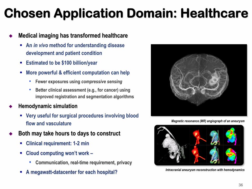
Chosen Application Domain: Healthcare

  Medical imaging has transformed healthcare §  An in vivo method for understanding disease

development and patient condition §  Estimated to be $100 billion/year §  More powerful & efficient computation can help

•  Fewer exposures using compressive sensing •  Better clinical assessment (e.g., for cancer) using

improved registration and segmentation algorithms

  Hemodynamic simulation §  Very useful for surgical procedures involving blood

flow and vasculature

  Both may take hours to days to construct §  Clinical requirement: 1-2 min §  Cloud computing won’t work –

•  Communication, real-time requirement, privacy

§  A megawatt-datacenter for each hospital?

Intracranial aneurysm reconstruction with hemodynamics

Magnetic resonance (MR) angiograph of an aneurysm

37

Customizable Heterogeneous Platform (CHP)

$ $ $ $

Fixed Core

Fixed Core

Fixed Core

Fixed Core

Custom Core

Custom Core

Custom Core

Custom Core

Prog Fabric

Prog Fabric accelerator accelerator

DRAM

DRAM

I/O

CHP

CHP

CHP

Reconfigurable RF-I bus Reconfigurable optical bus

Transceiver/receiver Optical interface

Overview of CDSC Research Program

CHP mapping Source-to-source CHP mapper

Reconfiguring & optimizing backend Adaptive runtime

Domain-specific-modeling (healthcare applications)

CHP creation Customizable computing engines

Customizable interconnects

Architecture modeling

Customization setting Design once Invoke many times

Summary

•  The  `power  wall’  has  made  heterogeneous  compu+ng  essen+al  

•  Heterogeneous  compu+ng  creates  huge  soTware  challenges  

•  Domain-­‐specific  compu+ng  is  a  promising  approach  to  effec+ve  heterogeneous  compu+ng  – Produc+vity,  portability,  performance  – Write  once,  execute  anywhere  

•  Close  interac+on  between  domain  experts,  systems  soTware  experts,  and  architects  will  be  essen+al