p hi ts · preface this manual is the particle and heavy ion transport code system (phits) user’s...
TRANSCRIPT

English version
PHITS
Ver. 3.02 User’s Manual

Preface
This manual is the Particle and Heavy Ion Transport code System (PHITS) user’s guide. PHITS is a general-purpose Monte Carlo particle transport simulation code that is used in many studies in the fields of acceleratortechnology, radiotherapy, space radiation, etc. For details on the physical models and important functions imple-mented in PHITS, see the main article1, benchmark study2, and papers citing them. This manual explains how toexecute PHITS and which parameters should be used in the system.
The contents of this manual correspond to the PHITS version number shown on the title page and are subjectto change without notice. If you have any question or comment regarding this manual, please contact the PHITSoffice ([email protected]).
1 T. Sato, K. Niita, N. Matsuda, S. Hashimoto, Y. Iwamoto, S. Noda, T. Ogawa, H. Iwase, H. Nakashima, T. Fukahori, K. Okumura, T. Kai,S. Chiba, T. Furuta, and L. Sihver, Particle and Heavy Ion Transport Code System PHITS, Version 2.52, J. Nucl. Sci. Technol. 50:9, 913-923(2013).
2 Y. Iwamoto, T. Sato, S. Hashimoto, T. Ogawa, T. Furuta, S. Abe, T. Kai, N. Matsuda, R. Hosoyamada, and K. Niita, Benchmark study ofthe recent version of the PHITS code, J. Nucl. Sci. Technol. 54:5, 617-635 (2017).
I

Contents
1 Recent Improvements and Development members 11.1 Recent Improvements. . . . . . . . . . . . . . . . . . . . . . . . . . . . . . . . . . . . . . . . . 11.2 Development members. . . . . . . . . . . . . . . . . . . . . . . . . . . . . . . . . . . . . . . . 121.3 Reference of PHITS. . . . . . . . . . . . . . . . . . . . . . . . . . . . . . . . . . . . . . . . . .12
2 Installation, compilation and execution of PHITS 142.1 Operating environment. . . . . . . . . . . . . . . . . . . . . . . . . . . . . . . . . . . . . . . . 142.2 Installation and execution on Windows. . . . . . . . . . . . . . . . . . . . . . . . . . . . . . . . 142.3 Installation and execution on Mac. . . . . . . . . . . . . . . . . . . . . . . . . . . . . . . . . . 152.4 Compilation using “make”command for Windows, Mac, and Linux. . . . . . . . . . . . . . . . 182.5 Compilation using Microsoft Visual Studio with Intel Fortran for Windows. . . . . . . . . . . . 192.6 Compilation of ANGEL . . . . . . . . . . . . . . . . . . . . . . . . . . . . . . . . . . . . . . . 202.7 Executable file . . . . . . . . . . . . . . . . . . . . . . . . . . . . . . . . . . . . . . . . . . . .202.8 Terminating the PHITS code. . . . . . . . . . . . . . . . . . . . . . . . . . . . . . . . . . . . . 202.9 Array sizes . . . . . . . . . . . . . . . . . . . . . . . . . . . . . . . . . . . . . . . . . . . . . .21
3 Input File 223.1 Sections. . . . . . . . . . . . . . . . . . . . . . . . . . . . . . . . . . . . . . . . . . . . . . . .223.2 Reading control. . . . . . . . . . . . . . . . . . . . . . . . . . . . . . . . . . . . . . . . . . . .233.3 Inserting files . . . . . . . . . . . . . . . . . . . . . . . . . . . . . . . . . . . . . . . . . . . . .243.4 User-defined variables. . . . . . . . . . . . . . . . . . . . . . . . . . . . . . . . . . . . . . . . 243.5 Using mathematical expressions. . . . . . . . . . . . . . . . . . . . . . . . . . . . . . . . . . . 253.6 Particle identification. . . . . . . . . . . . . . . . . . . . . . . . . . . . . . . . . . . . . . . . . 26
4 Sections format 284.1 [ Title ] section . . . . . . . . . . . . . . . . . . . . . . . . . . . . . . . . . . . . . . . . . . . .284.2 [ Parameters ] section. . . . . . . . . . . . . . . . . . . . . . . . . . . . . . . . . . . . . . . . . 29
4.2.1 Calculation mode. . . . . . . . . . . . . . . . . . . . . . . . . . . . . . . . . . . . . . . 294.2.2 Number of history and Bank. . . . . . . . . . . . . . . . . . . . . . . . . . . . . . . . . 304.2.3 Cut-off energy and switching energy. . . . . . . . . . . . . . . . . . . . . . . . . . . . . 324.2.4 Cut-off time, cut-off weight, and weight window . . . . . . . . . . . . . . . . . . . . . . 354.2.5 Model option (1) . . . . . . . . . . . . . . . . . . . . . . . . . . . . . . . . . . . . . . . 364.2.6 Model option (2) . . . . . . . . . . . . . . . . . . . . . . . . . . . . . . . . . . . . . . . 374.2.7 Model option (3) . . . . . . . . . . . . . . . . . . . . . . . . . . . . . . . . . . . . . . . 384.2.8 Model option (4) . . . . . . . . . . . . . . . . . . . . . . . . . . . . . . . . . . . . . . . 394.2.9 Model option (5) . . . . . . . . . . . . . . . . . . . . . . . . . . . . . . . . . . . . . . . 404.2.10 Output options (1). . . . . . . . . . . . . . . . . . . . . . . . . . . . . . . . . . . . . . 404.2.11 Output options (2). . . . . . . . . . . . . . . . . . . . . . . . . . . . . . . . . . . . . . 434.2.12 Output option (3). . . . . . . . . . . . . . . . . . . . . . . . . . . . . . . . . . . . . . . 444.2.13 Output option (4). . . . . . . . . . . . . . . . . . . . . . . . . . . . . . . . . . . . . . . 454.2.14 Output option (5). . . . . . . . . . . . . . . . . . . . . . . . . . . . . . . . . . . . . . . 464.2.15 About geometrical errors. . . . . . . . . . . . . . . . . . . . . . . . . . . . . . . . . . . 474.2.16 Input-output file name. . . . . . . . . . . . . . . . . . . . . . . . . . . . . . . . . . . . 484.2.17 Others. . . . . . . . . . . . . . . . . . . . . . . . . . . . . . . . . . . . . . . . . . . . .494.2.18 Physical parameters for low energy neutrons. . . . . . . . . . . . . . . . . . . . . . . . 494.2.19 Physical parameters for photon and electron transport based on the original model. . . . 504.2.20 Parameters for EGS5. . . . . . . . . . . . . . . . . . . . . . . . . . . . . . . . . . . . . 514.2.21 Dumpall option. . . . . . . . . . . . . . . . . . . . . . . . . . . . . . . . . . . . . . . . 544.2.22 Event Generator Mode. . . . . . . . . . . . . . . . . . . . . . . . . . . . . . . . . . . . 58
4.3 [ Source ] section. . . . . . . . . . . . . . . . . . . . . . . . . . . . . . . . . . . . . . . . . . .594.3.1 <Source> : Multi-source . . . . . . . . . . . . . . . . . . . . . . . . . . . . . . . . . . . 604.3.2 Common parameters. . . . . . . . . . . . . . . . . . . . . . . . . . . . . . . . . . . . . 614.3.3 Cylinder distribution source. . . . . . . . . . . . . . . . . . . . . . . . . . . . . . . . . 634.3.4 Rectangular solid distribution source. . . . . . . . . . . . . . . . . . . . . . . . . . . . . 634.3.5 Gaussian distribution source (x,y,z independent). . . . . . . . . . . . . . . . . . . . . . 64
ii

4.3.6 Generic parabola distribution source (x,y,z independent). . . . . . . . . . . . . . . . . . 644.3.7 Gaussian distribution source (x-y plane). . . . . . . . . . . . . . . . . . . . . . . . . . . 654.3.8 Generic parabola distribution source (x-y plane). . . . . . . . . . . . . . . . . . . . . . . 654.3.9 Sphere and spherical shell distribution source. . . . . . . . . . . . . . . . . . . . . . . . 664.3.10 s-type= 11 . . . . . . . . . . . . . . . . . . . . . . . . . . . . . . . . . . . . . . . . . .674.3.11 s-type= 12 . . . . . . . . . . . . . . . . . . . . . . . . . . . . . . . . . . . . . . . . . .674.3.12 Cone shape. . . . . . . . . . . . . . . . . . . . . . . . . . . . . . . . . . . . . . . . . .684.3.13 Triangle prism shape. . . . . . . . . . . . . . . . . . . . . . . . . . . . . . . . . . . . . 694.3.14 xyz-mesh distribution source. . . . . . . . . . . . . . . . . . . . . . . . . . . . . . . . . 704.3.15 Reading dump file. . . . . . . . . . . . . . . . . . . . . . . . . . . . . . . . . . . . . . 724.3.16 User definition source. . . . . . . . . . . . . . . . . . . . . . . . . . . . . . . . . . . . 754.3.17 Definitions for energy distribution. . . . . . . . . . . . . . . . . . . . . . . . . . . . . . 784.3.18 Definition for angular distribution. . . . . . . . . . . . . . . . . . . . . . . . . . . . . . 904.3.19 Definition for time distribution. . . . . . . . . . . . . . . . . . . . . . . . . . . . . . . . 924.3.20 Example of multi-source. . . . . . . . . . . . . . . . . . . . . . . . . . . . . . . . . . . 944.3.21 Duct source option. . . . . . . . . . . . . . . . . . . . . . . . . . . . . . . . . . . . . . 98
4.4 [ Material ] section . . . . . . . . . . . . . . . . . . . . . . . . . . . . . . . . . . . . . . . . . .1014.4.1 Formats. . . . . . . . . . . . . . . . . . . . . . . . . . . . . . . . . . . . . . . . . . . .1014.4.2 Element (nuclide) definition. . . . . . . . . . . . . . . . . . . . . . . . . . . . . . . . .1014.4.3 Composition ratio definition. . . . . . . . . . . . . . . . . . . . . . . . . . . . . . . . .1014.4.4 Material parameters. . . . . . . . . . . . . . . . . . . . . . . . . . . . . . . . . . . . .1024.4.5 S(α, β) settings . . . . . . . . . . . . . . . . . . . . . . . . . . . . . . . . . . . . . . . .1024.4.6 Examples. . . . . . . . . . . . . . . . . . . . . . . . . . . . . . . . . . . . . . . . . . .103
4.5 [ Surface ] section. . . . . . . . . . . . . . . . . . . . . . . . . . . . . . . . . . . . . . . . . . .1044.5.1 Formats. . . . . . . . . . . . . . . . . . . . . . . . . . . . . . . . . . . . . . . . . . . .1044.5.2 Examples. . . . . . . . . . . . . . . . . . . . . . . . . . . . . . . . . . . . . . . . . . .1074.5.3 Surface Definition by Macro Body. . . . . . . . . . . . . . . . . . . . . . . . . . . . . .117
4.6 [ Cell ] section. . . . . . . . . . . . . . . . . . . . . . . . . . . . . . . . . . . . . . . . . . . . .1184.6.1 Formats. . . . . . . . . . . . . . . . . . . . . . . . . . . . . . . . . . . . . . . . . . . .1184.6.2 Description of cell definition. . . . . . . . . . . . . . . . . . . . . . . . . . . . . . . . .1194.6.3 Universe frame. . . . . . . . . . . . . . . . . . . . . . . . . . . . . . . . . . . . . . . .1224.6.4 Lattice definition. . . . . . . . . . . . . . . . . . . . . . . . . . . . . . . . . . . . . . .1234.6.5 Repeated structures. . . . . . . . . . . . . . . . . . . . . . . . . . . . . . . . . . . . . .125
4.7 [ Transform ] section. . . . . . . . . . . . . . . . . . . . . . . . . . . . . . . . . . . . . . . . .1324.7.1 Formats. . . . . . . . . . . . . . . . . . . . . . . . . . . . . . . . . . . . . . . . . . . .1324.7.2 Mathematical definition of the transform. . . . . . . . . . . . . . . . . . . . . . . . . .1324.7.3 Examples (1). . . . . . . . . . . . . . . . . . . . . . . . . . . . . . . . . . . . . . . . .1334.7.4 Examples (2). . . . . . . . . . . . . . . . . . . . . . . . . . . . . . . . . . . . . . . . .133
4.8 [ Temperature ] section. . . . . . . . . . . . . . . . . . . . . . . . . . . . . . . . . . . . . . . .1344.9 [ Mat Time Change ] section. . . . . . . . . . . . . . . . . . . . . . . . . . . . . . . . . . . . .1354.10 [ Magnetic Field ] section. . . . . . . . . . . . . . . . . . . . . . . . . . . . . . . . . . . . . . .136
4.10.1 Charged particle. . . . . . . . . . . . . . . . . . . . . . . . . . . . . . . . . . . . . . .1364.10.2 Neutron. . . . . . . . . . . . . . . . . . . . . . . . . . . . . . . . . . . . . . . . . . . .137
4.11 [ Electro Magnetic Field ] section. . . . . . . . . . . . . . . . . . . . . . . . . . . . . . . . . .1384.12 [ Delta Ray ] section . . . . . . . . . . . . . . . . . . . . . . . . . . . . . . . . . . . . . . . . .1394.13 [ Track Structure ] section. . . . . . . . . . . . . . . . . . . . . . . . . . . . . . . . . . . . . .1404.14 [ Super Mirror ] section. . . . . . . . . . . . . . . . . . . . . . . . . . . . . . . . . . . . . . . .1414.15 [ Elastic Option ] section. . . . . . . . . . . . . . . . . . . . . . . . . . . . . . . . . . . . . . .1424.16 [ Data Max ] section . . . . . . . . . . . . . . . . . . . . . . . . . . . . . . . . . . . . . . . . .1434.17 [ Frag Data ] section. . . . . . . . . . . . . . . . . . . . . . . . . . . . . . . . . . . . . . . . .1444.18 [ Importance ] section. . . . . . . . . . . . . . . . . . . . . . . . . . . . . . . . . . . . . . . . .1474.19 [ Weight Window ] section. . . . . . . . . . . . . . . . . . . . . . . . . . . . . . . . . . . . . .1484.20 [ WW Bias ] section. . . . . . . . . . . . . . . . . . . . . . . . . . . . . . . . . . . . . . . . . .1494.21 [ Forced Collisions ] section. . . . . . . . . . . . . . . . . . . . . . . . . . . . . . . . . . . . .1524.22 [ Volume ] section. . . . . . . . . . . . . . . . . . . . . . . . . . . . . . . . . . . . . . . . . . .1534.23 [ Multiplier ] section . . . . . . . . . . . . . . . . . . . . . . . . . . . . . . . . . . . . . . . . .1544.24 [ Mat Name Color ] section. . . . . . . . . . . . . . . . . . . . . . . . . . . . . . . . . . . . . .155
iii

4.25 [ Reg Name ] section. . . . . . . . . . . . . . . . . . . . . . . . . . . . . . . . . . . . . . . . .1574.26 [ Counter ] section . . . . . . . . . . . . . . . . . . . . . . . . . . . . . . . . . . . . . . . . . .1584.27 [ Timer ] section. . . . . . . . . . . . . . . . . . . . . . . . . . . . . . . . . . . . . . . . . . . .160
5 Common parameters for tallies 1615.1 Geometrical mesh. . . . . . . . . . . . . . . . . . . . . . . . . . . . . . . . . . . . . . . . . . .161
5.1.1 Region mesh. . . . . . . . . . . . . . . . . . . . . . . . . . . . . . . . . . . . . . . . .1615.1.2 Definition of the region and volume for repeated structures and lattices. . . . . . . . . . 1625.1.3 r-z mesh. . . . . . . . . . . . . . . . . . . . . . . . . . . . . . . . . . . . . . . . . . . .1635.1.4 xyz mesh. . . . . . . . . . . . . . . . . . . . . . . . . . . . . . . . . . . . . . . . . . .164
5.2 Energy mesh . . . . . . . . . . . . . . . . . . . . . . . . . . . . . . . . . . . . . . . . . . . . .1645.3 LET mesh. . . . . . . . . . . . . . . . . . . . . . . . . . . . . . . . . . . . . . . . . . . . . . .1645.4 Time mesh. . . . . . . . . . . . . . . . . . . . . . . . . . . . . . . . . . . . . . . . . . . . . . .1655.5 Angle mesh. . . . . . . . . . . . . . . . . . . . . . . . . . . . . . . . . . . . . . . . . . . . . .1655.6 Mesh definition. . . . . . . . . . . . . . . . . . . . . . . . . . . . . . . . . . . . . . . . . . . .165
5.6.1 Mesh type. . . . . . . . . . . . . . . . . . . . . . . . . . . . . . . . . . . . . . . . . . .1655.6.2 e-type= 1 . . . . . . . . . . . . . . . . . . . . . . . . . . . . . . . . . . . . . . . . . . .1655.6.3 e-type= 2, 3 . . . . . . . . . . . . . . . . . . . . . . . . . . . . . . . . . . . . . . . . .1675.6.4 e-type= 4 . . . . . . . . . . . . . . . . . . . . . . . . . . . . . . . . . . . . . . . . . . .1675.6.5 e-type= 5 . . . . . . . . . . . . . . . . . . . . . . . . . . . . . . . . . . . . . . . . . . .167
5.7 Other tally definitions. . . . . . . . . . . . . . . . . . . . . . . . . . . . . . . . . . . . . . . . .1675.7.1 Particle definition. . . . . . . . . . . . . . . . . . . . . . . . . . . . . . . . . . . . . . .1675.7.2 axis definition. . . . . . . . . . . . . . . . . . . . . . . . . . . . . . . . . . . . . . . . .1685.7.3 file definition . . . . . . . . . . . . . . . . . . . . . . . . . . . . . . . . . . . . . . . . .1695.7.4 resfile definition . . . . . . . . . . . . . . . . . . . . . . . . . . . . . . . . . . . . . . .1695.7.5 unit definition. . . . . . . . . . . . . . . . . . . . . . . . . . . . . . . . . . . . . . . . .1695.7.6 factor definition. . . . . . . . . . . . . . . . . . . . . . . . . . . . . . . . . . . . . . . .1705.7.7 output definition . . . . . . . . . . . . . . . . . . . . . . . . . . . . . . . . . . . . . . .1705.7.8 info definition. . . . . . . . . . . . . . . . . . . . . . . . . . . . . . . . . . . . . . . . .1705.7.9 title definition. . . . . . . . . . . . . . . . . . . . . . . . . . . . . . . . . . . . . . . . .1705.7.10 ANGEL parameter definition. . . . . . . . . . . . . . . . . . . . . . . . . . . . . . . . .1705.7.11 SANGEL parameter definition. . . . . . . . . . . . . . . . . . . . . . . . . . . . . . . .1715.7.12 2d-type definition. . . . . . . . . . . . . . . . . . . . . . . . . . . . . . . . . . . . . . .1715.7.13 gshow definition. . . . . . . . . . . . . . . . . . . . . . . . . . . . . . . . . . . . . . .1725.7.14 rshow definition . . . . . . . . . . . . . . . . . . . . . . . . . . . . . . . . . . . . . . .1725.7.15 x-txt, y-txt, z-txt definition. . . . . . . . . . . . . . . . . . . . . . . . . . . . . . . . . .1735.7.16 volmat definition. . . . . . . . . . . . . . . . . . . . . . . . . . . . . . . . . . . . . . .1735.7.17 epsout definition. . . . . . . . . . . . . . . . . . . . . . . . . . . . . . . . . . . . . . .1735.7.18 counter definition. . . . . . . . . . . . . . . . . . . . . . . . . . . . . . . . . . . . . . .1745.7.19 resolution and line thickness definitions. . . . . . . . . . . . . . . . . . . . . . . . . . .1745.7.20 trcl coordinate transformation. . . . . . . . . . . . . . . . . . . . . . . . . . . . . . . .1745.7.21 dump definition. . . . . . . . . . . . . . . . . . . . . . . . . . . . . . . . . . . . . . . .174
5.8 Function to sum up two (or more) tally results. . . . . . . . . . . . . . . . . . . . . . . . . . . .176
6 Tally input format 1786.1 [ T-Track ] section. . . . . . . . . . . . . . . . . . . . . . . . . . . . . . . . . . . . . . . . . . .1786.2 [ T-Cross ] section. . . . . . . . . . . . . . . . . . . . . . . . . . . . . . . . . . . . . . . . . . .1826.3 [ T-Point ] section. . . . . . . . . . . . . . . . . . . . . . . . . . . . . . . . . . . . . . . . . . .1886.4 [ T-Heat ] section . . . . . . . . . . . . . . . . . . . . . . . . . . . . . . . . . . . . . . . . . . .1916.5 [ T-Deposit ] section . . . . . . . . . . . . . . . . . . . . . . . . . . . . . . . . . . . . . . . . .1946.6 [ T-Deposit2 ] section. . . . . . . . . . . . . . . . . . . . . . . . . . . . . . . . . . . . . . . . .1996.7 [ T-Yield ] section. . . . . . . . . . . . . . . . . . . . . . . . . . . . . . . . . . . . . . . . . . .2016.8 [ T-Product ] section . . . . . . . . . . . . . . . . . . . . . . . . . . . . . . . . . . . . . . . . .2046.9 [ T-DPA ] section . . . . . . . . . . . . . . . . . . . . . . . . . . . . . . . . . . . . . . . . . . .2086.10 [ T-LET ] section . . . . . . . . . . . . . . . . . . . . . . . . . . . . . . . . . . . . . . . . . . .2116.11 [ T-SED ] section . . . . . . . . . . . . . . . . . . . . . . . . . . . . . . . . . . . . . . . . . . .2146.12 [ T-Time ] section. . . . . . . . . . . . . . . . . . . . . . . . . . . . . . . . . . . . . . . . . . .217
iv

6.13 [ T-Star ] section . . . . . . . . . . . . . . . . . . . . . . . . . . . . . . . . . . . . . . . . . . .2206.14 [ T-Dchain ] section . . . . . . . . . . . . . . . . . . . . . . . . . . . . . . . . . . . . . . . . .2236.15 [ T-WWG ] section . . . . . . . . . . . . . . . . . . . . . . . . . . . . . . . . . . . . . . . . . .2276.16 [ T-WWBG ] section . . . . . . . . . . . . . . . . . . . . . . . . . . . . . . . . . . . . . . . . .2296.17 [ T-Volume ] section. . . . . . . . . . . . . . . . . . . . . . . . . . . . . . . . . . . . . . . . . .2326.18 [ T-Userdefined ] section. . . . . . . . . . . . . . . . . . . . . . . . . . . . . . . . . . . . . . .2336.19 [ T-Gshow ] section. . . . . . . . . . . . . . . . . . . . . . . . . . . . . . . . . . . . . . . . . .2376.20 [ T-Rshow ] section. . . . . . . . . . . . . . . . . . . . . . . . . . . . . . . . . . . . . . . . . .2396.21 [ T-3Dshow ] section. . . . . . . . . . . . . . . . . . . . . . . . . . . . . . . . . . . . . . . . .241
6.21.1 box definition. . . . . . . . . . . . . . . . . . . . . . . . . . . . . . . . . . . . . . . . .2446.21.2 3dshow example. . . . . . . . . . . . . . . . . . . . . . . . . . . . . . . . . . . . . . .245
7 Automatic calculation of region volume 248
8 Processing dump file 249
9 Output cutoff data format 253
10 Region error check 254
11 Additional explanation for parallel computing 25511.1 Distributed memory parallel computing. . . . . . . . . . . . . . . . . . . . . . . . . . . . . . .255
11.1.1 Execution. . . . . . . . . . . . . . . . . . . . . . . . . . . . . . . . . . . . . . . . . . .25511.1.2 Adjustment of maxcas and maxbch. . . . . . . . . . . . . . . . . . . . . . . . . . . . .25511.1.3 Treatment of abnormal ending. . . . . . . . . . . . . . . . . . . . . . . . . . . . . . . .25511.1.4 ncut, gcut, pcut, and dumpall file definition in PHITS. . . . . . . . . . . . . . . . . . . . 25611.1.5 Read-in file definition in PHITS. . . . . . . . . . . . . . . . . . . . . . . . . . . . . . .256
11.2 Shared-memory parallel computing. . . . . . . . . . . . . . . . . . . . . . . . . . . . . . . . .25611.2.1 Execution. . . . . . . . . . . . . . . . . . . . . . . . . . . . . . . . . . . . . . . . . . .25611.2.2 Important notices for shared-memory parallel computing. . . . . . . . . . . . . . . . . . 257
12 FAQ 25812.1 Questions related to parameter setting. . . . . . . . . . . . . . . . . . . . . . . . . . . . . . . .25812.2 Questions related to error occurred in compiling or executing PHITS. . . . . . . . . . . . . . . . 25912.3 Questions related to Tally. . . . . . . . . . . . . . . . . . . . . . . . . . . . . . . . . . . . . . .26012.4 Questions related to source generation. . . . . . . . . . . . . . . . . . . . . . . . . . . . . . . .261
index 262
v

1
1 Recent Improvements and Development members
1.1 Recent Improvements
Essences of improvements after version 2.24 are described below.
From ver. 3.02, the following functions were implemented, and some bugs were fixed. (2017/12/01)
• New parametersnudtvar andudtvar(i) were introduced for[t-userdefined]. After variablesudtvar(i),(i = 1, · · · , nudtvar) was set in an input file, these can be used insubroutine usrtally. There is noupper limit of the number ofudtvar(i) unlikeudtpara before ver. 3.01.udtpara can be also set after thisversion.
• New options were implemented for theunit of [t-let] and[t-sed].
• Position of the source generation was adjusted to just on the spherical surface fors-type=9 with dir=iso.This revision influences only when some materials are placed outside the source sphere.
• A bug related to[counter] section was revised. Before this revision, occurrence of atomic interactionswere ignored in calculating counter whennegs was set to-1 (only photon transport mode).
• A bug in the calculation of the restricted stopping power when delta-rays are generated by[delta ray]
was fixed.
• The bug in the calculation of angular straggling usingnspred = 2 was fixed. This bug was introducedin PHITS2.96, and calculation results for charged particle beam using the versions between 2.96 and 3.01might be strange.
From ver. 3.01, the following functions were implemented, and some bugs were fixed. (2017/10/31)
• A special ANGEL parametersangel was introduced to insert all ANGEL parameters into tally outputfiles. This function was developed by Mr. Takamitsu Miura of RIST, and was supported by Center forComputational Science & e-Systems, JAEA.
• Reading algorithm for tetrahedral geometry was revised to reduce the computational time.
• ANGEL was revised to reduce the computational time for makingeps files of tally results with 2-dimensionaltype such asaxis=xy.
• A bug for ignoringstdcut in [t-deposit] was fixed.
From ver. 3.00, the Kurotama model was used as the default model to give nucleus-nucleus reaction crosssections, and the natural isotope expansion was effective in input files of DCHAIN-SP generated by[t-dchain].In addition, some bugs were fixed. (2017/10/04)
From ver. 2.97, the following functions were implemented, and some bugs were fixed. (2017/09/21)
• A new parameteriMeVperu was introduced to convert the unit of nucleus energy [MeV] to [MeV/u] inoutputs of all tallies. By setting ofiMeVperu=1 in [parameters], all tally results are output with the unitof MeV/u for the nucleus energy. This function was developed by Mr. Takamitsu Miura of RIST, and wassupported by Center for Computational Science & e-Systems, JAEA.
• New parametersr-from, r-to in [t-cross] with mesh=reg were added, because conventional parame-tersr-in, r-out were confusing.r-from, r-to can be used instead ofr-in, r-out, respectively.
• The option of the stopping powerndedx=3 became applicable for target nuclei with the mass number of93≤ Z ≤ 97 (from Np to Bk). See Section4.2.8for more detail.
• By adding “$OMP=N” (N is the number of CPU cores to be used) before the first section in a PHITS inputfile, the shared-memory parallel computing using OpenMP is executed. Even wheninfl: is set, a line of“file=input file name” is not required. In Mac OS, a terminal window is opened when PHITS is executedby drag and drop on the Dock. Note that these function are not available when to run PHITS on the commandline on Linux and so on.

2 1 RECENT IMPROVEMENTS AND DEVELOPMENT MEMBERS
• The default value of the switching energy from JQMD to JAMQMD,ejamqmd, was changed to 3GeV.
From ver. 2.96, the following functions were implemented, and some bugs were fixed. (2017/08/28)
• A new section[ww bias] and a new tally[t-wwbg] were implemented to bias[weight window] toobtain better statistics for a certain direction. See Section4.20and6.16in more detail.
• The numerical data of tally results are outputted after each batch is finished even foritall=0 (default).Thus, the difference betweenitall=1 and 0 is whether the image (*.eps) files are generated or not. Owingto this revision, the parameterstdcut works in the default setting.
• Only related tallies to the setting of theicntl parameter work. For example, all tallies except for[t-volume]are disabled whenicntl=14, while [t-volume] is disabled whenicntl,14. Warning is outputted wheninfl or set command is written in the disabled section.
• Some ANGEL parameters were introduced to change the length or time axis of figures. For example, youcan draw a figure of spatial dose distribution with the axis in nm scale by settingangel=cmnm in the tally.See section5.7.10in more detail.
• PHITS execution is terminated when two or more[parameters] sections exist in one input file.
• Some bugs are fixed in terms of the systematic equation for calculating the giant-dipole resonance cross sec-tions, the angular straggling function for very short range particle, high-energy nucleon-nucleon interactionmodel JAMQMD2, and the formula for calculating the source spectrum with the Maxwell distribution.
From ver. 2.95, the procedure fors-type depending on the setting of the energy of source particles waschanged. The mono-energetic and energy-distributed sources can be defined by settinge0 ande-type, respec-tively, irrespective of the value ofs-type. If both e0 ande-type are defined, the energy is decided according tothe previous procedure ofs-type. In addition, some bugs were fixed. (2017/07/21)
From ver. 2.94, bug in[t-track] and[t-cross] was fixed. Before this revision, the energy of electrons andpositrons passing through vacuum is slightly different from the real value when EGS5 mode is used. Note that thisrevision only influences the tally results, and has no relation with particle transport simulation itself. In addition,bugs in track-structure mode were fixed. (2017/06/30)
From version 2.93, the following functions were implemented, and some bugs were fixed. (2017/06/16)
• A new parameterfile(1)was introduced to specify the PHITS installation folder name. When you properlyset this parameter, you do not have to specify the name of other input files i.e.file(7, 20, 21, 24, and
25) unless you have changed the folder structure of PHITS.
• A new parameternucdata was introduced to automatically adjustemin(2) anddmax(2) parameters suit-able for JENDL-4.0. The default value of this parameter is set to 1, i.e. neutrons below 20 MeV areautomatically transported using nuclear data library.
• A new option fornegs parameter, -1, was introduced. When you setnegs = -1, PHITS treats photontransport using the original algorithm (i.e. not EGS5), and ignores the electron and positron transport. Thisoption is selected as the default setting.
• The default value ofides parameter was changed to 1, i.e. photon does not produce electrons in the PHITSoriginal algorithm. If you would like to transport electrons and positrons, you have to use EGS5.
• The default value ofigamma parameter was changed to 2, i.e.γ-rays are produced in the de-excitationprocess based on EBITEM model in the default setting.
• RI source function was improved to be applicable toα andβ decays including Auger electron production.See Table4.53in more detail.
• Track-structure mode was developed in PHITS. Using this mode, PHITS can analyze ionization, excitation,and oscillation induced by electrons and positrons event-by-event. See Section4.13in more detail.
1.1 Recent Improvements 3
• A new method for calculating the energy loss of charged particles with explicitly generatingδ-rays wasdeveloped, based on their restricted stopping power. This method is selected as the default setting, i.e.irlet = 1.
• JAMQMD, which is used for simulating nucleus-nucleus interactions above 3 GeV/u, was improved toconsider the relativistic effect.
• [t-dpa] was improved to be capable of calculating DPA by electrons, positrons, pions etc.
• Bug in the normalization process of the self-fission source (ispfs option) was fixed.
From ver. 2.92, the default setting ofoutput in [t-dchain] tally changed tocutoff in order to scoreparticles stopped in specified regions. Note that in the previous settingoutput=product heavy ions producedin a thin target were scored even though the ions don’t stop in the target. In addition, we replaced a place wherethe version of PHITS is shown in eps files by that of ANGEL. We fixed a bug about triangle prism shape source.(2017/04/18)
From version 2.91, a following function was implemented, and some bugs were fixed. (2017/02/20)
• A new function to display error bars of statistical uncertainties in eps files of tally results was implemented.This function is available by settingepsout=2 in each tally section. It should be noted that the setting isignored when the output format is 2-dimensional type such asaxis=xy.
• A bug in the combination of EGS5 and[t-cross] was fixed. This bug affected calculations in whichelectrons or positrons were scored with[t-cross] using EGS5.
From version 2.90, following functions were implemented. (2017/02/09)
• A new function to analyze the motion of electrons and positrons in the electro-magnetic fields was imple-mented. This implementation was performed under support of NAIS Inc.
• The default value of theascat2 parameter introduced in version 2.77 was revised from 0.088 to 0.038, inaccordance with the original paper3. The PHITS results obtained by settingnspred = 2without specifyingascat2 will be changed.
• A new function to generate xyz-mesh distribution source was implemented. Using this function, you canreproduce sources having a complex spatial distribution. See Section4.3.14in more detail.
• A new tally named[t-volume] was developed in order to automatically calculate the volume of each cell.See Sections6.17and7 in more detail.
• A new parametertimeout was introduced in the[parameters] section. When CPU time exceeds thisvalue, the PHITS simulation is automatically stopped. This check function works at the end of each batch.
• A new parameterstdcut was introduced in each tally. When the all statistical uncertainties of the tallyresults become less than this value, the PHITS simulation is automatically stopped. This check functionworks at the end of each batch.
• Nuclear and atomic interactions are explicitly distinguished in[t-product], [t-star], and[counter].Information on further detailed channels such as the production of bremsstrahlung can be also deduced. SeeSections6.8, 6.13, 4.26in more detail.
From version 2.89, following functions were implemented. (2017/01/11)
• In the default setting,c became unusable as comment marks in[material] section in order to avoid anerror that the elemental symbol for carbon, C, is read as comment marks. When you usec as commentmarks in the section, seticommat=1 in [parameters] section.
• A new option of[t-deposit] was developed to sum up the deposit energies weighted by user definedconditions. This option can be applied to simulation, for example soft errors in semiconductor devices.
3 G.R. Lynch and O.I. Dahl, Nucl. Instrum. Methods Phys. Res, B 58, 6-10 (1991).

4 1 RECENT IMPROVEMENTS AND DEVELOPMENT MEMBERS
• A new function to use results of tallies as an energy distribution of source particles was added in[source].This function can be used by specifyinge-type=20.
• User defined function 2 (usrdfn2.f) in [t-deposit]was changed to the new option to estimate biologicaldose on the basis of Microdosimetric Kinetic Model. See the paper4 in more detail.
From version 2.88, following functions were implemented. (2016/09/29)
• The sumtally function became applicable to[t-dchain] tally.
• Two options of the function about user defined cross sections were developed. One is an extrapolationfunction to extrapolate given data for incident energies, emission angles, and emission energies. The other iseffective in the case that there are no data of differential cross section. You can use nuclear reaction modelsto simulate nuclear reaction events only with data of total reaction cross section.
• Bug that all neutrons with lower energy thanemin(2) decay was fixed. (From ver. 2.83, this bug occurred.)
From version 2.87, following functions were implemented. (2016/09/15)
• The arrows to indicate the xyz coordinates are depicted in[t-3dshow] tally.
• Calculation algorithm for tetrahedral geometry was revised to reduce the computational time.
• The file name of geometry-error information file (“*.err” ) was changed to (“*geo.out” )
• Bug in the use of MTx, i.e.S(α, β) table, in[material] section was fixed. This bug occurred only inversion 2.86.
From version 2.86, following functions were implemented. (2016/08/23)
• A new tally [t-wwg] was introduced. Using this tally, you can automatically determine an appropriatesetting for the[Weight Window] section. See Section6.15in more detail.
• A function to output the tally results in xyz-mesh in the input format of ParaView, which is an open-source, multi-platform data analysis and visualization application, was implemented. See documents in\utility\ParaView folder in more detail. Furthermore, a function to generate Bitmap figure of 2-dimensionaltally output was implemented. These improvements were performed under supports of Dr. Furutaka of Re-search Group for Nuclear Sensing, JAEA, and V.I.C., Inc.
• A new mode for calculating stopping power of all charged particle by ATIMA,ndedx = 3, was added, andset as the default value.
• The name of file to output the current batch information was changed frombatch.now to batch.out. Youcan specify this file name by settingfile(22) in [parameters] section.
• The RI-source function was implemented. Using this function, PHITS can generate photon sources withenergy spectra of radioisotope (RI) decay by simply specifying the activity and name of the RIs. Nucleardecay database DECDC5 was used in this function. This database is equivalent to ICRP107. See Table4.53in more detail. This improvement was performed under support of Dr. A. Endo of Japan Atomic EnergyAgency (JAEA).
• A new parameternaturalwas introduced. When you define an element without specifying its mass numberin [material] section, and setnatural = 1 or 2, PHITS assumes that it has natural isotope composition.Note that natural isotopes whose nuclear data are not included in JENDL-4.0 are ignored in the calculation.This improvement was performed under support of Center for Computational Science & e-Systems, JAEA.
• A new section[Data Max]was introduced to specify thedmax parameter for each nucleus and material. SeeSection4.16in more detail. This improvement was performed under support of Center for ComputationalScience & e-Systems, JAEA.
4 T.Sato et al. Biological dose estimation for charged-particle therapy using an improved PHITS code coupled with a microdosimetrickinetic model, Radiat. Res. 171, 107-117 (2009).
5 A. Endo, Y. Yamaguchi and K.F. Eckerman, Nuclear decay data for dosimetry calculation - Revised data of ICRP Publication 38, JAERI1347 (2005).
1.1 Recent Improvements 5
• Muon nuclear reaction model was improved. See this paper6 in more detail.
• A new model for deuteron-nucleus total reaction cross sections was introduced. This model can be used bysettingicrdm=1 in [parameters] section. See this paper7 in more detail.
• The pion total reaction cross section model was improved, and employed as the default model. The improvedmodel reproduces experimental data of the cross sections better than the old model, which uses geometricalformula. You can select the models byicxspi parameter.
• Several sumtally subsection can be defined in an input. Some bugs were fixed related to sumtally.
From version 2.85, following functions were implemented. (2016/05/16)
• High-energy heavy ion reaction model, JAMQMD, which works above 3 GeV/u, was improved to JAMQMD2,in the same manner as JQMD. The accuracy as well as the stability of the calculation is improved, particu-larly for cosmic-ray simulation.
• Algorithm of stopping power calculation ATIMA in PHITS was improved. PHITS simulation with highprecision ATIMA is now possible in the almost same calculation time with SPAR by this improvement.This improvement was performed by Mr. Akio Wada of Research Organization for Information Science &Technology (RIST), and was supported by Center for Computational Science & e-Systems, Japan AtomicEnergy Agency (JAEA).
• The unit ofesmin andesmax parameters is changed from MeV to MeV/u. These parameters define theminimum and maximum energy of charged particles treated in the simulation, respectively.
• A bug in the high-energy photon transport (approximately above 10 MeV) using EGS5 mode was fixed.
• A bug in the capture reaction of negative muon when1H is included in the material was fixed.
From ver. 2.84, some bugs were fixed. (2016/03/16)
From version 2.83, following functions were implemented. (2016/03/03)
• Neutron decay can be considered. Mean life time of neutron is approximately 886.7 sec. Thus, you have toset a very large value fortmax (default= 1.0e9 ns) when you would like to consider neutron decay in yoursimulation.
• Bug in the treatment of the Doppler effect using the EGS5 mode was fixed. Due to this bug, previous versionsof PHITS scored some energies for[t-deposit] with part = photon, which should have been 0.
• A bug in[t-point] was fixed. This bug occurred when you write other tallies withmesh = reg behind a[t-point] tally, and might cause the results of the other tallies to be wrong.
• We fixed a bug that thesumtally function doesn’t work in an input file includinginfl.
From version 2.82, following functions were implemented. (2015/12/16)
• Point estimator tally[t-point] was implemented to calculate the particle fluence at a certain point or ring(see section6.3as well as\utility\tpoint folder)
• A new parameterelastic was added in[t-yield] tally to output recoil nucleus from elastic scattering.
• A new output optiontransmut was added in[t-star] tally to output star density for a reaction whichinduces transmutation of target nucleus.
• A new optionfiss was added in[counter] section to output the information on secondary particles gen-erated through fission reaction, particularly in each generation of sequential fissions.
6 S. Abe and T. Sato, Implementation of muon interaction models in PHITS, J. Nucl. Sci. Technol. (2016)[http://www.tandfonline.com/doi/abs/10.1080/00223131.2016.1210043]
7 K. Minomo, K. Washiyama, and K. Ogata, J. Nucl. Sci. Tech. DOI:10.1080/00223131.2016.1213672

6 1 RECENT IMPROVEMENTS AND DEVELOPMENT MEMBERS
• A new function was implemented in[source] section to generate neutron sources from spontaneous fission.In this function, the multiplicity of neutron and its energy spectrum are taken from Ref.8. See section4.3.2in more detail. The PHITS development team is grateful to Dr. Liem Peng Hong of NAIS, Co., Inc. for hissupport on developing the function.
• A new function was implemented in[source] section to generate particles from a triangle prism. Seesection4.3.13in more detail.
• A new function was implemented in[source] section to generate particles with arbitrary time information.See section4.3.19in more detail.
• A new parameterNONU was added in[parameters] section to control the neutron multiplicity.
• A new function to calculate the particle fluence in sector prisms was implemented in[t-track] tally byintroducingθ mesh in the case ofmesh = r-z.
• Some bugs in the EGS5 algorithm were fixed.
• A new function to consider the polarization of photon was implemented in the calculation of nuclear flores-cence resonance (NRF).
• Restart calculation using[t-dpa] tally became feasible.
• Sum tally function became applicable to all tallies except for[t-dchain]. (From ver. 2.88, this functionbecame applicable to all tallies.)
• Contribution of each particle can be properly calculated using[t-deposit] with output = depositoption.
• Some bugs in the muon- and photon-induced nuclear reaction models as well as JQMD-2.0 were fixed.
• Instructions how to use tetrahedral geometry (TetraGEOM), point estimator tally (tpoint), and user-definedtally (usrtally) were added in theutility folder.
From version 2.81, following functions were implemented. (2015/10/15)
• We revisedmakefile to consider the dependence of each source file. Owning to this improvement, you canusemake -j option to speed up the compilation of PHITS. Please be careful that the target (executable) filename was changed in the revised makefile. This revision was performed under support of Dr. Furutaka ofResearch Group for Nuclear Sensing, JAEA.
• The limitation of the number of material when you use EGS5 was eliminated. However, PHITS calculationmay crash due to insufficient memory when you define more than a few hundred materials. In addition, themaximum number of elements per one material is still limited to 20.
• We fixed bugs in[t-track] and[t-deposit] when you use EGS5.
• We fixed a bug in[t-dchain] to properly consider the successive lines. The maximum number of regionsthat can be specified in[t-dchain] was extended up to 500.
• We fixed a bug in[t-deposit], mesh=reg, output=deposit when you use[delta-ray] section.
• We fixed a bug in[t-heat] with mesh=r-z.
From version 2.80, following functions were implemented. (2015/09/02)
• The function to read tetrahedral geometry (a kind of polygonal geometry) was implemented (see section4.6.5). This implementation was carried out under support of HUREL, Hanyang University, Korea.
• The function to produce bremsstrahlung and electron-positron pair by muon interaction was implemented.
8 J. M. Verbeke, C. Hagmnn, and D. Wright, “Simulation of Neutron and Gamma Ray Emission from Fission and Photofission”, UCRL-AR-228518 (2014).

1.1 Recent Improvements 7
• The function for simulating nuclear resonance florescence (NRF) was implemented. This function enables toreproduce the excitation of nucleus and the associate production of isomer by lower energy photon. Nuclearresonance fluorescence model can be activated by settingipnint=2 in the[parameters] section.
• “Sum” tally function became applicable to all tallies except for[t-dpa] and[t-dchain].
• The function to read user defined cross sections was implemented (see Section4.17)
• Algorithm to consider energy straggling of charged particles was revised to reproduce the doses aroundBragg peak more precisely.
• A new parameteridelt was introduced to reduce the computational time for particle transport simulationin very large gas area. Whenidelt=1, deltm anddeltc are divided by the density of each material.
• The function to properly calculate the uncertainty of tally results was implemented in the case of using“dump” source (see Section4.3.15).
• A new parameterpnimul was introduced to bias the photo-nuclear reaction cross section against photo-atomic interaction cross section.
• Bug in the calculation of the uncertainty of[t-yield] was fixed
• Improvements related to EGS5 mode
– A new parameteripegs was introduced to control PEGS5 execution before PHITS simulation.
– A new parameterimsegswas introduced to precisely simulate the multiple scattering of electron everytime when electron goes into a new material. This is an original option only in PHITS (not in theoriginal EGS5).
– A bug in the electron transport algorithm only in PHITS2.77 (not PHITS 2.76 or before) was fixed.Due to this bug, the range of electrons calculated by PHITS2.77 was too short.
– The limitation of the number of material used in PHITS was eliminated even using EGS5.
From version 2.77, following functions were implemented. (2015/05/19)
• We fixed a bug that unnatural energy distribution is tallied with settingaxis=eng when EGS5 is used.
• Muon-nuclear interaction model about muon capture reaction was revised.
• We changed the default setting of the nuclear reaction model in the case that light ions are targets. Whensuch a reaction occurs, PHITS calculates it with regarding the light ions as projectile on the basis of theinverse kinematics. For example, in the default setting, INCL is used even for heavy ion induced reactionswhen deuteron is set to be its target nucleus.
From version 2.76, following functions were implemented. (2015/03/23)
• Muon-nuclear interaction model based on the virtual photon production theory was implemented. Char-acteristic X-ray production from muonic atoms as well as associating muon capture reaction can be alsoconsidered in the new version.
• Adjustment parameters for determing the magnitude of angular straggling fornspred = 2were introduced.
• Bugs due to the problem of Intel Fortran 2015 were fixed.
From ver. 2.75, we fixed a bug that the function of sum tally does not work when you use an input file includingsome sections of tally, and corrected a bug occurs in settinge-mode=2. (2015/02/09)
From version 2.74, following functions were implemented. (2015/01/30)
• Version of DCHAIN-SP included in the PHITS package was changed from DCHAIN-SP2001 (dchain264.exe)to DCHAIN-SP2014 (dchain274.exe). DCHAIN-SP2014 was improved from DCHAIN-SP2001 in terms ofthe following aspects;

8 1 RECENT IMPROVEMENTS AND DEVELOPMENT MEMBERS
(1) The input format was changed.
(2) The number of energy groups of neutron activation cross section libraries was increased from 175 to1968.
(3) A new function was implemented to output the [source] section of PHITS from the activities calculatedby DCHAIN-SP.
(4) A new function was implemented to output the time dependence of radioactivities in each region in theinput format of ANGEL.
• Thread parallelization is available even using EGS5, i.e.negs = 1. Some bugs related to EGS5 were fixed.This improvement was performed by Mr. Masaaki Adachi of Research Organization for Information Science& Technology (RIST), and was supported by Center for Computational Science & e-Systems, Japan AtomicEnergy Agency (JAEA).
• A new function to combine two (or more) tally results, named “sum tally”, was implemented. (From ver.2.88, this function became applicable to all tallies.) See Sec.5.8in more detail. This function was developedby Mr. Takamitsu Miura of RIST, and was supported by Center for Computational Science & e-Systems,JAEA.
• The Kurotama model was revised to be capable of calculating the cross sections over 5 GeV/u. See thisarticle9 in more detail.
• The gamma de-excitation data contained intrxcrd.datwas incorporated in the source files of PHITS. Con-sequently,file(14) parameter is not necessary to be specified in PHITS input file even settinge-mode≥1or igamma≥1.
• Some bugs related to JAM and JAMQMD etc. were revised.
From ver. 2.73, we fixed a bug producing abnormal nuclei such as di-neutron in calculation of nuclear reactionmodels. For Windows, an installed executable file of the OpenMP version is available only on 64-bit. You canexecute PHITS in single processing on both the 32-bit and 64-bit systems, but you cannot do it using OpenMP on32-bit. (2014/11/05)
From ver. 2.72, we fixed a bug occurs in settingigamma=2, and corrected an error that the GEM modelproduces di-neutron. An error of angular distribution defined by degree in[source] section usinga-type wascorrected. In the former version, because of an incorrect interpolation, a biased distribution was used when you setthea-type sub-section using degree. Furthermore, we changed the definition ofna andnn in [source] sectionusinga-type. You cannot set these parameters to be negative. (2014/10/21)
From ver. 2.71, we fixed a bug about electron-positron annihilation occurred when EGS5 was used. (2014/09/26)
From ver. 2.70, the following functions were implemented. (2014/08/30)
• Transport algorithm for photons, electrons and positions in EGS5 (Electron Gamma Shower Version 510 ) was incorporated. You can use this algorithm instead of the original one by settingnegs = 1 in[parameters] section. In addition,file(20) must be specified. At this moment, you cannot setnegs= 1 in the OpenMP version of PHITS. The maximum number of material is limited to 100 whennegs = 1.(From ver. 2.80, there is no this limitation.) See Sec.4.2.20in detail. This improvement was supported byDr. Hirayama and Dr. Namito of KEK.
• High-energy photo-nuclear reaction can be treated up to 1 TeV by implementing non-resonant photo-nuclearreaction mechanism in JAM.
• Muon-induced nuclear reaction can be treated up to 1 TeV by considering the generation of virtual photonfrom muon. You can activate this model by settingimuint = 1 in [parameters] section.
• The event generator mode ver.2 was improved to precisely determine the charged particle spectra on thebasis of their cross section data such as (n, p) and (n, α) contained in evaluated nuclear data library. You canuse this new event generator mode by settinge-mode=2 in [parameters] section.
9 L. Sihveret al., Nucl. Instr. & Meth. B 334, 34-39 (2014).10 H. Hirayamaet al., SLAC-R-730 (2005) and KEK Report 2005-8 (2005).
1.1 Recent Improvements 9
• JQMD was improved to consider the relativistic effect. The algorithm for stabilizing the initial state ofnucleus was also implemented. The improved JQMD, named JQMD-2.0, can be activated by settingirqmd
= 1 in [parameters] section. This improvement was performed under collaboration with Dr. D. Mancusiat CEA/Saclay.
• Detector resolution can be considered in the event-by-event deposition energy calculation using[t-deposit]
with output = deposit.
From ver. 2.67, the following functions were implemented. (2014/05/22)
• A geometry check function was implemented. This function works when you specify a tally for generatingthe two-dimensional view of your geometry. When double defined or undefined regions are detected, theirregions are painted on the two-dimensional view. See Sec.10 in detail.
• An extension of the event generator mode (ver.2) was implemented. Owing to this implementation, theaccuracy of event-by-event analysis for the reactions induced by neutrons below 20 MeV was improved. SeeSec.4.2.22in detail.
• New parameterinfout was added to control output information infile(6) (D=phits.out). You canselect the information that you need.
• The current batch number appears on the console window in real time. Some important error and warningmessages such as “input data file for cross section directory does not exist.” are also shown in the window.
• Cone shape can be used for specifying the source locations by settings-type=18.
• Dumpall anddump function for[t-cross], [t-time], [t-product] tallies can be used in the restartcalculation. For this revision, the rule for specifying the file names was changed. Results written in aconfiguration file (.cfg) in the former version of PHITS (before 2.66) are outputted in a file specified by“file=***”. Dump data are outputted in another file named “***dmp”.
• We increased the total memory usage of PHITS (mdas) given in theparam.inc file to 120,000,000 (equiv-alent to 1GB), and the maximum number of lattice in a cell to 25,000,000. By this extention, we can use adetailed voxel phantom such as ICRP phantom without recompiling the source code.
From ver. 2.66, the following functions were implemented. (2014/02/21)
• Algorithm for including discrete spectra calculated by DWBA (Distorted Wave Born Approximation) wasimplemented. In several nuclear reactions induced by protons or deuterons, discrete peaks are added toneutron and proton spectra obtained by nuclear reaction models.
• Pion production processes in photo-nuclear reactions were included by implementing∆ andN∗ resonances.Thus, PHITS2.66 can treat the photo-nuclear reaction up to 1 GeV.(From ver. 2.70, this model is availableup to 1 TeV.)
• Results in the unit of Gy can be also obtained in[t-heat] tally. We corrected a bug thatNaN was detectedin the case of void regions.
• We fixed a bug occurred when you setnm to be negative in[source] section usinge-type = 2,3,5,6,7,12,15,16, which specify the energy spectrum by functional shape. Furthermore, we also fixed the similarbug fornn in the cases ofa-type = 5,6,15,16, which specify the angular distribution by the shape.
From ver. 2.65, dose in the unit of Gy can be obtained in[t-deposit] tally. Furthermore, a bug in convertingmass density to particle density in [material] and [cell] sections was fixed. This bug caused errors (0.6% at themost) in calculated results, when neutron-rich nuclei were used. (2014/01/30)
From ver. 2.64, bugs in photo-nuclear reaction model and EBITEM, and other minor bugs were fixed. Fur-thermore,NaN was detected in[T-Heat] calculations because of negative values in the probability table (p-table).The Ace libraries were re-produced by neglecting p-tables for the following 130 nuclides:

10 1 RECENT IMPROVEMENTS AND DEVELOPMENT MEMBERS
As075 Ba130 Ba132 Ba134 Ba135 Ba136 Ba137 Ba140 Br079 Br081 Cd106 Cd108
Cd110 Cd111 Cd112 Cd113 Cd114 Cd116 Ce141 Ce142 Ce143 Ce144 Cf250 Fe059
Ga069 Ga071 Hf174 Hf176 Hf177 Hf178 Hf179 Hf180 Hf181 Hf182 I_127 I_129
I_130 I_131 I_135 In113 In115 Kr078 Kr080 Kr082 Kr083 Kr084 Kr085 La138
La139 La140 Mo092 Mo094 Mo095 Mo096 Mo097 Mo098 Mo099 Mo100 Nb094 Nb095
Ni059 Pr141 Pr143 Rb085 Rb086 Rb087 Rh103 Rh105 Ru096 Ru098 Ru099 Ru100
Ru101 Ru102 Ru103 Ru104 Ru105 Ru106 Sb121 Sb123 Sb124 Sb125 Sb126 Se074
Se076 Se077 Se078 Se079 Se080 Se082 Sr084 Sr086 Sr087 Sr088 Sr089 Sr090
Tc099 Te120 Te122 Te123 Te124 Te125 Te126 Te127m Te128 Te129m Te130 Te132
Xe124 Xe126 Xe128 Xe129 Xe130 Xe131 Xe132 Xe133 Xe134 Xe135 Y_089 Y_090
Y_091 Yb168 Yb170 Yb171 Yb172 Yb173 Yb174 Yb176 Zr093 Zr095
(2013/11/19)
From ver. 2.60, the following functions are implemented. (2013/08/22)
• Algorithm for de-excitation of nucleus after the evaporation process was improved by implementing EBITEM(ENSDF-Based Isomeric Transition and isomEr production Model). Prompt gamma spectrum can be pre-cisely estimated, including discrete peaks. The isomer production rates can be properly estimated.
• Quasi-deuteron disintegration, which is the dominant photo-nuclear mechanism between 25 to 140 MeV,was implemented in JQMD. Thus, PHITS2.60 can treat the photo-nuclear reaction up to 140 MeV.(Fromver. 2.70, this model is available up to 1 TeV.)The evaporation process after the giant resonance of6Li, 12C,14N, 16O was improved by considering the isospin of excited nucleus. Thus the alpha emission is suppressedand neutron and proton emission is enhanced from the giant resonance of these nuclei.
• Particle transport simulation in the combination field of electro-magnetic fields became available. See4.11section in detail.
• New energy mesh functions were implemented in[source] section in order to directly define differentialenergy spectrum in (/MeV) as well as discrete energy spectrum.
• Several algorithms were optimized to reduce the computational time, especially forxyz mesh tally withistdev = 2. Furthermore, use of memory for tally and ANGEL was improved. These improvementswere performed by Mr. Daichi Obinata of Fujitsu Systems East Limited, and were supported by Center forComputational Science & e-Systems, Japan Atomic Energy Agency (JAEA).
• Minor revision and bug fix.
– Number of cells acceptable in[t-dchain] was increased.
– The references of PHITS and INCL were changed.
– 7-digit cell ID became acceptable.
– Maximumdmax for electron and positron was changed from 1 GeV to 10 GeV.
– Restart calculation became available even when PHITS did not stop properly.
– Lattice cell became acceptable in[t-dchain].
– Avoid the termination of PHITS when some strange error occurs in JAM.
– New multiplier functionk=-120 was added to weight the density.
– Minor bug fix in SMM, user defined tally, range calculation, transform, electron lost particle, randomnumber generation for MPI, delta-ray production.
– Nuclear data for some nuclei was revised by following the revision of JENDL-4.0.
– Bug in reading proton data library was fixed.
From ver. 2.52, the following functions are implemented. (2012/12/27)
• Electron, positron and photon transport algorithms were revised. In the new version, effective stoppingpowers of electrons and positions vary with their cut-off energies. The energies are conserved in an eventinduced by photon-atomic interactions such as the photo-electric effect.
1.1 Recent Improvements 11
• A new tally [t-dchain] was implemented to generate input files of DCHAIN-SP, which can calculate thetime dependence of activation during and after irradiations. Please see Sec.6.14in detail.
• Macro bodies of Right Elliptical Cylinder (REC), Truncated Right-angle Cone (TRC), Ellipsoid (ELL), andWedge (WED) are implemented.
From ver. 2.50, the following functions are implemented. (2012/9/25)
• The procedure for calculating statistical uncertainties was revised. The function to restart the PHITS calcu-lation based the tally results obtained by past PHITS simulations was implemented in order to increase thehistory number when the number is not enough. Please see Sec.4.2.2 in more detail. This improvementwas performed by Mr. Daichi Obinata of Fujitsu Systems East Limited, and was supported by Center forComputational Science & e-Systems, Japan Atomic Energy Agency (JAEA).
• The shared memory parallel computing using OpenMP architecture became available in PHITS, thoughsome restrictions still remain (see Sec.11.2). For this purpose, we drastically revised the source code ofPHITS, and old Fortran compilers such as f77 and g77 cannot be used for compiling PHITS anymore. SeeSec.2.4 in detail. This work was supported by Next-Generation Integrated Simulation of Living Matter,Strategic Programs for R&D of RIKEN, and RIKEN Special Postdoctoral Researchers (SPDR) Program.For this improvement, we used K computer and RIKEN Integrated Cluster of Clusters (RICC).
• The cross section data for photo-nuclear reaction was revised based on JENDL Photonuclear Data File 2004(JENDL/PD-2004). It should be noted that the current version of PHITS can handle only giant resonancesamong the photo-nuclear reaction mechanisms. Therefore, the accuracy for calculating higher energy photo-nuclear reactions above 20 MeV is not good.
• The Statistical Multi-fragmentation Model (SMM) was implemented in the statistical decay of highly-excited residual nuclei. Owing to this implementation, the accuracy of calculating the production crosssections of light and medium-heavy fragments in heavy ion collisions was improved.
• Intra-Nuclear Cascade of Liege (INCL) was implemented, and employed as the default model for simulatingnuclear reactions induced by neutrons, protons, pions, deuterons, tritons,3He, and4He particles at inter-mediate energies. This improvement was supported by Dr. Joseph Cugnon of University of Liege and Dr.Davide Mancusi, Dr. Alain Boudard, Dr. Jean-Christophe David, and Dr. Sylvie Leray of CEA/Saclay undercollaboration between CEA/Saclay and JAEA.
• KUROTAMA model, which gives reaction cross sections of nucleon-nucleus and nucleus-nucleus, was im-plemented. This improvement was supported by Dr. Akihisa Kohama of RIKEN, Dr. Kei Iida of KochiUniversity, and Dr. Kazuhiro Oyamatsu of Aichi Shukutoku University.
• Intra-Nuclear Cascade with Emission of Light Fragment (INC-ELF) was implemented. Uozumi researchgroup performed this development under collaboration between Kyushu University and JAEA.
• A user-defined tally named[t-userdefined] was introduced in order to deduce user specific quantitiesfrom the PHITS simulation. Re-compile of PHITS is required to use this tally. See Sec.6.18in detail.
• The neutron Kerma factors for several nuclei such as35Cl were revised. The photo- and electro-atomic datalibraries were newly developed based on JENDL-4.0 and the Livermore Evaluated Electron Data Library(EEDL), respectively.
From ver. 2.30, the radiation damage model for calculating DPA (Displacement Per Atom) in PHITS wasimproved using the screened Coulomb scattering. We also added the[multiplier] section to be used in the[t-track] section. (2011/8/18)
From ver. 2.28, you can use options ofdumpall anddump for [t-cross], [t-time], and[t-product]tallies also on the MPI parallel computing. When these options are used in parallel computing, PHITS makes(PE−1) files for writing the dump information from each node, where PE is the total number of used ProcessorElements. PHITS can also read the dump files in the parallel computing.
From ver. 2.26, we added the function to generate knocked-out electrons so-calledδ-rays produced along thetrajectory of charged particle. Setting the threshold energy for each region in the[delta ray] section, you canexplicitly transportδ-rays above the threshold energy.

12 1 RECENT IMPROVEMENTS AND DEVELOPMENT MEMBERS
1.2 Development members
Koji Niita,Research Organization for Information Science & Technology (RIST).
Tatsuhiko Sato, Yosuke Iwamoto, Shintaro Hashimoto, Tatsuhiko Ogawa, Takuya Furuta, Shinichiro Abe,Takeshi Kai, Norihiro Matsuda, Hiroshi Nakashima, Tokio Fukahori, Keisuke Okumura, and Tetsuya Kai,Japan Atomic Energy Agency (JAEA).
Hiroshi Iwase,High Energy Accelerator Research Organization (KEK).
Satoshi Chiba,Tokyo Institute of Technology (TITech).
Nobuhiro Shigyo,Kyushu University.
Lembit Sihver,Vienna University of Technology, Austria.
The following members also contributed to the development of PHITS.
Hiroshi Takada, Shin-ichro Meigo, Makoto Teshigawara, Fujio Maekawa, Masahide Harada, Yujiro Ikeda,Yukio Sakamoto, and Shusaku Noda,Japan Atomic Energy Agency (JAEA).
Takashi Nakamura,Tohoku University.
Davide Mancusi,Chalmers University, Sweden.
1.3 Reference of PHITS
Please refer the following document in context of using any version of PHITS.
• T. Sato, K. Niita, N. Matsuda, S. Hashimoto, Y. Iwamoto, S. Noda, T. Ogawa, H. Iwase, H. Nakashima, T.Fukahori, K. Okumura, T. Kai, S. Chiba, T. Furuta and L. Sihver, Particle and Heavy Ion Transport CodeSystem PHITS, Version 2.52, J. Nucl. Sci. Technol. 50:9, 913-923 (2013).
This is an open access article, and you can download it from
http://dx.doi.org/10.1080/00223131.2013.814553
Other articles that describe the features of PHITS are:
• H. Iwase, K. Niita, T.Nakamura, Development of general purpose particle and heavy ion transport MonteCarlo code. J Nucl Sci Technol. 39, 1142-1151 (2002).
• K. Niita, T. Sato, H. Iwase, H. Nose, H. Nakashima and L. Sihver, Particle and Heavy Ion Transport CodeSystem; PHITS, Radiat. Meas. 41, 1080-1090 (2006).
• L. Sihver, D. Mancusi, T. Sato, K. Niita, H. Iwase, Y. Iwamoto, N. Matsuda, H. Nakashima, Y. Sakamoto,Recent developments and benchmarking of the PHITS code, Adv. Space Res. 40, 1320-1331 (2007).
• L. Sihver, T. Sato, K. Gustafsson, D. Mancusi, H. Iwase, K. Niita, H. Nakashima, Y. Sakamoto, Y. Iwamotoand N. Matsuda, An update about recent developments of the PHITS code, Adv. Space Res. 45, 892-899(2010).

1.3 Reference of PHITS 13
• K. Niita, N. Matsuda, Y. Iwamoto, H. Iwase, T. Sato, H. Nakashima, Y. Sakamoto and L. Sihver, PHITS:Particle and Heavy Ion Transport code System, Version 2.23, JAEA-Data/Code 2010-022 (2010).
• K. Niita, H. Iwase, T. Sato, Y. Iwamoto, N. Matsuda, Y. Sakamoto, H. Nakashima, D. Mancusi and L. Sihver,Recent developments of the PHITS code, Prog. Nucl. Sci. Technol. 1, 1-6 (2011).

14 2 INSTALLATION, COMPILATION AND EXECUTION OF PHITS
2 Installation, compilation and execution of PHITS
The source code of PHITS is written in Fortran, and can be compiled and executed on various operatingsystem, such as Windows, Mac and Linux. For Windows and Mac, the executable file compiled by Intel Fortranwas included in the PHITS package. Thus, you can execute PHITS in Windows and Mac without compiling it. ForLinux, you must compile PHITS by yourself usingmake command coupled with an appropriate Fortran compiler.
2.1 Operating environment
PHITS can be executed on Windows (XP or later), Mac (OS X v10.6 or later), Linux, and Unix operatingsystems. Recommended system requirements for PHITS are 2GB of RAM and 6GB (at least 4GB is required) ofavailable space on hard disk.
There is no software you have to pre-install before using PHITS. However, we recommend you to install a texteditor that can display line numbers, since line number is specified if you make a mistake in your PHITS input file.Furthermore, installation of Ghostscript and GSview is required to display image files created by PHITS, whichare written in the EPS format. An example of free text editor for Windows is
• Crimson Editor (http://www.crimsoneditor.com/).
For details of the installation of Ghostscript and GSview, see the following web pages.
• Ghostscript (http://www.ghostscript.com/)
• GSview (http://pages.cs.wisc.edu/ ghost/gsview/index.htm)
You have to recompile the source code in order to extend memory usage of PHITS (see Sec.2.9) or define anoriginal radiation source using usrsors.f (see Sec.4.3.16). Our recommended Fortran compilers are Intel FortranCompiler 11.1 (or later) and gfortran 4.7 (or later. Note that ver. 4.9-5.4 for Windows cannot compile). If you useother compilers, errors may occur in compiling or executing PHITS.
On Linux operating system, directory of cross section library files should be specified bydatapath= in thefirst line of the cross section directory file “xsdir.jnd.”The directory file name can be specified byfile(7) in[parameters].
2.2 Installation and execution on Windows
For Windows, you can install and execute PHITS in the following way.
(1) If you have installed a previous version of PHITS, rename the installed folder to “phits-old”or similar.
(2) Double click “setup-eng.vbs”.
(3) Define install folder (We recommend to select “c:\”).
(4) Right click “\phits\lecture\basic\lec01\lec01.inp”and select “send to”→ “phits”.
(5) Check whether “xztrack all.eps”is created or not.
By adding “$OMP=N” (N is the number of CPU cores to be used) before the first section in a PHITS input file,the shared-memory parallel computing using OpenMP is executed. WhenN = 0, all cores in the computer areused. IfN = 1 is set, the parallel computing is not used. From version 2.73, the installed executable file of theOpenMP version is available only on 64-bit Windows systems.
(Note) If a space character is in the name of file and folder, installation and execution of PHITS is failed.
The installer “setup-eng.vbs”performs the following processes.
(1) Extract “phits.zip”into the specified installation folder.
(2) Add “\phits\bin\”in the environment variable “PATH”.

2.3 Installation and execution on Mac 15
(3) Make shortcuts of three batch files, “phits.bat”and “angel.bat”in “\phits\bin”folder and “dchain.bat”in “\phits\dchain-sp\bin”folder, in “sendto”folder.
(4) Revise the first line of the nuclear data list file “xsdir.jnd”in the “\phits\data”folder asdatapath=‘the in-stallation folder’+ ‘\phits\XS’.
2.3 Installation and execution on Mac
Installation
(1) Double-click “phitsinstaller” included in the “mac” folder of the PHITS package.
(2) Select “Automatic” in the select installation mode (See Fig.2.1). “Manual” should be selected only whenthe “Automatic” mode is failed on the host computer. In the failure case, please see the “README-eng.pdf”file in the “mac” folder.
Figure 2.1:Selection of install mode.
(3) Specify the folder to install PHITS in. As the folder with the account name (ex: iwamoto) is recommendedto be selected. Please push the “select” (See Fig.2.2).
(4) This creates a “phits” folder, which includes all contents of PHITS, including the executable files, sourcecode, documents for lectures, and sample input files, in the specified folder. It may take several minutes.
Note #1: If wrong password is typed during the installation, the message of “installation is completed” isimmediately shown on desktop and the PHITS icon are appeared on the Dock. However, no file is copied inthe system, and PHITS cannot be executed. In that case, please go back to the procedure (1) and type thecorrect password.
Note #2: If the “phits” folder is moved to another folder, PHITS won’t work.
Note #3: If a “phits” folder already exists in the specified folder, the old “phits” folder is automaticallyrenamed from “phits” to “phits[today’s date].[current time].”
Note #4: If a space character is present in the name of the file or folder, PHITS will not install.
Execution
PHITS can be executed by dragging and dropping or through the use of Terminal.

16 2 INSTALLATION, COMPILATION AND EXECUTION OF PHITS
Figure 2.2:Window when a folder to install PHITS is specified.
How to use PHITS by drag and drop
Drag the icon of the PHITS input file and drop it on the blue PHITS icon on the Dock (See Fig.2.3). Fortest calculation, click the Finder icon on the Dock and open the folder of “/phits/lecture/basic/lec01.” Then, drag“lec01.inp” and drop it on the PHITS icon. A new terminal window appears and the calculation condition is outputon it. The calculated results will be shown in the same folder as the input file. As histories of commands appearwhen pressing the↑ key in the terminal, it is useful to use the same input file when repeatedly executing PHITS.
Figure 2.3:Execution by drag and drop.
By adding “$OMP=N” (N is the number of CPU cores to be used) before the first section in a PHITS input file,the shared-memory parallel computing using OpenMP is executed. WhenN = 0, all cores in the computer areused. IfN = 1 is set, the parallel computing is not used.
To execute ANGEL and DCHAIN-SP, drag the icons of the input file generated by the PHITS tally anddrop it onto the red ANGEL or the green DCHAIN icon on the Dock. The PHITS icon can also serve asANGEL/DCHAIN-SP.
How to use PHITS via Terminal
After the PHITS installation using “PHITSInstaller”, PHITS can be used via the terminal with commandinputs. To execute terminal, select the following items:
Finder→ Applications→ Utilities→ Terminal
To execute PHITS, type the following commands into the terminal after moving to the folder with the input fileusing the “cd” command:

2.3 Installation and execution on Mac 17
Figure 2.4:Window appearing when Terminal is selected.
phits.sh your_input
where “yourinput” shows the input file name (e.g., “lex01.inp”). As histories of commands appear when pressingthe↑ key in the terminal, it is useful to use the same input file when repeatedly executing PHITS.
ANGEL and DCHAIN-SP can also be used via the terminal. To execute ANGEL, type the following commandinto the Terminal:
angel_mac.sh your_input
where “yourinput” is the input file name (tally output of PHITS. e.g., “trackxz.out”).To execute DCHAIN-SP, type the following command in the terminal:
dchain.sh your_input
where “yourinput” shows the name of the DCHAIN-SP input file (the file name is designated in the[t-dchain]
section of the PHITS input).
The case of failure for the PHITS installation
In this case, PHITS can be used via Terminal after some settings. When executing PHITS via the Terminalfor the first time, it is necessary to pass a PATH to the folder with the PHITS execution file. To do this, type thefollowing commands into the Terminal:
echo export PATH=/PATH-TO-PHITS/phits/bin:$PATH >> .bash_profile
source .bash_profile
where “/PATH-TO-PHITS” should be changed to the name of the folder in which PHITS is installed (e.g.,/Users/iwamoto). If the name of the installed folder is not known, it can be found by typing the following commandinto the Terminal.
find $HOME -name phitsXXX_mac.exe

18 2 INSTALLATION, COMPILATION AND EXECUTION OF PHITS
where XXX is the version of PHITS. (e.g., 252. XXX is in the name of the PHITS package such as “PHITSXXX”).“PATH-TO-PATH” is equal to the result displayed on the terminal without “/phits/bin”. Note that it is unnecessaryto pass a PATH after executing PHITS the first time.PHITSver=252 at lines 8 in the file of “/phits/bin/phits.sh”should be changed to the version of PHITS you install. Hereafter, you can execute PHITS via terminal as shownthe previous section ofHow to use PHITS via Terminal. Figure2.5 shows the flow of PHITS execution via theTerminal at initial setting.
Figure 2.5:Flow of PHITS execution via Terminal at initial setting.
To execute DCHAIN-SP, it is necessary to pass a PATH to the folder with the DCHAIN-SP execution file. Themethod for passing the PATH for DCHAIN-SP is the same as that for PHITS and is as follows:
echo export PATH=/PATH-TO-PHITS/phits/dchain-sp/bin:$PATH >> .bash_profile
source .bash_profile
where “/PATH-TO-PHITS” should be changed to the name of the folder in which PHITS is installed (e.g.,/Users/iwamoto).
2.4 Compilation using “make”command for Windows, Mac, and Linux
The PHITS code can be compiled using the “make” command. For this purpose, the “makefile” file in“\src” folder should be revised to be suitable for the host computer. For example, to compile using Intel For-tran Compiler on Linux, theENVFLAGS written in “makefile” should be set toLinIfort. To execute PHITSvia parallel computing using MPI or OpenMP, it is necessary to setUSEMPI or USEOMP, respectively, totrue.The name of the executable file is given as phitsXXX.exe, where XXX is a parameter set toENVFLAGS. Forexample, whenENVFLAGS=LinIfort, the name is phitsLinIfort.exe. WhenUSEOMP is available, the name isphits LinIfort OMP.exe. The compiler options given in “makefile” are simply examples, and in may be necessaryto change them so that they are suitable for a user’s particular computer environment.
The attached “makefile” can be used for GNU make. If an error occurs as a result of using the “make”command, the “gmake” command may be tried instead.
To use gfortran for Windows, the latest installer version can be downloaded from “Looking for the latestversion? Download mingw-w64-install.exe” on the following web site:
• MinGW-w64 - for 32 and 64 bit Windows(https://sourceforge.net/projects/mingw-w64/files/?source=navbar)
Running the downloaded installer, select “x8664” or “i686” for 64-bit or 32 bit PC, respectively, as “Architec-ture.” It is unnecessary to change other parameters during the installation process.
The followings are the procedure how to compile PHITS.
(1) Revise “makefile” in “\phits\src” folder to setENVFLAGS=WinGfort. Note that neither OpenMP nor MPIcannot be activated.
2.5 Compilation using Microsoft Visual Studio with Intel Fortran for Windows 19
(2) Open a command prompt by clicking “mingw-w64.bat” in the gfortran install folder.
(3) Move to “\phits\src” folder, and type “mingw32-make” to compile PHITS.
The compiled PHITS by gfortran can be used as follows:
(1) Copy “phitsWinGfort.exe” to “\phits\bin.”
(2) Open “phits.bat” in “\phits\bin”, and add
set PATH=C:\Program Files\mingw-64\...
written in the 2nd line of “mingw-w64.bat,” and set “PHITSEXE” to the PHITS executable file compiledby gfortran, i.e. “phitsWinGfort.exe.”
(3) Run PHITS via Windows explorer using “sendto→ phits” command.
(4) After finishing the PHITS calculation, some warnings such as “Note: The following floating-point excep-tions are signaling: IEEEDENORMAL.” may be found. Those warnings can be ignored.
To make PHITS applicable to memory-shared computing, the source code of PHITS was dramatically revisedfrom version 2.50, with the status of most of the variables used in PHITS changed from “static” to “dynamic.”Consequently, PHITS 2.50 or later cannot be compiled using old Fortran compilers such as f77 or g77. Thus, thePHITS office recommends the use of Intel Fortran Compiler 11.1 (or later) or gfortran 4.7 (or later11).
2.5 Compilation using Microsoft Visual Studio with Intel Fortran for Win-dows
In “\phits\bin”folder, a solution file (“bin.sln”) and a project file (“phits-intel.proj”) are included, which arerequired for compiling PHITS using Microsoft Visual Studio coupled with Intel Fortran. You can compile PHITSusing these files as follows.
(1) Double-click the “bin.sln”file. (This file may be automatically updated when you use a new version of VisualStudio or Intel Fortran. You cannot open these files if you use an older version of Visual Studio (before 2005)and/or Intel Fortran (before 11.1).
(2) Build “phits-intel.vfproj” in the release mode.
(3) Make an input file for PHITS in the “bin” folder.
(4) Execute the project in the release mode.
(5) Type ‘file=input file name’ in the console window.
(6) Check whether “xztrack all.eps” is created or not.
If you want to compile PHITS in the memory-shared parallel mode, you have to change “a-angel.f” to “a-angel-winopenmp.f”in “Source files” of “phits-intel.vfproj”, and add ‘/Qopenmp’ in the additional option window (seeproject→ property→ Fortran→ command line), before building “phits-intel.proj”.
If you want to use your compiled PHITS using the “sendto” command, please rewrite the environmentalvariable “PHITSEXE” written in “phits.bat”, e.g.
set PHITS_EXE=C:\phits\bin\Release\phits-intel.exe
Although you can also use the “sendto” command renaming the compiled PHITS to the original file name, e.g.phits282win.exe, please don’t delete the original one because it will be required when PHITS is updated.
11 Note that ver. 4.9-5.4 for Windows cannot compile.

20 2 INSTALLATION, COMPILATION AND EXECUTION OF PHITS
2.6 Compilation of ANGEL
ANGEL is a computer program for making graphs in the EPS (Enhanced PostScript) format using simple inputfiles. Namely, ANGEL converts a file written by ANGEL computer language, which consists the minimum orderto make a figure from numerical data, to that by PostScript one, which is a page description language created byAdobe Systems.
ANGEL is included in the PHITS sources, in other words, ANGEL is installed automatically in the PHITScode. But you will need a stand-alone ANGEL for off line plotting. You can compile the stand-alone ANGELeasily using the “make.ang”file, which is included in the PHITS source files. After modify the “make.ang”, execute‘make -f make.ang’ to compile the stand-alone ANGEL. Please see ANGEL manual in more detail.
2.7 Executable file
PHITS code can be executed on the UNIX system by the following command,
Example 1: command line to execute PHITS
phits100 < input.dat > output.dat
wherephits100 is the PHITS executable file,input.dat is the input file of the PHITS calculation, andoutput.datis the output file for summary and error messages.
You can use the same way on the Windows system unless a parameterinfl is used. When you use other filesfor the input data with this parameter, the following text should be written in the first line ofinput.dat.
Example 2: the first line ofinput.dat
file = input.dat
This method can be used on the other systems including the UNIX. See section3.3for theinfl parameter.If you run the PHITS code by the parallel computing, the method shown in Example1 cannot be used even on
the UNIX system. Instead you can use the method shown in Example1 on the parallel calculation. In addition,PHITS is forced to read the input file namedphits.in on the parallel computing.
2.8 Terminating the PHITS code
Once PHITS is executed, it creates abatch.out 12 file following every batch that contains elapse information.In parallel calculation,batch.out also contains each PE status. The occurrence of a PE abort can be determinedby examining batch.out.
The first line ofbatch.out is written as follows:
1 <--- 1:continue, 0:stop
If the value “1” is changed to “0”, the calculation will be terminated, and a summary and results are provided forthe histories that are terminated. This is a useful function, as shown below.
The parameteritall can be used in conjunction withbatch.out. If it is set in the[parameters] section as
itall = 1
PHITS will output the latest results (tally output) after each batchitall=0,1, with the results overwritten inspecified files in the tally sections. If parallel calculation is used, the results are updated for each batch× ( PE−1).
Using these functions enables termination of PHITS calculation at any time with the latest results checked.Whenitall=1, it is also possible to monitor the latest results using the graphical plot automatically constructedby PHITS (See section5.7.17).
From ver. 2.86, it is possible to change thebatch.out file names by settingfile(22) in the[parameters]section. Changing the name of each input file enables multiple executions of PHITS in one directory. Note that it
12 Until ver. 2.85, the name of this file wasbatch.now.

2.9 Array sizes 21
is not possible to use this function if[t-dchain] is set in the input files because the same file name, “n.flux”, isused.
The value ofrijk written in thebatch.out file is the initial random number of the current batch. Thus, forexample, in cases of unsuccessful termination of PHITS it is possible to reproduce the calculation of the specifiedbatch using the value ofrijk.
2.9 Array sizes
You should check and modify the array sizes described in the param.inc file. The “mdas” is the most importantvariable. It specifies the total size of arrays for geometry, tally output, nuclear data, and bank. You can find out thecurrent use in a input echo (corresponds “ output.dat” in previous example).
The bank size can be set in the parameter section. If the bank becomes full, odd arrays in mdas are used. Thedefault param.inc is shown below.
File 1: param.inc
1: ************************************************************************
2: * *
3: * ’param.inc’ *
4: * *
5: ************************************************************************
6:
7: parameter ( mdas = 80000000 )
8: parameter ( kvlmax = 3000 )
9: parameter ( kvmmax = 1000000 )
10: parameter ( itlmax = 200 )
11: parameter ( inevt = 70 )
12: parameter ( isrc = 200 )
13: parameter ( latmax = 20000000 )
14: parameter ( nbchmax= 10000 )
15:
16: common /mdasa/ das( mdas )
17: common /mdasb/ mmmax
18:
19: *----------------------------------------------------------------------*
20: * *
21: * mdas : total memory * 8 = byte *
22: * mmmax : maximum number of total array *
23: * *
24: * kvlmax : maximum number of regions, cell and material *
25: * kvmmax : maximum number of id for regions, cel and material *
26: * *
27: * itlmax : number of maximum tally entry *
28: * inevt : number of collision type for summary *
29: * isrc : number of multi-source *
30: * latmax : maximum number of lattice in a cell + 1 *
31 * nbchmax: maximum number of batch assigned to parallel MPI node *
32: * *
33: *----------------------------------------------------------------------*

22 3 INPUT FILE
3 Input File
PHITS input consists of a number of sections that are listed in Tables3.1 and3.2. Each section begins froma [Section Name], and a maximum of four blanks can be placed between the line head and the declaration of[Section Name]; a configuration with (more than four blanks)[Section Name] will not be recognized as thebeginning of a section and the following code will be regarded as belonging to the previous section.
3.1 Sections
Table3.1and3.2shows the various sections used in PHITS.
Table 3.1:Sections (1)
name description
[title] Title[parameters] Various type of parameters[source] Source definition[material] Material definition[surface] Surface definition[cell] Cell definition[transform] Definition of the coordinate transform[temperature] Cell temperature definition[mat time change] Definition of time dependent material[magnetic field] Magnetic field definition[electro magnetic field] Electro-magnetic field definition[delta ray] Definition ofδ-ray production[track structure] Definition to use track-structure simulation mode.[super mirror] Super mirror definition[elastic option] Elastic option definition[data max] Definition of maximum energy of dmax for each nucleus.[frag data] Definition of user defined cross sections[importance] Region importance definition[weight window] Weight window definition[ww bias] Definition of values to bias weight window parameters.[forced collisions] Forced collision definition[volume] Region volume definition[multiplier] Multiplier definition[mat name color] Material name and color definition for graphical plot[reg name] Region name definition for graphical plot[counter] Counter definition[timer] Timer definition

3.2 Reading control 23
Table 3.2:Sections (2)
name description
[t-track] Particle fluence in a given region.[t-cross] Particle fluence crossing at a given surface.[t-point] Particle fluence at a given point.[t-heat] Heat generation in a given region.[t-deposit] Deposit energy in a given region.[t-deposit2] Deposit energies in two given regions.[t-yield] Residual nuclei yield in a given region.[t-product] Produced particle in a given region.[t-dpa] Displacement Per Atom (DPA) in a given region.[t-let] LET distribution in a given region.[t-sed] Microdosimetric quantity distribution in a given region.[t-time] Time information of particle in a given region.[t-star] Star density (reaction rate) in a given region.[t-dchain] Residual nuclide yields (in combination with DCHAIN-SP).[t-wwg] Output parameters for[weight window].[t-wwbg] Output parameters for[ww bias].[t-volume] Automatic calculation of region volume.7[t-userdefined] Any quantities that user defined.[t-gshow] 2D geometry visualization.[t-rshow] 2D geometry visualization with physical quantities.[t-3dshow] 3D geometry visualization.[end] End of input file.
Note that PHITS does not read any input information written below the[end] section.
3.2 Reading control
Uppercase, lowercase, blank(⊔)Discrimination between lowercase and uppercase characters is not performed in PHITS input except in filenames. Blanks at the line head and end are not taken into account except for the declaration of the[Section
Name] as described before.
TabA tab is replaced by eight blanks.
Line connectingThe maximum number of characters that can be written in a line is 200. If “\ ” is added at line end, thenext line is considered to be a continuation line. Multiple lines can be used to write input data using thismethod, but “\ ” is not necessary in the[surface] and[cell] sections, in which lines are automaticallyconnected without the use of an additional symbol. Note that more than four blanks are required at the linehead of a connected line.
Line dividingShort lines can be displayed in a line by dividing “; ” as follows:
idbg = 0; ibod = 1; naz = 0
However, this function is not available when the format is defined as in the mesh description.
Comment marksThe following comment marks can be used:#, %, !, $. A comment out is effective from the comment
mark to the line end. Note that in the[surface] and[cell] sections, only$ is available as a commentmark. If a “c” followed by a blank (⊔) is placed in the first five columns, it is considered to be a comment
24 3 INPUT FILE
line. Thus, if the natural isotope of carbon in the[material] section is defined as “C”, the definition linemay be treated as a comment line and be skipped13; in this case, carbon should be defined by6000.
Blank linesBlank lines and lines beginning from a comment mark are skipped.
Section reading skipAdding “ off” after a section name, e.g.,[Section Name] off, causes the section to be skipped (i.e., itis not read). Note thatinfl: or set: written after this skip is also skipped.
Skipping within sectionsIt is possible to skip from any place in a section by puttingqp: at the line head. Lines fromqp: to the endof the section are skipped.
Skip allq: can be used as a terminator of an input file; this works the same way as using[end].
3.3 Inserting files
You can include other files in any place by
infl: f ile.name [ n1 − n2 ]
You should specify a name of a file to be inserted in , and the number of lines fromn1 to n2 of that file in[ ].If there is no[ ], PHITS includes all lines of the specified file. You can use the following expressions to specifyline numbers,
[ n1− ],[ −n2 ].
These expressions mean the specification of the range from then1th line to the end and from the initial line to then2th line, respectively. The file insertion can be nested more than once. After reading the end of the including file,the reading process returns to its parent file.
When you use the command-line interpreter (Command prompt) on the Windows system for executing PHITS,you have to be careful. Ifinfl is used, you should write the following text in the first line of the input file.
file = input.dat
Here,input.dat is the input file name. See section2.7.
3.4 User-defined variables
User-defined variables can be set as follows:
set: c1[ 52.3] c2[ 2 * pi ] c3[ c1 * 1.e-8]
Theset: definition can be written anywhere. Note that a blank space cannot be set betweenset: and[ in theformatset:[i]. Defined user-variables can be used as numerical values in input file, and the variables can bere-defined at any time, with the values retained until they are re-defined. In the third case of the above example(c3), another user-variablec1 is called in the definition; in this case, the value held by the variable c1 at that time is
13 From version 2.89, in the default setting,c cannot be used as comment marks in[material] section. When you usec as commentmarks in the section, seticommat=1 in [parameters] section. Note that the[parameters] section withicommat=1 should be written above(before) the[material] section includingc.

3.5 Using mathematical expressions 25
used. Therefore, even ifc1 is re-defined following the definition ofc3, the value ofc3 is not changed. By default,pi is set to the value ofπ.
Theset definition is ignored in sumtally subsection.
3.5 Using mathematical expressions
Mathematical expressions can be used in your input file. It is Fortran style. Available functions are shown inTable3.3.
Table 3.3:Intrinsic Function.
Intrinsic Function
FLOAT INT ABS EXP LOG LOG10 MAX MIN
MOD NINT SIGN SQRT ACOS ASIN ATAN ATAN2
COS COSH SIN SINH TAN TANH
For example,
param = c1 * 3.5 * sin( 55 * pi / 180 )
As above example as a single numerical value is expected afterparam =, you can put blanks in the expressions.However it is not allowed that multiple numerical values are aligned in some sections. In such region, you canclose the expressions using , like c1 * 2 / pi .

26 3 INPUT FILE
3.6 Particle identification
Available particles in PHITS are identified as in Table3.4. These particles can be specified by the symbol orthe kf-code. The particles which is not specified the symbol in Table3.4, are specified by only kf-code.
The other particles identified as type 11 can be defined by the kf-code as shown in followings, and thesedecay-channels and life-times are also shown in below.
By adopting the QMD code, nucleus can be treated in PHITS. The writing form of nuclide is as 208Pb, 56Fe.The writing style Pb, Fe, etc., means all isotopes (This cannot be used as projectile). Nucleus can be described bykf=Z * 1000000+ A for the kf-code.
In the previous version of PHITS, the photon was called “gamma” but it is called “photon” in the newerversion.
Table 3.4:List of the transport particles.
ityp symbol kf-code particle name
1 proton 2212 proton2 neutron 2112 neutron3 pion+ 211 π+
4 pion0 111 π0
5 pion− −211 π−
6 muon+ −13 µ+
7 muon− 13 µ−
8 kaon+ 321 K+
9 kaon0 311 K0
10 kaon− −321 K−
11 other below other particle
12 electron 11 e−
13 positron −11 e+
14 photon 22 γ
15 deuteron 1000002 deuteron16 triton 1000003 triton17 3he 2000003 3He18 alpha 2000004 α19 nucleus Z*1000000+A nucleus20 all − all particles
ityp symbol kf-code particle name
11 − + − 12 νe νe
11 − + − 14 νµ νµ11 − −2212 p11 − −2112 n
11 − −311 K0
11 − + − 221 η η11 − 331 η′
11 − + − 3122 Λ0 Λ0
11 − + − 3222 Σ+ Σ+
11 − + − 3212 Σ0 Σ0
11 − + − 3112 Σ− Σ−
11 − + − 3322 Ξ0 Ξ0
11 − + − 3312 Ξ− Ξ−
11 − + − 3334 Ω− Ω−

3.6 Particle identification 27
Table 3.5:Decay channel and life time
blanking fraction life time (sec)
n → p + e− + νe 100% 8.867e+2π0 → γ + γ 100% 0π+ → µ+ + νµ 100% 2.6029e−8π− → µ− + νµ 100% 2.6029e−8µ+ → e+ + νe + νµ 100% 2.19703e−6µ− → e− + νe + νµ 100% 2.19703e−6K0 → π+ + π− 68.61% 8.922e−11
→ π0 + π0 31.39%→ γ + γ other
K+ → µ+ + νµ 63.51% 1.2371e−8→ π+ + π− other
K− → µ− + νµ 63.51% 1.2371e−8→ π+ + π− other
η → γ + γ 38.9% 0→ π0 + π0 + π0 31.9%→ π+ + π− + π0 23.7%→ π+ + π− + γ other
η′ → π+ + π− + η 44.1% 0→ π0 + π0 + η 20.5%→ π+ + π− + γ 30.1%→ γ + γ other
Λ0 → p + π− 64.1% 2.631e−10→ n + π0 other
Σ+ → p + π0 51.57% 7.99e−11→ n + π+ other
Σ0 → Λ0 + γ 100% 0Σ− → n + π− 100% 1.479e−10Ξ0 → Λ0 + π0 100% 2.90e−10Ξ− → Λ0 + π− 100% 1.639e−10Ω− → Λ0 + K− 67.8% 8.22e−11
→ Ξ0 + π− 23.6%→ Ξ− + π0 other
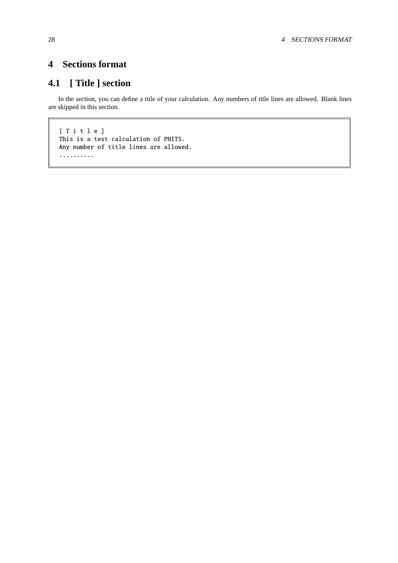
28 4 SECTIONS FORMAT
4 Sections format
4.1 [ Title ] section
In the section, you can define a title of your calculation. Any numbers of title lines are allowed. Blank linesare skipped in this section.
[ T i t l e ]
This is a test calculation of PHITS.
Any number of title lines are allowed.
..........

4.2 [ Parameters ] section 29
4.2 [ Parameters ] section
The various parameters of PHITS can be defined in[Parameters] using the following format:
[ P a r a m e t e r s ]
para1 = number | file.namepara2 = number | file.name..........
The order of parameters can be changed. As each parameter has a default value, undefined parameters use thedefault values.
Parameters and default values will be shown in the tables shown below.(D= ) indicates the default value.
4.2.1 Calculation mode
Table 4.1:Parameters (1)
Parameter Value Explanation
icntl (D=0) Basic control option.= 0 Normal PHITS calculation.= 1 Nuclear reaction calculation, (under development).= 3 Output only input echo for checking memory usage, and library, and file links.= 5 No reaction, no ionization. All regions are set to void for geometry check, and volume
and area calculations.= 6 Source check. Source positions can be tallied by[t-product].= 7 Execute[t-gshow] for graphical output.= 8 Geometry output ofxyzmesh tally with gshow option for graphical output.= 9 Execute[t-rshow] for graphical output.= 10 Geometry output ofregmesh tally with rshow option for graphical output.= 11 Execute[t-3dshow] for graphical output.= 12 Re-calculate usingdumpall file. Dumpall file is specified byfile(15).= 13 Use of function to sum up tally results (Sumtally function).= 14 Use of automatic calculation of region volume.= 15 Execute[t-wwbg] to obtain[ww bias] parameters.
The nuclear reaction calculation function specified asicntl=1 is still under development.By settingicntl=12, PHITS re-calculates the whole transport by reading the information from the dumpall
file, which is created by thedumpall=1 option. This re-calculation can be used to describe previously calculatedwhole transport events; to perform re-calculation, the input file from the previous calculation must be used;maxcas
andmaxbch cannot be changed, but are read from the file. This functionality is a very powerful tool for calculatingtallies that were not used in a previous calculation. However, it should be noted that calculation withdumpall=1
may create a hugedumpall file.By settingicntl=13, two (or more) tally results can be summed: see Sec.5.8for further detail.By settingicntl=14 with [t-volume], automatic calculations to obtain volumes of specified cells can be
performed. See Sec.7 in detail.By settingicntl=15 with [t-wwbg], automatic calculations to obtain parameters of[ww bias]. See Sec.
6.16in detail.

30 4 SECTIONS FORMAT
4.2.2 Number of history and Bank
Table 4.2:Parameters (2)
Parameter Value Explanation
irskip (D=0) Random number control.irskip>0 Begin calculation after skipping histories by number ofirskip (for debug).irskip<0 Begin calculation after skipping random numbers by number ofirskip (for man-
ual parallel computing).rseed (D=0.0) Initial random number option.
rseed<0 Get an initial random number from starting time.rseed=0 6647299061401 (default).rseed>0 Userseed as initial seed of random number.
maxcas (D=10) Number of history per 1 batch. The upper limit is 2147483647.maxbch (D=10) Number of batch. The upper limit is 2147483647.maxbnk (D=10000) Size of bank array.timeout (D=-1.0) CPU time to cut-off PHITS calculation [s].istdev (D=0) Control parameter for calculation of statistical uncertainties and restart mode.
=-2 Restart calculation mode is activated, but if there is no past tally result a new cal-culation is started withistdev=2.
=-1 Restart calculation mode is activated, but if there is no past tally result a new cal-culation is started withistdev=1.
=0 istdev is automatically set to 1 for shared-memory parallel computing, and 2 forthe other cases.
=1 A new calculation is begun. Statistical uncertainties are estimated from the vari-ances of each batch result.
=2 A new calculation is begun. Statistical uncertainties are estimated from the vari-ances of each history result. This option cannot be selected in shared-memoryparallel mode.
ireschk (D=0) Control parameter for tally consistency check.=0 Check consistency between new and old tally settings.=1 No check. This option is useful when setting a very complex tally whose settings
are not fully written in the tally output file.
In the distributed-memory parallel calculation, the number of batches should be an integer multiple ofNPE− 1,whereNPE is the total number of Processing Element (PE); otherwise, PHITS will automatically convertmaxbch
as it becomes to an integer multiple and adjustmaxcas as the total number of histories becomes almost same withgiven total histories. In this case, some comments will be output at the end of an input echo.
A time limit of a PHITS calculation can be set bytimeout. This function is available whentimeout ispositive. When a CPU time exceedstimeout at the last of one batch, PHITS finishes its calculation. In the casethat a CPU time exceedstimeout in the middle of one batch, PHITS continues the calculation until the end of thebatch. In the distributed-memory parallel computing, PHITS comparestimeout with the sum of all CPU time.Note that PHITS cannot get a correct CPU time depending on computers. In this case, you cannot use the functionof timeout.
The procedure for calculating statistical uncertainties was revised from version 2.50: a function to restartPHITS calculation based on the tally results obtained by past PHITS simulations has been implemented to increasethe total history number and then decrease the statistical uncertainties of the results. In this mode, the initial randomseed is also read from the past tally file.
To calculate statistical uncertainties, two modes can be selected - “batch variance mode” and “history variancemode” - which calculate standard deviation using the variances between tally results of each batch and history,

4.2 [ Parameters ] section 31
respectively. In both modes, standard deviationσ is calculated as
σ =
√√√√√√√√ N∑i=1
(xiwi/w)2 − NX2
N(N − 1)(1)
whereN is the total batch number (istdev=1) or the total history number (istdev=2), xi andwi are tally resultsand the source weight of each sample, respectively, andX and w are the mean values of the tally results andsource weights ofN samples, respectively. The ratio ofσ to X is written as relative error in the tally output file.In shared-memory parallel computing mode, only the batch variance mode can be selected as it is impossible tocalculate tallied quantities history-by-history using shared-memory parallel computing. The standard deviationscalculated by the batch variance mode vary by combination ofmaxcas andmaxbch, even for the same total historynumber. In principle, a largermaxbch provides more reliable statistical uncertainties in batch variance mode butmay require a longer computational time. We recommend settingmaxbch to more than 10 to obtain reliableresults. By contrast, in history variance mode, the standard deviation depends only on the total history number andis independent of the combination ofmaxcas andmaxbch. Thus, it is recommended that history variance mode(istdev=2) be selected when memory-shared parallel computing is not in use. Note, however, that computationaltime occasionally becomes extremely long in history variance mode, especially in cases in which there are talliesusing many memories, e.g.,xyz mesh tally with its very fine structure. In tallies for calculating the variance ofdeposition energies by individual history, such as[t-deposit] with output=deposit and[t-deposit2], thestandard errors instead of the standard deviations are output as relative errors. The relative standard errors can beestimated as 1/
√K whereK is the number of histories contributing to the tally result. This calculation procedure
is independent of theistdev parameter.Relative errors are generally output in the “r.err” column, which is the rightmost column of tally results.
In the case of 2D-plots, such as tallies withaxis=xy or rz, errors are output into another file, “*err”where“*” indicates the file name specified in the tally. For example, whenfile=tally.out, the name of the error fileis “tally err.out”. This error file has the same format of the conventional tally output file; hence, a graph for theerror in the 2D-plot can be obtained by ANGEL through a conversion process.
Note that the true value is not always within the error range because PHITS calculates the standard deviationor the standard error. The range means the 68% confidence interval. Furthermore, PHITS does not estimatesystematic uncertainties arising form the nuclear reaction model.
Whenistdev<0, the restart calculation mode is activated; however, if there is no past tally result, a newcalculation is started withistdev=|istdev|; in other words, the batch and history variance modes are selectedfor istdev=-1 and-2, respectively. When restarting a calculation, the variance mode is automatically determinedfrom the past PHITS calculation. Although the same tally parameters written in the past tally results must bewritten, new tallies can be added in the restart calculation. The procedure for restart calculation is as follows:
(1) Check whether or not the file specified byresfile in each tally section exists. The default file name of the“resfile” is that given byfile parameter.
(2) If there is no “resfile” for a tally, it is regarded to be new. If no “resfile” can be found for any tally, a newcalculation is begun withistdev=|istdev|.
(3) If “resfile” exists, PHITS reads information from the file on the variance modeistdev, total weightresc2,total history numberresc3, history number per batchmaxcas, the next random seedrijklst, and theresults and relative errors of the past calculation.
(4) The tally parameters given in the current and past PHITS input files are then checked for consistency. If theyare not consistent each, PHITS stops the calculation and outputs an error message. It should be noted thatnot all tally parameters are checked for consistency in this process.
(5) (In batch variance mode only) The consistency ofistdev andmaxcas among the “resfiles” is checked. Ifthey are consistent, the restart calculation is performed using these values. If an inconsistency is found, thecalculation is stopped.
(6) The initial random seed is changed to the value ofrijklst obtained from the first “resfiles”. Ifrijklstdiffers by “resfile”, a warning message is output.
(7) Upon finishing the restart calculation, the tally results are output to the file specified byfile=. If resfileis not specified, the past tally results are overwritten.

32 4 SECTIONS FORMAT
Important notice:
I. All past tally results should be calculated in the same variance mode: i.e.,istdev should be the same in all“resfile”.
II. Themaxcas written in the input file is not used in the restart calculation in batch variance mode.
III. Except for those given in the tally sections, the consistencies of input parameters are not checked. Hence,these must be set as identical by the operator in the restart calculation.
4.2.3 Cut-off energy and switching energy
Table 4.3:Parameters (3)
Parameter Value Explanation
emin(1) (D=1.0) Proton cut-off energy [MeV].emin(2) (D=1.0) Neutron cut-off energy [MeV].emin(i) (D=1.0) (i = 3 - 10) Cut-off energy for pions, muons, and kaons [MeV]. (i; particle
id, see Table3.4)emin(11) (D=2.0) Cut-off energy for others (MeV).emin(i) (D=1.e+9) (i= 12 - 14) Cut-off energy for electrons, positrons, and photons [MeV]. (i;
particle id, see Table3.4)emin(i) (D=1.0) (i= 15 - 19) Cut-off energy for deuterons, tritons,3He, 4He, and nuclei
[MeV/u]. emin for nuclei is defined in units of MeV per nucleon. (i; parti-cle id, see Table3.4)
esmin (D=0.001) Minimum energy for range calculation for the charged particles [MeV/u].esmax (D=300000) Maximum energy for range calculation for the charged particles [MeV/u].cmin(i) (D=emin(i)) Nuclear reaction cut-off energy fori-th particle [MeV]. Any nuclear reactions
undercmin(i) are not treated.i= 15 - 19 For these nuclei, energy unit is [MeV/u].
dmax(i) (D=emin(i)) Maximum energy of library use fori-th particle [MeV].etsmin (D=1e-6) Minimum energy of particles simulated by track structure mode [MeV].etsmax (D=1e-2) Maximum energy of particles simulated by track structure mode [MeV].
Values given by these parameters are included in lower limits but not in upper limits. For example, a protonright at theemin(1) energy is not cut-off.
PHITS uses libraries in the energy regionemin < energy< dmax. If emin>dmax is set, no libraries are used.The maximum energies for neutrons and photons are 20 MeV and 100 GeV, respectively. When EGS5 is not used,the maximum energies for electrons and positrons are 10 GeV.
The range table of charged particles is set withinesmin < energy< esmax. To use a significantly higherenergy, the user should setesmax.
The minimum cut-off energy for charged particles,emin, cannot be set lower thanesmin. In such cases,eminis automatically adjusted toesmin.etsmin>1e-9 (1meV) can be set. But the setting below 1e-6 (1eV) is not recommend because computational
time becomes extremely long.etsmax>1e-3 (1keV) must be set. The setting this parameter below 0.1 (100keV) is recommend, otherwise
the computational time becomes extremely long.For the track structure mode,emin(12) andemin(13) should be set to 1.0e-3, and EGS5 should be activated
(negs=1).

4.2 [ Parameters ] section 33
Table 4.4:Parameters (4)
Parameter Value Explanation
ejamnu (D=20.) Switching energy of nucleon-nucleus reaction calculation from Bertini (or QMD)to JAM model [MeV].
ejampi (D=20.) Switching energy of pion-nucleus reaction calculation from Bertini to JAM model[MeV].
eisobar (D=0.0) Maximum energy [MeV] of isobar calculation when isobar is defined(isobar=1).
eqmdnu (D=20.) Switching energy of nucleon-nucleus reaction calculation from Bertini to QMDmodel [MeV/u].
eqmdmin (D=10.0) Minimum energy of QMD calculation [MeV/u].ejamqmd (D=3000.0) Switching energy from JQMD to JAMQMD [MeV/u].inclg (D=1) Control parameter for use of INCL.
=0 INCL is not used.=1 Use of INCL in a proton, neutron, pion,d, t,3He, or4He induced reaction.=2 Use of INCL in a proton, neutron, or pion induced reaction.
einclmin (D=1.0) Minimum energy of INCL calculation [MeV/u].einclmax (D=3000.0) Maximum energy of INCL calculation [MeV/u].incelf (D=0) Control parameter for use of INC-ELF.
=0 INC-ELF is not used.=1 Use of INC-ELF in a proton or neutron induced reaction.
eielfmin (D=1.0) Minimum energy of INC-ELF calculation [MeV].eielfmax (D=3500.0) Maximum energy of INC-ELF calculation [MeV].irqmd (D=0) Control parameter for use of JQMD or JQMD-2.0.
=0 Use of JQMD in nuclear reactions.=1 Use of JQMD-2.0 in nuclear reactions.
Kerma (D=0) Option for Kerma mode.=0 This option is not used.=1 When neutron or proton nuclear data library of is used, PHITS produces no
charged particles except for protons.
Beloweqmdmin, the nuclear reactions ofd, t,3He,4He, and nuclei are not treated by QMD. As the applicabilityof QMD is restricted in the low energy region and the range of nuclei is very low in the normal material, it isnot necessary to consider the low energy reactions of nuclei for the usual case. As a default, high energy heavyion collisions are treated by JAMQMD above 3.0 GeV/u. This switching energy can be changed by changing ejamqmd. It is possible to calculate even nucleon-induced collisions in JAMQMD by changingeqmdnu, ejamnu,andejamqmd.
INCL (Intra-Nuclear Cascade of Liege) is a nuclear reaction model for nucleon (proton and neutron), pion, andlight-ion (d, t,3He, or 4He) induced reactions. From version 2.50, INCL is used by default for these reactions ifthe nuclear reaction model is not explicitly specified. Before using INCL results in a publication, please refer to adocument14 in the footnotes.
Intra-Nuclear Cascade with Emission of Light Fragment (INC-ELF) is a nuclear reaction model for nucleon-induced reactions. Before using results obtained by INC-ELF in a publication, please refer a document15 in thefootnotes.
JQMD and JQMD-2.0 are nuclear reaction models; in particular, they can be used to describe heavy-ion in-duced reactions. In PHITS Ver. 2.7 and later, JQMD-2.0 can be used as an alternative to the conventional JQMD.JQMD-2.016 describes reactions - particularly peripheral collisions - more reasonably than JQMD. Users shouldnote that JQMD-2.0 may take more than twice the CPU time required by JQMD.
14 A. Boudard, J. Cugnon, J.-C. David, S. Leray, and D. Mancusi, Phys. Rev C87, 014606 (2013).15 Y. Sawada, Y. Uozumi, S. Nogamine, T. Yamada, Y. Iwamoto, T. Sato, and K. Niita, Nucl. Instr. & Meth. B 291, 38-44 (2012).16 T. Ogawa, T. Sato, S. Hashimoto, D. Satoh, S. Tsuda, and K. Niita, Phys. Rev C92, 024614 (2015).

34 4 SECTIONS FORMAT
Nucleon Library INCL (inclg=1) JAM
(1MeV)emin(i)
(=emin)dmax(i)
(3.0GeV)einclmax
Pion INCL (inclg=1) JAM
(1MeV)emin(i)
Nucleus JQMD JAMQMD
(d, t, 3He, α) INCL (inclg=1)
(10MeV/u)eqmdmin
(3.0GeV/u)ejamqmd
Kaon, Hyperon JAM
(3.0GeV)einclmax
Figure 4.1:Map of Nuclear Reaction Models.
Table 4.5:Parameters (5)
Parameter Value Explanation
negs (D=-1) Option for electron, positron, and photon transport.=-1 Transport only photons based on the PHITS original algorithm. By selecting this op-
tion, emin(14) anddmax(14) are automatically set to 0.001 and 1000.0, respectively.If these parameters are directly specified in the input file, the specified parameters over-write the setting.
= 0 Ignore electron, positron, and photon transport.= 1 Transport electrons, positrons, and photons based on the EGS5 algorithm. By set-
ting this option,emin(12,13) andemin(14) are automatically set to 0.1 and 0.001,respectively, whiledmax(12-14) are set to 1000.0. If these parameters are directlyspecified in the input file, the specified parameters overwrite the setting.file(1) orfile(20) must be specified in this option.
nucdata (D=1) Option for automatic setting ofemin(2) anddmax(2) for the usage of nuclear datalibrary.
= 0 No adjustment (nuclear data are not used).= 1 Change the parameters suitable for JENDL-4.0, i.e.emin(2)=1.0e-10 and
dmax(2)=20.0. If these parameters are directly specified in the input file, the spec-ified parameters overwrite the setting.file(1) or file(7) must be specified in thisoption.

4.2 [ Parameters ] section 35
4.2.4 Cut-off time, cut-off weight, and weight window
Table 4.6:Parameters (6)
Parameter Value Explanation
tmax(i) (D=1.e+9) Cut-off time fori-th particle [nsec].i = 1-20 (i; particle id, see Table3.4).
wc1(i) (D=-0.5) Minimum weight fori-th particle.wc2(i) (D=wc1/2) Cut-off weight fori-th particle.swtm(i) (D=1.0) Minimum source weight fori-th particle.wupn (D=5) Maximum value of weight window is given by the product ofwupn × (minimum
value in[Weight Window] section). Here,wupn ≥ 2 should be set.wsurvn (0.6*wupn) Survival weight value. Here, 1< wsurvn < wupn should be set.mxspln (D=5) Maximum number of split and maximum multiple number of survival. Here,
mxspln > 1 should be set.mwhere (D=0) Where the weight window takes place.
-1: at nuclear reaction,0: both,1: at region crossing.iwwbias (D=0) Option for[ww bias].
= 0 Values defined in[ww bias] are not used.= 1 Values defined in[ww bias] are used. The[weight window] parameters mul-
tiplied by inverse of the defined biases in[ww bias] are used.
The cut-off time for each particle should be specified astmax(i) (in units of [nsec]). After arrival at the cut-offtime, the particle is killed; although this is not effective in the context of high energy particle transport, it is usefulfor low energy particle transport calculation.
A particle’s weight is affected by the importance, forced collisions, implicit captures, and weight windowfunctions. When the weight is lower than the user-defined weight cut off, a Russian roulette method is applied todetermine whether or not the particle is killed. This function is not available for particles defined in the weightwindow.
Under the Russian roulette method, when the weightwgt is lower than the product,wc2× R, of wc2 and theratioR of the importances at the source and current points (i.e., whenwgt < wc2 × R), the particle survives with aprobabilitywgt /(wc1×R), which is a function of the particle’s own weight,WGT. If the particle survives, its weightis changed towgt = wc1 × R. If wc1 andwc2 are negative, they are respectively set to|wc1| = swtm(i) and|wc2| = swtm(i).
Any particles or regions for which the user has not set importances are given default importances of 1.In this case ofiwwbias=1, the products of the multiplication are output in the input echo of[weight window],
and[ww bias] with off is output. If an input file without[ww bias] is used, all values of[ww bias] in theinput echo are set to 1.

36 4 SECTIONS FORMAT
4.2.5 Model option (1)
Table 4.7:Parameters (7)
Parameter Value Explanation
ielas (D=2) Elastic scattering option.= 0 Exclude elastic scatter.= 1 Include neutron elastic scatter.= 2 Include neutron and proton elastic scatter.
ielms (D=100) Number of angle group for elastic scattering.inmed (D=1) Nucleon-nucleon cross section options for Bertini model.
= 0 Free (nmtclb25.dat).= 1 Cugnon old (nmtclb95.dat).= 2 Cugnon new (nmtclb30.dat).
nevap (D=3) Options for evaporation model.= 0 Without evaporation model.= 1 Using DRES model.= 2 Using SDM model.= 3 Using GEM model.
ismm (D=0) Control parameter of Statistical Multi-fragmentation Model (SMM).= 0 SMM is not used.= 1 SMM is used. When a JQMD calculation is performed, switching time from JQMD
to GEM changes from 100fm/c, which is the default value, to 75fm/c.igamma17 (D=2) γ decay option for residual nuclei.
= 0 Withoutγ decay.= 1 With γ decay.= 2 With γ decay based on EBITEM model.= 3 With γ decay and isomer production based on EBITEM model.
isobar (D=0) Options for isobar model.= 0 Without isobar.= 1 With isobar.
ipreeq (D=0) Options for pre-equilibrium model whennevap=1.= 0 Without pre-equilibrium model.= 1 With pre-equilibrium model.
level (D=3) Level density option whennevap=1.= 1 8/A.= 2 With Baba’s parameters.= 3 With Ignatyuk’s parameters.
Note thatinmed=1 is the default value, which includes in-medium effect for nucleon-nucleon cross sections.Using the Statistical Multi-fragmentation Model (SMM), PHITS improves the accuracy of calculating the
production cross sections of light and medium-heavy fragments for collisions of heavy ions such as Pb or Hg orfor incident energies over 100 MeV/u. It should be noted that the computational time becomes high when usingthis model: see the references18 19 for details.
Settingigamma=3 enables obtaining of information on isomer production using[t-yield] with axis=chartor dchain: reference20 in the footnotes for details.
17 Prior to ver. 2.73,file(14)=trxcrd.dat is required forigamma=1-3.18 T. Ogawa, T. Sato, S. Hashimoto, and K. Niita, Nuclear Instruments and Methods in Physics Research A 723 (2013) 36-46.19 J.P. Bondorf, A.S. Botvina, A.S. Iljinov, I.N. Mishustin, and K. Sneppen, Physics Reports 257 (1995) 133-221.20 T. Ogawa, S. Hashimoto, T. Sato, and K. Niita, Nuclear Instruments and Methods in Physics Research B 325 (2014) 35-42.

4.2 [ Parameters ] section 37
4.2.6 Model option (2)Table 4.8:Parameters (8)
Parameter Value Explanation
ieleh (D=0) Options for electron and positron transport.= 0 No slowing down and no reaction in the energy region abovedmax(12).= 1 When the energy,e, is abovedmax(12), the weight value,wgt, is changed to
wgt= e/dmax(12), and then the transport calculation is performed with the en-ergy ofdmax(12).
ipnint (D=0) Options for photo-nuclear reaction. (Until ver. 2.30, this parameter wasipngdr.)= 0 This reaction mechanism is not taken into account.= 1 This reaction mechanism is taken into account, except for nuclear resonance fluo-
rescence.= 2 This reaction mechanism is taken into account, including nuclear resonance fluo-
rescence.(See notes below this table for polarization of incident photons.)
pnimul (D=1.0) Multiplying factor to increase sampling probability of photo-nuclear reaction.imucap (D=1) Options for capture reaction of negative-muons. Characteristic X-ray production
from muonic atoms and nuclear absorption is considered.= 0 This reaction mechanism is not taken into account.= 1 This reaction mechanism is taken into account.
imuint (D=1) Options for muon-induced nuclear reaction based on the virtual photon theory.= 0 This reaction mechanism is not taken into account.= 1 This reaction mechanism is taken into account.
imubrm (D=1) Options for muon-induced bremsstrahlung.= 0 This reaction mechanism is not taken into account.= 1 This reaction mechanism is taken into account.
imuppd (D=1) Options for muon-induced electron-positron pair production.= 0 This reaction mechanism is not taken into account.= 1 This reaction mechanism is taken into account.
emumin (D=200.0) Minimum energy of muon-induced nuclear reaction [MeV].emumax (D=1.0e+6) Maximum energy of muon-induced nuclear reaction [MeV].npidk (D=0) Treatment of negative-charged decay particles below cut-off energy.
= 0 Sets to absorbed by force.= 1 Sets to decayed.
imagnf (D=0) Options for magnetic field.= 0 Without Magnetic field.= 1 With Magnetic field. Note that, to correctly describe the trajectory as a curve by
tally, setitstep=1 and adjust the step length for the field bydeltm.ielctf (D=0) Options for electromagnetic field.
= 0 Without electromagnetic field.= 1 With electromagnetic field. Note that, to correctly describe the trajectory as a
curve by tally, setitstep=1 and adjust the step length for the field bydeltm.
For the nuclear resonance fluorescence included byipnint=2, polarization of incident photons can be specifiedusing sx,sy,sz in [source] when incident photons are polarized. The angular distribution of the scatteredphotons is determined with regard to the polarization.
Cross sections of the muon-induced nuclear reaction depend onemumin; if this is changed, the values of thecross sections also change in the whole energy range.
If a particle with a decay channel assumes a lower energy than cut-off, the particle decays completely. Negative-charged decay particles withnpidk=0, are forced to take reactions for the purposes of forced absorption. If it isnot absorbed, the particle is decayed.

38 4 SECTIONS FORMAT
4.2.7 Model option (3)
Table 4.9:Parameters (9)
Parameter Value Explanation
andit (D=0) ∆ angular distribution for Bertini.= 0 50% isotropic, 50% forward.= 1 All isotropic.= 2 All forward.
icxsni (D=0) Option for reaction, elastic, and total cross sections in nucleon-nucleus collisions.= 0 Pearlstein-Niita’s formula.= 1 KUROTAMA model.= 2 Sato’s formula.
icrhi (D=2) Option for total cross section for Nucleus-Nucleus collisions.= 0 Shen formula.= 1 NASA formula.= 2 KUROTAMA model.
icrdm (D=0) Option for total reaction cross section for deuteron-induced reactions.= 0 Same asicrhi.= 1 MWO formula.
icxspi (D=1) Option for total reaction cross section for pion-induced reaction.= 0 Geometrical formula.= 1 Hashimoto’s formula.
iidfs (D=0) Option for neutron-induced fission.= 1 Neutron multiplicityν and neutron energy spectrum are taken from a literature.
idwba (D=0) Option for DWBA spectra.= 0 Without discrete DWBA spectra.= 1 With discrete DWBA spectra.
The KUROTAMA model gives nucleon-nucleus and nucleus-nucleus reaction cross sections over a wide inci-dent energy region. See the paper shown in the footnote21 for details; in published results based the KUROTAMAmodel, please reference this document.
The MWO formula reproduces reaction cross sections of deuteron-induced reactions for incident energiesbelow 1GeV and target nuclei heavier than or equal to carbon. See the paper shown in the footnote22 for details;in published results based the MWO model, please reference this document.
From version 2.86, Hashimoto’s formula is used as the default model of pion-induced reaction cross sections.This is an empirical formula that reproduces cross section experimental data better than the old model specified byicxspi=0.
If iidfs=1 is specified, the multiplicityν and energy spectra of neutrons from neutron-induced fission takenfrom reference23 are used instead of the nuclear library data for the following 18 nuclei:U-238, Pu-238, Pu-240, Pu-242, Cm-242, Cm-244, Cf-252, Th-232, U-232, U-233, U-234, U-235, U-236, Np-237, Pu-239, Pu-241, Am-241, and Bk-249.
Settingidwba=1 adds the discrete spectra calculated by the Distorted Wave Born Approximation (DWBA) tothe neutron and proton spectra obtained using other nuclear reaction models for the following reactions:
7Li( p, n)7Be reactions at 30–400 MeV9Be(p,n)9B reactions at 10–50 MeV6,7Li(d,n)7,8Be and6,7Li(d, p)7,8Li reactions at 10–50 MeV9Be(d,n)10B and9Be(d, p)10Be reactions at 5–25 MeV12,13C(d,n)13,14 and12,13C(d, p)13,14C reactions at 10–50 MeV
21 K. Iida, A. Kohama, and K. Oyamatsu, J. Phys. Soc. Japan 76, 044201 (2007), and L. Sihveret al., Nucl. Instr. & Meth. B 334, 34-39(2014).
22 K. Minomo, K. Washiyama, and K. Ogata, J. Nucl. Sci. Technol. 54, 127-130 (2017).23 J. M. Verbeke, C. Hagmnn, and D. Wright, “Simulation of Neutron and Gamma Ray Emission from Fission and Photofission” UCRL-
AR-228518 (2014).

4.2 [ Parameters ] section 39
4.2.8 Model option (4)Table 4.10:Parameters (10)
Parameter Value Explanation
ndedx (D=3) Option fordE/dx of charged particle and nucleus.= 0 SPAR24 for nucleus, NMTC for the others.= 1 ATIMA 25 for nucleus and proton, NMTC for the others.= 2 SPAR for nucleus, proton, pion, and muon, NMTC for the others.= 3 ATIMA for all charged particles.
mdbatima (D=500) Maximum database size of ATIMA.dbcutoff (D=0.0) Energy cut-off of ATIMA database [MeV/u].ih2o (D=-1) Water (only for H2O) ionization potential option for ATIMA.
< 0 Default: 75 eV.> 0 Ionization potential for water [eV].
irlet (D=1) Option fordE/dx of charged particle and nuclei with the function ofδ-ray gener-ation.
= 0 Conventional method (subtract the energy of sampledδ-ray from the unrestrictedstopping power).
= 1 Restricted LET.nspred (D=0) Option for Coulomb diffusion (angle straggling)26.
= 0 Without Coulomb diffusion.= 1 With Coulomb diffusion following the original NMTC model.= 2 With Coulomb diffusion following Lynch’s formula based on the Moliere the-
ory27(recommended).= 10 With Coulomb diffusion by ATIMA.
ascat1 (D=13.6) S2 parameter in Lynch’s formula fornspred=2.ascat2 (D=0.038) ϵ parameter in Lynch’s formula fornspred=2.nedisp (D=0) Energy straggling option for charged particle and nuclei.
= 0 Without energy straggling.= 1 With Landau Vavilov energy straggling28(recommended).= 10 With energy straggling for ATIMA.
Note that the default option forndedx wasndedx=0 until PHITS ver. 2.00 andndedx=2 between ver. 2.01and 2.85.
From version 2.85, the algorithm for calculating stopping power of ATIMA in PHITS was improved. In theolder algorithm, calculation of range and stopping power was always performed each time a new charged particlewas produced or a transporting particle entered a new material. The new algorithm creates a database for eachcombination of transporting particle and material when a new particle appears and refers to it the next time. Thus,the number of calls of the high cost routine ATIMA is reduced. Based on this improvement, PHITS simulationusing a high-precision ATIMA is now possible in the almost the same calculation time as is needed by SPAR.
After ver. 2.97, the settingndedx=3 can be used for nuclei with the mass number of 93≤ Z ≤ 97 (from Np toBk), 29. In the extention, ionization potential and density correction parameter shown in the reference30 are usedfor the nuclei in calculation of the nuclear stopping power, and SPAR is used in the calculation of the electronicstopping power.
24 T.M. Armstrong and K.C. Chandler, ORNL Report, ORNL-4869 (1973).25 About ATIMA, see the web site: https://web-docs.gsi.de/ weick/atima/26 When describing a scattering process on thin films less than 1cm,delt0 should be set to 1/10 of its thickness.27 σ = S2
√X/X0pβ [1 + ϵ log10(e) loge(X/X0)]: Eq.(4) in G.R. Lynch and O.I. Dahl, Nucl. Instrum. Methods Phys. Res, B 58, 6-10 (1991).
28 About these models, see the web site: http://www.dnp.fmph.uniba.sk/cernlib/asdoc/geantold/H2GEANTPHYS332.html29 Before ver. 2.96, for nuclei with larger mass number thanZ = 92 (U), ATIMA cannot be used. In this case, use SPAR by settingndedx=2.30 Table I of R.M.Sternheimer, Atomic data and nuclear data tables, 30, 261-271 (1984).
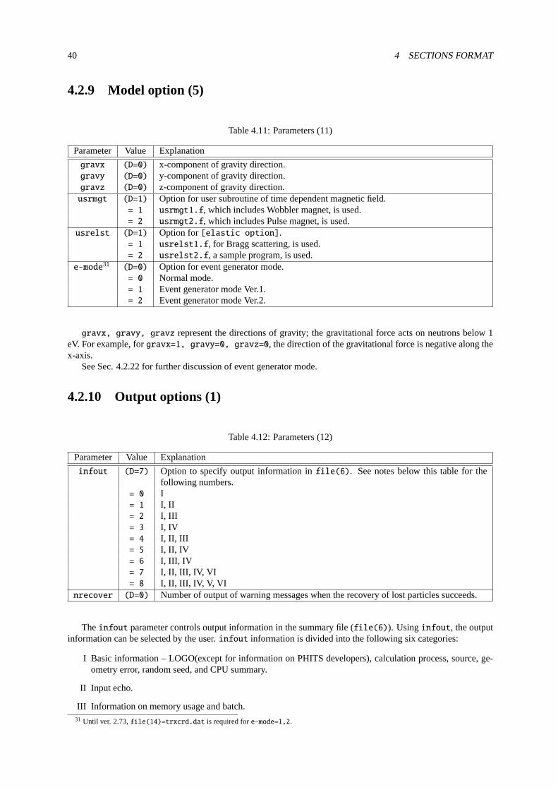
40 4 SECTIONS FORMAT
4.2.9 Model option (5)
Table 4.11:Parameters (11)
Parameter Value Explanation
gravx (D=0) x-component of gravity direction.gravy (D=0) y-component of gravity direction.gravz (D=0) z-component of gravity direction.usrmgt (D=1) Option for user subroutine of time dependent magnetic field.
= 1 usrmgt1.f, which includes Wobbler magnet, is used.= 2 usrmgt2.f, which includes Pulse magnet, is used.
usrelst (D=1) Option for[elastic option].= 1 usrelst1.f, for Bragg scattering, is used.= 2 usrelst2.f, a sample program, is used.
e-mode31 (D=0) Option for event generator mode.= 0 Normal mode.= 1 Event generator mode Ver.1.= 2 Event generator mode Ver.2.
gravx, gravy, gravz represent the directions of gravity; the gravitational force acts on neutrons below 1eV. For example, forgravx=1, gravy=0, gravz=0, the direction of the gravitational force is negative along thex-axis.
See Sec.4.2.22for further discussion of event generator mode.
4.2.10 Output options (1)
Table 4.12:Parameters (12)
Parameter Value Explanation
infout (D=7) Option to specify output information infile(6). See notes below this table for thefollowing numbers.
= 0 I= 1 I, II= 2 I, III= 3 I, IV= 4 I, II, III= 5 I, II, IV= 6 I, III, IV= 7 I, II, III, IV, VI= 8 I, II, III, IV, V, VI
nrecover (D=0) Number of output of warning messages when the recovery of lost particles succeeds.
Theinfout parameter controls output information in the summary file (file(6)). Usinginfout, the outputinformation can be selected by the user.infout information is divided into the following six categories:
I Basic information – LOGO(except for information on PHITS developers), calculation process, source, ge-ometry error, random seed, and CPU summary.
II Input echo.
III Information on memory usage and batch.31 Until ver. 2.73,file(14)=trxcrd.dat is required fore-mode=1,2.

4.2 [ Parameters ] section 41
IV Information on transport particles.
V Detailed information – variance reduction, number of scattered particles for each region, information foreach material.
VI Information on PHITS developers.
The information is output in the following order:
(1) LOGO (Category I – note that the only developer information is in category VI). Version of PHITS, devel-opers, job title, and starting time.
(2) Input echo (Category II). Echo of input file.
(3) Information on used memory (Category III).Amount of memory used for geometry, material, tally, bank, etc.
(4) Information on batch (Category III)Number of histories by batch and CPU time.
(5) Information on calculation process (ncol) (Category I).Number of geometry boundary crossings, reactions, termination by energy cut-off, etc.
(6) Information on variance reduction (Category V).Particle weights changed by importance, weight window, and forced collision options.
(7) Number of scattered particles for each region (Category V).
(8) Number of scattered particles for each material (Category V).
(9) Number of transport, produced, stop, and leakage particles (Category IV).
(10) Number of source particles and their weights (Category I).
(11) Geometry error (Category I).Number of lost particles and their types.
(12) Random seed (Category I).Initial random seed and next initial random seed.
(13) CPU summary (Category I).Total computation time and number of calls for each calculation process. The meanings of the items are asfollows (whenicput=0, information on the computation time, except for “total cpu time”, is not output;neither are “transport” or “set data” items):
• total cpu time: total computation time.
• transport: time for particle transport.
• set data: time for setting input parameters.
• analysis: number of data processing events.
• nevap: number of evaporations.
• dexgam: number of de-excitations.
• nreac: number of atomic and nuclear reactions.
• dklos: number of particle decays.
• hydro: number of nucleon-nucleon scatterings.
• n-data: number of runs using neutron data library.
• h-data: number of runs using proton data library.
• p-data: number of runs using photon data library.
• e-data: number of runs using electron data library.
• p-egs5: number of photon interactions with EGS5.

42 4 SECTIONS FORMAT
• e-egs5: number of electron interactions with EGS5.
• photonucl: number of photo-nuclear reactions.
• muon: number of muon-induced nuclear reactions.
• elast: number of elastic scatterings.
• ncasc: number of runs using nuclear reaction model.
• bertini: number of runs using Bertini model.
• isobar: number of runs using isobar model.
• JAM: number of runs using JAM model.
• QMD: number of runs using JQMD or JQMD-2.0 models.
• JAMQMD: number of runs using JAMQMD model.
• INCL: number of runs using INCL model.
• INCELF: number of runs using INC-ELF model.
Wheninfout=8, information on the calculations by each nuclear reaction model is output in detail.
• count: number of runs using the model with each incident particle.
• real: number of successes for model calculation.
• %: probability of model calculation.

4.2 [ Parameters ] section 43
4.2.11 Output options (2)
Table 4.13:Parameters (13)
Parameter Value Explanation
incut (D=0) Neutron output options below cut-off.= 0 No output.= 1 Output in the ncut file specified asfile(12).= 2 Output infile(12) with time information.
igcut (D=0) γ-ray and electron output options below cut-off.= 0 No output.= 1 Outputγ-ray data in thegcut file specified asfile(13).= 2 Outputγ-ray infile(13) with time information.= 3 Outputγ-ray, electron, and positron data infile(13).
ipcut (D=0) Proton output options below cut-off.= 0 No output.= 1 Output in the pcut file specified asfile(10).= 2 Output infile(10) with time information.
inpara (D=0) ncut file name options in the parallel calculation.= 0 /wk/uname/file-name offile(12).= 1 /wk/uname/file-name offile(12)+(PE number).= 3 File-name offile(12)+(PE number).
igpara (D=0) gcut file name options in the parallel calculation.= 0 /wk/uname/file-name offile(13).= 1 /wk/uname/file-name offile(13)+(PE number).= 3 File-name offile(13)+(PE number).
ippara (D=0) pcut file name options.= 0 /wk/uname/file-name offile(10).= 1 /wk/uname/file-name offile(10)+(PE number).= 3 File-name offile(10)+(PE number).
/wk/uname/ /wk/ is the default directory name.uname is a user-name read in from the environment variableLOGNAME.
iMeVperu (D=0) Option for unit of energy in output of tally.=0 Output as unit of MeV.=1 Output as MeV/u (MeV per nucleons). Note that the unit means MeV for particles
other than nuclei.
Note that the defaults ofincut andigcut have been changed 0.In parallel computing, files corresponding to each PE (Processor Element) are created for writing the output. If
inpara, igpara, or ippara are set= 0 or 1, a file is made in the directory named by/wk/uname/ on each of thenodes. Ifinpara, igpara, or ippara are set= 1 or 3, each PE number is put at the end of the filename. EachPE writes down its result on only the corresponding file.
WheniMeVperu=1, the unit of nucleus energy is changed from [MeV] to [MeV/u] in outputs of[t-track],[t-cross], [t-point], [t-product], [t-time], [t-star]. For example, in the case of[t-track]withunit=2, quantities in units of [1/cm2/MeV/source] are converted to those in [1/cm2/(MeV/u)/source].

44 4 SECTIONS FORMAT
4.2.12 Output option (3)
Table 4.14:Parameters (14)
Parameter Value Explanation
itall (D=0) Options for tally output after every batch.= -1 No output.= 0 Output only numerical data files.= 1 Output both numerical data and image (*.eps) files32.
itstep (D=0) Option for timing of tally for changing momentum, such as magnetic field.= 0 Tally at reaction or surface cross (normal).= 1 Tally at each step of the transport.
imout (D=0) Option for specifying the output format of[material] section.= 0 e.g.,mat[12], 208Pb.33c.= 1 e.g.,mat[12], Pb-208.33c.= 2 e.g.,m12, 82208.33c (MCNP type).
jmout (D=0) Option for specifying the output format of material density in[material].= 0 No conversion.= 1 Conversion into particle density.= 2 Conversion into mass ratio (%).
kmout (D=0) Option of nuclear data information.= 0 No display.= 1 Writing in input echo.33
matadd (D=1) Treatment of varying densities in a given material.= 0 Use of same material number.= 1 Use of new material number.
natural (D=1) Option for distribution according to natural isotope ratio, when elements without massnumber are defined in[material].
= 0 Not distributed.= 1 Distributed. Distributed isotopes are not output infile(6).= 2 Distributed. Distributed isotopes are output infile(6).
Normally, the tallies are called at the reaction point or the surface crossing; thus, the particle track in, forexample, the magnetic field is shown as a straight line between collisions or between one collision and a surfacecrossing. To describe the trajectory correctly as a curve, setitstep=1 and adjust the step length for the field bydeltm.
When defining two (or more) cells of differing densities with the same material number, all cells except for thefirst are given other material numbers bymatadd=1 (the default setting). Ifmatadd=0 is set, the cells have thesame material number. Note that this setting is invalid in the[mat name Color], in which other given materialnumbers, which are output as a warning message in the first part offile(6) (D=phits.out), are output.
32 Note that vtk files are output with bothitall=0,1.33 From Ver. 2.86, thedmax of each nucleus is also output.

4.2 [ Parameters ] section 45
4.2.13 Output option (4)
Table 4.15:Parameters (15)
Parameter Value Explanation
iggcm (D=0) Option of GG warnings.= 0 No echo.= 1 In input echo.
ivout (D=0) Volume display options in the input echo.= 0 In [volume].
ipout (D=1) Importance display options in the input echo.(D=0 for GG)
= 0 In [importance]. (this function is only available when all particles are set tothe same importance value.)
icput (D=0) CPU time count options.= 0 Without count.= 1 With count.
ipara (D=0) Parameter display options.= 0 Only described parameters.= 1 All parameters.
nwsors (D=0) Write down the information onnwsors source particles infile(6).dumpall (D=0) dumpall option.
= 0 No dump.= 1 Write down all information onfile(15) as binary data.= -1 Write down all information onfile(15) as ASCII data.
idpara (D=3) dumpall file name option in the parallel calculation.= 0 /wk/uname/file-name offile(15).= 1 /wk/uname/file-name offile(15)+(PE number).= 3 File-name offile(15)+(PE number).
/wk/uname/ /wk/ is the default directory name.uname is a user-name read in from the environment variableLOGNAME.
To save calculation time, CPU time counting is not available by default; to obtain the CPU time for eachprocess, seticput=1.
Settingipara=1 enables confirmation of all parameters in the PHITS code.Settingicntl=12 causes PHITS to recalculate the whole transport by reading the information from thedumpall
file, which is created if thedumpall option is used. The recalculation can describe whole transport events thatwere previously calculated. The same input file as was used in the previous calculation is required;maxcas andmaxbch cannot be changed, but are read from the file. This functionality is very powerful for calculating tallies thatwere not used in a previous calculation; however, calculation with thedumpall option may create a hugedumpallfile. This option is only available for GG geometry.
In parallel computing, files corresponding to each PE (Processor Element) are created for writing and readingdumped data. Ifidpara is set= 0 or 1, a file named by/wk/uname/ is made in the directory on each of the nodes.If idpara is set= 1 or 3, each IP number is placed at the end of the filename. Each PE writes down its result onlyon the corresponding file and reads it from the same file during recalculation.

46 4 SECTIONS FORMAT
4.2.14 Output option (5)
Table 4.16:Parameters (16)
Parameter Value Explanation
ivoxel (D=0) Read and write voxel data in binary.=0 Not usingfile(18).=1 Read from voxel data in binaryfile(18).=2 Write down voxel data in binary onfile(18).
itetvol (D=0) Option to compute volume of tetrahedron geometry forLAT=3.=0 The volume will not be computed.=1 The volume will be automatically computed and used in tallies, etc.
itetra (D=0) Read and write tetrahedron geometry data in binary.=0 Not using the data file.=1 Read from tetrahedron geometry data in binaryTetra.bin (fixed name).=2 Write down tetrahedron geometry data in binaryTetra.bin (fixed name).
ntetsurf (D=100) Number of outer surfaces of tetrahedron geometry allowed for each sub-space of thecontainer box.
ntetelem (D=200) Number of elements of tetrahedron geometry allowed for each sub-space of the con-tainer box.
The ivoxel parameter can be used to enable time shortening. When performing PHITS calculation withivoxel=2, voxel data are output infile(18) in binary and the calculation is stopped (until ver. 2.30, calculationwas continued). From the next calculation withivoxel=1, a data output process is omitted and the calculationtime is shortened.
When the tetrahedron geometry is treated withLAT=3, the volume of the universes appearing in tetrahedrongeometry can be automatically computed using the optionitetvol=1. However, the volume is computed bysimply summing up the volumes of individual tetrahedrons, which might produce incorrect values in cases inwhich tetrahedron geometry is clipped out through the use of the universe and fill nest structure. The computedvalue is given priority over values specified in the volume section, etc., by setting the optionitetvol=1.
When tetrahedron geometry (LAT=3) is used in PHITS calculation, necessary information for transport calcula-tion is generated by reading the tetrahedron geometry file prior to the actual transport calculation. This process willbecome computationally heavy as the number of elements in the tetrahedron geometry increases. In this case, theitetra parameter can be used to reduce the computational time. Performing PHITS calculation withitetra=2
causes the processed tetrahedron geometry data to be recorded in a binary file (Tetra.bin) and then stops thecalculation. From the next calculation withitetra=1, the necessary information is read from theTetra.bin fileand the data generation process is omitted to reduce the calculation time.
For PHITS calculation with tetrahedron geometry (LAT=3), two algorithms sub-dividing the box containingthe tetrahedron geometry are introduced to reduce the computational time of transport calculation by limiting thenumber of elements belonging to each sub-space. One algorithm finds a surface of the tetrahedron geometry whena particle enters the geometry. The container box is sub-divided so that the number of outer surfaces at eachsub-space is less thanntetsurf. The other algorithm finds an element of tetrahedron geometry when a particleis initiated inside the geometry. The box containing all tetrahedron elements is subdivided so that the number ofelements belonging to each sub-space is less thanntetelem.

4.2 [ Parameters ] section 47
4.2.15 About geometrical errors
Table 4.17:Parameters (17)
Parameter Value Explanation
nlost (D=10) Acceptable value against lost particle (per 1 PE).igerr (D=0) Number of recoveries for region error.igchk (D=0) =0: no region check.
=1: check region setting flight mesh todeltb after region-crossing.deltb (D=1.e-9) Flight mesh [cm] after region-crossing withigchk=1. (this is also the dis-
tance from the region boundary where the particle is created by importance andforced collision.)
deltm (D=20.12345) Maximum flight mesh [cm]. Linked withidelt.deltc (D=2.012345) Maximum flight mesh [cm] for charged particles withnedisp=1,10. Linked
with idelt.delt0 (D=0.1) Minimum flight mesh [cm] withnspred=1,2,10. Note that, when describing
a scattering process on thin films less than 1 cm,delt0 should be set to 1/10of its thickness.
deltg (D=1.012345) Maximum flight mesh [cm] on magnetic field.deltt (D=1.0) Maximum flight time [msec] on time-dependent magnetic field.idelt (D=1) Option for minimum flight mesh:
=0: Use values ofdeltm anddeltc as flight mesh maxima.=1: Maximum flight mesh isdeltm anddeltc divided by the density in theregion.
From ver. 2.80,idelt=1 is the default setting of PHITS. In this case, the quotients ofdeltm anddeltcdivided by the region’s density are used as the flight mesh maxima. This setting is useful in the time shortening ofparticle transport calculation in air over several hundred meters.
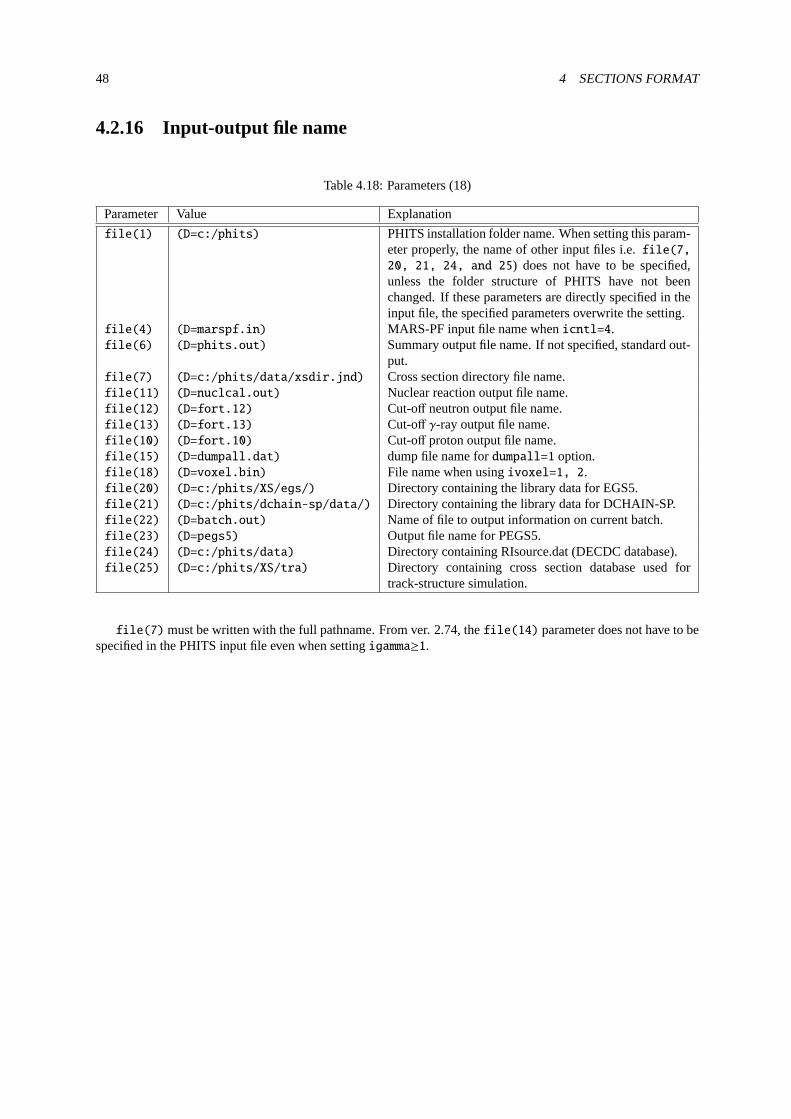
48 4 SECTIONS FORMAT
4.2.16 Input-output file name
Table 4.18:Parameters (18)
Parameter Value Explanation
file(1) (D=c:/phits) PHITS installation folder name. When setting this param-eter properly, the name of other input files i.e.file(7,20, 21, 24, and 25) does not have to be specified,unless the folder structure of PHITS have not beenchanged. If these parameters are directly specified in theinput file, the specified parameters overwrite the setting.
file(4) (D=marspf.in) MARS-PF input file name whenicntl=4.file(6) (D=phits.out) Summary output file name. If not specified, standard out-
put.file(7) (D=c:/phits/data/xsdir.jnd) Cross section directory file name.file(11) (D=nuclcal.out) Nuclear reaction output file name.file(12) (D=fort.12) Cut-off neutron output file name.file(13) (D=fort.13) Cut-off γ-ray output file name.file(10) (D=fort.10) Cut-off proton output file name.file(15) (D=dumpall.dat) dump file name fordumpall=1 option.file(18) (D=voxel.bin) File name when usingivoxel=1, 2.file(20) (D=c:/phits/XS/egs/) Directory containing the library data for EGS5.file(21) (D=c:/phits/dchain-sp/data/) Directory containing the library data for DCHAIN-SP.file(22) (D=batch.out) Name of file to output information on current batch.file(23) (D=pegs5) Output file name for PEGS5.file(24) (D=c:/phits/data) Directory containing RIsource.dat (DECDC database).file(25) (D=c:/phits/XS/tra) Directory containing cross section database used for
track-structure simulation.
file(7)must be written with the full pathname. From ver. 2.74, thefile(14) parameter does not have to bespecified in the PHITS input file even when settingigamma≥1.
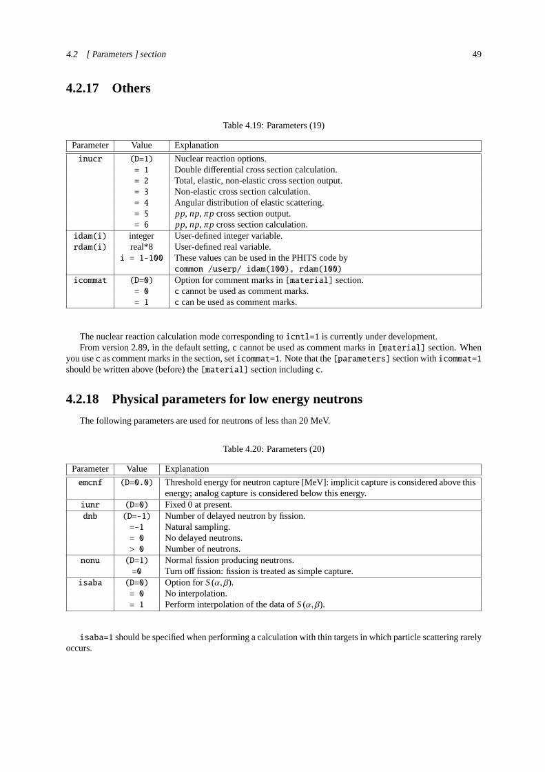
4.2 [ Parameters ] section 49
4.2.17 Others
Table 4.19:Parameters (19)
Parameter Value Explanation
inucr (D=1) Nuclear reaction options.= 1 Double differential cross section calculation.= 2 Total, elastic, non-elastic cross section output.= 3 Non-elastic cross section calculation.= 4 Angular distribution of elastic scattering.= 5 pp, np, πp cross section output.= 6 pp, np, πp cross section calculation.
idam(i) integer User-defined integer variable.rdam(i) real*8 User-defined real variable.
i = 1-100 These values can be used in the PHITS code bycommon /userp/ idam(100), rdam(100)
icommat (D=0) Option for comment marks in[material] section.= 0 c cannot be used as comment marks.= 1 c can be used as comment marks.
The nuclear reaction calculation mode corresponding toicntl=1 is currently under development.From version 2.89, in the default setting,c cannot be used as comment marks in[material] section. When
you usec as comment marks in the section, seticommat=1. Note that the[parameters] section withicommat=1should be written above (before) the[material] section includingc.
4.2.18 Physical parameters for low energy neutrons
The following parameters are used for neutrons of less than 20 MeV.
Table 4.20:Parameters (20)
Parameter Value Explanation
emcnf (D=0.0) Threshold energy for neutron capture [MeV]: implicit capture is considered above thisenergy; analog capture is considered below this energy.
iunr (D=0) Fixed 0 at present.dnb (D=-1) Number of delayed neutron by fission.
=-1 Natural sampling.= 0 No delayed neutrons.> 0 Number of neutrons.
nonu (D=1) Normal fission producing neutrons.=0 Turn off fission: fission is treated as simple capture.
isaba (D=0) Option forS(α, β).= 0 No interpolation.= 1 Perform interpolation of the data ofS(α, β).
isaba=1 should be specified when performing a calculation with thin targets in which particle scattering rarelyoccurs.

50 4 SECTIONS FORMAT
4.2.19 Physical parameters for photon and electron transport based onthe original model
Table 4.21:Parameters (21)
Parameter Value Explanation
emcpf (D=100) Maximum energy in the detailed photon model [MeV].ides (D=1) Electron creation options by photon.
= 0 Create electron or brems.photon.= 1 Do not create electron.
Note thatides automatically becomes 0 whenemin(12) or emin(13) is defined inthe input file (after ver. 2.96).
nocoh (D=0) Photon coherent scattering options.= 0 With coherent scattering.= 1 Without coherent scattering.
iphot (D=0) Photon creation options by electron.= 0 Create photon.= 1 Do not create photon.
ibad (D=0) Angular distribution option for brems.= 0 Full brems. tabular angular distribution.= 1 Simple brems. angular distribution approximation.
istrg (D=0) Straggling.= 0 Sampled straggling for electron energy loss.= 1 Expected value straggling for electron energy loss.
bnum (D=1) Brems. photon.= 0 Do not create brems. photon.> 0 Number of analog brems. photons.
xnum (D=1) X-ray photon.= 0 Not create X-ray photon.> 0 Number of analog X-ray photons.
enum (D=1) Secondary electron.= 0 Do not create secondary electron.> 0 Number of analog secondary electrons.
numb (D=0) Brems. process.= 0 Nominal brems. production.> 0 Produce brems. on each substep.
rnok (D=1) Knock-on electron.= 0 Do not create knock-on electron.> 0 Number of knock-on electrons.

4.2 [ Parameters ] section 51
4.2.20 Parameters for EGS5
Table 4.22:Parameters (22)
Parameter Value Explanation
ipegs (D=0) Option for controlling PEGS5. Too change the input file of PEGS5 (pegs5.inp),the operator must change this parameter. The parameter is not valid whennegs, 1.Note that, to retain PEGS5-related files after executing PHITS,iegsout automaticallybecomes 1 (or greater) whenipegs is set≤ 1.
= -1 Output PEGS5.inp: Yes, Execute PEGS5: Yes, Execute PHITS: No.= 0 Output PEGS5.inp: Yes, Execute PEGS5: Yes, Execute PHITS: Yes.= 1 Output PEGS5.inp: No, Execute PEGS5: Yes, Execute PHITS: Yes.= 2 Output PEGS5.inp: No, Execute PEGS5: No, Execute PHITS: Yes.
imsegs (D=1) Option for treating multiple scatterings in EGS5.= 0 Original EGS5 method. Under this option, the starting scattering strength is used only
when the electron is generated as a source particle. After several steps, the maximumscattering strength is used.
= 1 Original PHITS-EGS5 method. Use starting scattering strength whenever an electronenters a new material. This option enables simulation of the motion of an electronin thin foil without changing thechard parameter; the computational time becomesslightly longer.
iegsout (D=0) Option for controlling EGS5 output files.= 0 Delete all EGS5 output files when PHITS calculation is finished. Some files remain
when the user self-terminates the PHITS calculation.= 1 Keepegs5.inp, pegs5.dat andpegs5.msfit and delete the others.= 2 Keep all EGS5 output files. See EGS5 manual34for details on each file.
iegsrand (D=-1) Option for random number used in EGS5. Setting parameter to 0 or to a positive valuehides the MPI parallelization and the restart-calculation function.
< 0 Use random number generated by PHITS.= 0 Use random number generated by EGS5 with the default initial random seed
(314159265).> 0 Use random number generated by EGS5 with the initial random seed= iegsrand.
When using EGS5, the default values of the minimum and maximum energies for electron, positron, andphoton transports are changed toemin(12,13) = 0.1, emin(14) = 0.001, and dmax(12-14)=1,000.0,respectively. These values can also be changed by explicitly setting the related parameters. Note that the defaultvalues of several EGS5 parameters differ from those employed in the original EGS5 code.
From ver. 2.76, photo-nuclear reactions can be considered in using EGS5. Thus, input files withnegs=1 andipnint=1 produce results that differ from those calculated by the previous version of PHITS.
34 H. Hirayamaet al., SLAC-R-730 (2005) and KEK Report 2005-8 (2005).

52 4 SECTIONS FORMAT
Table 4.23:Parameters (23)
Parameter Value Explanation
iedgfl (D=1) Option for K and L-edge fluorescent photons.= 0 Do not explicitly treat K and L-edge fluorescent photons.= 1 Explicitly treat K and L-edge fluorescent photons.
iauger (D=1) Option for K and L-edge Auger electrons.= 0 Do not explicitly treat K and L-edge Auger electrons.= 1 Explicitly treat K and L-edge Auger electrons.
iraylr (D=1) Option for coherent (Rayleigh) scattering.= 0 Do not consider coherent scattering.= 1 Consider coherent scattering.
lpolar (D=0) Option for linearly polarized photon scattering (NOT valid at this moment).= 0 Do not consider linearly polarized photon scattering.= 1 Consider linearly polarized photon scattering.
iunrst (D=0) Option for output-stopping powers by PEGS5. When this parameter is changed,ipegs must be set to= −1; otherwise incorrect results will be obtained from thePHITS simulation.
= 1 Unrestricted collision only.= 2 Unrestricted collision and radiative.= 3 Unrestricted collision, restricted radiative.= 4 Restricted collision, unrestricted radiative.= 5 Unrestricted radiative only.= 6 Restricted radiative only.= 7 Restricted collision only.
chard (D=0.1) Array of “characteristic dimensions”, or representative size (in cm) of each material.This parameter controls the electron step-size in each material. The value must bedecreased when simulating electron scattering in thin foil by settingimsegs=0. Whena negative value is set for this parameter, the actualchard values used in EGS5 areadjusted to their absolute values divided by the material density in g/cm3. This optionis useful for simulating electrons in huge objects (of km order).
epstfl (D=0) Option for using density correction factors contained in EPSTAR.= 0 Do not use EPSTAR for density correction.= 1 Use EPSTAR for density correction. If this option is selected, a text file named
epstar.datmust be created in the same folder containing the PHITS input file. Thedata contained inXS/density correctionsmust be copied and paste pasted in theorder of materials specified in the[material] section. This can be directly changedfor each material by editingpegs5.inp.

4.2 [ Parameters ] section 53
Table 4.24:Parameters (24)
Parameter Value Explanation
incohr (D=1) Option for incoherent scattering function.= 0 Do not use incoherent scattering function for Compton scattering.= 1 Use incoherent scattering function for Compton scattering (ibound automatically be-
comes 1).iprofr (D=1) Option for Doppler broadening of Compton scattering energies.
= 0 Do not consider Doppler broadening.= 1 Consider Doppler broadening (incohr andibound automatically become 1).
impacr (D=1) Option for electron-impact ionization (EII).= 0 Do not consider EII.= 1 Consider EII.
ieispl (D=0) Option for splitting of X-rays generated by electron-impact ionization.= 0 No splitting.= 1 Splitting.
neispl (D=0) Number of electron-impact ionization X-rays for splitting whenieispl=1.ibrdst (D=1) Option for determining of bremsstrahlung polar angle.
= 0 Angle given bym/E.= 1 Sampling.
iprdst (D=1) Option for determining of polar angles of pair electrons.= 0 Angle given bym/k.= 1 Sampling.
iphter (D=1) Option for determining angular distributions of photoelectrons.= 0 Emission in direction of incident photon.= 1 Sampling.
ibound (D=1) Option for Compton cross section.= 0 Use free Compton cross section.= 1 Use bound total Compton cross section.
iaprim (D=1) Option for correcting bremsstrahlung cross section.= 0 Use Motzet al. empirical.= 1 Normalize integrated cross section to ICRU-37 radiative stopping power.= 2 No correction.

54 4 SECTIONS FORMAT
4.2.21 Dumpall option
By icntl=12, PHITS re-calculates whole transport by reading the information from dumpall file, which is cre-ated if you use thedumpall option. The re-calculation can describe whole transport events which were calculatedbefore. One needs the same input file as used in the previous calculation.maxcas andmaxbch cannot be changed,but are read from the file. It is very powerful when you want to calculate different tallies which are not used inthe previous calculation. However, please be careful that the calculation with thedumpall option may create hugedumpall file. This option is only available for GG geometry.
The dumped data written in binary can be not used on the other computer. The data sequence and meaning aregiven in the following.
(1) NCOLNCOL is an intrinsic variable in the program and denotes identification of process.
NCOL1 : start of calculation2 : end of calculation3 : end of a batch4 : source5 : detection of geometry error6 : recovery of geometry error7 : termination by geometry error8 : termination by weight cut-off9 : termination by time cut-off
10 : geometry boundary crossing11 : termination by energy cut-off12 : termination by escape or leakage13 : (n,x) reaction14 : (n,n’x) reaction15 : sequential transport only for tally
When NCOL=1, 2, 3, the output is finished. The followings are for NCOL≥4.
(2) NOCAS, NOBCH, RCASC, RSOUINThese four data are written only for NCOL=4 and their meaning are,
NOCAS : current history number in this batchNOBCH : current batch numberRCASC : real number of NOCAS+maxcas*(NOBCH-1)RSOUIN : sum of the weight of source particle
(3) NO, MAT, ITYP, KTYP, JTYP, MTYP, RTYP, OLDWTThese mean
NO : cascade id in this historyMAT : material idITYP : particle typeKTYP : particle kf-codeJTYP : charge number of the particleMTYP : baryon number of the particleRTYP : rest mass of the particle (MeV)OLDWT : weight of the particle at (x,y,z)
(a) QSThis data is written only for ITYP=12, 13, namely electron and positron. QS is dE/dx for electrons.
QS : dE/dx of electron at (x,y,z)
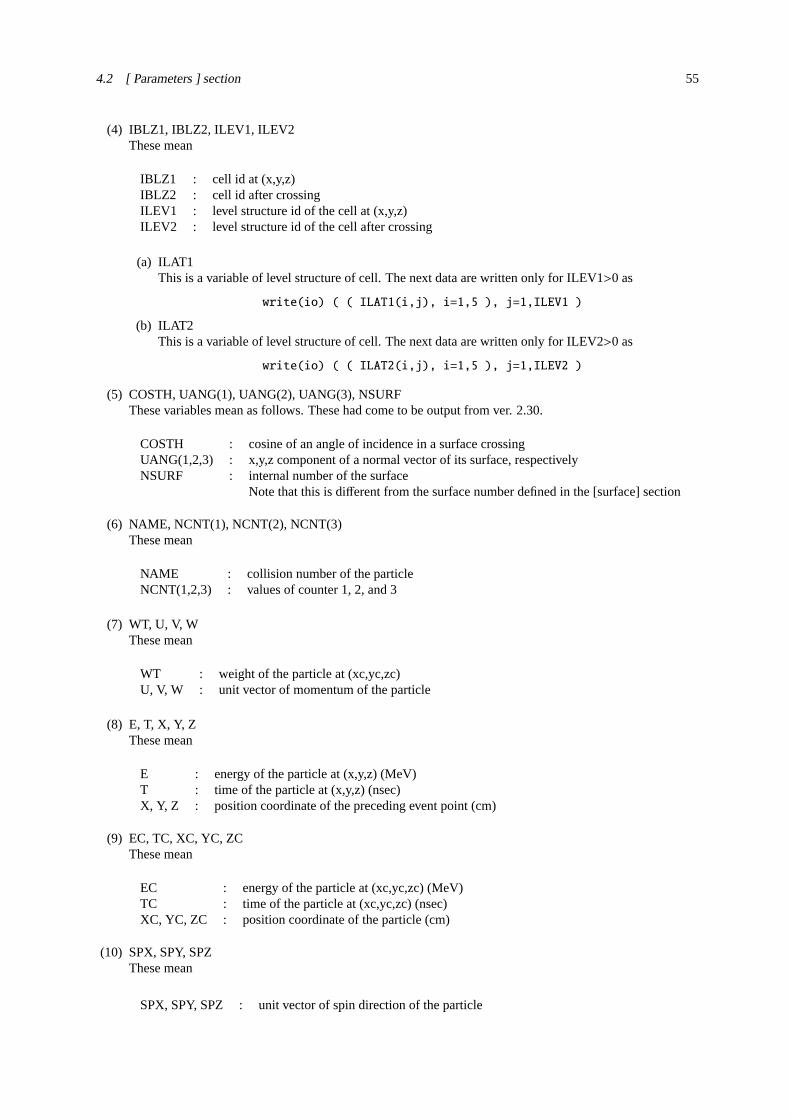
4.2 [ Parameters ] section 55
(4) IBLZ1, IBLZ2, ILEV1, ILEV2These mean
IBLZ1 : cell id at (x,y,z)IBLZ2 : cell id after crossingILEV1 : level structure id of the cell at (x,y,z)ILEV2 : level structure id of the cell after crossing
(a) ILAT1This is a variable of level structure of cell. The next data are written only for ILEV1>0 as
write(io) ( ( ILAT1(i,j), i=1,5 ), j=1,ILEV1 )
(b) ILAT2This is a variable of level structure of cell. The next data are written only for ILEV2>0 as
write(io) ( ( ILAT2(i,j), i=1,5 ), j=1,ILEV2 )
(5) COSTH, UANG(1), UANG(2), UANG(3), NSURFThese variables mean as follows. These had come to be output from ver. 2.30.
COSTH : cosine of an angle of incidence in a surface crossingUANG(1,2,3) : x,y,z component of a normal vector of its surface, respectivelyNSURF : internal number of the surface
Note that this is different from the surface number defined in the [surface] section
(6) NAME, NCNT(1), NCNT(2), NCNT(3)These mean
NAME : collision number of the particleNCNT(1,2,3) : values of counter 1, 2, and 3
(7) WT, U, V, WThese mean
WT : weight of the particle at (xc,yc,zc)U, V, W : unit vector of momentum of the particle
(8) E, T, X, Y, ZThese mean
E : energy of the particle at (x,y,z) (MeV)T : time of the particle at (x,y,z) (nsec)X, Y, Z : position coordinate of the preceding event point (cm)
(9) EC, TC, XC, YC, ZCThese mean
EC : energy of the particle at (xc,yc,zc) (MeV)TC : time of the particle at (xc,yc,zc) (nsec)XC, YC, ZC : position coordinate of the particle (cm)
(10) SPX, SPY, SPZThese mean
SPX, SPY, SPZ : unit vector of spin direction of the particle

56 4 SECTIONS FORMAT
(11) NZSTThis is charge state of the particle.
(12) NCLSTSThis variable is written only for NCOL=13, 14, collision case, and means the number of produced particleand nucleus. The next data are written for NCLSTS>0 case.
(a) MATHZ, MATHN, JCOLL, KCOLLThese mean
MATHZ : Z number of the mother nucleusMATHN : N number of the mother nucleusJCOLL : reaction type id1KCOLL : reaction type id2
JCOLL and KCOLL indicate the following meaning.
JCOLL0 : nothing happen1 : Hydrogen collisions2 : Particle Decays3 : Elastic collisions4 : High Energy Nuclear collisions5 : Heavy Ion reactions6 : Neutron reactions by data7 : Photon reactions by data8 : Electron reactions by data9 : Proton reactions by data
10 : Neutron event mode11 : delta ray production13 : Photon reactions by EGS514 : Electron reactions by EGS5
KCOLL0 : normal1 : high energy fission2 : high energy absorption3 : low energy n elastic4 : low energy n non-elastic5 : low energy n fission6 : low energy n absorption
(b) ICLUSTS, JCLUSTS, QCLUSTS, JCOUNTThese variables have a array and denote the information on the produced particle and nucleus.
do i = 1, NCLSTS
write(io) ICLUSTS(i)
write(io) ( JCLUSTS(j,i), j=0,7)
write(io) ( QCLUSTS(j,i), j=0,12)
write(io) ( JCOUNT(j,i), j=1,3)
end do
These mean

4.2 [ Parameters ] section 57
ICLUSTS kind of particle0 : nucleus1 : proton2 : neutron3 : pion4 : photon5 : kaon6 : muon7 : others
JCLUSTS(i)i = 0 : angular momentum= 1 : proton number= 2 : neutron number= 3 : ityp= 4 : status of the particle 0: real,<0 : dead= 5 : charge number= 6 : baryon number= 7 : kf code
QCLUSTS(i)i = 0 : impact parameter= 1 : px (GeV/c)= 2 : py (GeV/c)= 3 : pz (GeV/c)= 4 : etot =
√p2 +m2 (GeV)
= 5 : rest mass (GeV)= 6 : excitation energy (MeV)= 7 : kinetic energy (MeV)= 8 : weight= 9 : time (nsec)= 10 : x coordinate (cm)= 11 : y coordinate (cm)= 12 : z coordinate (cm)

58 4 SECTIONS FORMAT
4.2.22 Event Generator Mode
For Event Generator mode,35 36 37 one should define dmax(2) appropriately, since we need the informationfrom the data base as mentioned above. In the special statistical decay model, we use the detail information onthe level structure near the ground state for particle and photon emission. For this, we needigamma=1-3. Wehave developed the special statistical decay model based on GEM. Then one should need to specifynevap=3. Inthis mode, the effect of thermal motion of materials is not considered. It means that we always assumeT=0 in thismode. These parameters are automatically set if you specifye-mode=1 or 2 (unless explicitly specified,igamma=2is selected). For consistency reason, the combinationigamma=1 ande-mode=1 is also supported.
Event generator mode Ver.2 is the improved version of the legacy version (i.e. event generator mode Ver.1).In reactions emitting multiple neutrons, previous event generator mode samples the first ejectile neutron from thecross-section data and emission of the subsequent particles is simulated by the statistical decay model. While,ver.2 samples all the ejectile neutrons from the cross-section data and the statistical decay model is used merely tosimulate prompt gamma-ray production. As for capture reactions, previous event generator mode assumes that thetarget nucleus absorbs incident neutron and particle emission is simulated by the statistical decay model. In thiscase, ejectile particle species are fully determined by the statistical decay model. While ver.2 selects the ejectileparticle species depending on the reaction channel (i.e. in (n, α) reaction, emission of only one alpha particle andgamma-rays are allowed).
By this mode, we can obtain the following new observables, which cannot be detected without this mode. First,the deposition energy distribution in[t-heat] tally is available for low energy regime belowdmax(2). Second,in [t-yield] and[t-product], we can tally the yield and product quantities belowdmax(2). Third, the heatfrom neutrons is usually obtained from Kerma factors in the data base region. In this mode, the heat from neutronsis zero, but the heat is calculated from energy loss of all charged particles and nucleus. Fourth, DPA values isobtained even for the energy belowdmax(2) without DPA data base.
35 Y. Iwamotoet al., International Conference on Nuclear Data for Science and Technology 2007, DOI: 10.1051/ndata:07417.36 K. Niita et al., International Conference on Nuclear Data for Science and Technology 2007, DOI: 10.1051/ndata:07398.37 Y. Iwamotoet al., Prog. Nucl. Sci. Technol. 2, 931-935 (2011).
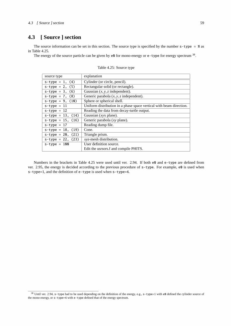
4.3 [ Source ] section 59
4.3 [ Source ] section
The source information can be set in this section. The source type is specified by the numbers-type = N asin Table4.25.
The energy of the source particle can be given bye0 for mono-energy ore-type for energy spectrum38.
Table 4.25:Source type
source type explanation
s-type = 1, (4) Cylinder (or circle, pencil).s-type = 2, (5) Rectangular solid (or rectangle).s-type = 3, (6) Gaussian (x, y, z independent).s-type = 7, (8) Generic parabola (x, y, z independent).s-type = 9, (10) Sphere or spherical shell.s-type = 11 Uniform distribution in a phase space vertical with beam direction.s-type = 12 Reading the data from decay-turtle output.s-type = 13, (14) Gaussian (xyx plane).s-type = 15, (16) Generic parabola (xyplane).s-type = 17 Reading dump file.s-type = 18, (19) Cone.s-type = 20, (21) Triangle prism.s-type = 22, (23) xyz-mesh distribution.s-type = 100 User definition source.
Edit the usrsors.f and compile PHITS.
Numbers in the brackets in Table4.25 were used until ver. 2.94. If bothe0 ande-type are defined fromver. 2.95, the energy is decided according to the previous procedure ofs-type. For example,e0 is used whens-type=1, and the definition ofe-type is used whens-type=4.
38 Until ver. 2.94,s-type had to be used depending on the definition of the energy, e.g.,s-type=1 with e0 defined the cylinder source ofthe mono-energy, ors-type=4 with e-type defined that of the energy spectrum.

60 4 SECTIONS FORMAT
4.3.1 <Source> : Multi-source
Using this multi-source function, plural sources specified bys-type can be defined. Each source begins with<source> = number, which defines the relative weights of the multi-sources.totfact = defines the globalnormalization. Note that<source> should not be written in the line following the line in whichreg parameter iswritten.
Table 4.26:Multi-source
parameter explanation
<source> = Defines a multi-source; the relative weight is defined by this number.totfact = (D=1) Global normalization factor.
If this is given by a positive number, the source particle is generated according to this ratio;if negative, the same particle is generated in each multi-source section with weights adjustedaccording to the ratio.
iscorr = (D=0) Multi-source correlation option.0: Normal multi-source.1: Correlated multi-source. In this case, sources from each multi-source group are generatedas an event. This option is useful for estimating detector response by nuclear reactions pro-ducing several secondary particles. Note that the locations of all sources generated in an eventare not the same, unlike the case ofiscorr = 2,3.2: Correlated multi-source. In this case, the locations of all sources generated in an eventare the same. This mode is useful for simulating a nuclear reaction occurring at an arbitrarylocation.3: Correlated multi-source. In this case, the locations of all sources generated in an event arethe same, and the direction of the second source is opposite to that of the first. This mode isuseful for simulating a particle decaying into two particles at an arbitrary location.
The multiplicity of each source must be specified as an integer value representing its<source> parameter, and the sum of the multiplicities must be specified as thetotfact
parameter. For example, to simulate (X,1p2n) reaction as an event, set<source>=1 and 2 forproton and neutron sources, respectively, andtotfact=3.

4.3 [ Source ] section 61
4.3.2 Common parameters
Common parameters for each source type are shown below. The order of the parameters in the source section isfree. If a parameter has a default value (D=***), it can be omitted. The energies ofd, t, α, and nuclei are specifiedby [MeV/nucleon].
Table 4.27:Common source parameters (1)
parameter explanation
proj = Projectile: see Table3.4for specification.sx = (D=0) x-component of spin.sy = (D=0) y-component of spin.sz = (D=0) z-component of spin.reg = (D=all) The source region can be restricted within overlaps between regions defined by each
s-type and those specified by this parameter. The format isreg = 1 - 5 10 34. Thelattice and universe frame can be used asreg = ( 6 < 10[1 0 0] < u=3 ). See section ontally region specification for more detail.
ntmax = (D=1000) Maximum re-try number whenreg is specified.trcl = (D=none) Transform number, or definition of transform.wgt = (D=1.0) Weight of source particle.factor = (D=1.0) Normalization factor of source particle. PHITS multiplies all results of tally byfactor.
When using multi-source,totfact should be used instead offactor; when not using multi-source,totfact * factor is an actual normalization factor.
izst = (D=charge of particle specified withproj=) Charge state of source particle.This has an effect only on motion in the magnetic and electric fields defined in[magneticfield] and[electro magnetic field] sections, respectively.The charge number defined withizst doesn’t change while the particle moves. Note that particlesproduced from nuclear reactions are not affected by the value ofizst; the charge of the producedparticle is given as its atomic number.
θ
z
xy
cosθ=dir
φ=phi
ψ=dom
Figure 4.2:Source direction and parame-tersdir, phi, dom.
The projectile direction is specified by three parameters:dir,phi, anddom. The relation between these is shown in Fig.4.2, inwhich the direction is noted as a thick arrow.dir is the directioncosine relative to thez axis. phi is the azimuthal angle from thex axis and is given in degrees; if not set by the user, the value ofthe azimuthal cosine is selected randomly. Using the parameterdom
spreads the direction determined bydir andphi by the solid angle2π(1− cosψ), whereψ = dom (in degrees). In the PHITS calculation,the angle is selected randomly within the solid angle.
By settingdir=all, the direction of the source beam becomesisotropic. To use a specific angular distribution, a subsection in thedistribution based on numerical data or an analytic function startingfrom a-type is required.
In s-type=9, the definition ofdir differs. Ins-type=11 and12, dir can only bet set= −1 or 1.
To transform coordinates, thetrcl parameter, which specifiesthe transform number or the definition of the transformation itself,can be used. The relation ofwgt andfactor is reciprocal.
If its spin is not defined or zero, a neutron enters a magnetic field without spin. In this case, the initial spinof the neutron is determined at the entrance of the magnetic field by the direction of the magnetic field and thepolarization factor. If the spin is defined in this section, the neutron enters the magnetic field with the defined spindirection irrespective of the direction of the magnetic field and polarization.

62 4 SECTIONS FORMAT
Table 4.28:Common source parameters (2)
parameter explanation
ispfs = 0, 1, 2 (D=0) Neutron sources from spontaneous fission.If ispfs=1 or 2 is specified in the[source] section and the following 18 nuclei arechosen asproj, neutrons can be defined using spontaneous fission as a source. Thesenuclei are assumed to be spontaneous fission nuclei:U-238, Pu-238, Pu-240, Pu-242, Cm-242, Cm-244, Cf-252, Th-232, U-232, U-233, U-234, U-235, U-236, Np-237, Pu-239, Pu-241, Am-241, Bk-249.ispfs=1: Tally result is normalized by the number of neutrons produced by spontaneousfission.ispfs=2: Tally result is normalized by the number of spontaneous fissions.In the case ofispfs = 1,2, e0 ande-type, dir, anda-type are neglected.
Whenispfs=1,2 is specified, the multiplicity and energy spectrum of neutrons are taken from the reference39.The PHITS development team is grateful to Dr. Liem Peng Hong of NAIS, Co., Inc. for his support in developingthis function to generate neutron sources.
In the next example, settingproj=240Pu andispfs=1 selects neutrons from the spontaneous fission of Pu-240as source particles. In this case, the value ofe0 is invalid.
[ S o u r c e ]
s-type = 1
proj = 240Pu
e0 = 1.0
z0 = 0
z1 = 0
r0 = 0.0
dir = 1.0000
ispfs = 1
39 J. M. Verbeke, C. Hagmnn, and D. Wright, “Simulation of Neutron and Gamma Ray Emission from Fission and Photofission”, UCRL-AR-228518 (2014).

4.3 [ Source ] section 63
4.3.3 Cylinder distribution source
Parameters for cylinder source are shown below. The order of parameters is free. If a parameter has a defaultvalue (D=***), the parameter can be omissible.
Table 4.29:Parameters for cylinder source
s-type = 1 Cylinder or circle source.x0 = (D=0.0) x coordinate of center position of cylinder source[cm].y0 = (D=0.0)y coordinate of center position of cylinder source[cm].z0 = (D=0.0) Minimumzof cylinder source[cm].z1 = (D=0.0) Maximumz of cylinder source[cm], (when z1=z0, circle plane source).r0 = (D=0.0) Radius of cylinder source, (whenr0=0.0, pencil source)[cm].r1 = (D=0.0) Inner radius for inner void of cylinder.dir = (D=1.0) Direction cosine of projectile againstzaxis.
If you setall, it is isotropic.If you setdata, a-type subsection is necessary.
phi = (D=none; random) Azimuthal angle[degree].dom = (D=0.0) Solid angle[degree].
= −1 ; cos2 bias distribution.e0 = (For mono-energy) Projectile energy[MeV/u].
e-type = (For energy spectrum) Projectile energy[MeV/u].
4.3.4 Rectangular solid distribution source
Parameters for rectangular solid source are shown below. The order of parameters is free. If a parameter has adefault value (D=***), the parameter can be omissible.
Table 4.30:Parameters for rectangular solid source
s-type = 2 Rectangular solid and rectangle source.x0 = (D=0.0) Minimumx coordinate[cm].x1 = (D=0.0) Maximumx coordinate[cm].y0 = (D=0.0) Minimumy coordinate[cm].y1 = (D=0.0) Maximumy coordinate[cm].z0 = (D=0.0) Minimumz coordinate[cm].z1 = (D=0.0) Maximumz coordinate[cm], when (z1=z0), rectangle source.dir = (D=1.0) Direction cosine of projectile againstzaxis.
If you setall, it is isotropic.If you setdata, a-type subsection is necessary.
phi = (D=none; random) Azimuthal angle[degree].dom = (D=0.0) Solid angle[degree].
= −1 ; cos2 bias distribution.e0 = (For mono-energy) Projectile energy[MeV/u].
e-type = (For energy spectrum) Projectile energy[MeV/u].

64 4 SECTIONS FORMAT
4.3.5 Gaussian distribution source (x,y,z independent)
This Gauss distribution is consist of independent Gaussian in each x, y, z direction. Parameters for Gaussiansource are shown below. The order of parameters is free. If a parameter has a default value (D=***), the parametercan be omissible.
Table 4.31:Parameters for Gaussian source
s-type = 3 Gaussian source.x0 = (D=0.0) x coordinate of Gaussian center[cm].x1 = (D=0.0) FWHM in x direction[cm].y0 = (D=0.0)y coordinate of Gaussian center[cm].y1 = (D=0.0) FWHM iny direction[cm].z0 = (D=0.0)z coordinate of Gaussian center[cm].z1 = (D=0.0) FWHM inzdirection[cm].dir = (D=1.0) Direction cosine of projectile againstz axis.
If you setall, it is isotropic.If you setdata, a-type subsection is necessary.
phi = (D=none; random) Azimuthal angle[degree].dom = (D=0.0) Solid angle[degree].
= −1 ; cos2 bias distribution.e0 = (For mono-energy) Projectile energy[MeV/u].
e-type = (For energy spectrum) Projectile energy[MeV/u].
4.3.6 Generic parabola distribution source (x,y,z independent)
This generic parabola distribution consists of independent parabola in each x, y, z direction. Parameters forgeneric parabola source are shown below. The order of parameters is free. If a parameter has a default value(D=***), the parameter can be omissible.
Table 4.32:parameters for generic parabola distribution
s-type = 7 Generic parabola source.x0 = (D=0.0) x coordinate of X-parabola center[cm].x1 = (D=0.0) X-parabola width[cm].y0 = (D=0.0)y coordinate of Y-parabola center[cm].y1 = (D=0.0) Y-parabola width[cm].z0 = (D=0.0) Minimumz of parabola[cm].z1 = (D=0.0) Maximumzof parabola[cm].rn = (D=2) Order of generic parabola.dir = (D=1.0) Direction cosine of projectile againstz axis.
If you setall, it is isotropic.If you setdata, a-type subsection is necessary.
phi = (D=none; random) Azimuthal angle[degree].dom = (D=0.0) Solid angle[degree].
= −1 ; cos2 bias distribution.e0 = (For mono-energy) Projectile energy[MeV/u].
e-type = (For energy spectrum) Projectile energy[MeV/u].
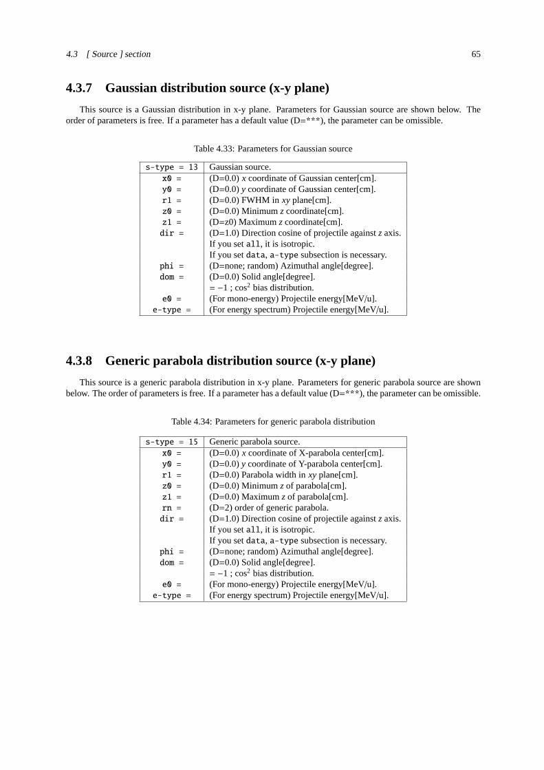
4.3 [ Source ] section 65
4.3.7 Gaussian distribution source (x-y plane)
This source is a Gaussian distribution in x-y plane. Parameters for Gaussian source are shown below. Theorder of parameters is free. If a parameter has a default value (D=***), the parameter can be omissible.
Table 4.33:Parameters for Gaussian source
s-type = 13 Gaussian source.x0 = (D=0.0) x coordinate of Gaussian center[cm].y0 = (D=0.0)y coordinate of Gaussian center[cm].r1 = (D=0.0) FWHM in xyplane[cm].z0 = (D=0.0) Minimumzcoordinate[cm].z1 = (D=z0) Maximumz coordinate[cm].dir = (D=1.0) Direction cosine of projectile againstzaxis.
If you setall, it is isotropic.If you setdata, a-type subsection is necessary.
phi = (D=none; random) Azimuthal angle[degree].dom = (D=0.0) Solid angle[degree].
= −1 ; cos2 bias distribution.e0 = (For mono-energy) Projectile energy[MeV/u].
e-type = (For energy spectrum) Projectile energy[MeV/u].
4.3.8 Generic parabola distribution source (x-y plane)
This source is a generic parabola distribution in x-y plane. Parameters for generic parabola source are shownbelow. The order of parameters is free. If a parameter has a default value (D=***), the parameter can be omissible.
Table 4.34:Parameters for generic parabola distribution
s-type = 15 Generic parabola source.x0 = (D=0.0) x coordinate of X-parabola center[cm].y0 = (D=0.0)y coordinate of Y-parabola center[cm].r1 = (D=0.0) Parabola width inxyplane[cm].z0 = (D=0.0) Minimumzof parabola[cm].z1 = (D=0.0) Maximumz of parabola[cm].rn = (D=2) order of generic parabola.dir = (D=1.0) Direction cosine of projectile againstzaxis.
If you setall, it is isotropic.If you setdata, a-type subsection is necessary.
phi = (D=none; random) Azimuthal angle[degree].dom = (D=0.0) Solid angle[degree].
= −1 ; cos2 bias distribution.e0 = (For mono-energy) Projectile energy[MeV/u].
e-type = (For energy spectrum) Projectile energy[MeV/u].

66 4 SECTIONS FORMAT
4.3.9 Sphere and spherical shell distribution source
Parameters for sphere and spherical shell sources are shown below. The order of parameters is free. If aparameter has a default value (D=***), the parameter can be omitted.
Table 4.35:Parameters for sphere and spherical shell source
s-type = 9 Sphere and spherical shell source.x0 = (D=0.0) x coordinate of sphere center[cm].y0 = (D=0.0)y coordinate of sphere center[cm].z0 = (D=0.0)z coordinate of sphere center[cm].r1 = (D=0.0) Inside radius[cm]. Ifr1=0, sphere source.r2 = (D=0.0) Outside radius[cm].dir = (D=1.0) Direction.
dir = 1.0 : Outgoing from the center with normal line direction.dir = -1.0 : Inverse direction withdir=1.0.dir = all : Isotropic.dir = -all : Inverse direction againstdir=1.0, and with cosine distribution. This is usedfor volume and area calculation with cos2 bias.dir=iso : Uniform distribution on a circle of radiusr2 on a spherical shell of radiusr1 withthe direction orthogonal to a circle of radiusr2 toward the sphere. In the case ofr1=r2, theresult is nearly identical to that ofdir = -all, but the effect of weight is not included. Thus,this condition can be used to obtain the variance of deposition energies on the[t-deposit]
tally with output=deposit.e0 = (For mono-energy) Projectile energy[MeV/u].
e-type = (For energy spectrum) Projectile energy[MeV/u].
When using the source types-type=9 for volume and area calculation, setdir=-all, r1=r2; dir=isogives the same result.
Inner radius,r1, should be smaller or equal to outer radius,r2, except fordir=iso, wherer1 should be equalto (or larger than)r2.
r2
r1
Figure 4.3: Schematic of the source in the case ofdir=iso.
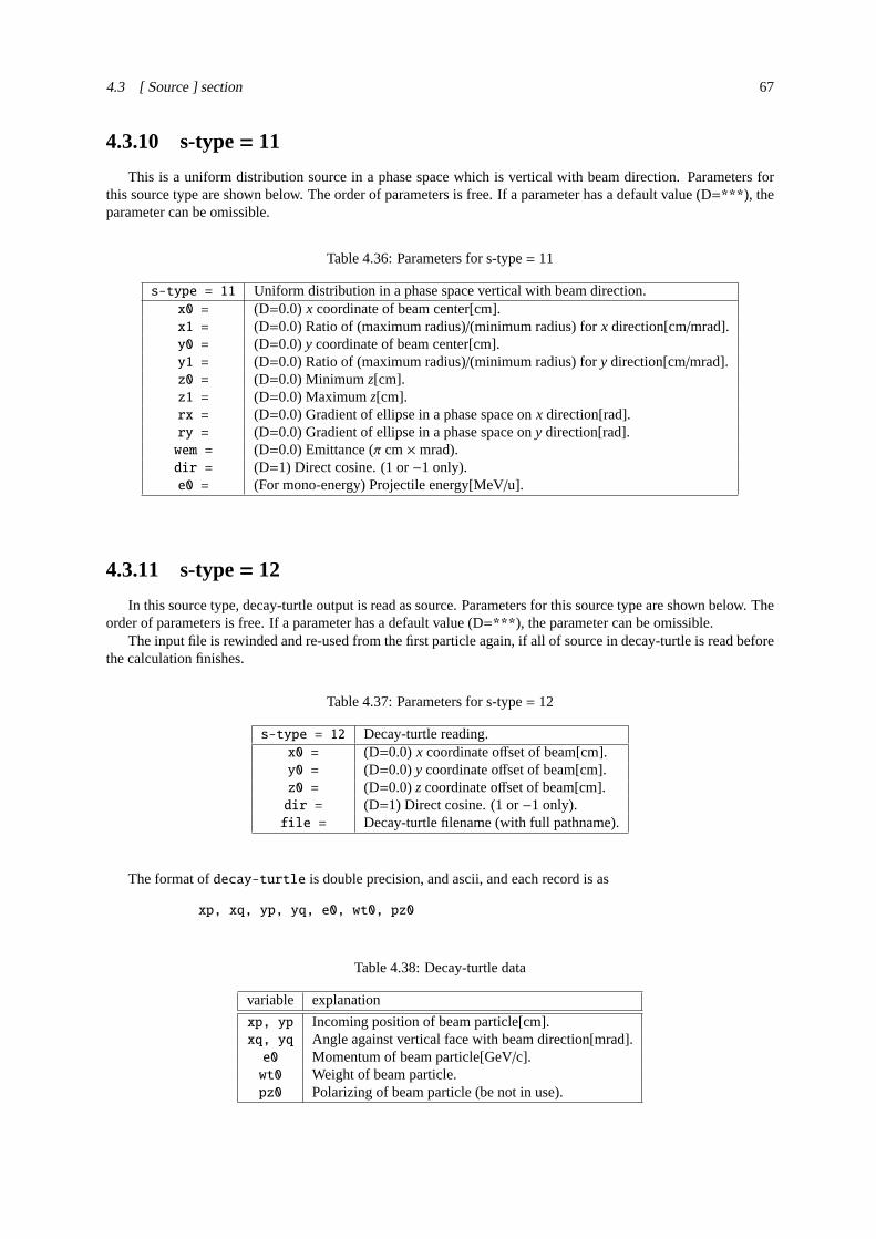
4.3 [ Source ] section 67
4.3.10 s-type= 11
This is a uniform distribution source in a phase space which is vertical with beam direction. Parameters forthis source type are shown below. The order of parameters is free. If a parameter has a default value (D=***), theparameter can be omissible.
Table 4.36:Parameters for s-type= 11
s-type = 11 Uniform distribution in a phase space vertical with beam direction.x0 = (D=0.0) x coordinate of beam center[cm].x1 = (D=0.0) Ratio of (maximum radius)/(minimum radius) forx direction[cm/mrad].y0 = (D=0.0)y coordinate of beam center[cm].y1 = (D=0.0) Ratio of (maximum radius)/(minimum radius) fory direction[cm/mrad].z0 = (D=0.0) Minimumz[cm].z1 = (D=0.0) Maximumz[cm].rx = (D=0.0) Gradient of ellipse in a phase space onx direction[rad].ry = (D=0.0) Gradient of ellipse in a phase space ony direction[rad].wem = (D=0.0) Emittance (π cm×mrad).dir = (D=1) Direct cosine. (1 or−1 only).e0 = (For mono-energy) Projectile energy[MeV/u].
4.3.11 s-type= 12
In this source type, decay-turtle output is read as source. Parameters for this source type are shown below. Theorder of parameters is free. If a parameter has a default value (D=***), the parameter can be omissible.
The input file is rewinded and re-used from the first particle again, if all of source in decay-turtle is read beforethe calculation finishes.
Table 4.37:Parameters for s-type= 12
s-type = 12 Decay-turtle reading.x0 = (D=0.0) x coordinate offset of beam[cm].y0 = (D=0.0)y coordinate offset of beam[cm].z0 = (D=0.0)z coordinate offset of beam[cm].dir = (D=1) Direct cosine. (1 or−1 only).file = Decay-turtle filename (with full pathname).
The format ofdecay-turtle is double precision, and ascii, and each record is as
xp, xq, yp, yq, e0, wt0, pz0
Table 4.38:Decay-turtle data
variable explanation
xp, yp Incoming position of beam particle[cm].xq, yq Angle against vertical face with beam direction[mrad].e0 Momentum of beam particle[GeV/c].wt0 Weight of beam particle.pz0 Polarizing of beam particle (be not in use).

68 4 SECTIONS FORMAT
4.3.12 Cone shape
Parameters for cone shape source are shown below. The order of parameters is free. If a parameter has a defaultvalue (D=***), the parameter can be omissible.
Table 4.39:parameters for cone shape
s-type = 18 Cone shape.x0 = (D=0.0) x coordinate offset of top of cone[cm].y0 = (D=0.0)y coordinate offset of top of cone[cm].z0 = (D=0.0)z coordinate offset of top of cone[cm].x1 = (D=0.0) x-component of vector from top to center of bottom circle[cm].y1 = (D=0.0)y-component of vector from top to center of bottom circle[cm].z1 = (D=0.0)z-component of vector from top to center of bottom circle[cm].r0 = (D=0.0) distance between top and upper end of source locations on axis of cone[cm].r1 = (D=0.0) Distance between top and lower end of source locations on axis of cone[cm].r2 = (D=0.0) Angle between generatrix and axis of cone[degree].dir = (D=1.0) Direction cosine of projectile againstzaxis.
If you setall, it is isotropic.If you setdata, a-type subsection is necessary.
phi = (D=none; random) Azimuthal angle[degree].dom = (D=0.0) Solid angle[degree].
= −1 ; cos2 bias distribution.e0 = (For mono-energy) Projectile energy[MeV/u].
e-type = (For energy spectrum) Projectile energy[MeV/u].

4.3 [ Source ] section 69
4.3.13 Triangle prism shape
Parameters for triangle prism shape source are shown below. The order of parameters is free. If a parameterhas a default value (D=***), the parameter can be omissible.
Table 4.40:parameters for triangle prism shape
s-type = 20 Triangle prism shape.x0 = (D=0.0) x-coordinate of origin apex of triangle[cm].y0 = (D=0.0)y-coordinate of origin apex of triangle[cm].z0 = (D=0.0)z-coordinate of origin apex of triangle[cm].x1 = (D=0.0) x vector from the origin to the first apex[cm].y1 = (D=0.0)y vector from the origin to the first apex[cm].z1 = (D=0.0)z vector from the origin to the first apex[cm].x2 = (D=0.0) x vector from the origin to the second apex[cm].y2 = (D=0.0)y vector from the origin to the second apex[cm].z2 = (D=0.0)z vector from the origin to the second apex[cm].x3 = (D=0.0) x vector from the origin to the third apex[cm].y3 = (D=0.0)y vector from the origin to the third apex[cm].z3 = (D=0.0)z vector from the origin to the third apex[cm].exa = (D=0.0) Attenuation coefficient. exa>0; exp (−ax), exa=0; uniform.dir = (D=1.0) Direction cosine of projectile againstz axis.
If you setall, it is isotropic.If you setdata, a-type subsection is necessary.
phi = (D=none; random) Azimuthal angle[degree].dom = (D=0.0) Solid angle[degree].
= −1 ; cos2 bias distribution.e0 = (For mono-energy) Projectile energy[MeV/u].
e-type = (For energy spectrum) Projectile energy[MeV/u].
Figure 4.4:Coordinates of triangle prism

70 4 SECTIONS FORMAT
4.3.14 xyz-mesh distribution source
When you specifys-type=22, you can set a complex spatial distribution of sources. Instype=22, mono-energetic particles can be generated. The spatial distribution can be defined byx,y,z-type subsections and dataof relative intensitiesI i jk , (i = 1, · · · ,nx; j = 1, · · · ,ny; k = 1, · · · ,nz). The data should be written below thesubsections. The direction of the sources can be specified bydir, phi, anddom. Note that you cannot changethe direction in each xyz-bin. Parameters for xyz-mesh distribution source are shown in Table4.41. The order ofparameters is free except for the data of the relative intensities. If a parameter has a default value (D=***), theparameter can be omissible.
Table 4.41:parameters for xyz-mesh distribution source
s-type = 22 xyz-mesh distribution source.mesh = xyz Geometry mesh. Onlyxyz can be set.x-type = Mesh type forx-axis.x-type subsection is needed below this option.y-type = Mesh type fory-axis.y-type subsection is needed below this option.z-type = Mesh type forz-axis.z-type subsection is needed below this option.
Put data of relative intensitiesI i jk below x, y, z-type subsections. The change of thedata element should be in the order ofx, y, z. Note that the change inx, y, z axes should beascending order ifnx, ny, nz are positive, and it should be descending order ifnx, ny,nz are negative.
dir = (D=1.0) Direction cosine of projectile againstz axis.If you setall, it is isotropic.If you setdata, a-type subsection is necessary.
phi = (D=none; random) Azimuthal angle[degree].dom = (D=0.0) Solid angle[degree].
= −1 ; cos2 bias distribution.e0 = (For mono-energy) Projectile energy[MeV/u].
e-type = (For energy spectrum) Projectile energy[MeV/u].
When all ofnx,ny,nz are positive, the order of the relative intensitiesI i jk is given as
I111, I211, · · · , Inx11, I121, I221, · · · , Inxny1, I112, I212, · · · , Inxnynz, (2)
wherenx =|nx|, ny =|ny|, nz =|nz|. Whennx andny are positive andnz is negative, the order is given as
I11nz, I21nz, · · · , Inx1nz, I12nz, I22nz, · · · , Inxnynz, I11nz−1, I21nz−1, · · · , Inxny1. (3)
In the latter case, you have to first put the data withk = nz =|nz|.An example usings-type=22 is shown below.
Example 3: Example of xyz-mesh distribution source
1: [ S o u r c e ]
2: s-type = 22
3: proj = neutron
4: e0 = 1.0
5: dir = all
6: mesh = xyz
7: x-type = 2
8: nx = 3
9: xmin = -10
10: xmax = 10
11: y-type = 2
12: ny = -3
13: ymin = -10
14: ymax = 10
15: z-type = 2
16: nz = -2
17: zmin = -10
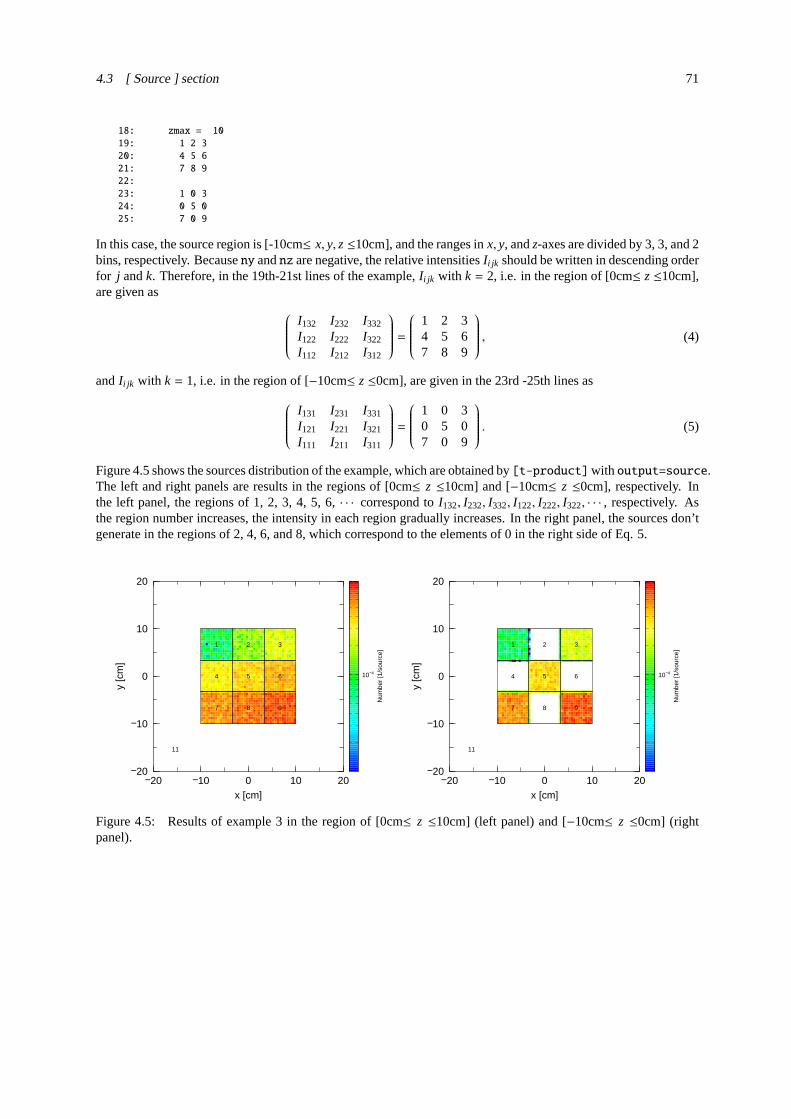
4.3 [ Source ] section 71
18: zmax = 10
19: 1 2 3
20: 4 5 6
21: 7 8 9
22:
23: 1 0 3
24: 0 5 0
25: 7 0 9
In this case, the source region is [-10cm≤ x, y, z≤10cm], and the ranges inx, y, andz-axes are divided by 3, 3, and 2bins, respectively. Becauseny andnz are negative, the relative intensitiesI i jk should be written in descending orderfor j andk. Therefore, in the 19th-21st lines of the example,I i jk with k = 2, i.e. in the region of [0cm≤ z≤10cm],are given as I132 I232 I332
I122 I222 I322
I112 I212 I312
= 1 2 3
4 5 67 8 9
, (4)
andI i jk with k = 1, i.e. in the region of [−10cm≤ z≤0cm], are given in the 23rd -25th lines as I131 I231 I331
I121 I221 I321
I111 I211 I311
= 1 0 3
0 5 07 0 9
. (5)
Figure4.5shows the sources distribution of the example, which are obtained by[t-product]with output=source.The left and right panels are results in the regions of [0cm≤ z ≤10cm] and [−10cm≤ z ≤0cm], respectively. Inthe left panel, the regions of 1, 2, 3, 4, 5, 6,· · · correspond toI132, I232, I332, I122, I222, I322, · · · , respectively. Asthe region number increases, the intensity in each region gradually increases. In the right panel, the sources don’tgenerate in the regions of 2, 4, 6, and 8, which correspond to the elements of 0 in the right side of Eq.5.
−20 −10 0 10 20−20
−10
0
10
20
x [cm]
y [c
m]
11
7 8 9
4 5 6
1 2 3
10−4
Num
ber
[1/s
ourc
e]
−20 −10 0 10 20−20
−10
0
10
20
x [cm]
y [c
m]
11
7 8 9
4 5 6
1 2 3
10−4N
umbe
r [1
/sou
rce]
Figure 4.5: Results of example3 in the region of [0cm≤ z ≤10cm] (left panel) and [−10cm≤ z ≤0cm] (rightpanel).
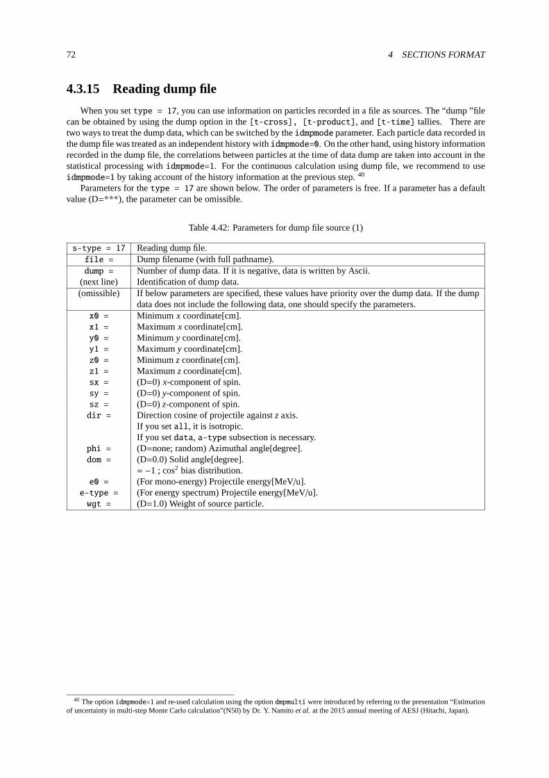
72 4 SECTIONS FORMAT
4.3.15 Reading dump file
When you settype = 17, you can use information on particles recorded in a file as sources. The “dump ”filecan be obtained by using the dump option in the[t-cross], [t-product], and[t-time] tallies. There aretwo ways to treat the dump data, which can be switched by theidmpmode parameter. Each particle data recorded inthe dump file was treated as an independent history withidmpmode=0. On the other hand, using history informationrecorded in the dump file, the correlations between particles at the time of data dump are taken into account in thestatistical processing withidmpmode=1. For the continuous calculation using dump file, we recommend to useidmpmode=1 by taking account of the history information at the previous step.40
Parameters for thetype = 17 are shown below. The order of parameters is free. If a parameter has a defaultvalue (D=***), the parameter can be omissible.
Table 4.42:Parameters for dump file source (1)
s-type = 17 Reading dump file.file = Dump filename (with full pathname).dump = Number of dump data. If it is negative, data is written by Ascii.
(next line) Identification of dump data.(omissible) If below parameters are specified, these values have priority over the dump data. If the dump
data does not include the following data, one should specify the parameters.x0 = Minimum x coordinate[cm].x1 = Maximumx coordinate[cm].y0 = Minimum y coordinate[cm].y1 = Maximumy coordinate[cm].z0 = Minimum zcoordinate[cm].z1 = Maximumzcoordinate[cm].sx = (D=0) x-component of spin.sy = (D=0) y-component of spin.sz = (D=0) z-component of spin.dir = Direction cosine of projectile againstz axis.
If you setall, it is isotropic.If you setdata, a-type subsection is necessary.
phi = (D=none; random) Azimuthal angle[degree].dom = (D=0.0) Solid angle[degree].
= −1 ; cos2 bias distribution.e0 = (For mono-energy) Projectile energy[MeV/u].
e-type = (For energy spectrum) Projectile energy[MeV/u].wgt = (D=1.0) Weight of source particle.
40 The optionidmpmode=1 and re-used calculation using the optiondmpmulti were introduced by referring to the presentation “Estimationof uncertainty in multi-step Monte Carlo calculation”(N50) by Dr. Y. Namitoet al. at the 2015 annual meeting of AESJ (Hitachi, Japan).
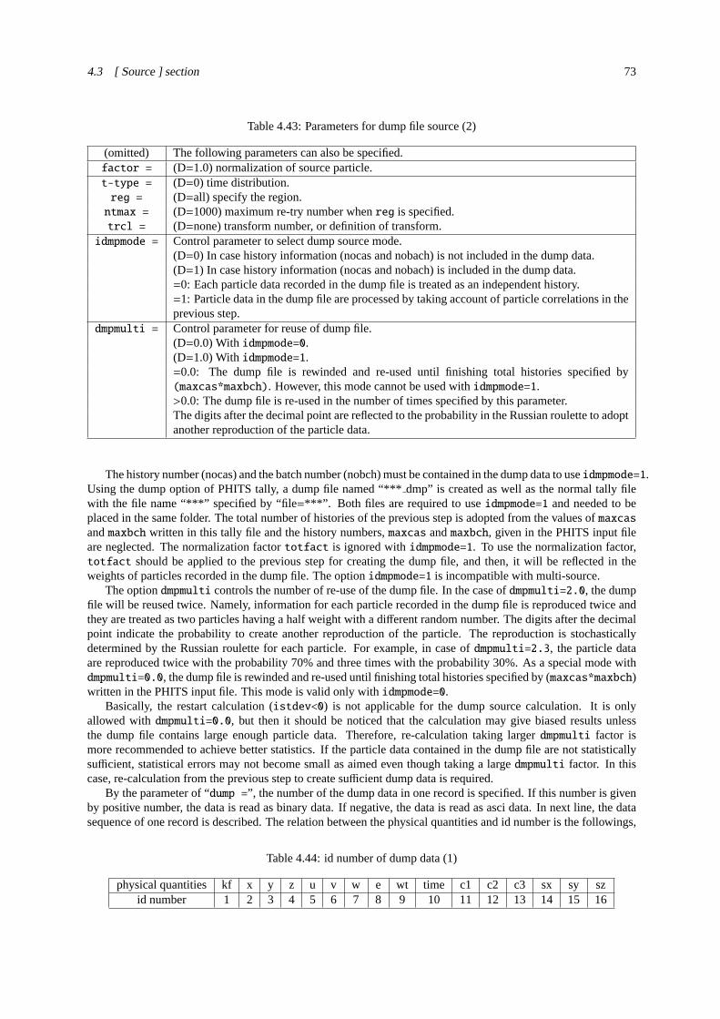
4.3 [ Source ] section 73
Table 4.43:Parameters for dump file source (2)
(omitted) The following parameters can also be specified.factor = (D=1.0) normalization of source particle.t-type = (D=0) time distribution.reg = (D=all) specify the region.ntmax = (D=1000) maximum re-try number whenreg is specified.trcl = (D=none) transform number, or definition of transform.
idmpmode = Control parameter to select dump source mode.(D=0) In case history information (nocas and nobach) is not included in the dump data.(D=1) In case history information (nocas and nobach) is included in the dump data.=0: Each particle data recorded in the dump file is treated as an independent history.=1: Particle data in the dump file are processed by taking account of particle correlations in theprevious step.
dmpmulti = Control parameter for reuse of dump file.(D=0.0) Withidmpmode=0.(D=1.0) Withidmpmode=1.=0.0: The dump file is rewinded and re-used until finishing total histories specified by(maxcas*maxbch). However, this mode cannot be used withidmpmode=1.>0.0: The dump file is re-used in the number of times specified by this parameter.The digits after the decimal point are reflected to the probability in the Russian roulette to adoptanother reproduction of the particle data.
The history number (nocas) and the batch number (nobch) must be contained in the dump data to useidmpmode=1.Using the dump option of PHITS tally, a dump file named “***dmp” is created as well as the normal tally filewith the file name “***” specified by “file=***”. Both files are required to useidmpmode=1 and needed to beplaced in the same folder. The total number of histories of the previous step is adopted from the values ofmaxcas
andmaxbch written in this tally file and the history numbers,maxcas andmaxbch, given in the PHITS input fileare neglected. The normalization factortotfact is ignored withidmpmode=1. To use the normalization factor,totfact should be applied to the previous step for creating the dump file, and then, it will be reflected in theweights of particles recorded in the dump file. The optionidmpmode=1 is incompatible with multi-source.
The optiondmpmulti controls the number of re-use of the dump file. In the case ofdmpmulti=2.0, the dumpfile will be reused twice. Namely, information for each particle recorded in the dump file is reproduced twice andthey are treated as two particles having a half weight with a different random number. The digits after the decimalpoint indicate the probability to create another reproduction of the particle. The reproduction is stochasticallydetermined by the Russian roulette for each particle. For example, in case ofdmpmulti=2.3, the particle dataare reproduced twice with the probability 70% and three times with the probability 30%. As a special mode withdmpmulti=0.0, the dump file is rewinded and re-used until finishing total histories specified by (maxcas*maxbch)written in the PHITS input file. This mode is valid only withidmpmode=0.
Basically, the restart calculation (istdev<0) is not applicable for the dump source calculation. It is onlyallowed withdmpmulti=0.0, but then it should be noticed that the calculation may give biased results unlessthe dump file contains large enough particle data. Therefore, re-calculation taking largerdmpmulti factor ismore recommended to achieve better statistics. If the particle data contained in the dump file are not statisticallysufficient, statistical errors may not become small as aimed even though taking a largedmpmulti factor. In thiscase, re-calculation from the previous step to create sufficient dump data is required.
By the parameter of “dump =”, the number of the dump data in one record is specified. If this number is givenby positive number, the data is read as binary data. If negative, the data is read as asci data. In next line, the datasequence of one record is described. The relation between the physical quantities and id number is the followings,
Table 4.44:id number of dump data (1)
physical quantities kf x y z u v w e wt time c1 c2 c3 sx sy szid number 1 2 3 4 5 6 7 8 9 10 11 12 13 14 15 16

74 4 SECTIONS FORMAT
Table 4.45:id number of dump data (2)
physical quantities name nocas nobch noid number 17 18 19 20
Here kf means the kf-code of the particles (see Table3.4), x, y, z are coordinates[cm]., u, v, w denote the unitvectors of the direction of the particle, e is the energy (MeV, or MeV/nucleon for nucleus), wt is the weight, timeis the initial time (ns), c1, c2, c3 are the values of counters, and sx, sy, sz are the unit vectors of the direction ofspin, respectively. name is a collision number of the particle, nocas is a history number of a batch, nobch is abatch number, no is a cascade id in the history. These are assumed as real*8 for the binary data,n(1p1e24.15) dataformat for the ascii data.
For an example, one record has 9 data as
kf e wt x y z u v w
To read this data, we write the parameters as
dump = 9
1 8 9 2 3 4 5 6 7

4.3 [ Source ] section 75
4.3.16 User definition source
If you edit usrsors.f, you can use your original source function by s-type=100. If the following parameters areset, these values have the priority. If a parameter has a default value (D=***), the parameter can be omissible.
Table 4.46:Parameters can be specified in s-type=100
s-type = 100 User definition source.If below parameters are specified, these values have priority over the user defined data.
x0 = Minimum x coordinate[cm].x1 = Maximumx coordinate[cm].y0 = Minimum y coordinate[cm].y1 = Maximumy coordinate[cm].z0 = Minimum zcoordinate[cm].z1 = Maximumz coordinate[cm].sx = (D=0) x-component of spin.sy = (D=0) y-component of spin.sz = (D=0) z-component of spin.dir = Direction cosine of projectile againstz axis.
If you setall, it is isotropic.If you setdata, a-type subsection is necessary.
phi = (D=none; random) Azimuthal angle[degree].dom = (D=0.0) Solid angle[degree].
= −1 ; cos2 bias distribution.e0 = (For mono-energy) Projectile energy[MeV/u].
e-type = (For energy spectrum) Projectile energy[MeV/u].wgt = (D=1.0) Weight of source particle.factor = (D=1.0) Normalization of source particle.t-type = (D=0) Time distribution.reg = (D=all) Specify the region.ntmax = (D=1000) Maximum re-try number whenreg is specified.trcl = (D=none) Transform number, or definition of transform.

76 4 SECTIONS FORMAT
We show a sample program of usrsors.f as following. In the first comment part, there is a list of the variableswhich is necessary to define the source. Next there is a list of kf-code which specifies the source particle. In thelast part of the comment, the random number functions, one is a uniform random number, the other is a Gaussianrandom number, are shown. The first part of the program is an example of the initialization, which describes theopen and close the data file. The remaining part shows a list of the variables which user should define in thissubroutine.
File 2: usrsors.f
1: ************************************************************************
2: subroutine usrsors(x,y,z,u,v,w,e,wt,time,name,kf,nc1,nc2,nc3,
3: & sx,sy,sz)
4: * sample subroutine for user defined source. *
5: * variables : *
6: * x, y, z : position of the source. *
7: * u, v, w : unit vector of the particle direction. *
8: * e : kinetic energy of particle (MeV). *
9: * wt : weight of particle. *
10: * time : initial time of particle. (ns) *
11: * name : usually = 1, for Coulmb spread. *
12: * kf : kf code of the particle. *
13: * nc1 : initial value of counter 1 *
14: * nc2 : initial value of counter 2 *
15: * nc3 : initial value of counter 3 *
16: * sx,sy,sz : spin components *
17: *----------------------------------------------------------------------*
18: * kf code table *
19: * kf-code: ityp : description *
20: * 2212 : 1 : proton *
21: * 2112 : 2 : neutron *
22: * 211 : 3 : pion (+) *
23: * 111 : 4 : pion (0) *
24: * -211 : 5 : pion (-) *
25: * -13 : 6 : muon (+) *
26: * 13 : 7 : muon (-) *
27: * 321 : 8 : kaon (+) *
28: * 311 : 9 : kaon (0) *
29: * -321 : 10 : kaon (-) *
30: * kf-code of the other transport particles *
31: * 12 : nu_e *
32: * 14 : nu_mu *
33: * 221 : eta *
34: * 331 : eta’ *
35: * -311 : k0bar *
36: * -2112 : nbar *
37: * -2212 : pbar *
38: * 3122 : Lanbda0 *
39: * 3222 : Sigma+ *
40: * 3212 : Sigma0 *
41: * 3112 : Sigma- *
42: * 3322 : Xi0 *
43: * 3312 : Xi- *
44: * 3334 : Omega- *
45: *----------------------------------------------------------------------*
46: * available function for random number *
47: * unirn(dummy) : uniform random number from 0 to 1 *
48: * gaurn(dummy) : gaussian random number *
49: * for exp( - x**2 / 2 / sig**2 ) : sig = 1.0 *
50: ************************************************************************
51: implicit real*8 (a-h,o-z)
52: *-----------------------------------------------------------------------
53: parameter ( pi = 3.141592653589793d0 )

4.3 [ Source ] section 77
54: data ifirst / 0 /
55: save ifirst
56: character filenm*50
57: *-----------------------------------------------------------------------
58: * example of initialization
59: *-----------------------------------------------------------------------
60: if( ifirst .eq. 0 ) then
61: c filenm = ’input.dat’
62: c inquire( file = filenm, exist = exex )
63: c if( exex .eqv. .false. ) then
64: c write(*,*) ’file does not exist => ’, filenm
65: c call parastop( 887 )
66: c end if
67: c open(71, file = file(i), status = ’old’ )
68:
69: c close(71)
70: ifirst = 1
71: end if
72: *-----------------------------------------------------------------------
73: * example for 3 GeV proton with z-direction
74: *-----------------------------------------------------------------------
75: x = 0.0
76: y = 0.0
77: z = 0.0
78: u = 0.0
79: v = 0.0
80: w = 1.0
81: e = 3000.0
82: wt = 1.0
83: time = 0.0
84: name = 1
85: kf = 2212
86: nc1 = 0
87: nc2 = 0
88: nc3 = 0
89: sx = 0.d0
90: sy = 0.d0
91: sz = 0.d0
92: *-----------------------------------------------------------------------
93: return
94: end

78 4 SECTIONS FORMAT
4.3.17 Definitions for energy distribution
The energy-distributed source can be defined bye-type subsection instead of bye0. Note thate0 have tobe deleted or set to invalid by comment marks when thee-type subsection is given. Ford, t, α, and nuclei, thisenergy is expressed in units of [MeV/nucleon].
For e-type = 1,4,11,14, the source intensity in each energy bin should be given as an energy-integratedvalue. Fore-type = 21,24,31,34, the source intensity in each energy bin should be given as the energy dif-ferential value expressed in [particles/MeV]. For e-type = 2,3,5,6,7,12,14,15,16, the energy differentialspectrum can be defined using various functions. Fore-type = 8,9,18,19, the source intensity can be defineddiscretely. Fore-type = 22,23,32,33, both the continuous and discrete distributions of the source intensity canbe defined. Fore-type = 28,29, the RI-source function can be used. Fore-type = 20, results of tallies can beused as energy distribution of the source particle.
Input formats and parameters in eache-type will be explained below. If a parameter has a default value(D=***), the parameter can be omitted.

4.3 [ Source ] section 79
Continuous energy distribution with integral value
Table 4.47:Parameters for source energy distribution (1)
parameter explanation
e-type = 1, (11) Any energy distribution can be specified by providing the data set of energy binse(i)
and the integrated values of the particle generation probabilitiesw(i) by hand. Thenumber of particles generated in a bin is proportional tow(i), and the specified energydistribution is statistically described. For case 11, the energy is given by the wavelength (Å).
ne = Number of energy groups.If this is a positive number, source particles are generated so that the energy differentialfluxes in units of [1/MeV] become constant in each bin. If negative, the fluxes in unitsof [1/Lethargy] become constant for each bin. Data must be provided in the followingline using the format(e(i), w(i), i=1, ne), e(ne+1).The integrated numbers of particles generated in each energy bin is proportional tow(i).
e-type = 4, (14) The same energy distribution as in the case ofe-type = 1, (11) can be specified,except with the energy binse(i) and weights of the source particlew(i) entered byhand. The number of source particles generated in each bin is the same for all energybins, but integrated values of the weights of source particles are adjusted to be pro-portional tow(i). The number of source particles generated in each bin can also bechanged by specifyingp(i). For case 14, the energy is given by wave length (Å).
ne = Number of energy groups.If this is a positive number, source particles are generated so that the energy differentialfluxes in units of [1/MeV] become constant in each bin. If negative, the fluxes in unitsof [1/Lethargy] become constant for each bin. Data must be provided in the followingline using the format(e(i), w(i), i=1, ne), e(ne+1).In the default (p-type = 0), equal numbers of particles are generated in each cell. Theintegrated number of source particles generated in each bin is proportional top(i).
p-type = 0, 1 (D = 0) generation option.For 0,p(i) = 1 for all i is assumed without the following data.For 1,p(i)must be given from the next line using the format(p(i),i=1,ne).
An alternative option for neutron optics has been developed to specify the energy as a wavelength: ife-type
is set to= 11, 12, 14, the wavelength (Å) is used as the energy unit. In the other cases, the expression e0=
8.180425e-8/13**2 is used, which corresponds to the energy of a neutron with a 13Å wavelength.

80 4 SECTIONS FORMAT
In the case ofe-type = 1, the format is as follows.
e-type = 1
ne = n
e(1) w(1)
e(2) w(2)
e(3) w(3)
.... ...
e(n-1) w(n-1)
e(n) w(n)
e(n+1)
In this case, the energy distribution is given as
e(1)-e(2) w(1)
e(2)-e(3) w(2)
e(3)-e(4) w(3)
....... ...
e(n-1)-e(n) w(n-1)
e(n)-e(n+1) w(n)
As an example, use the following code to set the strengths of three energy bins between 0-2 MeV, 2-4 MeV, and4-6 MeV as 0.2, 0.6, and 0.2, respectively:
e-type = 1
ne = 3
0 0.2
2 0.6
4 0.2
6

4.3 [ Source ] section 81
Continuous energy distribution with differential value
Table 4.48:Parameters for source energy distribution (2)
parameter explanation
e-type = 21, (31) You can specify any energy distribution by giving data set of energy binse(i)
and differential probabilities of the particle generationdφ/dE(i) by hand.The integrated number of the particle generation in the bin is proportional todφ/dE(i)*e(i+1)-e(i), and the specified energy distributionis statistically described.For 31 case, energy is given by wave length (Å).
ne = Number of energy group.If it is given by positive number, source particles are generated so that theenergy differential fluxes in the unit of [1/MeV] become constant in eachbin. On the other hand, ifne is negative, the fluxes in the unit of [1/Lethargy]become constant in each bin.Data must be given from the next line by the format as(e(i),dφ/dE(i),i=1,ne), e(ne+1).The integrated number of the particle generation in the each energy binis proportional todφ/dE(i)*e(i+1)-e(i).
e-type = 24, (34) You can specify the same energy distribution as is the case ofe-type = 21, (31). Unlike e-type = 21, (31), the distributionis described by giving data set of energy binse(i) and weightsof the source particlew(i) by hand. The number of sourceparticles generated in each bin is the same for all energy bin,but integrated values of the weight of source particles are adjustedto be proportional tow(i)*e(i+1)-e(i).You can also change the number of source particles generated in each binby specifingp(i).For 34 case, energy is given by wave length (Å).
ne = Number of energy group.If it is given by positive number, source particles are generated so that theenergy differential fluxes in the unit of [1/MeV] become constant in eachbin. On the other hand, ifne is negative, the fluxes in the unit of [1/Lethargy]become constant in each bin.Data must be given from the next line by the format as(e(i),w(i),i=1,ne), e(ne+1).In default (p-type=0), equal number of particle is generated in each cell.The integrated number of source particles generated in each binis proportional top(i).
p-type = 0, 1 (D=0) generation optionfor 0, p(i)=1 for all i is assumed without the following datafor 1, p(i) must be given from the next line by the format as(p(i),i=1,ne)

82 4 SECTIONS FORMAT
Discrete energy distribution
Table 4.49:Parameters for source energy distribution (3)
parameter explanation
e-type = 8, (18) You can specify any energy distribution by giving data set of energy pointse(i)
and probabilities of the particle generationw(i) by hand.The number of the particle generation at the point is proportional tow(i), andthe specified energy distribution is statistically described.For 18 case, energy is given by wave length (Å).
ne = Number of energy points.Data must be given from the next line by the format as(e(i),w(i),i=1,ne).The number of the particle generation at the each energy point is proportionalto w(i).
e-type = 9, (19) You can specify the same energy distribution as is the case ofe-type = 8, (18). Unlike e-type = 8, (18), the distributionis described by giving data set of energy pointse(i) and weightsof the source particlew(i) by hand. The number of sourceparticles generated in each point is the same for all energy point,but integrated values of the weight of source particles are adjustedto be proportional tow(i).You can also change the number of source particles generated in each pointby specifingp(i).For 19 case, energy is given by wave length (Å).
ne = Number of energy points.Data must be given from the next line by the format below.In default (p-type=0), equal number of particle is generated at each point.(e(i),w(i),i=1,ne)
The number of source particles generated in each pointis proportional top(i).
p-type = 0, 1 (D=0) generation optionfor 0, p(i)=1 for all i is assumed without the following datafor 1, p(i) must be given from the next line by the format as(p(i),i=1,ne)

4.3 [ Source ] section 83
Energy distribution by free format
Table 4.50:Parameters for source energy distribution (4)
parameter explanation
e-type = 22, (32) Any energy distribution can be specified by providing the data set of the minimumemin(i) and maximumemax(i) of energy bins, and the integrated values of theparticle probabilitiesw(i) by hand. To define the same discrete distribution ase-type=18, (28), set the maximum to the same value as the minimum. Thenumber of particles generated in a bin is proportional tow(i), and the specifiedenergy distribution is statistically described. For case 32, the energy is given by thewave length (Å).
ne = Number of energy groups. If this is a positive number, source particles are generatedso that the energy differential fluxes in units of [1/MeV] become constant in each bin.If negative, the fluxes in units of [1/Lethargy] become constant for each bin. Datamust be provided in the following line using the format:(emin(i),emax(i),w(i),i=1,|ne|).The integrated numbers of particles generated in each energy bin is proportionalto w(i).
e-type = 23, (33) The same energy distribution as in the case ofe-type = 22, (32) can be specified,except with the weights of the source particlew(i) entered by hand. The number ofsource particles generated in each bin is the same for all energy bins, but integratedvalues of the weights of source particles are adjusted to be proportional tow(i). Thenumber of source particles generated in each bin can also be changed by specifyingp(i). For case 33, the energy is given by wave length (Å).
ne = Number of energy groups. If this is a positive number, source particles are generatedso that the energy differential fluxes in units of [1/MeV] become constant in each bin.If negative, the fluxes in units of [1/Lethargy] become constant for each bin. Datamust be provided in the following line using the format:(emin(i),emax(i),w(i),i=1,|ne|).In the default (p-type = 0), equal numbers of particles are generated in each cell.The integrated number of source particles generated in each bin is proportional top(i).
p-type = 0, 1 (D=0) generation optionFor 0,p(i)=1 for all i is assumed without the following data.For 1,p(i)must be given from the next line using the format(p(i),i=1,ne).
An alternative option for neutron optics has been developed to specify the energy as a wavelength: ife-type isset to= 32, 33, the wavelength (Å) is used as the energy unit. In the other cases, the expression e0= 8.180425e-8/13**2 is used, which corresponds to the energy of a neutron with a 13Åwavelength.

84 4 SECTIONS FORMAT
In the case ofe-type = 22, the format is as follows:
e-type = 22
ne = n
emin(1) emax(1) w(1)
emin(2) emax(2) w(2)
emin(3) emax(3) w(3)
.... ...
emin(n-1) emax(n-1) w(n-1)
emin(n) emax(n) w(n)
As an example, use the following code to set the strengths of three energy bins between 0-2 MeV, 2-4 MeV,and 4-6 MeV as 0.2, 0.6, and 0.2, respectively, and the discrete one of mono-energy of 5.6 MeV as 0.4:
e-type = 22
ne = 4
0 2 0.2
2 4 0.6
4 6 0.2
5.6 5.6 0.4

4.3 [ Source ] section 85
Gaussian energy distribution
Table 4.51:Parameters for source energy distribution (5)
parameter explanation
e-type = 2, (12) Differential spectrumdφ/dE(i) is given by Gaussian distribution.For 12 case, energy is given by wave length (Å).
eg0 = center of Gaussian distribution (MeV)eg1 = FWHM of Gaussian distribution (MeV)eg2 = minimum cut off for Gaussian distribution (MeV)eg3 = maximum cut off for Gaussian distribution (MeV)
e-type = 3 Differential spectrumdφ/dE(i) is given by Maxwellian distribution:f (x) = xexp(−x/T)
nm = (D=-200) number of energy groupIf it is given by positive number, linear interpolation is assumed in a bin.If negative, logarithmic interpolation is assumed in a bin.
et0 = temperature parameter T (MeV)et1 = minimum cut off for Maxwellian distribution (MeV)et2 = maximum cut off for Maxwellian distribution (MeV)
e-type = 7 You can specify the same energy distribution as is the case ofe-type = 3. Unlike e-type = 3, the number of source particlesgenerated in each bin is the same for all energy bin, but integrated valuesof the weight of source particles are adjusted to be proportionalto f (x) = x1.5 exp(−x/T).You can also change the number of source particles generated in each binby specifingp(i).
nm = (D=-200) Number of energy group.If it is given by positive number, linear interpolation is assumed in a bin.If negative, logarithmic interpolation is assumed in a bin.In default (p-type=0), equal number of particle is generated in each cell.The integrated number of source particles generated in each binis proportional top(i).
et0 = temperature parameter T (MeV)et1 = minimum cut off for Maxwellian distribution (MeV)et2 = maximum cut off for Maxwellian distribution (MeV)
p-type = 0, 1 (D=0) generation optionfor 0, p(i)=1 for all i is assumed without the following datafor 1, p(i) must be given from the next line by the format as(p(i),i=1,ne)

86 4 SECTIONS FORMAT
Energy distribution defined by analytical functions
Table 4.52:Parameters for source energy distribution (6)
parameter explanation
e-type = 5, (15) Differential spectrumdφ/dE(i) is given by f(x).For 15 case, energy is given by wave length (Å).
f(x) = Any analytical function of x, Fortran style.x denotes energy (MeV/u). One can use intrinsic functions and constants C.e.g.f(x) = exp(-c1*x**2)
nm = number of energy groupIf it is given by positive number, linear interpolation is assumed in a bin.If negative, logarithmic interpolation is assumed in a bin.Integrated number of source particles generated in each cell is proportional tof(x)
eg1 = minimum cut off for energy distribution (MeV)eg2 = maximum cut off for energy distribution (MeV)
e-type = 6, (16) You can specify the same energy distribution as is the case ofe-type = 5, (15). Unlike e-type = 5, (15), the number of sourceparticle generated in each bin is the same for all energy bin, butintegrated values of the weight of source particles are adjusted to beproportional tof (x).You can also change the number of source particles generated in each binby specifingp(i).For 16 case, energy is given by wave length (Å).
f(x) = Any analytical function of x, Fortran style.x denotes energy (MeV/u). One can use intrinsic functions and constants C.e.g.f(x) = exp(-c1*x**2)
nm = number of energy groupIf it is given by positive number, linear interpolation is assumed in a bin.If negative, logarithmic interpolation is assumed in a bin.In default (p-type=0), equal number of particle is generated in each cell.The integrated number of source particles generated in each binis proportional top(i).
eg1 = minimum cut off for energy distribution (MeV)eg2 = maximum cut off for energy distribution (MeV)
p-type = 0, 1 (D=0) generation optionfor 0, p(i)=1 for all i is assumed without the following datafor 1, p(i) must be given from the next line by the format as(p(i),i=1,nm)

4.3 [ Source ] section 87
Energy distribution of RI source
Table 4.53:Parameters for source energy distribution (7)
parameter explanation
e-type= 28,29 Theα, β (including Auger electrons), andγ-rays of radioisotope (RI) decay are generatedby simply specifying the activity (in Bq) and names of the RIs. The DECDC41nucleardecay database (equivalent to ICRP107) is used to obtain the energy spectra.To use this function, the directory containing the DECDC data fileRIsource.datmustbe specified by settingfile(24) (D=c:\phits\data\) in the[parameters] section.Whene-type= 28, the spectra are expressed by changing the probabilities of generatingparticle energy spectra obtained from DECDC.Whene-type= 29, the spectra are expressed by changing the weights of the sourceparticles while maintaining constant probabilities for all source energy.
ni= Number of RIs. RI names and activity must be given in the next line using the formatas(RI(i),A(i),i=1,ni).RI(i) can be defined using one of two-formats, e.g., as 137Cs or Cs-137.A(i) is specified in units of Bq.
dtime= (D=−10.0) Option for time evolution [s]dtime>0 (in s): The energy spectrum is determined based on the decays of specified RIsincluding contributions from their daughter nuclides at the time at whichdtime has passed;this changes the activity of each RI from its specified value. For example, setting 100 Bqfor an RI with a half-life of 1 min anddtime = 60 results in an RI activity of 50 Bq inthe PHITS calculation.dtime=0: No time evolution is considered.dtime<0: The energy spectrum is determined based on the decays of the specified RIsincluding the contributions from their daughter nuclides at the time at which thehalf-life×|dtime| has passed. Unlike the case ofdtime>0, the activities of the respectiveRI are unchanged from their specified values. For example, setting 100 Bq for an RI witha half-life of 1 min anddtime=−1.0 results in an unchanged RI activity of 100 Bq in thePHITS calculation. When no information on the time necessary to attain radioactiveequilibrium is present, a large negative value, e.g.,dtime=−10.0, must be set. It is notpossible to specify both parent and daughter nuclides simultaneously fordtime<0.
To use this function with multi-sources, set<source> = 1.0 andtotfact as follows: when all sources aredefined bye-type = 28,29, settotfact as the number of<source>; when the multi-sources include sourcesdefined bye-type,28,29, set each<source> as the absolute intensity of each RI and settotfact as the sumof all values of<source>. If the totfact is given as a negative value, the same particle is generated in eachmulti-source section with weights adjusted according to the ratio of the activities.
41 A. Endo, Y. Yamaguchi and K.F. Eckerman, Nuclear decay data for dosimetry calculation - Revised data of ICRP Publication 38, JAERI1347 (2005).

88 4 SECTIONS FORMAT
Table 4.54:Parameters for source energy distribution (8)
parameter explanation
(continued in the cases ofe-type= 28,29)actlow= (D=1.0e-10) Option for lower limit of the activity [Bq].
If the activity following the passage of the specified time is smaller thanactlow, the decayof the corresponding RI is not included in the sources.
norm= (D=0) Option for normalization of tally results.0: Tally results are normalized in units of [/s]. In this case, the source intensity is determinedby the specified activity (ifdtime>0, its decrease owing to decay is also taken into account).1: Tally results are normalized in units of [/source]. This is equivalent to the generalnormalization of PHITS.
iaugers= (D=0) Option for Auger electron production. (only forproj=electron)0: Including Auger electrons (β-rays+ Auger electrons).1: Not including Auger electrons (onlyβ-rays).2: Only Auger electrons.
The following is an example usinge-type = 28,29:
[ S o u r c e ]
totfact = 2.0
<source> = 1.0
s-type = 1
proj = photon
dir = all
r0 = 0.
z0 = 0.
z1 = 0.
e-type = 28
ni = 1
Cs-137 100.
dtime = -10.0
actlow = 1.0
<source> = 1.0
s-type = 1
proj = photon
dir = all
r0 = 0.
z0 = 0.
z1 = 0.
e-type = 28
ni = 1
Cs-134 100.
dtime = -10.0
actlow = 1.0
In this case, Cs-137 and Cs-134 after reaching radioactive equilibrium at 100 Bq are both defined as photonsources. Furthermore, settingactlow = 1 ensures that activity smaller than 1 Bq is ignored.
Furthermore, for example, to consider bothγ andβ-rays by decay of Cs-137, make a multi-sources havingtwo <source> sections withproj=photon andproj=electron. Because both the production rates of theγ andβ-rays are the same, their ratios can be specified as 1.0 (<source>=1.0). In this case,totfact should be 2.0,which is the sum of the<source> sections.

4.3 [ Source ] section 89
Energy distribution of result of tally
Table 4.55:Parameters for source energy distribution (9)
parameter explanation
e-type= 20 You can use results of tallies as an energy distribution by specifyingfile. Only results of[t-track], [t-cross], [t-point], [t-product], [t-time], and[t-star]tallies withaxis=eng can be used. A file name (***.out), which was specified in the tallysection as an output file name, should be set infile.There are two kinds of tally results, energy differential and integrated values, in accordancewith unit given in the tally section. The energy distribution of the source particle isexpressed on the basis of the kind. Note that time (nsec) and angular (sr) derivatives are nottaken into account. The distribution of the source is normalized to the integrated value ofthe tally result.
file= Output file name of tallies.
The first result specified bypart in the tally section is used as the distribution of the source particle. Note thatparticles of its kind are not generated. You have to set the parameterproj to specify the kind of the source particle.
An example usinge-type = 20 is as follows. You can use this function by setting onlye-type=20 andfile.
[ S o u r c e ]
s-type = 1 # axial source with energy spectrum
proj = neutron # kind of incident particle
dir = 1.0 # z-direction of beam [cosine]
r0 = 0. # radius [cm]
z0 = 0. # minimum position of z-axis [cm]
z1 = 0. # maximum position of z-axis [cm]
e-type = 20 # energy distribution given by tally output
file = cross.out # file name of tally output
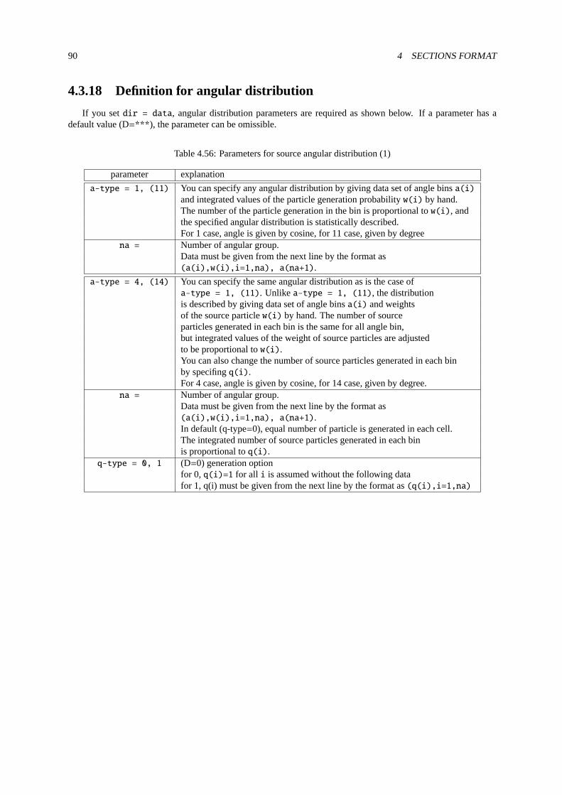
90 4 SECTIONS FORMAT
4.3.18 Definition for angular distribution
If you setdir = data, angular distribution parameters are required as shown below. If a parameter has adefault value (D=***), the parameter can be omissible.
Table 4.56:Parameters for source angular distribution (1)
parameter explanation
a-type = 1, (11) You can specify any angular distribution by giving data set of angle binsa(i)
and integrated values of the particle generation probabilityw(i) by hand.The number of the particle generation in the bin is proportional tow(i), andthe specified angular distribution is statistically described.For 1 case, angle is given by cosine, for 11 case, given by degree
na = Number of angular group.Data must be given from the next line by the format as(a(i),w(i),i=1,na), a(na+1).
a-type = 4, (14) You can specify the same angular distribution as is the case ofa-type = 1, (11). Unlike a-type = 1, (11), the distributionis described by giving data set of angle binsa(i) and weightsof the source particlew(i) by hand. The number of sourceparticles generated in each bin is the same for all angle bin,but integrated values of the weight of source particles are adjustedto be proportional tow(i).You can also change the number of source particles generated in each binby specifingq(i).For 4 case, angle is given by cosine, for 14 case, given by degree.
na = Number of angular group.Data must be given from the next line by the format as(a(i),w(i),i=1,na), a(na+1).In default (q-type=0), equal number of particle is generated in each cell.The integrated number of source particles generated in each binis proportional toq(i).
q-type = 0, 1 (D=0) generation optionfor 0, q(i)=1 for all i is assumed without the following datafor 1, q(i) must be given from the next line by the format as(q(i),i=1,na)

4.3 [ Source ] section 91
Table 4.57:Parameters for source angular distribution (2)
parameter explanation
a-type = 5, (15) Angular distributiondφ/dΩ(i) is given by g(x).For 5 case, angle is given by cosine, for 15 case, given by degree.
g(x) = Any analytical function of x, Fortran style.x denotes angle. One can use intrinsic functions and constants C.e.g.g(x) = exp(-c1*x**2)
nn = Number of angular group.ag1 = minimum cut off for angular distributionag2 = maximum cut off for angular distribution
a-type = 6, (16) You can specify the same angular distribution as is the case ofa-type = 5, (16). Unlike a-type = 5, (16), the number of sourceparticle generated in each bin is the same for all angle bin, butintegrated values of the weight of source particles are adjusted to beproportional tog(x).You can also change the number of source particles generated in each binby specifingq(i).for 6 case, angle is given by cosine, for 16 case, given by degree
g(x) = any analytical function of x, Fortran styleone can use intrinsic functions and constants C.
nn = Number of angular group.In default (q-type=0), equal number of particle is generated in each cell.The integrated number of source particles generated in each binis proportional toq(i).
ag1 = minimum cut off for angular distributionag2 = maximum cut off for angular distribution
q-type = 0, 1 (D=0) generation optionfor 0, q(i)=1 for all i is assumed without the following datafor 1, q(i) must be given from the next line by the format as(q(i),i=1,nn)
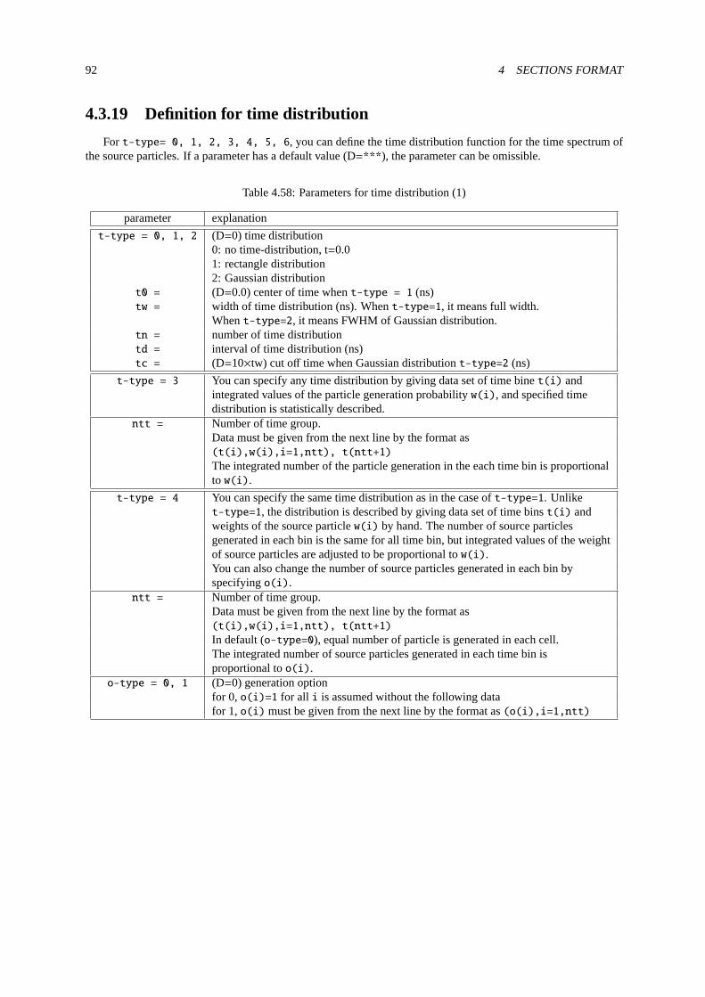
92 4 SECTIONS FORMAT
4.3.19 Definition for time distribution
Fort-type= 0, 1, 2, 3, 4, 5, 6, you can define the time distribution function for the time spectrum ofthe source particles. If a parameter has a default value (D=***), the parameter can be omissible.
Table 4.58:Parameters for time distribution (1)
parameter explanation
t-type = 0, 1, 2 (D=0) time distribution0: no time-distribution, t=0.01: rectangle distribution2: Gaussian distribution
t0 = (D=0.0) center of time whent-type = 1 (ns)tw = width of time distribution (ns). Whent-type=1, it means full width.
Whent-type=2, it means FWHM of Gaussian distribution.tn = number of time distributiontd = interval of time distribution (ns)tc = (D=10×tw) cut off time when Gaussian distributiont-type=2 (ns)
t-type = 3 You can specify any time distribution by giving data set of time binet(i) andintegrated values of the particle generation probabilityw(i), and specified timedistribution is statistically described.
ntt = Number of time group.Data must be given from the next line by the format as(t(i),w(i),i=1,ntt), t(ntt+1)
The integrated number of the particle generation in the each time bin is proportionalto w(i).
t-type = 4 You can specify the same time distribution as in the case oft-type=1. Unliket-type=1, the distribution is described by giving data set of time binst(i) andweights of the source particlew(i) by hand. The number of source particlesgenerated in each bin is the same for all time bin, but integrated values of the weightof source particles are adjusted to be proportional tow(i).You can also change the number of source particles generated in each bin byspecifyingo(i).
ntt = Number of time group.Data must be given from the next line by the format as(t(i),w(i),i=1,ntt), t(ntt+1)
In default (o-type=0), equal number of particle is generated in each cell.The integrated number of source particles generated in each time bin isproportional too(i).
o-type = 0, 1 (D=0) generation optionfor 0, o(i)=1 for all i is assumed without the following datafor 1, o(i)must be given from the next line by the format as(o(i),i=1,ntt)

4.3 [ Source ] section 93
Table 4.59:Parameters for time distribution (2)
parameter explanation
t-type = 5 Differential spectrum (dφ/dt) is given byh(t).h(x) Any analytical function of x(ns), Fortran style.
One can use intrinsic function and constantsC.ll Number of time group
If it is given by positive number, linear interpolation is assumed in a bin.If negative, logarithmic interpolation is assumed in a bin.Integrated number of source particles generated in each cell is proportional to h(x).
tg1 Minimum cut off for time distribution (ns)tg2 Maximum cut off for time distribution (ns)
t-type = 6 You can specify the same time distribution as in the case oft-type=5. Unlike t-type=5,the number of source particle generated in each bin is the same for all time bin, butintegrated values of the weight of source particles are adjusted to be proportional toh(x).You can also change the number of particles generated in each bin by specifyingo(x).
h(x) Any analytical function of x(ns), Fortran style.One can use intrinsic function and constantsC.
ll Number of time groupIf it is given by positive number, linear interpolation is assumed in a bin.If negative, logarithmic interpolation is assumed in a bin.In default (o-type=0), equal number of particle is generated in eachcell. The integrated number of source particles generated in each timebin is proportional too(i).
tg1 Minimum cut off for time distribution (ns)tg2 Maximum cut off for time distribution (ns)
o-type = 0, 1 (D=0) generation optionfor 0, o(i)=1 for all i is assumed without the following datafor 1, o(i)must be given from the next line by the format as(o(i),i=1,ntt)
When you sett-type=100, you can use an original distribution by defining its function in subroutine tdis01of sors.f, which a source file of PHITS.
Table 4.60:Parameters for time distribution (3)
parameter explanation
t-type = 100 User define time distribution. User can write any type of time distributionin the source program of sors.f
tg1 Minimum cut off for time distribution (ns)tg2 Maximum cut off for time distribution (ns)

94 4 SECTIONS FORMAT
4.3.20 Example of multi-source
We introduce an example of multi-source, which includes energy distribution and angular distribution describedby analytic functions. The list of third multi-source is shown below.
Example 4: Example of multi-source
1: [ S o u r c e ]
2: totfact = 3
3: <source> = 9.72
4: s-type = 1
5: proj = proton
6: z0 = 2
7: z1 = 29
8: r0 = 5
9: r1 = 4
10: dir = 0.0
11: e-type = 6
12: eg1 = 1.e-6
13: eg2 = 1.e-3
14: nm = -200
15: set: c10[1.e-4]
16: f(x) = x**(1.5)*exp(-x/c10)
17: <source> = 1
18: s-type = 1
19: proj = photon
20: z0 = 1
21: z1 = 2
22: r0 = 5
23: dir = -1
24: e-type = 5
25: eg1 = 1.e-3
26: eg2 = 5.e-1
27: nm = 200
28: set: c10[1.e-1]
29: set: c20[1.e-1/2.35482]
30: f(x) = exp(-(x-c10)**2/2/c20**2)
31: <source> = 1
32: s-type = 1
33: proj = neutron
34: z0 = 29
35: z1 = 30
36: r0 = 5
37: e-type = 6
38: eg1 = 1.e-2
39: eg2 = 1.e+3
40: nm = -200
41: set: c10[92.469]
42: set: c20[5.644e+10]
43: f(x) = c10/c20*exp(-sqrt(x*(x+1876))/c10)*(x+938)/sqrt(x*(x+1876))
44: dir = data
45: a-type = 5
46: ag1 = 0
47: ag2 = 1
48: nn = 200
49: g(x) = exp(-(x-1)**2/0.3**2)

4.3 [ Source ] section 95
In this example, there are three source subsections started from<source>. In the first source subsection, wedefine a cylinder source from z=2cm to z=29cm with 5cm radius, and we setr1=4. This r1=4 means that theregion inside the cylinder with radius 4cm is not included. In the next source, it is also a cylinder source fromz=1cm to z=2cm with 5cm radius withoutr1. This is a normal thin cylinder. The last one is also a thin cylinderfrom z=29cm to z=30cm with 5cm radius. The numbers defined after each<source> denote the relative weightof the multi-source. In this example, the relative weight is determined by the relative volume ratio of each source.This means that the source particles are generated uniformly in each source volume. The coordinate distributionof the generated source particles is shown in Fig.4.6using [t-product] tally with output=source, and icntl=6.
0 10 20 30
−6
−4
−2
0
2
4
6
z [cm]
x [c
m]
10−3
Num
ber
[1/c
m3 /s
ourc
e]
−6 −4 −2 0 2 4 6
−6
−4
−2
0
2
4
6
x [cm]
y [c
m]
z=1.5cm
10−3
Num
ber
[1/c
m3 /s
ourc
e]
−6 −4 −2 0 2 4 6
−6
−4
−2
0
2
4
6
x [cm]
y [c
m]
z=15cm
10−3
Num
ber
[1/c
m3 /s
ourc
e]
Figure 4.6:Multi-source, coordinate distribution
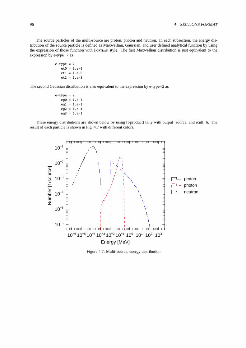
96 4 SECTIONS FORMAT
The source particles of the multi-source are proton, photon and neutron. In each subsection, the energy dis-tribution of the source particle is defined as Maxwellian, Gaussian, and user defined analytical function by usingthe expression of those function with Fortran style. The first Maxwellian distribution is just equivalent to theexpression by e-type=7 as
e-type = 7
et0 = 1.e-4
et1 = 1.e-6
et2 = 1.e-3
The second Gaussian distribution is also equivalent to the expression by e-type=2 as
e-type = 2
eg0 = 1.e-1
eg1 = 1.e-1
eg2 = 1.e-4
eg3 = 5.e-1
These energy distributions are shown below by using [t-product] tally with output=source, and icntl=6. Theresult of each particle is shown in Fig.4.7with different colors.
10−6 10−5 10−4 10−3 10−2 10−1 100 101 102 103
10−6
10−5
10−4
10−3
10−2
10−1
Energy [MeV]
Num
ber
[1/s
ourc
e]
proton
photon
neutron
Figure 4.7:Multi-source, energy distribution

4.3 [ Source ] section 97
The first source has an angular distribution defined by dir=0, which means 90 degrees direction with respect toz-axis, the second one has dir=-1, 180 degrees direction, and the third one has an angular distribution defined bya-type description in which we used an analytic function for an angular distribution. The angular distribution ofthe third one is shown in Fig.4.8by using [t-cross] tally.
0.0 0.2 0.4 0.6 0.8 1.00.0000
0.0005
0.0010
0.0015
cos(θ)
Ang
ular
dis
trib
utio
n
Figure 4.8:Multi-source, angular distribution

98 4 SECTIONS FORMAT
4.3.21 Duct source option
For the simulation of neutrons through the long beam-line from the moderator of spallation neutron source orthe reactor to the detector room, we have prepared the following duct source options to reduce the variance of thecalculations. The beam current transported through the beam-line decreases proportional to the inverse square ofthe distance from the moderator. This means that the current crossing the wall of the beam-line, which is called as”wall current”, at 100 m point is six order of magnitude smaller than that at 1 m point from the source if we assumeisotropic distribution of the source direction. To reduce this variance, we have introduced a special options of thesource function in which the wall current of the simulation particles is equalized at any point of the beam-line bychanging the importance weight of the particles to simulate a real situation of the current inside the beam-line.
We set the duct source options fors-type = 1, 2, circle and rectangle source, bydom = -10. The parame-ters for the duct source options are summarized in Table4.61.
Table 4.61:Parameters for duct source options
parameter explanation
dom = -10 specify the duct sourcedl0 = starting z position of the beam-line from z0[cm].dl1 = starting z position of the duct source from z0[cm].dl2 = ending z position of the duct source from z0[cm].dpf = portion of pass through particles at dl2drd = radius of circle beam line for s-type= 1[cm].dxw = x size of rectangle beam line for s-type= 2[cm].dyw = y size of rectangle beam line for s-type= 2[cm].
We assume circle or rectangle beam-line fors-type = 1 or 2, respectively.z1 = z0 anddir = 1 are alsoassumed, the latter means the direction of the beam-line. If you want to change the direction of the beam-line,you should use the transformationtrcl = number of transformation. The source particles are generated withinthe circle or rectangle region atz0 defined byr0 or x0, x1, y0, y1, for s-type = 1 or 2, respectively. Thedirection of the particle is determined by the wall position where it reaches withindl1 anddl2 so as to equalizethe wall current at any point within this region changing the importance of the particle. Overall normalizationfactor is defined as a number of the source particles which pass the entrance of beam-line atdl0 originated withinthe same region at the source positionz0 as that atdl0. We normally set the number to be unit for one history ifall duct wall position fromdl0 to dl2 can see the source region atz0. If the source region atz0 is larger than thearea of the beam-line atdl0, the source particle from the outer region atz0 is not counted as the normalizationnumber atdl0. This means that the extra region atz0 increases the current in the beam-line without changingthe normalization factor. In the above argument, we assume isotropic angular distribution of the source particleswithin the small solid angle which covers the whole beam-lin.
dl0 dl1 dl2z0
dxw
dyw
False
True
Figure 4.9: Schematic image of the duct source.
We show some example of the duct source option in the following. In the first example, we use the rectanglesource and beam-line, the same size of the source and beam-line dimensions. Here we show the input for the ductsource option,

4.3 [ Source ] section 99
Example 5: duct source option, example (1)
1 [ S o u r c e ]
2:
3: set: c1[200] $dl0
4: set: c2[500] $dl1
5: set: c3[5000] $dl2
6: set: c4[5.0] $x*2 at z0
7: set: c5[5.0] $y*2 at z0
8: set: c10[5.0] $dxw
9: set: c20[5.0] $dyw
10: set: c30[0.001] $dpf
11:
12: s-type = 2
13: proj = neutron
14: e0 = 20.0
15: x0 = -c4/2
16: x1 = c4/2
17: y0 = -c5/2
18: y1 = c5/2
19: z0 = 0.0
20: z1 = 0.0
21: dir = 1.0
22: phi = 0.0
23:
24: dom = -10
25: dl0 = c1
26: dl1 = c2
27: dl2 = c3
28: dxw = c10
29: dyw = c20
30: dpf = c30
In the first part of above source section, we define some constants which are necessary for the duct source option,dl0, dl1, dl2, size of source,dxw, dyw, dpf. In the second part, we define the position and xy region of thesource, direction of the beam-line and the energy of source particle. In the third part, we define the duct sourceoptions. We calculated particle transport in the beam-line from 5 m up to 50 m by this duct source and the current,wall current by using the cross tally. The results are shown in Fig.4.10compared with an ideal case in which thecurrent and the wall current are proportional to 1/L2 and 1/L3, respectively. The cross marker in the figure indicatesthe position ofdl0 and show that the current at this point is unit. The results of the duct source option agree verywell with the analytical results.
0 1000 2000 3000 4000 5000
10−6
10−5
10−4
10−3
10−2
10−1
100
101
z [cm]
Cur
rent
[n/s
ourc
e]
1 / L2
1 / L3
Current, PHITS
Wall Current, PHITS
Figure 4.10:Duct source option, example 1
In the next example, we changed only the size of the source from the previous example.

100 4 SECTIONS FORMAT
Example 6: duct source option, example (2)
1 [ S o u r c e ]
2:
3: set: c1[200] $dl0
4: set: c2[500] $dl1
5: set: c3[5000] $dl2
6: set: c4[10.0] $x*2 at z0
7: set: c5[10.0] $y*2 at z0
8: set: c10[5.0] $dxw
9: set: c20[5.0] $dyw
10: set: c30[0.001] $dpf
11:
12: s-type = 2
13: proj = neutron
14: e0 = 20.0
15: x0 = -c4/2
16: x1 = c4/2
17: y0 = -c5/2
18: y1 = c5/2
19: z0 = 0.0
20: z1 = 0.0
21: dir = 1.0
22: phi = 0.0
23:
24: dom = -10
25: dl0 = c1
26: dl1 = c2
27: dl2 = c3
28: dxw = c10
29: dyw = c20
30: dpf = c30
Figure4.11shows how the extra region of the source increases the current and the wall current. By this function,you can automatically treat the margin area of the moderator to the size of the cross-section of beam-line.
0 1000 2000 3000 4000 5000
10−6
10−5
10−4
10−3
10−2
10−1
100
101
z [cm]
Cur
rent
[n/s
ourc
e]
1 / L2
1 / L3
Current, PHITS
Wall Current, PHITS
Figure 4.11:Duct source option, example 2

4.4 [ Material ] section 101
4.4 [ Material ] section
4.4.1 Formats
Materials, which are used to define 3-dimensional geometry, are defined in this section. The defined materialsare refered to some sections such as[cell] section.
The[material] section is defined by material number, elements (or nuclides), and their composition ratios.Following a material number, element symbols and their ratios should be alternately written to define a compoundor mixture. The format is as follows:
[ M a t e r i a l ]
MAT[n] element ratio element ratio ... ...
Two formats to specify material numbers can be used as follows:MAT[n] andMn, wheren is a material number.Use any number from 1 to 99999. Note that a blank space cannot be set betweenMAT and[ in the formatMAT[n].
The following comment marks can be used:#, %, !, $. Although version 2.88 or before,c can be also usedas comment marks, after version 2.89, it is not permitted in the default setting. When you usec as comment marksin this section, seticommat=1 in [parameters] section. Note that the[parameters] section withicommat=1should be written above (before) the[material] section includingc. File including and variable definition canbe used in this section.
4.4.2 Element (nuclide) definition
Theelement in the above format can be specified using element symbols. To define nuclide (isotope), add itsmass number to the symbol as follows:208Pb, Pb-208, or 82208. For instance, hydrogen is defined as1H,H-1, or 1001. The natural abundance of isotopes can be defined using only an element symbol or a no-massstyle as, e.g., Pb, 82000. Note that the natural isotope ratio format cannot be used for an isotope not included inthe nuclear data library JENDL-4.0.
To use nuclear data libraries other than JENDL-4.0, copy all addresses of the new library and then paste it atthe end of the address filefile(7) (D=xsdir). When setting the new library of low-energy neutrons (below20MeV) other than JENDL-4.0, specify the “library id” in each material number byNLIB parameter, which isshown in Table4.62. The “library id” consists of the library number (double-digit) and data class (character a-z).For example,50c for the low-energy neutron data library of JENDL-4.0. The libraries of photons, electrons, andprotons can be also specified byPLIB, ELIB, HLIB, respectively. The library id can be specified by nuclideinstead of by material number following the element definition and a period as, e.g.,208Pb.50c, Pb-208.50c,
or 82208.50c. In PHITS, only one type of the library should be used for each incident particle, and the id shouldbe specified by theNLIB, PLIB, ELIB, HLIB parameters. Only for neutrons, the second library can be used;in this case, after specifying the library id byNLIB, define the nuclide by the expression of208Pb.50c. If thelibrary id is not specified by the user, PHITS searches the address filefile(7) (D = xsdir) from the top linefor the library number id corresponding to the nuclide and uses the corresponding data library. Information on thedata library used in a PHITS calculation is written in the summary output filefile(6) (D=phits.out) whenkmout=1 is set in the[parameters] section.
When using EGS5, restrict the number of elements (not nuclides) in one material number to 20.
4.4.3 Composition ratio definition
The composition ratios of the defined elements are given inratio in the above format. Two ways are availablefor the ratio definition: if ratio takes a positive value, it means atomic ratio; for negative value, it does mass ratio.For instance, water (H2O) can be defined as follows:
MAT[1] H 2 O 1
or

102 4 SECTIONS FORMAT
MAT[1] H -2/18 O -16/18
In the latter case, the mass ratios of hydrogen and oxygen are given as about 2/18 and 16/18, respectively, becausethe molecular mass of the water is about 18.
The material densities used in transport calculations are given in the[cell] section. Note that material den-sities must be defined in the[material] section instead of composition ratios when usingletmat parameterin [t-deposit], [t-deposit2], [t-let], [t-sed] sections. In this case, if it takes a positive value, theparticle density is[1024 atoms/cm3], and for negative value, it is given as a mass density[g/cm3].
4.4.4 Material parameters
For regions in which nuclear data are used, the material parameters for each material can be set using the formatkeyword=value. The parameters can be set anywhere in the material subsection. The full set of material parametersis listed in Table4.62.
Table 4.62:Material parameters
parameter value explanation
GAS D = 0 Density effect correction to electron stopping power= 0 Appropriate for materials in the condensed (solid or liquid) state used= 1 Appropriate for material in the gaseous state
ESTEP = n Make sub step numbern for electron transport:ignored whenn is smaller than the built-in default value
NLIB = id Change default neutron library numberidPLIB = id Change default photon library numberidELIB = id Change default electron library numberidHLIB = id Change default proton library numberidCOND Conductor settings
< 0 Non-conductor= 0 (default) Non-conductor if there exists at least 1 non-conductor; otherwise, conductor.> 0 Conductor if there exists at least 1 conductor.
4.4.5 S(α, β) settings
In the transport of low-energy neutrons, theS(α, β) library may be required. This library can be set as follows:
MTn materialID
wheren is the material number andmaterialID is the ID number, such aslwtr.20t, written in “xsdir”. See\XS\tsl\tsl-table for detailed information for these data.
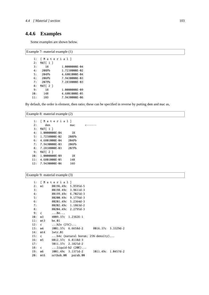
4.4 [ Material ] section 103
4.4.6 Examples
Some examples are shown below.
Example 7: material example (1)
1: [ M a t e r i a l ]
2: MAT[ 1 ]
3: 1H 1.0000000E-04
4: 208Pb 1.7238000E-02
5: 204Pb 4.6801000E-04
6: 206Pb 7.9430000E-03
7: 207Pb 7.2838000E-03
8: MAT[ 2 ]
9: 1H 1.0000000E-09
10: 14N 4.6801000E-05
11: 16O 7.9430000E-06
By default, the order is element, then ratio; these can be specified in reverse by puttingden andnuc as,
Example 8: material example (2)
1: [ M a t e r i a l ]
2: den nuc <------
3: MAT[ 1 ]
4: 1.0000000E-04 1H
5: 1.7238000E-02 208Pb
6: 4.6801000E-04 204Pb
7: 7.9430000E-03 206Pb
8: 7.2838000E-03 207Pb
9: MAT[ 2 ]
10: 1.0000000E-09 1H
11: 4.6801000E-05 14N
12: 7.9430000E-06 16O
Example 9: material example (3)
1: [ M a t e r i a l ]
2: m1 80196.49c 5.9595d-5
3: 80198.49c 3.9611d-3
4: 80199.49c 6.7025d-3
5: 80200.49c 9.1776d-3
6: 80201.49c 5.2364d-3
7: 80202.49c 1.1863d-2
8: 80204.49c 2.2795d-3
9: c ...Be...
10: m3 4009.37c 1.2362E-1
11: mt3 be.01
12: c ...h2o (25C)...
13: m4 1001.37c 6.6658d-2 8016.37c 3.3329d-2
14: mt4 lwtr.01
15: c ...b4c (natural boron; 25%-density)...
16: m5 6012.37c 6.8118d-3
17: 5011.37c 2.1825d-2
18: c ...liquid-h2 (20K)...
19: m6 1001.49c 3.1371d-2 1011.49c 1.0457d-2
20: mt6 orthoh.00 parah.00

104 4 SECTIONS FORMAT
4.5 [ Surface ] section
4.5.1 Formats
In this section, surfaces can be set to define cells in the[cell] section. You can set several surfaces such asplanes, sphere surfaces, cylindrical surfaces, and so on by giving parameters in equations of the shapes. OnlyC
and$ can be used as a comment mark. File including and variable definition can be used in this section. If youwant to use continuation lines, it is enough to put more than 4 blanks at the line head instead of the line sequentialmark at the end of line.
The[surface] section is defined in order by the data: surface number, coordinate transform number, surfacesymbol, and surface definition. These are explained in Table4.63. The format is shown below.
[ S u r f a c e ]
surface number transform number surface symbol surface definition
As a surface symbol, you can specify surfaces expressed by equations in Table4.64or macro body in Table4.64. You can use mathematical expressions and user defined variables in the surface definition. You can also usereflective and white boundary conditions by writing “*” and “+”, respectively, before the surface number. Forexample, “*10” indicates that surface 10 is a reflective boundary. The reflective boundary condition is useful todevelop an infinite repeated structure.
Table 4.63:Surface Definition Format
item explanation
surface number You can use any number from 1 to 999999.transform number Specify the numbern of TRn defined in[transform] section.
Not specify it when you don’t use coordinate transform.surface symbol Specify a surface symbol in Tables4.64and4.65.surface definition Speciry parameters of 1∼ 15 inputs, which depend on the
surface symbol.

4.5 [ Surface ] section 105
Table 4.64:Surfaces Expressed by Equations
Surface Symbol Type Explanation Equation Parameters
P plane multi-purpose Ax+ By+Cz− D = 0 A, B, C, DPX vertical with X-axis x− D = 0 DPY vertical with Y-axis y− D = 0 DPZ vertical with Z-axis z− D = 0 DP plane defined by x1, y1, z1, x2, y2, z2,
3 coordinates x3, y3, z3
SO sphere origin is center x2 + y2 + z2 − R2 = 0 RS multi-purpose (x− x0)2 + (y− y0)2 + (z− z0)2 − R2 = 0 x0, y0, z0, R
SX center on X-axis (x− x0)2 + y2 + z2 − R2 = 0 x0, RSY center on Y-axis x2 + (y− y0)2 + z2 − R2 = 0 y0, RSZ center on Z-axis x2 + y2 + (z− z0)2 − R2 = 0 z0, RC/X cylinder parallel with X-axis (y− y0)2 + (z− z0)2 − R2 = 0 y0, z0, RC/Y parallel with Y-axis (x− x0)2 + (z− z0)2 − R2 = 0 x0, z0, RC/Z parallel with Z-axis (x− x0)2 + (y− y0)2 − R2 = 0 x0, y0, RCX on X-axis y2 + z2 − R2 = 0 RCY on Y-axis x2 + z2 − R2 = 0 RCZ on Z-axis x2 + y2 − R2 = 0 R
K/X cone parallel with X-axis√
(y− y0)2 + (z− z0)2 ∓ |t| (x− x0) = 0 x0, y0, z0, |t|2 , kK/Y parallel with Y-axis
√(x− x0)2 + (z− z0)2 ∓ |t| (y− y0) = 0 x0, y0, z0, |t|2 , k
K/Z parallel with Z-axis√
(x− x0)2 + (y− y0)2 ∓ |t| (z− z0) = 0 x0, y0, z0, |t|2 , kKX on X-axis
√y2 + z2 ∓ |t| (x− x0) = 0 x0, |t|2 , k
KY on Y-axis√
x2 + z2 ∓ |t| (y− y0) = 0 y0, |t|2 , kKZ on Z-axis
√x2 + y2 ∓ |t| (z− z0) = 0 z0, |t|2 , k
k is ±1 or unspecifiedSQ ellipse, parallel with A(x− x0)2 + B(y− y0)2 +C(z− z0)2 A, B, C, D, E,
hyperboloid, X-, Y-, +2D(x− x0) + 2E(y− y0) + 2F(z− z0) F, G, x0, y0, z0
paraboloid or Z- axis +G = 0GQ cylinder, non parallel with Ax2 + By2 +Cz2 + Dxy+ Eyz+ A, B, C, D, E,
cone, X-, Y- and Fzx+Gx+ Hy+ Jz+ K = 0 F, G, H, J, Kellipse, Z-axis
hyperboloid,paraboloid
TX ellipse torus parallel with (x− x0)2/B2+ x0, y0, z0, A, B, Ctorus X-, Y-, or (
√(y− y0)2 + (z− z0)2 − A)2/C2 − 1 = 0
TY Z-axis (y− y0)2/B2+ x0, y0, z0, A, B, C(√
(x− x0)2 + (z− z0)2 − A)2/C2 − 1 = 0TZ (z− z0)2/B2+ x0, y0, z0, A, B, C
(√
(x− x0)2 + (y− y0)2 − A)2/C2 − 1 = 0
When you use surfaces, which are defined in[surface] section, in[cell] section, inside of the shape shouldbe basically specified as “negative sense”, and its outside should be done as “positive sense”. Note that in the caseof unclosed shapes such as planes, you have to distinguish which side of the plane is “positive” or “negative” bycalculating a value off (x, y, z) at a point (x0, y0, z0), where f (x, y, z) is an equation of the unclosed shape. Iff (x0, y0, z0) > 0, the side including the point is “positive”, and iff (x0, y0, z0) < 0, the side is “negative”. Forexample, in the case ofPY with D = 5, the side including the origin (0,0,0) is “negative” becausef (0,0,0) =−5 < 0.
You can define a plane by settingx, y, z-coordinates of 3 points with the symbolP. In this case, a regionincluding the origin is of negative sense.
The cone defined byx0, y0, or z0 has two sheets as the center being the coordinate of the top along the directionof each axis. If you set to be 1 fork, the upper sheet is used, and the lower sheet is used in the case of−1. Whenk is not specified, both sheets are used. It should be noted that you have to use a plane passing the top when youdefine a region in[cell] section using only one side of the cones; you have to use three surface, a plane passingthe top, a side sheet of the cone, and an underside of the cone, in the definition.

106 4 SECTIONS FORMAT
When you useTX,TY,TZ to define ellipse torus or torus, you cannot transform their coordinates by setting[transform] section.
Table 4.65:Macro Body
Symbol Type Parameters Explanation
x0, y0, z0, Base point coordinateBOX Optional BOX Ax, Ay, Az, Vector from base point to first surface.
(all angles are 90) Bx, By, Bz, Vector from base point to second surface.Cx, Cy, Cz Vector from base point to third surface.
RPP Rectangular solid xmin, xmax, Minimum and Maximum ofx.(Each surface is vertical ymin, ymax, Minimum and Maximum ofy.
with x, y, z axes) zmin, zmax Minimum and Maximum ofz.SPH Sphere x0, y0, z0, Center coordinate.
(the same with general sphere S) R Radius.x0, y0, z0, Center coordinate of bottom face.
RCC Cylinder Hx, Hy, Hz, Height vector from center of bottom face to that of top face.R Radius.
x0, y0, z0, Base point coordinate.RHP Optional hexagonal prism Hx, Hy, Hz, Height vector from base point.or Prism Ax, Ay, Az, Vector from base point to first surface.
HEX Bx, By, Bz, Vector from base point to second surface.Cx, Cy, Cz Vector from base point to third surface.
REC Right elliptical cylinder x0 y0 z0, Center coordinate of bottom face.Hx, Hy, Hz, Height vector from center of bottom face (H).Ax, Ay, Az, Major axis vector of ellipse orthogonal toH (A).Bx, By, Bz Minor axis vector of ellipse orthogonal toH andA (B).
TRC Truncated right-angle cone x0, y0, z0, Center coordinate of bottom face of cone.Hx, Hy, Hz, Height vector from center of bottom.
R1, Radius of bottom face.R2 Radius of top face.
ELL Ellipsoid of revolution If R> 0,(Spheroid) x1, y1, z1, Coordinate of first focus.
x2, y2, z2, Coordinate of second focus.R Radius of major axis.
If R< 0, In this case, ellipsoid is made by rotating on major axis.You can set to be major axis< minor axis.
x0, y0, z0, Center coordinate of ellipsoid.Ax, Ay, Az, Major axis vector.
R Radius of minor axis.WED Wedge x0, y0, z0, Coordinate of top.
Ax, Ay, Az, Vector to first side of triangle (A).Bx, By, Bz, Vector to socond side of triangle (B).Hx, Hy, Hz Height vector (H).
You cannot setR2 to 0 in definition ofTRC. If you want to define a usual cone, i.e. not truncated cone, usingTRC, you should setR2 to a small value.
The bottom of the wedge defined byWED must be a right triangle. When you make a arbitrary triangle, youhave to combine right triangles various sizes.

4.5 [ Surface ] section 107
4.5.2 Examples
This section shows examples of the surface definition listed in Table4.64and4.65.
Example 10: Example of Plane (1)
1: [surface]
2: 1 PY 5
z
xy
y=5
5
Figure 4.12: The plane ofy = 5 defined inExample10.
PX,PY,PZ define planes perpendicular tox, y, z axes, respectively.In this example, a plane of surface number 1, which isy = 5 andperpendicular toy axis, is defined by setting the symbol to bePY andthe parameter to beD = 5. The surface number 1 corresponds to aplane denoted by dashed line in Fig.4.12.
Example 11: Example of Plane (2)
1: [surface]
2: 1 P 2 2 1 10
3: 2 P 5 0 0 0 5 0 0 0 10
z
x
y
2x+2y+z-10=0
10
55
Figure 4.13: The plane defined in Exam-ple11.
You can define arbitrary planes by specifyingP as the symbol.In this case, there are two kinds of the description to define theplane. One is to give the four parametersA, B,C,D in an equationAx+ By+ Cz− D = 0, and the other is to setx, y, z-coordinates of3 points, (x1, y1, z1), (x2, y2, z2), (x3, y3, z3). You can use the formerkind when you know a normal vector (s, t,u) of the plane andx, y, z-coordinates of a point, (x0, y0, z0), on the plane. An equation of theplane satisfying these conditions is given as
s(x− x0) + t(y− y0) + u(z− z0) = 0. (6)
Because we have
sx+ ty+ uz− (sx0 + ty0 + uz0) = 0, (7)
we can define an arbitrary plane by settingA = s, B = t,C = u,D = sx0 + ty0 + uz0. The surface number 1shown in Example11 is defined as a plane having the normal vector (2,2,1) and passing the coordinate (5,0,0).This surface corresponds to a plane denoted by dashed line in Fig.4.13. In the latter kind, you specifyx, y, z-coordinates of 3 points. The surface number 2 in Example11 is defined as a plane passing the 3 coordinates(5,0,0), (0,5,0), (0,0,10). This surface is the same as that of the surface 1.

108 4 SECTIONS FORMAT
Example 12: Example of Sphere Surface
1: [surface]
2: 1 SO 5
3: 2 SZ 10 3
4: 3 S 10 10 0 3
z
x
y
10
10
10
Surface Number 1
Surface Number 2
Surface Number 3
Figure 4.14: The three sphere surfaces defined in Example12.
When you define sphere surfaces, you specifythe symbolsSO,SX,SY,SZ,S. You can useSOto define a sphere surface centered at the originwith specifying its radiusR as a parameter. Inthe 2nd line of Example12, a sphere surfacecentered at the origin with a radius of 5 cm isdefined as the surface number 1. The symbolsSX,SY,SZ can be used to define sphere surfacescentered onx, y, z axes, respectively. You haveto specify two parameters, a coordinate valueon the axis and a radius of the sphere. In the 3rdline of Example12, a sphere surface centered atthe coordinate (0,0,10), which is a point on thez axis, with a radius of 3 cm is defined as the surface number 2.When you define a sphere surface centered at an arbitrary coordinate (x0, y0, z0), you can use the symbolS. Inthis case, you have to specify four parameters, the coordinate valuesx0, y0, z0, and the radiusR. In the 4th line ofExample12, a sphere surface centered at the coordinate (10,10, 0) with a radius of 3 cm is defined as the surfacenumber 3. The three sphere surfaces defined in Example12are shown in Fig.4.14.
Example 13: Example of Cylinder Surface
1: [surface]
2: 1 CY 5
3: 2 C/Y 15 0 3
z
x
y
Surface Number 1
Surface Number 2
R=5
R=3
Figure 4.15: The two cylinder surfaces de-fined in Example13.
When you define a cylinder surface having a central axis ofx, y, zaxes, you specify the symbolCX,CY,CZ, respectively. In this case,you have to specify its radiusR as a parameter. In the 2nd line ofExample13, a cylinder surface having a central axis of they axis witha radius of 5cm is defined. This surface corresponds to the surfaceof the cylinder shown in the right-upper side of Fig.4.15. You canuse the symbolsC/X,C/Y,C/Z, when you define cylinder surfaceshaving a central axis parallel tox, y, zaxes, respectively. In this case,you have to specify two coordinate values and a radius of the cylinder.In the 3rd line of Example13, a cylinder surface having a central axisparallel to they axis is defined. The two coordinate valuesx0 =
15, z0 = 0 are specified as the 1st and 2nd parameters, respectively,and the radius is given as the 3rd parameter. This surface correspondsto the surface of the cylinder in the left-lower side of Fig.4.15.
If you define a cylinder surface having a central axis NOT parallel tox, y, z axes, you can use the symbolGQ.However, it is easier to useCX,CY,CZ,C/X,C/Y,C/Z with a coordinate transformation by[transform] sectionthan to useGQ.

4.5 [ Surface ] section 109
Example 14: Example of Cone Surface
1: [surface]
2: 1 KZ 0 1
3: 2 K/Z 0 20 0 1/3 1
You can define cone surfaces having a central axis ofx, y, zaxes by specifying the symbolsKX,KY,KZ, respectively.As parameters, you have to give a coordinate value, an angle parameter|t|2, and a sheet parameterk (omissible).
z
xy
Surface Number 1
45o
Surface Number 2
20
30o
Figure 4.16: The cone surface defined in Example14.
An example specifyingKZ is shown in the 2ndline of Example14, The first parameter is thez-coordinate of the vertex of the cone,z0 = 0, and thesecond one is|t|2 = 1. The equation ofKZ is√
x2 + y2 ∓ |t| (z− z0) = 0. (8)
After substituting each parameters, we obtain theequations shown below.√
x2 + y2 − z= 0, (z> 0) (9)√x2 + y2 + z= 0, (z< 0) (10)
In this case, a surface of the surface number 1 is defined as the cone surface having a central axis of thezaxis withthe vertex at (0,0,0). This surface corresponds to the cone shown in the left side of Fig.4.16. The cone in the regionof z> 0 is represented by Eq. (9), and that inz< 0 is by Eq. (10). The surfaces inz> 0 andz< 0 can be specifiedby k = 1 andk = −1, respectively. Note thatk is not specified in the 2nd line of the example. In this case, bothtwo surfaces are defined. The parameter|t|2 has a relation of|t|2 = tan2 θ, whereθ is the angle between the centralaxis and the generating line. In the case of the surface number 1, tanθ = 1, therefore,θ = 45. When you definecone surfaces having a central axis parallel tox, y, zaxes and a vertex of the coordinate (x0, y0, z0), you specify thesymbolsK/X,K/Y,K/Z. In the 3rd line of Example14, an example specifyingK/Z is shown. The coordinate of thevertex is (0,20,0). This cone has a central axis parallel to thez axis. The angleθ is = 30, because of|t|2 = 1/3,namely tanθ = 1/
√3. In this case, only one cone surface in the region ofz> 0 is defined by specifyingk = 1.
Example 15: Example of Ellipsoid Surface
1: [surface]
2: 1 SQ 1/9**2 1/6**2 1/3**2 0 0 0 -1 0 0 0
z
xy
a=9 b=6c=3
Figure 4.17: The ellipsoid surfacedefined in Example15.
When you define an ellipsoid surface as shown in Fig.4.17, you specify thesymbolSQ. An equation of ellipsoid surfaces is given as
x2
a2+
y2
b2+
z2
c2= 1 (11)
wherea,b, c are lengths of the semi-principal axes alongx, y, zaxes, respec-tively. Therefore, you can define an ellipsoid surface by specifying fromthe 1st to the 7th parameters ofSQ as A = 1/a2, B = 1/b2,C = 1/c2,D = E = F = 0, andG = −1. In Example15, an ellipsoid surface withthe lengths ofa = 9,b = 6, c = 3 cm is defined. If you want to define aspheroid surface, you have to specify so that the two lengths along the two axes other than the rotational axis havethe same value. For example, in the case that thex axis is the rotational axis, you have to setb = c, namelyB = C.The 8,9,10th parameters ofSQ correspond to the coordinate of the center (x0, y0, z0), respectively. In Example15,the center of the ellipsoid is the origin (0, 0,0). Note that if you setD,E, F to non-zero value, you define quadricsurfaces other than ellipsoid surfaces.

110 4 SECTIONS FORMAT
Example 16: Example of Hyperboloid Surface
1: [surface]
2: 1 SQ 1/6**2 1/3**2 -1/5**2 0 0 0 -1 0 0 0
3: 2 SQ -1/6**2 -1/3**2 1/5**2 0 0 0 -1 0 20 0
By specifying the symbolSQ, you can define hyperboloid surfaces as shown in the center and right side of Fig.4.18.The surface in the center is called hyperboloid of one sheet, and those in the right side are hyperboloid of two sheets.Equations of the hyperboloid of one and two sheets are given as, respectively,
z
xy
(0,20,0)x
ya=6
b=3
z=0
Figure 4.18: The hyperboloid surface defined in Example16.
x2
a2+
y2
b2− z2
c2= 1, (12)
− x2
a2− y2
b2+
z2
c2= 1. (13)
Here, the central axis is thez axis.If a = b, the shape is called a hy-perboloid of revolution. The surfacenumber 1 defined in the 2nd line ofExample16 corresponds to the hy-perboloid of one sheet shown in thecenter of Fig.4.18. In the 2nd line,from the 1st to the 7th parameters ofSQ are given asA = 1/62, B = 1/32,C = −1/52, D = E = F = 0, andG = −1. The central axis is thez axis. Thisaxis passes through the origin because from the 8th to the 10th parameters are set asx0 = 0, y0 = 0, z0 = 0. Theintersection line of this hyperboloid with a plane vertical to thez axis is an ellipse. The figure in the left side ofFig.4.18shows the intersection line of the surface number 1 with the planez = 0. This ellipse has the major andminor radii ofa = 6 cm andb = 3 cm, respectively. The surface defined in the 3rd line of Example16correspondsto the hyperboloid of two sheets shown in the right side of Fig.4.18. In this case, the signs ofa,b, c of the surfacenumber 1 are reversed, andD = E = F = 0 andG = −1 are specified to define the hyperboloid of two sheets.Note that the central axis passes through the coordinate (0,20,0) by setting (x0, y0, z0) = (0,20,0) as the 8,9,10thparameters. When a surface of a hyperboloid of two sheets is used to define a cell in[cell] section, a region ofthe coordinate (x0, y0, z0) is “negative sense”, and the other region is “positive sense”. Therefore, the inside of thetwo sheets shown in the right side of Fig.4.18should be specified as “positive”.
Example 17: Example of Paraboloid Surface
1: [surface]
2: 1 SQ 1 1/2**2 0 0 0 -1 0 0 0 0
When you define a paraboloid surface as shown in Fig.4.19, you specify the symbolSQ as described in Example17.
z
xy
yx
z z
z=x2
x=0y=0
z= y 2
41
Figure 4.19: The paraboloid surface defined in Example17.
An equation of aparaboloid surfacewith the central axisof the z axis isgiven as
z=x2
a2+
y2
b2. (14)
Therefore, you candefine such surfaceby specifyingA =1/a2, B = 1/b2,C = 0, D = E = 0, F = −1, andG = 0 as from the 1st to the 7th parameters ofSQ. In the example,the paraboloid witha = 1,b = 2 is defined. The intersection line of this paraboloid with a plane including thezaxis is a parabola. The intersection lines of the paraboloid withy = 0 andx = 0 are shown in the left and rightpanels of Fig.4.19, respectively. The coordinate of the vertex can be specified by 8,9,10th parameters. In this case,x0 = 0, y0 = 0, z0 = 0 are set.

4.5 [ Surface ] section 111
Example 18: Example ofGQ
1: [surface]
2: set: c1[30]
3: set: c2[cos(c1/180*pi)]
4: set: c3[sin(c1/180*pi)]
5: 1 GQ c2**2 1/2**2 c3**2 0 0 -2*c2*c3 -c3 0 -c2 0
z
xy
Figure 4.20: The paraboloid sur-face defined in Example18.
You can define arbitrary surfaces expressed by quadratic equations ofx, y, zby specifying the symbolGQ. Although there are the similar surfaces suchasCX,KX,SQ, which are also expressed by quadratic equations,GQ can rep-resent quadratic surfaces having a central axis NOT parallel tox, y, z axes.Note that it is easier to useCX,KX,SQ with a coordinate transformation by[transform] section than to useGQ. Example18 represents a paraboloidsurface obtained by rotating the surface of Example17 an angle of 30
around they axis. The result is shown in Fig.4.20. The parameters of thisexample were obtained by calculating the following equations. When a co-ordinate (x′, y′, z′) is defined by rotating a coordinate (x, y, z) an angle ofθaroundy axis, the relation between the two coordinates is given as, x′
y′
z′
= cosθ 0 sinθ
0 1 0− sinθ 0 cosθ
x
yz
. (15)
From this relation, we can obtain xyz
= cosθ 0 − sinθ
0 1 0sinθ 0 cosθ
x′
y′
z′
= x′ cosθ − z′ sinθ
y′
x′ sinθ + z′ cosθ
. (16)
After substitution of this result in Eq. (14), we obtain the following equation ofx′, y′, z′.
x′ sinθ + z′ cosθ =(x′ cosθ − z′ sinθ)2
a2+
y′2
b2,
x′ sinθ + z′ cosθ =x′2 cos2 θ + z′2 sin2 θ − 2x′z′ cosθ sinθ
a2+
y′2
b2,
x′ sinθ + z′ cosθ =cos2 θ
a2x′2 +
sin2 θ
a2z′2 − 2 cosθ sinθ
a2x′z′ +
y′2
b2,
0 =cos2 θ
a2x′2 +
1b2
y′2 +sin2 θ
a2z′2 − 2 cosθ sinθ
a2x′z′ − x′ sinθ − z′ cosθ (17)
After comparing this result with the equation ofGQ in Table4.64and specifying their parameters, we can define aparaboloid surface rotatedθ aroundy axis. In this example,θ = 30 is given as a constantc1. Constantsc2,c3 arealso defined as sinθ, cosθ, respectively.

112 4 SECTIONS FORMAT
Example 19: Example of Torus Surface
1: [surface]
2: 1 TZ 0 0 0 10 3 5
A torus surface as shown in the center of Fig.4.21 can be obtained by rotating an ellipse around a rotationalaxis outside the ellipse. In PHITS, you can define torus surfaces having the rotational axis of thex, y, z axes byspecifying the symbolsTX,TY,TZ, respectively. An equation of a torus surface with the rotational axis of thezaxisis given as, ( √
x2 + y2 − R)2
a2+
z2
b2= 1. (18)
In this case, the ellipse has the major and minor radii ofa andb, respectively, and a distance between the centerof the ellipse and the rotational axis is given byR. The torus surface in Example19 has the center of the originby setting all the 1st, 2nd, and 3rd parameters ofTZ to 0. The 4,5,6th parameters are given asA = R = 10cm,B = b = 3cm, andC = a = 5cm, respectively. The intersection line of the torus with the planez = 0 is shown inthe left panel of Fig.4.21. The distance between thez axis and the center of the ellipse is 10 cm, and the width ofthe ring is 5· 2 = 10 cm. The intersection line of the torus withy = 0 is shown in the right panel of Fig.4.21. Notethat only the region ofx > 0 is shown. The major and minor radii of the ellipse are 5 and 3 cm, respectively.
z
xy
x
y zy=0z=0
R=10
x
a=5 R=10
a=5
b=3
Figure 4.21: The torus surface defined in Example19.
Example 20: Example ofBOX
1: [surface]
2: 1 BOX 5 5 0 9 0 0 0 6 0 0 0 3
z
xy
P(x ,y ,z )
=(5,5,0)
0 0 0
A(A ,A ,A )
=(9,0,0)
B(B ,B ,B )
=(0,6,0)
C(C ,C ,C )
=(0,0,3)
x
x
x
y
y
y
z
z
z
Figure 4.22: The rectangular surface defined in Ex-ample20.
By specifying the symbolBOX, you can define surfaces ofan arbitrary rectangular solid. As parameters ofBOX, youhave to give a coordinate of the base pointP(x0, y0, z0),and each components of three vectorsA(Ax,Ay,Az),B(Bx, By, Bz), andC(Cx,Cy,Cz). Figure4.22shows the re-lation between the basepoint and the three vectors. In Ex-ample20, the coordinate of the basepoint is (5,5, 0), andthe three vectors are given asA = (9, 0,0), B = (0,6,0),and C = (0,0,3). When you useBOX, vectorsA, B,Cdon’t have to be parallel tox, y, z axes, however, the vec-tors should be vertical to each other.

4.5 [ Surface ] section 113
Example 21: Example ofRPP
1: [surface]
2: 1 RPP 5 14 5 11 0 3
z
x
yx =5
y =5y =11
x =14
z =3z =0min
min
max
max min
max
Figure 4.23: The rectangular surface definedin Example21.
When you define surfaces of a rectangular solid surrounded bythree sets of two planes parallel toxy, yz, zx planes, you can usethe symbolRPP. UnlikeBOX, an arbitrary rectangular solid havingsurfaces NOT parallel tox, y, z axes cannot be defined. You haveto determine six parameters ofRPP, the maximum and minimumvalues for thex, y, zcoordinates. In Example21, xmin = 5, xmax =
14,ymin = 5, ymax = 11, andzmin = 0, zmax = 3 are specified as thesix parameters. The result is the same rectangular solid as definedin Example20, and shown in Fig.4.23.
Example 22: Example ofSPH
1: [surface]
2: 1 SPH 5 5 5 5
z
x
yx =5
y =5z =50
0
0
R =5
Figure 4.24: The sphere surface defined inExample22.
You can define a sphere surface with a center of an arbitrary coor-dinate by the symbolSPH. The 1st, 2nd, 3rd parameters are com-ponents of the coordinate (x0, y0, z0), and the 4th parameter is aradius of the sphere. The sphere surface with the center of thecoordinate (5,5,5) and the radius of 5 cm is defined in Example22. There is no difference betweenSPH and the symbolS.
Example 23: Example ofRCC
1: [surface]
2: 1 RCC 5 5 0 0 0 10 5
z
x
y
R =5
P(x ,y ,z )=(5,5,0)0 0 0
H(H ,H ,H )=(0,0,10)x y z
Figure 4.25: The cylinder surface defined inExample23.
By specifying the symbolRCC, you can define an arbitrary cylin-der surface. Parameters ofRCC are components of the center ofthe bottomP(x0, y0, z0), those of a vector from the bottom to thetop H(Hx,Hy,Hz), and a radius of the cylinderR. The relation be-tween these parameters is shown in Fig.4.25. In Example23, thecoordinateP(5,5,0) is the center of the bottom circle, the vectoris H = (0,0,10), and the radius is 5 cm. Unlike the symbols suchasCX andC/X, it is useful to define a cylinder surface having acentral axis NOT parallel tox, y, z axes.

114 4 SECTIONS FORMAT
Example 24: Example ofRHP
1: [surface]
2: 1 RHP 0 0 0 0 0 10 5 0 0 2 -5 0 -2 -5 0
To define hexagonal prism surfaces as shown in the right panel of Fig.4.26, you can use the symbolRHP or HEX. Asparameters of the symbols, you have to specify each components of the center coordinate of the bottomP(x0, y0, z0),those of a vector from the bottom to the topH(Hx,Hy,Hz), and those of three vectorsA(Ax,Ay,Az), B(Bx, By, Bz),C(Cx,Cy,Cz). The three vectorsA, B,C are required to define the hexagon of the bottom and top surfaces. The leftpanel of Fig.4.26shows the relation between the pointP and the three vectors. Namely, lengths and directions ofperpendicular lines between the pointP and the continuous three sides of the hexagon determine the three vectors.In Example24, the origin is the center of the bottom, and the height along thez axis of the hexagonal prism is 10cm. The components of the origin (0,0,0) are specified as the 1st, 2nd, 3rd parameters ofRHP, and those of thevectorH(Hx,Hy,Hz) = (0,0,10) are given as the 4, 5, 6th parameters. From the 7th to 15th parameters are thex, y, z components ofA, B,C. The defined hexagon shown in the left panel of the figure is symmetric with respectto they axis.
z
x
y
P(x ,y ,z )=(0,0,0)0 0 0
H(H ,H ,H )=(0,0,10)x y z
x
y
z=0
A(A ,A ,A )=(5,0,0)x y z
B(B ,B ,B )
=(2,-5,0)
x y z
C(C ,C ,C )=(-2,-5,0)x y z
P
Figure 4.26: The hexagonal prism surface defined in Example24.
Example 25: Example ofREC
1: [surface]
2: 1 REC 0 0 0 0 0 10 5 0 0 0 2 0
z
xy
P(x ,y ,z )=(0,0,0)0 0 0
H(H ,H ,H )=(0,0,10)x y z
A(A ,A ,A )=(5,0,0)x y z
B(B ,B ,B )=(0,2,0)x y z
P
x
y
z=0
Figure 4.27: The elliptical cylinder surface defined in Example25.
When you define elliptical cylin-der surfaces as shown in theright panel of Fig.4.27, you spec-ify the symbol REC. Parame-ters of REC are each compo-nents of the center coordinateof the bottomP(x0, y0, z0), thoseof a vector from the bottom tothe topH(Hx,Hy,Hz), and thoseof two vectorsA(Ax,Ay,Az) andB(Bx, By, Bz). The relation be-tween the pointP and the twovectorsA andB is shown in theleft panel of Fig.4.27. You haveto define the major and minor axis vectorsA andB with an initial pointP, which is the center of the ellipse. Thesurfaces of the elliptical cylinder having the height along thezaxis of 10 cm are defined in Example25. The centerof the bottom is the origin. The 1st, 2nd, 3rd parameters ofREC are the components of the origin (0, 0,0), and the4, 5, 6th parameters are those of the vectorH(Hx,Hy,Hz) = (0,0,10). Thex, y, zcomponents ofA andB are givenas from the 7th to 12th parameters. The two vectorsA andB are used to form the ellipse shown in the left panelof the figure.

4.5 [ Surface ] section 115
Example 26: Example ofTRC
1: [surface]
2: 1 TRC 0 0 0 0 0 10 5 2
z
xy
P(x ,y ,z )=(0,0,0)0 0 0
H(H ,H ,H )=(0,0,10)x y z
R =5
R =2
1
2
Figure 4.28: The cut cone surface defined in Ex-ample26.
You can define surfaces of a truncated right-angle cone asshown in Fig.4.28by specifying the symbolTRC. As parame-ters ofTRC, you have to specify each components of the cen-ter coordinate of the bottomP(x0, y0, z0), those of a vectorfrom the bottom to the topH(Hx,Hy,Hz), and two radii ofthe bottom and top circles,R1 and R2. In Example26, thesurfaces of the truncated right-angle cone the height along thez axis of 10 cm are defined. The center of the bottom circleis the origin. The components of the origin (0,0,0) are spec-ified as the 1st, 2nd, 3rd parameters, and those of the vectorH(Hx,Hy,Hz) = (0,0,10) are given as the 4, 5, 6th parame-ters. The radius of the bottom isR1 = 5 cm, and that of thetop isR2 = 2 cm. TheR1 andR2 are specified as the 7 and 8thparameters, respectively.
You cannot setR2 to 0 in definition ofTRC. If you want to define a usual cone, i.e. not truncated cone, usingTRC, you should setR2 to a small value.
Example 27: Example ofELL (1)
1: [surface]
2: 1 ELL 3 3 0 -3 -3 0 9
P(x ,y ,z )=(3,3,0)1 1 1x
y
z=0
P
1
P(x ,y ,z )=(-3,-3,0)2 2 22
P1
2
2R=18
y
x
z
Figure 4.29: The spheroid surface defined in Example27.
By specifying the symbolELL, you candefine a surface of an ellipsoid of rev-olution (a spheroid). After defining anellipse by specifying coordinates of twofocal points or a coordinate of its cen-ter, an ellipsoid of revolution is definedby rotating the ellipse around its majoraxis. Note that the meaning of the first6 parameters ofELL depends on the signof the 7th parameterR. Example27 isan example ofR > 0. In this case, youhave to give the coordinates of the two focal points and a radius of the major axis. The coordinate of the first focusP1(x1, y1, z1) is given as the 1st, 2nd, 3rd parameters, and that of the second oneP2(x2, y2, z2) is as the 4,5,6thparameters. The 7th parameter is the radius of the major axisR. The surface of the ellipsoid of revolution definedin Example27 is shown in the right side of Fig.4.29. The first and second focal points areP1(x1, y1, z1) = (3,3,0)andP2(x2, y2, z2) = (−3,−3,0), respectively. The ellipse is on thexy plane as shown in the left panel of Fig.4.29.An angle between the major axis and thex axis is 45. The length of the major axis is 2R = 18 cm. The ellipsoidis defined by rotating this ellipse around the major axis.
Although you can also define an ellipsoid surface bySQ, it is easier to define an ellipsoid having an inclinedrotational axis byELL than bySQ. Note that you can define only surfaces of ellipsoids of revolution byELL.

116 4 SECTIONS FORMAT
Example 28: Example ofELL (2)
1: [surface]
2: 1 ELL 0 0 0 6 6 0 -6
P(x ,y ,z )=(0,0,0)0 0 0
x
y
z=0
P
|R|=6
y
x
z
A(A ,A ,A )=(6,6,0)x y z
Figure 4.30: The spheroid surface defined in Example28.
Example28 is an example ofR < 0 inthe symbolELL. In this case, you haveto determine a center coordinate of anellipse P, its major axisA, and a ra-dius of its minor axis. In this example,the center of the ellipse corresponds tothe origin. The 1st, 2nd, 3rd parame-ters ofELL are given asP(x0, y0, z0) =(0,0,0), and the 4,5,6th parameters areas A(Ax,Ay,Az) = (6,6,0). The ellipsedefined by these parameters is shown inthe left panel of Fig.4.30. An absolutevalue of the 7th parameterR is 6 cm.This corresponds to the radius of the minor axis. The ellipsoid surface obtained by rotating this ellipse aroundthe major axis is shown in the right side of Fig.4.30.
Example 29: Example ofWED
1: [surface]
2: 1 WED 0 0 0 10 0 0 0 10 0 0 0 5
z
x
y
P(x ,y ,z )=(0,0,0)0 0 0
H(H ,H ,H )=(0,0,5)x y z
A(A ,A ,A )
=(10,0,0)
x y z
B(B ,B ,B )=(0,10,0)x y z
Figure 4.31: The wedge surface defined in Example29.
You can define wedge surfaces as shownin Fig.4.31 by specifying the symbolWED. Note that the bottom of the wedgedefined byWED is only a right triangle.In Example29, one vertex of the bottomtriangleP(x0, y0, z0) = (0,0,0) is givenas the 1st, 2nd, 3rd parameters ofWED.Two vectorsA(Ax,Ay,Az) = (10,0,0)andB(Bx, By, Bz) = (0,10,0) whose ini-tial point is P are specified as from the4th to the 9th parameters. The triangledefined by the two vectors is the right triangle. The height vector of the wedgeH(Hx,Hy,Hz) = (0,0, 5) is givenas the 10,11,12th parameters.

4.5 [ Surface ] section 117
4.5.3 Surface Definition by Macro Body
In using a surface defined by a macro body in the cell definition, “-” refers to the inside of the macro bodyand “+” is the outside. Each surface comprising a macro body can be used in the cell definition, in which case themacro body surface number should be written as “.” plus the macro body surface number.
The surface numbers are listed in Table4.66.
Table 4.66:Macro Body Surface Numbers
Symbol Macro Body Surface Number Explanation
1 Surface vertical with the end of (Ax, Ay, Az).2 Surface vertical with the origin of (Ax, Ay, Az).
BOX 3 Surface vertical with the end of (Bx, By, Bz).4 Surface vertical with the origin of (Bx, By, Bz).5 Surface vertical with the end of (Cx, Cy, Cz).6 Surface vertical with the origin of (Cx, Cy, Cz).1 Surface atxmax.2 Surface atxmin.
RPP 3 Surface atymax.4 Surface atymin.5 Surface atzmax.6 Surface atzmin.
SPH Only a user-defined surface number is used.1 Side face of cylinder.
RCC 2 Surface vertical with the end of (Hx, Hy, Hz).3 Surface vertical with the origin of (Hx, Hy, Hz).1 Surface vertical with the end of (Ax, Ay, Az).2 Opposite face for surface 1.
RHP 3 Surface vertical with the end of (Bx, By, Bz).or 4 Opposite face for surface 3.
HEX 5 Surface vertical with the end of (Cx, Cy, Cz).6 Opposite face for surface 5.7 Surface vertical with the end of (Hx, Hy, Hz).8 Surface vertical with the origin of (Hx, Hy, Hz).
REC 1 Side face of cylinder.2 Surface vertical with the end of (Hx, Hy, Hz).3 Surface vertical with the origin of (Hx, Hy, Hz).
TRC 1 Side face of cone.2 Surface vertical with the end of (Hx, Hy, Hz).3 Surface vertical with the origin of (Hx, Hy, Hz).
ELL Only a user-defined surface number is used.WED 1 Surface including the top and bottom hypotenuses.
2 Surface includingB andH.3 Surface includingA andH.4 Surface includingA, B, and the end ofH.5 Surface includingA, B, and the origin ofH.

118 4 SECTIONS FORMAT
4.6 [ Cell ] section
4.6.1 Formats
In this section, cells can be defined by surfaces described in the[surface] section. The format for thedefinition is based on the General Geometry (GG). You should set a cell as a closed space, and you can make avirtual space for particle transport calculation by combining the defined cells. In PHITS, an outer region must beexplicitly defined as a cell.
Only C and$ can be used as a comment mark, but the# cannot be used as a comment mark here, since thischaracter is used for the cell definition. File including and variable definition can be used in this section. If youwant to use continuation lines, it is enough to put more than 4 blanks at the line head instead of the line sequentialmark at the end of line.
The [cell] section is defined in order by the data: cell number, material number, material density, celldefinition, and cell parameter as keyword style. These are explained in Table4.67. The format is shown below.
[ C e l l ]
cell number mat. number mat. density cell def. cell parameter
LIKE n BUT cell parameter format and repeated structure with lattice can be used. See Sec.4.6.5in whichwe describe how to use them with some examples. The cell parameters are listed and explained in Table4.68.
Table 4.67:cell definition format
item explanation
cell number You can use any number from 1 to 999999.material number Set 0 for void,−1 for the outer region, or material number defined in[material]
section.material density If the cell is void or the outer region, no input. When the given value is positive or
negative, it is particle density[1024 atoms/cm3] or mass density[g/cm3], respectively.Composition ratios defined in the[material] section are renormalized to the particledensities given here. Thus different density materials, which have the same compositionwith original one, can be set in this section. A new parametermatadd is prepared inorder to add different material number.
cell definition Cell geometry is defined by both surface numbers in the[surface] sectionand Boolean operators,⊔(blank)(AND),:(OR), and#(NOT). Parentheses( and) can bealso used. See Sec.4.6.2for detail.
LIKE n BUT A cell using this format is the same as the n cell, except only parameters describedafterBUT.
cell parameter This format iskeyword=value. As keyword,VOL(volume),TMP(temperature),TRCL(transform),U(universe),LAT(lattice), andFILL can be used.In theLIKE n BUT format,MAT(material) andRHO(density) can be used in addition.
When you define some cells having different densities from each other with the same material number, the cellscome to be with other material number except for the first cell.
In operation of the cell definition,⊔(blank) has a higher priority than:.

4.6 [ Cell ] section 119
Table 4.68:cell parameter
item explanation
VOL Volume (cm3) of the cell is given.TMP Temperature (MeV) of the material in the cell is given.TRCL Coordinate transform for position of the cell is done using coordinate transform number defined
in the[transform] section or the transform format.U Universe number. Number of the universe including the cell is defined. You can use any number
from 1 to 999999. See Sec.4.6.3for detail.LAT Lattice number. SettingLAT=1 or 2, you can define quadratic prism or hexangular prism,
respectively. See Sec.4.6.4for detail.FILL Set universe numbers to fill the cell with the universe.MAT This is used withLIKE n BUT MAT=m format. You can define the same cell except that its
material number ism.RHO This is used withLIKE n BUT RHO=x format. You can define the same cell except that its
density isx.
4.6.2 Description of cell definition
Cells are defined by treating regions divided by surfaces defined in the[surface] section. When you describethe definition, you need a concept, “surface sense”, to make a distinction between two regions divided by thesurface corresponding to an equation,f (x, y, z) = 0, and Boolean operators,⊔(blank)(AND),:(OR), and#(NOT),to treat some regions.
The “surface sense” defines one region including a point (x0, y0, z0), which gives f (x0, y0, z0) > 0, as “pos-itive sense”, and the other region as “negative sense”. Then, you write only the surface number in thecell
definition space when you want to use a region of positive sense, and write it with minus symbol,−, when aregion of negative sense. An example for this sense is shown below.
Example 30:[cell] section example (1)
1: [ C e l l ]
2: 1 0 -10
3: 2 -1 10
4: [ S u r f a c e ]
5: 10 SZ 3 5
The 10th surface represents a sphere with a radius of 5cm. Because the inside of this sphere is negative sense, the1st cell is defined by−10. The outer region is explicitly defined as the 2nd cell. This example gives the virtualspace as shown in Fig.4.32.
−10 −5 0 5 10−10
−5
0
5
10
z [cm]
x [c
m]
void1
Figure 4.32: Result of the [cell] section example (1).

120 4 SECTIONS FORMAT
When you treat some regions to make the cell definition, Boolean operators are used. Symbols⊔(blank),:,and# denote intersection (AND), union (OR), and complement (NOT), respectively, as the operators. Parentheses,( and), can be used to combine some regions. The second example in this section uses⊔(blank) and#.
Example 31:[cell] section example (2)
1: [ C e l l ]
2: 1 0 11 -12 13 -14 15 -16
3: 2 -1 #1
4: [ S u r f a c e ]
5: 11 PX -6
6: 12 PX 6
7: 13 PY -6
8: 14 PY 6
9: 15 PZ -6
10: 16 PZ 6
In the cell definition in the 2nd line, the three numbers without minus symbol correspond to regions of positivesense of the 11th, 13th, and 15th surfaces, and those with minus correspond to regions of negative sense of the12th, 14th, and 16th surfaces. Then, a region surrounded by the 6 surfaces is defined with⊔(blank) as the 1st cell,which is the inside of a 12cm cube. The outside of the cube is defined by the complement operator# as the outerregion. Figure4.33shows the result of this example.
−10 −5 0 5 10−10
−5
0
5
10
z [cm]
x [c
m]
void1
Figure 4.33: Result of the [cell] section example (2).
The next example uses: and parentheses. The sphere in the 1st example and the cube in the 2nd example arecombined.
Example 32:[cell] section example (3)
1: [ C e l l ]
2: 1 0 -10 : (11 -12 13 -14 15 -16)
3: 2 -1 #1
4: [ S u r f a c e ]
5: 10 SZ 3 5
6: 11 PX -6
7: 12 PX 6
8: 13 PY -6
9: 14 PY 6
10: 15 PZ -6
11: 16 PZ 6
A part surrounded by the parentheses in the 2nd line corresponds to the region of the 1st cell in the example (2).In this example, a region combined inside of the cube and that of the sphere in the example (1) is defined with theunion operator: as the 1st cell. The result is shown in Fig.4.34.

4.6 [ Cell ] section 121
−10 −5 0 5 10−10
−5
0
5
10
z [cm]
x [c
m]
void1
Figure 4.34: Result of the [cell] section example (3).
In the next example, division of a cube into two regions by a spherical surface is shown.
Example 33:[cell] section example (4)
1: [ M a t e r i a l ]
2: mat[1] 1H 2 16O 1
3: [ C e l l ]
4: 1 0 -10
5: 2 1 1.0 10 (11 -12 13 -14 15 -16)
6: 3 -1 #1 #2
7: [ S u r f a c e ]
8: 10 SZ 3 5
9: 11 PX -6
10: 12 PX 6
11: 13 PY -6
12: 14 PY 6
13: 15 PZ -6
14: 16 PZ 6
This[surface] section is the same of the example (3). In the 5th line, the 2nd cell is defined with⊔(blank) as anoverlap region between the outside of the sphere, which is the 10th surface, and the inside of the cube defined bythe parentheses. The cell is filled with water defined in the[material] section, and its situation is shown in Fig.4.35. The inside of the sphere is the 1st cell and void.
−10 −5 0 5 10−10
−5
0
5
10
z [cm]
x [c
m]
water
void
2
1
Figure 4.35: Result of the[cell] section example (4). The 1st and 2nd cells are filled with void and water,respectively.

122 4 SECTIONS FORMAT
4.6.3 Universe frame
In PHITS, you can define some universes with a cell parameterU. A region of main space for particle transportcalculation is filled with a corresponding region in any universe. This function is very useful to set repeatedstructures introduced in Sec.4.6.5.
An example using three spaces (one main space and two universes) shown in Fig.4.36is explained below. Themain space includes two rectangular solids. One universe has a cylinder filled with water, and the other universehas an iron cylinder surrounded by water. The 1st cell is filled with a region of the universe 1, and the 2nd cell isfilled with that of the universe 2.
−10 −5 0 5 10−10
−5
0
5
10
z [cm]
x [c
m]
(a) Main space
void1 2
−10 −5 0 5 10−10
−5
0
5
10
z [cm]
x [c
m]
(b) Universe 1
void
water
102
101
−10 −5 0 5 10−10
−5
0
5
10
z [cm]
x [c
m]
(c) Universe 2
water
iron
202
201
Figure 4.36: (a) Two rectangular solids. (b) Cylinder filled with water. (c) Iron cylinder in water.
Example 34:[cell] section example (5)
1: [ M a t e r i a l ]
2: mat[1] 1H 2 16O 1
3: mat[2] Fe 1
4: [ C e l l ]
5: 1 0 11 -12 13 -14 15 -17 FILL=1
6: 2 0 11 -12 13 -14 17 -16 FILL=2
7: 101 1 1.0 -10 13 -14 U=1
8: 102 0 #101 U=1
9: 201 2 10.0 -10 13 -14 U=2
10: 202 1 1.0 #201 U=2
11: 9 -1 #1 #2
12: [ S u r f a c e ]
13: 10 CY 5
14: 11 PX -6
15: 12 PX 6
16: 13 PY -6
17: 14 PY 6
18: 15 PZ -6
19: 16 PZ 6
20: 17 PZ 0

4.6 [ Cell ] section 123
The universe 1 and 2 are defined in the 7th, 8th lines and the 9th, 10th lines, respectively, using cell parameterU. These universes have a similar structure that a cylinder is put at the origin of the coordinate space, but theircomponents of inside or outside of the cylinder are different from each other as shown in Fig.4.36. In the 5th and6th lines, the 1st and 2nd cells are, respectively, defined as regions filled with the corresponding part of the eachuniverse using cell parameterFILL. The result of this example is shown in Fig.4.37. One sees that the 1st cellconsists of the 101st and 102nd cells in the universe 1, and the 2nd cell consists the 201st and 202nd cells in theuniverse 2.
−10 −5 0 5 10−10
−5
0
5
10
z [cm]
x [c
m] void
water
iron
102 202
101 201
Figure 4.37: Result of the [cell] section example (5).
You cannot use an undefined region in the universe. If the 102nd cell is not defined in the 8th line as a voidregion, you cannot fill the 1st cell with the universe 1. In addition, a region in the universe should be slightly largerthan that in the main space in order to avoid geometry errors. Furthermore, you should know that all universeshave the same definition for the coordinate system; position of the origin, directions ofx, y, andz-axes, and scaleof the space in any universe agree with those in the other universe. If the different value is used forPX in the 14th,15th lines, the cube does not include a part of the cylinder as shown in Fig.4.38.
−10 −5 0 5 10−10
−5
0
5
10
z [cm]
x [c
m] void
water
iron
102
101 201
202
Figure 4.38: Result of the [cell] section example (5) except that the region is shifted in thex-direction.
4.6.4 Lattice definition
For making repeated structures, a cell parameterLAT (lattice parameter) is very useful. In this section, definitionof a unit structure of the lattice and its simple usage are explained showing some examples. See Sec.4.6.5formore practical description.
Quadratic prism and hexangular prism shown in Fig.4.39can be used as a unit structure byLAT=1 andLAT=2,respectively. You make one universe having the repeated structure of the lattice. Then, you fill any region with

124 4 SECTIONS FORMAT
the universe. It is noted that the each unit must also be filled with another universe, which is defined with anymaterial or void. The numbering each component of the units in Fig.4.39corresponds to the order of the surfacenumber written in the cell definition, and the lattice coordinate system, which will be explained below, depends onthe order.
12
3
4
1
35
2
4 6
LAT=1 LAT=2
Figure 4.39: Unit structure of lattice.
An example using quadratic prism (LAT=1) is shown below.
Example 35:[cell] section example (6)
1: [ M a t e r i a l ]
2: mat[1] 1H 2 16O 1
3: [ C e l l ]
4: 1 0 11 -12 13 -14 15 -16 FILL=1
5: 101 0 -26 25 -22 21 LAT=1 U=1 FILL=2
6: 201 1 1.0 -90 U=2
7: 2 -1 #1
8: [ S u r f a c e ]
9: 11 PX -6
10: 12 PX 6
11: 13 PY -6
12: 14 PY 6
13: 15 PZ -6
14: 16 PZ 6
15: 21 PX -2
16: 22 PX 2
17: 23 PY -2
18: 24 PY 2
19: 25 PZ -2
20: 26 PZ 2
21: 90 BOX -10 -10 -10 20 0 0 0 20 0 0 0 20
In the 5th line, a unit cell withLAT=1 is defined using 4 surface numbers. SettingU=1, the universe 1 is defined byrepeated structures of this unit, which is filled with the universe 2 defined in the 6th line. Because a cross sectionof the unit in thex-z plane has a square 4 cm on a side, the 1st cell defined in the 4th line as a 12 cm cube has9-blocks as shown in Fig.4.40. It is noted that the unit has an infinite length in they direction in the universe 1because of using only 4 surfaces. If you want to define a prism having a finite length, you have to add-24 23 tothe cell definition in the 5th line.
To distinguish cells in the repeated structure, each cell is on the lattice coordinate (s, t,u) as shown in the rightpanel of Fig. 4.40. Note that directions of this coordinate correspond to those of the usual coordinate (x, y, z),and are defined by the order of the surface number written in the cell definition. When you specify any cell usingmesh=reg in tally sections, you can use the lattice and universe styles as(201 < 101[-1 0 0] < 1), where thelattice coordinate is represented by[s t u]. See Sec.5.1.2for this format as well. You can see lattice coordinatesby the[t-gshow] tally with output=7 or 8.
The next is an example using hexangular prism (LAT=2).
Example 36:[cell] section example (7)
1: [ M a t e r i a l ]
2: mat[1] 1H 2 16O 1
3: [ C e l l ]
4: 1 0 11 -12 13 -14 15 -16 FILL=1
5: 101 0 -31 32 -33 34 -35 36 -24 23 LAT=2 U=1 FILL=2
6: 201 1 1.0 -90 U=2
7: 2 -1 #1
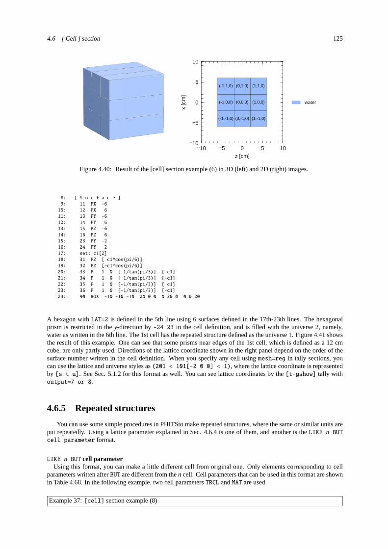
4.6 [ Cell ] section 125
0 5 10 15 20
0
5
10
15
20
−10 −5 0 5 10−10
−5
0
5
10
z [cm]
x [c
m]
water
(-1,-1,0) (0,-1,0) (1,-1,0)
(-1,0,0) (0,0,0) (1,0,0)
(-1,1,0) (0,1,0) (1,1,0)
Figure 4.40: Result of the [cell] section example (6) in 3D (left) and 2D (right) images.
8: [ S u r f a c e ]
9: 11 PX -6
10: 12 PX 6
11: 13 PY -6
12: 14 PY 6
13: 15 PZ -6
14: 16 PZ 6
15: 23 PY -2
16: 24 PY 2
17: set: c1[2]
18: 31 PZ [ c1*cos(pi/6)]
19: 32 PZ [-c1*cos(pi/6)]
20: 33 P 1 0 [ 1/tan(pi/3)] [ c1]
21: 34 P 1 0 [ 1/tan(pi/3)] [-c1]
22: 35 P 1 0 [-1/tan(pi/3)] [ c1]
23: 36 P 1 0 [-1/tan(pi/3)] [-c1]
24: 90 BOX -10 -10 -10 20 0 0 0 20 0 0 0 20
A hexagon withLAT=2 is defined in the 5th line using 6 surfaces defined in the 17th-23th lines. The hexagonalprism is restricted in they-direction by-24 23 in the cell definition, and is filled with the universe 2, namely,water as written in the 6th line. The 1st cell has the repeated structure defined as the universe 1. Figure4.41showsthe result of this example. One can see that some prisms near edges of the 1st cell, which is defined as a 12 cmcube, are only partly used. Directions of the lattice coordinate shown in the right panel depend on the order of thesurface number written in the cell definition. When you specify any cell usingmesh=reg in tally sections, youcan use the lattice and universe styles as(201 < 101[-2 0 0] < 1), where the lattice coordinate is representedby [s t u]. See Sec.5.1.2for this format as well. You can see lattice coordinates by the[t-gshow] tally withoutput=7 or 8.
4.6.5 Repeated structures
You can use some simple procedures in PHITSto make repeated structures, where the same or similar units areput repeatedly. Using a lattice parameter explained in Sec.4.6.4is one of them, and another is theLIKE n BUTcell parameter format.
LIKE n BUT cell parameterUsing this format, you can make a little different cell from original one. Only elements corresponding to cell
parameters written afterBUT are different from then cell. Cell parameters that can be used in this format are shownin Table4.68. In the following example, two cell parametersTRCL andMAT are used.
Example 37:[cell] section example (8)

126 4 SECTIONS FORMAT
0 5 10 15 20
0
5
10
15
20
−10 −5 0 5 10−10
−5
0
5
10
z [cm]
x [c
m]
water
(-1,-2,0) (0,-2,0) (1,-2,0) (2,-2,0) (3,-2,0)
(-1,-1,0) (0,-1,0) (1,-1,0) (2,-1,0)
(-1,0,0) (0,0,0) (1,0,0)(-2,0,0) (2,0,0)
(-2,1,0) (-1,1,0) (0,1,0) (1,1,0)
(-2,2,0) (-1,2,0) (0,2,0)(-3,2,0) (1,2,0)
Figure 4.41: Result of the [cell] section example (7) in 3D (left) and 2D (right) images.
1: [ M a t e r i a l ]
2: mat[1] 1H 2 16O 1
3: mat[2] Fe 1
4: [ C e l l ]
5: 1 0 -10 13 -14 #2 #3 #4
6: 2 1 1.0 11 -12 13 -14 15 -16
7: 3 LIKE 2 BUT TRCL=1
8: 4 LIKE 2 BUT TRCL=2 MAT=2
9: 5 -1 #(-10 13 -14)
10: [ S u r f a c e ]
11: 10 CY 10
12: 11 PX -2
13: 12 PX 2
14: 13 PY -2
15: 14 PY 2
16: 15 PZ -2
17: 16 PZ 2
18: [T r a n s f o r m ]
19: *tr1 3 0 -5
20: *tr2 0 0 6 30 90 120 90 0 90 60 90 30 1
A 4 cm cube filled with water is defined in the 6th line, and is put at the origin of the coordinate system. Insideof this cube is the 2nd cell regarded as the original cell in this example. In the 7th and 8th lines, respectively,the 3rd and 4th cells are defined with theLIKE n BUT format, wheren = 2. Figure4.42 shows the result ofthe example. The coordinate system of the 3rd cell is transformed using the cell parameterTRCL=1, where thecoordinate transform number 1 is defined in the 19th line in the[transform] section. That of the 4th cell is alsotransformed withTRCL=2. Moreover, the material inside of the cell is replaced with iron defined as the materialnumber 2 in the 3rd line.
−10 −5 0 5 10−10
−5
0
5
10
z [cm]
x [c
m] void
iron
water
1
42
3
Figure 4.42: Result of the [cell] section example (8).

4.6 [ Cell ] section 127
Nesting structure with latticeA nesting structure can be used on the basis of universe frame in Sec.4.6.3. For example, the universe 1 is
filled with the universe 2, and the universe 2 is filled with the universe 3. Moreover, the 3rd can be also filled withanother universe. Then, you can define the nesting structure. The maximum number of the nesting level is 10,which corresponds to a parametermxlv given in a fileparam.inc.
In the next example, there are nine square poles defined withLAT=1, and three of these have a different structurefrom the others.
Example 38:[cell] section example (9)
1: [ M a t e r i a l ]
2: mat[1] 1H 2 16O 1
3: mat[2] Fe 1
4: [ C e l l ]
5: 1 0 11 -12 13 -14 15 -16 FILL=1
6: 101 0 -26 25 -22 21 LAT=1 U=1
7: FILL=-1:1 -1:1 0:0
8: 2 2 3 2 3 2 3 2 2
9: 201 1 1.0 -90 U=2
10: 301 2 10.0 -10 U=3
11: 302 0 10 U=3
12: 2 -1 #1
13: [ S u r f a c e ]
14: 10 CY 1.5
15: 11 PX -6
16: 12 PX 6
17: 13 PY -6
18: 14 PY 6
19: 15 PZ -6
20: 16 PZ 6
21: 21 PX -2
22: 22 PX 2
23: 25 PZ -2
24: 26 PZ 2
25: 90 BOX -10 -10 -10 20 0 0 0 20 0 0 0 20
Definition of the 1st cell and the unit of lattice in the 5th and 6th lines, respectively, is the same of that in the[cell] section example (6). However, a format of the cell parameterFILL written in the 7th and 8th linesis different. In the 7th line, regions treated in this calculation are given in the lattice coordinate system. Thenumbers in the next line correspond to the universe number filling each lattice at (s, t,u), where the order is(−1,−1,0), (0,−1,0), (1,−1,0), (−1,0,0), . . . , (1,1,0); i.e., a lattice at (−1,−1,0) is filled with the universe 2 andthat at (1,−1,0) is filled with the universe 3. The universe 2 is defined in the 9th line as space filled with water.On the other hand, the universe 3 defined in the 10th and 11th lines has an iron cylinder at the origin. The result ofthis example is shown in Fig.4.43. One can see that three lattices at (1,−1,0), (0,0,0), and (−1,1,0) have the ironcylinder. When you specify any cell usingmesh=reg in tally sections, you can use the lattice and universe stylesas(302 < 101[0 0 0] < 1), where the lattice coordinate is represented by[s t u]. See also Sec.5.1.2forthis format.
−10 −5 0 5 10−10
−5
0
5
10
z [cm]
x [c
m] water
void
iron
(-1,-1,0) (0,-1,0)
(1,-1,0)
(1,-1,0)
(-1,0,0)
(0,0,0)
(1,0,0)(0,0,0)
(-1,1,0)
(0,1,0) (1,1,0)(-1,1,0)
Figure 4.43: Result of the [cell] section example (9).

128 4 SECTIONS FORMAT
More complex example is shown below.
Example 39:[cell] section example (10)
1: [ M a t e r i a l ]
2: mat[1] 1H 2 16O 1
3: mat[2] Fe 1
4: [ C e l l ]
5: 1 0 11 -12 13 -14 15 -16 FILL=1
6: 101 0 -26 25 -22 21 LAT=1 U=1
7: FILL=-1:1 -1:1 0:0
8: 2 2 3(1 0 1) 2 3(1 0 1) 2 3(1 0 1) 2 2
9: 201 1 1.0 -90 U=2
10: 301 0 -36 35 -32 31 LAT=1 U=3
11: FILL=-1:0 -1:0 0:0
12: 4 2 2 4
13: 401 2 10.0 -10 U=4
14: 402 0 10 U=4
15: 2 -1 #1
16: [ S u r f a c e ]
17: 10 CY 0.5
18: 11 PX -6
19: 12 PX 6
20: 13 PY -6
21: 14 PY 6
22: 15 PZ -6
23: 16 PZ 6
24: 21 PX -2
25: 22 PX 2
26: 25 PZ -2
27: 26 PZ 2
28: 31 PX -1
29: 32 PX 1
30: 35 PZ -1
31: 36 PZ 1
32: 90 BOX -10 -10 -10 20 0 0 0 20 0 0 0 20
The virtual space made by this input is shown in Fig.4.44. The nine square poles are defined with the latticeparameter. Furthermore, three of these consist of 4 units of the other lattice. The(1 0 1) in the 8th line denotesthe transformation of the coordinate system that the origin is shifted by 1cm in thex- andz-direction. When youspecify any cell usingmesh=reg in tally sections, you can use the lattice and universe styles as(402 < 301[-1
-1 0] < 101[0 0 0] < 1), where the lattice coordinate is represented by[s t u]. See also Sec.5.1.2for thisformat.
−10 −5 0 5 10−10
−5
0
5
10
z [cm]
x [c
m] water
void
iron
Figure 4.44: Result of the [cell] section example (10).

4.6 [ Cell ] section 129
Voxel phantomIn PHITS, you can make a virtual space using voxel phantom for calculation on complex structures, such as
the human body or organism. First, a little cube is defined as a unit of the lattice withLAT=1. Second, you set arepeated structure of a large size using the unit. Third, you fill each unit with any universe, which is itself filledwith biological matter, such as compounds of carbon and water.
In an example below, a 10 cm cube consisting of 2cm cubes (voxels) of 5× 5× 5 = 125 is described.
Example 40:[cell] section example (11)
1: [ M a t e r i a l ]
2: mat[1] 1H 2 16O 1
3: mat[2] Fe 1
4: [ C e l l ]
5: 1 0 11 -12 13 -14 15 -16 FILL=1
6: 101 0 -20 LAT=1 U=1
7: FILL=-2:2 -2:2 -2:2
8: 2 2 2 2 2 2 2 2 2 2 2 2 3 2 2 2 2 2 2 2 2 2 2 2 2
9: 2 2 2 2 2 2 3 3 2 2 2 3 4 3 2 2 3 3 2 2 2 2 2 2 2
10: 2 2 2 2 2 2 3 3 3 2 3 4 4 4 3 2 3 3 3 2 2 2 2 2 2
11: 2 2 2 2 2 2 2 3 3 2 2 3 4 3 2 2 2 3 3 2 2 2 2 2 2
12: 2 2 2 2 2 2 2 2 2 2 2 2 3 2 2 2 2 2 2 2 2 2 2 2 2
13: 201 0 -90 U=2
14: 301 2 10.0 -90 U=3
15: 401 1 1.0 -90 U=4
16: 2 -1 #1
17: [ S u r f a c e ]
18: 11 PX -5
19: 12 PX 5
20: 13 PY -5
21: 14 PY 5
22: 15 PZ -5
23: 16 PZ 5
24: 20 BOX -1 -1 -1 2 0 0 0 2 0 0 0 2
25: 90 BOX -10 -10 -10 20 0 0 0 20 0 0 0 20
As a unit of voxel, a 2 cm cube is defined in the 24th line. Furthermore, the 1st cell that is inside of a 10 cm cube hasa repeated structure through definition in the 5th line. The region of the lattice coordinate space is determined in the7th line. The order of voxel in the 8th-12th lines is as follows: (−2,−2,−2), (−1,−2,−2), . . . , (2,2,2) representedby the lattice coordinate.2 in the 8th-12th lines means the universe 2, which is void, and3 and4, namely theuniverse 3 and 4, correspond to iron and water, respectively. Figure4.45represents the result of this example thatis a distorted iron box including water its inside. When you specify any cell usingmesh=reg in tally sections, youcan use the lattice and universe styles as(401 < 101[0 0 0] < 1), where the lattice coordinate is representedby [s t u]. See also Sec.5.1.2for this format. It is noted that you cannot use formats as(301 < 101[-2:2-2:2 -2:2] < 1) because not all the101[-2:2 -2:2 -2:2] cell have the 301st cell.
0 5 10 15 20
0
5
10
15
20
0 5 10 15 20
0
5
10
15
20
Figure 4.45: Results of the [cell] section example (11) in 3D images. The structure in the right panel is removedits iron surface from the original one in the left panel.

130 4 SECTIONS FORMAT
For time shortening, you can useivoxel in the[parameters] section. When you perform PHITS calculationwith ivoxel=2, voxel data are output infile(18) in binary and then the calculation is stopped. From the nextcalculation withivoxel=1, a process of the data output is omitted and the calculation time is shortened. If youuse a very huge voxel data, usinginflmay become to be convenient.
Use of tetrahedron geometryIn this section, definition and basic usage of tetrahedron geometry are explained showing an example. Tetrahe-
dron geometry is a type of polygon mesh geometry and is able to express complex geometry by combination ofdifferent size of tetrahedrons.
Tetrahedron geometry is represented by two files:
• Node file (List of xyz space coordinates of tetrahedron nodes).
• Element file (List of 4 nodes’IDs consisting each tetrahedron element).
PHITS postulates that the node file and the element file have a common name with different suffixes, .node and.ele, respectively. Please see ppt file or sample input file in\phits\utility\TetraGEOM in detail.
An example of the node file and the element file is given below.
Example 41: Example of node file
1: # Simple two elements
2: 5 3 0 0
3: # pointID x y z
4: 1 0.0 -2.5 -4.0
5: 2 -4.0 -2.5 0.0
6: 3 4.0 -2.5 0.0
7: 4 0.0 -2.5 4.0
8: 5 0.0 2.5 0.0
The node file begins with the number of nodes and the number of dimensions (2nd line). PHITS can deal with onlythree-dimensional geometry. The two last zeros in the 2nd line are not used in PHITS. The following lines (below3rd line) represent a list of nodes and their xyz space coordinates in the order of
[node no.] [x] [y] [z]
Example 42: Example of element file
1: # Simple two elements
2: 2 4 1
3: # elementID point(1:4) universe
4: 1 1 2 3 5 5001
5: 2 5 2 3 4 5002
The element file begins with the number of elements, the number of nodes consisting a tetrahedron (=4 for PHITS),and the number of information tagged to an element (=1 for PHITS) [2nd line]. The following lines (below 3rdline) represent a list of IDs of 4 nodes consisting each tetrahedron in the order of
[element no.] [node 1] [node 2] [node 3] [node4] [element universe no.]
The element no. represents the ID of the tetrahedron element. The list of IDs of 4 nodes are specified by the nodeNo. given in the node file. The element universe no. specifies the universe to fill this tetrahedron element. Thedefinition of this universe should be given in the PHITS input file (See Example43). Arbitrary comment linesstarting with “#” can be inserted in any line of the node file and the element file.
The node file and the element file can be created by using a software, Tetrahedral Mesh Generator (TetGen).By using this software, general polygon mesh data can be converted to tetrahedron geometry with some effort.TetGen can be obtained from
http://wias-berlin.de/software/tetgen/

4.6 [ Cell ] section 131
with free of charge. For details of TetGen, please refer to its manual.The way to specify the use of tetrahedron geometry in PHITS input file is explained in below.
Example 43:[cell] section example (12)
1: [Material]
2: mat[1] 14N 78.1 16O 20.9 40Ar 0.93
3: mat[2] 1H 2 16O 1
4: mat[3] 56Fe 1
5: [Surface]
6: 10 rpp -5.0 5.0 -3.0 3.0 -5.0 5.0
7: 20 rpp -7.0 7.0 -5.0 5.0 -7.0 7.0
8: 90 so 500.0
9: [Cell]
10: 101 1 -0.001205 -20 U=1 LAT=3 tfile=Tetra TSFAC=1.0
11: 1 0 -10 FILL=1
12: 2 -1 10
13: 201 2 -1.0 -90 U=5000
14: 202 3 -7.874 -90 U=5001
Element 1
Element 2
Node 1
Node 2
Node 3
Node 4
Node 5
Figure 4.46: Results of the [cell] section ex-ample (11) in 3D images.
A region defined in rectangular shape (with surface symbol RPP)is required and tetrahedron geometry will be expanded in this re-gion. This region should contain all the nodes of tetrahedronsbut should not be too large to avoid unnecessary computationalcosts. At 10th line, a region with cell no. 101 is defined by arectangular shape specified by surface number 20, a rectangularbox of 14cm×10cm×14cm, the optionLAT=3 declares the use oftetrahedron geometry. Tetrahedron geometry defined by the nodefile and the element file with the name specified byTFILE is ex-panded in this region. Here it should be noted that upper andlower cases of the file name are distinguished for Mac and Linux.With the factorTSFAC, the size of tetrahedron geometry can bescaled-up or scaled-down. The factor will be multiplied to thecoordinates of nodes. The material given in the cell 101 is usedto fill the region 101 except for inside of tetrahedrons. In 11thline, the region with cell no. 1 is defined as a rectangular box of10cm×6cm×10cm. With theFILL option, this region is filled bythe cell no. 101 containing tetrahedron geometry. Tetrahedrongeometry (LAT=3) should be used together with universe&fill nest structure in the same way as Lattice structurelike this example. The universes appeared in the element file should be defined in the same way as the Latticestructure, which is done in Line 13 and 14 for this example. The element no. 1 is filled by the material 2, water(H2O), and the element no. 2 is filled by the material 3, iron (Fe).

132 4 SECTIONS FORMAT
4.7 [ Transform ] section
4.7.1 Formats
You can define the coordinate transform in this section. OnlyC and$ can be used as a comment mark. Fileincluding and variable definition can be set in this section. You can only rotate and/or transport the coordinate, andcannot enlarge or shrink using[transform].
The coordinate transformation defined in this section can be used in[source] section,[surface] section,[cell] section,r-z, xyz mesh of tally and the magnetic field.
Formats and examples are shown below.
[ T r a n s f o r m ]
TRn O1 O2 O3 B1 B2 B3 B4 B5 B6 B7 B8 B9 M
Table 4.69:transform definition
item explanation
n transform number 1∼ 999999∗TRn means thatBi is not a cosine, but an angle (degree).
O1 O2 O3 transposition vectorB1 ∼ B9 rotation matrix
You can define only rotation matrix. The determinant of the matrix isautomatically adjusted to 1.
M = 1 means that transposition vector is in sub coordinate systemdefined in main coordinate system.= −1 means that transposition vector is in main coordinate systemdefined in sub coordinate system.
Default values are shown below.
TRn 0 0 0 1 0 0 0 1 0 0 0 1 1
4.7.2 Mathematical definition of the transform
The mathematical definition in terms of transposition vector and rotation matrix is the following,In the case ofM = 1, x′
y′
z′
= B1 B2 B3
B4 B5 B6
B7 B8 B9
x
yz
+ O1
O2
O3
In the case ofM = −1, x′
y′
z′
= B1 B2 B3
B4 B5 B6
B7 B8 B9
x
yz
− B1 B4 B7
B2 B5 B8
B3 B6 B9
O1
O2
O3

4.7 [ Transform ] section 133
Here,
B1 = cos(x′, x)
B2 = cos(x′, y)
B3 = cos(x′, z)
B4 = cos(y′, x)
B5 = cos(y′, y)
B6 = cos(y′, z)
B7 = cos(z′, x)
B8 = cos(z′, y)
B9 = cos(z′, z)
In the case ofM = 1, the object used this transform function is rotated and then translated. On the other hand, inthe case ofM = −1, the rotation is performed after the translation. The rotation is performed about the origin ofthexyzcoordinate system. Note that the direction of the translation settingM = 1 and−1 is opposite each other.
4.7.3 Examples (1)
Example 44:[transform] section example (1)
1: [ T r a n s f o r m ]
2: *tr1 0.0000000E+00 0.0000000E+00 1.4000000E+03
3: 1.3500000E+02 9.0000000E+01 4.5000000E+01
4: 9.0000000E+01 0.0000000E+00 9.0000000E+01
5: 2.2500000E+02 9.0000000E+01 1.3500000E+02 1
6: *tr2 0.0000000E+00 0.0000000E+00 2.5800000E+03
7: 3.0000000E+02 9.0000000E+01 2.1000000E+02
8: 9.0000000E+01 0.0000000E+00 9.0000000E+01
9: 3.0000000E+01 9.0000000E+01 3.0000000E+02 1
In this example,tr1 rotates the coordinate by 135 degrees aroundy axis, and transports 140 cm tozdirection,while tr2 rotates 300 degrees aroundy axis, and transports 258 cm tozdirection. Because ofTRn with ∗, you cangive angles (in units of degree) directly forBi , (i = 1, . . . ,9).
4.7.4 Examples (2)
Example 45:[transform] section example (2)
1: [ T r a n s f o r m ]
2: set: c10[90] $ angle of around Z (degree)
3: set: c20[30] $ angle of around Y (degree)
4: set: c30[0] $ angle of around X (degree)
5:
6: tr1 0 0 0
7: cos(c10/180*pi)*cos(c20/180*pi)
8: sin(c10/180*pi)*cos(c30/180*pi)+cos(c10/180*pi)*sin(c20/180*pi)*sin(c30/180*pi)
9: sin(c10/180*pi)*sin(c30/180*pi)-cos(c10/180*pi)*sin(c20/180*pi)*cos(c30/180*pi)
10: -sin(c10/180*pi)*cos(c20/180*pi)
11: cos(c10/180*pi)*cos(c30/180*pi)-sin(c10/180*pi)*sin(c20/180*pi)*sin(c30/180*pi)
12: cos(c10/180*pi)*sin(c30/180*pi)+sin(c10/180*pi)*sin(c20/180*pi)*cos(c30/180*pi)
13: sin(c20/180*pi)
14: -cos(c20/180*pi)*sin(c30/180*pi)
15: cos(c20/180*pi)*cos(c30/180*pi)
16: 1
In this example, tr1 rotates the coordinate by c10 degree around z axis, c20 degree around y axis and finallyc30 degree around x axis. You can set c10, c20, c30, and rotate the coodinate to any direction as you want.

134 4 SECTIONS FORMAT
4.8 [ Temperature ] section
Free-Gas Thermal Temperature (MeV) for GG cell can be defined in this section. This section corresponds toTMP card but you cannot set time definition. This value can be set in the[cell] section when you use GG. If thetemperature is double defined, temperatures defined in this[temperature] sections are used. If you do not setthis, the default value is 2.53× 10⁻⁸MeV.
[ T e m p e r a t u r e ]
reg tmp
1 1.0*1.e-8
11 5.0*1.e-8
( 2 - 5 8 9 ) 2.0*1.e-8
( 11 12 15 ) 3.0*1.e-8
16 6.0*1.e-8
.... ........
.... ........
You can use the format( 2 - 5 8 9 ). In this case, you need to close a value by( ) , if it is not asingle numeric value.
You cannot use the lattice and universe style as( 6 < 10[1 0 0] < u=3 ).If you want to change the order of region number (reg) and temperature (tmp), you can set as “tmp reg”.
You can use the skip operatornon. Even if you use GG, you should write the symbol notcell butreg here.

4.9 [ Mat Time Change ] section 135
4.9 [ Mat Time Change ] section
By this section, you can change the material of certain cells to the other material as a function of time. Thisfunction is useful to describe a shutter of beam line, T0 chopper and the other devices for neutron optics. The unitof time is nsec.
[ Mat Time Change ]
mat time change
1 50.0 11
2 100.0 12
3 1000.0 0
.... ........
.... ........
In the above example, the material 1 is changed to material 11 at t=50.0 nsec, 2 to 12 at 100 nsec and 3 to voidat 1000 nsec. If you want to replace the order of the initial material (mat), time (time) and the final material(change), set as ”mat change time”. You can use the skip operatornon. These three columns are alwaysnecessary to define the mat time change function.

136 4 SECTIONS FORMAT
4.10 [ Magnetic Field ] section
4.10.1 Charged particle
You can set a magnetic field in the PHITS calculation. If you use this function for electron and positron, setEGS5 mode.
Cell number (reg), magnetic field type (typ), half distance of magnets (gap)(cm), magnetic field intensity(mgf), transformation (trcl) and time dependence (time) should be defined as
[ Magnetic Field ]
reg typ gap mgf trcl time
1 4 10.00000 -5.956540 3 non
2 4 10.00000 6.416140 1 non
3 2 10.00000 -7.611980 0 0.0
4 2 10.00000 3.516000 0 pi/2
( 150 < 61 ) 4 13.00000 7.880140 2 non
( 150 < 62 ) 4 13.00000 -7.440800 2 non
( 150 < 63 ) 4 13.00000 9.441010 2 non
( 150 < 64 ) 4 13.00000 -8.295220 2 non
( 150 < 65 ) 4 13.00000 3.694830 2 non
( 150 < 66 ) 4 13.00000 -2.099350 2 non
... ... ........ ........ ... ...
... ... ........ ........ ... ...
The column oftrcl is omissible. The zero for trcl means no transformation. Thetime is a parameter of userdefined time dependent magnetic field. The column oftime is also omissible. The “non” for time means no timedependence. Two subroutines, usrmgt1.f and usrmgt2.f are included in the source as user defined subroutines forthe time dependent magnetic field. The former is for Wobbler magnet, and the latter is for pulse magnet for neutronoptics. You can choose these two subroutine by usrmgt=1, 2 in the parameter section. For the Wobbler magnet,“time” means phase of the magnet, starting time for pulse magnet, respectively.
In the above expression,reg is region number,typ can take2 or 4 for dipole electromagnet, or quadrupoleelectromagnet respectively. mgf denotes the strength of the magnetic field (kG), andtrcl is the coordinatetransformation number defined in[transform] section.
You can use the format( 2 - 5 8 9 ), and you can use the lattice and universe style as( 6 < 10[1 0 0] < u=3 ). But you need to close a value by( ) if it is not a single numeric value.
By using this format, you can set different magnetic field for each lattice. If a cell is re-defined, the value,which is defined at first, is used.
In the case of dipole magnet, the distancesgap make no sense, but set any numeric. The magnetic field isavailable not only in the void region, but also in the material where the normal reaction can be occurred.
z-axis is assumed to be the center of the magnetic field. The direction of the magnetic field is positive directionof y-axis for dipole, i.e. the positive charge particle is bent to positive direction of x-axis when it goes to positivedirection of z-axis. For quadrupole, the positive particle is converged in x-axis, diverged in y-axis when it goes topositive direction of z-axis. You need the coordinate transformation bytrcl for different geometrical situation.
When you specify charge number of the projectile particle withizst in [source] section, the motion of theparticle with the number in the magnetic field is described. Usingizst, PHITS can simulate the motion of theparticle with charge states. The charge number defined withizst doesn’t change while the particle moves. Itshould be noted that particles produced from nuclear reactions are not affected by the value ofizst; the charge ofthe produced particle is given as its atomic number.
Normally, the tallies are called at the reaction point or the surface crossing; thus, the particle track in, forexample, the magnetic field is shown as a straight line between collisions or between one collision and a surfacecrossing. To describe the trajectory correctly as a curve, setitstep=1 and adjust the step length for the field bydeltm in [parameters].

4.10 [ Magnetic Field ] section 137
4.10.2 Neutron
The definition of the magnetic field for neutron is almost the same as for charged particles. Here we describethe detail of the magnetic field for neutron.
[ Magnetic Field ]
reg typ gap mgf trcl polar time
1 60 0.00000 35000.0 3 non non
2 61 0.00000 35000.0 1 1 non
3 106 5.00000 7130.0 0 0 non
4 104 0.00000 3.5 0 non 5.0
5 102 0.00000 0.20 0 non non
6 101 3.00000 7130.0 2 1 non
7 103 0.00000 35000.0 0 -1 non
... ... ........ ........ ... ... ...
... ... ........ ........ ... ... ...
We cannot take into account of the gravity nor additional dipole magnet. For60 case, it is assumed that the spinalways keeps parallel or anti-parallel to the magnet field. For61 case, we solve the coupled equation of motionbetween the spin and the magnetic field. Then the spin flip can be occurred in the region with weak magnetic field.The strength of the magnetic field is specified in the unit of [T/m2] in mgf column.
For the types above 100, we consider the coupled equations of the spin and the magnetic field. In addition, theeffects of the gravity and additional dipole field can be taken into account.106 is sextupole,104 quadrupole, and102 dipole, respectively. The strength of additional quadrupole magnet (z-direction) is give by the column of gapin the unit of [T].
For 101 type, the magnetic field is defined by the user program file, usrmgf1.f. In this user program, the datameasured by the neutron optics group in JAERI are read from the file and used the calculation. The strength of thisfield is renormalized by the value of mgf.
For101 type, the magnetic field is also defined by the user program file, usrmgf3.f. In this user program, thereis a simple sextupole magnet field as same as in106 type.
The neutron goes into the magnetic field with the initial spin if it is defined in the source section. If not, theinitial spin is defined at the moment when the neutron goes into the magnetic field. The ratio of the number ofparallel and anti-parallel spin to the magnetic field is determined by the polarization defined by thepolar column.non in polar column means 0 polarization. The polarization is defined as
P =ϕ+ − ϕ−ϕ+ + ϕ−
,
here,ϕ+ andϕ− are the number of the parallel and anti-parallel particles.
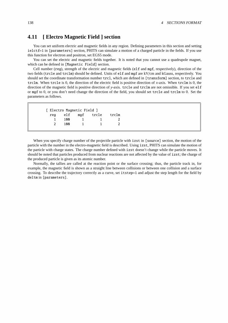
138 4 SECTIONS FORMAT
4.11 [ Electro Magnetic Field ] section
You can set uniform electric and magnetic fields in any region. Defining parameters in this section and settingielctf=1 in [parameters] section, PHITS can simulate a motion of a charged particle in the fields. If you usethis function for electron and positron, set EGS5 mode.
You can set the electric and magnetic fields together. It is noted that you cannot use a quadrupole magnet,which can be defined in[Magnetic Field] section.
Cell number (reg), strength of the electric and magnetic fields (elf andmgf, respectively), direction of thetwo fields (trcle andtrclm) should be defined. Units ofelf andmgf are kV/cm and kGauss, respectively. Youshould set the coordinate transformation numbertrcl, which are defined in[transform] section, totrcle andtrclm. Whentrcle is 0, the direction of the electric field is positive direction ofx-axis. Whentrclm is 0, thedirection of the magnetic field is positive direction ofy-axis. trcle andtrclm are not omissible. If you setelfor mgf to 0, or you don’t need change the direction of the field, you should settrcle andtrclm to 0. Set theparameters as follows.
[ Electro Magnetic Field ]
reg elf mgf trcle trclm
1 100 1 1 2
2 100 1 1 2
When you specify charge number of the projectile particle withizst in [source] section, the motion of theparticle with the number in the electro-magnetic field is described. Usingizst, PHITS can simulate the motion ofthe particle with charge states. The charge number defined withizst doesn’t change while the particle moves. Itshould be noted that particles produced from nuclear reactions are not affected by the value ofizst; the charge ofthe produced particle is given as its atomic number.
Normally, the tallies are called at the reaction point or the surface crossing; thus, the particle track in, forexample, the magnetic field is shown as a straight line between collisions or between one collision and a surfacecrossing. To describe the trajectory correctly as a curve, setitstep=1 and adjust the step length for the field bydeltm in [parameters].
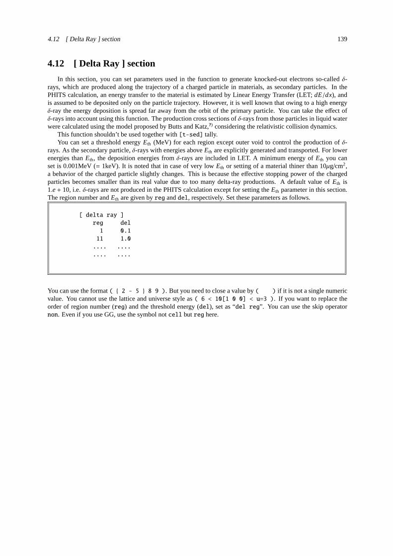
4.12 [ Delta Ray ] section 139
4.12 [ Delta Ray ] section
In this section, you can set parameters used in the function to generate knocked-out electrons so-calledδ-rays, which are produced along the trajectory of a charged particle in materials, as secondary particles. In thePHITS calculation, an energy transfer to the material is estimated by Linear Energy Transfer (LET;dE/dx), andis assumed to be deposited only on the particle trajectory. However, it is well known that owing to a high energyδ-ray the energy deposition is spread far away from the orbit of the primary particle. You can take the effect ofδ-rays into account using this function. The production cross sections ofδ-rays from those particles in liquid waterwere calculated using the model proposed by Butts and Katz,?) considering the relativistic collision dynamics.
This function shouldn’t be used together with[t-sed] tally.You can set a threshold energyEth (MeV) for each region except outer void to control the production ofδ-
rays. As the secondary particle,δ-rays with energies aboveEth are explicitly generated and transported. For lowerenergies thanEth, the deposition energies fromδ-rays are included in LET. A minimum energy ofEth you canset is 0.001MeV (= 1keV). It is noted that in case of very lowEth or setting of a material thiner than 10µg/cm2,a behavior of the charged particle slightly changes. This is because the effective stopping power of the chargedparticles becomes smaller than its real value due to too many delta-ray productions. A default value ofEth is1.e+ 10, i.e.δ-rays are not produced in the PHITS calculation except for setting theEth parameter in this section.The region number andEth are given byreg anddel, respectively. Set these parameters as follows.
[ delta ray ]
reg del
1 0.1
11 1.0
.... ....
.... ....
You can use the format( 2 - 5 8 9 ). But you need to close a value by( ) if it is not a single numericvalue. You cannot use the lattice and universe style as( 6 < 10[1 0 0] < u=3 ). If you want to replace theorder of region number (reg) and the threshold energy (del), set as “del reg”. You can use the skip operatornon. Even if you use GG, use the symbol notcell butreg here.

140 4 SECTIONS FORMAT
4.13 [ Track Structure ] section
Performing the track-structure simulation42 for electrons or positrons of low energy below 1 keV, those decel-eration processes caused by much collision events for ionization, excitation, and molecular vibration and rotationcan be calculated precisely. Currently, the cross sections only for liquid water are prepared in PHITS, and thosefor other materials are simply obtained from electron density scaling based on the data. The track-structure simu-lation takes so long time that we cannot recommend to activate this mode in a conventional-scale particle transportsimulation (cm orders) due to much production of low energy electrons around 10 eV. Please take cares that thetrack-structure mode can be adapted only to[t-track] and[t-deposit] tallies.
In this section, you have to specify the cells where you would like to perform track-structure simulation.mID
represents the index of the cross sections database used in the track-structure simulation, and currently you canselect only 0 (no track structure simulation) or 1 (track structure simulation using the database of liquid water). Ifyou will activatemID = 1, mean free paths of the particles in target materials are derived from electron densityscaling based on the database for liquid water. We are planning to prepare the cross section databases for othermaterials in future.
[track structure]
reg mID
1 1
2 0
You can use the format( 2 - 5 89 ). But you need to close a value by( ) if it is not a single numericvalue. You cannot use the lattice and universe style as( 6 < 10[100] < u=3 ). If you want to replace theorder of region number (reg) and index of the cross section database (mID), set asmID reg. You can use the skipoperatornon.
The followings are the important parameters for this mode. The parameters ofetsmax andetsmin in [parameters]section are maximum and minimum energies of particles simulated by track-structure mode. In case of the useof the track-structure mode, the parameters ofemin(12) andemin(13) should be set concurrently to 1.0e-3, andEGS5 should be activated (negs=1).
[ P a r a m e t e r s ]
emin(12) = 1.E-03
emin(13) = 1.E-03
negs = 1
etsmax = 1.E-2
etsmin = 1.E-6
42 T. Kai et al.,“ Thermal equilibrium and prehydration processes of electrons injected into liquid water calculated by dynamic Monte Carlomethod”, Radiat. Phys. Chem., 115, 1-5 (2015).

4.14 [ Super Mirror ] section 141
4.14 [ Super Mirror ] section
The reflection of low energy neutron by super mirror is defined by this section. We assume the followingempirical formula to describe the reflectivity of the super mirrors.
R=
R0 if Q ≤ Qc12R0 (1− tanh [(Q−mQc)/W]) (1− α(Q− Qc)) if Q > Qc
whereQ is the scattering vector (in Å−1) defined by
Q = |k i − k f | =4π sinθλ
.
The value ofm is a parameter determined by the mirror material, the bilayer sequence and the number of bilayers.Qc is the critical scattering wave vector for a single layer of the mirror material. At higher values ofQ, thereflectivity starts falling linearly with a slopeα until a cutoff at Q = mQc. The width of the cutoff is denotedW.
These parameters are defined as
[ Super Mirror ]
r-in r-out mm r0 qc am wm
2001-2020 3001 3 0.99 0.0217 3.0 0.003
2500 3500 3 0.99 0.0217 3.0 0.003
2600 3600 3 0.99 0.0217 3.0 0.003
.... .... .. ... .... ... ...
.... .... .. ... .... ... ...
.... .... .. ... .... ... ...
The reflection surface is defined by the surface betweenr-in andr-out. You can use the format( 2 - 5 8 9 ), and you can use the lattice and universe style as( 6 < 10[1 0 0] < u=3 ) in these definitions. Theremaining parameters in above expression denotemby mm, R0 by r0, Qc by qc in Å−1, α by am in Å, andW by wmin Å−1.
We restrict this function only to neutrons for the case that its energy is less than 10 eV or sinθ is greater than0.001, the latter is due to roughness of the surface.
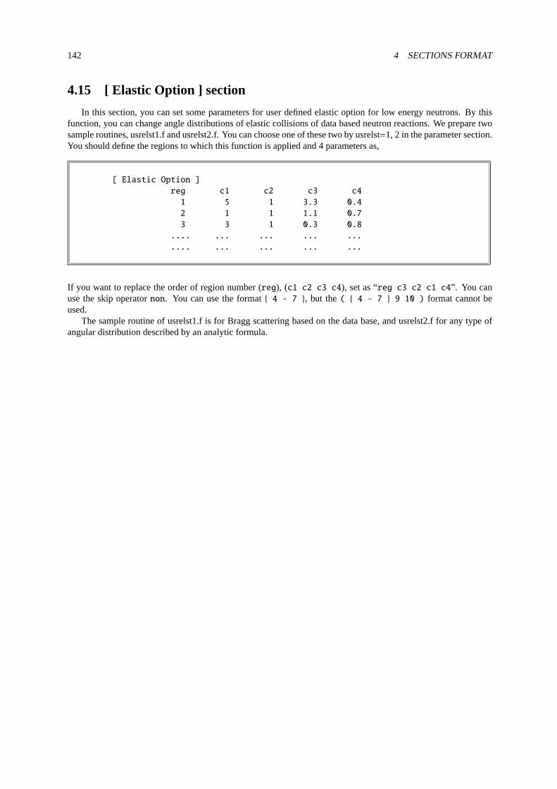
142 4 SECTIONS FORMAT
4.15 [ Elastic Option ] section
In this section, you can set some parameters for user defined elastic option for low energy neutrons. By thisfunction, you can change angle distributions of elastic collisions of data based neutron reactions. We prepare twosample routines, usrelst1.f and usrelst2.f. You can choose one of these two by usrelst=1, 2 in the parameter section.You should define the regions to which this function is applied and 4 parameters as,
[ Elastic Option ]
reg c1 c2 c3 c4
1 5 1 3.3 0.4
2 1 1 1.1 0.7
3 3 1 0.3 0.8
.... ... ... ... ...
.... ... ... ... ...
If you want to replace the order of region number (reg), (c1 c2 c3 c4), set as “reg c3 c2 c1 c4”. You canuse the skip operatornon. You can use the format 4 - 7 , but the( 4 - 7 9 10 ) format cannot beused.
The sample routine of usrelst1.f is for Bragg scattering based on the data base, and usrelst2.f for any type ofangular distribution described by an analytic formula.

4.16 [ Data Max ] section 143
4.16 [ Data Max ] section
dmax(i), which is the maximum energy of library use for i-th particle, can be defined for each nucleus inmaterials in this section. Maximum 6[Data Max] sections are allowed to be used in a input file.
[Data Max]
part = neutron proton
mat nucleus dmax
all Fe 20
5 all 50
3 56Fe 150
Particle is defined in the first line aspart =. Only neutron and proton can be define in PHITS ver. 2.86.Three columns,mat, nucleus, anddmax, can be used. If you want to change the order of (mat) (nucleus),
set as “nucleus mat”. You can use the skip operator non. In the mat column, material numbers can be specified andall means all materials. In the nucleus column, you can specify nucleus as 56Fe and 26056 type. You can use Feor 26000, which specifies all isotopes of Fe. You can also use all. By the number (MeV) in thedmax column, youdefine the maximum energy of library use for the nucleus.
If the same nucleus is defined in the[data max] sections, the latest definition has priority in an input file.The values ofdmax(1) anddmax(2) defined by[parameters] section should be the maximum value in
[data max] section.If kmout = 1 is specified in[parameters] section, the values of dmax for each nucleus in the materials are
shown in the output file,file(6) (D=phits.out).

144 4 SECTIONS FORMAT
4.17 [ Frag Data ] section
The function to read user defined cross sections can be defined in the[frag data] section. By using thisfunction, you can simulate nuclear reaction events in the calculation on the basis of information given by the crosssection data. It is noted that nuclear data libraries are preferentially used, even in the case of a nuclear reaction youspecify in this section. You can set only proton, neutron, and nuclei as incident particles. Photons and electionscannot be used. Elastic scattering events for nucleons are separately considered by the default model implementedin PHITS.
Because weight values of the secondary particles produced by this option change from 1.0, you should decreasethe value of the cutoff weight parameterwc2(i) in the[parameters] section.
Set the parameters as follows.
[ Frag Data ]
opt proj targ file
0 12C 16O DDX_12C-16O.dat
1 proton 63Cu DDX_p-63Cu.dat
.... ... ... ... ...
.... ... ... ... ...
The user defined cross sections are not used when opt=0. In the case of opt=1, PHITS reproduces the cross sectionof the reaction between an incident particle and target, which are specified by proj and targ, respectively, using thedata. Options when opt=2,3 are under construction. When opt=4, PHITS simply extrapolates the given data forincident energies, emission angles, and emission energies. Note that you can use this option only in the case ofneo>0 and nag,0, which will be explained below.
Format of the data of the user defined cross sections is as follows.
projectiletargetneiein(1) ein(2) ein(3) ...... ein(nei+1)totxs(1) totxs(2) totxs(3) ...... totxs(nei+1)neoeout(1) eout(2) eout(3) ...... eout(neo+1)nagangle(1) angle(2) angle(3) ...... angle(nag+1)nfrgfrag(1) frag(2) frag(3) ...... frag(nfrg)
proxs(1,1) proxs(1,2) proxs(1,3) ...... proxs(1,nfrg)ddx(1,1,1,1) ddx(1,1,1,2) ddx(1,1,1,3) ...... ddx(1,1,1,nag)ddx(1,1,2,1) ddx(1,1,2,2) ddx(1,1,2,3) ...... ddx(1,1,2,nag)
.........
ddx(1,1,neo,1) ddx(1,1,neo,2) ddx(1,1,neo,3) ...... ddx(1,1,neo,nag)
ddx(1,2,1,1) ddx(1,2,1,2) ddx(1,2,1,3) ...... ddx(1,2,1,nag)ddx(1,2,2,1) ddx(1,2,2,2) ddx(1,2,2,3) ...... ddx(1,2,2,nag)
.........
ddx(1,2,neo,1) ddx(1,2,neo,2) ddx(1,2,neo,3) ...... ddx(1,2,neo,nag)
.........
.........

4.17 [ Frag Data ] section 145
(continued)
ddx(1,nfrg,1,1) ddx(1,nfrg,1,2) ddx(1,nfrg,1,3) ...... ddx(1,nfrg,1,nag)ddx(1,nfrg,2,1) ddx(1,nfrg,2,2) ddx(1,nfrg,2,3) ...... ddx(1,nfrg,2,nag)
.........
ddx(1,nfrg,neo,1) ddx(1,nfrg,neo,2) ddx(1,nfrg,neo,3) ...... ddx(1,nfrg,neo,nag)
proxs(2,1) proxs(2,2) proxs(2,3) ...... proxs(2,nfrg)ddx(2,1,1,1) ddx(2,1,1,2) ddx(2,1,1,3) ...... ddx(2,1,1,nag)ddx(2,1,2,1) ddx(2,1,2,2) ddx(2,1,2,3) ...... ddx(2,1,2,nag)
.........
ddx(2,1,neo,1) ddx(2,1,neo,2) ddx(2,1,neo,3) ...... ddx(2,1,neo,nag)
.........
.........
.........
.........
proxs(nei+1,1) proxs(nei+1,2) proxs(nei+1,3) ...... proxs(nei+1,nfrg)ddx(nei+1,1,1,1) ddx(nei+1,1,1,2) ddx(nei+1,1,1,3) ...... ddx(nei+1,1,1,nag)ddx(nei+1,1,2,1) ddx(nei+1,1,2,2) ddx(nei+1,1,2,3) ...... ddx(nei+1,1,2,nag)
.........
ddx(nei+1,1,neo,1) ddx(nei+1,1,neo,2) ddx(nei+1,1,neo,3) ...... ddx(nei+1,1,neo,nag)
.........
.........
ddx(nei+1,nfrg,1,1) ddx(nei+1,nfrg,1,2) ddx(nei+1,nfrg,1,3) ...... ddx(nei+1,nfrg,1,nag)ddx(nei+1,nfrg,2,1) ddx(nei+1,nfrg,2,2) ddx(nei+1,nfrg,2,3) ...... ddx(nei+1,nfrg,2,nag)
.........
ddx(nei+1,nfrg,neo,1) ddx(nei+1,nfrg,neo,2) ddx(nei+1,nfrg,neo,3) ...... ddx(nei+1,nfrg,neo,nag)
In the beginning, you specify incident particle and target in this file. nei is the number of points of the energymesh. In the next line, you set nei+1 points of incident energies (ein in the unit of MeV/u). neo is the number ofenergy mesh points of the outgoing particles. In the next line, you set neo+1 points of the energy (eout in the unitof MeV/u), and then in the next next line you set neo+1 data of total reaction cross sections (totxs in the unit ofmb). Note that when totxs=0, total reaction cross sections obtained by models, which are specified byicxsni oricrhi, are used. nag is the number of angular mesh points for the outgoing particles. You set nag+1 data of theangles in the next line. If nag>0 the data should be given in the unit of radian, and if nag<0 those are in the unit isdegree. When nag=0, isotropic is assumed. nfrg is the number of the outgoing particles. In the next line, you writenfrg names of the particles. proxs (in the unit of mb) is the production cross sections of the particles at an incidentenergy, and then you set neo×nag data of the double differential cross sections (ddx in the unit of mb/MeV/sr).You have to specify nei+1 groups of the proxs and ddxs per an outgoing particle.
If you write model in the line where you should write neo, nuclear reaction models are used for simulatingnuclear reaction events. In this case, you do not have to write the data below neo.
Example 46: example of data file of user defined cross sections
1: proton
2: 63Cu
3: 1
4: 10.0 100.0
5: 1000.0 500.0
6: 3
7: 1.0 10.0 50.0 100.0
8: -6
9: 0.0 30.0 60.0 90.0 120.0 150.0 180.0

146 4 SECTIONS FORMAT
10: 1
11: neutron
12: 300.0
13: 10.0 10.0 10.0 10.0 10.0 10.0
14: 15.0 13.0 12.0 11.0 10.0 10.0
15: 10.0 11.0 10.0 11.0 10.0 10.0
16: 0.0
17: 5.0 5.0 5.0 5.0 5.0 5.0
18: 10.0 8.0 7.0 6.0 5.0 5.0
19: 5.0 6.0 5.0 6.0 5.0 5.0
An example of the data file of the user defined cross sections is shown in Example46. In 1st and 2nd lines, protonand63Cu are defined as incident particle and target, respectively. In 3rd line, nei=1 is set. Tow data of incidentenergies and total reaction cross sections are given in 4th and 5the lines, respectively. In 6th line neo=3 is set,and then 4 values of 1.0, 10.0, 50.0, and 100.0MeV are given as energies of the outgoing particles. The numberof angular mesh points nag=-6 is set in 8th line. In this case, the angles are given in the unit of degree. In 10thand 11th lines, the number of particles and its kind (neutron) are specified, respectively. In 12th line, a productioncross section of neutron at the 10.0MeV proton is given. The double differential cross sections of the neutron areset in 13th, 14th, and 15th lines. Each lines correspond to the energy bins defined in 7th line, and each columnscorrespond to the angular bins defined in 9th line. The production cross section is used as a normalization factor.When proxs=0 (mb), the integrated values of the ddxs are used as proxs.
When neo is negative, you can set the intensity of the cross section discretely. In this case, the number of eoutshould be neo.
If neo is 0, the energy spectra of the outgoing particle can be given by Gaussian distribution. In the places ofddxs, you set mean value and FWHM of the Gaussian in the unit of MeV.

4.18 [ Importance ] section 147
4.18 [ Importance ] section
The importance for GG cell can be defined in this section. If the importance is not defined, it is set as “1.0”.Maximum 6[importance] sections are allowed to be defined in an input file.
[ I m p o r t a n c e ]
part = proton neutron
reg imp
1 1.000000
11 5.000000
( 2 - 5 8 9 ) 2.000000
( 11 12 15 ) 3.000000
( 6<10[1 0 0]<u=3 ) 6.000000
.... ........
.... ........
Particle is defined aspart = at the first line. If the “part” is not defined, default value is defined aspart =all. The format to describe particles is the same as in tally definition. However, it can distinguish ityp only, eachnucleus is not specified.
If you want to change the order of region number (reg) and (imp), set as “imp reg”. You can use the skipoperatornon. Even if you use the GG, you should write notcell butreg here.
You can use the format like( 2 - 5 8 9 ), and you can use the lattice and universe style as( 6 < 10[1 0 0] < u=3 ). But you need to close a value by( ) if it is not a single numeric value.
The importance of bottom level is a product by each importance at each level. InPHITS , importance ofa specific cell at bottom level can be defined by above format. By using the format, we can define differentimportance into each lattice. If the importance is double-defined, the first defined importance is valid.
If you set large importance to particles which have strong penetration through matter such as neutrino,PHITS
calculation takes time too much. If you define part=all, neutrino is included. You must give attention about it.Some rules can be used to define an importance of a cell in a repeated structures and lattices. For example,
cells 5, 6, and 7 on a bottom level are included by cells 11, 12, and 13 on upper level, we can define the importanceas
1: [ Importance ]
2: reg imp
3: ( 5 6 7 < 11 ) 2.0
4: ( 5 6 7 < 12 ) 4.0
5: ( 5 6 7 < 13 ) 8.0
6: ( 11 12 13 ) 1.0
or
1: [ Importance ]
2: reg imp
3: ( 5 6 7 ) 1.0
4: 11 2.0
5: 12 4.0
6: 13 8.0
Above two definitions give same results, but in the latter case, the importance for cells 5, 6, and 7 are displayed as1.0 at the importance summary.

148 4 SECTIONS FORMAT
4.19 [ Weight Window ] section
The weight window function can be defined in this section. Maximum 6[weight window] sections areallowed to be defined in a input file.
[ Weight Window ]
part = proton neutron
eng = 5
( tim = 5 )
6.00e-7 3.98e-1 1.00e+0 7.00e+0 5.00e+4
reg ww1 ww2 ww3
1 0.010000 0.100000 0.001000
11 0.005000 0.050000 0.000300
( 2 - 5 8 9 ) 0.001000 0.010000 0.000100
( 11 12 15 ) 0.000500 0.005000 0.000030
( 6<10[1 0 0]<u=3 ) 0.000010 0.001000 0.000010
.... ........ ........ ........
ww4 ww5
0.010000 0.100000
0.005000 0.050000
0.001000 0.010000
0.000500 0.005000
0.000010 0.001000
........ ........
Particle is defined in the first line aspart = . part = all means all particles. The format to describe particlespart = is the same format as in tally definition. However, it can distinguish ityp only, each nucleus is notspecified.
Next you define the energy mesh or time mesh. First, you define the number of mesh byeng = or tim =and, in next line, the values of each mesh (e1,e2,e3, ....). Minimum value of weight window for each mesh shouldbe defined in the followings. Each minimum values are like ww1, ww2, ww3, .... where wwi is a window minimumvalue for a meshei−1 < E < ei . e0 = 0 andt0 = −∞ is assumed. If there exists noeng = / tim = definitions,energy/ time mesh are not prepared. In this case, you should set only ww1.
Region number (ref) must be written at the first column. As above example, you can make another table forwwi definitions. From second table, the region definition can be skipped as the example. You can use the skipoperatornon in this section. Even if you use GG, you should write the symbol notcell butreg in the section.
You can use the format( 2 - 5 8 9 ), and you can use the lattice and universe style as( 6 < 10[1 0
0] < u=3 ). But you need to close a value by( ) if it is not a single numeric value.If you set large weight window to particles which has strong penetration through matter such as neutrino,PHITS
calculation takes time too much. If you define part=all, neutrino is included. You must give attention about it.

4.20 [ WW Bias ] section 149
4.20 [ WW Bias ] section
In the[ww bias] section, minimum values of the weight window defined in[weight window] can be bi-ased for certain regions. This option is useful when the[weight window] parameters for a certain region arebiased after automatically generating the[weight window] section by[t-wwg]. Figure4.47shows a flowcharthow to perform the transport calculation using[weight window] and[ww bias]. First, generate the[weightwindow] section by[t-wwg]. If the obtained parameters of[weight window] are enough to effectively use thevariance reduction technique, the[ww bias] section is not needed. However, if they are not enough, the variancereduction technique can be used more effectively by biasing the[weight window] parameters for a certain regionwith [ww bias]. There are two methods to set the[ww bias] section; an automatic method using[t-wwbg],which is a Weight Window Bias Generator (WWBG), and a manual method by a user, which will be explainedbelow. For details of[t-wwbg], see Sec.6.16. When performing a transport calculation with[ww bias] and[weight window], seticntl=0 andiwwbias=1 in [parameters].
Set [weight window]・With setting [t-wwg], perform
a normal calculation (icntl=0).
([weight window] is automatically set.)
Set [ww bias]・With setting [t-wwbg], perform
a sample calculation (icntl=15).
([ww bias] is automatically set.)
or
・Set [ww bias] manually.
Transport calculation with [weight window] and [ww bias]・Set [weight window] and [ww bias] in the same input file.
・Execute PHITS with icntl=0 and iwwbias=1 in [parameters].
Figure 4.47: The flowchart of the connection calculation between[weight window] and[ww bias].
The format of[ww bias] is as follows: (Note that set the same particle, energy-mesh, and cell numbers as[weight window].)
[ WW Bias ]
part = neutron
eng = 2
1e-3 1.0
reg wwb1 wwb2
1 0.25 0.25
2 0.50 0.50
3 1.00 1.00
4 2.00 2.00
.... ........ ........
In the first line,part= defines which particle is to be considered. When it is omitted,part=all is set. Theexpression ofpart= is the same as that in the tally format. Note that only the expression asityp can be set. Eachnuclides cannot be specified. Next, the energy mesh should be defined. The line starting witheng= specifies thenumber of mesh. In the next line, energies (e1,e2,e3, ...) are defined. Furthermore, names of columns are givesasreg, wwb1, wwb2, .... In thereg column, the cell numbers are written. The bias values are given in thecolumns ofwwbi. The skip operatornon can be used. Eachwwbi column corresponds to energies ofei−1 < E < ei .

150 4 SECTIONS FORMAT
Here,e0 = 0. The format( 2 - 5 8 9 ) can be used, as can the lattice and universe style( 6 < 10[1 0
0] < u=3 ). However, any value that is not single numeric must be enclosed value by( ) .By settingiwwbias=1 in [parameters], the [weight window] parameters multiplied by inverse of the
defined biases in[ww bias] are used. In this case, the products of the multiplication are output in the input echoof [weight window], and[ww bias] with off is output. If an input file without[ww bias] is used, all valuesof [ww bias] in the input echo are set to 1.
An example of[ww bias] is as follows.
Example 47: Example of[ww bias]
1: [ WW Bias ]
2: part = neutron
3: eng = 1
4: 1.00000E+05
5:
6: reg wwb1
7: 1 1/7
8: 2 1/6
9: 3 1/5
10: 4 1/4
11: 5 1/3
12: 6 1/2
13: 7 1
14: 8 2
15: 9 3
16: 10 4
17: 11 5
18: 12 6
Here, neutron is considered aspart. One energy region of 100 GeV below is specified. Regions between 1 and12 are gradually biased. The region of the large number is biased stronger than that of the small number.
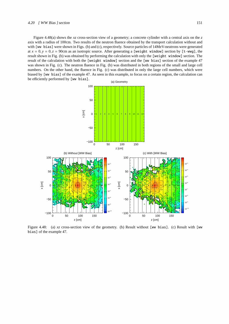
4.20 [ WW Bias ] section 151
Figure4.48(a) shows thexzcross-section view of a geometry; a concrete cylinder with a central axis on thezaxis with a radius of 100cm. Two results of the neutron fluence obtained by the transport calculation without andwith [ww bias]were shown in Figs. (b) and (c), respectively. Source particles of 14MeV-neutrons were generatedat x = 0, y = 0, z = 90cm as an isotropic source. After generating a[weight window] section by[t-wwg], theresult shown in Fig. (b) was obtained by performing the calculation with only the[weight window] section. Theresult of the calculation with both the[weight window] section and the[ww bias] section of the example47was shown in Fig. (c). The neutron fluence in Fig. (b) was distributed in both regions of the small and large cellnumbers. On the other hand, the fluence in Fig. (c) was distributed in only the large cell numbers, which werebiased by[ww bias] of the example47. As seen in this example, to focus on a certain region, the calculation canbe efficiently performed by[ww bias].
File = D:\home\hashimoto\STUDY\houkoku\phits\manual\tex\old-file\WWBG\WWBias\geometry\weight-dose-xz-g.out[t-track] in xyz mesh Date = 13:14 16-Aug-2017
calculated by PHITS 2.95 plotted by ANGEL 4.35
0 50 100 150−100
−50
0
50
100
z [cm]
x [c
m]
(a) Geometry
void
11 2 3 4 5 6 7 8 9 10 11 12
emin = 1.0000E-10 [MeV] emax = 1.0000E+03 [MeV] ymin = -2.0000E+01 [cm] ymax = 2.0000E+01 [cm]
part. = neutron mset = 1
File = D:\home\hashimoto\STUDY\houkoku\phits\manual\tex\old-file\WWBG\WWBias\without-bias\weight-dose-xz-n.out[t-track] in xyz mesh Date = 13:17 16-Aug-2017
calculated by PHITS 2.95 plotted by ANGEL 4.35
0 50 100 150−100
−50
0
50
100
z [cm]
x [c
m]
(b) Without [WW Bias]
1 2 3 4 5 6 7 8 9 10 11 12
10−10
10−9
10−8
10−7
10−6
10−5
10−4
10−3
(µS
v/h)
/(so
urce
/sec
)
emin = 1.0000E-10 [MeV] emax = 1.0000E+03 [MeV] ymin = -2.0000E+01 [cm] ymax = 2.0000E+01 [cm]
part. = neutron mset = 1
File = D:\home\hashimoto\STUDY\houkoku\phits\manual\tex\old-file\WWBG\WWBias\with-bias\weight-dose-xz-n.out[t-track] in xyz mesh Date = 13:17 16-Aug-2017
calculated by PHITS 2.95 plotted by ANGEL 4.35
0 50 100 150−100
−50
0
50
100
z [cm]
x [c
m]
(c) With [WW Bias]
1 2 3 4 5 6 7 8 9 10 11 12
10−10
10−9
10−8
10−7
10−6
10−5
10−4
10−3
(µS
v/h)
/(so
urce
/sec
)
emin = 1.0000E-10 [MeV] emax = 1.0000E+03 [MeV] ymin = -2.0000E+01 [cm] ymax = 2.0000E+01 [cm]
part. = neutron mset = 1
Figure 4.48: (a) xz cross-section view of the geometry. (b) Result without[ww bias]. (c) Result with[wwbias] of the example47.

152 4 SECTIONS FORMAT
4.21 [ Forced Collisions ] section
The forced collisions are used for improving tally statistics or thin target analysis by enlarging the collisionprobabilities. When specified particle comes into a region defined as the forced collision region, the particle isdivided into two particles. One has a weight by (penetration probability)× (its weight), this particle pass throughto the next region. The other has a weight of (1 - penetration probability)× (its weight), and it is forced to collidewith a target in the region. The collision point is randomly determined according to cross sections. Regions andfactors for the forced collisions can be defined in this section. Non-defined regions are set factor zero.
Maximum 6[forced collisions] sections are allowed to be defined in an input file.
[ Forced Collisions ]
part = proton neutron
reg fcl
1 1.000000
11 0.500000
( 2 - 5 8 9 ) 0.200000
( 11 12 15 ) 0.300000
( 6<10[1 0 0]<u=3 ) -0.500000
.... ........
.... ........
You set particle aspart = in the first line. The default ispart = all. part = is the same format as in tallydefinition.
If you want to replace the order of region number (reg) and (fcl), you can set as “fcl reg”. You can usethe skip operatornon. Even if you use GG, you should write the symbol notcell butreg here.
You can use the format( 2 - 5 8 9 ), and you can use the lattice and universe style as( 6 < 10[1 0 0] < u=3 ). But you need to close a value by( ) if it is not a single numeric value. Byusing this format you can set different forced collision factor for each lattice. If the same cell is re-defined, thevalue, which is defined at first, is used.
The forced collision factorfcl means, 0: no forced collision,| f cl| > 1: is an error, and| f cl| ≤ 1 : multiplyforced collision probability byf cl, instead the weight is reduced by 1/ f cl times.
We have two options to control the particle transport and multiple scattering with the weight cut off in theforced collisions region. Whenf cl < 0, secondary particles produced by forced collisions are treated by thenormal process. In this case, weight cut off is not performed. Whenf cl > 0, the forced collision is also appliedto secondary particles. In this case, weight cut off is performed. Even if a particle is killed by this weight cut off,of course the particle is tallied before killed. There is a possibility that all particles are killed by this weight cutoff, if you set the weight cut off and the forced collisions without consideration. For example, it corresponds totallying tracks of secondary particles and information of particles at a distance from the forced collisions region.When you want to transport secondary particles produced by forced collisions, you should decrease the value ofthe cutoff weight parameterwc1(i) in the[parameters] section.

4.22 [ Volume ] section 153
4.22 [ Volume ] section
Volume for GG cell (cm3) can be defined in this section. If the volume is double defined, the value defined inthis[volume] section is used. The volume is utilized in the tally sections. If you do not set volume, it has 1.0 cm3
volume.
[ V o l u m e ]
reg vol
1 1.000000
11 5.000000
( 2 - 5 8 9 ) 2.000000
( 11 12 15 ) 3.000000
16 6.000000
.... ........
.... ........
You can use the format( 2 - 5 8 9 ) for a group. In this case, you need to close a value by( ) ,if it is not a single numeric value.
You cannot use the lattice and universe style as( 6 < 10[1 0 0] < u=3 ). If you want to set cell volumein detail, use the volume definition in the tally section.
If you want to change the order of region number (reg) and volume (vol), you can set as “vol reg”. Youcan use the skip operatornon. Even if you use GG, you should write the symbol notcell butreg here.

154 4 SECTIONS FORMAT
4.23 [ Multiplier ] section
In this section, you can define a multiplier set, which consists of factors depending on energies of particles, tomultiply results of the[t-track] tally. When you use this set, you have to definemultiplier subsections inthe[t-track] section. For example, you can utilize this function for dose estimation using any dose conversionfactor.
In one[multiplier] section, you can define only one multiplier set. The maximum number of the[multiplier]
section defined in an input file is 100. Format of this section is as follows.
[ Multiplier ]
number = -201
interpolation = log
ne = 10
20.0 2.678
30.0 7.020
50.0 18.50
100.0 24.26
200.0 16.13
500.0 10.51
1000.0 10.55
2000.0 10.98
5000.0 12.10
10000.0 12.45
The ID number of the set is determined bynumber, which must be between−299 and−200, and is used in the[t-track] section. You can choose which log-log or lin-lin as the interpolation method of the given data table,by settinginterpolation = log or lin, respectively. The number of the energy point is given byne, and datasets for the point and the factor are defined, respectively, belowne. Note that the data of the energy point shouldbe in ascending order.
When you use the multiplier set defined in this section, you have to usemultiplier option of the[t-track]section. The basic format is given as (C k), whereC is a normalization factor andk is the ID number of the set.It is noted thatk should be negative. Format of themultiplier subsection is given as follows.
multiplier = number of materialpart = neutron
emax = 1000
mat mset1 mset2
1 ( 1 -201 ) ( 2 -202 )
2 ( 1.2 -201 ) ( 3 -202 )
.... .... .... ....
.... .... .... ....
The line ofmultiplier = specifies the number of material where the multiplication is considered. You can useall instead of the number. For this case, one should also useall for mat column below. The second line ofpart= defines the particles considered. The maximum number of the particle is 6 andall can be also used, which isdefault. The multiplication affects only these considered particles. The third line ofemax = defines the maximumenergy of the multiplication. Ifemax is omitted, it is automatically defined as the maximum energy given in the[multiplier] section. The number ofmat column is the material number which is considered to be multiplied.The columns ofmset1, mset2 define the multiplier set. The maximum 6 multiplier can be set. For each set, theresult is printed out. You can define severalmultiplier subsections in one[t-track] section, but you shouldset the number of the multiplier sets to be equal in each subsection.

4.24 [ Mat Name Color ] section 155
4.24 [ Mat Name Color ] section
Material names, size and colors for graphical output by gshow and 3dshow tallies are defined in this section.By default, the name is set as material number and the color is set automatically.
[ Mat Name Color ]
mat name size color
0 void 1 lightgray
1 air 0.5 yellowgreen
2 mat 2 2 orangeyellow
3 mat 3 2 0.067 0.600 1.00 4 - 7 Fe 3 mossgreen
.... ........
.... ........
If you want to replace the order of material number (mat), (name), (size), and (color), set as “mat colorsize name”. You can use the skip operatornon. You must define at least one parameter in “name” and “color”.If no definition, the default values are used.
You can use the format 4 - 7 , but the( 4 - 7 9 10 ) format cannot be used. If you need to useblanks in name definition, the name must be closed by as the example. If you want to use( ), you shouldwrite \( \). In the name, you cannot use . Note that a superscript or subscript in the LaTeX format can beused by writing\ \. For example, in the case of writing\ 208 \Pb, 208Pb is output. The maximum numberof characters of a name that you can define is 80.
When you define two (or more) cells of different densities from each other with the same material number in[cell] section, the cells except the first one are given other material numbers inmatadd=1 (the default setting). Inthis section, you have to set the given numbers, which are outputted in the first part offile(6) (D=phits.out)
as a warning message, in themat column. Even if you setmatadd=0 in [parameters] section, the functionunifying the material number is invalid in this section.
The color definition is based on the format inANGEL . Set color by symbol (r bbb yy), name (red orangeblue), or HSB numericH(hue) S(chroma) B(brightness). In the case HSB numeric definition, close each numericby . If only one HSB numeric is defined, chroma and brightness are set 1.
Color symbols, names, and HSB numerics are shown from next page.
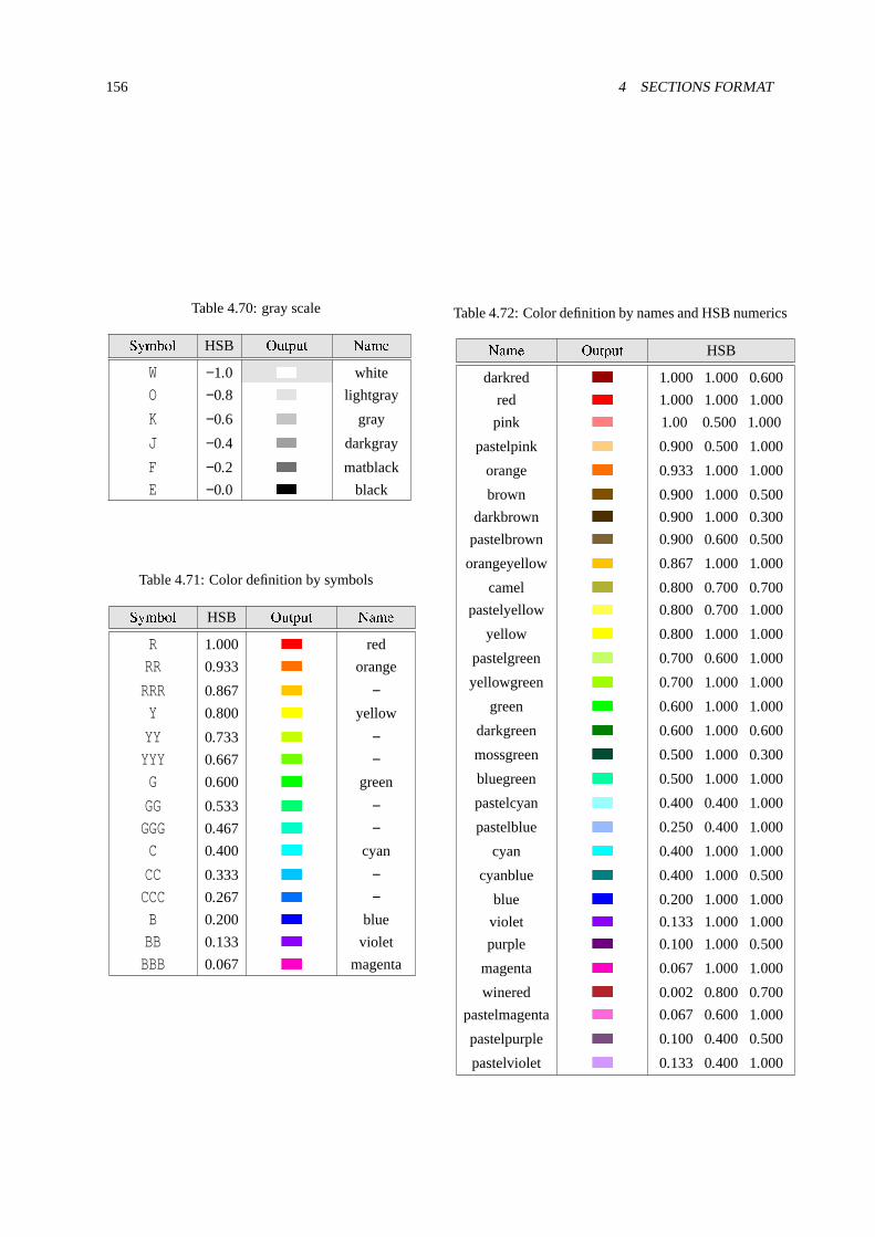
156 4 SECTIONS FORMAT
Table 4.70:gray scale
ÿÿÿÿÿÿ HSB ÿÿÿÿÿÿ ÿÿÿÿ
W −1.0 ÿÿ white
O −0.8 ÿÿ lightgray
K −0.6 ÿÿ gray
J −0.4 ÿÿ darkgray
F −0.2 ÿÿ matblack
E −0.0 ÿÿ black
Table 4.71:Color definition by symbols
ÿÿÿÿÿÿ HSB ÿÿÿÿÿÿ ÿÿÿÿ
R 1.000 ÿÿ red
RR 0.933 ÿÿ orange
RRR 0.867 ÿÿ −Y 0.800 ÿÿ yellow
YY 0.733 ÿÿ −YYY 0.667 ÿÿ −G 0.600 ÿÿ green
GG 0.533 ÿÿ −GGG 0.467 ÿÿ −C 0.400 ÿÿ cyan
CC 0.333 ÿÿ −CCC 0.267 ÿÿ −B 0.200 ÿÿ blue
BB 0.133 ÿÿ violet
BBB 0.067 ÿÿ magenta
Table 4.72:Color definition by names and HSB numerics
ÿÿÿÿ ÿÿÿÿÿÿ HSB
darkred ÿÿ 1.000 1.000 0.600
red ÿÿ 1.000 1.000 1.000
pink ÿÿ 1.00 0.500 1.000
pastelpink ÿÿ 0.900 0.500 1.000
orange ÿÿ 0.933 1.000 1.000
brown ÿÿ 0.900 1.000 0.500
darkbrown ÿÿ 0.900 1.000 0.300
pastelbrown ÿÿ 0.900 0.600 0.500
orangeyellow ÿÿ 0.867 1.000 1.000
camel ÿÿ 0.800 0.700 0.700
pastelyellow ÿÿ 0.800 0.700 1.000
yellow ÿÿ 0.800 1.000 1.000
pastelgreen ÿÿ 0.700 0.600 1.000
yellowgreen ÿÿ 0.700 1.000 1.000
green ÿÿ 0.600 1.000 1.000
darkgreen ÿÿ 0.600 1.000 0.600
mossgreen ÿÿ 0.500 1.000 0.300
bluegreen ÿÿ 0.500 1.000 1.000
pastelcyan ÿÿ 0.400 0.400 1.000
pastelblue ÿÿ 0.250 0.400 1.000
cyan ÿÿ 0.400 1.000 1.000
cyanblue ÿÿ 0.400 1.000 0.500
blue ÿÿ 0.200 1.000 1.000
violet ÿÿ 0.133 1.000 1.000
purple ÿÿ 0.100 1.000 0.500
magenta ÿÿ 0.067 1.000 1.000
winered ÿÿ 0.002 0.800 0.700
pastelmagenta ÿÿ 0.067 0.600 1.000
pastelpurple ÿÿ 0.100 0.400 0.500
pastelviolet ÿÿ 0.133 0.400 1.000

4.25 [ Reg Name ] section 157
4.25 [ Reg Name ] section
Region names and their font sizes for graphic output by[t-gshow], [t-rshow], and[t-3dshow] are definedin this section. When you set the gshow or rshow option in the other tallies, this definition is applied. By default,a region name is set to its region number.
[ Reg Name ]
reg name size
1 cover 1
2 body 0.5
3 cell 2 2
4 cell 3 2
5 - 8 tube 3
.... ........
.... ........
If you want to replace the order of region number (reg), region name (name), and font size (size), set as “regsize name”. You can use the skip operatornon. At least one ofname andsize must be defined. If nothingis defined, it is assumed to be default. You can use the format 4 - 7 , but the( 4 - 7 9 10 ) formatcannot be used. If you need to use blanks in the name definition, the name must be closed by as the example.If you want to use( and), you should write\( and\), respectively. Brackets and cannot be used in the namedefinition. Note that a superscript or subscript in the LaTeX format can be used by writing\ \. For example,in the case of writing \ 208 \Pb, 208Pb is output. The maximum number of characters of a name that you candefine is 80. You can specify a font size as a relative value to the default size.
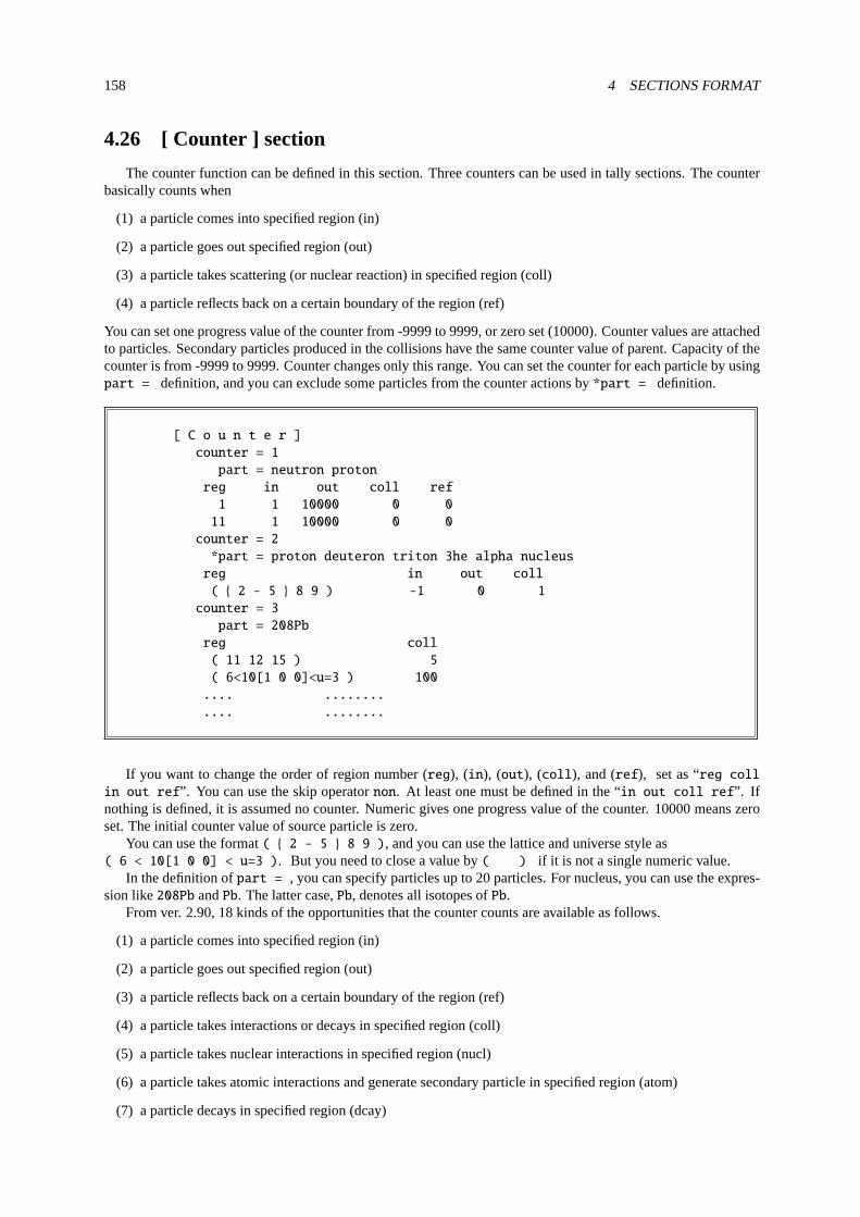
158 4 SECTIONS FORMAT
4.26 [ Counter ] section
The counter function can be defined in this section. Three counters can be used in tally sections. The counterbasically counts when
(1) a particle comes into specified region (in)
(2) a particle goes out specified region (out)
(3) a particle takes scattering (or nuclear reaction) in specified region (coll)
(4) a particle reflects back on a certain boundary of the region (ref)
You can set one progress value of the counter from -9999 to 9999, or zero set (10000). Counter values are attachedto particles. Secondary particles produced in the collisions have the same counter value of parent. Capacity of thecounter is from -9999 to 9999. Counter changes only this range. You can set the counter for each particle by usingpart = definition, and you can exclude some particles from the counter actions by*part = definition.
[ C o u n t e r ]
counter = 1
part = neutron proton
reg in out coll ref
1 1 10000 0 0
11 1 10000 0 0
counter = 2
*part = proton deuteron triton 3he alpha nucleus
reg in out coll
( 2 - 5 8 9 ) -1 0 1
counter = 3
part = 208Pb
reg coll
( 11 12 15 ) 5
( 6<10[1 0 0]<u=3 ) 100
.... ........
.... ........
If you want to change the order of region number (reg), (in), (out), (coll), and (ref), set as “reg collin out ref”. You can use the skip operatornon. At least one must be defined in the “in out coll ref”. Ifnothing is defined, it is assumed no counter. Numeric gives one progress value of the counter. 10000 means zeroset. The initial counter value of source particle is zero.
You can use the format( 2 - 5 8 9 ), and you can use the lattice and universe style as( 6 < 10[1 0 0] < u=3 ). But you need to close a value by( ) if it is not a single numeric value.
In the definition ofpart = , you can specify particles up to 20 particles. For nucleus, you can use the expres-sion like208Pb andPb. The latter case,Pb, denotes all isotopes ofPb.
From ver. 2.90, 18 kinds of the opportunities that the counter counts are available as follows.
(1) a particle comes into specified region (in)
(2) a particle goes out specified region (out)
(3) a particle reflects back on a certain boundary of the region (ref)
(4) a particle takes interactions or decays in specified region (coll)
(5) a particle takes nuclear interactions in specified region (nucl)
(6) a particle takes atomic interactions and generate secondary particle in specified region (atom)
(7) a particle decays in specified region (dcay)

4.26 [ Counter ] section 159
(8) a particle takes elastic scattering in specified region (elst)
(9) a particle takes inelastic scattering in specified region (iels)
(10) a particle takes fission in specified region (fiss)
(11) a particle generates delta-rays in specified region (delt)
(12) a particle generates atomic fluorescence x-rays in specified region (fluo)
(13) a particle generates Auger electrons in specified region (auge)
(14) a particle takes bremsstrahlung in specified region (brem)
(15) a particle takes photoelectric effect in specified region (phel)
(16) a particle takes Compton scattering in specified region (cmpt)
(17) a particle generates electron-positron pair in specified region (pprd)
(18) a particle is annihilated in specified region (anih)
Here, nucl, atom, and dcay, which are particular interactions, belong to coll. elst, iels, and fiss, which are nuclearreactions, belong to nucl. delt, fluo, auge, brem, phel, cmpt, pprd, and anih, which are atomic interactions, belongto atom. When you want to analyze the PHITS simulation in detail, set these keywords. Note that if you set colland nucl at the same time, the counting is duplicated when a nuclear reaction event occurs.
If you set (fiss), the counter is called when fission channels of the nuclear data library and the statistical decaymodel (GEM) are chosen.

160 4 SECTIONS FORMAT
4.27 [ Timer ] section
The timer function can be defined in this section. The timer controls the time of each particle when (1) aparticle comes into specified region, (2) a particle goes out specified region, (3) a particle takes scattering inspecified region, and (4) a particle reflects back on a certain boundary of the region. You can set the time to bezero(-1), stopped(1) or nothing(0).
[ T i m e r ]
reg in out coll ref
1 0 -1 0 0
11 1 0 0 0
.... .... .... .... ....
.... .... .... .... ....
.... .... .... .... ....
If you want to replace the order of region number (reg), (in), (out), (coll), and (ref), set as “reg coll inout ref”. You can use the skip operatornon. At least one must be defined in the “in out coll ref”. Ifnothing is defined, it is assumed no action.
You can use the format( 2 - 5 8 9 ), and you can use the lattice and universe style as( 6 < 10[1 0 0] < u=3 ). But you need to close a value by( ) if it is not a single numeric value.
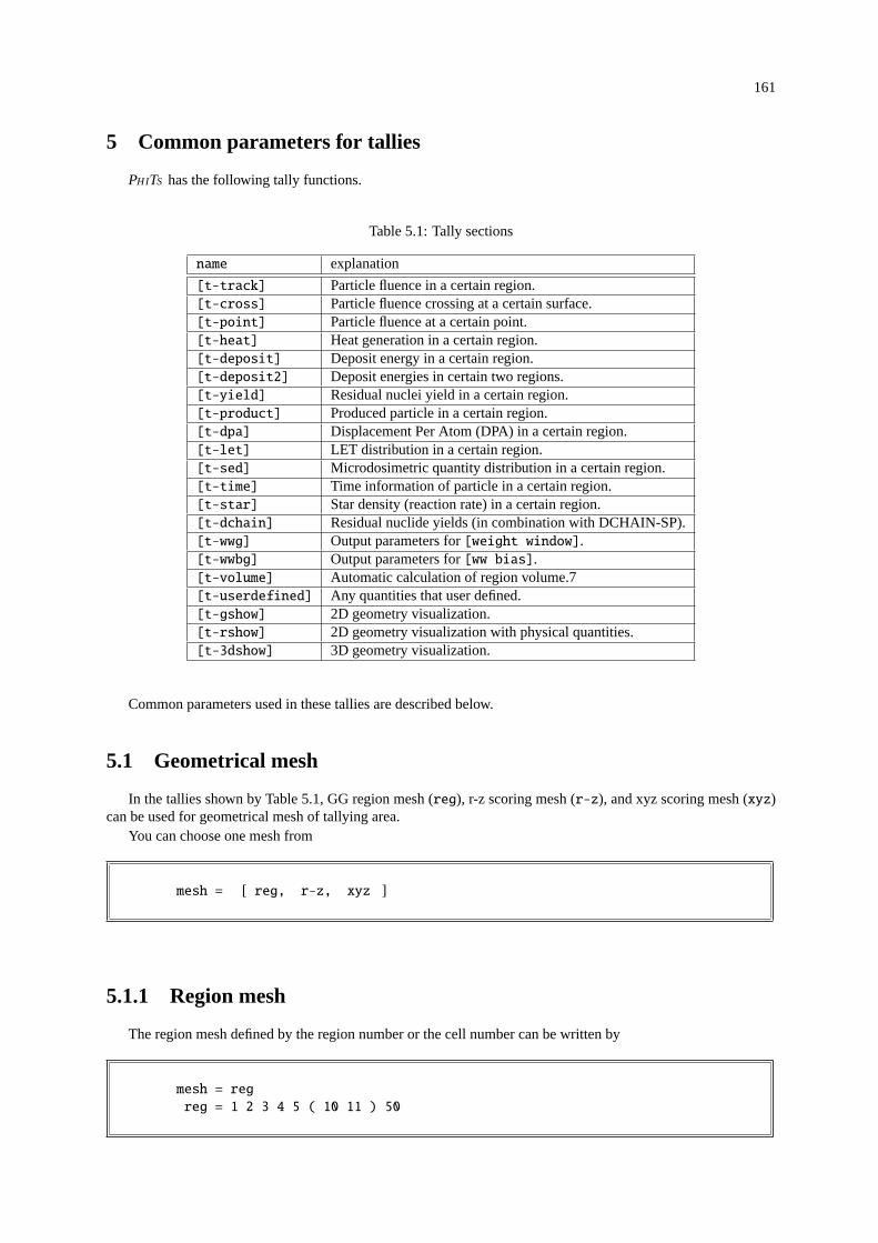
161
5 Common parameters for tallies
PHITS has the following tally functions.
Table 5.1:Tally sections
name explanation
[t-track] Particle fluence in a certain region.[t-cross] Particle fluence crossing at a certain surface.[t-point] Particle fluence at a certain point.[t-heat] Heat generation in a certain region.[t-deposit] Deposit energy in a certain region.[t-deposit2] Deposit energies in certain two regions.[t-yield] Residual nuclei yield in a certain region.[t-product] Produced particle in a certain region.[t-dpa] Displacement Per Atom (DPA) in a certain region.[t-let] LET distribution in a certain region.[t-sed] Microdosimetric quantity distribution in a certain region.[t-time] Time information of particle in a certain region.[t-star] Star density (reaction rate) in a certain region.[t-dchain] Residual nuclide yields (in combination with DCHAIN-SP).[t-wwg] Output parameters for[weight window].[t-wwbg] Output parameters for[ww bias].[t-volume] Automatic calculation of region volume.7[t-userdefined] Any quantities that user defined.[t-gshow] 2D geometry visualization.[t-rshow] 2D geometry visualization with physical quantities.[t-3dshow] 3D geometry visualization.
Common parameters used in these tallies are described below.
5.1 Geometrical mesh
In the tallies shown by Table5.1, GG region mesh (reg), r-z scoring mesh (r-z), and xyz scoring mesh (xyz)can be used for geometrical mesh of tallying area.
You can choose one mesh from
mesh = [ reg, r-z, xyz ]
5.1.1 Region mesh
The region mesh defined by the region number or the cell number can be written by
mesh = reg
reg = 1 2 3 4 5 ( 10 11 ) 50

162 5 COMMON PARAMETERS FOR TALLIES
each region number or cell number is separated by blank. If you want to combine some regions, use( ). Thefollowing format can be used for defining sequential region numbers.
mesh = reg
reg = 1 - 5 ( 10 11 ) ( 6 < 10[1 0 0] < u=3 )
In the formatn1 - n2 (n1 is smaller than n2), you can specify regions fromn1 to n2. You can’t specify like( n1 - n2 ). Styles( ) and( all ) can be used, but ( ) cannot be used. You can usethe lattice and universe style as( 6 < 10[1 0 0] < u=3 ). By using above format, you can tally from eachlattice individually. And if you set region asreg = all, all regions become tallying region. However, cells whichdo not belong to bottom level, are not included.
5.1.2 Definition of the region and volume for repeated structures and lat-tices
When you define regions including repeated structures and lattices, you must close your definition by( ).A level structure is indicated by<. In the case an intermediate level has the lattice structure, you can specifylattices using[ ] represented by the lattice coordinate (s, t,u), after the cell number as160[1:2 3:6 1:1].In this example, lattices, which from 1 to 2 ins direction, 3 to 6 int direction, and 1 inu direction, are defined.Or you can specify individually as160[1 3 4, 2 3 4, 3 3 4]. The style( ) in one level can be used tocombine some regions. See next example.
Example 48:mesh = reg example (1)
1: mesh = reg
2: reg = (all)
3: ( 201 - 205 )4: ( 161 < 160[1:2 3:6 1:1] )
5: ( (201 202 203 204) < (161 162 163 ) )
6: ( ( 90 100 ) 120 < 61 ( 62 63 ) )
This region mesh definition is echoed as
Example 49:mesh = reg example (2)
1: mesh = reg # mesh type is region-wise
2: reg = ( all ) ( 201 - 205 ) ( 161 < 160[ 1:2 3:6 1:1 ] ) ( (3: 201 - 204 ) < ( 161 - 163 ) ) ( ( 90 100 ) 120 < 614: ( 62 63 ) )
5: volume # combined, lattice or level structure
6: non reg vol # reg definition
7: 1 10001 8.1000E+01 # ( all )
8: 2 10002 5.0000E+00 # ( 201 - 205 )9: 3 10003 1.0000E+00 # ( 161 < 160[ 1 3 1 ] )
10: 4 10004 1.0000E+00 # ( 161 < 160[ 2 3 1 ] )
11: 5 10005 1.0000E+00 # ( 161 < 160[ 1 4 1 ] )
12: 6 10006 1.0000E+00 # ( 161 < 160[ 2 4 1 ] )
13: 7 10007 1.0000E+00 # ( 161 < 160[ 1 5 1 ] )
14: 8 10008 1.0000E+00 # ( 161 < 160[ 2 5 1 ] )
15: 9 10009 1.0000E+00 # ( 161 < 160[ 1 6 1 ] )
16: 10 10010 1.0000E+00 # ( 161 < 160[ 2 6 1 ] )
17: 11 10011 4.0000E+00 # ( ( 201 - 204 ) < ( 161 - 163 ) )18: 12 10012 2.0000E+00 # ( ( 90 100 ) < 61 )
19: 13 10013 1.0000E+00 # ( 120 < 61 )
20: 14 10014 2.0000E+00 # ( ( 90 100 ) < ( 62 63 ) )
21: 15 10015 1.0000E+00 # ( 120 < ( 62 63 ) )

5.1 Geometrical mesh 163
In the input, it looks only 5 regions defined, but in the input echo, you can see 15 regions are defined for tally. Inthis input echo, region numbers are defined automatically starting from 10001, and the volume of each cell is set 1because of no [volume] definition.
We explain the detail of 15 regions appears in the volume description of this input echo.First for( all ), 81 cells are defined in the bottom level, so the volume of( all ) is set 81. If the volume
of the cell is defined correctly in the[volume] section, you don’t need to define the volume here again.Next for( 201 - 205 ), this combined region has volume 5 in the echo, since this combined regions have
5 cells of bottom level. This is also not required to re-define here if the volume is set in the[volume] section.For( 161 < 160[1:2 3:6 1:1] ), the region 161 is included as a lattice in region 160. In this expression
in the lattice coordinate system, 8 lattices of the region 160 from 1 to 2 insdirection, 3 to 6 int direction, and 1 inu direction, are used for the tally. In the echo, the number of regions in bottom level is echoed 1. In the case, youhave to specify the volume by yourself by the volume definition below.
For( (201 202 203 204) < (161 162 163 ) ), some regions are defined in each level, but these are allclosed by( ), so it means one region as a whole. In this case, given volume by the echo is not correct, so setvolume manually by the volume definition below.
For ( ( 90 100 ) 120 < 61 ( 62 63 ) ), there are two independent regions in each level, so 4 regionsare defined here. In this case given volume by the echo is not correct too, so set volume manually in the[volume]
section.You can set volume as below.
mesh = reg
reg = 1 2 3 4 ( 5 < 12 ) ( 13 - 17 )volume
reg vol
1 1.0000
2 5.0000
3 6.0000
4 1.0000
10001 6.0000
10002 5.0000
In above example, region numbers from 1 to 4 are set normally as you can see, but regions( 5 < 12 ) and(13 - 17 ) have numbers 10001 and 10002. These big values are given in an input echo automatically. You cansee and paste this settings from the input echo.
If you want to change the order of region number (reg) and volume (vol), set as “vol reg”. You can use theskip operatornon.
In the input echo, numbered entry is given innon column. Whenaxis = reg, the numbered entry is used asa value of X axis. Even if you use GG, use the symbol notcell butreg here.
When you define regions in the bottom level, set same region twice as( 3000 < 3000[1:2 3:61:1] ).
5.1.3 r-z mesh
When you use the r-z scoring mesh, first, offsets for x and y coordinate of the center of cylinder can be definedas
mesh = r-z
x0 = 1.0
y0 = 2.0
This can be omissible. Then, define r and z mesh as

164 5 COMMON PARAMETERS FOR TALLIES
mesh = r-z
r-type = [1-5]
..........
..........
z-type = [1-5]
..........
..........
Mesh definition is described later.You can addθ degree of freedom in r-z mesh of[t-track] tally. You can usea-type mesh definition to
specifyθ of r-z mesh in the same manner as in the other angle mesh cases. However, the maximum angle ofθmesh is restricted 360 degree (2π) in this case. You can obtain theθ dependence of results of[t-track] tally bysettingaxis=rad or axis=deg. Therad represents theθ in radian, whiledeg in degree.
5.1.4 xyz mesh
When you use the xyz scoring mesh, set x, y, and z mesh as
mesh = xyz
x-type = [1-5]
..........
..........
y-type = [1-5]
..........
..........
z-type = [1-5]
..........
..........
Mesh definition is described later.
5.2 Energy mesh
Energy mesh begins as
e-type = [1-5]
..........
..........
”e1-type” and ”e2-type” are also used in DEPOSIT2 tally. Mesh definition is described later.
5.3 LET mesh
LET mesh begins as

5.4 Time mesh 165
l-type = [1-5]
..........
..........
Mesh definition is described later.
5.4 Time mesh
Time mesh is defined as
t-type = [1-5]
..........
..........
Mesh definition is described later.
5.5 Angle mesh
Angle mesh in cross tally is defined as
a-type = [1, 2, -1, -2]
..........
..........
If a-type is defined by positive number, this mesh denotes cosine mesh. Ifa-type is defined by negativenumber, the mesh denotes angle mesh. Mesh definition is described later.
5.6 Mesh definition
There are 8 kinds of mesh definition ase-type, t-type, x-type, y-type, z-type, r-type, a-typeandl-type. The format is common for every mesh types. So only thee-type definition is described below. Forother types, replace “e” into “t”, “x”, “y”, ... and “a”. For example, replace “ne” as “nt, nx, ny, ... , na”,“emin” as “tmin, xmin, ymin, ... , amin”, and so on.
5.6.1 Mesh type
You can use 5 kinds of mesh type as shown below.It is noted that you can use only 1, 2 (-1, -2) mesh types ina-type definition. Each mesh type format is shown
in followings.
5.6.2 e-type= 1
When you usee-type=1, set number of group, then numerical data as

166 5 COMMON PARAMETERS FOR TALLIES
Table 5.2:mesh type
mesh type explanation
1 give number of groups and mesh points by data2 give number of groups, minimum and maximum values.
mesh is divided equally by linear scale.3 give number of groups, minimum and maximum values.
mesh is divided equally by log scale.4 give mesh width, minimum and maximum values.
mesh points are given by linear scale.Number of groups is set automatically as resulting maximumvalue becomes same with given value, or takes larger value withsmall excess as possible.
5 give minimum and maximum values and log value of mesh widthmesh points are given by log scale.Number of groups is set automatically as resulting maximumvalue becomes same with given value, or takes larger value withsmall excess as possible.
e-type = 1
ne = number of groupdata(1) data(2) data(3) data(4)data(5) data(6) data(7) data(8).........
.........
data(ne+1)
You can use multi lines without any symbols for line connection.

5.7 Other tally definitions 167
5.6.3 e-type= 2, 3
When you usee-type = 2, 3, set number of group, minimum value, and maximum value as
e-type = 2, 3
ne = number of groupemin = minimum valueemax = maximum value
5.6.4 e-type= 4
When you usee-type=4, set mesh width, minimum value, and maximum value as
e-type = 4
edel = width of meshemin = minimum valueemax = maximum value
5.6.5 e-type= 5
When you usee-type= 5, set mesh width, minimum value, and maximum value as
e-type = 5
edel = log( width of mesh)emin = minimum valueemax = maximum value
In the case, mesh width is for log scale, i.e., edel= log( Mi+1 / M i ).
5.7 Other tally definitions
5.7.1 Particle definition
You can define particles as
part = proton neutron pion+ 3112 208Pb
or
168 5 COMMON PARAMETERS FOR TALLIES
part = proton
part = neutron
part = pion+
part = 3112
part = 208Pb
See Table3.4for particle identification. You can also use the kf code number.
If you define all particles as
part = all
Maximum 6 particles can be define in a tally. If you want to tally more particles, use another tally sections ofthe same kind of tally.
If you want to tally some particles as a group, you can use( ) as the following. The maximum number insidethe( ) is 6.
part = ( proton neutron ) all pion+ 3112 208Pb
In this case, as the first group, the sum of proton and neutron contribution is tallied, the second is the sum of all. 5groups of the particle are printed out in this tally.
For nucleus, you can use the expression like208Pb andPb. The later case,Pb, denotes all isotopes ofPb.
5.7.2 axis definition
X axis value for output is described here. There are many kinds ofaxis shown as (depend on kinds of talliesor geometrical meshes),
eng, reg, x, y, z, r, t, xy, yz, zx, rz,
cos, the, mass, charge, chart, dchain
let, t-eng, eng-t, t-e1, e1-t, t-e2, e2-t, e12, e21
axis = eng
You can set multipleaxis per one tally by
axis = eng x y
or,

5.7 Other tally definitions 169
axis = eng
axis = x
axis = y
If you define multiple axes, output results are written in different files. So you need to specify multiple output filesas shown in the next subsection when multiple axes are defined.
It should be noted that you can define only oneaxis in a [t-yield] section from ver. 2.50. This restrictionwas implemented to calculate statistical uncertainties correctly. If you want to define several axes in the[t-yield]
tally, you have to set the corresponding number of[t-yield] sections in a input file.
5.7.3 file definition
The format to define name of output file is,
file = file.001 file.002 file.003
Note that the file name should not have the extension of “.eps”or “.vtk”. As described before, when you set multipleaxis, set output files for each axis like following example.
file = file.001
file = file.002
file = file.003
5.7.4 resfile definition
The format to specify a file name of past tally in the restart calculation is,
resfile = file.001
where the file name must be written with full pathname. Even if severalresfile parameters are set in a tallysection, only the earliest one is used.resfile is set tofile by default. In this case, results of the past tally areoverwritten.
5.7.5 unit definition
Set output unit as
unit = number
The unit number and its meanings are described in each tally explanation.
170 5 COMMON PARAMETERS FOR TALLIES
5.7.6 factor definition
You can set normalize factor by this format.
factor = number
This value is multiplied to output values. When you use the [t-gshow] tally, this factor defines line thicknessinstead.
5.7.7 output definition
Set output type as
output = name of output
Details are described in each tally explanation.
5.7.8 info definition
This option defines whether detailed information is output or not. Set 0 or 1 as
info = 0, 1
5.7.9 title definition
This option is for title as
title = title of the tally
It is omissible, and in this case, default is used.
5.7.10 ANGEL parameter definition
In order to add ANGEL parameters in tally output, define as
angel = xmin(1.0) ymin(1.3e-8)
Defined parameters are converted to the ANGEL format as
p: xmin(1.0) ymin(1.3e-8)

5.7 Other tally definitions 171
These parameters change the minimum of the horizontal and vertical axes, respectively. The main ANGEL param-eters are shown in Table5.3. Please see the ANGEL manual in more detail.
Table 5.3:ANGEL parameter
ANGEL parameter Explanation
xmin Minimum of horizontal axis.xmax Maximum of horizontal axis.ymin Minimum of vertical axis.ymax Maximum of vertical axis.xlin Change horizontal axis to liner scale.xlog Change horizontal axis to logarithmic scale.ylin Change vertical axis to liner scale.ylog Change vertical axis to logarithmic scale.cmnm Convert cm to nm.cmum Convert cm toµm.cmmm Convert cm to mm.cmmt Convert cm to m.cmkm Convert cm to km.
From ver. 2.89, the default size was changed from A4 to US letter. ANGEL parameters,a4us(US letter),a3pp(A3), a4pp(A4), a5pp(A5), b3pp(B3), b4pp(B4), andb5pp(B5) can be used to change an output size of aneps file. The characters given in parentheses represent each output size.
5.7.11 SANGEL parameter definition
This definition can be used to insert all ANGEL parameters into tally output files unlike the usual ANGELparameter definition, which can specify only ANGEL parameters defined byp:. For example, defininginfl:parameter for ANGEL, the tally file includes an experimental data file, and both calculated results and the experi-mental data can be plotted in a figure (eps file).
The SANGEL parameter can be set using the formatsangel=number of definition lines, and then writing thelines to define the ANGEL parameters. An example withsangel is as follows.
sangel = 2
infl:exp.dat
w: ($\theta=$ 0 deg) / X(10) Y(100)
whereexp.dat is a data file of the experimental data. The data can be shown on the figure of the tally result. Byusingw: parameter, the comment “θ=0 deg” can be put at the coordinate ofX=10, Y=100 in the figure.
5.7.12 2d-type definition
When you define 2 dimensional output asaxis = xy, you must set this2d-type option as
2d-type = 1, 2, 3, 4, 5, 6, 7
These 2d-types give the format of data arrange.
• 2d-type = 1, 2, 3, 6, 7Data are written by below format (the example is written by Fortran style).
( ( data(ix,iy), ix = 1, nx ), iy = ny, 1, -1 )

172 5 COMMON PARAMETERS FOR TALLIES
10 data are written in a line. Also a header for the ANGEL input is inserted. The ANGEL header is insertedby 2d-type = 1 for contour plot,2d-type = 2 for cluster plot,2d-type = 3 for color plot,2d-type =6 for cluster and contour plot,2d-type = 7 for color and contour plot.
• 2d-type = 4Data are written by below format
do iy = ny, 1, -1
do ix = 1, nx
( x(ix), y(iy), data(ix,iy) )
end do
end do
3 data ofx(ix), y(iy) anddata(ix,iy) are written in a line.
• 2d-type = 5Data are written by below format
y/x ( x(ix), ix = 1, nx )
do iy = ny, 1, -1
( y(iy), data(ix,iy), ix = 1, nx )
end do
nx + 1 data are written in a line, and totalny + 1 lines. It is useful to use in the tabular soft like Excel.
5.7.13 gshow definition
This option can be used in all tallies without [t-gshow] and [t-rshow]. If you set gshow option with xyz mesh,xy, yz, or xz axis, and 2d-type= 1, 2, or 3, ANGEL can create a graphical plot with region boundary and materialname, or region name, or lattice number on the two dimensional output. You can also obtain graphical plotsdirectory from thePHITS calculation by the “epsout” option.
gshow = 0, 1, 2, 3, 4
In above example, 0 means no gshow option, 1 means gshow with region boundary, 2 means gshow with regionboundary and material name, 3 means gshow with region boundary and region name, 4 means gshow with regionboundary and lattice numbers. When you increase the resolution of the plot byresol parameter, the indicationof region name, material name and lattice number on the graph are sometimes disturbed. In this case, you shouldincrease the mesh points instead ofresol.
You can see your geometry plot on a graph without transport calculation by settingicntl = 8 in the[parameters]section, and this gshow option. You should check whether regions are correct, and a xyz mesh resolution is goodor not, before long time calculation.
5.7.14 rshow definition
You can usershow definition in all tallies except for[t-cross] and[t-gshow] tallies. This option is avail-able with region mesh, xy, yz, zx axis. This option makes a two dimensional plot in which each region is coloredwith the amount of its region’s output value. And region boundaries, material name, or region name numbers arealso displayed. The xyz mesh definition is required after thisrshow definition.

5.7 Other tally definitions 173
rshow = 1, 2, 3
x-type = [2,4]
..........
..........
y-type = [2,4]
..........
..........
z-type = [2,4]
..........
..........
rshow = 0means no rshow option, 1 means rshow with region boundary, 2 means rshow with region boundaryand material name, 3 means rshow with region boundary and region name numbers. Ifrshow =0, xyz meshdefinition is not required, comment out it. When you increase the resolution of the plot byresol parameter, theindication of region name, material name and lattice number on the graph are sometimes disturbed. In this case,you should increase the mesh points instead ofresol.
If you use the rshow option with “reg” mesh, there is no output for the values of each region. In this case, youcannot re-plot the figure because of no original data. When thisrshow option is used, usuallyaxis is set as xy,yz, and zx. But you should use in additionaxis = reg in order to save results into another file, for re-plotting.You can re-plot figures from saved data and [t-rshow] tally function.
You can execute this option without transport calculation by usingicntl =10 in the[parameters] section.Foricntl =10, PHITS makes a two dimensional plot for the tallies with reg mesh, xy, yz, zx axis and rshow= 1,2, 3. In the figure, different colors are used for different materials. You should check whether regions are correctand a xyz mesh resolution is good or not, before long time calculation.
5.7.15 x-txt, y-txt, z-txt definition
If you want to change x, y, and z axis titles in the output figure, use these option. These title cannot be definedin the ANGEL parameter.
x-txt = x axis title
y-txt = y axis title
z-txt = z axis title
5.7.16 volmat definition
The volmat parameter corrects a volume where xyz mesh crosses region boundaries. This option is effectivein the case that mesh is xyz, and the material parameter is defined. This corrected volume is calculated by theMonte Carlo method for specified material.volmat denotes the number of scanning parallel to x, y, and z axisrespectively for the Monte Carlo calculation. So if you set too large volmat, the calculation takes long time. Youneed to take care of it. If volmat is given by negative value, all xyz mesh is scanned. If positive value, the scanningis not performed when 8 apexes of the mesh are included in the same material.
5.7.17 epsout definition
If you setepsout =1, output file is treated by ANGEL automatically and an eps file is created. This eps filename is named by replacing the extension into “.eps”. Withitall = 1 setting, the eps file is created after everybatch calculation. You can monitor thePHITS results in real time, by displaying the eps file with the ghostview andby setting refresh function for a file updating by typing “w” key on the ghostview.
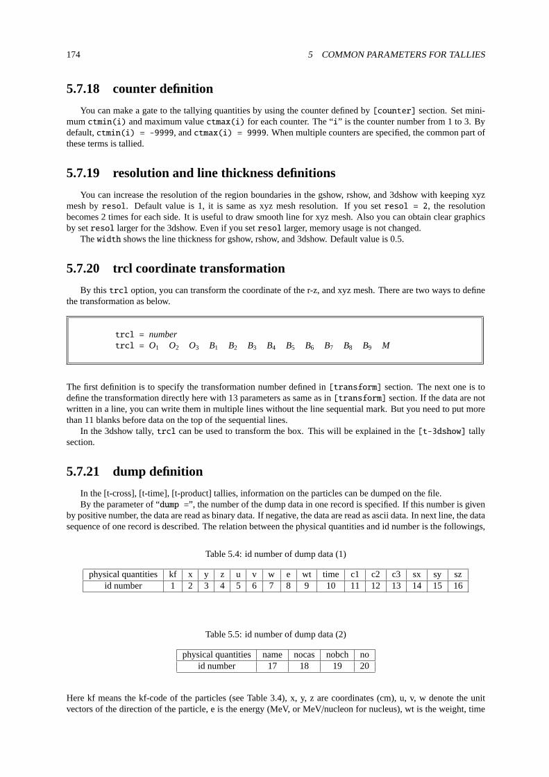
174 5 COMMON PARAMETERS FOR TALLIES
5.7.18 counter definition
You can make a gate to the tallying quantities by using the counter defined by[counter] section. Set mini-mumctmin(i) and maximum valuectmax(i) for each counter. The “i” is the counter number from 1 to 3. Bydefault,ctmin(i) = -9999, andctmax(i) = 9999. When multiple counters are specified, the common part ofthese terms is tallied.
5.7.19 resolution and line thickness definitions
You can increase the resolution of the region boundaries in the gshow, rshow, and 3dshow with keeping xyzmesh byresol. Default value is 1, it is same as xyz mesh resolution. If you setresol = 2, the resolutionbecomes 2 times for each side. It is useful to draw smooth line for xyz mesh. Also you can obtain clear graphicsby setresol larger for the 3dshow. Even if you setresol larger, memory usage is not changed.
Thewidth shows the line thickness for gshow, rshow, and 3dshow. Default value is 0.5.
5.7.20 trcl coordinate transformation
By thistrcl option, you can transform the coordinate of the r-z, and xyz mesh. There are two ways to definethe transformation as below.
trcl = numbertrcl = O1 O2 O3 B1 B2 B3 B4 B5 B6 B7 B8 B9 M
The first definition is to specify the transformation number defined in[transform] section. The next one is todefine the transformation directly here with 13 parameters as same as in[transform] section. If the data are notwritten in a line, you can write them in multiple lines without the line sequential mark. But you need to put morethan 11 blanks before data on the top of the sequential lines.
In the 3dshow tally,trcl can be used to transform the box. This will be explained in the[t-3dshow] tallysection.
5.7.21 dump definition
In the [t-cross], [t-time], [t-product] tallies, information on the particles can be dumped on the file.By the parameter of “dump =”, the number of the dump data in one record is specified. If this number is given
by positive number, the data are read as binary data. If negative, the data are read as ascii data. In next line, the datasequence of one record is described. The relation between the physical quantities and id number is the followings,
Table 5.4:id number of dump data (1)
physical quantities kf x y z u v w e wt time c1 c2 c3 sx sy szid number 1 2 3 4 5 6 7 8 9 10 11 12 13 14 15 16
Table 5.5:id number of dump data (2)
physical quantities name nocas nobch noid number 17 18 19 20
Here kf means the kf-code of the particles (see Table3.4), x, y, z are coordinates (cm), u, v, w denote the unitvectors of the direction of the particle, e is the energy (MeV, or MeV/nucleon for nucleus), wt is the weight, time
5.7 Other tally definitions 175
is the initial time (ns), c1, c2, c3 are the values of counters, and sx, sy, sz are the unit vectors of the directionof spin, respectively. name is a collision number of the particle, nocas is a current history number of this batch,nobch is a current batch number, no is a cascade id in this history. These are assumed as real*8 for the binary data,n(1p1e24.15) data format for the ascii data.
For an example, one record has 9 data as
kf e wt x y z u v w
To read this data, we write the parameters as
dump = 9
1 8 9 2 3 4 5 6 7
When you use this dump parameter,axis andfile are restricted to one axis and one file, andunit is always1. The dumped data are written on a file named “***dmp”, where “***”indicates the file name specified by“file=***”. The normal output of the tally is written on “***”. From this file, you can get the information onthe total normalization factor. (In the former version of PHITS (before 2.66), the normal output was written ona configuration file (.cfg), and the dumped data were written on “***”.) In the parallel computing, files to thenumber of (PE−1) corresponding to each PE (Processor Element) are created for writing and reading dumped data.If you setidpara=0 or 1, a file is made in the directory named by/wk/uname/ on each of the nodes. If you setidpara=1 or 3, the each IP number is put at the end of the filename. The each PE writes down its result on onlythe corresponding file, and reads it from the same file in the re-calculation.

176 5 COMMON PARAMETERS FOR TALLIES
5.8 Function to sum up two (or more) tally results
After version 2.74, PHITS has a function to sum up two (or more) tally results. There are two methods forsum up; one is to integrate the tally results considering the history number of each simulation, while the other isto add the tally results weighted by user defined ratios. The former can be used for the parallel calculation oncomputers in which MPI protocol is not installed. On the other hand, the latter is suit for the simulation withdifferent source terms whose intensities cannot be fixed before the simulation, such as that for Intensity-ModulatedRadiation Therapy (IMRT).
In order to use this function, you have to satisfy the following conditions:
• icntl is set to 13 in [parameters] section
• The parameters for each tally results such asmesh, axis andpart are identical to one another
• “sumtally” subsection is defined in the tally section that outputs one of the summing up tallies.43 44
“sumtally” subsection is ignored whenicntl parameter is not set to 13 in [parameters] section. (From ver. 2.88,“sumtally” works all tallies.) Please see ppt file or sample input file in\phits\utility\sumtally in detail.
“sumtally” subsection should be defined between the lines ofsumtally start andsumtally end writtenin the tally section that outputs one of the summing up tallies. Theset definition is ignored in the sumtallysubsection.
The parameters used in “sumtally” subsection are summarized in Table5.6.
Table 5.6:Parameters used in “sumtally” subsection
name value description
isumtally = 1(default), 2 Summing up procedure
1: Integration of tally results
considering history number of each simulation
2: Sum of tally results weighted by user
defined ratios
nfile = Number Number of summing up files
(next line) filename value Summing up file name, weighted value
Sum of the weighted values is automatically
normalized to sumfactor for isumtally=2
sfile = filename Output file name
sumfactor = (Omissible, D=1.0) Normalization factor
For example, if you have two tally results “result-1.out” and “result-2.out” that were obtained frommaxcas
= 100 andmaxbch = 10 and 20, respectively, and you would like to obtain their summing up results consideringtheir histories, you have to write:
Example 50: example forisumtally=1
1: sumtally start
2: isumtally = 1 $(D=1) sumtally option, 1:integration, 2:weighted sum
3: nfile = 2 $ number of tally files
4: result-1.out 1.0
5: result-2.out 1.0
6: sfile = result-s.out $ file name of output by sumtally option
7: sumfactor = 1.0 $ (D=1.0) normalization factor
8: sumtally end
Using this sumtally subsection, you can obtain the results formaxcas = 100 andmaxbch = 30. Please besure that the initial random seeds for calculating “result-1.out” and “result-2.out” should be different from each
43 Before ver. 2.81, this function is available even iffile parameter is not defined in the tally section. However, after ver. 2.82, PHITSoccurs the error in the setting without the definition offile.
44 Before ver. 2.85, only one “sumtally” subsection can be defined in a PHITS input file.

5.8 Function to sum up two (or more) tally results 177
other, otherwise you would get biased results for certain random numbers. The most recommended method forchanging the initial random seed is to useirskip parameter. The weighted value for each tally outputs aregenerally set to 1 forisumtally = 1, unless you would like to change the weight of source particles. The outputfile obtained from this sumtally section, “result-s.out”, can be used for restart calculation by settingistdev < 0.Note that the initial random seed in the last file of the summing up files is used.
Forisumtally = 2, the weighted summation of the tally results,X, is calculated by the following equation:
X = FN∑
j=1
r j
rX j (19)
whereF is the normalization factor defined bysumfactor, N is the number of summing up files defined bynfile, X j is the j-th tally results,r j is the weighted value ofj-th tally, andr is the sum ofr j , i.e. r =
∑Nj=1 r j . The
uncertainty of the summation value,σX, can be calculated by
σX = F
√√√ N∑j=1
( r j
r
)2σ2
X j(20)
whereσX j is the standard deviation ofj-th tally results.If you have two tally results “result-l.out” and “result-r.out”, and you would like to sum up them weighted by
factors of 2.0 and 3.0, respectively, you have to write:
Example 51: example forisumtally=2
1: sumtally start
2: isumtally = 2 $(D=1) sumtally option, 1:integration, 2:weighted sum
3: nfile = 2 $ number of tally files
4: result-l.out 2.0
5: result-r.out 3.0
6: sfile = result-s.out $ file name of output by sumtally option
7: sumfactor = 5.0 $ (D=1.0) normalization factor
8: sumtally end
You can obtain the same results by using multi-source function, but it is more convenient to use sumtallysubsection when you would like to change the weighted values for several cases. It should be mentioned that thesum of the weighted values is automatically normalized tosumfactor for isumtally=2. The output file obtainedfrom this sumtally section, “result-s.out”, cannot be used for restart calculation.

178 6 TALLY INPUT FORMAT
6 Tally input format
6.1 [ T-Track ] section
Using the[T-Track] tally, you can obtain the fluence in any specified region. In this tally, track length isevaluated whenever particles pass through the specified region as shown in Fig.6.1, and the sum of the tracklengths in the unit of (cm) is scored. Then, particle fluence in the unit of (/cm2/source) is determined from thescored track lengths divided by the volume of the region and the number of the source particles.
track length
V
Figure 6.1: [T-Track] tally: track length (solid line) is calculated.
For an example, you can get information on the detector response in the specified region by utilizing this tally.Multiplying the fluence by a cross section (in the unit of cm2) of the detector, you can estimate the number ofcounts in the response.
Table 6.1:[t-track] parameter (1)
name value explanation
mesh = reg, r-z, xyz geometry meshyou need geometry mesh subsection below this option
part = all (default), maximum 6 particles in a [t-track]particle name
material = (omissible) You can specify materials for scoring.all, all : default (same as no definition)number of materials When you set number of materials,
define these material numbers in the next line.You can set number of materials by negative.In the case, specified materials are not includedfor scoring.
(next line) 2 5 8 material numberse-type = 1, 2, 3, 4, 5 energy mesh
You need energy mesh subsection below this optiont-type = 1, 2, 3, 4, 5 time mesh
(omissible) You need time mesh subsection below this optiona-type = 1, 2, -1, -2 angle mesh ofθ degree of freedom formesh=r-z
(omissible) You need angle mesh subsection below this option

6.1 [ T-Track ] section 179
Table 6.2:[t-track] parameter (2)
name value explanation
unit = 1, 2, 3, 4 1: [1/cm2/source]2: [1/cm2/MeV/source]3: [1/cm2/Lethargy/source]4: [cm/source]
11, 12, 13, 14 11: [1/cm2/nsec/source]12: [1/cm2/MeV/nsec/source]13: [1/cm2/Lethargy/nsec/source]14: [cm/nsec/source]
axis = eng, reg, x, y, z, r, x axis value of output dataxy, yz, xz, rz 2 dimensionalt time axis
file = file name Define file names as same number of axisresfile = (omissible,D=file) Define a file name of the past tally in the restart calculation.
Even if severalaxis parameters were defined, you shouldspecify only oneresfile.
factor = (omissible, D=1.0) normalization factortitle = (omissible) titleangel = (omissible) angel parameterssangel = (omissible) sangel parameters2d-type = 1, 2, 3, 4, 5, 6, 7 options for 2 dimensional plot
(omissible, D=3)x-txt = (omissible) x axis titley-txt = (omissible) y axis titlez-txt = (omissible) z axis titlegshow = 0 (default),1, 2, 3, 4 When mesh=xyz, axis=xy,yz,xz,
region border (1), material name (2), region name (3),and LAT number(4) are plotted by the option.
rshow = 0 (default),1, 2, 3 When mesh=reg, axis=xy,yz,xz,region border (1), material name (2), and region name (3)are plotted by the option.You need xyz mesh section below this option.
ginfo = 0 (default), No geometry check in the case of gshow or rshow>01 Check geometry and draw its two-dimensional view
with error information2 Check geometry, draw its two-dimensional view,
and outputting a geometry error file (.err)
“Lethargy ” in unit = 3 or 13 is a natural logarithmic unit of energy, and defined by ln(Eref/E) using areference energyEref and a particle’s energyE. If you set these units, you can obtain results per Lethargy, whichare calculated by Lethargy widths, ln(Ehigh/Elow), at each energy bins given in the energy mesh subsection. Here,Ehigh andElow are maximum and minimum values of the energy bins, respectively.
If you setunit = 1, 2, 3, 11, 12 or 13, you obtain the mean particle fluence in the specified region,which is calculated from the sum of the track lengths per source divided by the volume of the region. Note that forreg mesh you have to set the volume in the[Volume] section. If you do not, you obtain the particle fluence forvolume = 1cm3, i.e. the sum of the track lengths per source. Forr-z andxyz mesh, the volume is automaticallycalculated. If you setunit=4 or 14, you obtain the sum of the track length per source.
You can addθ degree of freedom in r-z mesh of this tally. Thea-type mesh definition to specifyθ is thesame manner as in the other angle mesh cases. You can obtain theθ dependence of results by settingaxis=rad oraxis=deg. Therad represents theθ in radian, whiledeg in degree.

180 6 TALLY INPUT FORMAT
Table 6.3:[t-track] parameter (3)
name value explanation
resol = 1 (default) The option multiplies region line resolutionby resol times with gshow or rshow option.
width = 0.5 (default) The option defines the line thicknessfor gshow or rshow option.
volume (omissible) The option defines volume for each regionfor reg mesh. You need volume definitionsbelow this option.Default values are given in inputecho in the case of no definition.
reg vol volume definition. See5.1.2iechrl = 72 (default) Number of maximum column for volume input echovolmat = (omissible, D=9) The option corrects a volume value for each mesh
when material is defined by xyz mesh.(0 means no correction)Value of volmat means the number of scansfor one side of xyz mesh
epsout = 0 (default), 1, 2 Whenepsout=1, results are plotted into eps files.This eps file is named by replacing the extension into “.eps ”.Whenepsout=2, error bars are also displayed in the eps file,except foraxis= xy, yz, xz, rz.
bmpout = 0(default), 1 Generate Bitmap figure of 2-dimensional tally output.This file is named by replacing the extension into “.bmp ”.Whenmesh=xyz, axis=(xy, yz, or xz), this is available.
vtkout = 0(default), 1 Output the tally results in xyz-mesh in the input format of ParaView.This file is named by replacing the extension into “.vtk ”.Whenmesh=xyz, axis=(xy, yz, or xz), this is available.
vtkfmt = 0(default), 1 Format of output file for ParaView.0: ascii, 1: binary.
ctmin(i) = (omissible, D=-9999) minimum value for i-th counterctmax(i) = (omissible, D= 9999) maximum value for i-th countertrcl = (omissible) coordinate transformation number or definition
for r-z or xyz meshgslat = 1(default), 0 1: show lattice boundary in gshow, 0: nostdcut = (omissible,D=-1) Threshold value of STD cut off.multiplier = number of material multiplier for each material
(omissible) You need multiplier subsection below this option
By specifyingstdcut, you can automatically stop a PHITS calculation depending on values of STD (standarddeviation). This function is available whenstdcut is positive anditall=0,1 is set in[parameters] section.When all relative values of STD of the tally result are smaller thanstdcut at the last of one batch, PHITS finishesits calculation. If you setstdcut in two (or more) tally sections, all the results of the tally sections have to satisfythe conditions in order to work the function.

6.1 [ T-Track ] section 181
Usingmultiplier option in this tally, you can multiply results of the[t-track] tally by factors dependingon energies of particles. If you define a data set in[multiplier] section, any factors can be used. The basicformat is given as (C k), whereC is a normalization factor andk is the ID number of the set. It is noted thatkshould be negative. Format of themultiplier subsection is given as follows.
multiplier = number of materialpart = neutron
emax = 1000
mat mset1 mset2
1 ( 1 -201 ) ( 2 -202 )
2 ( 1.2 -201 ) ( 3 -202 )
.... .... .... ....
.... .... .... ....
The line ofmultiplier = specifies the number of material where the multiplication is considered. You can useall instead of the number. For this case, one should also useall for mat column below. The second line ofpart= defines the particles considered. The maximum number of the particle is 6 andall can be also used, which isdefault. The multiplication affects only these considered particles. The third line ofemax = defines the maximumenergy of the multiplication. Ifemax is omitted, it is automatically defined as the maximum energy given in the[multiplier] section, ordmax(i), i = 1, 2, or 14 when you use nuclear data library. The number ofmatcolumn is the material number which is considered to be multiplied. The columns ofmset1, mset2 define themultiplier set. The maximum 6 multiplier can be set. For each set, the result is printed out. You can define severalmultiplier subsections in one[t-track] section, but you should set the number of the multiplier sets to beequal in each subsection.
Some parameter sets built-in PHITS can be used. If you setk = −1, a value of 1/weight is used as themultiplication factor. Fork = −2, a value of 1/velocity is used. Fork = −120, material density is used. Therefore,you can obtain mass in the region settingicntl=5. With k = −101,−102,−112, or−114, the conversion factor ofproton, neutron, electron, or photon, respectively, is used. These conversion factors were estimated with a conditionof Antero-Posterior geometry (AP) irradiation.?) The unit of the dose conversion factors is (µSv/h)/(n/sec/cm2). Itshould be noted that the interpolation method of conversion factor has been changed in PHITS ver. 2.00 fromlinear-linear to log-log.
You can also use the following format.
multiplier = number of materialpart = proton
emax = 150
mat mset1 mset2
1 ( 0.1236 1 1 -4 ) ( 0.0 )
2 ( 0.0060 2 1 -4 ) ( 0.0 )
3 ( 0.0032 3 1 -4 ) ( 0.0 )
.... .... .... ....
.... .... .... ....
multiplier = number of materialpart = neutron
emax = 150
mat mset1 mset2
1 ( 0.1236 1 1 -4 : -6 -8 ) ( 1.0 -1 33 0.543 )
2 ( 0.0060 2 1 -4 : -6 -8 ) ( 1.0 -1 34 0.321 )
3 ( 0.0032 3 1 -4 : -6 -8 ) ( 1.0 -1 35 0.678 )
.... .... .... ....
.... .... .... ....
In above example, themset1 is for heat and themset2 is zero for proton, attenuator set for neutron.

182 6 TALLY INPUT FORMAT
6.2 [ T-Cross ] section
The[T-Cross] tally can be used to obtain the current or flux (actually, the fluence) on any specified surface.In this tally, a particle crossing the surface simply adds 1 to the current and 1/ cosθ to the flux, whereθ is the anglebetween the direction of the particle trajectory and the normal vector to the surface. In PHITS, the current and fluxare similar but distinct physical quantities; they differ in terms of the surface element used to calculate the numberof the particles crossing per unit area. The current is evaluated by dividing by the area of the surfaceS shown inFig. 6.2; by contrast, the flux is calculated by dividing byS cosθ. The value ofS is given in the geometry meshsubsection asarea for mesh=reg and is calculated automatically for ther-z andxyzmeshes.
θ
Scosθ
S
direction of
particle trajectory
Figure 6.2: Relation between the areasS andS cosθ.
As the flux in this tally is evaluated by weighting by 1/ cosθ, the result is equivalent to that obtained from the[t-track] tally for an extremely thin region. Consequently, information on the detector response in the specifiedsurface can be obtained from the[t-cross] tally. Multiplying the flux by a cross section (in the unit of cm2) ofthe detector enables estimation of the number of counts in the response.

6.2 [ T-Cross ] section 183
Table 6.4:[t-cross] parameters (1)
name value explanation
mesh = reg, r-z, xyz geometry meshyou need geometry mesh subsection below this option
part = all (default), maximum 6 particles in a [t-cross]particle name
e-type = 1, 2, 3, 4, 5 energy meshYou need energy mesh subsection below this option
a-type = 1, 2, -1, -2 angle mesh (1, 2 :cos, -1, -2 :degree)The option is required You need angle mesh subsection below this optionfor a-curr and oa-curr
t-type = 1, 2, 3, 4, 5 time mesh(omissible) You need time mesh subsection below this option
unit = 1, 2, 3, 4, 5, 6 1: [1/cm2/source]2: [1/cm2/MeV/source]3: [1/cm2/Lethargy/source]4: [1/cm2/sr/source]5: [1/cm2/MeV/sr/source]6: [1/cm2/Lethargy/sr/source]
11, 12, 13, 14, 15, 16 11: [1/cm2/nsec/source]12: [1/cm2/MeV/nsec/source]13: [1/cm2/Lethargy/nsec/source]14: [1/cm2/sr/nsec/source]15: [1/cm2/MeV/sr/nsec/source]16: [1/cm2/Lethargy/sr/nsec/source]
axis = eng, reg, x, y, z, r x axis value of output datacos, the, t angle (cos, the) and time (t) meshxy 2 dimensional
There may be cases in which results of a tally are incorrect whenr-z or xyz mesh surface agrees with that ofthe defined cell.
The current for a specified angle can be obtained using the angle mesh shown in Fig.6.3. In cases whereunit=4, 5, 6, 14, 15, or 16, the output is given as a quantity per solid angle (in steradians) calculatedusing the mesh size of the angle-bin defined in the angle mesh subsection.
θ
Figure 6.3: Schematic of tally using angle mesh.
The “lethargy” in unit=3, 6, 13, or 16 is a natural logarithmic unit of energy defined by ln(Eref/E)using a reference energyEref and the particle energyE. By setting these units results per unit Lethargy can beobtained, which are calculated from the Lethargy width, ln(Ehigh/Elow), in each energy bin given in the energymesh subsection. Here,Ehigh andElow are the maximum and minimum values of the energy bins, respectively.
In unit=4, 5, 6, 14, 15, or 16, “sr” denotes steradians as the solid angle unit.
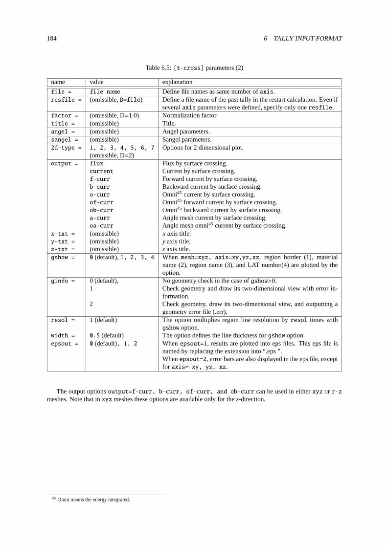
184 6 TALLY INPUT FORMAT
Table 6.5:[t-cross] parameters (2)
name value explanation
file = file name Define file names as same number ofaxis.resfile = (omissible,D=file) Define a file name of the past tally in the restart calculation. Even if
severalaxis parameters were defined, specify only oneresfile.factor = (omissible, D=1.0) Normalization factor.title = (omissible) Title.angel = (omissible) Angel parameters.sangel = (omissible) Sangel parameters.2d-type = 1, 2, 3, 4, 5, 6, 7 Options for 2 dimensional plot.
(omissible, D=2)output = flux Flux by surface crossing.
current Current by surface crossing.f-curr Forward current by surface crossing.b-curr Backward current by surface crossing.o-curr Omni45 current by surface crossing.of-curr Omni45 forward current by surface crossing.ob-curr Omni45 backward current by surface crossing.a-curr Angle mesh current by surface crossing.oa-curr Angle mesh omni45 current by surface crossing.
x-txt = (omissible) x axis title.y-txt = (omissible) y axis title.z-txt = (omissible) z axis title.gshow = 0 (default),1, 2, 3, 4 When mesh=xyz, axis=xy,yz,xz, region border (1), material
name (2), region name (3), and LAT number(4) are plotted by theoption.
ginfo = 0 (default), No geometry check in the case ofgshow>0.1 Check geometry and draw its two-dimensional view with error in-
formation.2 Check geometry, draw its two-dimensional view, and outputting a
geometry error file (.err).resol = 1 (default) The option multiplies region line resolution byresol times with
gshow option.width = 0.5 (default) The option defines the line thickness forgshow option.epsout = 0 (default), 1, 2 Whenepsout=1, results are plotted into eps files. This eps file is
named by replacing the extension into “.eps ”.Whenepsout=2, error bars are also displayed in the eps file, exceptfor axis= xy, yz, xz.
The output optionsoutput=f-curr, b-curr, of-curr, and ob-curr can be used in eitherxyz or r-zmeshes. Note that inxyz meshes these options are available only for thez-direction.
45 Omni means the energy integrated.

6.2 [ T-Cross ] section 185
Table 6.6:[t-cross] parameters (3)
name value explanation
ctmin(i) = (omissible, D=-9999) Minimum value fori-th counter.ctmax(i) = (omissible, D= 9999) Maximum value fori-th counter.trcl = (omissible) Coordinate transformation number or definition forr-z or xyz
mesh.dump = Number of data For mesh=reg, the information is dumped on the file. Ifdump is
negative, data are written by ascii, if positive, by binary.(next line) Data sequence Define the data sequence. The history information (nocas and
nobch) is necessary to useidmpmode=1.gslat = 1(default), 0 1: show lattice boundary in gshow, 0: no.stdcut = (omissible,D=-1) Threshold value of STD cut off.multiplier = Number of material Multiplier for each material.
(omissible) Multiplier subsection is required below this parameter.
In the [t-cross] tally, the dump option can only be used with reg meshes and only onaxis=reg. If thedump option is set, thee-type, a-type andt-type meshes take on only the maximum and minimum values.The output option can be set ascurrent, a-curr, or oa-curr. In using this dump parameter,axis andfileare restricted to one axis and one file apiece and unit is always 1. The dumped data are written onto a file named“*** dmp”, where “***” indicates the file name specified byfile=***. The normal output of the tally is writtenon “***”. From this file, information on the total normalization factor can be obtained; doing so requires settingone mesh each fore-type, a-type andt-type (in the versions of PHITS before 2.66, the normal output waswritten on a configuration file (.cfg) and the dumped data were written on “***”). The history information (nocas
andnobch) is necessary to useidmpmode=1 for continuous calculation using the dump file; in addition, both thedump file with “ dmp” and the normal output file specified byfile= are required to useidmpmode=1. The optiondumpall is not compatible with this dump tally option when shared memory parallelization is active.
By specifyingstdcut, you can automatically stop a PHITS calculation depending on values of STD (standarddeviation). This function is available whenstdcut is positive anditall=0,1 is set in[parameters] section.When all relative values of STD of the tally result are smaller thanstdcut at the last of one batch, PHITS finishesits calculation. If you setstdcut in two (or more) tally sections, all the results of the tally sections have to satisfythe conditions in order to work the function.
From ver. 2.86,multiplier option can be used in[t-cross] tally.Usingmultiplier option in this tally, you can multiply results of the tally by factors depending on energies
of particles. If you define a data set in[multiplier] section, any factors can be used. The basic format is givenas (C k), whereC is a normalization factor andk is the ID number of the set. It is noted thatk should be negative.Format of themultiplier subsection is given as follows.
multiplier = number of materialpart = neutron
emax = 1000
mat mset1 mset2
1 ( 1 -201 ) ( 2 -202 )
2 ( 1.2 -201 ) ( 3 -202 )
.... .... .... ....
.... .... .... ....
The line ofmultiplier = specifies the number of material where the multiplication is considered. You can useall instead of the number. For this case, one should also useall for mat column below. The second line ofpart= defines the particles considered. The maximum number of the particle is 6 andall can be also used, which isdefault. The multiplication affects only these considered particles. The third line ofemax = defines the maximumenergy of the multiplication. Ifemax is omitted, it is automatically defined as the maximum energy given in the

186 6 TALLY INPUT FORMAT
[multiplier] section, ordmax(i), i = 1, 2, or 14 when you use nuclear data library. The number ofmatcolumn is the material number which is considered to be multiplied. The columns ofmset1, mset2 define themultiplier set. The maximum 6 multiplier can be set. For each set, the result is printed out. You can define severalmultiplier subsections in one[t-cross] section, but you should set the number of the multiplier sets to beequal in each subsection.
Some parameter sets built-in PHITS can be used. If you setk = −1, a value of 1/weight is used as themultiplication factor. Fork = −2, a value of 1/velocity is used. Fork = −120, material density is used. Therefore,you can obtain mass in the region settingicntl=5. With k = −101,−102,−112, or−114, the conversion factor ofproton, neutron, electron, or photon, respectively, is used. These conversion factors were estimated with a conditionof Antero-Posterior geometry (AP) irradiation.?) The unit of the dose conversion factors is (µSv/h)/(n/sec/cm2). Itshould be noted that the interpolation method of conversion factor has been changed in PHITS ver. 2.00 fromlinear-linear to log-log.
You can also use the following format.
multiplier = number of materialpart = proton
emax = 150
mat mset1 mset2
1 ( 0.1236 1 1 -4 ) ( 0.0 )
2 ( 0.0060 2 1 -4 ) ( 0.0 )
3 ( 0.0032 3 1 -4 ) ( 0.0 )
.... .... .... ....
.... .... .... ....
multiplier = number of materialpart = neutron
emax = 150
mat mset1 mset2
1 ( 0.1236 1 1 -4 : -6 -8 ) ( 1.0 -1 33 0.543 )
2 ( 0.0060 2 1 -4 : -6 -8 ) ( 1.0 -1 34 0.321 )
3 ( 0.0032 3 1 -4 : -6 -8 ) ( 1.0 -1 35 0.678 )
.... .... .... ....
.... .... .... ....
In above example, themset1 is for heat and themset2 is zero for proton, attenuator set for neutron.

6.2 [ T-Cross ] section 187
Settingmesh=reg for the geometry mesh in this section requires defining the crossing surface by outgoing(r-from) and incoming (r-to) region number, and the area of the surface (area in units of cm2), as shown in theexample below46.
mesh = reg
reg = number of crossing surfacesr-from r-to area
2 8 10.0
3 8 5.0
( 4 5 ) ( 4 5 ) 2.0
(13<5) (14<5) 7.0
(13<6) (14<6) 7.0
(13<7) (14<7) 7.0
... ... ....
... ... ....
In the next line ofmesh=reg, give the number of crossing surfaces to tally byreg=. Furthermore, from the nextline, the values ofr-in r-out, andarea should be written as a matrix format. The default order for this definitionis r-in r-out area. The line of these column headers can be omitted. However, to change the order, rearrangeand explicitly write the column headers asr-in r-out area. The skip operatornon can be also used. Whenspecifying the region number, the format( 2 -5 8 9 ) can be used, as can the lattice and universe style( 6 <
10[1 0 0] < u=3 ). However, any value that is not single numeric must be enclosed by( ) .If mesh=reg is set, the obtained current or flux is unidirectional fromr-from to r-to; a bidirectional flux can
be set in the third line of the above definition.Setting themesh=r-z defines the numbers of two crossing surface types: the number of “nz+1” crossing
surfaces forz defined byr i − r i+1 and the number of “nr+1” crossing surfaces forr defined byzi − zi+1. If anr-surface coincides with the surface of the outer void, the flux on this surface is not tallied.
If mesh=xyz is set, the number of “nz+1” crossing surfaces onzare defined byxi − xi+1, andy j − y j+1. In thiscase,x andy crossing surfaces are not defined. Settingmesh=r-z or xyz causes crossing particles to be detectedin both directions on the defined surface. The forward direction is defined as the positive direction on az surfaceand from the center to the exterior on anr surface.
46 Before ver. 2.96,r-in andr-out were used instead ofr-from andr-to, respectively. These old parameters can be used after ver. 2.97.Note that “in” and “out” are reversed in this definition.

188 6 TALLY INPUT FORMAT
6.3 [ T-Point ] section
It is impractical to calculate particle fluence at a certain point or line, using[t-track] tally. Hence, the pointestimator tally[t-point] was introduced to estimate such quantities in a short computational time. However, thefollowing conditions must be satisfied in the PHITS simulation using[t-point]:
(1) Particle energy should not exceed the maximum energy of the data library used, i.e.dmax.
(2) Only fluence of neutron and photon can be calculated by[t-point].
(3) Neither event generator mode nor EGS5 should not be used (e-mode=0, negs=0).
(4) Material should be uniform within a certain distance around the point detector due to singularity.
(5) Reflection or white boundary surface should not be used.
Please see read-me file or sample input file in\phits\utility\tpoint in more detail.
Table 6.7:[t-point] parameters(1)
name value explanation
point = number of data Option for point detectors.
You need subsection below this parameter.
ring = number of data Option for ring detectors.
You need subsection below this parameter.
part = all (default), maximum 6 particles in a [t-point]
particle name
e-type = 1, 2, 3, 4, 5 energy mesh
You need energy mesh subsection below this option
t-type = 1, 2, 3, 4, 5 time mesh
(omissible) You need time mesh subsection below this option
unit = 1, 2, 3 1: [1/cm2/source]
2: [1/cm2/MeV/source]
3: [1/cm2/Lethargy/source]
11, 12, 13 11:[1/cm2/nsec/source]
12:[1/cm2/nsec/MeV/source]
13:[1/cm2/Lethargy/nsec/source]
axis = eng, t x axis of output data
file = file name Define file names as same number of axis
resfile = (omissible, D=file) Define a file name of the past tally in the
restart calculation. Even if several axis
parameters were defined, you should specify only
one resfile.
factor = (omissible, D=1.0) normalization factor
title = (omissible) title
angel = (omissible) angel parameters
sangel = (omissible) sangel parameters
epsout = 0 (default), 1, 2 When epsout=1, results are plotted into eps files.
This eps file is named by replacing the extension
into ‘‘.eps ’’.
When epsout=2, error bars are also displayed in
the eps file.
ctmin(i) = (omissible, D=-9999) minimum value for i-th counter
ctmax(i) = (omissible, D= 9999) maximum value for i-th counter
“Lethargy ” in unit = 3 or 13 is a natural logarithmic unit of energy, and defined by ln(Eref/E) using areference energyEref and a particle’s energyE. If you set these units, you can obtain results per Lethargy, which
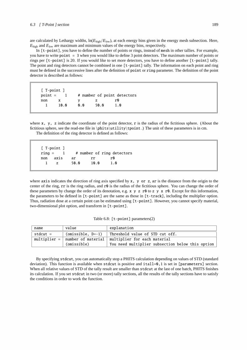
6.3 [ T-Point ] section 189
are calculated by Lethargy widths, ln(Ehigh/Elow), at each energy bins given in the energy mesh subsection. Here,Ehigh andElow are maximum and minimum values of the energy bins, respectively.
In [t-point], you have to define the number of points or rings, instead ofmesh in other tallies. For example,you have to writepoint = 3 when you would like to define 3 point detectors. The maximum number of points orrings per[t-point] is 20. If you would like to set more detectors, you have to define another[t-point] tally.The point and ring detectors cannot be combined in one[t-point] tally. The information on each point and ringmust be defined in the successive lines after the definition ofpoint or ring parameter. The definition of the pointdetector is described as follows:
[ T-point ]
point = 1 # number of point detectors
non x y z r0
1 10.0 0.0 50.0 1.0
wherex, y, z indicate the coordinate of the point detector,r is the radius of the fictitious sphere. (About thefictitious sphere, see the read-me file in\phits\utility\tpoint .) The unit of these parameters is in cm.
The definition of the ring detector is defined as follows:
[ T-point ]
ring = 1 # number of ring detectors
non axis ar rr r0
1 z 50.0 10.0 1.0
whereaxis indicates the direction of ring axis specified byx, y or z, ar is the distance from the origin to thecenter of the ring,rr is the ring radius, andr0 is the radius of the fictitious sphere. You can change the order ofthese parameters by change the order of its denotation, e.g.x y z r0 to z y x r0. Except for this information,the parameters to be defined in[t-point] are the same as those in[t-track], including the multiplier option.Thus, radiation dose at a certain point can be estimated using[t-point]. However, you cannot specify material,two-dimensional plot option, and transform in[t-point].
Table 6.8:[t-point] parameters(2)
name value explanation
stdcut = (omissible, D=-1) Threshold value of STD cut off.
multiplier = number of material multiplier for each material
(omissible) You need multiplier subsection below this option
By specifyingstdcut, you can automatically stop a PHITS calculation depending on values of STD (standarddeviation). This function is available whenstdcut is positive anditall=0,1 is set in[parameters] section.When all relative values of STD of the tally result are smaller thanstdcut at the last of one batch, PHITS finishesits calculation. If you setstdcut in two (or more) tally sections, all the results of the tally sections have to satisfythe conditions in order to work the function.

190 6 TALLY INPUT FORMAT
Usingmultiplier option in this tally, you can multiply results of the[t-point] tally by factors dependingon energies of particles. If you define a data set in[multiplier] section, any factors can be used. The basicformat is given as (C k), whereC is a normalization factor andk is the ID number of the set. It is noted thatkshould be negative. Format of themultiplier subsection is given as follows.
multiplier = number of materialpart = neutron
emax = 1000
mat mset1 mset2
1 ( 1 -201 ) ( 2 -202 )
2 ( 1.2 -201 ) ( 3 -202 )
.... .... .... ....
.... .... .... ....
The line ofmultiplier = specifies the number of material where the multiplication is considered. You can useall instead of the number. For this case, one should also useall for mat column below. The second line ofpart= defines the particles considered. The maximum number of the particle is 6 andall can be also used, which isdefault. The multiplication affects only these considered particles. The third line ofemax = defines the maximumenergy of the multiplication. Ifemax is omitted, it is automatically defined as the maximum energy given in the[multiplier] section, ordmax(i), i = 1, 2, or 14 when you use nuclear data library. The number ofmatcolumn is the material number which is considered to be multiplied. The columns ofmset1, mset2 define themultiplier set. The maximum 6 multiplier can be set. For each set, the result is printed out. You can define severalmultiplier subsections in one[t-point] section, but you should set the number of the multiplier sets to beequal in each subsection.
Some parameter sets built-in PHITS can be used. If you setk = −1, a value of 1/weight is used as themultiplication factor. Fork = −2, a value of 1/velocity is used. Fork = −120, material density is used. Therefore,you can obtain mass in the region settingicntl=5. With k = −101,−102,−112, or−114, the conversion factor ofproton, neutron, electron, or photon, respectively, is used. These conversion factors were estimated with a conditionof Antero-Posterior geometry (AP) irradiation.?) The unit of the dose conversion factors is (µSv/h)/(n/sec/cm2). Itshould be noted that the interpolation method of conversion factor has been changed in PHITS ver. 2.00 fromlinear-linear to log-log.
You can also use the following format.
multiplier = number of materialpart = proton
emax = 150
mat mset1 mset2
1 ( 0.1236 1 1 -4 ) ( 0.0 )
2 ( 0.0060 2 1 -4 ) ( 0.0 )
3 ( 0.0032 3 1 -4 ) ( 0.0 )
.... .... .... ....
.... .... .... ....
multiplier = number of materialpart = neutron
emax = 150
mat mset1 mset2
1 ( 0.1236 1 1 -4 : -6 -8 ) ( 1.0 -1 33 0.543 )
2 ( 0.0060 2 1 -4 : -6 -8 ) ( 1.0 -1 34 0.321 )
3 ( 0.0032 3 1 -4 : -6 -8 ) ( 1.0 -1 35 0.678 )
.... .... .... ....
.... .... .... ....
In above example, themset1 is for heat and themset2 is zero for proton, attenuator set for neutron.
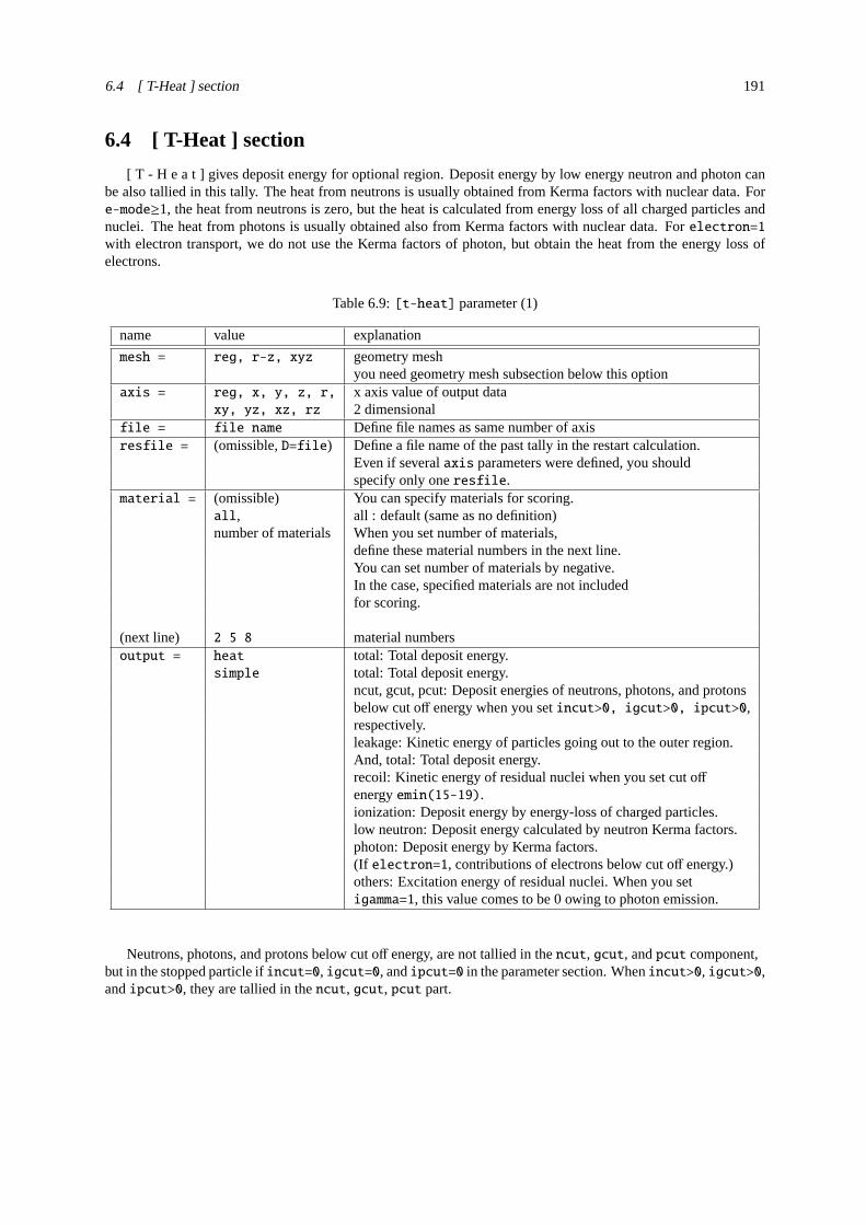
6.4 [ T-Heat ] section 191
6.4 [ T-Heat ] section
[ T - H e a t ] gives deposit energy for optional region. Deposit energy by low energy neutron and photon canbe also tallied in this tally. The heat from neutrons is usually obtained from Kerma factors with nuclear data. Fore-mode≥1, the heat from neutrons is zero, but the heat is calculated from energy loss of all charged particles andnuclei. The heat from photons is usually obtained also from Kerma factors with nuclear data. Forelectron=1
with electron transport, we do not use the Kerma factors of photon, but obtain the heat from the energy loss ofelectrons.
Table 6.9:[t-heat] parameter (1)
name value explanation
mesh = reg, r-z, xyz geometry meshyou need geometry mesh subsection below this option
axis = reg, x, y, z, r, x axis value of output dataxy, yz, xz, rz 2 dimensional
file = file name Define file names as same number of axisresfile = (omissible,D=file) Define a file name of the past tally in the restart calculation.
Even if severalaxis parameters were defined, you shouldspecify only oneresfile.
material = (omissible) You can specify materials for scoring.all, all : default (same as no definition)number of materials When you set number of materials,
define these material numbers in the next line.You can set number of materials by negative.In the case, specified materials are not includedfor scoring.
(next line) 2 5 8 material numbersoutput = heat total: Total deposit energy.
simple total: Total deposit energy.ncut, gcut, pcut: Deposit energies of neutrons, photons, and protonsbelow cut off energy when you setincut>0, igcut>0, ipcut>0,respectively.leakage: Kinetic energy of particles going out to the outer region.And, total: Total deposit energy.recoil: Kinetic energy of residual nuclei when you set cut offenergyemin(15-19).ionization: Deposit energy by energy-loss of charged particles.low neutron: Deposit energy calculated by neutron Kerma factors.photon: Deposit energy by Kerma factors.(If electron=1, contributions of electrons below cut off energy.)others: Excitation energy of residual nuclei. When you setigamma=1, this value comes to be 0 owing to photon emission.
Neutrons, photons, and protons below cut off energy, are not tallied in thencut, gcut, andpcut component,but in the stopped particle ifincut=0, igcut=0, andipcut=0 in the parameter section. Whenincut>0, igcut>0,andipcut>0, they are tallied in thencut, gcut, pcut part.
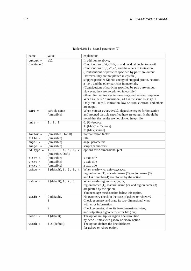
192 6 TALLY INPUT FORMAT
Table 6.10:[t-heat] parameter (2)
name value explanation
output = all In addition to above,(continued) Contributions ofd, t,3He,α, and residual nuclei to recoil.
Contributions ofp, π+, π−, and the others to ionization.(Contributions of particles specified bypart are output.However, they are not plotted in eps file.)stopped particle: Kinetic energy of stopped proton, neutron,π+, π−, and the other particles in materials.(Contributions of particles specified bypart are output.However, they are not plotted in eps file.)others: Remaining excitation energy and fission component.Whenaxis is 2 dimensional,all is the same assimple.Only total, recoil, ionization, low neutron, electron, and othersare output.
part = particle name When you setoutput=all, deposit energies for ionization(omissible) and stopped particle specified here are output. It should be
noted that the results are not plotted in eps file.unit = 0, 1, 2 0: [Gy/source]
1: [MeV/cm3/source]2: [MeV/source]
factor = (omissible, D=1.0) normalization factortitle = (omissible) titleangel = (omissible) angel parameterssangel = (omissible) sangel parameters2d-type = 1, 2, 3, 4, 5, 6, 7 options for 2 dimensional plot
(omissible, D=3)x-txt = (omissible) x axis titley-txt = (omissible) y axis titlez-txt = (omissible) z axis titlegshow = 0 (default),1, 2, 3, 4 When mesh=xyz, axis=xy,yz,xz,
region border (1), material name (2), region name (3),and LAT number(4) are plotted by the option.
rshow = 0 (default),1, 2, 3 When mesh=reg, axis=xy,yz,xz,region border (1), material name (2), and region name (3)are plotted by the option.You need xyz mesh section below this option.
ginfo = 0 (default), No geometry check in the case of gshow or rshow>01 Check geometry and draw its two-dimensional view
with error information2 Check geometry, draw its two-dimensional view,
and outputting a geometry error file (.err)resol = 1 (default) The option multiplies region line resolution
by resol times with gshow or rshow option.width = 0.5 (default) The option defines the line thickness
for gshow or rshow option.

6.4 [ T-Heat ] section 193
Generally speaking, heat is an energy of ionization of charged particles. However, in the transport simulation,cutoff energy of the particle is set and the transport is stopped below the energy. Then there exist some componentsof heat, i.e. recoil, stopped particle, and others, in the output of the heat tally. These components may change asthe parameters of the transport are changed.
Table 6.11:[t-heat] parameter (3)
name value explanation
volume (omissible) The option defines volume for each regionfor reg mesh. You need volume definitionsbelow this option.Default values are given in inputecho in the case of no definition.
reg vol volume definition. See5.1.2iechrl = 72 (default) Number of maximum column for volume input echovolmat = (omissible, D=9) The option corrects a volume value for each mesh
when material is defined by xyz mesh.(0 means no correction)Value of volmat means the number of scansfor one side of xyz mesh
epsout = 0 (default), 1, 2 Whenepsout=1, results are plotted into eps files.This eps file is named by replacing the extension into “.eps ”.Whenepsout=2, error bars are also displayed in the eps file,except foraxis= xy, yz, xz, rz.
bmpout = 0(default), 1 Generate Bitmap figure of 2-dimensional tally output.This file is named by replacing the extension into “.bmp ”.Whenmesh=xyz, axis=(xy, yz, or xz), this is available.
vtkout = 0(default), 1 Output the tally results in xyz-mesh in the input format of ParaView.This file is named by replacing the extension into “.vtk ”.Whenmesh=xyz, axis=(xy, yz, or xz), this is available.
vtkfmt = 0(default), 1 Format of output file for ParaView.0: ascii, 1: binary.
electron = 0 (default),1 electron contribution options0: using photon KERMA factors(electron and positron should NOT be transported,otherwise their deposition energies are double counted)1: calculating by ionization loss(electron and positron transports are required)
ctmin(i) = (omissible, D=-9999) minimum value for i-th counterctmax(i) = (omissible, D= 9999) maximum value for i-th countertrcl = (omissible) coordinate transformation number or definition
for r-z or xyz meshgslat = 1(default), 0 1: show lattice boundary in gshow, 0: nostdcut = (omissible,D=-1) Threshold value of STD cut off.
When you setunit = 0, you can obtain results in the unit of [Gy/source]. When you setmesh = reg, youshould define volumes of each cells in [volume] section or by settingvolume parameter of the [t-heat] section.Because absorbed dose is intensive variable, PHITS does not output “sum over”in output files forunit = 0. Itshould be noted that when a region includes more than two materials, dose in the region does not equal to averagevalue of the region. For example, when two material with massesM1 & M2, and absorb energiesE1 & E2,respectively, PHITS givesE1
M1+ E2
M2in this tally, though its average dose isE1+E2
M1+M2.
By specifyingstdcut, you can automatically stop a PHITS calculation depending on values of STD (standarddeviation). This function is available whenstdcut is positive anditall=0,1 is set in[parameters] section.When all relative values of STD of the tally result are smaller thanstdcut at the last of one batch, PHITS finishesits calculation. If you setstdcut in two (or more) tally sections, all the results of the tally sections have to satisfythe conditions in order to work the function.

194 6 TALLY INPUT FORMAT
6.5 [ T-Deposit ] section
This tally is very similar to[t-heat] and scores dose and deposit energy distributions. The difference from[t-heat] is that this tally only counts an energy loss of charged particles and nuclei. Thus, you must use the eventgenerator mode (e-mode≥1) if you would like to transport low-energy neutrons. In this tally, you can multiply anyfactor as a function of LET(dE/dx) in a certain material to the dose or deposit energy. This function is realizedby user defined subroutine usrdfn1.f and usrdn2.f. As examples, the default program of usrdfn1.f returns the doseequivalent calculated from deposit energy multiplied with theQ(L) relationship defined in the ICRP60, while thatof usrdfn2.f estimates biological dose on the basis of Microdosimetric Kinetic Model47. You can change and addany factor in this routine. Note thatletmat should be set to water when these default programs are used (see“particle therapy” in the recommendation setting in more detail). In addition, using the time mesh with[timer]
section, you can simulate a TOF (time of flight) detector and plot 2-dimensional graph of the correlation betweenthe deposit energy and the TOF. Whenoutput = deposit is set, you can simulate the detector response. Notethat you cannot use this tally when a particle weight changes in the calculation by using[weight window] etc.After version 2.70, the detector resolution can be considered in the calculation of event-by-event deposition-energydistributions usingoutput = deposit.
Table 6.12:[t-deposit] parameters (1)
name value explanation
mesh = reg, r-z, xyz Geometry mesh.A geometry mesh subsection is required below this option.
part = all (default), Maximum 6 particles in a[t-deposit].particle name Whenoutput=deposit anddeposit=0, all is necessary and only
maximum 5 particles can be set.material = (omissible) Materials to score can be specified.
all, all : default (same as no definition)number of materials When you set number of materials, define these material numbers in the
next line. You can set number of materials by negative. In the case,specified materials are not included for scoring.
(next line) 2 5 8 Material numbers.letmat = (omissible) Material id for LET(dE/dx).
If omitted, a real material is assumed.If a material not used in the geometry is selected, its material densitymust be defined in[material]. To calculate LET in water, definewater with 1 g/cm3 in [material].Whenletmat<0 is set, PHITS automatically calculatesdE/dx for wa-ter with 1 g/cm3 for electrons and positrons: please see “particle ther-apy” in the recommendation setting for more details.
dedxfnc = (omissible, D=0) 0: without, 1: use usrdfn1.f, 2: use usrdfn2.f.As examples, the default program of usrdfn1.f returns the dose equiva-lent calculated from deposit energy multiplied by theQ(L) relationshipdefined in the ICRP60, while that of usrdfn2.f estimates biological doseon the basis of Microdosimetric Kinetic Model.
e-type = 1, 2, 3, 4, 5 Energy mesh.An energy mesh subsection is required below this option.
t-type = 1, 2, 3, 4, 5 Time mesh.(omissible) A time mesh subsection is required below this option.
47 T.Sato et al. Biological dose estimation for charged-particle therapy using an improved PHITS code coupled with a microdosimetrickinetic model, Radiat. Res. 171, 107-117 (2009).
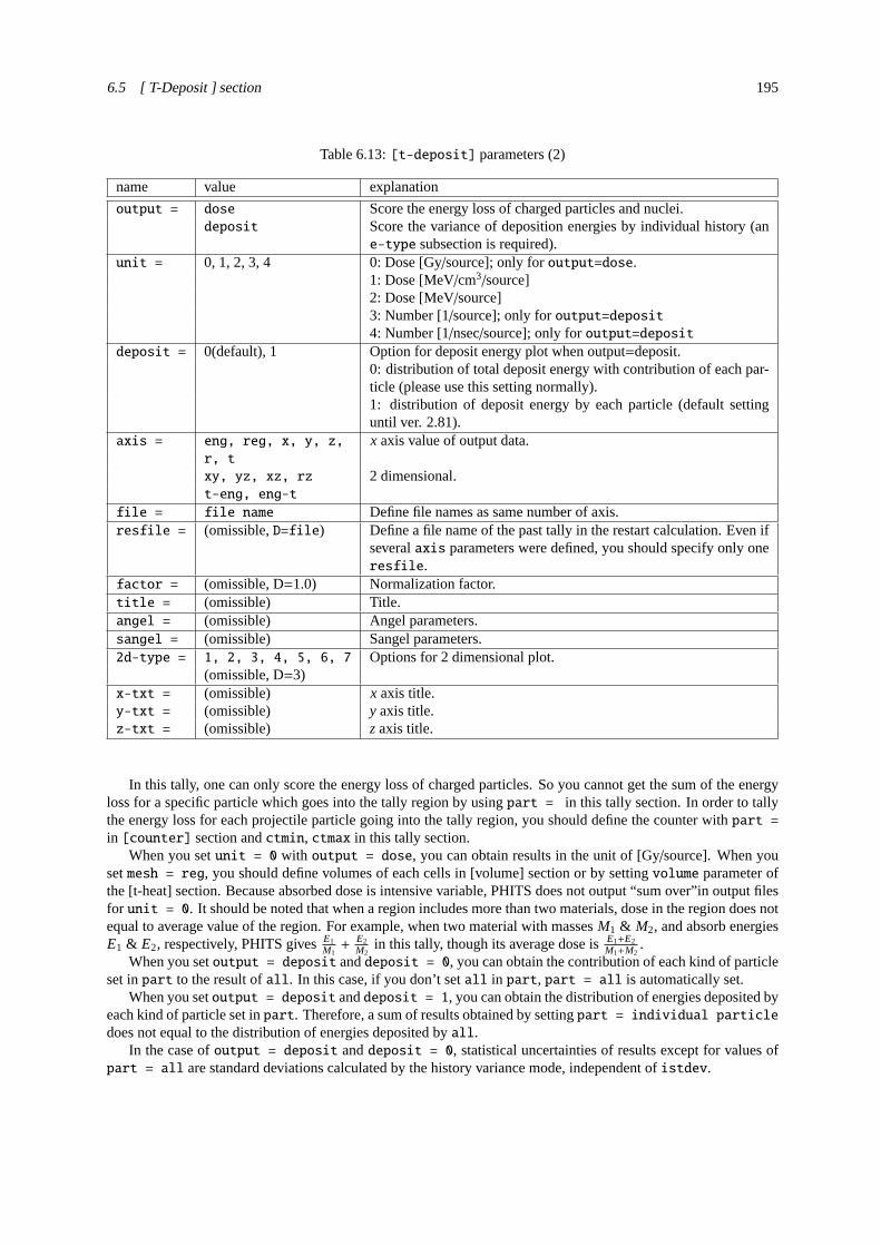
6.5 [ T-Deposit ] section 195
Table 6.13:[t-deposit] parameters (2)
name value explanation
output = dose Score the energy loss of charged particles and nuclei.deposit Score the variance of deposition energies by individual history (an
e-type subsection is required).unit = 0, 1, 2, 3, 4 0: Dose [Gy/source]; only foroutput=dose.
1: Dose [MeV/cm3/source]2: Dose [MeV/source]3: Number [1/source]; only foroutput=deposit4: Number [1/nsec/source]; only foroutput=deposit
deposit = 0(default), 1 Option for deposit energy plot when output=deposit.0: distribution of total deposit energy with contribution of each par-ticle (please use this setting normally).1: distribution of deposit energy by each particle (default settinguntil ver. 2.81).
axis = eng, reg, x, y, z, x axis value of output data.r, t
xy, yz, xz, rz 2 dimensional.t-eng, eng-t
file = file name Define file names as same number of axis.resfile = (omissible,D=file) Define a file name of the past tally in the restart calculation. Even if
severalaxis parameters were defined, you should specify only oneresfile.
factor = (omissible, D=1.0) Normalization factor.title = (omissible) Title.angel = (omissible) Angel parameters.sangel = (omissible) Sangel parameters.2d-type = 1, 2, 3, 4, 5, 6, 7 Options for 2 dimensional plot.
(omissible, D=3)x-txt = (omissible) x axis title.y-txt = (omissible) y axis title.z-txt = (omissible) z axis title.
In this tally, one can only score the energy loss of charged particles. So you cannot get the sum of the energyloss for a specific particle which goes into the tally region by usingpart = in this tally section. In order to tallythe energy loss for each projectile particle going into the tally region, you should define the counter withpart =
in [counter] section andctmin, ctmax in this tally section.When you setunit = 0 with output = dose, you can obtain results in the unit of [Gy/source]. When you
setmesh = reg, you should define volumes of each cells in [volume] section or by settingvolume parameter ofthe [t-heat] section. Because absorbed dose is intensive variable, PHITS does not output “sum over”in output filesfor unit = 0. It should be noted that when a region includes more than two materials, dose in the region does notequal to average value of the region. For example, when two material with massesM1 & M2, and absorb energiesE1 & E2, respectively, PHITS givesE1
M1+ E2
M2in this tally, though its average dose isE1+E2
M1+M2.
When you setoutput = deposit anddeposit = 0, you can obtain the contribution of each kind of particleset inpart to the result ofall. In this case, if you don’t setall in part, part = all is automatically set.
When you setoutput = deposit anddeposit = 1, you can obtain the distribution of energies deposited byeach kind of particle set inpart. Therefore, a sum of results obtained by settingpart = individual particledoes not equal to the distribution of energies deposited byall.
In the case ofoutput = deposit anddeposit = 0, statistical uncertainties of results except for values ofpart = all are standard deviations calculated by the history variance mode, independent ofistdev.

196 6 TALLY INPUT FORMAT
Table 6.14:[t-deposit] parameters (3)
name value explanation
gshow = 0 (default),1, 2, 3, 4 When mesh=xyz, axis=xy,yz,xz,region border (1), material name (2), region name (3),and LAT number(4) are plotted by the option.
rshow = 0 (default),1, 2, 3 When mesh=reg, axis=xy,yz,xz,region border (1), material name (2), and region name (3)and LAT number(4) are plotted by the option.You need xyz mesh section below this option.
ginfo = 0 (default), No geometry check in the case of gshow or rshow>01 Check geometry and draw its two-dimensional view
with error information2 Check geometry, draw its two-dimensional view,
and outputting a geometry error file (.err)resol = 1 (default) The option multiplies region line resolution
by resol times with gshow or rshow option.width = 0.5 (default) The option defines the line thickness
for gshow or rshow option.volume (omissible) The option defines volume for each region for reg mesh.
You need volume definitions below this option. Defaultvalues are given in input echo in the case of no definition.
reg vol volume definition. See5.1.2iechrl = 72 (default) Number of maximum column for volume input echovolmat = (omissible, D=9) The option corrects a volume value for each mesh
when material is defined by xyz mesh.(0 means no correction)Value of volmat means the number of scansfor one side of xyz mesh
epsout = 0 (default), 1, 2 Whenepsout=1, results are plotted into eps files.This eps file is named by replacing the extension into “.eps ”.Whenepsout=2, error bars are also displayed in the eps file,except foraxis= xy, yz, xz, rz, t-eng, eng-t.
bmpout = 0(default), 1 Generate Bitmap figure of 2-dimensional tally output.This file is named by replacing the extension into “.bmp ”.Whenmesh=xyz, axis=(xy, yz, or xz), this is available.
vtkout = 0(default), 1 Output the tally results in xyz-mesh in the input format of ParaView.This file is named by replacing the extension into “.vtk ”.Whenmesh=xyz, axis=(xy, yz, or xz), this is available.
vtkfmt = 0(default), 1 Format of output file for ParaView.0: ascii, 1: binary.
ctmin(i) = (omissible, D=-9999) minimum value for i-th counterctmax(i) = (omissible, D= 9999) maximum value for i-th countertrcl = (omissible) coordinate transformation number or definition
for r-z or xyz meshgslat = 1(default), 0 1: show lattice boundary in gshow, 0: no
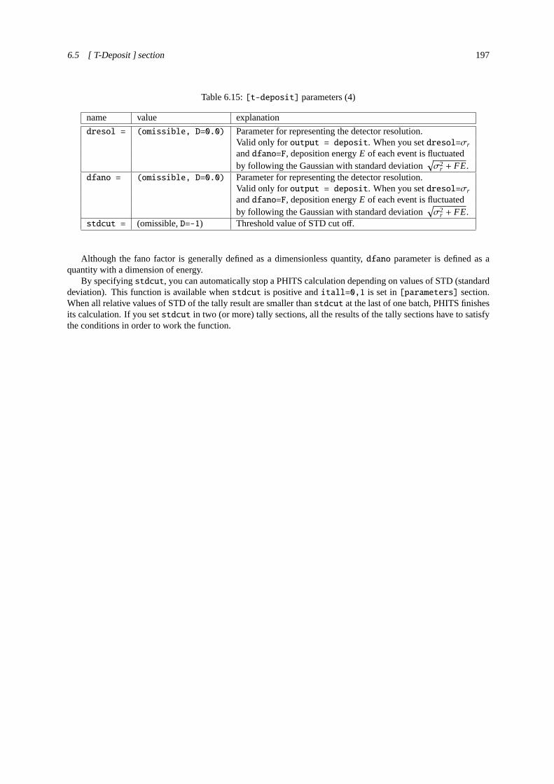
6.5 [ T-Deposit ] section 197
Table 6.15:[t-deposit] parameters (4)
name value explanation
dresol = (omissible, D=0.0) Parameter for representing the detector resolution.Valid only for output = deposit. When you setdresol=σr
anddfano=F, deposition energyE of each event is fluctuatedby following the Gaussian with standard deviation
√σ2
r + FE.dfano = (omissible, D=0.0) Parameter for representing the detector resolution.
Valid only for output = deposit. When you setdresol=σr
anddfano=F, deposition energyE of each event is fluctuatedby following the Gaussian with standard deviation
√σ2
r + FE.stdcut = (omissible,D=-1) Threshold value of STD cut off.
Although the fano factor is generally defined as a dimensionless quantity,dfano parameter is defined as aquantity with a dimension of energy.
By specifyingstdcut, you can automatically stop a PHITS calculation depending on values of STD (standarddeviation). This function is available whenstdcut is positive anditall=0,1 is set in[parameters] section.When all relative values of STD of the tally result are smaller thanstdcut at the last of one batch, PHITS finishesits calculation. If you setstdcut in two (or more) tally sections, all the results of the tally sections have to satisfythe conditions in order to work the function.
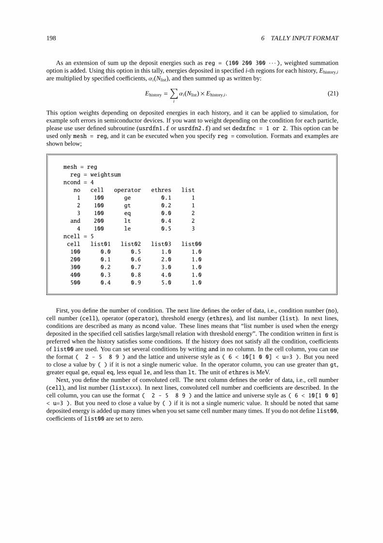
198 6 TALLY INPUT FORMAT
As an extension of sum up the deposit energies such asreg = (100 200 300 · · · ), weighted summationoption is added. Using this option in this tally, energies deposited in specifiedi-th regions for each history,Ehistory,i
are multiplied by specified coefficients,αi(Nlist), and then summed up as written by:
Ehistory =∑
i
αi(Nlist) × Ehistory,i . (21)
This option weights depending on deposited energies in each history, and it can be applied to simulation, forexample soft errors in semiconductor devices. If you want to weight depending on the condition for each particle,please use user defined subroutine (usrdfn1.f or usrdfn2.f) and setdedxfnc = 1 or 2. This option can beused onlymesh = reg, and it can be executed when you specifyreg = convolution. Formats and examples areshown below;
mesh = reg
reg = weightsum
ncond = 4
no cell operator ethres list
1 100 ge 0.1 1
2 100 gt 0.2 1
3 100 eq 0.0 2
and 200 lt 0.4 2
4 100 le 0.5 3
ncell = 5
cell list01 list02 list03 list00
100 0.0 0.5 1.0 1.0
200 0.1 0.6 2.0 1.0
300 0.2 0.7 3.0 1.0
400 0.3 0.8 4.0 1.0
500 0.4 0.9 5.0 1.0
First, you define the number of condition. The next line defines the order of data, i.e., condition number (no),cell number (cell), operator (operator), threshold energy (ethres), and list number (list). In next lines,conditions are described as many asncond value. These lines means that “list number is used when the energydeposited in the specified cell satisfies large/small relation with threshold energy”. The condition written in first ispreferred when the history satisfies some conditions. If the history does not satisfy all the condition, coefficientsof list00 are used. You can set several conditions by writingand in no column. In the cell column, you can usethe format( 2 - 5 8 9 ) and the lattice and universe style as( 6 < 10[1 0 0] < u=3 ). But you needto close a value by( ) if it is not a single numeric value. In the operator column, you can use greater thangt,greater equalge, equaleq, less equalle, and less thanlt. The unit ofethres is MeV.
Next, you define the number of convoluted cell. The next column defines the order of data, i.e., cell number(cell), and list number (listxxxx). In next lines, convoluted cell number and coefficients are described. In thecell column, you can use the format( 2 - 5 8 9 ) and the lattice and universe style as( 6 < 10[1 0 0]< u=3 ). But you need to close a value by( ) if it is not a single numeric value. It should be noted that samedeposited energy is added up many times when you set same cell number many times. If you do not definelist00,coefficients oflist00 are set to zero.

6.6 [ T-Deposit2 ] section 199
6.6 [ T-Deposit2 ] section
This tally scores deposit energy distribution in two regions and plot the correlation between two deposit ener-gies. By this, one can simulate, for an example, dE, E counters and plot the correlations in 2-dimensional graph.Using this tally, you can simulate the detector response. Note that you cannot use this tally when a particle weightchanges in the calculation by using[weight window] etc. In this tally, as in the [t-deposit] tally, you can multiplyany factor as a function of LET(dE/dx) in a certain material to the dose or deposit energy. This function is realizedby user defined subroutine usrdfn1.f and usrdn2.f. As examples, the default program of usrdfn1.f returns the doseequivalent calculated from deposit energy multiplied with theQ(L) relationship defined in the ICRP60, while thatof usrdfn2.f estimates biological dose on the basis of Microdosimetric Kinetic Model48. You can change and addany factor in this routine. Note thatletmat should be set to water when these default programs are used (see“particle therapy” in the recommendation setting in more detail). In addition, using the time mesh with[timer]
section, you can simulate a TOF (time of flight) detector and plot 2-dimensional graph of the correlation betweenthe deposit energy and the TOF.
Table 6.16:[t-deposit2] parameters (1)
name value explanation
mesh = reg geometry mesh, onlyregreg = r1 r2 Two region numbers should be written.part = all (default), maximum 6 particles in a [t-deposit2]
particle nameletmat1 = (omissible) material id for LET(dE/dx) of region r1
If omitted, real material is assumed.letmat2 = (omissible) material id for LET(dE/dx) of region r2
If omitted, real material is assumed.If you select the material that is not used in your geometry,you have to define its material density in [material] section.If you would like to calculate LET in water, you have todefine water with 1 g/cm3 in [material] sectiont.When you set letmat< 0, PHITS automatically calculatesdE/dx for water with 1 g/cm3 for electrons and positrons.Please see “particletherapy” in the recommendation settingin more detail.
dedxfnc1= (omissible, D=0) for region r1, 0: without, 1: use usrdfn1.f, 2: use usrdfn2.fdedxfnc2= (omissible, D=0) for region r2, 0: without, 1: use usrdfn1.f, 2: use usrdfn2.f
As examples, the default program of usrdfn1.f returns the doseequivalent calculated from deposit energy multiplied with theQ(L) relationship defined in the ICRP60, while that of usrdfn2.festimates biological dose on the basis of MicrodosimetricKinetic Model.
e1-type = 1, 2, 3, 4, 5 energy mesh for region r1You need energy mesh subsection below this option
e2-type = 1, 2, 3, 4, 5 energy mesh for region r2You need energy mesh subsection below this option
t-type = 1, 2, 3, 4, 5 time mesh(omissible) You need time mesh subsection below this option
unit = 1, 2 1: Number [1/source]2: Number [1/nsec/source]
axis = eng1, eng2, t, x axis value of output datae12, e21, t-e1, t-e2 2 dimensionale1-t, e2-t
48 T.Sato et al. Biological dose estimation for charged-particle therapy using an improved PHITS code coupled with a microdosimetrickinetic model, Radiat. Res. 171, 107-117 (2009).

200 6 TALLY INPUT FORMAT
Table 6.17:[t-deposit2] parameter (2)
name value explanation
file = file name Define file names as same number of axisresfile = (omissible,D=file) Define a file name of the past tally in the restart calculation.
Even if severalaxis parameters were defined, you shouldspecify only oneresfile.
factor = (omissible, D=1.0) normalization factortitle = (omissible) titleangel = (omissible) angel parameterssangel = (omissible) sangel parameters2d-type = 1, 2, 3, 4, 5, 6, 7 options for 2 dimensional plot
(omissible, D=3)x-txt = (omissible) x axis titley-txt = (omissible) y axis titlez-txt = (omissible) z axis titlevolume (omissible) The option defines volume for each region
for reg mesh. You need volume definitionsbelow this option.Default values are given in inputecho in the case of no definition.
reg vol volume definition. See5.1.2iechrl = 72 (default) Number of maximum column for volume input echoepsout = 0 (default), 1, 2 Whenepsout=1, results are plotted into eps files.
This eps file is named by replacing the extension into “.eps ”.Whenepsout=2, error bars are also displayed in the eps file,except foraxis= e12, e21, t-e1, t-e2, e1-t, e2-t.
ctmin(i) = (omissible, D=-9999) minimum value for i-th counterctmax(i) = (omissible, D= 9999) maximum value for i-th counterstdcut = (omissible,D=-1) Threshold value of STD cut off.
This tally only scores the energy loss of charged particles. So you cannot get the sum of the energy loss fora specific particle which goes into the tally region by usingpart = in this tally section. In order to tally theenergy loss for each projectile particle going into the tally region, you should define the counter withpart = in[counter] section andctmin, ctmax in this tally section.
By specifyingstdcut, you can automatically stop a PHITS calculation depending on values of STD (standarddeviation). This function is available whenstdcut is positive anditall=0,1 is set in[parameters] section.When all relative values of STD of the tally result are smaller thanstdcut at the last of one batch, PHITS finishesits calculation. If you setstdcut in two (or more) tally sections, all the results of the tally sections have to satisfythe conditions in order to work the function.
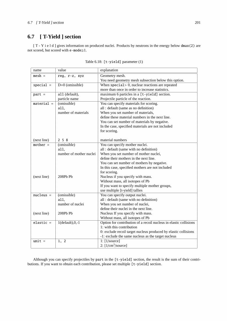
6.7 [ T-Yield ] section 201
6.7 [ T-Yield ] section
[ T - Y i e l d ] gives information on produced nuclei. Products by neutrons in the energy belowdmax(2) arenot scored, but scored withe-mode≥1.
Table 6.18:[t-yield] parameter (1)
name value explanation
mesh = reg, r-z, xyz Geometry mesh.You need geometry mesh subsection below this option.
special = D=0 (omissible) Whenspecial> 0, nuclear reactions are repeatedmore than once in order to increase statistics.
part = all (default), maximum 6 particles in a[t-yield] section.particle name Projectile particle of the reaction.
material = (omissible) You can specify materials for scoring.all, all : default (same as no definition)number of materials When you set number of materials,
define these material numbers in the next line.You can set number of materials by negative.In the case, specified materials are not includedfor scoring.
(next line) 2 5 8 material numbersmother = (omissible) You can specify mother nuclei.
all, all : default (same with no definition)number of mother nuclei When you set number of mother nuclei,
define their mothers in the next line.You can set number of mothers by negative.In this case, specified mothers are not includedfor scoring.
(next line) 208Pb Pb Nucleus if you specify with mass.Without mass, all isotopes of PbIf you want to specify multiple mother groups,use multiple [t-yield] tallies
nucleus = (omissible) You can specify output nuclei.all, all : default (same with no definition)number of nuclei When you set number of nuclei,
define their nuclei in the next line.(next line) 208Pb Pb Nucleus If you specify with mass.
Without mass, all isotopes of Pbelastic = 1(default),0,-1 Option for contribution of a recoil nucleus in elastic collisions
1: with this contribution0: exclude recoil target nucleus produced by elastic collisions-1: exclude the same nucleus as the target nucleus
unit = 1, 2 1: [1/source]2: [1/cm3/source]
Although you can specify projectiles bypart in the[t-yield] section, the result is the sum of their contri-butions. If you want to obtain each contribution, please set multiple[t-yield] section.
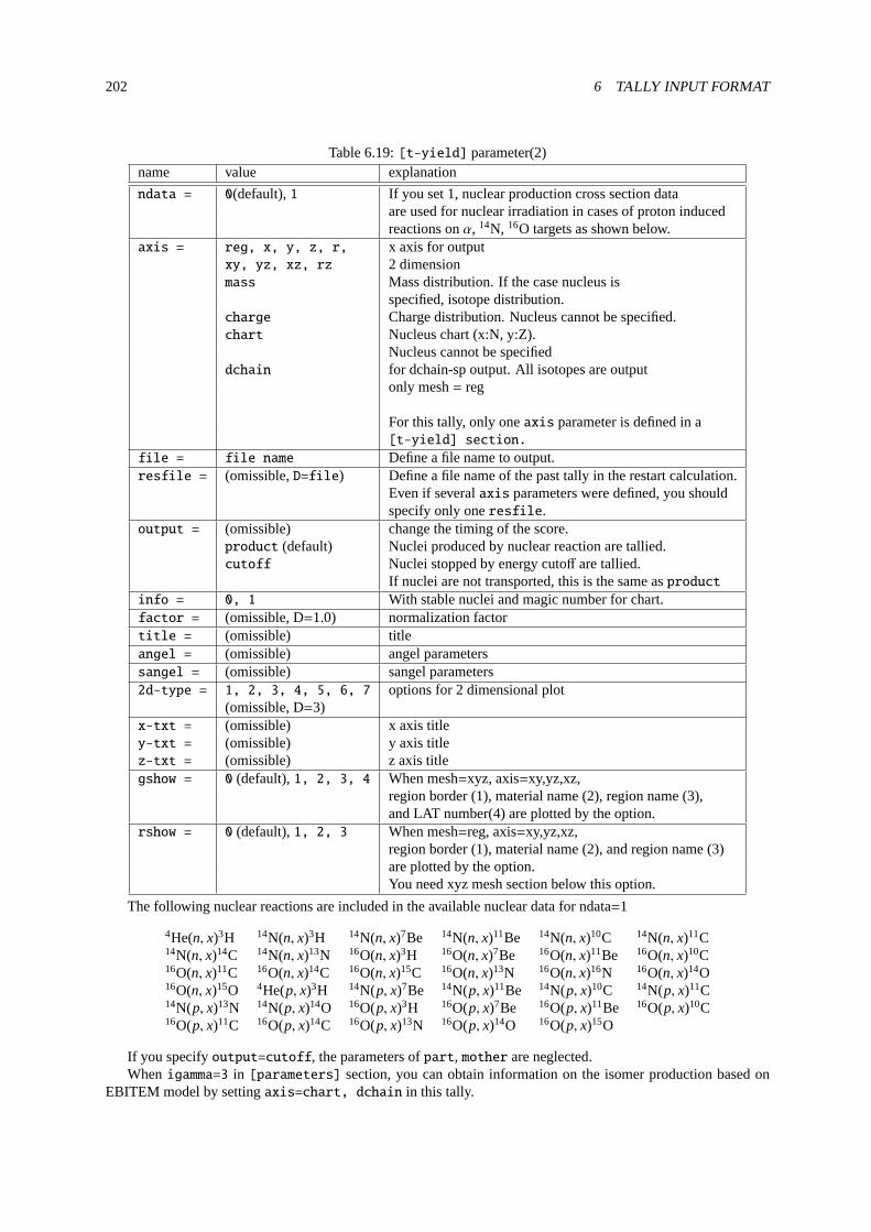
202 6 TALLY INPUT FORMAT
Table 6.19:[t-yield] parameter(2)name value explanation
ndata = 0(default),1 If you set 1, nuclear production cross section dataare used for nuclear irradiation in cases of proton inducedreactions onα, 14N, 16O targets as shown below.
axis = reg, x, y, z, r, x axis for outputxy, yz, xz, rz 2 dimensionmass Mass distribution. If the case nucleus is
specified, isotope distribution.charge Charge distribution. Nucleus cannot be specified.chart Nucleus chart (x:N, y:Z).
Nucleus cannot be specifieddchain for dchain-sp output. All isotopes are output
only mesh= reg
For this tally, only oneaxis parameter is defined in a[t-yield] section.
file = file name Define a file name to output.resfile = (omissible,D=file) Define a file name of the past tally in the restart calculation.
Even if severalaxis parameters were defined, you shouldspecify only oneresfile.
output = (omissible) change the timing of the score.product (default) Nuclei produced by nuclear reaction are tallied.cutoff Nuclei stopped by energy cutoff are tallied.
If nuclei are not transported, this is the same asproductinfo = 0, 1 With stable nuclei and magic number for chart.factor = (omissible, D=1.0) normalization factortitle = (omissible) titleangel = (omissible) angel parameterssangel = (omissible) sangel parameters2d-type = 1, 2, 3, 4, 5, 6, 7 options for 2 dimensional plot
(omissible, D=3)x-txt = (omissible) x axis titley-txt = (omissible) y axis titlez-txt = (omissible) z axis titlegshow = 0 (default),1, 2, 3, 4 When mesh=xyz, axis=xy,yz,xz,
region border (1), material name (2), region name (3),and LAT number(4) are plotted by the option.
rshow = 0 (default),1, 2, 3 When mesh=reg, axis=xy,yz,xz,region border (1), material name (2), and region name (3)are plotted by the option.You need xyz mesh section below this option.
The following nuclear reactions are included in the available nuclear data for ndata=1
4He(n, x)3H 14N(n, x)3H 14N(n, x)7Be 14N(n, x)11Be 14N(n, x)10C 14N(n, x)11C14N(n, x)14C 14N(n, x)13N 16O(n, x)3H 16O(n, x)7Be 16O(n, x)11Be 16O(n, x)10C16O(n, x)11C 16O(n, x)14C 16O(n, x)15C 16O(n, x)13N 16O(n, x)16N 16O(n, x)14O16O(n, x)15O 4He(p, x)3H 14N(p, x)7Be 14N(p, x)11Be 14N(p, x)10C 14N(p, x)11C14N(p, x)13N 14N(p, x)14O 16O(p, x)3H 16O(p, x)7Be 16O(p, x)11Be 16O(p, x)10C16O(p, x)11C 16O(p, x)14C 16O(p, x)13N 16O(p, x)14O 16O(p, x)15O
If you specifyoutput=cutoff, the parameters ofpart, mother are neglected.Whenigamma=3 in [parameters] section, you can obtain information on the isomer production based on
EBITEM model by settingaxis=chart, dchain in this tally.

6.7 [ T-Yield ] section 203
Table 6.20:[t-yield] parameter (3)
name value explanation
ginfo = 0 (default), No geometry check in the case of gshow or rshow>01 Check geometry and draw its two-dimensional view
with error information2 Check geometry, draw its two-dimensional view,
and outputting a geometry error file (.err)resol = 1 (default) The option multiplies region line resolution byresol times
with gshow or rshow option.width = 0.5 (default) The option defines the line thickness for gshow or rshow option.volume (omissible) The option defines volume for each region
for reg mesh. You need volume definitionsbelow this option.Default values are given in inputecho in the case of no definition.
reg vol volume definition. See5.1.2iechrl = 72 (default) Number of maximum column for volume input echovolmat = (omissible, D=9) The option corrects a volume value for each mesh
when material is defined by xyz mesh.(0 means no correction)Value of volmat means the number of scansfor one side of xyz mesh
epsout = 0 (default), 1, 2 Whenepsout=1, results are plotted into eps files.This eps file is named by replacing the extension into “.eps ”.Whenepsout=2, error bars are also displayed in the eps file, exceptfor axis= xy, yz, xz, rz, chart, dchain.
bmpout = 0(default), 1 Generate Bitmap figure of 2-dimensional tally output.This file is named by replacing the extension into “.bmp ”.Whenmesh=xyz, axis=(xy, yz, or xz), this is available.
vtkout = 0(default), 1 Output the tally results in xyz-mesh in the input format of ParaView.This file is named by replacing the extension into “.vtk ”.Whenmesh=xyz, axis=(xy, yz, or xz), this is available.
vtkfmt = 0(default), 1 Format of output file for ParaView.0: ascii, 1: binary.
ctmin(i) = (omissible, D=-9999) minimum value for i-th counterctmax(i) = (omissible, D= 9999) maximum value for i-th countertrcl = (omissible) coordinate transformation number or definition
for r-z or xyz meshgslat = 1(default), 0 1: show lattice boundary in gshow, 0: nostdcut = (omissible,D=-1) Threshold value of STD cut off.
By specifying output nuclei bynucleus and giving a value ofstdcut, you can automatically stop a PHITScalculation depending on values of STD (standard deviation). This function is available whenstdcut is positiveanditall=0,1 is set in[parameters] section. When all relative values of STD of the tally result are smallerthanstdcut at the last of one batch, PHITS finishes its calculation. If you setstdcut in two (or more) tallysections, all the results of the tally sections have to satisfy the conditions in order to work the function.
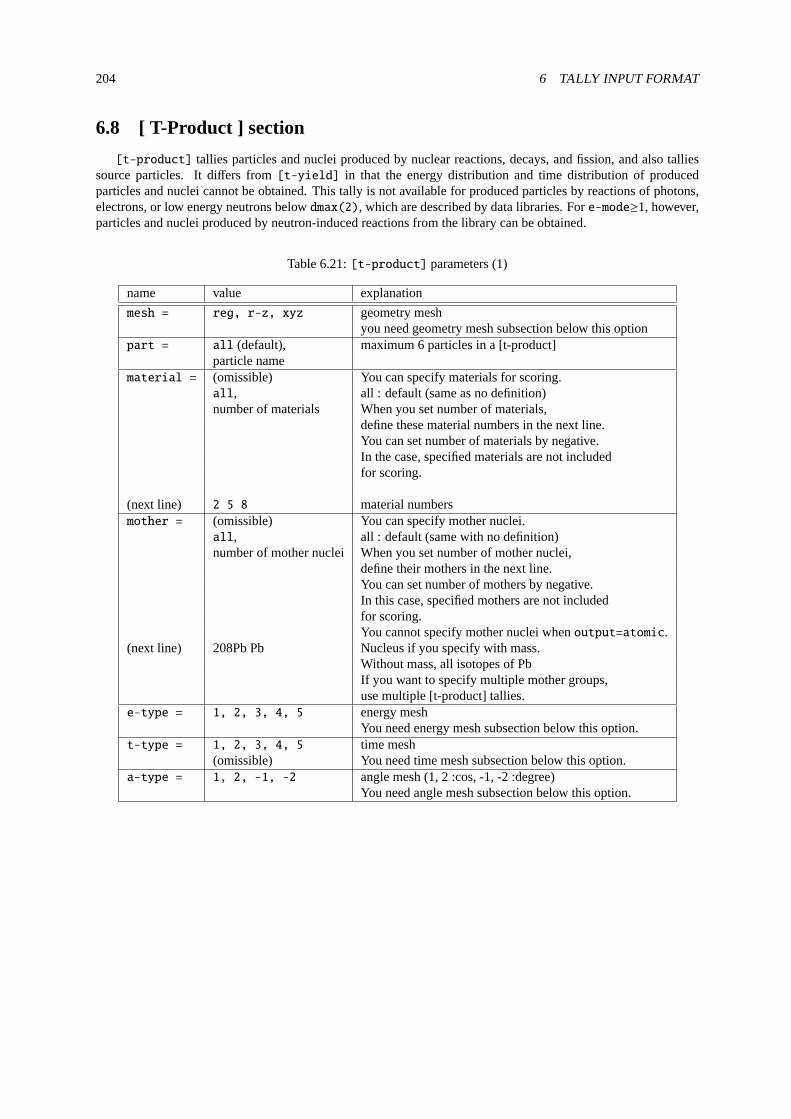
204 6 TALLY INPUT FORMAT
6.8 [ T-Product ] section
[t-product] tallies particles and nuclei produced by nuclear reactions, decays, and fission, and also talliessource particles. It differs from[t-yield] in that the energy distribution and time distribution of producedparticles and nuclei cannot be obtained. This tally is not available for produced particles by reactions of photons,electrons, or low energy neutrons belowdmax(2), which are described by data libraries. Fore-mode≥1, however,particles and nuclei produced by neutron-induced reactions from the library can be obtained.
Table 6.21:[t-product] parameters (1)
name value explanation
mesh = reg, r-z, xyz geometry meshyou need geometry mesh subsection below this option
part = all (default), maximum 6 particles in a [t-product]particle name
material = (omissible) You can specify materials for scoring.all, all : default (same as no definition)number of materials When you set number of materials,
define these material numbers in the next line.You can set number of materials by negative.In the case, specified materials are not includedfor scoring.
(next line) 2 5 8 material numbersmother = (omissible) You can specify mother nuclei.
all, all : default (same with no definition)number of mother nuclei When you set number of mother nuclei,
define their mothers in the next line.You can set number of mothers by negative.In this case, specified mothers are not includedfor scoring.You cannot specify mother nuclei whenoutput=atomic.
(next line) 208Pb Pb Nucleus if you specify with mass.Without mass, all isotopes of PbIf you want to specify multiple mother groups,use multiple [t-product] tallies.
e-type = 1, 2, 3, 4, 5 energy meshYou need energy mesh subsection below this option.
t-type = 1, 2, 3, 4, 5 time mesh(omissible) You need time mesh subsection below this option.
a-type = 1, 2, -1, -2 angle mesh (1, 2 :cos, -1, -2 :degree)You need angle mesh subsection below this option.

6.8 [ T-Product ] section 205
Table 6.22:[t-product] parameters (2)
name value explanation
unit = 1, 2, 3, 4, 5, 6 1: [1/source]2: [1/cm3/source]3: [1/MeV/source]4: [1/cm3/MeV/source]5: [1/Lethargy/source]6: [1/cm3/Lethargy/source]
11, 12, 13, 14, 15, 16 11:[1/nsec/source]12:[1/cm3/nsec/source]13:[1/MeV/nsec/source]14:[1/cm3/MeV/nsec/source]15:[1/Lethargy/nsec/source]16:[1/cm3/Lethargy/nsec/source]
21, 22, 23, 24, 25, 26 21: [1/sr/source]22: [1/cm3/sr/source]23: [1/MeV/sr/source]24: [1/cm3/MeV/sr/source]25: [1/Lethargy/sr/source]26: [1/cm3/Lethargy/sr/source]
31, 32, 33, 34, 35, 36 31:[1/nsec/sr/source]32:[1/cm3/nsec/sr/source]33:[1/MeV/nsec/sr/source]34:[1/cm3/MeV/nsec/sr/source]35:[1/Lethargy/nsec/sr/source]36:[1/cm3/Lethargy/nsec/sr/source]
“Lethargy ” in unit = 5, 6, 15, 16, 25, 26, 35 or 36 is a natural logarithmic unit of energy, anddefined by ln(Eref/E) using a reference energyEref and a particle’s energyE. If you set these units, you can obtainresults per Lethargy, which are calculated by Lethargy widths, ln(Ehigh/Elow), at each energy bins given in theenergy mesh subsection. Here,Ehigh andElow are maximum and minimum values of the energy bins, respectively.
“sr ” in unit = 21 - 26 or 31 - 36 denotes steradian, unit of solid angle.
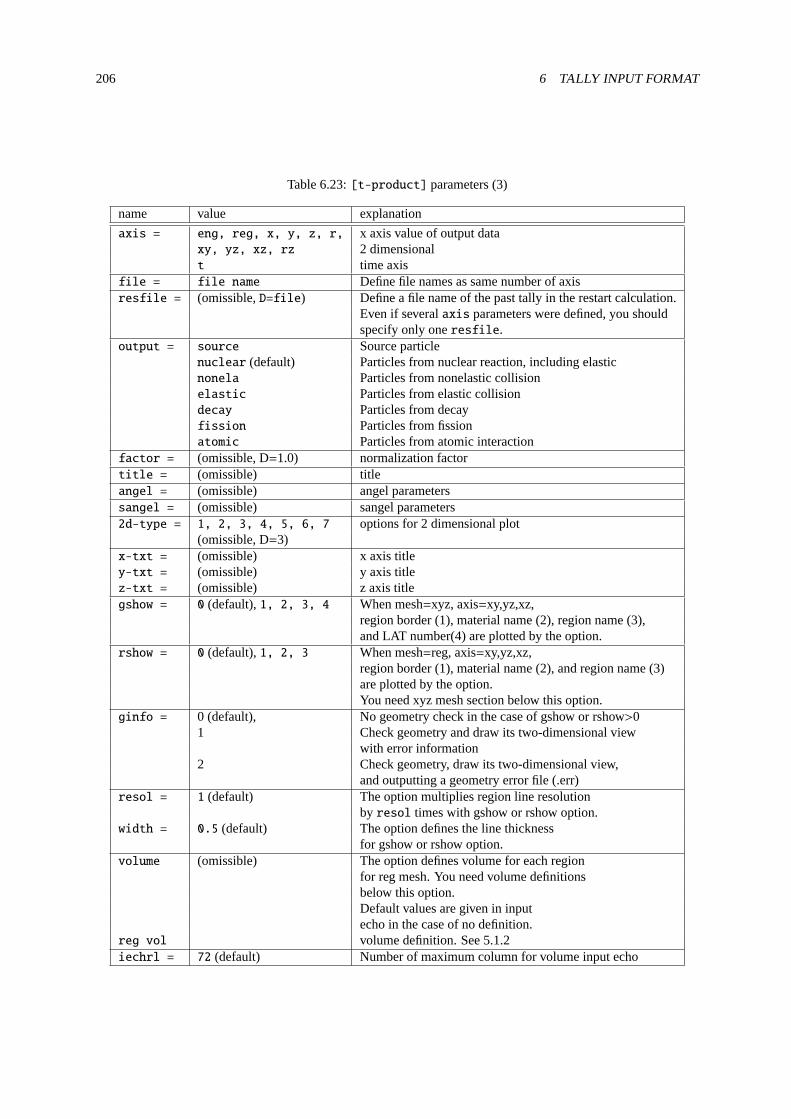
206 6 TALLY INPUT FORMAT
Table 6.23:[t-product] parameters (3)
name value explanation
axis = eng, reg, x, y, z, r, x axis value of output dataxy, yz, xz, rz 2 dimensionalt time axis
file = file name Define file names as same number of axisresfile = (omissible,D=file) Define a file name of the past tally in the restart calculation.
Even if severalaxis parameters were defined, you shouldspecify only oneresfile.
output = source Source particlenuclear (default) Particles from nuclear reaction, including elasticnonela Particles from nonelastic collisionelastic Particles from elastic collisiondecay Particles from decayfission Particles from fissionatomic Particles from atomic interaction
factor = (omissible, D=1.0) normalization factortitle = (omissible) titleangel = (omissible) angel parameterssangel = (omissible) sangel parameters2d-type = 1, 2, 3, 4, 5, 6, 7 options for 2 dimensional plot
(omissible, D=3)x-txt = (omissible) x axis titley-txt = (omissible) y axis titlez-txt = (omissible) z axis titlegshow = 0 (default),1, 2, 3, 4 When mesh=xyz, axis=xy,yz,xz,
region border (1), material name (2), region name (3),and LAT number(4) are plotted by the option.
rshow = 0 (default),1, 2, 3 When mesh=reg, axis=xy,yz,xz,region border (1), material name (2), and region name (3)are plotted by the option.You need xyz mesh section below this option.
ginfo = 0 (default), No geometry check in the case of gshow or rshow>01 Check geometry and draw its two-dimensional view
with error information2 Check geometry, draw its two-dimensional view,
and outputting a geometry error file (.err)resol = 1 (default) The option multiplies region line resolution
by resol times with gshow or rshow option.width = 0.5 (default) The option defines the line thickness
for gshow or rshow option.volume (omissible) The option defines volume for each region
for reg mesh. You need volume definitionsbelow this option.Default values are given in inputecho in the case of no definition.
reg vol volume definition. See5.1.2iechrl = 72 (default) Number of maximum column for volume input echo
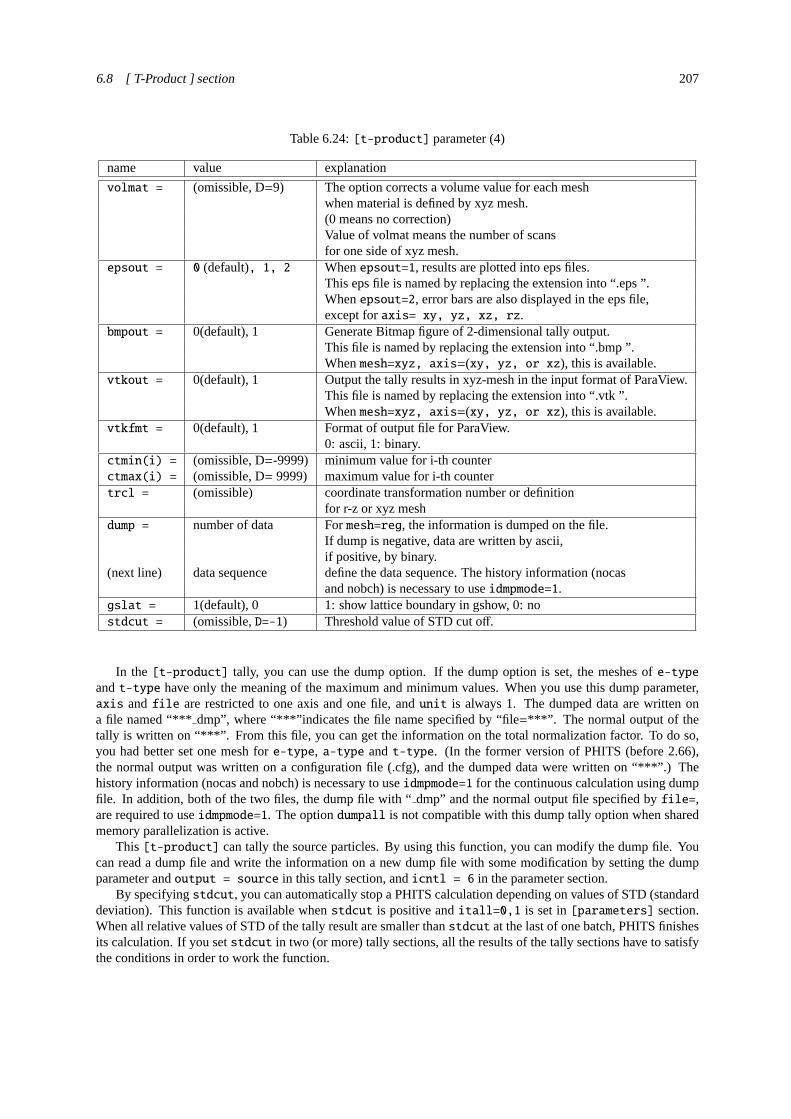
6.8 [ T-Product ] section 207
Table 6.24:[t-product] parameter (4)
name value explanation
volmat = (omissible, D=9) The option corrects a volume value for each meshwhen material is defined by xyz mesh.(0 means no correction)Value of volmat means the number of scansfor one side of xyz mesh.
epsout = 0 (default), 1, 2 Whenepsout=1, results are plotted into eps files.This eps file is named by replacing the extension into “.eps ”.Whenepsout=2, error bars are also displayed in the eps file,except foraxis= xy, yz, xz, rz.
bmpout = 0(default), 1 Generate Bitmap figure of 2-dimensional tally output.This file is named by replacing the extension into “.bmp ”.Whenmesh=xyz, axis=(xy, yz, or xz), this is available.
vtkout = 0(default), 1 Output the tally results in xyz-mesh in the input format of ParaView.This file is named by replacing the extension into “.vtk ”.Whenmesh=xyz, axis=(xy, yz, or xz), this is available.
vtkfmt = 0(default), 1 Format of output file for ParaView.0: ascii, 1: binary.
ctmin(i) = (omissible, D=-9999) minimum value for i-th counterctmax(i) = (omissible, D= 9999) maximum value for i-th countertrcl = (omissible) coordinate transformation number or definition
for r-z or xyz meshdump = number of data Formesh=reg, the information is dumped on the file.
If dump is negative, data are written by ascii,if positive, by binary.
(next line) data sequence define the data sequence. The history information (nocasand nobch) is necessary to useidmpmode=1.
gslat = 1(default), 0 1: show lattice boundary in gshow, 0: nostdcut = (omissible,D=-1) Threshold value of STD cut off.
In the [t-product] tally, you can use the dump option. If the dump option is set, the meshes ofe-type
andt-type have only the meaning of the maximum and minimum values. When you use this dump parameter,axis andfile are restricted to one axis and one file, andunit is always 1. The dumped data are written ona file named “*** dmp”, where “***”indicates the file name specified by “file=***”. The normal output of thetally is written on “***”. From this file, you can get the information on the total normalization factor. To do so,you had better set one mesh fore-type, a-type andt-type. (In the former version of PHITS (before 2.66),the normal output was written on a configuration file (.cfg), and the dumped data were written on “***”.) Thehistory information (nocas and nobch) is necessary to useidmpmode=1 for the continuous calculation using dumpfile. In addition, both of the two files, the dump file with “dmp” and the normal output file specified byfile=,are required to useidmpmode=1. The optiondumpall is not compatible with this dump tally option when sharedmemory parallelization is active.
This [t-product] can tally the source particles. By using this function, you can modify the dump file. Youcan read a dump file and write the information on a new dump file with some modification by setting the dumpparameter andoutput = source in this tally section, andicntl = 6 in the parameter section.
By specifyingstdcut, you can automatically stop a PHITS calculation depending on values of STD (standarddeviation). This function is available whenstdcut is positive anditall=0,1 is set in[parameters] section.When all relative values of STD of the tally result are smaller thanstdcut at the last of one batch, PHITS finishesits calculation. If you setstdcut in two (or more) tally sections, all the results of the tally sections have to satisfythe conditions in order to work the function.

208 6 TALLY INPUT FORMAT
6.9 [ T-DPA ] section
[ T - D P A ] gives DPA (Displacement Per Atom) value. This is the number of displaced atoms per a targetatom, and represents the radiation damage in materials irradiated by energetic particles. The result by this tallyincludes the contribution of Coulomb scattering cross section for the charged particle transportation. DPA by lowenergy neutron incident reactions can be also obtained by usinge-mode≥1.
Table 6.25:[t-dpa] parameter (1)
name value explanation
mesh = reg, r-z, xyz geometry meshyou need geometry mesh subsection below this option
part = all (default), maximum 6 particles in a [t-dpa]particle name
material = (omissible) You can specify materials for scoring.all, all : default (same as no definition)number of materials When you set number of materials,
define these material numbers in the next line.You can set number of materials by negative.In the case, specified materials are not includedfor scoring.
(next line) 2 5 8 material numbersmother = (omissible) You can specify mother nuclei.
all, all : default (same with no definition)number of mother nuclei When you set number of mother nuclei,
define their mothers in the next line.You can set number of mothers by negative.In this case, specified mothers are not includedfor scoring.
(next line) 208Pb Pb Nucleus if you specify with mass.Without mass, all isotopes of Pb.If you want to specify multiple mother groups,use multiple [t-dpa] tallies.
unit = 1, 2 1: [DPA*1.e-24/source]2: [DPA/source]
axis = eng, reg, x, y, z, r, x axis value of output dataxy, yz, xz, rz 2 dimensional
file = file name Define file names as same number of axisresfile = (omissible,D=file) Define a file name of the past tally in the restart calculation.
Even if severalaxis parameters were defined, you shouldspecify only oneresfile.

6.9 [ T-DPA ] section 209
Table 6.26:[t-dpa] parameter (2)
name value explanation
output = dpa total: total DPA valuecutoff1: DPA value when energies of charged particlesproduced by reactions are below cutoff energy (emin)cutoff2: DPA value when energies of charged particlestransported in materials are below cutoff energy (emin)transpt: DPA value when charged particles are transported
all add d, t,3He,α, and nucleus contributions as PKA,with “simple”
factor = (omissible, D=1.0) normalization factortitle = (omissible) titleangel = (omissible) angel parameterssangel = (omissible) sangel parameters2d-type = 1, 2, 3, 4, 5, 6, 7 options for 2 dimensional plot
(omissible, D=3)x-txt = (omissible) x axis titley-txt = (omissible) y axis titlez-txt = (omissible) z axis titlegshow = 0 (default),1, 2, 3, 4 When mesh=xyz, axis=xy,yz,xz,
region border (1), material name (2), region name (3),and LAT number(4) are plotted by the option.
rshow = 0 (default),1, 2, 3 When mesh=reg, axis=xy,yz,xz,region border (1), material name (2), and region name (3)are plotted by the option.You need xyz mesh section below this option.
ginfo = 0 (default), No geometry check in the case of gshow or rshow>01 Check geometry and draw its two-dimensional view
with error information2 Check geometry, draw its two-dimensional view,
and outputting a geometry error file (.err)resol = 1 (default) The option multiplies region line resolution
by resol times with gshow or rshow option.width = 0.5 (default) The option defines the line thickness
for gshow or rshow option.volume (omissible) The option defines volume for each region
for reg mesh. You need volume definitionsbelow this option.Default values are given in inputecho in the case of no definition.
reg vol volume definition. See5.1.2iechrl = 72 (default) Number of maximum column for volume input echovolmat = (omissible, D=9) The option corrects a volume value for each mesh
when material is defined by xyz mesh.(0 means no correction)Value of volmat means the number of scansfor one side of xyz mesh.

210 6 TALLY INPUT FORMAT
Table 6.27:[t-dpa] parameter (3)
name value explanation
epsout = 0 (default), 1, 2 Whenepsout=1, results are plotted into eps files.This eps file is named by replacing the extension into “.eps ”.Whenepsout=2, error bars are also displayed in the eps file,except foraxis= xy, yz, xz, rz.
bmpout = 0(default), 1 Generate Bitmap figure of 2-dimensional tally output.This file is named by replacing the extension into “.bmp ”.Whenmesh=xyz, axis=(xy, yz, or xz), this is available.
vtkout = 0(default), 1 Output the tally results in xyz-mesh in the input format of ParaView.This file is named by replacing the extension into “.vtk ”.Whenmesh=xyz, axis=(xy, yz, or xz), this is available.
vtkfmt = 0(default), 1 Format of output file for ParaView.0: ascii, 1: binary.
ctmin(i) = (omissible, D=-9999) minimum value for i-th counterctmax(i) = (omissible, D= 9999) maximum value for i-th countertrcl = (omissible) coordinate transformation number or definition
for r-z or xyz meshgslat = 1(default), 0 1: show lattice boundary in gshow, 0: nostdcut = (omissible,D=-1) Threshold value of STD cut off.
By specifyingstdcut, you can automatically stop a PHITS calculation depending on values of STD (standarddeviation). This function is available whenstdcut is positive anditall=0,1 is set in[parameters] section.When all relative values of STD of the tally result are smaller thanstdcut at the last of one batch, PHITS finishesits calculation. If you setstdcut in two (or more) tally sections, all the results of the tally sections have to satisfythe conditions in order to work the function.

6.10 [ T-LET ] section 211
6.10 [ T-LET ] section
By the LET tally, you can get the information on track length and dose as a function of LET(dE/dx) of acertain material. This tally counts an energy loss of charged particles and nuclei, and thus, you must use the EventGenerator mode (e-mode≥1) if you would like to transport low-energy neutrons. Note that this tally does notconsider the contribution of the electron and positron below their cutoff energy (emin) to the result.
Table 6.28:[t-let] parameters(1)
name value explanation
mesh = reg, r-z, xyz geometry meshyou need geometry mesh subsection below this option
part = all (default), maximum 6 particles in a [t-let]particle name
material = (omissible) You can specify materials for scoring.all, all : default (same as no definition)number of materials When you set number of materials,
define these material numbers in the next line.You can set number of materials by negative.In the case, specified materials are not includedfor scoring.
(next line) 2 5 8 material numbersletmat = (omissible) material id for LET(dE/dx).
If omitted, real material is assumed.If you select the material that is not used in your geometry,you have to define its material density in [material] section.If you would like to calculate LET in water, you have todefine water with 1 g/cm3 in [material] sectiont.When you set letmat< 0, PHITS automatically calculatesdE/dx for water with 1 g/cm3 for electrons and positrons.Please see “particletherapy” in the recommendation settingin more detail.
l-type = 1, 2, 3, 4, 5 LET meshYou need LET mesh subsection below this optionIt is noted that the LET spectrum may have unnatural peakswhen you set a very fine mesh, e.g., 20 meshes per oneorder of magnitude.

212 6 TALLY INPUT FORMAT
Table 6.29:[t-let] parameter (2)
name value explanation
unit = 1, 2, 3, 4, 5, 6 1: Track [cm/(keV/µm)/source]2: Dose [MeV/(keV/µm)/source]3: Track [cm/ln(keV/µm)/source]4: Dose [MeV/ln(keV/µm)/source]5: Track [cm/source]6: Dose [MeV/source]
7, 8, 9, 10, 11, 12 7: Track [1/cm2/(keV/µm)/source]8: Dose [MeV/cm3/(keV/µm)/source]9: Track [1/cm2/ln(keV/µm)/source]10:Dose [MeV/cm3/ln(keV/µm)/source]11:Track [1/cm2/source]12:Dose [MeV/cm3/source]
13, 14 13: L ∗ f (L) [dimensionless], where∫
f (L)dL = 1.14: L ∗ d(L) [keV/µm], where
∫d(L)dL = 1.
axis = let, reg, x, y, z, r, x axis value of output dataxy, yz, xz, rz 2 dimensional
file = file name Define file names as same number of axisresfile = (omissible,D=file) Define a file name of the past tally in the restart calculation.
Even if severalaxis parameters were defined, you shouldspecify only oneresfile.
factor = (omissible, D=1.0) normalization factortitle = (omissible) titleangel = (omissible) angel parameterssangel = (omissible) sangel parameters2d-type = 1, 2, 3, 4, 5, 6, 7 options for 2 dimensional plot
(omissible, D=3)x-txt = (omissible) x axis titley-txt = (omissible) y axis titlez-txt = (omissible) z axis title
From version 3.02, new options (unit=13 and14) were implemented. Using them, the frequency and doseprobability densities of LETL, f (L) andd(L), respectively, can be easily calculated. The results obtained fromunit=13 and14 are proportional to those obtained fromunit=2 and4, respectively, but their absolute valuesare different because the integral of the probability densities are normalized to 1 for the new options. Note thatunit=13 and14 can be set only whenaxis=let.

6.10 [ T-LET ] section 213
Table 6.30:[t-let] parameter (3)
name value explanation
gshow = 0 (default),1, 2, 3, 4 When mesh=xyz, axis=xy,yz,xz,region border (1), material name (2), region name (3),and LAT number(4) are plotted by the option.
rshow = 0 (default),1, 2, 3 When mesh=reg, axis=xy,yz,xz,region border (1), material name (2), and region name (3)are plotted by the option.You need xyz mesh section below this option.
ginfo = 0 (default), No geometry check in the case of gshow or rshow>01 Check geometry and draw its two-dimensional view
with error information2 Check geometry, draw its two-dimensional view,
and outputting a geometry error file (.err)resol = 1 (default) The option multiplies region line resolution
by resol times with gshow or rshow option.width = 0.5 (default) The option defines the line thickness
for gshow or rshow option.volume (omissible) The option defines volume for each region
for reg mesh. You need volume definitionsbelow this option.Default values are given in inputecho in the case of no definition.
reg vol volume definition. See5.1.2iechrl = 72 (default) Number of maximum column for volume input echovolmat = (omissible, D=9) The option corrects a volume value for each mesh
when material is defined by xyz mesh.(0 means no correction)Value of volmat means the number of scansfor one side of xyz mesh.
epsout = 0 (default), 1, 2 Whenepsout=1, results are plotted into eps files.This eps file is named by replacing the extension into “.eps ”.Whenepsout=2, error bars are also displayed in the eps file,except foraxis= xy, yz, xz, rz.
ctmin(i) = (omissible, D=-9999) minimum value for i-th counterctmax(i) = (omissible, D= 9999) maximum value for i-th countertrcl = (omissible) coordinate transformation number or definition
for r-z or xyz meshgslat = 1(default), 0 1: show lattice boundary in gshow, 0: nostdcut = (omissible,D=-1) Threshold value of STD cut off.
By specifyingstdcut, you can automatically stop a PHITS calculation depending on values of STD (standarddeviation). This function is available whenstdcut is positive anditall=0,1 is set in[parameters] section.When all relative values of STD of the tally result are smaller thanstdcut at the last of one batch, PHITS finishesits calculation. If you setstdcut in two (or more) tally sections, all the results of the tally sections have to satisfythe conditions in order to work the function.

214 6 TALLY INPUT FORMAT
6.11 [ T-SED ] section
Calculation of the probability density of deposition energies in microscopic sites, called as lineal energyyor specific energyz, is of great importance in estimation of relative biological effectiveness (RBE) of chargedparticles. However, such microscopic probability densities cannot be directly calculated by PHITS simulationusing[t-deposit] or [t-heat] tallies, since PHITS is designed to simulate particle motions in macroscopicscale, and employs a continuous-slowing-down approximation (CSDA) for calculating the energy loss of chargedparticles. We therefore introduced a special tally named[t-sed] for calculating the microscopic probabilitydensities using a mathematical function that can instantaneously calculate quantities around trajectories of chargedparticles. The function was developed on the basis of track structure simulation, considering productions ofδ-raysand Auger electrons. Note that the name of “SED” derives from “Specific Energy Distribution”. Details of thecalculation procedure are given elsewhere.49 50 The function of[delta ray] section shouldn’t be used togetherwith this tally.
Using this tally, we can get information on probability densities ofy andz in water. We can also calculate theprobability densities in different materials, although the accuracy has not been checked yet. Similar to[t-let],the dose is only counted in an energy loss of charged particles and nuclei, and thus, we must use the event generatormode (e-mode≥1) if we would like to transport low-energy neutrons. The deposition energy in microscopic sitescan be expressed by deposit energyε in MeV, lineal energy y in keV/µm or specific energyz in Gy. The definitionsof these quantities are given in ICRU Report 36. Usage of[t-sed] is similar to that of[t-let].
Table 6.31:[t-sed] parameters (1)
name value explanation
mesh = reg, r-z, xyz geometry meshyou need geometry mesh subsection below this option
part = all (default), maximum 6 particles in a [t-sed]particle name
material = (omissible) You can specify materials for scoring.all, all : default (same as no definition)number of materials When you set number of materials,
define these material numbers in the next line.You can set number of materials by negative.In the case, specified materials are not includedfor scoring.
(next line) 2 5 8 material numbersletmat = (omissible) material id for LET(dE/dx).
If omitted, real material is assumed.If you select the material that is not used in your geometry,you have to define its material density in [material] section.If you would like to calculate LET in water, you have todefine water with 1 g/cm3 in [material] sectiont.When you set letmat< 0, PHITS automatically calculatesdE/dx for water with 1 g/cm3 for electrons and positrons.Please see “particletherapy” in the recommendation settingin more detail.
se-unit = 1, 2, 3 Unit of deposition energy in microscopic site1: deposit energyε in MeV2: lineal energyy in keV/µm3: specific energyz in Gy
cdiam = (omissible, D=1.0) Diameter of the microscopic site inµm.You can select the value from 0.001 to 2.0.
49 T. Sato, R. Watanabe and K. Niita,“ Development of a calculation method for estimating the specific energy distribution in complexradiation fields”, Radiat. Prot. Dosim. 122, 41-45 (2006).
50 T. Sato, Y. Kase, R. Watanabe, K. Niita and L. Sihver,“Biological dose estimation for charged-particle therapy using an improved PHITScode coupled with a microdosimetric kinetic model”, Radiat. Res. 171, 107-117 (2009).

6.11 [ T-SED ] section 215
Table 6.32:[t-sed] parameters (2)
name value explanation
se-type = 1, 2, 3, 4, 5 ε, y or z mesh (unit is defined byse-unit):an energy mesh subsection (specified inne, emin, emax, etc.)is required below this option. If a “Warning: Z bin is notenough!” message occurs, theemin, emax, andne parametersmust be changed. This warning indicates that the microdosimet-ric function cannot calculate they (or z) distribution because therange is too small or the mesh resolution is too poor. For exam-ple, setse-type=3, emin=0.01, emax=10000.0, ne=60 orhigher for calculating they distribution for cite diameter= 1 µm(cdiam=1.0, se-unit=2).
unit = 1, 2, 3, 4, 5, 6 1: Track [cm/(keV/µm)/source]2: Dose [MeV/(keV/µm)/source], proportional toy ∗ f (y).3: Track [cm/ln(keV/µm)/source]4: Dose [MeV/ln(keV/µm)/source], proportional toy ∗ d(y).5: Track [cm/source]6: Dose [MeV/source]
7,8 7: y ∗ f (y) [dimensionless], where∫
f (y)dy= 1.8: y ∗ d(y) [keV/µm], where
∫d(y)dy= 1.
These units are for the case ofse-unit=2. Forse-unit=1 and3, (keV/µm) is replaced by (MeV) and (Gy), respectively.
axis = sed, reg, x, y, z, r, x axis value of output dataxy, yz, xz, rz 2 dimensional
file = file name Define file names as same number of axisresfile = (omissible,D=file) Define a file name of the past tally in the restart calculation.
Even if severalaxis parameters were defined, you should specifyonly oneresfile.
factor = (omissible, D=1.0) normalization factortitle = (omissible) titleangel = (omissible) angel parameterssangel = (omissible) sangel parameters2d-type = 1, 2, 3, 4, 5, 6, 7 options for 2 dimensional plot
(omissible, D=3)x-txt = (omissible) x axis titley-txt = (omissible) y axis titlez-txt = (omissible) z axis title
From version 3.02, new options (unit=7 and8) were implemented. Using them, the frequency and doseprobability densities ofy, f (y) andd(y), respectively, can be easily calculated. The results obtained fromunit=7
and8 are proportional to those obtained fromunit=2 and4, respectively, but their absolute values are differentbecause the integral of the probability densities are normalized to 1 in the cases of the new options. Note thatunit=13 and14 can be set only whenaxis=sed.

216 6 TALLY INPUT FORMAT
Table 6.33:[t-sed] parameters (3)
name value explanation
gshow = 0 (default),1, 2, 3, 4 When mesh=xyz, axis=xy,yz,xz,region border (1), material name (2), region name (3),and LAT number(4) are plotted by the option.
rshow = 0 (default),1, 2, 3 When mesh=reg, axis=xy,yz,xz,region border (1), material name (2), and region name (3)are plotted by the option.You need xyz mesh section below this option.
ginfo = 0 (default), No geometry check in the case of gshow or rshow>01 Check geometry and draw its two-dimensional view
with error information2 Check geometry, draw its two-dimensional view,
and outputting a geometry error file (.err)resol = 1 (default) The option multiplies region line resolution
by resol times with gshow or rshow option.width = 0.5 (default) The option defines the line thickness
for gshow or rshow option.volume (omissible) The option defines volume for each region
for reg mesh. You need volume definitionsbelow this option.Default values are given in inputecho in the case of no definition.
reg vol volume definition. See5.1.2iechrl = 72 (default) Number of maximum column for volume input echovolmat = (omissible, D=9) The option corrects a volume value for each mesh
when material is defined by xyz mesh.(0 means no correction)Value of volmat means the number of scansfor one side of xyz mesh.
epsout = 0 (default), 1, 2 Whenepsout=1, results are plotted into eps files.This eps file is named by replacing the extension into “.eps ”.Whenepsout=2, error bars are also displayed in the eps file,except foraxis= xy, yz, xz, rz.
ctmin(i) = (omissible, D=-9999) minimum value for i-th counterctmax(i) = (omissible, D= 9999) maximum value for i-th countertrcl = (omissible) coordinate transformation number or definition
for r-z or xyz meshgslat = 1(default), 0 1: show lattice boundary in gshow, 0: nostdcut = (omissible,D=-1) Threshold value of STD cut off.
By specifyingstdcut, you can automatically stop a PHITS calculation depending on values of STD (standarddeviation). This function is available whenstdcut is positive anditall=0,1 is set in[parameters] section.When all relative values of STD of the tally result are smaller thanstdcut at the last of one batch, PHITS finishesits calculation. If you setstdcut in two (or more) tally sections, all the results of the tally sections have to satisfythe conditions in order to work the function.
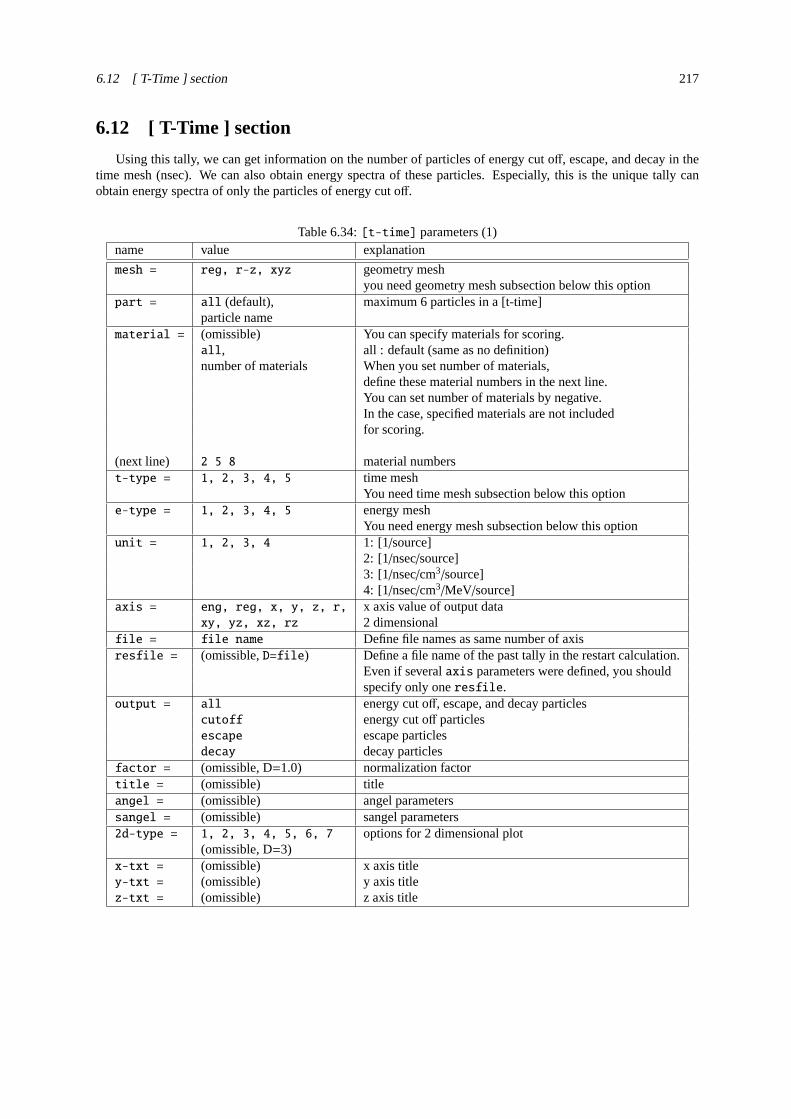
6.12 [ T-Time ] section 217
6.12 [ T-Time ] section
Using this tally, we can get information on the number of particles of energy cut off, escape, and decay in thetime mesh (nsec). We can also obtain energy spectra of these particles. Especially, this is the unique tally canobtain energy spectra of only the particles of energy cut off.
Table 6.34:[t-time] parameters (1)name value explanation
mesh = reg, r-z, xyz geometry meshyou need geometry mesh subsection below this option
part = all (default), maximum 6 particles in a [t-time]particle name
material = (omissible) You can specify materials for scoring.all, all : default (same as no definition)number of materials When you set number of materials,
define these material numbers in the next line.You can set number of materials by negative.In the case, specified materials are not includedfor scoring.
(next line) 2 5 8 material numberst-type = 1, 2, 3, 4, 5 time mesh
You need time mesh subsection below this optione-type = 1, 2, 3, 4, 5 energy mesh
You need energy mesh subsection below this optionunit = 1, 2, 3, 4 1: [1/source]
2: [1/nsec/source]3: [1/nsec/cm3/source]4: [1/nsec/cm3/MeV/source]
axis = eng, reg, x, y, z, r, x axis value of output dataxy, yz, xz, rz 2 dimensional
file = file name Define file names as same number of axisresfile = (omissible,D=file) Define a file name of the past tally in the restart calculation.
Even if severalaxis parameters were defined, you shouldspecify only oneresfile.
output = all energy cut off, escape, and decay particlescutoff energy cut off particlesescape escape particlesdecay decay particles
factor = (omissible, D=1.0) normalization factortitle = (omissible) titleangel = (omissible) angel parameterssangel = (omissible) sangel parameters2d-type = 1, 2, 3, 4, 5, 6, 7 options for 2 dimensional plot
(omissible, D=3)x-txt = (omissible) x axis titley-txt = (omissible) y axis titlez-txt = (omissible) z axis title

218 6 TALLY INPUT FORMAT
Table 6.35:[t-time] parameter (2)
name value explanation
gshow = 0 (default),1, 2, 3, 4 When mesh=xyz, axis=xy,yz,xz,region border (1), material name (2), region name (3),and LAT number(4) are plotted by the option.
rshow = 0 (default),1, 2, 3 When mesh=reg, axis=xy,yz,xz,region border (1), material name (2), and region name (3)are plotted by the option.You need xyz mesh section below this option.
ginfo = 0 (default), No geometry check in the case of gshow or rshow>01 Check geometry and draw its two-dimensional view
with error information2 Check geometry, draw its two-dimensional view,
and outputting a geometry error file (.err)resol = 1 (default) The option multiplies region line resolution
by resol times with gshow or rshow option.width = 0.5 (default) The option defines the line thickness
for gshow or rshow option.volume (omissible) The option defines volume for each region
for reg mesh. You need volume definitionsbelow this option.Default values are given in inputecho in the case of no definition.
reg vol volume definition. See5.1.2iechrl = 72 (default) Number of maximum column for volume input echovolmat = (omissible, D=9) The option corrects a volume value for each mesh
when material is defined by xyz mesh.(0 means no correction)Value of volmat means the number of scansfor one side of xyz mesh
epsout = 0 (default), 1, 2 Whenepsout=1, results are plotted into eps files.This eps file is named by replacing the extension into “.eps ”.Whenepsout=2, error bars are also displayed in the eps file,except foraxis= xy, yz, xz, rz.
bmpout = 0(default), 1 Generate Bitmap figure of 2-dimensional tally output.This file is named by replacing the extension into “.bmp ”.Whenmesh=xyz, axis=(xy, yz, or xz), this is available.
vtkout = 0(default), 1 Output the tally results in xyz-mesh in the input format of ParaView.This file is named by replacing the extension into “.vtk ”.Whenmesh=xyz, axis=(xy, yz, or xz), this is available.
vtkfmt = 0(default), 1 Format of output file for ParaView.0: ascii, 1: binary.
ctmin(i) = (omissible, D=-9999) minimum value for i-th counterctmax(i) = (omissible, D= 9999) maximum value for i-th countertrcl = (omissible) coordinate transformation number or definition
for r-z or xyz mesh

6.12 [ T-Time ] section 219
Table 6.36:[t-time] parameter (3)
name value explanation
dump = number of data Formesh=reg, the information is dumped on the file.If dump is negative, data is written by ascii,if positive, by binary.
(next line) data sequence define the data sequence. The history information (nocasand nobch) is necessary to useidmpmode=1.
gslat = 1(default), 0 1: show lattice boundary in gshow, 0: nostdcut = (omissible,D=-1) Threshold value of STD cut off.
In [t-time] tally, you can use the dump option only withoutput = cutoff. If the dump option is set, themeshes ofe-type andt-type have only the meaning of the maximum and minimum values, and unit is set tobe 1. When you use this dump parameter,axis andfile are restricted to one axis and one file, andunit isalways 1. The dumped data are written on a file named “***dmp”, where “***”indicates the file name specifiedby “file=***”. The normal output of the tally is written on “***”. From this file, you can get the informationon the total normalization factor. To do so, you had better set one mesh fore-type, a-type andt-type. (Inthe former version of PHITS (before 2.66), the normal output was written on a configuration file (.cfg), and thedumped data were written on “***”.) The history information (nocas and nobch) is necessary to useidmpmode=1
for the continuous calculation using dump file. In addition, both of the two files, the dump file with “dmp” andthe normal output file specified byfile=, are required to useidmpmode=1. The optiondumpall is not compatiblewith this dump tally option when shared memory parallelization is active.
By this dump option, you can create similar files to ncut, gcut and pcut files for the sequential calculations ofthe other transport code.
By specifyingstdcut, you can automatically stop a PHITS calculation depending on values of STD (standarddeviation). This function is available whenstdcut is positive anditall=0,1 is set in[parameters] section.When all relative values of STD of the tally result are smaller thanstdcut at the last of one batch, PHITS finishesits calculation. If you setstdcut in two (or more) tally sections, all the results of the tally sections have to satisfythe conditions in order to work the function.

220 6 TALLY INPUT FORMAT
6.13 [ T-Star ] section
This tally gives the number that nuclear reactions occur. When nuclear data libraries are used, only neutronsare tallied.
You must use the EGS5 mode if you whould like to calculate star density of atomic interactions.
Table 6.37:[t-star] parameter (1)
name value explanation
mesh = reg, r-z, xyz geometry meshyou need geometry mesh subsection below this option
part = all (default), maximum 6 particles in a [t-star]particle name projectile particle of the reaction
material = (omissible) You can specify materials for scoring.all, all : default (same as no definition)number of materials When you set number of materials,
define these material numbers in the next line.You can set number of materials by negative.In the case, specified materials are not includedfor scoring.
(next line) 2 5 8 material numbersmother = (omissible) You can specify mother nuclei.
all, all : default (same with no definition)number of mother nuclei When you set number of mother nuclei,
define their mothers in the next line.You can set number of mothers by negative.In this case, specified mothers are not includedfor scoring.You cannot specify mother nuclei whenoutput=atomic.
(next line) 208Pb Pb Nucleus if you specify with mass.Without mass, all isotopes of Pb.If you want to specify multiple mother groups,use multiple [t-star] tallies
nucleus = (omissible) You can specify output nuclei.all, all : default (same with no definition)number of nuclei When you set number of nuclei,
define their nuclei in the next line.(next line) 208Pb Pb Nucleus if you specify with mass.
Without mass, all isotopes of Pb.e-type = 1, 2, 3, 4, 5 energy mesh
You need energy mesh subsection below this option.t-type = 1, 2, 3, 4, 5 time mesh
(omissible) You need time mesh subsection below this optionunit = 1, 2 1: [1/cm3/source]
2: [1/cm3/MeV/source]axis = eng, reg, x, y, z, r, x axis value of output data
xy, yz, xz, rz 2 dimensional

6.13 [ T-Star ] section 221
Table 6.38:[t-star] parameter (2)
name value explanation
file = file name Define file names as same number of axis.resfile = (omissible,D=file) Define a file name of the past tally in the restart calculation.
Even if severalaxis parameters were defined, you shouldspecify only oneresfile.
output = all star density for all reactionsdecay star density for decay reactionelastic star density for elastic reactionnuclear star density for non-elastic+ Hydrogen+ HIfission star density for fissionabsorption star density for absorptionheavyion star density for Heavy Ion reactiontransmut star density for a reaction which induces transmutation
of target nucleusatomic star densify for atomic interaction excluding multiple scatteringdeltaray star densify for delta-ray productionatmflu star densify for atomic fluorescence x-ray emissionauger star densify for generating auger electron emissionbrems star densify for bremsstrahlungphotoelec star densify for photoelectric effectcompton star densify for compton scatteringpairprod star densify for electron-positron pair productionannih star densify for positron annihilation
factor = (omissible, D=1.0) normalization factortitle = (omissible) titleangel = (omissible) angel parameterssangel = (omissible) sangel parameters2d-type = 1, 2, 3, 4, 5, 6, 7 options for 2 dimensional plot
(omissible, D=3)x-txt = (omissible) x axis titley-txt = (omissible) y axis titlez-txt = (omissible) z axis titlegshow = 0 (default),1, 2, 3, 4 When mesh=xyz, axis=xy,yz,xz,
region border (1), material name (2), region name (3),and LAT number(4) are plotted by the option.
rshow = 0 (default),1, 2, 3 When mesh=reg, axis=xy,yz,xz,region border (1), material name (2), and region name (3)are plotted by the option.You need xyz mesh section below this option.
ginfo = 0 (default), No geometry check in the case of gshow or rshow>01 Check geometry and draw its two-dimensional view
with error information2 Check geometry, draw its two-dimensional view,
and outputting a geometry error file (.err)resol = 1 (default) The option multiplies region line resolution
by resol times with gshow or rshow option.width = 0.5 (default) The option defines the line thickness
for gshow or rshow option.

222 6 TALLY INPUT FORMAT
Table 6.39:[t-star] parameter (3)
name value explanation
volume (omissible) The option defines volume for each region for reg mesh.You need volume definitions below this option.Default values are given in input echoin the case of no definition.
reg vol volume definition. See5.1.2iechrl = 72 (default) Number of maximum column for volume input echovolmat = (omissible, D=9) The option corrects a volume value for each mesh
when material is defined by xyz mesh.(0 means no correction)Value of volmat means the number of scansfor one side of xyz mesh
epsout = 0 (default), 1, 2 Whenepsout=1, results are plotted into eps files.This eps file is named by replacing the extension into “.eps ”.Whenepsout=2, error bars are also displayed in the eps file,except foraxis= xy, yz, xz, rz.
bmpout = 0(default), 1 Generate Bitmap figure of 2-dimensional tally output.This file is named by replacing the extension into “.bmp ”.Whenmesh=xyz, axis=(xy, yz, or xz), this is available.
vtkout = 0(default), 1 Output the tally results in xyz-mesh in the input format of ParaView.This file is named by replacing the extension into “.vtk ”.Whenmesh=xyz, axis=(xy, yz, or xz), this is available.
vtkfmt = 0(default), 1 Format of output file for ParaView.0: ascii, 1: binary.
ctmin(i) = (omissible, D=-9999) minimum value for i-th counterctmax(i) = (omissible, D= 9999) maximum value for i-th countertrcl = (omissible) coordinate transformation number or definition
for r-z or xyz meshgslat = 1(default), 0 1: show lattice boundary in gshow, 0: nostdcut = (omissible,D=-1) Threshold value of STD cut off.
By specifyingstdcut, you can automatically stop a PHITS calculation depending on values of STD (standarddeviation). This function is available whenstdcut is positive anditall=0,1 is set in[parameters] section.When all relative values of STD of the tally result are smaller thanstdcut at the last of one batch, PHITS finishesits calculation. If you setstdcut in two (or more) tally sections, all the results of the tally sections have to satisfythe conditions in order to work the function.

6.14 [ T-Dchain ] section 223
6.14 [ T-Dchain ] section
This tally is used for generating input files for DCHAIN-SP. Figure6.4 illustrates the flowchart of the connec-tion calculation between PHITS and DCHAIN-SP.
Figure 6.4: Concept of the connection calculation between PHITS and DCHAIN-SP.
In the PHITS calculation,[t-dchain] automatically creates[t-track] and[t-yield] as well as the inputfile of DCHAIN-SP. The[t-track] tally calculates the neutron energy spectra below 20 MeV with a 1968-energy-group structure. The[t-yield] tally calculates the nuclear production yields by protons, heavy-ions,mesons, and neutrons with energies above 20 MeV.
In the DCHAIN-SP calculation, the neutron energy spectra are multiplied by the activation cross sectioncontained in the DCHAIN-SP data library. Then, the total activations are estimated by adding these resultsand those directly calculated by PHITS using the[t-yield] tally. After that, DCHAIN-SP evaluates radioac-tivity, nuclide, decay heat, and the gamma energy spectrum at irradiation and cooling time. Please see the“\phits\recommendation\dchain” folder in more detail. When publishing results obtained using this tally, pleaseprovide a reference to the document51 in footnote below.
Note that the time variation in particle transport simulation or that given by time distribution defined in the[source] section is independent of the time variation in the DCHAIN-SP calculation.
Settinge-mode≥1 in the[parameters] section enables calculation of the yields of radioactive nuclides pro-duced by low-energy neutron reactions below 20 MeV using PHITS instead of the activation cross sections con-tained in the DCHAIN-SP data library. However, the accuracy of the event generator mode relative to that of theDCHAIN-SP data library in terms of calculating the residual-nuclide yields has not been verified, and it is there-fore recommended that the use sete-mode=0 (default) in the PHITS calculation using[t-dchain]. Note thatactivations from the originally activated target are not included in the DCHAIN-SP calculation.
From ver. 3.00, the natural isotope expansion defined in[material] was effective in input files of DCHAIN-SP generated by[t-dchain]. Note that in the case that one nucleus is defined two (or more) times in a material,only the latter one is effective. For example, if a material is defined as follows:
MAT[1] Fe 1 56Fe 1
a contribution of56Fe included inFe is ignored in the DCHAIN-SP calculation.
51 Tetsuya Kai, et al., “DCHAIN-SP 2001: High Energy Particle Induced Radioactivity Calculation Code”, JAERI-Data/Code-2001-016(2001) in Japanese
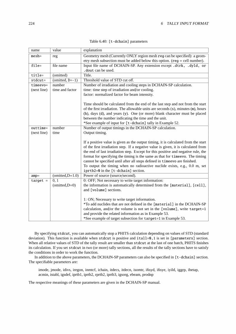
224 6 TALLY INPUT FORMAT
Table 6.40:[t-dchain] parameters
name value explanation
mesh= reg Geometry mesh (Currently ONLY region meshreg can be specified): a geom-etry mesh subsection must be added below this option. (reg = cell number).
file= file name Input file name of DCHAIN-SP. Any extension except.dtrk, .dyld, or.dout can be used.
title= (omitted) Title.stdcut= (omitted,D=-1) Threshold value of STD cut off.timeevo= number Number of irradiation and cooling steps in DCHAIN-SP calculation.(next line) time and factor time: time step of irradiation and/or cooling.
factor: normalized factor for beam intensity.
Time should be calculated from the end of the last step and not from the startof the first irradiation. The allowable units are seconds (s), minutes (m), hours(h), days (d), and years (y). One (or more) blank character must be placedbetween the number indicating the time and the unit.*See example of input for[t-dchain] tally in Example52.
outtime= number Number of output timings in the DCHAIN-SP calculation.(next line) time Output timing.
If a positive value is given as the output timing, it is calculated from the startof the first irradiation step. If a negative value is given, it is calculated fromthe end of last irradiation step. Except for this positive and negative rule, theformat for specifying the timing is the same as that fortimeevo. The timingcannot be specified until after all steps defined intimeevo are finished.To output the timing when no radioactive nuclide exists, e.g., 0.0 m, setiprtb2=0 in the[t-dchain] section.
amp= (omitted,D=1.0) Power of source (source/second).target = 0, 1 0: OFF; Not necessary to write target information:
(omitted,D=0) the information is automatically determined from the[material], [cell],and[volume] sections.
1: ON; Necessary to write target information.*To add nuclides that are not defined in the[material] in the DCHAIN-SPcalculation, and/or the volume is not set in the[volume], write target=1and provide the related information as in Example53.*See example of target subsection fortarget=1 in Example53.
By specifyingstdcut, you can automatically stop a PHITS calculation depending on values of STD (standarddeviation). This function is available whenstdcut is positive anditall=0,1 is set in[parameters] section.When all relative values of STD of the tally result are smaller thanstdcut at the last of one batch, PHITS finishesits calculation. If you setstdcut in two (or more) tally sections, all the results of the tally sections have to satisfythe conditions in order to work the function.
In addition to the above parameters, the DCHAIN-SP parameters can also be specified in[t-dchain] section.The specifiable parameters are:
imode, jmode, idivs, iregon, inmtcf, ichain, itdecs, itdecn, isomtr, ifisyd, ifisye, iyild, iggrp, ibetap,acmin, istabl, igsdef, iprtb1, iprtb2, rprtb2, iprtb3, igsorg, ebeam, prodnp
The respective meanings of these parameters are given in the DCHAIN-SP manual.

6.14 [ T-Dchain ] section 225
Example 52: Example of input for[t-dchain] tally
1: mesh = reg <-region mesh
2: reg = 100 <-cell number
3: file = testDC.spd <-file name of DCHAIN-SP input
4: title = [t-dchain] test calc.
5: amp = 1.0E12 <-source power (source/sec)
6:
7: timeevo = 4 <-number of irradiation and cooling steps
8: 3.0 h 1.0 <-irradiation for 3 hours
9: 2.0 h 0.0 <-cooling for 2 hours
10: 3.5 h 1.0 <-irradiation for 3.5 hours
11: 15.5 h 0.0 <-cooling for 15.5 hours
12:
13: outtime = 3 <-number of output timing
14: 3.0 h <-3 hours later from the 1st irradiation start time
15: -1.0 h <-1 hour later from the end of the last irradiation step
16: -3.0 h <-3 hour later from the end of the last irradiation step
Figure 6.5: Relation between steps for irradiation and cooling time and output time.
Example 53: Example for the setting of target material compositions and volumes fortarget=1
.......
: target = 1 <-target material composition ON
: non reg vol <-omissible
: 1 1 8000.0 <-serial number, cell number, volume
: tg-list = 2 <-number of the nuclides
: H-1 6.689E-02 <-Element ID, Atomic Number,
: O-16 3.345E-02 and Density of the atom (10ˆ24/cmˆ3)
: 2 2 2000.0 <-serial number, cell number, volume
: tg-list = 1 <-Number of the nuclides
: Fe-56 8.385E-02
To indicate an isotope, the symbol of the chemical element must be connected with its atomic number usingthe character ‘-.’
Important notices for using[t-dchain]:
• Only one[t-dchain] tally per PHITS input file is allowed.
• The following parameters must be defined in the[parameters] section:
– jmout=1: display the atomic number density of materials.
– file(21): set the placement of the data folder for DCHAIN-SP.
• The volume of each tally region must be defined in the[volume] section.
Files generated by[t-dchain] are listed below.
• The basic input file of DCHAIN-SP: file name is set in the[t-dchain] tally.
• Neutron energy spectra with 1968 group energy structures below 20 MeV are calculated by creating[t-track]:“n.flux.” When more than two regions are set, use the file names n.flux01, n.flux02, · · · , f.flux XX.

226 6 TALLY INPUT FORMAT
• Nuclear production yields are calculated by creating[t-yield]: “nmtc yield.”
• Information on the link to the folder containing the DCHAIN-SP data library is in “dchlink.dat.”
• Files for PHITS restart calculation:***.dtrk, ***.dyld, *** err.dyld, ***.dout
Not that when DCHAIN-SP is executed, files of names shown below are deleted.yield.out, out-gsdef, out-gamsporg, out-allreg, spd-act.out, angel-data.ang, out-phits

6.15 [ T-WWG ] section 227
6.15 [ T-WWG ] section
The[t-wwg] tally outputs parameters used for the[Weight Window] section. The tally serves as a WeightWindow Generator (WWG) to automatically obtain effective settings of[Weight Window] for a user-definedvirtual space. When using this function, a test calculation using an input file including the[t-wwg] tally must beperformed. Long calculations can then be performed using the[Weight Window] section generated from this testcalculation. The parameters are determined by the number of particles entering the cells52. In the test calculation,PHITS records the number of particles entering the cells specified in[t-wwg], and normalizes their values so asto set the maximum of the weight window to 1. If no particle arrives at a specified cell, the weight window is set tothe same value as that in the cell with the minimum fluence. This tally outputs one set of the[Weight Window]
section for each type of particle specified by part. If the energy or time mesh is defined in[t-wwg], the[WeightWindow] sections are output for each bin. You have to give volumes of each cells in[volume] section.
When you perform the restart calculation or use the sumtally function with an input file including[t-wwg],setireschk=1 in the[parameters] section.
The[t-wwg] parameters are formatted as follows.
Table 6.41:[t-wwg] parameters (1)
name value explanation
mesh = reg Geometry mesh. Onlyreg can be set.part = all (default), Maximum 6 particles in a[t-wwg].
particle namematerial = (omissible) You can specify materials for scoring.
all, all : default (same as no definition)number of materials When you set number of materials, define these material num-
bers in the next line.
(next line) 2 5 8 Material numbers.e-type = 1, 2, 3, 4, 5 Energy mesh.
You need energy mesh subsection.t-type = 1, 2, 3, 4, 5 Time mesh.
(omissible) You need time mesh subsection.unit = 1(omissible) 1: [1/cm2/source]axis = eng, reg, xy, yz, xz, x-axis value of output data.[t-track].
t, wwg It is the same as[t-track] except forwwg.To perform restart calculation, set two (or more)axis, and thenset the firstaxis to reg, eng, or t.
file = file name Define file names as same number ofaxis.resfile = (omissible,D=file) Define a file name of the past tally in the restart calculation.
Even if severalaxis parameters were defined, you should spec-ify only oneresfile.
factor = (omissible, D=1.0) Normalization factor.title = (omissible) Title.angel = (omissible) Angel parameters.rshow = 0 (default),1, 2, 3 Whenmesh=reg, axis=xy,yz,xz, region border (1), mate-
rial name (2), and region name (3) are plotted by the option.You need xyz mesh section.
Only reg can be set mesh because the parameters in[Weight Window] are defined for each region. In short,axis should be setwwg to obtain the parameters for[Weight Window]. Althougheng, reg, xy, yz, xz, andt can also be set, their results are not related with[Weight Window]. axis= xy, yz, or xz are valid onlywith rshow=1.
52 To be precise, it is determined by the fluence of a Monte Carlo particle, i.e., a particle always having weight= 1.

228 6 TALLY INPUT FORMAT
Table 6.42:[t-wwg] parameters (2)
name value explanation
ginfo = 0 (default), No geometry check in the case ofgshow> 0 orrshow> 0.1 Check geometry and draw its two-dimensional view with error infor-
mation.2 Check geometry, draw its two-dimensional view, and output a geom-
etry error file (.err).resol = 1 (default) The option multiplies region line resolution byresol times with
gshow or rshow option.width = 0.5 (default) The option defines the line thickness for gshow or rshow option.volume (omissible) The option defines volume for each region forreg mesh. You need
volume definitions below this option. Default values are given in inputecho in the case of no definition.
epsout = 0 (default), 1, 2 Whenepsout=1, results are plotted into eps files. This eps file isnamed by replacing the extension into “.eps ”.Whenepsout=2, error bars are also displayed in the eps file, exceptfor axis= xy, yz, xz, wwg.
ctmin(i) = (omissible, D=-9999) Minimum value for i-th counter.ctmax(i) = (omissible, D= 9999) Maximum value for i-th counter.trcl = (omissible) Coordinate transformation number or definition forr-z or xyz
mesh.gslat = 1(default), 0 1: show lattice boundary in gshow, 0: no.stdcut = (omissible,D=-1) Threshold value of STD cut off.
By specifyingstdcut, you can automatically stop a PHITS calculation depending on values of STD (standarddeviation). This function is available whenstdcut is positive anditall=0,1 is set in[parameters] section.When all relative values of STD of the tally result are smaller thanstdcut at the last of one batch, PHITS finishesits calculation. If you setstdcut in two (or more) tally sections, all the results of the tally sections have to satisfythe conditions in order to work the function.
An example output of this tally is as follows.
[ Weight Window ]
set: c71[0.0] c72[c71+2.13496E-08] c73[1.25478E-04]
set: c74[0.0] c75[c74+9.29569E-09] c76[2.08987E-04]
part = neutron
eng = 2
1.00000E-03 1.00000E+03
reg ww1 ww2
1 (8.94092E-05+c71)/c73 (2.08987E-04+c74)/c76
2 (1.25478E-04+c71)/c73 (1.26817E-04+c74)/c76
3 (8.53835E-05+c71)/c73 (5.78131E-05+c74)/c76
In this sample, the[Weight Window] parameters for neutrons with two energy bins are output. In principle,it is not necessary to change these parameters, butc71 or c74 should be specified when adding a constant valuefor each Weight Window.

6.16 [ T-WWBG ] section 229
6.16 [ T-WWBG ] section
The[t-wwbg] tally outputs parameters used for the[ww bias] section. The tally serves as a Weight WindowBias Generator (WWBG) to automatically obtain effective settings of[ww bias], which is used to bias[weightwindow]. The[ww bias] function is useful when the[weight window] parameters for a certain region arebiased after automatically generating the[weight window] section by[t-wwg]. Figure4.47shows a flowcharthow to perform the transport calculation using[weight window] and[ww bias]. First, generate the[weightwindow] section by[t-wwg]. If the obtained parameters of[weight window] are enough to effectively use thevariance reduction technique, the[ww bias] section is not needed. However, if they are not enough, the variancereduction technique can be used more effectively by biasing the[weight window] parameters for a certain regionwith [ww bias]. There are two methods to set the[ww bias] section; an automatic method using[t-wwbg],which is a Weight Window Bias Generator (WWBG) and will be explained below, and a manual method by auser. Only one[t-wwbg] section can be set in one input file.[t-wwbg] is effective only whenicntl=15 in[parameters]. For details of[ww bias], see Sec.4.20. When performing a transport calculation with[wwbias] and[weight window], seticntl=0 andiwwbias=1 in [parameters].
Set [weight window]・With setting [t-wwg], perform
a normal calculation (icntl=0).
([weight window] is automatically set.)
Set [ww bias]・With setting [t-wwbg], perform
a sample calculation (icntl=15).
([ww bias] is automatically set.)
or
・Set [ww bias] manually.
Transport calculation with [weight window] and [ww bias]・Set [weight window] and [ww bias] in the same input file.
・Execute PHITS with icntl=0 and iwwbias=1 in [parameters].
Figure 6.6: The flowchart of the connection calculation between[weight window] and[ww bias].
[t-wwbg] determines the bias values in stages of some cylindrical regions, which are with a central axis on avector defined by two points(x0,y0,z0) and(x1,y1,z1), shown in Fig.6.7. Figure6.7shows a cross-sectionview of three different size cylinders. To define the cylindrical regions, the parametersn-mesh, r-mesh, z-mesh,andf-mesh are also required.n-mesh is the number of the cylinders. The differences of radii and heights ofthe cylinders are given byr-mesh, z-mesh, respectively. In these parameters, the same number of values as then-mesh must be given. The bias values can be set from the inside of the cylindrical regions inf-mesh. f-meshmust be set of(n-mesh)+1. The last value off-mesh is the bias value in the outside of the cylinders. The
(x0,y0,z0) (x1,y1,z1)
rm1
rm2
rm3
zm1 zm2 zm3 fm1
fm2
fm3
fm4
Figure 6.7: Parameters to define cylindrical regions.

230 6 TALLY INPUT FORMAT
cylindrical regions can be defined regardless of the geometry to calculation of the particle transport simulation.Note that if the defined cylindrical regions overlap the outer void given in[cell], the outer void region can beextended by ther-out parameter.
The[t-wwbg] parameters are formatted as follows.
Table 6.43:[t-wwbg] parameters
name value explanation
mesh = reg Geometry mesh. Onlyreg can be set.part = all (default), Maximum 6 particles in a[t-wwg].e-type = 1, 2, 3, 4, 5 Energy mesh.
You need energy mesh subsection.t-type = 1, 2, 3, 4, 5 Time mesh.
(omissible) You need time mesh subsection.axis = xy, yz, xz, wwbg Restart calculation cannot be performed. Whenxy, yz, zx,
thershow option is needed.file = file name Define file names as same number ofaxis.angel = (omissible) Angel parameters.x-txt = (omissible) Text of x-axis.y-txt = (omissible) Text ofy-axis.z-txt = (omissible) Text ofz-axis.rshow = 0 (default),1, 2, 3 Whenmesh=reg, axis=xy,yz,xz, region border (1), mate-
rial name (2), and region name (3) are plotted by the option.You need xyz mesh section.
ginfo = 0 (default), No geometry check in the case ofgshow> 0 orrshow> 0.1 Check geometry and draw its two-dimensional view with error
information.2 Check geometry, draw its two-dimensional view, and output a
geometry error file (.err).resol = 1 (default) The option multiplies region line resolution byresol times
with gshow or rshow option.width = 0.5 (default) The option defines the line thickness forgshow or rshow op-
tion.epsout = 0 (default), 1, 2 Whenepsout=1, results are plotted into eps files. This eps file
is named by replacing the extension into “.eps ”.x0, y0, z0 = x, y, z coordinates of an initial point.x1, y1, z1 = x, y, z coordinates of a terminal point.n-mesh = n The number of cylindrical regions.r-mesh = rm1,rm2,· · · ,rmn The difference of radii of cylinders. The number ofn-mesh
must be set.z-mesh = zm1,zm2,· · · ,zmn The difference of heights of cylinders. The number ofn-mesh
must be set.f-mesh = fm1,fm2,· · · ,fmn,fm(n+1) Bias values in cylindrical regions. The number of(n-mesh)+1
must be set.r-out = (omissible, D=0) Radius to extend the outer void [cm].

6.16 [ T-WWBG ] section 231
The following is an example of[t-wwbg].
Example 54: Example of[t-wwbg].
1: [ T - WWBG ]
2: mesh = reg
3: reg = all
4: axis = wwbg
5: file = wwbg.out
6: axis = yz
7: file = wwbyz.out
8: part = neutron
9: e-type = 1
10: ne = 2
11: 0.0 1e-3 1.0
12: x0 = 0.0
13: y0 = -20
14: z0 = 50
15: x1 = 0.0
16: y1 = 20
17: z1 = 150
18: n-mesh = 3
19: r-mesh = 10 10 10
20: z-mesh = 10 10 10
21: f-mesh = 1.0 0.5 0.1 0.05
22: r-out = 1000
In this example, the initial and terminal points are (0, -20, 50) and (0, 20, 150), respectively. The three cylindricalregions are defined with the central axis on the vector defined the two points. Figure6.8shows a spatial distributionof the bias values given by the example input. The radii of the three cylinders are defined byr-mesh, the differencesof them are 10cm. The heights of the cylinders increase by 20cm, which is two times of 10cm given byz-mesh.Bias values are given as 1.0, 0.5, 0.1, and 0.05 from the inside of the cylindrical regions. The change of the biasesis shown in Fig.6.8.
File = wwbyz01.dat Date = 09:30 08-Aug-2017
plotted by ANGEL 4.35 calculated by PHITS 2.95
0 50 100 150 200
−50
0
50
z [cm]
y [c
m]
no. = 1, ix = 1
10−1
100
WW
B [W
WB
]
x = 0.0000E+00 [cm]
Figure 6.8: Spatial distribution of bias values given by the example54.

232 6 TALLY INPUT FORMAT
6.17 [ T-Volume ] section
You can automatically obtain volumes of each cell by using this tally.[t-volume] is effective only when youseticntl=14 in [parameters] section. You can set only one[t-volume] section in one input file. For detailsof the execution of this automatic calculation, see Sec.7.
The format of parameters in[t-volume] is as follows.
Table 6.44:[t-volume] parameters
name value explanation
mesh = reg Geometry mesh. Onlyreg can be set.file = file name Define an output file name.resfile = (omissible,D=file) Define a file name of the past tally in the
restart calculation.r-out = (omissible,D=0.0) Radius of outer void. (cm)title = (omissible) Title.method = (omissible, D=0) Option for Monte Carlo integration.
0: By particle track lengths.1: By source points.
s-type = 1, 2 Source type for volume calculation.1: Sphere source. The coordinates of thesphere, (x0, y0, z0), and its radius,r0, haveto be defined.2: Rectangular solid source. The coordinatesx0, x1, y0, y1, z0, andz1 have to be defined.
x0, y0, z0, Coordinates and radius.x1, y1, z1,
r0 =
stdcut = (omissible,D=-1) Threshold value of STD cut off.
You can specify the source type in the volume calculation bys-type. In s-type=1, the source generates on asphere of the center coordinates (x0,y0,z0) and the radiusr0with the inward direction. This is the same conditionasdir=-all in s-type=9 of [source] section. Ins-type=2, the source uniformly generates on surfaces of arectangular solid which are defined by 6 planes,x=x0, x1, y=y0, y1, andz=z0, z1. Its direction is inward.In either case, you have to set the source region to be large so as to cover the all specified cells.
By specifyingstdcut, you can automatically stop a PHITS calculation depending on values of STD (standarddeviation). This function is available whenstdcut is positive anditall=0,1 is set in[parameters] section.When all relative values of STD of the tally result are smaller thanstdcut at the last of one batch, PHITS finishesits calculation. If you setstdcut in two (or more) tally sections, all the results of the tally sections have to satisfythe conditions in order to work the function.
When executing PHITS using[t-volume], the information on the source used in the volume calculation isoutput in[source] of the summary filefile(6) (D=phits.out). [source] written in the input file of PHITSis not output in the summary file.
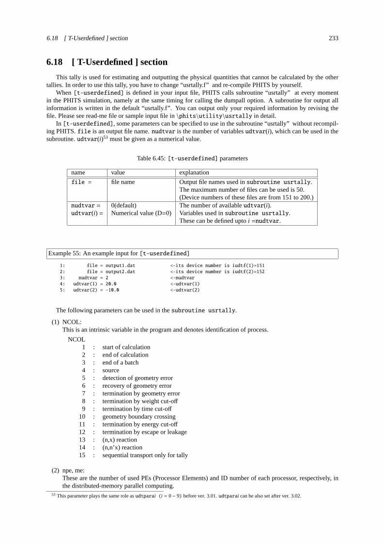
6.18 [ T-Userdefined ] section 233
6.18 [ T-Userdefined ] section
This tally is used for estimating and outputting the physical quantities that cannot be calculated by the othertallies. In order to use this tally, you have to change “usrtally.f” and re-compile PHITS by yourself.
When[t-userdefined] is defined in your input file, PHITS calls subroutine “usrtally” at every momentin the PHITS simulation, namely at the same timing for calling the dumpall option. A subroutine for output allinformation is written in the default “usrtally.f”. You can output only your required information by revising thefile. Please see read-me file or sample input file in\phits\utility\usrtally in detail.
In [t-userdefined], some parameters can be specified to use in the subroutine “usrtally” without recompil-ing PHITS.file is an output file name.nudtvar is the number of variablesudtvar(i), which can be used in thesubroutine.udtvar(i)53 must be given as a numerical value.
Table 6.45:[t-userdefined] parameters
name value explanation
file = file name Output file names used insubroutine usrtally.The maximum number of files can be used is 50.(Device numbers of these files are from 151 to 200.)
nudtvar = 0(default) The number of availableudtvar(i).udtvar(i) = Numerical value (D=0) Variables used insubroutine usrtally.
These can be defined uptoi =nudtvar.
Example 55: An example input for[t-userdefined]
1: file = output1.dat <-its device number is iudtf(1)=151
2: file = output2.dat <-its device number is iudtf(2)=152
3: nudtvar = 2 <-nudtvar
4: udtvar(1) = 20.0 <-udtvar(1)
5: udtvar(2) = -10.0 <-udtvar(2)
The following parameters can be used in thesubroutine usrtally.
(1) NCOL:This is an intrinsic variable in the program and denotes identification of process.
NCOL1 : start of calculation2 : end of calculation3 : end of a batch4 : source5 : detection of geometry error6 : recovery of geometry error7 : termination by geometry error8 : termination by weight cut-off9 : termination by time cut-off
10 : geometry boundary crossing11 : termination by energy cut-off12 : termination by escape or leakage13 : (n,x) reaction14 : (n,n’x) reaction15 : sequential transport only for tally
(2) npe, me:These are the number of used PEs (Processor Elements) and ID number of each processor, respectively, inthe distributed-memory parallel computing.
53 This parameter plays the same role asudtparai (i = 0− 9) before ver. 3.01.udtparai can be also set after ver. 3.02.

234 6 TALLY INPUT FORMAT
(3) ipomp, npomp:These are ID number of each core and the total number of used cores, respectively, in the shared memoryparallel computing.
(4) iusrtally:This is a parameter to control whethersubroutine usrtally is used or not. If[t-userdefined] isdefined in an input file, this parameter is set to be 1.
(5) iudtf(50):These are device numbers of output files defined withfile=. For example, if there is the earliest file definedin [t-userdefined], its device number isiudtf(1)=151.
(6) nudtvar:The number of availableudtvar(i). This is given asnudtvar in the input file.
(7) udtvar(i):These are numerical values defined asudtvar(i) in the input file.udtvar(i) upto i=nudtvar can be used.If udtvar(i) is not defined in the input file, it is set to 0.
(8) NOCAS, NOBCH, RCASC, RSOUIN:
NOCAS : current history number in this batchNOBCH : current batch numberRCASC : real number of NOCAS+maxcas*(NOBCH-1)RSOUIN : sum of the weight of source particle
(9) NO, IDMN, ITYP, KTYP, JTYP, MTYP, RTYP, OLDWT:
NO : cascade id in this historyIDMN : material idITYP : particle typeKTYP : particle kf-codeJTYP : charge number of the particleMTYP : baryon number of the particleRTYP : rest mass of the particle (MeV)OLDWT : wight of the particle at (x,y,z)
(10) QS:This isdE/dx for electrons at (x,y,z).
(11) IBLZ1, IBLZ2, ILEV1, ILEV2:
IBLZ1 : cell id at (x,y,z)IBLZ2 : cell id after crossingILEV1 : level structure id of the cell at (x,y,z)ILEV2 : level structure id of the cell after crossing
(a) ILAT1:This is a variable of level structure of cell.
(b) ILAT2:This is a variable of level structure of cell.
(12) COSTH, UANG(1), UANG(2), UANG(3), NSURF:
COSTH : cosine of an angle of incidence in a surface crossingUANG(1,2,3) : x,y,z component of a normal vector of its surface, respectivelyNSURF : internal number of the surface
(This is different from the surface number defined in the[surface] section.)

6.18 [ T-Userdefined ] section 235
(13) NAME, NCNT(1), NCNT(2), NCNT(3):
NAME : collision number of the particleNCNT(1,2,3) : values of counter 1, 2, and 3
(14) WT, U, V, W:
WT : wight of the particle at (xc,yc,zc)U, V, W : unit vector of momentum of the particle
(15) E, T, X, Y, Z:
E : energy of the particle at (x,y,z) (MeV)T : time of the particle at (x,y,z) (nsec)X, Y, Z : position coordinate of the preceding event point (cm)
(16) EC, TC, XC, YC, ZC:
EC : energy of the particle at (xc,yc,zc) (MeV)TC : time of the particle at (xc,yc,zc) (nsec)XC, YC, ZC : position coordinate of the particle (cm)
(17) SPX, SPY, SPZ:
SPX, SPY, SPZ : unit vector of spin direction of the particle
(18) NZST:This is charge state of the particle.
(19) NCLSTS:This variable means the number of produced particle and nucleus.
(a) MATHZ, MATHN, JCOLL, KCOLL:
MATHZ : Z number of the mother nucleusMATHN : N number of the mother nucleusJCOLL : reaction type id1KCOLL : reaction type id2
JCOLL and KCOLL indicate the following meaning.
JCOLL0 : nothing happen1 : Hydrogen collisions2 : Particle Decays3 : Elastic collisions4 : High Energy Nuclear collisions5 : Heavy Ion reactions6 : Neutron reactions by data7 : Photon reactions by data8 : Electron reactions by data9 : Proton reactions by data
10 : Neutron event mode11 : delta ray production13 : Photon reactions by EGS514 : Electron reactions by EGS5

236 6 TALLY INPUT FORMAT
KCOLL0 : normal1 : high energy fission2 : high energy absorption3 : low energy n elastic4 : low energy n non-elastic5 : low energy n fission6 : low energy n absorption
(b) ICLUSTS, JCLUSTS, QCLUSTS, JCOUNT:These variables have a array and denote the information on the produced particle and nucleus.
ICLUSTS kind of particle0 : nucleus1 : proton2 : neutron3 : pion4 : photon5 : kaon6 : muon7 : others
JCLUSTS(i)i = 0 : angular momentum= 1 : proton number= 2 : neutron number= 3 : ityp= 4 : status of the particle 0: real,<0 : dead= 5 : charge number= 6 : baryon number= 7 : kf code
QCLUSTS(i)i = 0 : impact parameter= 1 : px (GeV/c)= 2 : py (GeV/c)= 3 : pz (GeV/c)= 4 : etot =
√p2 +m2 (GeV)
= 5 : rest mass (GeV)= 6 : excitation energy (MeV)= 7 : kinetic energy (MeV)= 8 : weight= 9 : time (nsec)= 10 : x coordinate (cm)= 11 : y coordinate (cm)= 12 : z coordinate (cm)

6.19 [ T-Gshow ] section 237
6.19 [ T-Gshow ] section
[ T - G s h o w ] gives graphical geometry output for region boundary by xyz mesh. You can obtain theseresults without transport calculations withicntl =7 option in the [parameters] section.
Table 6.46:[t-gshow] parameter
name value explanation
mesh = xyz geometry mesh, only xyz meshyou need geometry mesh subsection below this option
axis = xy, yz, xz 2 dimensionalfile = file name Define file names as same number of axisoutput = 1 region boundary
2 region boundary+ material color3 region boundary+ material name4 region boundary+ material color+ material name5 region boundary+ region name6 region boundary+ material color+ region name7 region boundary+ LAT number8 region boundary+ material color+ LAT number
resol = 1 (default) The resolution in displaying region lines is multiplied by this value.width = 0.5 (default) The thickness of displayed region lines.title = (omissible) titleangel = (omissible) angel parameterssangel = (omissible) sangel parametersx-txt = (omissible) x axis titley-txt = (omissible) y axis titleepsout = 0 (default), 1 If epsout is set to 1, results are plotted
into eps files. This eps file is namedby replacing the extension into “.eps”.
bmpout = 0(default), 1 Generate Bitmap figure of 2-dimensional tally output.This file is named by replacing the extension into “.bmp ”.Whenmesh=xyz, axis=(xy, yz, or xz), this is available.
vtkout = 0(default), 1 Output the tally results in xyz-mesh in the input format of ParaView.This file is named by replacing the extension into “.vtk ”.Whenmesh=xyz, axis=(xy, yz, or xz), this is available.
vtkfmt = 0(default), 1 Format of output file for ParaView.0: ascii, 1: binary.
trcl = (omissible) coordinate transformation number or definitionfor r-z or xyz mesh
gslat = 1(default), 0 1: show lattice boundary in gshow, 0: noginfo = 2 (default), Region error check
0 No geometry check1 Check geometry and draw its two-dimensional view
with error information2 Check geometry, draw its two-dimensional view,
and outputting a geometry error file (.err)

238 6 TALLY INPUT FORMAT
output=7,8 can be used only when cells in bottom level are the lattice themselves, and they give latticenumber in the format as (4,1,2). For example, Fig.4.40in Sec.4.6.4is generated by the input shown below.
Example 56:[t-gshow] example
1: [ T - gshow ]
2: mesh = xyz
3: x-type = 2
4: nx = 100
5: xmin = -10.
6: xmax = 10
7: y-type = 1
8: ny = 1
9: -5.0 5.0
10: z-type = 2
11: nz = 100
12: zmin = -10.
13: zmax = 10.
14: axis = xz
15: output = 8
16: file = cell-example6.dat
17: epsout = 1

6.20 [ T-Rshow ] section 239
6.20 [ T-Rshow ] section
[ T - R s h o w ] gives graphical geometry output for region boundary with color plot region in proportionto physical quantity of the region. Usually, the results obtained by other PHITS calculation using the reg meshare used as the input data for this value of physical quantity. You must run PHITS withicntl =9 option in the[parameters] section, in order to execute this tally.
You can give color variation by the linear scale or the log scale by the ANGEL parameter, zlog or zlin. Defaultis zlin.
Table 6.47:[t-rshow] parameter
name value explanation
mesh = xyz geometry mesh, only xyz meshyou need geometry mesh subsection below this option
axis = xy, yz, xz 2 dimensionalfile = file name Define file names as same number of axisoutput = 1 region boundary
2 region boundary+ material name3 region boundary+ region name4 region boundary+ LAT number
resol = 1 (default) The resolution in displaying region lines is multiplied by this value.width = 0.5 (default) The thickness of displayed region lines.title = (omissible) titleangel = (omissible) angel parameterssangel = (omissible) sangel parametersx-txt = (omissible) x axis titley-txt = (omissible) y axis titlez-txt = (omissible) z axis titlereg = region definitionvaluereg val value definition with same format as volume definition
see section5.1.2iechrl = 72 (default) Number of maximum column for volume input echoepsout = 0 (default), 1 If epsout is set to 1, results are plotted
into eps files. This eps file is namedby replacing the extension into “.eps”.
bmpout = 0(default), 1 Generate Bitmap figure of 2-dimensional tally output.This file is named by replacing the extension into “.bmp ”.Whenmesh=xyz, axis=(xy, yz, or xz), this is available.
trcl = (omissible) coordinate transformation number or definitionfor r-z or xyz mesh
gslat = 1(default), 0 1: show lattice boundary in gshow, 0: noginfo = 2 (default), Region error check
0 No geometry check1 Check geometry and draw its two-dimensional view
with error information2 Check geometry, draw its two-dimensional view,
and outputting a geometry error file (.err)

240 6 TALLY INPUT FORMAT
For example, you can obtain Fig.6.9by the[t-rshow] tally shown below from the example (6) in Sec.4.6.4.
Example 57:[t-rshow] example
1: [ T - rshow ]
2: mesh = xyz
3: x-type = 2
4: nx = 100
5: xmin = -10.
6: xmax = 10.
7: y-type = 1
8: ny = 1
9: -5.0 5.0
10: z-type = 2
11: nz = 100
12: zmin = -10.
13: zmax = 10.
14: axis = xz
15: output = 1
16: file = cell-example6-rshow.dat
17: epsout = 1
18: reg = (201<101[-1 1 0]<1) (201<101[0 1 0]<1) (201<101[1 1 0]<1)
19: (201<101[-1 0 0]<1) (201<101[0 0 0]<1) (201<101[1 0 0]<1)
20: (201<101[-1 -1 0]<1) (201<101[0 -1 0]<1) (201<101[1 -1 0]<1)
21: value
22: non reg val # reg definition
23: 1 1000001 1.0000E+00 # ( 201 < 101[ -1 1 0 ] < 1 )
24: 2 1000002 2.0000E+00 # ( 201 < 101[ 0 1 0 ] < 1 )
25: 3 1000003 3.0000E+00 # ( 201 < 101[ 1 1 0 ] < 1 )
26: 4 1000004 4.0000E+00 # ( 201 < 101[ -1 0 0 ] < 1 )
27: 5 1000005 5.0000E+00 # ( 201 < 101[ 0 0 0 ] < 1 )
28: 6 1000006 6.0000E+00 # ( 201 < 101[ 1 0 0 ] < 1 )
29: 7 1000007 7.0000E+00 # ( 201 < 101[ -1 -1 0 ] < 1 )
30: 8 1000008 8.0000E+00 # ( 201 < 101[ 0 -1 0 ] < 1 )
31: 9 1000009 9.0000E+00 # ( 201 < 101[ 1 -1 0 ] < 1 )
−10 −5 0 5 10−10
−5
0
5
10
z [cm]
x [c
m]
100
Val
ues
Figure 6.9:Example of[t-rshow].

6.21 [ T-3Dshow ] section 241
6.21 [ T-3Dshow ] section
[ T - 3 D s h o w ] gives a graphical geometry output by 3 dimensional view. You can execute this tally withicntl =11 option in the [parameters] section without transport calculations.
Table 6.48:[t-3dshow] parameter (1)
name value explanation
output = 0 draft1 only region boundary2 without region boundary3 (default) region boundary+ color
material = (omissible) You can specify materials for display.all, all : default (same as no definition)number of materials When you set number of materials,
define these material numbers in the next line.You can set number of materials by negative.In the case, specified materials are not includedfor display.
(next line) 2 5 8 material numbersx0 = (D=0.0) Coordinates of original point for view pointy0 = (D=0.0) and light source. Center of screen is definedz0 = (D=0.0) by this point and view pointe-the = (D=80) view point angleθ(degree) with z axise-phi = (D=140) azimuthal angle for view pointϕ(degree) with x axise-dst = (D=w-dst*10) distance between view point and the origin (cm)l-the = (D=e-the) light source angleθ(degree) with z axisl-phi = (D=e-phi) azimuthal angle for light sourceϕ(degree) with x axisl-dst = (D=e-dst) distance between light source and the origin (cm)w-wdt = (D=100) width of screen frame (cm)w-hgt = (D=100) height of screen frame(cm)w-dst = (D=200) screen frame distance from the origin (cm)
A straight line drawn between the center of screen frameand the origin crosses screen surface vertically,and passes through the view point.
w-mnw = (D=100) number of mesh for horizontal directionw-mnh = (D=100) number of mesh for vertical directionw-ang = (D=0.0) angle of frame (degree)heaven = (D=y) topside direction; set x, -x, y, -y, z, or -zmirror = (D=0) =-1; mirror transformation in horizontal direction

242 6 TALLY INPUT FORMAT
Origin (x0,y0,z0)
(e-the,e-phi,e-dst)
w-hgt
(w-mnh)
w-dst
w-wdt
(w-mnw)
e-dst
Picture FlameEye Point
Light source
(l-the,l-phi,l-dst)
w-mnw w-mnh #Pixel
100 100 (default)
Polar
Coordinates
Polar
coordinates
XYZ-coordinates
Figure 6.10: 3dshow tally: origin (x0,y0,z0), eye point (e-the,e-phi,e-dst), light source(l-the,l-phi,l-dst), and picture flame (w-wdt,w-hgt,w-dst).

6.21 [ T-3Dshow ] section 243
Table 6.49:[t-3dshow] parameter (2)
name value explanation
line = 0 (default),1 When output= 1, 30: material boundary+ surface boundary1: material boundary+ surface boundary+ region boundary
r-out = (D=50000) radius of outer void including view point,and light source(cm)
shadow = (D=0) shadow level (0:no shadow, 2 is recommended)bright = (D=0.8) brightness limit (1:max, 0:no brightness)dark = (D=0.2) darkness limit (1:no darkness, 0:max)box = (D=0) number of penetration box, maximum 5box 10 numbers box definition (see below)matinbox = (omissible) materials in the box for display
all, all : default (same with no definition)number of materials When you set number of materials,
define these material numbers in the next line.You cannot set number of materials by negative.
(next line) 2 5 8 material numbersreginbox = (omissible) regions in the box for display
all, all : default (same with no definition)region numbers If the matinbox is defined for this region,
this region is not displayed.resol = 1 (default) The resolution in displaying region lines is multiplied by this value.width = 0.5 (default) The thickness of displayed region lines.file = file name Define file names as same number of axistitle = (omissible) titleangel = (omissible) angel parameterssangel = (omissible) sangel parametersx-txt = (omissible) x axis titley-txt = (omissible) y axis titlez-txt = (omissible) z axis titleepsout = 0 (default), 1 If epsout is set to 1, results are plotted
into eps files. This eps file is namedby replacing the extension into “.eps”.
axishow = (D=1) 0, 1, 2 0: No.1: Small axis is shown in the lower-left of a figure.2: Large axis is shown in the center of a figure.
Definition rules forreg=, andreginbox = are the same as that for the region mesh in section5.1.1.For saving calculating time, an outer region defined by the radiusr-out is introduced additionally. You have
to use a largerr-out value when you use large geometry, or you want to put the light source and view point faraway. This new definition of the outer region can be seen in input echo. Therefore, you cannot use an input echoby icntl=11 as an input for next calculation.
Shadow is not created if the view point and light source are set same position.

244 6 TALLY INPUT FORMAT
6.21.1 box definition
Maximum 5 penetration boxes can be defined. Defined boxes become transparent. To define the box, you firstset three points asb0(x0,y0,z0), b1(x1,y1,z1), andb2(x2,y2,z2). We define the 4-th pointb3 from b0 by L cm on thevertical direction of the plane defined by these three points, i.e. (b2 - b0 ) direction. In thisbox definition, you canuse the coordinate transformation astrcl = transform number ortrcl = (........) before the definition ofthe points.
This function may fail when a void region is included in the penetration box. In this case, please fill the voidregion with a material of very low density, e.g. air.
The box definition is shown below. Each relations are also shown in Fig.6.11.
box = 2
box x0 y0 z0
x1 y1 z1
x2 y2 z2 L
box trcl = 2
x0 y0 z0
x1 y1 z1
x2 y2 z2 L
box *trcl = (0 0 0 0 90 90 90 60 150 90 30 60 -1)
0.0 0.0 0.0
-5.0 0.0 0.0
0.0 0.0 5.0 5.0
L
( x0 , y0 , z0 )
( x1 , y1 , z1 )
( x2 , y2 , z2 )
( x3 , y3 , z3 )
Figure 6.11:Example of box definition.

6.21 [ T-3Dshow ] section 245
6.21.2 3dshow example
Example 58:[t-3dshow] example (1)
1: [cell]
2: 1 0 -1 fill=1
3: 2 0 -41 42 -43 44 -45 46 u=1 fill=5
4: 22 0 -41 42 -43 44 -45 46 u=1 trcl=(0 0 20) fill=6
5: 23 like 22 but trcl=(0 0 40) fill = 7
6: 5 0 -21 22 -23 24 -25 26 u=5 lat=1 fill=3
7: 6 0 -21 22 -23 24 -25 26 u=6 lat=1 fill= -1:1 0:0 0:0 2 2(0 0 5) 2
8: 7 0 -21 22 -23 24 -25 26 u=7 fill= -1:1 0:0 0:0 2 3 2 lat=1
9: 3 1 3.97300E-02 3 u=2
10: 4 6 4.18280E-02 -3 u=2
11: 13 5 8.47130E-04 -3 u=3
12: 14 3 1.23620E-01 3 u=3
13: 8 -1 +1
14: [surface]
15: 1 rpp -15 15 -5 5 -5 55
16: 21 px 5
17: 22 px -5
18: 23 py 5
19: 24 py -5
20: 25 pz 15
21: 26 pz -5
22: 41 px 15
23: 42 px -15
24: 43 py 5
25: 44 py -5
26: 45 pz 15
27: 46 pz -5
28: 5 rpp -20 20 -5 5 -5 35
29: 6 rpp -20 20 -5 5 -5 15
30: 7 rpp -20 20 -5 5 35 55
31: 3 c/y 0 10 4
In above geometry, the whole body is rectangular solid, and it has rectangular solid lattices including cylindersinside. You can make graphical plot for the geometry by the 3dshow as,
Example 59:[t-3dshow] example (2)
1: [t-3dshow]
2: output = 3
3: heaven = x
4: resol = 2
5: width = 0.1
6: x0 = 0
7: y0 = 0
8: z0 = 25
9: e-the = 70
10: e-phi = 50
11: e-dst = 1000
12: l-the = 50
13: l-phi = 25
14: l-dst = 2000
15: w-wdt = 60
16: w-hgt = 40
17: w-dst = 150
18: file = dshow.dat

246 6 TALLY INPUT FORMAT
The output result is ,
You can add region boundary by optionline=1 as,
You can see how lattices are set up. Next, let material number 5 be transparent, and add shadows by
material = -1
5
shadow = 2

6.21 [ T-3Dshow ] section 247
Let’s define a box.
box = 1
box 0 10 30
100 10 30
0 10 100 100
The defined box part becomes transparent, and you can see inside of the body.
In the last example, add
reg = ( 3 < 6[0 0 0] )
matinbox = 1
6
Regions defined byreg = (3 < 6[0 0 0] ) become transparent, and material number 6 becomes visible.
You can display any complex structures as you like combining with these options.

248 7 AUTOMATIC CALCULATION OF REGION VOLUME
7 Automatic calculation of region volume
When you setmesh=reg in tally sections, you have to give volumes of each cell to estimate results in the unitof (/volume). PHITS has a function of automatic calculation to obtain the volumes. The instruction how to use thisfunction is shown below.
In this function, PHITS calculates the volumes by performing a Monte Carlo integration with setting the ma-terial of each cell to be void and a special source region. When you use this function, set[t-volume] sectionandicntl=14 in [parameters] section. An example of[t-volume] is as follows. For details of parameters of[t-volume], see Sec.6.17.
Example 60: Example of[t-volume]
1: [ T - V o l u m e ]
2: mesh = reg # mesh type is region-wise
3: reg = 101 102 103 104 105
4: file = volume.out # file name of output for [volume]
5: s-type = 1 # 1: Sphere source, 2: Rectangular source
6: x0 = 0.0 # (D=0.0) x of sphere center
7: y0 = 0.0 # (D=0.0) y of sphere center
8: z0 = 0.0 # (D=0.0) z of sphere center
9: r0 = 50.0 # radius of sphere
[t-volume] section should have the setting ofmesh=reg. The cell numbers should be specified afterreg=. Bysettings-type and the related parameters such asx0, you can define the special source region for the volumecalculation. Note that the source region should be set to cover all cells specified inreg=, otherwise the calculatedvolumes would be wrong. On the contrary, if you set an extremely large source region, the statistical uncertaintiesof the calculated results would be large. The obtained volumes are outputted in a file named byfile=. The formatof the output file is as follows.
[ T - V o l u m e ] off
mesh = reg # mesh type is region-wise
.... .... .... ....
.... .... .... ....
[ V o l u m e ]
non reg vol non
1 101 5.0370E+02 0.2909
2 102 2.4727E+03 0.1634
.... .... .... ....
.... .... .... ....
# Information for Restart Calculation
.... .... .... ....
.... .... .... ....
Because the volumes are outputted in the format of[volume] section, the results can be used in the main calcu-lation withicntl=0 by infl command. Here, values of the last column in[volume] are statistical uncertainties(relative values). If the uncertainties are large, you can perform the restart calculation by addingistdev=-1 or
-2 in [parameters] section, because the output file of[t-volume] has information for the restart mode.
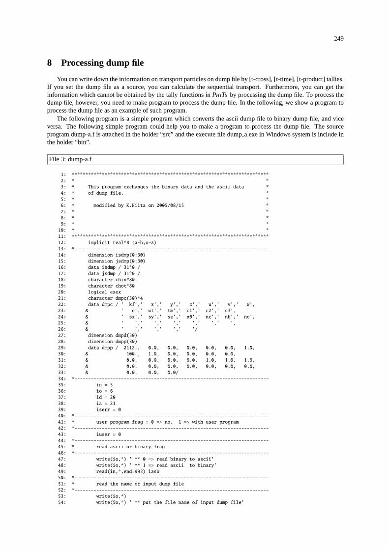
249
8 Processing dump file
You can write down the information on transport particles on dump file by [t-cross], [t-time], [t-product] tallies.If you set the dump file as a source, you can calculate the sequential transport. Furthermore, you can get theinformation which cannot be obtained by the tally functions inPHITS by processing the dump file. To process thedump file, however, you need to make program to process the dump file. In the following, we show a program toprocess the dump file as an example of such program.
The following program is a simple program which converts the ascii dump file to binary dump file, and viceversa. The following simple program could help you to make a program to process the dump file. The sourceprogram dump-a.f is attached in the holder “src” and the execute file dumpa.exe in Windows system is include inthe holder “bin”.
File 3: dump-a.f
1: ************************************************************************
2: * *
3: * This program exchanges the binary data and the ascii data *
4: * of dump file. *
5: * *
6: * modified by K.Niita on 2005/08/15 *
7: * *
8: * *
9: * *
10: * *
11: ************************************************************************
12: implicit real*8 (a-h,o-z)
13: *-----------------------------------------------------------------------
14: dimension isdmp(0:30)
15: dimension jsdmp(0:30)
16: data isdmp / 31*0 /
17: data jsdmp / 31*0 /
18: character chin*80
19: character chot*80
20: logical exex
21: character dmpc(30)*4
22: data dmpc / ’ kf’,’ x’,’ y’,’ z’,’ u’,’ v’,’ w’,
23: & ’ e’,’ wt’,’ tm’,’ c1’,’ c2’,’ c3’,
24: & ’ sx’,’ sy’,’ sz’,’ n0’,’ nc’,’ nb’,’ no’,
25: & ’ ’,’ ’,’ ’,’ ’,’ ’,’ ’,
26: & ’ ’,’ ’,’ ’,’ ’/
27: dimension dmpd(30)
28: dimension dmpp(30)
29: data dmpp / 2112., 0.0, 0.0, 0.0, 0.0, 0.0, 1.0,
30: & 100., 1.0, 0.0, 0.0, 0.0, 0.0,
31: & 0.0, 0.0, 0.0, 0.0, 1.0, 1.0, 1.0,
32: & 0.0, 0.0, 0.0, 0.0, 0.0, 0.0, 0.0,
33: & 0.0, 0.0, 0.0/
34: *-----------------------------------------------------------------------
35: in = 5
36: io = 6
37: id = 20
38: ia = 21
39: iserr = 0
40: *-----------------------------------------------------------------------
41: * user program frag : 0 => no, 1 => with user program
42: *-----------------------------------------------------------------------
43: iuser = 0
44: *-----------------------------------------------------------------------
45: * read ascii or binary frag
46: *-----------------------------------------------------------------------
47: write(io,*) ’ ** 0 => read binary to ascii’
48: write(io,*) ’ ** 1 => read ascii to binary’
49: read(in,*,end=993) iasb
50: *-----------------------------------------------------------------------
51: * read the name of input dump file
52: *-----------------------------------------------------------------------
53: write(io,*)
54: write(io,*) ’ ** put the file name of input dump file’
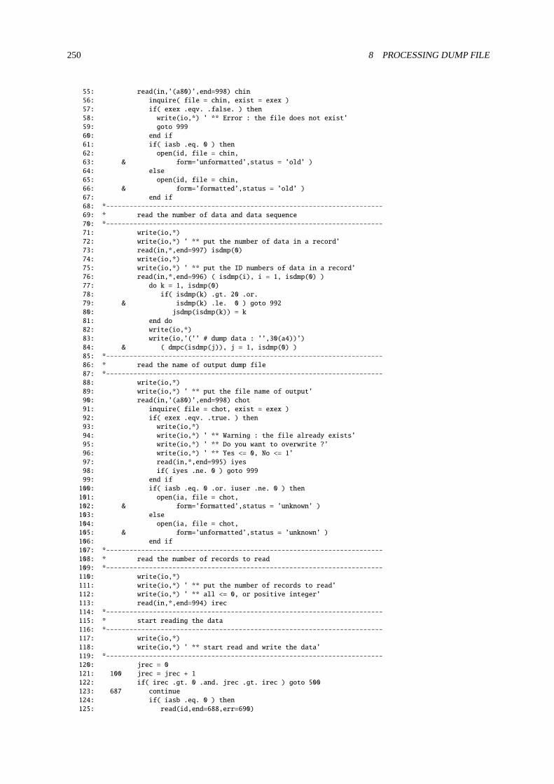
250 8 PROCESSING DUMP FILE
55: read(in,’(a80)’,end=998) chin
56: inquire( file = chin, exist = exex )
57: if( exex .eqv. .false. ) then
58: write(io,*) ’ ** Error : the file does not exist’
59: goto 999
60: end if
61: if( iasb .eq. 0 ) then
62: open(id, file = chin,
63: & form=’unformatted’,status = ’old’ )
64: else
65: open(id, file = chin,
66: & form=’formatted’,status = ’old’ )
67: end if
68: *-----------------------------------------------------------------------
69: * read the number of data and data sequence
70: *-----------------------------------------------------------------------
71: write(io,*)
72: write(io,*) ’ ** put the number of data in a record’
73: read(in,*,end=997) isdmp(0)
74: write(io,*)
75: write(io,*) ’ ** put the ID numbers of data in a record’
76: read(in,*,end=996) ( isdmp(i), i = 1, isdmp(0) )
77: do k = 1, isdmp(0)
78: if( isdmp(k) .gt. 20 .or.
79: & isdmp(k) .le. 0 ) goto 992
80: jsdmp(isdmp(k)) = k
81: end do
82: write(io,*)
83: write(io,’(’’ # dump data : ’’,30(a4))’)
84: & ( dmpc(isdmp(j)), j = 1, isdmp(0) )
85: *-----------------------------------------------------------------------
86: * read the name of output dump file
87: *-----------------------------------------------------------------------
88: write(io,*)
89: write(io,*) ’ ** put the file name of output’
90: read(in,’(a80)’,end=998) chot
91: inquire( file = chot, exist = exex )
92: if( exex .eqv. .true. ) then
93: write(io,*)
94: write(io,*) ’ ** Warning : the file already exists’
95: write(io,*) ’ ** Do you want to overwrite ?’
96: write(io,*) ’ ** Yes <= 0, No <= 1’
97: read(in,*,end=995) iyes
98: if( iyes .ne. 0 ) goto 999
99: end if
100: if( iasb .eq. 0 .or. iuser .ne. 0 ) then
101: open(ia, file = chot,
102: & form=’formatted’,status = ’unknown’ )
103: else
104: open(ia, file = chot,
105: & form=’unformatted’,status = ’unknown’ )
106: end if
107: *-----------------------------------------------------------------------
108: * read the number of records to read
109: *-----------------------------------------------------------------------
110: write(io,*)
111: write(io,*) ’ ** put the number of records to read’
112: write(io,*) ’ ** all <= 0, or positive integer’
113: read(in,*,end=994) irec
114: *-----------------------------------------------------------------------
115: * start reading the data
116: *-----------------------------------------------------------------------
117: write(io,*)
118: write(io,*) ’ ** start read and write the data’
119: *-----------------------------------------------------------------------
120: jrec = 0
121: 100 jrec = jrec + 1
122: if( irec .gt. 0 .and. jrec .gt. irec ) goto 500
123: 687 continue
124: if( iasb .eq. 0 ) then
125: read(id,end=688,err=690)
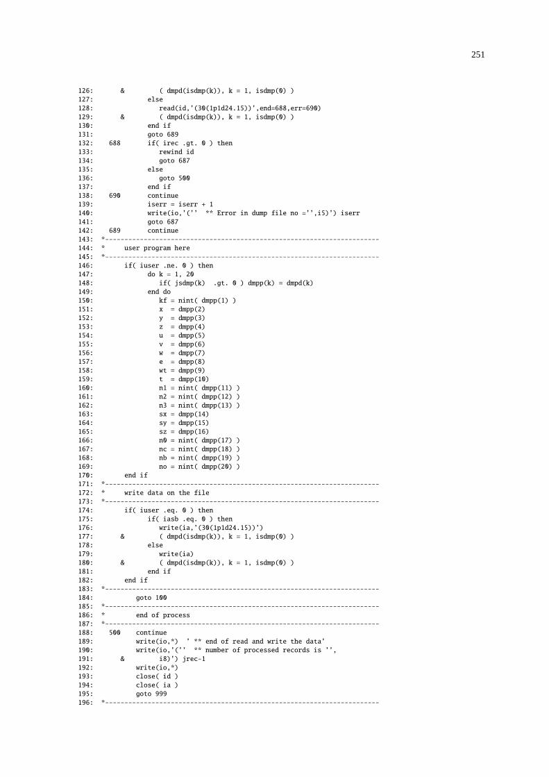
251
126: & ( dmpd(isdmp(k)), k = 1, isdmp(0) )
127: else
128: read(id,’(30(1p1d24.15))’,end=688,err=690)
129: & ( dmpd(isdmp(k)), k = 1, isdmp(0) )
130: end if
131: goto 689
132: 688 if( irec .gt. 0 ) then
133: rewind id
134: goto 687
135: else
136: goto 500
137: end if
138: 690 continue
139: iserr = iserr + 1
140: write(io,’(’’ ** Error in dump file no =’’,i5)’) iserr
141: goto 687
142: 689 continue
143: *-----------------------------------------------------------------------
144: * user program here
145: *-----------------------------------------------------------------------
146: if( iuser .ne. 0 ) then
147: do k = 1, 20
148: if( jsdmp(k) .gt. 0 ) dmpp(k) = dmpd(k)
149: end do
150: kf = nint( dmpp(1) )
151: x = dmpp(2)
152: y = dmpp(3)
153: z = dmpp(4)
154: u = dmpp(5)
155: v = dmpp(6)
156: w = dmpp(7)
157: e = dmpp(8)
158: wt = dmpp(9)
159: t = dmpp(10)
160: n1 = nint( dmpp(11) )
161: n2 = nint( dmpp(12) )
162: n3 = nint( dmpp(13) )
163: sx = dmpp(14)
164: sy = dmpp(15)
165: sz = dmpp(16)
166: n0 = nint( dmpp(17) )
167: nc = nint( dmpp(18) )
168: nb = nint( dmpp(19) )
169: no = nint( dmpp(20) )
170: end if
171: *-----------------------------------------------------------------------
172: * write data on the file
173: *-----------------------------------------------------------------------
174: if( iuser .eq. 0 ) then
175: if( iasb .eq. 0 ) then
176: write(ia,’(30(1p1d24.15))’)
177: & ( dmpd(isdmp(k)), k = 1, isdmp(0) )
178: else
179: write(ia)
180: & ( dmpd(isdmp(k)), k = 1, isdmp(0) )
181: end if
182: end if
183: *-----------------------------------------------------------------------
184: goto 100
185: *-----------------------------------------------------------------------
186: * end of process
187: *-----------------------------------------------------------------------
188: 500 continue
189: write(io,*) ’ ** end of read and write the data’
190: write(io,’(’’ ** number of processed records is ’’,
191: & i8)’) jrec-1
192: write(io,*)
193: close( id )
194: close( ia )
195: goto 999
196: *-----------------------------------------------------------------------
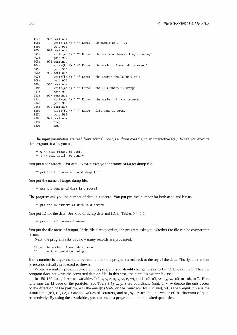
252 8 PROCESSING DUMP FILE
197: 992 continue
198: write(io,*) ’ ** Error : ID should be 1 - 20’
199: goto 999
200: 993 continue
201: write(io,*) ’ ** Error : the ascii or binary frag is wrong’
202: goto 999
203: 994 continue
204: write(io,*) ’ ** Error : the number of records is wrong’
205: goto 999
206: 995 continue
207: write(io,*) ’ ** Error : the answer should be 0 or 1’
208: goto 999
209: 996 continue
210: write(io,*) ’ ** Error : the ID numbers is wrong’
211: goto 999
212: 997 continue
213: write(io,*) ’ ** Error : the number of data is wrong’
214: goto 999
215: 998 continue
216: write(io,*) ’ ** Error : file name is wrong’
217: goto 999
218: 999 continue
219: stop
220: end
The input parameters are read from normal input, i.e. from console, in an interactive way. When you executethe program, it asks you as,
** 0 => read binary to ascii
** 1 => read ascii to binary
You put 0 for binary, 1 for ascii. Next it asks you the name of target dump file.
** put the file name of input dump file
You put the name of target dump file.
** put the number of data in a record
The program ask you the number of data in a record. You put positive number for both ascii and binary.
** put the ID numbers of data in a record
You put ID for the data. See kind of dump data and ID, in Tables5.4, 5.5.
** put the file name of output
You put the file name of output. If the file already exists, the program asks you whether the file can be overwrittenor not.
Next, the program asks you how many records are processed.
** put the number of records to read
** all <= 0, or positive integer
If this number is larger than total record number, the program turns back to the top of the data. Finally, the numberof records actually processed is shown.
When you make a program based on this program, you should changeiuser to 1 at 35 line in File3. Then theprogram does not write the converted data on file. In this case, the output is written by ascii.
In 150-169 lines, there are variables “kf, x, y, z, u, v, w, e, wt, t, n1, n2, n3, sx, sy, sz, n0, nc, nb, no”. Herekf means the kf-code of the particles (see Table3.4), x, y, z are coordinate (cm), u, v, w denote the unit vectorof the direction of the particle, e is the energy (MeV, or MeV/nucleon for nucleus), wt is the weight, time is theinitial time (ns), c1, c2, c3 are the values of counters, and sx, sy, sz are the unit vector of the direction of spin,respectively. By using these variables, you can make a program to obtain desired quantities.

253
9 Output cutoff data format
The information for neutron, photon, electron, positron, and proton below the cut off energy can be written inthe output file (file(12), file(13), and file(10)), in order to continue these transport calculation by other Monte Carlocodes such as MCNP and EGS4. The data are written in binary. The format is shown below.
rd, rn, ( data(i), i = 1, nint(abs(rd)) )
rd, rn, ( data(i), i = 1, nint(abs(rd)) )
................
................
First, in the case ofincut = 1, and no importance option (rd<0)
rd, rn, x, y, z, ( e(i), u(i), v(i), w(i), i = 1, n )
rd, rn, x, y, z, ( e(i), u(i), v(i), w(i), i = 1, n )
................
................
Next,incut =1 with importance option (rd>0),
rd, rn, x, y, z, ( e(i), u(i), v(i), w(i), wt(i), i = 1, n )
rd, rn, x, y, z, ( e(i), u(i), v(i), w(i), wt(i), i = 1, n )
................
................
incut = 2 and no importance option (rd<0),
rd, rn, x, y, z, ( e(i), u(i), v(i), w(i), t(i), i = 1, n )
rd, rn, x, y, z, ( e(i), u(i), v(i), w(i), t(i), i = 1, n )
................
................
incut = 2 with importance option (rd>0),
rd, rn, x, y, z, ( e(i), u(i), v(i), w(i), wt(i), t(i), i = 1, n )
rd, rn, x, y, z, ( e(i), u(i), v(i), w(i), wt(i), t(i), i = 1, n )
................
................
wheren = nint(rn), x, y, z is a coordinate (cm),e(i) is an energy (MeV),u(i), v(i), w(i) is an unitvector of momentum,wt(i) is an weight, andt(i) is time (ns). In the caseigcut =3, the particle identifierp(i)is written instead oft(i) in the case ofincut =2.p(i) = 3.0 is photon,p(i) = 4.0 is electron, andp(i) = 5.0 is positron.

254 10 REGION ERROR CHECK
10 Region error check
When you make a complex geometry, it is difficult to set up the geometry without any mistakes such as doubledefined and undefined regions. Thus, a function for automatically detecting double defined or undefined regionswas implemented after version 2.67. This geometry check function works when you specify a tally for generatingthe two-dimensional view of your geometry; namely[t-gshow], [t-rshow], and other tallies with settingaxis= xy, yz, or xz and gshow (icntl=8) or rshow (icntl=10) options.
A parameterginfo assigned to each tally controls this geometry check function;ginfo = 0 for no geometrycheck,ginfo = 1 for checking geometry and drawing its two-dimensional view with error information (see Fig.10.1), andginfo = 2 for checking geometry, drawing its two-dimensional view, and outputting a geometry errorfile that specifies the xyz coordinates of the error location. The default value ofginfo for tallies depicting thetwo-dimensional geometry is 2.
Figure10.1shows an example of the two-dimensional view with geometry errors. Double defined regions arepainted in black, and undefined regions are in purple. When undefined region is detected, its surrounding regionsmay disappear from the figure.
Figure 10.1: Output including geometry errors.
Whenginfo=2 and PHITS detects a geometry error, a geometry error file named “***.err” is outputted (***indicates the original tally output file name without extension). In this file, the (x,y,z) coordinates together with theoverlapping cell numbers are written as follows:
Errors of cell definition in EPS Page No. = 1
Overlapped Cell IDs x, y, z coodinates
(Cells 0 0 indicate undefined region)
100 102 -4.847761E+00 1.234568E-11 -1.211940E+00
0 0 -4.241791E+00 -2.500000E+00 -8.079602E-01
The first line indicates that cell number 100 and 102 are overlapped at the point of x= -4.847761E+00, y =1.234568E-11, z= -1.211940E+00. The second line indicates that undefined region is detected at the point of x=
-4.241791E+00, y= -2.500000E+00, z= -8.079602E-01.You can easily find geometry errors using this geometry check function. It should be noted that this function
can detect geometry error only when the error occurs on the grid points of the xyz mesh of the tally. Thus,geometry errors outside the tally region cannot be detected. Even in the tally region, a small error region may alsobe undetected because the error region might not contain any grid point.
255
11 Additional explanation for parallel computing
There are two types of parallel computing: distributed-memory parallel computing using the MPI protocol, andthe shared-memory parallel computing using OpenMP architecture. Parallel PHITS calculation can be performedusing either of these methods, or by using a hybrid method. To execute distributed-memory parallel computing,the MPI protocol must be installed in the user’s computer; by contrast, there is no additional software required forshared-memory parallel computing. Each executable file must be generated according to the type of the parallelcomputing employed: see Sec.2.4for details.
In distributed-memory parallel computing, jobs are distributed to each CPU core in batch units. When all jobsassigned to each core are finished, the main core gathers their results. In this mode, all cores individually usean amount of memory equivalent to that used in single processing; thus, the total RAM memory in the computersystem must be larger than the product of the memory used for single processing and the core number. As a result,this type of parallel computing is not suitable for calculations requiring a large amount of memory, for instance,calculations involving voxel phantoms.
In shared-memory parallel computing, jobs are distributed to each CPU core in the units of history. In thiscase, the cores share a large portion of the memories used by PHITS aside from those defined as “thread private”variables. Thus, the memory required in this parallel computing mode is nearly the same as that required for singleprocessing. One disadvantage of shared parallel computing relative to memory-distributed computing is its slowercomputational time as a result of the competition for access to shared memories. This disadvantage becomes veryimportant for calculations in which memories are frequently updated, such as those using the[t-sed] tally.
11.1 Distributed memory parallel computing
11.1.1 Execution
A PHITS calculation using distributed-memory parallel computing with the MPI-protocol can be executedusing the following command:
mpirun -np 8 phits_LinIfort_MPI.exe
where phitsLinIfort MPI.exe indicates the PHITS-executable file name and the number of processing elements(PEs) is set following “-np.” This command can be sent using a parallel computing submission protocol such as“qsub,” in which case the name of the PHITS input file should be written in a text file namedphits.in with thefirst line given as
file = input_file_name
where “inputfile name” is the name of the PHITS input file. This rule is only effective for distributed memoryparallel computing.file=phits.in can also be written in the first line, with the contents of the PHITS input fileadded following the second line ofphits.in: please see Sec.2.4for further details.
11.1.2 Adjustment of maxcas and maxbch
In distributed-memory parallel computing, jobs are distributed to each CPU core in units of batch. Hence, thenumber of batches (maxbch) should be a multiple of PE−1 (one of the PEs is used for control). If not, PHITS willautomatically changemaxbch to a multiple of PE−1 and adjust the number of histories per batch,maxcas, to makethe total history number equivalent to the value set in the input file. In this case, relevant comments will be outputat the end of the input echo.
In restart mode (istdev<0), adjustment ofmaxcas is not performed, as this value should be set to the samevalue as was written in past tally results.
11.1.3 Treatment of abnormal ending
When PHITS stops as the result of an abnormal end in a PE, the PE is removed from the operation and a totalresult by remaining PE is given as the final result. In this case, the user should check thencut file, which will beincomplete.
256 11 ADDITIONAL EXPLANATION FOR PARALLEL COMPUTING
11.1.4 ncut, gcut, pcut, and dumpall file definition in PHITS
For the parallel calculation,ncut, gcut, andpcut can be defined normally in an input file as
file(12) = temp/ncut.dat
In 1 PE calculation, the specifiedncut.dat is written normally; in multi PE calculation, however,ncut.dat iswritten separately in each node as
/wk/j9999/temp/ncut.dat
where “j9999” is the user-name, which is read-in automatically from the environmental variable “LOGNAME.”By default, the user-name is placed in the “LOGNAME” in a UNIX system.
Before parallel calculation, a “j9999” directory should be created under the “/wk” directory for each node.To create anncut file in a directory not named using the user-name, the environmental variable “LOGNAME”should be changed before parallel calculation. In the case, the user should confirm the existence of the directorythat they specified under “/wk.”inpara, igpara, andippara are used as writing options. By default, they each have values of zero: re-
setting the value= 1 gives the output files IP numbers as follows:inpara, igpara, andippara are prepared for writing options. By default, they have zero value. If you give
value 1, output files are given IP numbers as
/wk/j9999/temp/ncut.dat.005
where 005 is the IP number.Settinginpara, igpara, or ippara=3 averts addition of the default file path
/wk/j9999/
In each case, setting the value= 3 places the IP number at the end of the file, as in the case= 1.
11.1.5 Read-in file definition in PHITS
The read-in files used in PHITS are Decay-Turtle source files. Although these files generally have only a smalleffect on network traffic, they can occasionally reach sizes as large as 100 MB and, if there is a read-in for everyevent, their effect to network traffic can increase. Thus, the Decay-Turtle data file should be copied and placed ineach PE as/wk/j9999/turtle/sours.dat and then defined asfile=/wk/j9999/turtle/sours.dat in thePHITS input.
11.2 Shared-memory parallel computing
11.2.1 Execution
Except when Linux or PHITS is directly specified by a command input, PHITS calculation using shared-memory parallel computing can be executed by adding “$OMP=N” (N is the number of CPU cores to be used) beforethe first section in a PHITS input file. WhenN = 0, all cores in the computer are used. IfN = 1 is set, the parallelcomputing is not used. From version 2.73, the installed executable file of the OpenMP version is available only on64-bit Windows systems. Note that the function of$OMP is available only for usingphits.bat(on Windows OS)or phits.sh(on Mac OS).
In the case when Linux or PHITS is directly specified by a command input, PHITS with shared-memoryparallel computing can be executed using the following command:
phits_LinIfort_OMP.exe < phits.inp
where phitsLinIfort OMP.exe indicates a PHITS-executable file compiled using the OpenMP option and “phits.inp”is the PHITS input file. Any name can be used for the PHITS input file, as the file name restriction tophits.in isnot valid in this case. To specify the number of cores to be used for parallel computing, the environment variable“OMP NUM THREADS” should be defined. Note that this variable should be set to equal the real number ofCPU-cores, not the number of total threadds, when using hyper-threading technology, as parallel computing usingthis technology does not work in PHITS calculation. The environment variable can be changed as follows:

11.2 Shared-memory parallel computing 257
export OMP_NUM_THREADS=8
Note that in hybrid parallel computing the environment variables need to be set individually on each node.From version 2.73, the installed executable OpenMP version file is available only for 64-bit Windows systems,
as an error owing to heap memory shortage sometimes occurred on Windows OS when the executable file of theOpenMP version for 32-bit was used with many cores. However, this error is avoided by using the executable filefor 64-bit Windows.
11.2.2 Important notices for shared-memory parallel computing
Using only one core for memory-shared parallel computing in PHITS takes approximately twice as much timeas is needed for single processing. Therefore, it is useless to select memory-shared parallel computing mode for acomputer with only one or two cores.
Runtime execution of ANGEL from PHITS by settingepsout≥1 is still inapplicable in shared-memory par-allel computing (this is only possible for Intel Fortran-compiled PHITS on Windows). To avoid this problem,the PHITS-executable file for memory-shared parallel computing contained in the current PHITS package wascompiled by replacinga-angel.f by a-angel-winopenmp.f, which outputs the file names specified by tallieswith epsout≥1 into angel-temporary.inp. phits.bat then automatically executes this stand-alone version ofANGEL angel.bat usingangel-temporary.inp as the input file. Note that even withitall=1, the eps file isnot automatically updated when each batch finished.
Segmentation errors occur in executing memory-shared parallel computing PHITS on Linux may be caused bythe overuse of the stack memory; in this case, the stack size must be increased using the following command:
export OMP_STACKSIZE=1G
which sets the stack size to 1 GB.In principle, the results obtained from single processing and shared-memory parallel computing should be the
same. Thus, the user should inform us (phits-office) if inconsistencies are found between the results obtained bythese two modes, as these may represent bugs in the programming.
258 12 FAQ
12 FAQ
12.1 Questions related to parameter setting
Q1.1 Input file that works before ver. 2.88 does not work after that version.
A1.1 Several revisions were made in terms of the input file format after ver. 2.89 to avoid frequently-occurringmistakes. In general, it is not necessary to change input file when PHITS is updated, but in some cases, it isnecessary. If you encounter an error after the update, please check the following points.
(1) After ver. 2.89,c cannot be used as a comment remark in[material] section in the default set-ting. You have to change the comment remarksc in [material] to $ or #, or seticommat=1 in[parameters].
(2) After ver. 2.93, low energy neutrons are transported using nuclear data library in the default setting.Thus, you may encounter an error “There is no cross section table(s) in xsdir” even when you wantto transport only photon and electrons. In that case, you have to setnucdata=0 in [parameter] todisable the use of nuclear data library.
(3) After ver. 2.96, it is not allowed to define two or more[parameter] sections in an input file.
(4) After ver. 2.96, unnecessary tallies are automatically disabled, depending on theicntl parameter.Consequently,set andinfl commands are ignored when they are written in the disabled sections.Whenset or infl commands are ignored, PHITS outputs warning.
Q1.2 Electrons and positrons are not transported.
A1.2 Transport of electrons and positrons are ignored in the default setting because they are time consuming. Ifyou want to transport them, you have to activate EGS5 mode by settingnegs=1 in [parameters].
Q1.3 What is the setting of nuclear reaction models giving the most accurate result?
A1.3 In general, the default models give the best results in most cases. However, it is desirable to activate RQMD(irqmd=1) for precisely simulating nucleon-nucleon interactions, and SMM (ismm=1) for precisely esti-mating the residual nuclide yields after high-energy nuclear reactions, though they are time consumptive.
Q1.4 What kind of simulation does event-generator mode suit for?
A1.4 Event generator mode suits simulations by which the event-by-event information is necessary to be ob-tained, e.g. detector response calculations and design of semi-conductor devices. It is also useful for thesimulation that must determine energy and type of charged particles produced by low-energy neutron in-teractions. In concrete, event generator mode generally suits does the simulations using[T-Deposit],[T-LET], [T-SED], [T-Yield] and/or [T-Product] tallies. On the other hand, it is not suit for the sim-ulations only using[T-Track] and/or [T-Cross] tallies, such as shielding calculation. See “4.2.22EventGenerator Mode” section in more detail.
Q1.5 When should I change the mode for the statistical uncertainty (the setting ofistdev)?
A1.5 We generally recommend the history variance mode (istdev=abs(2)), where the statistical uncertaintydepends on the total history number (maxcas*maxbch), except for the case of shared-memory parallel com-puting, where only the batch the batch variance mode (istdev=abs(2)) can be selected. However, thecomputational time occasionally becomes extremely long in the history variance mode, especially in thecase of tallies using a lot of memories, e.g. xyz mesh tally with very fine structure. When you perform thePHITS calculation with such conditions, please change to the batch variance mode and setmaxbch to bemore than 10.
Q1.6 Is it possible to use nuclear data libraries other than JENDL-4.0?
A1.6 Yes. PHITS can use nuclear data libraries that are written in the ACE format, i.e. MCNP format. Thefollowings are the instruction how to use a new nuclear data library in PHITS.
(1) Open“ xsdir”contained in the package of the new nuclear data library with a text editor, and copyall addresses of nuclear data (e.g. 1001.80c 0.999167 xdata/endf71x/H/1001.710nc 0 1 4 17969 0 02.5301E-08)
12.2 Questions related to error occurred in compiling or executing PHITS 259
(2) Open“ xsdir.jnd”included in the“ data”folder of PHITS with a text editor, and paste the copiedaddresses at the end of the file.
(3) Creating a new folder with appropriate name written in the address file in the“XS”folder of PHITS,and copy data files of the new nuclear data library to the created folder.
(4) Explicitly specify the library ID in the[material] section of your PHITS input file (e.g. 1H.80c or1001.80c for the above example). If you do not specify the library ID, PHITS automatically find thedata library of the nucleus earlier written in“ xsdir.jnd”. Thus, JENDL-4.0 is selected when the datafor the nucleus is available.
Q1.7 How can I obtain neutron fluxes emitted from photonuclear reactions with a good statistical uncertainty?
A1.7 You can bias the photonuclear cross section using thepnimul parameter. For example, the probability tocause photo-nuclear reaction becomes double when you setpnimul=2.0, and the weights of secondaryparticles emitted from the photonuclear reaction are 0.5. If you set very high value forpnimul, e.g. above100.0, the photon fluxes might be changed. Thus, please check whether the photon fluxes does not changevery much when you use this parameter.
Q1.8 I cannot restart PHITS simulation due to error related to the inconsistency of tally. Why?
A1.8 It is due to the loss of significant digit in the PHITS input file. In that case, you have to setireschk = 1,then PHITS skips the consistency check.
12.2 Questions related to error occurred in compiling or executing PHITS
Q2.1 I got an error in compiling PHITS. How can I compile PHITS ?
A2.1 PHITS can be compiled by Intel Fortran 11.1 (or later) or gfortran 4.7 (or later). However, Windows gfortran4.9 - 5.4 cannot compile PHITS properly. The recommended compiler is Intel Fortran because PHITScompiled by Intel Fortran is much faster than that by gfortran. See “2.4Compilation using make commandfor Windows, Mac, and Linux” section in more detail.
Q2.2 Segmentation fault occurred during the execution of PHITS.
A2.2 It might be due to the overflow of the memory used in PHITS. In that case, you have to increase the maximumsize of memory acceptable to PHITS. The maximum size is defined asmdas parameter inparam.inc in thesrc directory. Thus, you have to increase this number, and re-compile PHITS. You may also have to increaselatmax parameter if you would like to use a huge lattice structure such as voxel phantom. See Manual “2.9Array sizes” in more detail.
Q2.3 An error occurred when I try to useinfl: in my PHITS input file.
A2.3 Wheninfl: command is used in your PHITS input file (let nameinput.dat), you have to typefile =input.dat at the first line ofinput.dat file. Or you have to make another input file (let namephits.in)whose first line isfile = input.dat, and usephits.in as the input file of the PHITS. For example
phits_c.exe < phits.in > output.dat
See Manual “2.7Executable file” section in more detail.
Q2.4 An error occurred when I try to execute PHITS on Linux or Unix console, but I can execute it on Windowsusing the same input file.
A2.4 Many reasons are considered to cause the error, but the most probable one is the difference of “returncode” used in Linux (or Unix) and Windows. If you prepare your input file in your Windows computer, andtransfer to your Linux (or Unix) system using FTP software, you have to check the status of transfer mode;i.e. you have to select “ASCII mode” in your FTP software.
Q2.5 Can PHITS be executed on Cygwin?
A2.5 Yes, you can. You can find the Cygwin option in “makefile” of PHITS.
Q2.6 Which is suitable for compiling PHITS, Intel fortran or gfortran?

260 12 FAQ
A2.6 We basically recommend Intel fortran compiler because it can make a faster executable file of PHITS thangfortran. When you use gfortran, you had better set “-O0”, namely NOT use optimization options, becausethere is a possibility that the executable file with the optimization doesn’t work correctly. Therefore, theexecutable file compiled by Intel fortran is averagely 3-5 times as fast as that by gfortran. Furthermore, thereis a problem that gfortran of the latest version cannot compile PHITS (see A2.1). Note that Intel fortrancompiler is not a free-ware (also Linux version).
Q2.7 How should I set the distributed memory parallel computing (MPI) or the shared memory parallel computing(OpenMP) depending on the situation?
A2.7 The calculation using MPI is basically faster than that using OpenMP, if the MPI protocol is installed in thecomputer. However, because the protocol is not installed in usual computers of Windows and Mac OS inthe default setting, we recommend the use of the executable file with OpenMP. If you want to perform thePHITS calculation using a huge memory such as high energy files of nuclear data and voxel phantom, youhave to use the setting of a hybrid MPI-OpenMP, because there is a possibility of a memory shortage of thecomputer in the case using MPI only. In the hybrid setting, you should increase the number of MPI processesas much as the used memory is not over the capacity of the computer. Note that PHITS uses CPU cores ofthe number of OpenMP processes to control the MPI processes. For example, when you use a computerhaving 128 CPU cores and set the number of the OpenMP processes to 8, you can specify the maximumnumber of the MPI processes is 128/8− 1 = 15.
Q2.8 I got so many lost particles when I rotate a lattice structure by [transform].
A2.8 The size of outer frame surface should be smaller than the lattice structure inside it, otherwise you mayobserve many lost particle. Please see\phits\lecture\advanced\voxel\ in more detail.
12.3 Questions related to Tally
Q3.1 What is the difference between[t-heat] and[t-deposit] tallies?
A3.1 The two tallies give basically the same values of deposition energies as each other. However, the[t-heat]
tally can also give the deposition energy estimated by the Kerma approximation for neutrons and photons.When you use this approximation, sete-mode=0 in [parameters] section andelectron=0 in [t-heat]section for neutrons and photons, respectively. The[t-deposit] tally is useful for calculating depositionenergy weighted by user defined function, such asQ(L) relationship for calculating dose equivalent. SeeManual “6.5[t-deposit]” section in more detail.
Q3.2 The track length or fluence of heavy ions calculated by [t-track] or [t-cross] is strange.
A3.2 It might be due to the miss-define of the energy mesh in the tally section. The energy of heavy ions shouldbe defined in MeV in the tally section, although it should be written in MeV/u in the[Parameters] section.
Q3.3 Results obtained by[T-LET] and/or [T-SED] tally are strange.
A3.3 You have to check the density of material selected byletmat. If you select the material that is not usedin your geometry, you have to define its absolute atomic densities (1H 6.893407e-2 16O 3.446704e-2) in[Material] section. In addition, if you set a very fine mesh (more than 10 meshes per decade) in[t-let],the results might have zigzag structure. In that case, you have to widen the LET mesh.
Q3.4 How can we estimate the statistical uncertainty from the tally output?
A3.4 Version 2.50 or later, the standard deviations or standard errors are correctly outputted in the tally results.See “4.2.2Number of history and bank”section in detail.
Q3.5 Can I use “dump”function when I execute PHITS in the distributed memory parallel computing?
A3.5 From version 2.30, it works. Please ask PHITS office about its detailed usage.
Q3.6 Tally results in a box obtained using ”mesh=reg” and ”mesh=xyz” are inconsistent with each other.
A3.6 PHITS automatically calculate the volume of tally regions only in the cases of mesh= xyz or r-z. Thus, ifyou set ”mesh= reg” and you do not specify [volume] section, the volume of the tally region is assumed tobe 1 cm3.
Q3.7 Why do some events deposit energies greater than the incident energy using [t-deposit] with ”output=deposit”option.

12.4 Questions related to source generation 261
A3.7 When exothermic nuclear reaction occurs, the total energy of secondary particles becomes greater than theincident energy. Such events are also observed when mesh= xyz or r-z and nedisp,0. This is due to thealgorithm for considering the energy straggling of charged particle in PHITS. In that case, you have to setmesh= reg in [t-deposit], and define cells that correspond to each xyz or r-z mesh in [cell] section.
12.4 Questions related to source generation
Q4.1 How can we normalize PHITS outputs when I use the isotropic source (s-type=9 with dir = -all)?
A4.1 If there is nothing inside the sphere of the isotropic source, the fluence inside the sphere is normalized to1/π/r2
1 (/source), wherer1 is the radius of the sphere. Thus, if you would like to convert the tally output(/source) to the unit fluence, you have to multiply the result withπr2
1. It should be noted that the weightcontrol method is employed in generating the isotropic source, and thus, the event-by-event informationcannot be derived from the simulation using the isotropic source. If you would like to obtain event-by-eventinformation for isotropic irradiation, you have to setdir = iso in the [source] section. You have toupdate PHITS if you want to use this function.
Q4.2 Source particle does not created in the cell where it should be.
A4.2 If you set the source generating surface (or point) exactly on the surface of a certain cell, PHITS sometimesmiss-identify the cell where it should be. In this case, please move the source surface a little bit differentfrom the cell surface.

Index<source>, 60, 87∆ angular distribution,38δ-ray,3, 39γ decay,36[Weight Window],35, 227[cell], 9, 22, 23, 101, 104, 105, 110, 118–121, 123–129,
131, 134, 147, 148, 155, 224[counter],1, 3, 5, 22, 158, 174[data max],4, 22, 143[delta ray],1, 11, 22, 139[delta-ray],6[elastic option],22, 40, 142[electro magnetic field],22, 61, 138[end],23, 24[forced collisions],22, 152[frag data],4, 22, 144[importance],22, 45, 147[magnetic field],22, 61, 136, 138[mat name color],22, 44[mat time change],22, 135[material],3, 4, 9, 22, 44, 49, 101, 103, 118, 121, 123–
129, 131, 155, 223, 224, 258[matnamecolor],155[multiplier], 11, 22, 154, 181, 185, 186, 190[parameters],1–7, 14, 20, 22, 29, 87, 101, 130, 136,
138, 140, 143, 144, 149, 150, 152, 155, 176,180, 185, 189, 193, 197, 200, 202, 203, 207,210, 213, 216, 219, 222, 224, 227–229, 232,248, 258
[reg name],22, 157[source],4, 6, 8–10, 22, 37, 59, 136, 138, 223, 232[super mirror],22, 141[surface],22, 23, 55, 104, 118–121, 123–129, 131, 234[t-3dshow],4, 23, 29, 157, 161, 241[t-cross],1–3, 9, 11, 23, 43, 72, 161, 172, 182[t-dchain],1, 3, 4, 6, 10, 11, 21, 23, 161, 223[t-deposit2],23, 31, 102, 161, 199[t-deposit],1, 3, 5, 6, 9, 23, 31, 102, 140, 161, 194, 214[t-dpa],3, 6, 23, 161, 208[t-gshow],23, 29, 124, 125, 157, 161, 172, 237, 238[t-heat],6, 9, 23, 161, 191, 194, 214[t-let], 1, 23, 102, 161, 211, 214, 260[t-point], 5, 23, 43, 161, 188, 190[t-product],3, 9, 11, 23, 29, 43, 71, 72, 161[t-rshow],23, 29, 157, 161, 173, 239, 240[t-sed],1, 23, 102, 139, 161, 214, 255[t-star],3, 5, 23, 43, 161, 220[t-time], 9, 11, 23, 43, 72, 161, 217[t-track], 2, 6, 11, 23, 43, 140, 154, 161, 178, 181, 182,
185, 223[t-userdefined],1, 23, 161, 233[t-volume],3, 23, 29, 161, 232, 248[t-wwbg], 2, 23, 29, 149, 161, 229[t-wwg], 4, 23, 149, 161, 227
[t-yield], 5, 7, 23, 36, 161, 169, 201, 204, 223[temperature],22, 134[timer], 22, 160, 194, 199[title], 22, 28[track structure],22, 140[transform],22, 104, 106, 119, 126, 132, 133[volume],22, 45, 153, 163, 224, 227, 248[weight window],2, 4, 22, 35, 148, 149, 161, 194, 199,
229[ww bias],2, 22, 29, 35, 149, 161, 2292d-type,171, 172, 179, 184, 193, 195, 200, 202, 207,
210, 212, 215, 217, 2223dshow,174
a-curr,184a-type,8, 9, 61, 63–65, 70, 72, 75, 90, 91, 165, 178,
183, 185abnormal end,255abort,20absorption,37, 222actlow,88ag1,91ag2,91all, 61, 70, 143, 150, 154, 179, 181, 183, 186, 188, 190,
191, 194, 201, 204, 210, 211, 215, 217, 220,222, 227, 230, 232
amp,224andit,38ANGEL, 1, 20, 31, 173angel,2, 179, 184, 188, 193, 195, 200, 202, 207, 210,
212, 215, 217, 222, 227, 230, 237–240, 243ANGEL , 239, 257ANGEL, 170, 172, 173ANGEL parameter,170angle,183angle mesh,165angle straggling,39angular straggling,2area,187ascat1,39ascat2,3, 39ASCII, 45ATIMA, 4, 5, 39Auger electron,2, 88automatic calculation of region volume,23, 29, 161, 248axis,1, 3, 7, 31, 36, 168, 169, 171, 173, 179, 180, 183,
184, 188, 191, 195, 199, 200, 202, 204, 207,208, 210, 212, 215, 217, 219, 220, 222, 227,230, 237–240
axishow,243
b-curr,184Baba,36bank,30
262

INDEX 263
batch,20, 30, 44, 173, 255batch.out,4, 20, 48becquerel,87Bertini, 33, 36, 38binary,45, 46Bitmap,4blank,22–25, 162bmpout,180, 193, 197, 203, 207, 210, 219, 222, 237,
239bnum,50Boolean operator,118–120BOX, 106, 124, 125, 127–129Bragg scattering,40bremsstrahlung,50
C/X, 105C/Y, 105C/Z, 105cdiam,215cell definition,118–120, 124, 125cell number,118, 149, 161, 162cell parameter,118, 119, 122, 125, 126chard,52charge,168, 202chart,36, 168, 202cluster plot,172cmin(i), 32cmkm,171cmmm,171cmmt,171cmnm,2, 171cmum,171color,135, 155color plot,172comment mark,23, 24, 101, 104, 118, 132compilation,14, 18–20compile,59composition ratio,101compound,101COND,102contour,172coordinate transform number,104, 126cos,168, 183, 204cosine,63–65, 67, 132Coulomb diffusion,39counter,74, 174, 175, 188, 228cpu time,45ctmax,174, 180, 185, 188, 193, 197, 200, 203, 207, 210,
213, 216, 219, 222, 228ctmin,174, 180, 185, 188, 193, 197, 200, 203, 207, 210,
213, 216, 219, 222, 228Cugnon,36current,182, 184cut off energy,10, 253cut-off energy,32, 37, 43, 48cut-off time,35cut-off weight,35
cutoff, 3, 217CX, 105CY, 105, 123, 126–128CZ, 105
datapath,14dbcutoff, 39dchain,7, 36, 168, 202DCHAIN-SP,1, 48decay,207, 217, 222decay-turtle,59, 67, 256DECDC,4, 48, 87dedxfnc,194dedxfnc1,199dedxfnc2,199deg,179delayed neutron,49delt0,39, 47delta-ray,10, 11, 22, 139, 214deltb,47deltc,7, 47deltg,47deltm,7, 44, 47, 136, 138deltt,47den,103density,9, 118deposit,6, 31, 193, 195deposit energy,214dfano,197dipole electromagnet,136dir, 1, 61, 63–70, 72, 75, 232direction cosine,67distributed memory parallel computing,233distributed-memory parallel computing,30, 255dl0, 98dl1, 98dl2, 98dmax,143dmax(12),34, 37, 51dmax(13),34, 51dmax(14),34, 51dmax(2),2, 34, 204dmax(i),10, 32, 201dmpmulti,73dnb,49dom,61, 63–65, 68–70, 72, 98dose,195DPA, 3, 11dpa,208, 210dpf, 98drd,98DRES,36dresol,197dtime,87duct source,98dump,9, 11, 59, 72, 74, 75, 175, 185, 207, 219, 249dumpall,9, 11, 29, 45, 48, 54, 185
264 INDEX
DWBA, 9, 38dxw, 98dyw, 98
e-dst,241e-mode,7, 8, 40, 58, 188, 191, 194, 201, 204, 208, 223e-phi,241e-the,241e-tyep,78e-type,2, 4, 9, 59, 72, 75, 79, 81–83, 85, 86, 164–167,
178, 183, 185, 188, 194, 204, 217, 220, 227,230
e0,2, 59, 63–70, 72, 75, 78e1-t,168, 199e1-type,199e12,168, 199e2-t,168, 199e2-type,199e21,168, 199EBITEM, 10, 36, 202EEDL, 11eg0,85eg1,85, 86eg2,85, 86eg3,85, 86EGS5,2, 3, 5–8, 32, 34, 48, 51, 101, 136, 138, 140, 220eielfmax,33eielfmin,33einclmax,33einclmin,33eisobar,33ejamnu,33ejampi,33ejamqmd,2, 33elastic,5, 222elastic scattering,36, 49electromagnetic field,37electron,191, 193element,101Element file,130element symbol,101elf, 138ELIB, 101, 102ELL, 11, 106emax,154, 181, 185, 186, 190emcnf,49emcpf,50emin(12),34, 50, 51, 140emin(13),34, 50, 51, 140emin(14),34, 51emin(2),2, 34emin(i),32, 211emumax,37emumin,37energy cut off, 217energy mesh,164, 178, 183, 188, 204, 217, 220, 227,
230
energy straggling,39eng,7, 148, 149, 168, 179, 183, 188, 204, 217, 220, 227eng-t,168, 194eng1,199eng2,199ENSDF,10enum,50eps,20, 173, 180, 184, 188, 193, 197, 200, 203, 207,
210, 213, 216, 219, 222, 228, 230, 237, 239epsout,3, 173, 180, 184, 188, 193, 197, 200, 203, 207,
210, 213, 216, 219, 222, 228, 230, 237, 239,243, 257
epstfl,52eqmdnu,33escape,217esmax,5, 32esmin,5, 32ESTEP,102et0,85et1,85et2,85etsmax,32, 140etsmin,32, 140evaporation,36event generator mode,40exa,69Excel,172execution,14, 15
f-curr, 184f-mesh,230factor,61, 73, 170, 179, 184, 188, 193, 195, 200, 202,
207, 210, 212, 215, 217, 222, 227FAQ, 258fcl, 152file, 31, 72, 169, 179, 184, 188, 191, 195, 200, 202, 207,
208, 212, 215, 217, 222, 224, 227, 230, 232,233, 237–240, 243, 248
File including,24, 101file(1), 2, 34, 48file(10),48file(11),48file(12),48file(13),48file(14),48file(15),45, 48file(18),46, 48file(2), 48file(20),8, 34, 48file(21),48file(22),4, 21, 48file(23),48file(24),48, 87file(25),48file(3), 48file(4), 48file(6), 40, 44, 45, 48, 101, 143, 155, 232

INDEX 265
file(7), 14, 34, 48, 101FILL, 118, 119, 123–125, 127–129, 131fiss,5fission,207, 222flight mesh,47fluence,178, 182flux, 182, 184forced collisions,35Fortran,14, 19, 25, 171, 257
gap,136GAS,102gcut,43, 191, 256GEM, 36GG,22, 45, 134, 147, 148, 152, 153, 161, 163GG(General Geometry),118ghostview,173giant-dipole resonance,2ginfo, 179, 184, 193, 197, 203, 207, 210, 213, 216, 219,
222, 228, 230, 237, 239, 254GQ,105gravity,40gravx,40gravy,40gravz,40groups,165gshow,29, 157, 172, 174, 179, 184, 193, 197, 202, 207,
210, 213, 216, 219, 222gslat,180, 185, 193, 197, 203, 207, 210, 213, 216, 219,
222, 228, 237, 239
Hashimoto’s formula,38heat,191heaven,241heavyion,222HEX, 106HLIB, 101, 102HSB,155
iaprim,53iauger,52iaugers,88ibad,50ibod,23ibound,53ibrdst,53icntl, 2, 29, 45, 48, 49, 149, 176, 229, 232, 237, 248,
258icommat,3, 49, 258icput,45icrdm,5, 38icrhi, 38, 145ICRU Report,214icxsni,38, 145icxspi,5, 38idam(i),49idbg,23
idelt, 7, 47ides,2, 50idmpmode,73, 185idpara,45idwba,38iechrl,180, 193, 197, 200, 207, 210, 213, 216, 219, 222,
239iedgfl,52iegsout,51iegsrand,51ieispl,53ielas,36ielctf, 37, 138ieleh,37ielms,36igamma,2, 8, 36, 48, 202igchk,47igcut,43, 191igerr,47iggcm,45Ignatyuk,36igpara,43, 256ih2o,39iidfs, 38imagnf,37, 47, 136iMeVperu,1, 43imout,44impacr,53implicit capture,35importance,35, 45, 147imsegs,7, 51imubrm,37imucap,37imuint, 37imuppd,37INC-ELF, 11, 33incelf, 33INCL, 7, 10, 11, 33inclg, 33include files,21incohr,53incut,43, 191, 253infl, 1, 2, 5, 20, 24, 171, 248, 258info, 170, 202infout, 9, 40inmed,36inner void,118inpara,43, 256input echo,29, 35, 44, 45, 150installation,14, 15installation folder,48Intel Fortran,7interpolation,154inucr,49ionization potential,39ipara,45ipcut,43, 191

266 INDEX
ipegs,7, 51iphot,50iphter,53ipngdr,37ipnint, 7, 37, 51ipout,45ippara,43, 256iprdst,53ipreeq,36iprofr, 53iprtb2,224iraylr, 52ireschk,30, 227, 259irlet, 1, 3, 39irqmd,9, 33, 258irskip, 30isaba,49iscorr,60ismm,36, 258iso,1isobar,36ispfs,3, 62istdev,10, 30, 195, 248, 255istrg,50isumtally,176itall, 2, 20, 44, 180, 185, 189, 193, 197, 200, 203, 207,
210, 213, 216, 219, 222, 224, 228, 232, 257itetra,46itetvol, 46itstep,44, 136, 138ityp, 150iunr, 49iunrst,52ivout, 45ivoxel, 46, 48, 130iwwbias,35, 149, 229izst,61, 136, 138
JAM, 8, 10, 33JAMQMD, 2, 3, 5, 8, 33JAMQMD2, 2JENDL,11JENDL-4.0,2, 34, 101jmout,44JQMD,2, 9, 36JQMD-2.0,6, 9, 33
K/X, 105K/Y, 105K/Z, 105Kerma,33kf code,168kf-code,26kmout,44, 101KUROTAMA, 1, 8, 11, 38KX, 105KY, 105
KZ, 105
l-dst,241l-phi, 241l-the,241l-type,211Landau,39LAT, 46, 118, 119, 123–125, 127–129, 131, 237LaTeX,155, 157lattice,10, 61, 119, 123–125, 127–129, 134, 136, 139,
147, 148, 150, 152, 153, 158, 160, 162, 163,187
lattice coordinate system,124, 125, 127–129, 162, 163let, 168, 194, 199, 212letmat,102, 194, 211, 215letmat1,199letmat2,199level,36level density,36level structure,163library, 29, 32, 101, 102, 220LIKE n BUT, 125, 126LIKE n BUT, 118, 125line, 241line connection,166lineal energy,214Linux, 14, 256little, 125lost particle,47lpolar,52Lynch’s formula,39
Mac,14, 15, 256macro body,11, 104, 106, 117magnetic field,37, 40, 44, 136make,18, 20makefile,6MARS-PF,48mass,168, 202mass density,102, 118mass ratio,44MAT, 118, 119, 125, 126mat,101, 103, 135, 143, 154, 155, 181, 185, 186, 190matadd,44, 118, 155material,101, 173, 178, 180, 191, 193–195, 201, 203,
204, 207, 208, 210–212, 215–217, 219, 220,222, 227, 241
material density,44, 102material name,172, 173material number,44, 101, 102, 118, 119, 126, 154, 155,
172, 180, 181, 184, 186, 190, 193, 195, 203,207, 210, 212, 215, 219, 222, 228, 237, 239
maxbch,29, 30, 45, 73, 255maxbnk,30maxcas,29, 30, 45, 73, 255maximum,85, 86, 106maximum value,165, 167

INDEX 267
Maxwell, 2MCNP,44, 253mdbatima,39mesh,1, 5, 6, 10, 70, 124, 125, 127–129, 161–164, 167,
178, 180, 183, 184, 187, 191, 194, 195, 199–202, 204, 207, 208, 210–212, 215–217, 219,220, 222, 224, 227, 230, 232, 237–240, 248
mesh definition,164, 165, 172, 173mesh type,165mesh width,165, 167method,232mgf, 136, 138mID, 140minimum,85, 86, 106minimum value,165, 167mirror, 241mixture,101Moliere,39mother,201, 204, 208, 220MPI, 11, 18, 255mset,154, 181, 185, 186, 190multi-source,60, 61, 94multiplier, 10, 11, 154, 180, 181, 185, 186, 189, 190muon capture,37muon capture reaction,5, 7Muon-induced nuclear reaction,8muon-induced nuclear reaction,37mwhere,35MWO formula,38mxlv, 127mxspln,35
n-mesh,230na,8, 90name,135, 155, 157NASA, 38natural,4, 44natural abundance,101natural isotope,223naz,23ncut,43, 191, 255, 256ndata,202ndedx,1, 4, 39ne,81–83, 154nedisp,39, 47negs,1, 2, 8, 32, 34, 51, 140, 188neispl,53nesting structure,127neutron capture,49neutron multiplicity,38neutron optics,79, 83nevap,36nfile, 176ni, 87NLIB, 101, 102nlost,47nm,9, 85, 86
NMTC, 39nn,8, 9, 91no ionization,29no reaction,29nobch,185nocas,185nocoh,50Node file,130non,136, 140, 157nonu,6, 49norm,88npidk,37nrecover,40NRF,6nspred,1, 3, 7, 39, 47ntetelem,46ntetsurf,46ntmax,73, 75ntt, 92nuc,103nucdata,2, 34, 258nuclear,207, 222nuclear data,9, 44, 101, 102, 202nuclear reaction calculation mode,49nuclear resonance fluorescence,7, 37nucleus,143, 201, 202nuclide,26, 87, 101, 204, 208, 220nudtvar,1, 233numb,50number of group,167number of history,30nwsors,45nx, 70ny, 70nz,70
o-curr,184o-type,92oa-curr,184ob-curr,184of-curr,184Open MP,11, 18OpenMP,1, 255output,3, 6, 31, 71, 124, 125, 170, 184, 191, 195, 202,
207, 210, 217, 222, 237–241outtime,224
P,105, 125p-type,79, 81–83, 85, 86parallel,256parallel calculation,43, 45parallel computing,11, 18, 30, 255param.inc,9, 21parameters section,21, 191, 237ParaView,4

268 INDEX
part,5, 6, 143, 147–149, 152, 154, 158, 160, 167, 168,178, 181, 183, 185, 186, 188, 190, 193, 194,199, 204, 208, 211, 215, 217, 220, 227, 230
particle definition,167particle density,9, 44, 102, 118pcut,43, 191, 256PE,20, 30, 43, 45, 255, 256Pearlstein-Niita’s formula,38PEGS5,48phi, 61, 63–65, 68–70, 72photo-nuclear,8–11, 37photon,191PLIB, 101, 102pnimul,7, 37point,188polarization,137pre-equilibrium,36Processing Element,30, 43, 45product,3Pulse magnet,40PX, 105, 120, 121, 123–129px, 131PY, 105, 120, 121, 123–129py, 131PZ,105, 120, 121, 123–129pz,131pz0,67
q-type,90, 91q:, 24QMD, 26, 33qp:,24quadrupole electromagnet,136
r, 168, 179, 183, 191, 195, 201, 204, 208, 212, 215, 217,220
r-from, 1, 187r-in, 1, 187r-mesh,230r-out,1, 187, 230, 232r-to, 1, 187r-type,164, 165r-z, 6, 161, 163, 164, 178, 187r0, 63, 68, 232r1, 63, 65, 66, 68r2, 66, 68rad,179random number,30ratio,101RBE,214RCC,106rdam(i),49REC,11, 106reg,1, 5, 29, 61, 73, 75, 124, 125, 127–129, 134, 136,
138, 140, 142, 147, 148, 152, 153, 155, 157,158, 160–163, 168, 173, 178, 180, 183, 187,191, 193, 194, 197, 199–201, 203, 204, 207,
208, 210, 212, 213, 215–217, 219, 220, 222,224, 227, 230, 232, 239–241, 248
region boundary,172, 173, 237, 239region error,47region mesh,161region name,157, 172, 173region number,147, 152, 153, 158, 160–163, 187repeated structure,118, 122–125, 129, 147, 162resc2,31resc3,31resfile,31, 169, 179, 184, 188, 191, 195, 200, 202, 207,
208, 212, 215, 217, 222, 227, 232residual nuclei,36, 201resol,174, 180, 184, 193, 197, 200, 203, 207, 210, 213,
216, 219, 222, 228, 230, 237, 239, 243resolution,172, 173restart calculation,10, 11, 30, 169, 179, 184, 188, 191,
194, 200, 202, 207, 208, 212, 215, 217, 222,226, 227, 230, 232, 248, 255
Restricted LET,39RHO,118, 119RHP,106rijk, 21rijklst, 31ring, 188RIsource.dat,87rn, 64, 65rnok,50RPP,106rpp,131rseed,30rshow,29, 157, 172–174, 179, 193, 197, 202, 207, 210,
213, 216, 219, 222, 227, 230rx, 67ry, 67rz, 31, 168, 179, 191, 195, 202, 204, 207, 208, 212, 215,
217, 220
S,105s-type,1, 2, 59, 61, 63–70, 72, 75, 232, 248S(α, β), 102sangel,1, 171, 179, 184, 188, 193, 195, 200, 202, 207,
210, 212, 215, 217, 222, 237, 239, 243SANGEL parameter,171Sato’s formula,38scoring mesh,161, 163, 164SDM, 36se-type,215se-unit,215SED,214sed,215set,2, 258sfile,176shared memory parallel computing,11, 19, 234shared-memory parallel computing,14, 16, 30, 255, 256Shen,38simple,191, 208
INDEX 269
SMM, 11, 36SO,105source,71, 207source check,29SPAR,5, 39special,201specific energy,214SPH,106spin,74, 137, 175SQ,105standard output,48star density,220statistical uncertainties,169statistical uncertainty,30stdcut,1–3, 180, 185, 189, 193, 197, 200, 203, 207, 210,
213, 216, 219, 222, 224, 228, 232straggling,50sum tally,6–8, 176sumfactor,176sumtally,4, 5, 25, 29, 227surface,104, 187surface definition,104surface number,104, 117, 118, 124, 125surface sense,119surface symbol,104, 105switching energy,32swtm(i),35SX, 105sx,37, 61, 72, 74, 75, 175SY, 105sy,37, 61, 72, 74, 75, 175symbol,26SZ,105, 119–121sz,37, 61, 72, 74, 75, 175
t, 168, 188, 204, 217, 227t-e1,168, 199t-e2,168, 199t-eng,168, 194t-type, 73, 75, 92, 165, 178, 185, 188, 199, 204, 217,
227, 230t0, 92tab,23target,224tc, 92td, 92Tetra.bin,46tetrahedron,46tetrahedron geometry,1, 130TFILE, 131tg-list, 224the,168, 183the Moliere theory,39tim, 148time mesh,165, 188, 204, 217, 227, 230timeevo,224timeout,3, 30
title, 170, 179, 184, 188, 193, 195, 200, 202, 207, 210,212, 215, 217, 222, 224, 227, 232, 237, 239
tmax(i),5, 35TMP, 118, 119tmp,134tn, 92totfact,60, 61, 73, 87track-structure mode,2, 22, 32, 140transform,174, 244transform number,132transmut,5, 222TRC,11, 106TRCL, 61, 118, 119, 125, 126, 174, 180, 185, 193, 197,
203, 207, 210, 213, 216, 219, 222, 228, 237,239, 244
trcl, 73, 138trcle,138trclm, 138trxcrd.dat,8TSFAC,131tw, 92TX, 105TY, 105typ, 136TZ, 105
U, 61, 118, 119, 122–125, 127–129, 131, 134, 136, 139,147, 148, 150, 152, 153, 158, 160, 162, 187
udtpara,1, 233udtvar,1, 233unit, 1, 43, 169, 179, 183, 188, 191, 193, 195, 199, 201,
205, 207, 208, 212, 215, 217, 220, 227universe,61, 119, 122–125, 127–129, 134, 136, 139,
147, 148, 150, 152, 153, 158, 160, 162, 187UNIX, 20user defined cross sections,144User defined-variable,101user-defined integer variable,49user-defined real variable,49User-defined variable,24usrelst,40usrmgt,40usrsors.f,14, 59usrtally.f,233
Vavilov, 39VOL, 118, 119vol, 153, 162, 163, 180, 193, 197, 200, 203, 207, 210,
213, 216, 219, 222volmat, 173, 180, 193, 197, 203, 207, 210, 213, 216,
219, 222volume,45, 46, 153, 162, 163, 180, 193, 197, 200, 203,
207, 210, 213, 216, 219, 222, 228, 239volume and area calculation,29, 66volume correction,173voxel,46, 129vtkfmt, 180, 193, 197, 203, 207, 210, 219, 222, 237

270 INDEX
vtkout,180, 193, 197, 203, 207, 210, 219, 222, 237
w-ang,241w-dst,241w-hgt,241w-mnh,241w-mnw,241w-wdt, 241wc1(i), 35, 152wc2(i), 35, 144WED, 11, 106weight cutoff, 152weight value,37weight window,35, 148Weight Window Bias Generator,149, 229Weight Window Generator,149wem,67wgt, 61, 72width,174, 180, 184, 193, 197, 203, 207, 210, 213, 216,
219, 222, 228, 230, 237, 239, 243Windows,8, 14, 19, 20, 24, 256, 257Wobbler magnet,40, 136wsurvn,35wt0, 67wupn,35wwbg,230wwbi, 149wwg, 227wwi, 148
x, 168, 169, 179, 183, 191, 195, 202, 204, 208, 212,215, 217, 220
X-ray, 50x-txt, 173, 179, 184, 193, 195, 200, 202, 207, 210, 212,
215, 217, 222, 230, 237, 239, 243x-type,70, 164, 165, 173, 238, 240x0, 63–69, 72, 75, 163, 230, 232, 241, 248x1, 63, 64, 67–69, 72, 75, 230, 232x2, 69x3, 69xlin, 171xlog, 171xmax,171xmin, 170xnum,50xp, 67xq, 67xsdir,14, 48, 101xsdir.jnd,2XY, 105xy, 1, 31, 168, 171–173, 179, 180, 183, 184, 191, 195,
202, 204, 207, 208, 210, 212, 215, 217, 219,220, 222, 227, 230, 237–240
xyz, 10, 29, 31, 70, 161, 164, 172, 173, 178, 187, 237xz, 180, 184, 191, 202, 207, 208, 210, 212, 215, 217,
220, 227, 230
y, 168, 169, 179, 183, 191, 195, 202, 204, 208, 212, 215,217, 220
y-txt, 173, 179, 184, 193, 195, 200, 202, 207, 210, 212,215, 217, 222, 230, 237, 239, 243
y-type,70, 164, 165, 173, 238, 240y0, 63–69, 72, 75, 163, 230, 232, 241y1, 63, 64, 67–69, 72, 75, 230, 232y2, 69y3, 69ylin, 171ylog, 171ymax,171ymin, 170yp, 67yq, 67yz, 168, 172, 173, 179, 180, 183, 184, 191, 195, 202,
204, 207, 208, 210, 212, 215, 217, 219, 220,222, 227, 230, 237, 239
z,168, 179, 183, 191, 195, 201, 202, 204, 208, 212, 215,217, 220
z-mesh,230z-txt, 173, 179, 184, 193, 195, 200, 202, 207, 210, 212,
215, 217, 222, 230, 239, 243z-type,70, 164, 165, 173, 238, 240z0,63–69, 72, 75, 230, 232, 241z1,63–65, 67–69, 72, 75, 230, 232z2,69z3,69zlin, 239zlog,239ZP,105zx, 168, 173

PHITS Ver. 3.02 User’s Manual
Ver.2.70 2014/08/30Ver.2.71 2014/09/26Ver.2.72 2014/10/21Ver.2.73 2014/11/05Ver.2.74 2015/01/30Ver.2.75 2015/02/09Ver.2.76 2015/03/23Ver.2.77 2015/05/19Ver.2.80 2015/09/02
Ver.2.80a 2015/09/16Ver.2.81 2015/10/15Ver.2.82 2015/12/16Ver.2.83 2016/03/03Ver.2.84 2016/03/16Ver.2.85 2016/05/16Ver.2.86 2016/08/23Ver.2.87 2016/09/15Ver.2.88 2016/09/29Ver.2.89 2017/01/11Ver.2.90 2017/02/09Ver.2.91 2017/02/20Ver.2.92 2017/04/18Ver.2.93 2017/06/16Ver.2.94 2017/06/30Ver.2.95 2017/07/21Ver.2.96 2017/08/28Ver.2.97 2017/09/21Ver.3.00 2017/10/04Ver.3.01 2017/10/31Ver.3.02 2017/12/01
PHITS development members:Koji Niita1, Tatsuhiko Sato2, Yosuke Iwamoto2, Shintaro Hashimoto2,†, Tatsuhiko Ogawa2,Takuya Furuta2, Shinichiro Abe2, Takeshi Kai2, Norihiro Matsuda2, Hiroshi Iwase3,Hiroshi Nakashima2, Tokio Fukahori2, Keisuke Okumura2, Tetsuya Kai2, Satoshi Chiba4,Nobuhiro Shigyo5, and Lembit Sihver6
1Research Organization for Information Science & Technology (RIST)2Japan Atomic Energy Agency (JAEA)3High Energy Accelerator Research Organization (KEK)4Tokyo Institute of Technology (TITech)5Kyushu University6Vienna University of Technology, Austria†Editor of this user’s manual from ver. 2.30