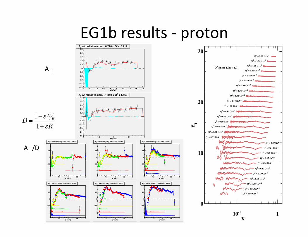
EG1b  results  -­‐  proton  

24

W (GeV)1 1.5 2 2.5 3

-1

-0.5

0

0.5

1 < 0.1562), 0.077 < Q

3/D: electron(NH||A

W (GeV)1 1.5 2 2.5 3

-1

-0.5

0

0.5

1 < 0.3172), 0.156 < Q

3/D: electron(NH||A

W (GeV)1 1.5 2 2.5 3

-1

-0.5

0

0.5

1 < 0.6452), 0.317 < Q

3/D: electron(NH||A

W (GeV)1 1.5 2 2.5 3

-1

-0.5

0

0.5

1 < 1.3102), 0.645 < Q

3/D: electron(NH||A

W (GeV)1 1.5 2 2.5 3

-1

-0.5

0

0.5

1 < 2.6602), 1.310 < Q

3/D: electron(NH||A

W (GeV)1 1.5 2 2.5 3

-1

-0.5

0

0.5

1 < 5.4002), 2.660 < Q

3/D: electron(NH||A

FIG. 33: [Color online] Values of A!/D for each beam en-ergy, including systematic uncertainties. Di!erent shadings(colors) correspond to di!erent beam energies contributing tothe same (W,Q2) bin.

B. Extraction of polarized asymmetries and structurefunctions

The asymmetries A1(Q2, W ) and A2(Q2, W ) are linearlyrelated to A!(Q

2, W ) by Eq. 18. The kinematical depolar-ization factor D in this equation is given in Eq. 14. Thestructure function R was calculated from a fit to the worlddata (see next section). For each final set discussed in theprevious section, the values of A!/D = A1 + !A2 werecalculated for each bin. For sets with beam energies di!er-ing by less than 15%, these values for A!/D were combined(with statistical weighting) and the corresponding beam en-ergies averaged (Figure 33).

Over a large kinematic region, the same (Q2,W ) binswere measured at multiple beam energies. Consequently, forthese bins, A1 and A2 can be obtained from a Rosenbluthtype of separation, see Section II B. For fixed values of Q2

and W A!/D is a linear function of the parameter ! whichdepends on the beam energy. A linear fit in ! determinesboth A1 and A2. The kinematical region where our dataallowed us to apply this method, along with examples of thelinear fits, are shown in Fig. 34. One disadvantage of themethod is its large sensitivity to uncertainties in the dilutionfactor and in PbPt values for di!erent beam energies.

For W < 2 GeV, the model independent results for A2

are shown in Fig. 35, and compared to our model for A2,as well as to RSS data [103] (limited to Q2 = 1.3 GeV2)and data from MIT Bates [104]. and unpublished NIKHEFdata. For these plots bins have been combined to increasethe statistical resolution. Although our results for A2 lackthe precision of the RSS [39] experiment, they extend overa wider range of Q2.

For W > 2 GeV, we rarely have more than two beamenergies contributing to any given kinematic points, andusually only the highest two beam energies. This yields arather poor lever arm in ! and makes any check of the linearfit (as well as its error) impossible. For this reason, we donot quote any results for A2 in the DIS region.

η0.6 0.7 0.8 0.9 1 1.1

/D ||A

-1

-0.8

-0.6

-0.4

-0.2

-0

0.2

0.4

0.6

0.8

1 bin = 252W bin = 121, Q bin = 252W bin = 121, Q

FIG. 34: Approximate kinematic coverage of the linear re-gression method (top-replace with actual data later). Thelinear fit is shown for one sample bin.

The spin structure function g2

A model-independent value of g2 can be obtained if oneexpresses A! directly as a linear combination of g1 andg2, again with energy dependent coe"cients and a modelfor the unpolarized structure function F1; see Eq. 15. For(Q2, W ) bins measured at more than one energy, g1 and g2

can then be determined with a straight-line fit along witha straight-forward calculation of the statistical uncertainty.As already discussed, this is not the best way to determineg1, but it does provide model independent values for g2.The results for the product xg2 averaged over four di!erentQ2 ranges are displayed as functions of x in Fig. 36. Whilethe precision is not particularly good, some constraint onmodels of g2 is provided.

C. Models

To extract high–precision observables of interest from ourdata on A||, we need to use models for the unmeasuredstructure functions F1 and F2 (or, equivalently, F1 and R),as well as for the asymmetry A2 which is only poorly deter-mined by our own data (see above). Using these models, wecan extract A1 and g1 from the measured A||, as explainedin Section II B. In addition, we also need a model for A1

23

Systematic uncertainty Max. Relative Magnitude (g1/F1)

1.6 GeV 2.5 GeV 4.2 GeV 5.7 GeV

Kinematic smearing/uncertainties 2.0% 1.5% 1.0% 0.5%

Target material tolerances 2.5% 2.5% 2.5% 2.5%

DIS ranges used 1.5% 1.5% 1.5% 1.5%

to determine L, !A

Unpolarized cross-section model 4.5% 2.0% 2.0% 2.0%

used to determine FDF

Elastic ep event selection 1.5% 1.5% 1.5% 1.5%

for PbPt analysis

Statistical PbPt uncertainty 0.8% 1.1% 1.7% 2.2%

"! contamination 0.1% 0.8% 0.8% 1.5%

e+e! contamination 1.0% 1.0% 1.0% 1.0%15N polarization 0.5% 0.5% 0.5% 0.5%

Model uncertainties (F2,R,A1,A2) 2.0% 2.0% 2.0% 2.0%

TABLE I: Table of Systematic Error Magnitudes

V. RESULTS AND COMPARISON TO THEORY

A. Extraction of A"

The raw double-spin asymmetry (Eq. 46) was evaluatedfor each group of data with given beam energy, torus po-larity, direction of the target polarization, and status of theHWP (in/out). For each group the raw data were com-bined in (W, Q2) bins. For all energies and W values, thebin width in W was chosen to be !W = 10 MeV. TheQ2 bins were defined logarithmically, with 13 bins in eachdecade of Q2. These bin sizes were chosen to provide acompromise between statistical significance and expectedstructure in the asymmetries.

The data in the various groups were combined accordingto the following procedure. First, for each beam energy andtarget and torus polarity, the raw asymmetries obtained withopposite half-wave-plate (HWP) status were combined, binby bin, weighting the data in each bin according to their sta-tistical uncertainty. Next, the data sets with opposite targetpolarizations were combined using the product !2

A(PbPt)2relas weight to optimize the statistical precision of the result.Here, !A is the statistical uncertainty of the raw asymmetryand (PbPt)rel is a quantity proportional to the product ofbeam and target polarization for a given data set. To getthe highest possible statistical precision for this quantity, wecalculated it by using not only elastic (exclusive) scatteringdata (c.f. Section IV E 2 ), but by taking the ratio of themeasured raw asymmetry to that predicted by our model(see Section VC) for all kinematic bins (including elasticscattering) and averaging over the entire data set. The re-sulting value for (PbPt)rel deviates from the “true” productof polarizations by a constant scale factor which is the samefor the two data sets with opposite target polarization andtherefore plays no role for the purpose of deriving a relative

weight for these two sets.

W (GeV)1 1.1 1.2 1.3 1.4 1.5 1.6 1.7 1.8-0.5

-0.4

-0.3

-0.2

-0.1

-0

0.1

0.2

0.3

0.4

0.5 < 0.3792 w/ radiative corr. , 0.317 < Q||A

W (GeV)1 1.2 1.4 1.6 1.8 2 2.2-0.5

-0.4

-0.3

-0.2

-0.1

-0

0.1

0.2

0.3

0.4

0.5 < 0.5402 w/ radiative corr. , 0.452 < Q||A

W (GeV)1 1.2 1.4 1.6 1.8 2 2.2 2.4 2.6 2.8-0.5

-0.4

-0.3

-0.2

-0.1

-0

0.1

0.2

0.3

0.4

0.5 < 0.9192 w/ radiative corr. , 0.770 < Q||A

W (GeV)1 1.5 2 2.5 3-0.5

-0.4

-0.3

-0.2

-0.1

-0

0.1

0.2

0.3

0.4

0.5 < 1.5602 w/ radiative corr. , 1.310 < Q||A

FIG. 32: Values of A" shown at 1.606 GeV, 2.286 GeV, 4.238GeV, and 5.725 GeV respectively, with radiative correctionsshaded The red curve comes from our model, as discussed inthe text.

All corrections except radiative corrections were then ap-plied for the combined sets. Next, the asymmetries fromsets with opposite torus polarity (but identical beam en-ergy) were averaged (again weighted by statistical uncer-tainty). Finally, radiative corrections, described in SectionIVE 4 were applied, resulting in measurements of A! foreach beam energy (see Figure 32).

x-110 1

1g

0

10

20

30

Shift: 1.0n + 1.02Q

2 = 0.05 GeV2Q

2 = 0.06 GeV2Q

2 = 0.07 GeV2Q

2 = 0.08 GeV2Q

2 = 0.10 GeV2Q

2 = 0.12 GeV2Q

2 = 0.14 GeV2Q

2 = 0.17 GeV2Q

2 = 0.20 GeV2Q

2 = 0.24 GeV2Q

2 = 0.29 GeV2Q

2 = 0.35 GeV2Q

2 = 0.41 GeV2Q

2 = 0.49 GeV2Q

2 = 0.59 GeV2Q

2 = 0.70 GeV2Q

2 = 0.84 GeV2Q

2 = 1.00 GeV2Q

2 = 1.19 GeV2Q

2 = 1.42 GeV2Q

2 = 1.70 GeV2Q

2 = 2.03 GeV2Q

2 = 2.42 GeV2Q

2 = 2.88 GeV2Q

2 = 3.42 GeV2Q

2 = 4.06 GeV2Q

2 = 4.87 GeV2Q

2 = 5.66 GeV2Q

A||  

A||/D  

D =1−ε E '

E

1+εR

A||/D  for  the  Deuteron