p 6= np - faculteit wiskunde en informaticagwoegi/p-versus-np/deolalikar.pdf · abstract we...
TRANSCRIPT

Abstract
We demonstrate the separation of the complexity class NP from its subclass P. Throughoutour proof, we observe that the ability to compute a property on structures in polynomial time isintimately related to the statistical notions of conditional independence and sufficient statistics.The presence of conditional independencies manifests in the form of economical parametriza-tions of the joint distribution of covariates. In order to apply this analysis to the space of so-lutions of random constraint satisfaction problems, we utilize and expand upon ideas fromseveral fields spanning logic, statistics, graphical models, random ensembles, and statisticalphysics.
We begin by introducing the requisite framework of graphical models for a set of interactingvariables. We focus on the correspondence between Markov and Gibbs properties for directedand undirected models as reflected in the factorization of their joint distribution, and the num-ber of independent parameters required to specify the distribution.
Next, we build the central contribution of this work. We show that there are fundamentalconceptual relationships between polynomial time computation, which is completely capturedby the logic FO(LFP) on some classes of structures, and certain directed Markov propertiesstated in terms of conditional independence and sufficient statistics. In order to demonstratethese relationships, we view a LFP computation as “factoring through” several stages of firstorder computations, and then utilize the limitations of first order logic. Specifically, we exploitthe limitation that first order logic can only express properties in terms of a bounded numberof local neighborhoods of the underlying structure.
Next we introduce ideas from the 1RSB replica symmetry breaking ansatz of statisticalphysics. We recollect the description of the d1RSB clustered phase for random k-SAT thatarises when the clause density is sufficiently high. In this phase, an arbitrarily large fractionof all variables in cores freeze within exponentially many clusters in the thermodynamic limit,as the clause density is increased towards the SAT-unSAT threshold for large enough k. TheHamming distance between a solution that lies in one cluster and that in another is O(n).
Next, we encode k-SAT formulae as structures on which FO(LFP) captures polynomial time.By asking FO(LFP) to extend partial assignments on ensembles of random k-SAT, we build dis-tributions of solutions. We then construct a dynamic graphical model on a product space thatcaptures all the information flows through the various stages of a LFP computation on ensem-bles of k-SAT structures. Distributions computed by LFP must satisfy this model. This modelis directed, which allows us to compute factorizations locally and parameterize using Gibbspotentials on cliques. We then use results from ensembles of factor graphs of random k-SATto bound the various information flows in this directed graphical model. We parametrize theresulting distributions in a manner that demonstrates that irreducible interactions between co-variates — namely, those that may not be factored any further through conditional independen-cies — cannot grow faster than poly(log n) in the LFP computed distributions. This character-ization allows us to analyze the behavior of the entire class of polynomial time algorithms onensembles simultaneously.
Using the aforementioned limitations of LFP, we demonstrate that a purported polynomialtime solution to k-SAT would result in solution space that is a mixture of distributions eachhaving an exponentially smaller parametrization than is consistent with the highly constrainedd1RSB phases of k-SAT. We show that this would contradict the behavior exhibited by the so-lution space in the d1RSB phase. This corresponds to the intuitive picture provided by physicsabout the emergence of extensive (meaning O(n)) long-range correlations between variables in

this phase and also explains the empirical observation that all known polynomial time algo-rithms break down in this phase.
Our work shows that every polynomial time algorithm must fail to produce solutions tolarge enough problem instances of k-SAT in the d1RSB phase. This shows that polynomialtime algorithms are not capable of solving NP-complete problems in their hard phases, anddemonstrates the separation of P from NP.

Contents
1 Introduction 31.1 Synopsis of Proof . . . . . . . . . . . . . . . . . . . . . . . . . . . . . . . . . . . . . 4
2 Interaction Models and Conditional Independence 92.1 Conditional Independence . . . . . . . . . . . . . . . . . . . . . . . . . . . . . . . . 92.2 Conditional Independence in Undirected Graphical Models . . . . . . . . . . . . 10
2.2.1 Gibbs Random Fields and the Hammersley-Clifford Theorem . . . . . . . 132.3 Factor Graphs . . . . . . . . . . . . . . . . . . . . . . . . . . . . . . . . . . . . . . . 142.4 The Markov-Gibbs Correspondence for Directed Models . . . . . . . . . . . . . . 152.5 I-maps and D-maps . . . . . . . . . . . . . . . . . . . . . . . . . . . . . . . . . . . 172.6 Parametrization . . . . . . . . . . . . . . . . . . . . . . . . . . . . . . . . . . . . . . 18
3 Logical Descriptions of Computations 203.1 Inductive Definitions and Fixed Points . . . . . . . . . . . . . . . . . . . . . . . . . 203.2 Fixed Point Logics for P and PSPACE . . . . . . . . . . . . . . . . . . . . . . . . 22
4 The Link Between Polynomial Time Computation and Conditional Independence 254.1 The Limitations of LFP . . . . . . . . . . . . . . . . . . . . . . . . . . . . . . . . . . 26
4.1.1 Locality of First Order Logic . . . . . . . . . . . . . . . . . . . . . . . . . . 264.2 Simple Monadic LFP and Conditional Independence . . . . . . . . . . . . . . . . 294.3 Conditional Independence in Complex Fixed Points . . . . . . . . . . . . . . . . . 324.4 Aggregate Properties of LFP over Ensembles . . . . . . . . . . . . . . . . . . . . . 32
5 The 1RSB Ansatz of Statistical Physics 345.1 Ensembles and Phase Transitions . . . . . . . . . . . . . . . . . . . . . . . . . . . . 345.2 The d1RSB Phase . . . . . . . . . . . . . . . . . . . . . . . . . . . . . . . . . . . . . 35
5.2.1 Cores and Frozen Variables . . . . . . . . . . . . . . . . . . . . . . . . . . . 365.2.2 Performance of Known Algorithms . . . . . . . . . . . . . . . . . . . . . . 38
6 Random Graph Ensembles 396.1 Properties of Factor Graph Ensembles . . . . . . . . . . . . . . . . . . . . . . . . . 39
6.1.1 Locally Tree-Like Property . . . . . . . . . . . . . . . . . . . . . . . . . . . 396.1.2 Degree Profiles in Random Graphs . . . . . . . . . . . . . . . . . . . . . . . 40
7 Separation of Complexity Classes 427.1 Measuring Conditional Independence . . . . . . . . . . . . . . . . . . . . . . . . . 427.2 Generating Distributions from LFP . . . . . . . . . . . . . . . . . . . . . . . . . . . 43
7.2.1 Encoding k-SAT into Structures . . . . . . . . . . . . . . . . . . . . . . . . 43
1

2
7.2.2 The LFP Neighborhood System . . . . . . . . . . . . . . . . . . . . . . . . . 447.2.3 Generating Distributions . . . . . . . . . . . . . . . . . . . . . . . . . . . . 45
7.3 Disentangling the Interactions: The ENSP Model . . . . . . . . . . . . . . . . . . . 467.4 Parametrization of the ENSP . . . . . . . . . . . . . . . . . . . . . . . . . . . . . . . 507.5 Separation . . . . . . . . . . . . . . . . . . . . . . . . . . . . . . . . . . . . . . . . . 527.6 Some Perspectives . . . . . . . . . . . . . . . . . . . . . . . . . . . . . . . . . . . . . 54
A Reduction to a Single LFP Operation 56A.1 The Transitivity Theorem for LFP . . . . . . . . . . . . . . . . . . . . . . . . . . . . 56A.2 Sections and the Simultaneous Induction Lemma for LFP . . . . . . . . . . . . . . 56
2

1. Introduction
The P?= NP question is generally considered one of the most important and far reaching
questions in contemporary mathematics and computer science.The origin of the question seems to date back to a letter from Godel to Von Neumann in
1956 [Sip92]. Formal definitions of the class NP awaited work by Edmonds [Edm65], Cook[Coo71], and Levin [Lev73]. The Cook-Levin theorem showed the existence of complete prob-lems for this class, and demonstrated that SAT– the problem of determining whether a set ofclauses of Boolean literals has a satisfying assignment – was one such problem. Later, Karp[Kar72] showed that twenty-one well known combinatorial problems, which include TRAV-ELLING SALESMAN, CLIQUE, and HAMILTONIAN CIRCUIT, were also NP-complete. In subse-quent years, many problems central to diverse areas of application were shown to be NP-complete(see [GJ79] for a list). If P 6= NP, we could never solve these problems efficiently. If, on theother hand P = NP, the consequences would be even more stunning, since every one of theseproblems would have a polynomial time solution. The implications of this on applications suchas cryptography, and on the general philosophical question of whether human creativity can beautomated, would be profound.
The P?= NP question is also singular in the number of approaches that researchers have
brought to bear upon it over the years. From the initial question in logic, the focus moved tocomplexity theory where early work used diagonalization and relativization techniques. How-
ever, [BGS75] showed that these methods were perhaps inadequate to resolve P?= NP by
demonstrating relativized worlds in which P = NP and others in which P 6= NP (both re-lations for the appropriately relativized classes). This shifted the focus to methods using cir-cuit complexity and for a while this approach was deemed the one most likely to resolve thequestion. Once again, a negative result in [RR97] showed that a class of techniques known as“Natural Proofs” that subsumed the above could not separate the classes NP and P, providedone-way functions exist.
Owing to the difficulty of resolving the question, and also to the negative results mentioned
above, there has been speculation that resolving the P?= NP question might be outside the
domain of mathematical techniques. More precisely, the question might be independent ofstandard axioms of set theory. The first such results in [HH76] show that some relativized
versions of the P?= NP question are independent of reasonable formalizations of set theory.
The influence of the P?= NP question is felt in other areas of mathematics. We mention
one of these, since it is central to our work. This is the area of descriptive complexity theory— the branch of finite model theory that studies the expressive power of various logics viewedthrough the lens of complexity theory. This field began with the result [Fag74] that showedthat NP corresponds to queries that are expressible in second order existential logic over fi-nite structures. Later, characterizations of the classes P [Imm86], [Var82] and PSPACE overordered structures were also obtained.
There are several introductions to the P?= NP question and the enormous amount of re-
3

1. INTRODUCTION 4
search that it has produced. The reader is referred to [Coo06] for an introduction which alsoserves as the official problem description for the Clay Millenium Prize. An older excellent re-view is [Sip92]. See [Wig07] for a more recent introduction. Most books on theoretical computerscience in general, and complexity theory in particular, also contain accounts of the problem andattempts made to resolve it. See the books [Sip96] and [BDG95] for standard references.
Preliminaries and Notation
Treatments of standard notions from complexity theory, such as definitions of the complexityclasses P, NP, PSPACE, and notions of reductions and completeness for complexity classes,etc. may be found in [Sip96, BDG95].
Our work will span various developments in three broad areas. While we have endeavoredto be relatively complete in our treatment, we feel it would be helpful to provide standardtextual references for these areas, in the order in which they appear in the work. Additionalreferences to results will be provided within the chapters.
Standard references for graphical models include [Lau96] and the more recent [KF09]. For anengaging introduction, please see [Bis06, Ch. 8]. For an early treatment in statistical mechanicsof Markov random fields and Gibbs distributions, see [KS80].
Preliminaries from logic, such as notions of structure, vocabulary, first order language, mod-els, etc., may be obtained from any standard text on logic such as [Hod93]. In particular, we re-fer to [EF06, Lib04] for excellent treatments of finite model theory and [Imm99] for descriptivecomplexity.
For a treatment of the statistical physics approach to random CSPs, we recommend [MM09].An earlier text is [MPV87].
1.1 Synopsis of Proof
This proof requires a convergence of ideas and an interplay of principles that span several areaswithin mathematics and physics. This represents the majority of the effort that went into con-structing the proof. Given this, we felt that it would be beneficial to explain the various stagesof the proof, and highlight their interplay. The technical details of each stage are described insubsequent chapters.
Consider a system of n interacting variables such as is ubiquitous in mathematical sciences.For example, these may be the variables in a k-SAT instance that interact with each otherthrough the clauses present in the k-SAT formula, or n Ising spins that interact with each otherin a ferromagnet. Through their interaction, variables exert an influence on each other, and af-fect the values each other may take. The proof centers on the study of logical and algorithmicconstructs where such complex interactions factor into “simpler” ones.
The factorization of interactions can be represented by a corresponding factorization of thejoint distribution of the variables over the space of configurations of the n variables subject tothe constraints of the problem. It has been realized in the statistics and physics communities forlong that certain multivariate distributions decompose into the product of a few types of factors,with each factor itself having only a few variables. Such a factorization of joint distributions intosimpler factors can often be represented by graphical models whose vertices index the variables.A factorization of the joint distribution according to the graph implies that the interactionsbetween variables can be factored into a sequence of “local interactions” between vertices thatlie within neighborhoods of each other.
4

1. INTRODUCTION 5
Consider the case of an undirected graphical model. The factoring of interactions may bestated in terms of either a Markov property, or a Gibbs property with respect to the graph.Specifically, the local Markov property of such models states that the distribution of a variableis only dependent directly on that of its neighbors in an appropriate neighborhood system. Ofcourse, two variables arbitrarily far apart can influence each other, but only through a sequence ofsuccessive local interactions. The global Markov property for such models states that when two setsof vertices are separated by a third, this induces a conditional independence on variables corre-sponding to these sets of vertices, given those corresponding to the third set. On the other hand,the Gibbs property of a distribution with respect to a graph asserts that the distribution factorsinto a product of potential functions over the maximal cliques of the graph. Each potential cap-tures the interaction between the set of variables that form the clique. The Hammersley-Cliffordtheorem states that a positive distribution having the Markov property with respect to a graphmust have the Gibbs property with respect to the same graph.
The condition of positivity is essential in the Hammersley-Clifford theorem for undirectedgraphs. However, it is not required when the distribution satisfies certain directed models. Inthat case, the Markov property with respect to the directed graph implies that the distributionfactorizes into local conditional probability distributions (CPDs). Furthermore, if the model is adirected acyclic graph (DAG), we can obtain the Gibbs property with respect to an undirectedgraph constructed from the DAG by a process known as moralization. We will return to thedirected case shortly.
At this point we begin to see that factorization into conditionally independent pieces man-ifests in terms of economical parametrizations of the joint distribution. Thus, the number ofindependent parameters required to specify the joint distribution may be used as a measure ofthe complexity of interactions between the covariates. When the variates are independent, thismeasure takes its least value. Dependencies introduced at random (such as in random k-SAT)cause it to rise. Roughly speaking, this measure is (O(ck), c > 1) where k is the largest interac-tion between the variables that cannot be decomposed any further. Intuitively, we know thatconstraint satisfaction problems (CSPs) are hard when we cannot separate their joint constraintsinto smaller easily manageable pieces. This should be reflected then, in the growth of this mea-sure on the distribution of all solutions to random CSPs as their constraint densities are increased.Informally, a CSP is hard (but satisfiable) when the distribution of all its solutions is complexto describe in terms of its number of independent parameters due to the extensive interactionsbetween the variables in the CSP. Graphical models offer us a way to measure the size of theseinteractions.
Chapter 2 develops the principles underlying the framework of graphical models. We willnot use any of these models in particular, but construct another directed model on a largerproduct space that utilizes these principles and tailors them to the case of least fixed point logic,which we turn to next.
At this point, we change to the setting of finite model theory. Finite model theory is a branchof mathematical logic that has provided machine independent characterizations of various im-portant complexity classes including P, NP, and PSPACE. In particular, the class of polyno-mial time computable queries on ordered structures has a precise description — it is the class ofqueries expressible in the logic FO(LFP) which extends first order logic with the ability to com-pute least fixed points of positive first order formulae. Least fixed point constructions iterate anunderlying positive first order formula, thereby building up a relation in stages. We take a geo-metric picture of a LFP computation. Initially the relation to be built is empty. At the first stage,certain elements, whose types satisfy the first order formula, enter the relation. This changesthe neighborhoods of these elements, and therefore in the next stage, other elements (whoseneighborhoods have been thus changed in the previous stages) become eligible for entering the
5

1. INTRODUCTION 6
relation. The positivity of the formula implies that once an element is in the relation, it cannotbe removed, and so the iterations reach a fixed point in a polynomial number of steps. Impor-tantly from our point of view, the positivity and the stage-wise nature of LFP means that thecomputation has a directed representation on a graphical model that we will construct. Recallat this stage that distributions over directed models enjoy factorization even when they are notdefined over the entire space of configurations.
We may interpret this as follows: LFP relies on the assumption that variables that are highlyentangled with each other due to constraints can be disentangled in a way that they now inter-act with each other through conditional independencies induced by a certain directed graph-ical model construction. Of course, an element does influence others arbitrarily far away, butonly through a sequence of such successive local and bounded interactions. The reason LFP compu-tations terminate in polynomial time is analogous to the notions of conditional independencethat underlie efficient algorithms on graphical models having sufficient factorization into localinteractions.
In order to apply this picture in full generality to all LFP computations, we use the simulta-neous induction lemma to push all simultaneous inductions into nested ones, and then employthe transitivity theorem to encode nested fixed points as sections of a single relation of higherarity. Finally, we either do the extra bookkeeping to work with relations of higher arity, or workin a larger structure where the relation of higher arity is monadic (namely, structures of k-typesof the original structure). Either of these cases presents only a polynomially larger overhead,and does not hamper our proof scheme. Building the machinery that can precisely map all thesecases to the picture of factorization into local interactions is the subject of Chapter 4.
The preceding insights now direct us to the setting necessary in order to separate P fromNP. We need a regime of NP-complete problems where interactions between variables are so“dense” that they cannot be factored through the bottleneck of the local and bounded proper-ties of first order logic that limit each stage of LFP computation. Intuitively, this should happenwhen each variable has to simultaneously satisfy constraints involving an extensive (O(n)) frac-tion of the variables in the problem.
In search of regimes where such situations arise, we turn to the study of ensemble randomk-SAT where the properties of the ensemble are studied as a function of the clause densityparameter. We will now add ideas from this field which lies on the intersection of statisticalmechanics and computer science to the set of ideas in the proof.
In the past two decades, the phase changes in the solution geometry of random k-SATensembles as the clause density increases, have gathered much research attention. The 1RSBansatz of statistical mechanics says that the space of solutions of random k-SAT shatters intoexponentially many clusters of solutions when the clause density is sufficiently high. This phaseis called 1dRSB (1-Step Dynamic Replica Symmetry Breaking) and was conjectured by physi-cists as part of the 1RSB ansatz. It has since been rigorously proved for high values of k. Itdemonstrates the properties of high correlation between large sets of variables that we willneed. Specifically, the emergence of cores that are sets of C clauses all of whose variables lie in aset of size C (this actually forces C to be O(n)). As the clause density is increased, the variablesin these cores “freeze.” Namely, they take the same value throughout the cluster. Changing thevalue of a variable within a cluster necessitates changing O(n) other variables in order to arriveat another satisfying solution, which would be in a different cluster. Furthermore, as the clausedensity is increased towards the SAT-unSAT threshold, each cluster collapses steadily towardsa single solution, that is maximally far apart from every other cluster. Physicists think of this asan “energy gap” between the clusters. Such stages are precisely the ones that cannot be factoredthrough local and bounded first order stages of a LFP computation due to the tight coupling be-tween O(n) variables. Finally, as the clause density increases above the SAT-unSAT threshold,
6

1. INTRODUCTION 7
the solution space vanishes, and the underlying instance of SAT is no longer satisfiable. Wereproduce the rigorously proved picture of the 1RSB ansatz that we will need in Chapter 5.
In Chapter 6, we make a brief excursion into the random graph theory of the factor graphensembles underlying random k-SAT. From here, we obtain results that asymptotically almostsurely upper bound the size of the largest cliques in the neighborhood systems on the Gaifmangraphs that we study later. These provide us with bounds on the largest irreducible interactionsbetween variables during the various stages of an LFP computation.
Finally in Chapter 7, we pull all the threads and machinery together. First, we encode k-SATinstances as queries on structures over a certain vocabulary in a way that LFP captures all poly-nomial time computable queries on them. We then set up the framework whereby we cangenerate distributions of solutions to each instance by asking a purported LFP algorithm fork-SAT to extend partial assignments on variables to full satisfying assignments.
Next, we embed the space of covariates into a larger product space which allows us to “dis-entangle” the flow of information during a LFP computation. This allows us to study thecomputations performed by the LFP with various initial values under a directed graphicalmodel. This model is only polynomially larger than the structure itself. We call this the Element-Neighborhood-Stage Product, or ENSP model. The distribution of solutions generated by LFP thenis a mixture of distributions each of whom factors according to an ENSP.
At this point, we wish to measure the growth of independent parameters of distributions ofsolutions whose embeddings into the larger product space factor over the ENSP. In order to doso, we utilize the following properties.
1. The directed nature of the model that comes from properties of LFP.
2. The properties of neighborhoods that are obtained by studies on random graph ensem-bles, specifically that neighborhoods that occur during the LFP computation are of sizepoly(log n) asymptotically almost surely in the n→∞ limit.
3. The locality and boundedness properties of FO that put constraints upon each individualstage of the LFP computation.
4. Simple properties of LFP, such as the closure ordinal being a polynomial in the structuresize.
The crucial property that allows us to analyze mixtures of distributions that factor accord-ing to some ENSP is that we can parametrize the distribution using potentials on cliques ofits moralized graph that are of size at most poly(log n). This means that when the mixture isexponentially numerous, we will see features that reflect the poly(log n) factor size of the condi-tionally independent parametrization.
Now we close the loop and show that a distribution of solutions for SAT with these proper-ties would contradict the known picture of k-SAT in the d1RSB phase for k > 8 — namely, thepresence of extensive frozen variables in exponentially many clusters with Hamming distancebetween the clusters being O(n). In particular, in exponentially numerous mixtures, we wouldhave conditionally independent variation between blocks of poly(log n) variables, causing theHamming distance between solutions to be of this order as well. In other words, solutions fork-SAT that are constructed using LFP will display aggregate behavior that reflects that theyare constructed out of “building blocks” of size poly(log n). This behavior will manifest whenexponentially many solutions are generated by the LFP construction.
This shows that LFP cannot express the satisfiability query in the d1RSB phase for highenough k, and separates P from NP. This also explains the empirical observation that all
7

1. INTRODUCTION 8
known polynomial time algorithms fail in the d1RSB phase for high values of k, and also es-tablishes on rigorous principles the physics intuition about the onset of extensive long rangecorrelations in the d1RSB phase that causes all known polynomial time algorithms to fail.
8
2. Interaction Models andConditional Independence
Systems involving a large number of variables interacting in complex ways are ubiquitous inthe mathematical sciences. These interactions induce dependencies between the variables. Be-cause of the presence of such dependencies in a complex system with interacting variables, itis not often that one encounters independence between variables. However, one frequently en-counters conditional independence between sets of variables. Both independence and conditionalindependence among sets of variables have been standard objects of study in probability andstatistics. Speaking in terms of algorithmic complexity, one often hopes that by exploiting theconditional independence between certain sets of variables, one may avoid the cost of enumer-ation of an exponential number of hypothesis in evaluating functions of the distribution thatare of interest.
2.1 Conditional Independence
We first fix some notation. Random variables will be denoted by upper case letters such asX,Y, Z, etc. The values a random variable takes will be denoted by the corresponding lowercase letters, such as x, y, z. Throughout this work, we assume our random variables to be dis-crete unless stated otherwise. We may also assume that they take values in a common finitestate space, which we usually denote by Λ following physics convention. We denote the proba-bility mass functions of discrete random variables X,Y, Z by PX(x), PY (y), PZ(z) respectively.Similarly, PX,Y (x, y) will denote the joint mass of (X,Y ), and so on. We drop subscripts on theP when it causes no confusion. We freely use the term “distribution” for the probability massfunction.
The notion of conditional independence is central to our proof. The intuitive definition ofthe conditional independence of X from Y given Z is that the conditional distribution of Xgiven (Y,Z) is equal to the conditional distribution of X given Z alone. This means that oncethe value of Z is given, no further information about the value of X can be extracted from thevalue of Y . This is an asymmetric definition, and can be replaced by the following symmetricdefinition. Recall that X is independent of Y if
P (x, y) = P (x)P (y).
Definition 2.1. Let notation be as above. X is conditionally independent of Y given Z, writtenX⊥⊥Y |Z, if
P (x, y | z) = P (x | z)P (y | z),
9

2. INTERACTION MODELS AND CONDITIONAL INDEPENDENCE 10
The asymmetric version which says that the information contained in Y is superfluous todetermining the value of X once the value of Z is known may be represented as
P (xcondy, z) = P (x | z).
The notion of conditional independence pervades statistical theory [Daw79, Daw80]. Sev-eral notions from statistics may be recast in this language.
EXAMPLE 2.2. The notion of sufficiency may be seen as the presence of a certain conditionalindependence [Daw79]. A sufficient statistic T in the problem of parameter estimation is thatwhich renders the estimate of the parameter independent of any further information from thesample X . Thus, if Θ is the parameter to be estimated, then T is a sufficient statistic if
P (θ |x) = P (θ | t).
Thus, all there is to be gained from the sample in terms of information about Θ is already presentin T alone. In particular, if Θ is a posterior that is being computed by Bayesian inference, thenthe above relation says that the posterior depends on the data X through the value of T alone.Clearly, such a statement would lead to a reduction in the complexity of inference.
2.2 Conditional Independence in Undirected Graphical Mod-els
Graphical models offer a convenient framework and methodology to describe and exploit con-ditional independence between sets of variables in a system. One may think of the graphicalmodel as representing the family of distributions whose law fulfills the conditional indepen-dence statements made by the graph. A member of this family may satisfy any number of ad-ditional conditional independence statements, but not less than those prescribed by the graph.In general, we will consider graphs G = (V,E) whose n vertices index a set of n random vari-ables (X1, . . . , Xn). The random variables all take their values in a common state space Λ. Therandom vector (X1, . . . , Xn) then takes values in a configuration space Ωn = Λn. We will denotevalues of the random vector (X1, . . . , Xn) simply by x = (x1, . . . , xn). The notation XV \I willdenote the set of variables excluding those whose indices lie in the set I . Let P be a probabilitymeasure on the configuration space. We will study the interplay between conditional indepen-dence properties of P and its factorization properties.
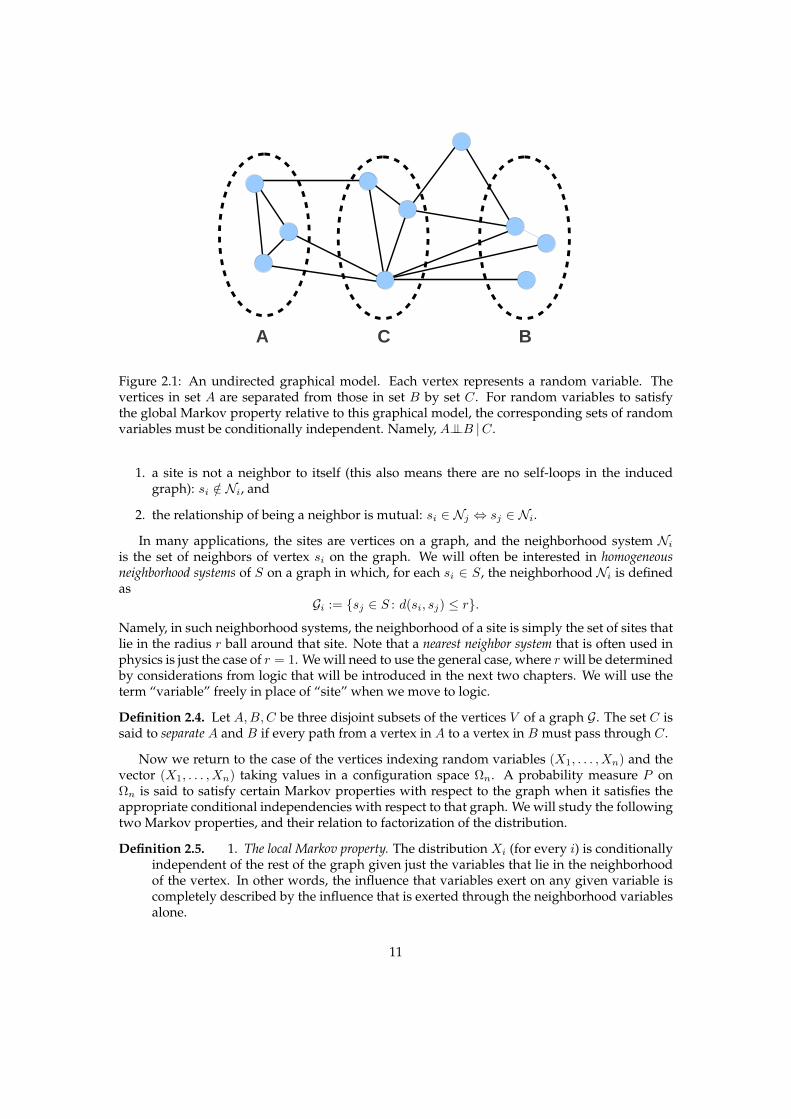
There are, broadly, two kinds of graphical models: directed and undirected. We first con-sider the case of undirected models. Fig. 2.1 illustrates an undirected graphical model with tenvariables.
Random Fields and Markov Properties
Graphical models are very useful because they allow us to read off conditional independenciesof the distributions that satisfy these models from the graph itself. Recall that we wish to studythe relation between conditional independence of a distribution with respect to a graphicalmodel, and its factorization. Towards that end, one may write increasingly stringent condi-tional independence properties that a set of random variables satisfying a graphical model maypossess, with respect to the graph. In order to state these, we first define two graph theoreticnotions — those of a general neighborhood system, and of separation.
Definition 2.3. Given a set of variables S known as sites, a neighborhood system NS on S is acollection of subsets Ni : 1 ≤ i ≤ n indexed by the sites in S that satisfy
10
2. INTERACTION MODELS AND CONDITIONAL INDEPENDENCE 11
A C B
Figure 2.1: An undirected graphical model. Each vertex represents a random variable. Thevertices in set A are separated from those in set B by set C. For random variables to satisfythe global Markov property relative to this graphical model, the corresponding sets of randomvariables must be conditionally independent. Namely, A⊥⊥B |C.
1. a site is not a neighbor to itself (this also means there are no self-loops in the inducedgraph): si /∈ Ni, and
2. the relationship of being a neighbor is mutual: si ∈ Nj ⇔ sj ∈ Ni.
In many applications, the sites are vertices on a graph, and the neighborhood system Niis the set of neighbors of vertex si on the graph. We will often be interested in homogeneousneighborhood systems of S on a graph in which, for each si ∈ S, the neighborhood Ni is definedas
Gi := sj ∈ S : d(si, sj) ≤ r.
Namely, in such neighborhood systems, the neighborhood of a site is simply the set of sites thatlie in the radius r ball around that site. Note that a nearest neighbor system that is often used inphysics is just the case of r = 1. We will need to use the general case, where r will be determinedby considerations from logic that will be introduced in the next two chapters. We will use theterm “variable” freely in place of “site” when we move to logic.
Definition 2.4. Let A,B,C be three disjoint subsets of the vertices V of a graph G. The set C issaid to separate A and B if every path from a vertex in A to a vertex in B must pass through C.
Now we return to the case of the vertices indexing random variables (X1, . . . , Xn) and thevector (X1, . . . , Xn) taking values in a configuration space Ωn. A probability measure P onΩn is said to satisfy certain Markov properties with respect to the graph when it satisfies theappropriate conditional independencies with respect to that graph. We will study the followingtwo Markov properties, and their relation to factorization of the distribution.
Definition 2.5. 1. The local Markov property. The distribution Xi (for every i) is conditionallyindependent of the rest of the graph given just the variables that lie in the neighborhoodof the vertex. In other words, the influence that variables exert on any given variable iscompletely described by the influence that is exerted through the neighborhood variablesalone.
11
2. INTERACTION MODELS AND CONDITIONAL INDEPENDENCE 12
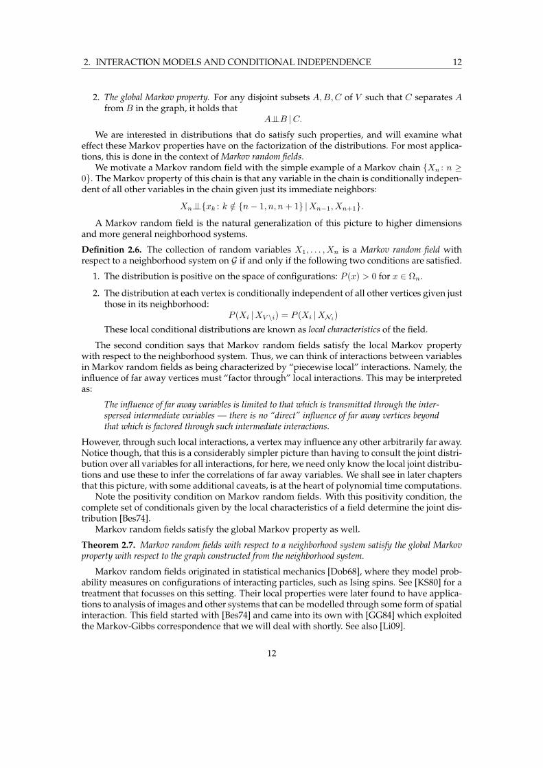
2. The global Markov property. For any disjoint subsets A,B,C of V such that C separates Afrom B in the graph, it holds that
A⊥⊥B |C.
We are interested in distributions that do satisfy such properties, and will examine whateffect these Markov properties have on the factorization of the distributions. For most applica-tions, this is done in the context of Markov random fields.
We motivate a Markov random field with the simple example of a Markov chain Xn : n ≥0. The Markov property of this chain is that any variable in the chain is conditionally indepen-dent of all other variables in the chain given just its immediate neighbors:
Xn⊥⊥xk : k /∈ n− 1, n, n+ 1 |Xn−1, Xn+1.
A Markov random field is the natural generalization of this picture to higher dimensionsand more general neighborhood systems.
Definition 2.6. The collection of random variables X1, . . . , Xn is a Markov random field withrespect to a neighborhood system on G if and only if the following two conditions are satisfied.
1. The distribution is positive on the space of configurations: P (x) > 0 for x ∈ Ωn.
2. The distribution at each vertex is conditionally independent of all other vertices given justthose in its neighborhood:
P (Xi |XV \i) = P (Xi |XNi)
These local conditional distributions are known as local characteristics of the field.
The second condition says that Markov random fields satisfy the local Markov propertywith respect to the neighborhood system. Thus, we can think of interactions between variablesin Markov random fields as being characterized by “piecewise local” interactions. Namely, theinfluence of far away vertices must “factor through” local interactions. This may be interpretedas:
The influence of far away variables is limited to that which is transmitted through the inter-spersed intermediate variables — there is no “direct” influence of far away vertices beyondthat which is factored through such intermediate interactions.
However, through such local interactions, a vertex may influence any other arbitrarily far away.Notice though, that this is a considerably simpler picture than having to consult the joint distri-bution over all variables for all interactions, for here, we need only know the local joint distribu-tions and use these to infer the correlations of far away variables. We shall see in later chaptersthat this picture, with some additional caveats, is at the heart of polynomial time computations.
Note the positivity condition on Markov random fields. With this positivity condition, thecomplete set of conditionals given by the local characteristics of a field determine the joint dis-tribution [Bes74].
Markov random fields satisfy the global Markov property as well.
Theorem 2.7. Markov random fields with respect to a neighborhood system satisfy the global Markovproperty with respect to the graph constructed from the neighborhood system.
Markov random fields originated in statistical mechanics [Dob68], where they model prob-ability measures on configurations of interacting particles, such as Ising spins. See [KS80] for atreatment that focusses on this setting. Their local properties were later found to have applica-tions to analysis of images and other systems that can be modelled through some form of spatialinteraction. This field started with [Bes74] and came into its own with [GG84] which exploitedthe Markov-Gibbs correspondence that we will deal with shortly. See also [Li09].
12

2. INTERACTION MODELS AND CONDITIONAL INDEPENDENCE 13
2.2.1 Gibbs Random Fields and the Hammersley-Clifford Theorem
We are interested in how the Markov properties of the previous section translate into factoriza-tion of the distribution. Note that Markov random fields are characterized by a local condition— namely, their local conditional independence characteristics. We now describe another ran-dom field that has a global characterization — the Gibbs random field.
Definition 2.8. A Gibbs random field (or Gibbs distribution) with respect to a neighborhood systemNG on the graph G is a probability measure on the set of configurations Ωn having a represen-tation of the form
P (x1, . . . , xn) =1
Zexp(−U(x)
T),
where
1. Z is the partition function and is a normalizing factor that ensures that the measure sumsto unity,
Z =∑x∈Ωn
exp(−U(x)
T).
Evaluating Z explicitly is hard in general since it is a summation over each of the Λn
configurations in the space.
2. T is a constant known as the “Temperature” that has origins in statistical mechanics. Itcontrols the sharpness of the distribution. At high temperatures, the distribution tends tobe uniform over the configurations. At low temperatures, it tends towards a distributionthat is supported only on the lowest energy states.
3. U(x) is the “energy” of configuration x and takes the following form as a sum
U(x) =∑c∈C
Vc(x).
over the set of cliques C of G. The functions Vc : c ∈ C are the clique potentials such that thevalue of Vc(x) depends only on the coordinates of x that lie in the clique c. These capturethe interactions between vertices in the clique.
Thus, a Gibbs random field has a probability distribution that factorizes into its constituent“interaction potentials.” This says that the probability of a configuration depends only on theinteractions that occur between the variables, broken up into cliques. For example, let us saythat in a system, each particle interacts with only 2 other particles at a time, (if one prefers tothink in terms of statistical mechanics) then the energy of each state would be expressible as asum of potentials, each of whom had just three variables in its support. Thus, the Gibbs factor-ization carries in it a faithful representation of the underlying interactions between the particles.This type of factorization obviously yields a “simpler description” of the distribution. The pre-cise notion is that of independent parameters it takes to specify the distribution. Factorization intoconditionally independent interactions of scope k means that we can specify the distribution inO(γk) parameters rather than O(γn). We will return to this at the end of this chapter.
Definition 2.9. Let P be a Gibbs distribution whose energy function U(x) =∑c∈C Vc(x). The
support of the potential Vc is the cardinality of the clique c. The degree of the distribution P ,denoted by deg(P ), is the maximum of the supports of the potentials. In other words, thedegree of the distribution is the size of the largest clique that occurs in its factorization.
13
2. INTERACTION MODELS AND CONDITIONAL INDEPENDENCE 14
One may immediately see that the degree of a distribution is a measure of the complexityof interactions in the system since it is the size of the largest set of variables whose interactioncannot be split up in terms of smaller interactions between subsets. One would expect this tobe the hurdle in efficient algorithmic applications.
The Hammersley-Clifford theorem relates the two types of random fields.
Theorem 2.10 (Hammersley-Clifford). X is Markov random field with respect to a neighborhoodsystem NG on the graph G if and only if it is a Gibbs random field with respect to the same neighborhoodsystem.
The theorem appears in the unpublished manuscript [HC71] and uses a certain “blackeningalgebra” in the proof. The first published proofs appear in [Bes74] and [Mou74].
Note that the condition of positivity on the distribution (which is part of the definition of aMarkov random field) is essential to state the theorem in full generality. The following examplefrom [Mou74] shows that relaxing this condition allows us to build distributions having theMarkov property, but not the Gibbs property.
EXAMPLE 2.11. Consider a system of four binary variables X1, X2, X3, X4. Each of the fol-lowing combinations have probability 1/8, while the remaining combinations are disallowed.
(0, 0, 0, 0) (1, 0, 0, 0) (1, 1, 0, 0) (1, 1, 1, 0)
(0, 0, 0, 1) (0, 0, 1, 1) (0, 1, 1, 1) (1, 1, 1, 1).
We may check that this distribution has the global Markov property with respect to the 4 vertexcycle graph. Namely we have
X1⊥⊥X3 |X2, X4 and X2⊥⊥X4 |X1, X3.
However, the distribution does not factorize into Gibbs potentials.
2.3 Factor Graphs
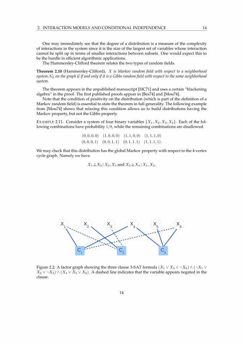
Factor graphs are bipartite graphs that express the decomposition of a “global” multivariatefunction into “local” functions of subsets of the set of variables. They are a class of undirectedmodels. The two types of nodes in a factor graph correspond to variable nodes, and factornodes. See Fig. 2.2.
x1
C1
C2
C3
x2
x3
x4
x5
x6
Figure 2.2: A factor graph showing the three clause 3-SAT formula (X1 ∨X4 ∨ ¬X6) ∧ (¬X1 ∨X2 ∨ ¬X3) ∧ (X4 ∨X5 ∨X6). A dashed line indicates that the variable appears negated in theclause.
14

2. INTERACTION MODELS AND CONDITIONAL INDEPENDENCE 15
The distribution modelled by this factor graph will show a factorization as follows
p(x1, . . . , x6) =1
Zϕ1(x1, x4, x6)ϕ2(x1, x2, x3)ϕ(x4, x5, x6), (2.1)
where Z =∑
x1,...,x6
ϕ1(x1, x4, x6)ϕ2(x1, x2, x3)ϕ(x4, x5, x6). (2.2)
Factor graphs offer a finer grained view of factorization of a distribution than Bayesian net-works or Markov networks. One should keep in mind that this factorization is (in general) farfrom being a factorization into conditionals and does not express conditional independence.The system must embed each of these factors in ways that are global and not obvious from thefactors. This global information is contained in the partition function. Thus, in general, thesefactors do not represent conditionally independent pieces of the joint distributions. In sum-mary, the factorization above is not the one what we are seeking — it does not imply a series ofconditional independencies in the joint distribution.
Factor graphs have been very useful in various applications, most notably perhaps in codingtheory where they are used as graphical models that underlie various decoding algorithmsbased on forms of belief propagation (also known as the sum-product algorithm) that is anexact algorithm for computing marginals on tree graphs but performs remarkably well even inthe presence of loops. See [KFaL98] and [AM00] for surveys of this field. As might be expectedfrom the preceding comments, these do not focus on conditional independence, but rather onalgorithmic applications of local features (such as locally tree like) of factor graphs.
A Hammersley-Clifford type theorem holds over the completion of a factor graph. A clique ina factor graph is a set of variable nodes such that every pair in the set is connected by a functionnode. The completion of a factor graph is obtained by introducing a new function node for eachclique, and connecting it to all the variable nodes in the clique, and no others. Then, a positivedistribution that satisfies the global Markov property with respect to a factor graph satisfies theGibbs property with respect to its completion.
2.4 The Markov-Gibbs Correspondence for Directed Models
Consider first a directed acyclic graph (DAG), which is simply a directed graph without anydirected cycles in it. Some specific points of additional terminology for directed graphs are asfollows. If there is a directed edge from x to y, we say that x is a parent of y, and y is the childof x. The set of parents of x is denoted by pa(x), while the set of children of x is denoted bych(a). The set of vertices from whom directed paths lead to x is called the ancestor set of x andis denoted an(x). Similarly, the set of vertices to whom directed paths from x lead is called thedescendant set of x and is denoted de(x). Note that DAGs is allowed to have loops (and loopyDAGs are central to the study of iterative decoding algorithms on graphical models). Finally,we often assume that the graph is equipped with a distance function d(·, ·) between verticeswhich is just the length of the shortest path between them. A set of random variables whoseinterdependencies may be represented using a DAG is known as a Bayesian network or a directedMarkov field. The idea is best illustrated with a simple example.
Consider the DAG of Fig. 2.3 (left). The corresponding factorization of the joint density thatis induced by the DAG model is
p(x1, . . . , x6) = p(x1)p(x2)p(x3)p(x4 |x1)p(x5 |x2, x3, x4).
Thus, every joint distribution that satisfies this DAG factorizes as above.
15

2. INTERACTION MODELS AND CONDITIONAL INDEPENDENCE 16
Given a directed graphical model, one may construct an undirected one by a process knownas moralization. In moralization, we (a) replace a directed edge from one vertex to another byan undirected one between the same two vertices and (b) “marry” the parents of each vertex byintroducing edges between each pair of parents of the vertex at the head of the former directededge. The process is illustrated in the figure below.
x2
x4
x3
x5
x1
x2
x4
x3
x5
x1
Figure 2.3: The moralization of the DAG on the left to obtain the moralized undirected graphon the right.
In general, if we denote the set of parents of the variable xi by pa(xi), then the joint distri-bution of (x1, . . . , xn) factorizes as
p(x1, . . . , xn) =
N∏n=1
p(xn | pan).
We want, however, is to obtain a Markov-Gibbs equivalence for such graphical models inthe same manner that the Hammersley-Clifford theorem provided for positive Markov ran-dom fields. We have seen that relaxing the positivity condition on the distribution in theHammersley-Clifford theorem (Thm. 2.10) cannot be done in general. In some cases how-ever, one may remove the positivity condition safely. In particular, [LDLL90] extends theHammersley-Clifford correspondence to the case of arbitrary distributions (namely, droppingthe positivity requirement) for the case of directed Markov fields. In doing so, they simplifyand strengthen an earlier criterion for directed graphs given by [KSC84]. We will use the resultfrom [LDLL90], which we reproduce next.
Definition 2.12. A measure p admits a recursive factorization according to graph G if there existnon-negative functions, known as kernels, kv(., .) for v ∈ V defined on Λ × Λ| pa(v)| where thefirst factor is the state space for Xv and the second for Xpa(v), such that∫
kv(yv, xpa(v))µv(dyv) = 1
andp = f.µ where f(x) =
∏v∈V
kv(xv, xpa(v)).
In this case, the kernels kv(., xpa(v)) are the conditional densities for the distribution of Xv
conditioned on the value of its parents Xpa(v) = xpa(v). Now let Gm be the moral graph corre-sponding to G.
16

2. INTERACTION MODELS AND CONDITIONAL INDEPENDENCE 17
Theorem 2.13. If p admits a recursive factorization according to G, then it admits a factorization (intopotentials) according to the moral graph Gm.
D-separation
We have considered the notion of separation on undirected models and its effect on the set ofconditional independencies satisfied by the distributions that factor according to the model. Fordirected models, there is an analogous notion of separation known as D-separation. The notionis what one would expect intuitively if one views directed models as representing “flows” ofprobabilistic influence.
We simply state the property and refer the reader to [KF09, §3.3.1] and [Bis06, §8.2.2] fordiscussion and examples. Let A,B, and C be sets of vertices on a directed model. Consider theset of all directed paths coming from a node in A and going to a node in B. Such a path is saidto be blocked if one of the following two scenarios occurs.
1. Arrows on the path meet head-to-tail or tail-to-tail at a node in C.
2. Arrows meet head-to-head at a node, and neither the node nor any of its descendants isin C.
If all paths from A to B are blocked as above, then C is said to D-separate A from B, and thejoint distribution must satisfy A⊥⊥B |C.
2.5 I-maps and D-maps
We have seen that there are two broad classes of graphical models — undirected and directed— which may be used to represent the interaction of variables in a system. The conditionalindependence properties of these two classes are obtained differently.
Definition 2.14. A graph (directed or undirected) is said to be a D-map (’dependencies map’)for a distribution if every conditional independence statement of the form A⊥⊥B |C for setsof variables A, B, and C that is satisfied by the distribution is reflected in the graph. Thus, acompletely disconnected graph having no edges is trivially a D-map for any distribution.
A D-map may express more conditional independencies than the distribution possesses.
Definition 2.15. A graph (directed or undirected) is said to be a I-map (’independencies map’)for a distribution if every conditional independence statement of the form A⊥⊥B |C for sets ofvariables A, B, and C that is expressed by the graph is also satisfied by the distribution. Thus,a completely connected graph is trivially a I-map for any distribution.
A I-map may express less conditional independencies than the distribution possesses.
Definition 2.16. A graph that is both an I-map and a D-map for a distribution is called itsP-map (’perfect man’).
In other words a P-map expresses precisely the set of conditional independencies that arepresent in the distribution.
Not all distributions have P-maps. Indeed, the class of distributions having directed P-maps is itself distinct from the class having undirected P-maps and neither equals the class ofall distributions (see [Bis06, §3.8.4] for examples).
17

2. INTERACTION MODELS AND CONDITIONAL INDEPENDENCE 18
2.6 Parametrization
We now come to a central theme in our work. Consider a system of n binary covariates (X1, . . . , Xn).To specify their joint distribution p(x1, . . . , xn) completely in the absence of any additional in-formation, we would have to give the probability mass function at each of the 2n configurationsthat these n variables can take jointly. The only constraint we have on these probability massesis that they must sum up to 1. Thus, if we had the function value at 2n − 1 configurations, wecould find that at the remaining configuration. This means that in the absence of any additionalinformation, n covariates require 2n − 1 parameters to specify their joint distribution.
Compare this to the case where we are provided with one critical piece of extra information— that the n variates are independent of each other. In that case, we would need 1 parameter tospecify each of their individual distributions — namely, the probability that it takes the value 1.These n parameters then specify the joint distribution simply because the distribution factorizescompletely into factors whose scopes are single variables (namely, just the p(xi)), as a result ofthe independence. Thus, we go from exponentially many independent parameters to linearlymany if we know that the variates are independent.
As noted earlier, it is not often that complex systems of n interacting variables have completeindependence between some subsets. What is far more frequent is that there are conditional in-dependencies between certain subsets given some intermediate subset. In this case, the joint willfactorize into factors each of whose scope is a subset of (X1, . . . , Xn). If the factorization isinto conditionally independent factors, each of whose scope is of size at most k , then we canparametrize the joint distribution with at most n2n independent parameters. We should em-phasize that the factors must give us conditional independence for this to be true. For example,factor graphs give us a factorization, but it is, in general, not a factorization into conditional in-dependents, and so we cannot conclude anything about the number of independent parametersby just examining the factor graph. From our perspective, a major feature of directed graphicalmodels is that their factorizations are already globally normalized once they are locally normal-ized, meaning that there is a recursive factorization of the joint into conditionally independentpieces. The conditional independence in this case is from all non-descendants, given the par-ents. Therefore, if each node has at most k parents, we can parametrize the distribution using atmost n2k independent parameters. We may also moralize the graph and see this as a factoriza-tion over cliques in the moralized graph. Note that such a factorization (namely, starting froma directed model and moralizing) holds even if the distribution is not positive in contrast withthose distributions which do not factor over directed models and where we have to invoke theHammersley-Clifford theorem to get a similar factorization. See [KF09] for further discussionon parameterizations for directed and undirected graphical models.
Our proof scheme aims to distinguish distributions based on the size of the irreducible directinteractions between subsets of the covariates. Namely, we would like to distinguish distribu-tions where there are O(n) such covariates whose joint interaction cannot be factored throughsmaller interactions (having less than O(n) covariates) chained together by conditional inde-pendencies. We would like to contrast such distributions from others which can be so factoredthrough factors having only poly(log n) variates in their scope. The measure that we have whichallows us to make this distinction is the number of independent parameters it takes to specifythe distribution. When the size of the smallest irreducible interactions is O(n), then we needO(cn) parameters where c > 1. On the other hand, if we were able to demonstrate that thedistribution factors through interactions which always have scope poly(log n), then we wouldneed only O(cpoly(logn)) parameters.
Let us consider the example of a Markov random field. By Hammersley-Clifford, it is alsoa Gibbs random field over the set of maximal cliques in the graph encoding the neighborhood
18

2. INTERACTION MODELS AND CONDITIONAL INDEPENDENCE 19
system of the Markov random field. This Gibbs field comes with conditional independence as-surance, and therefore, we have an upper bound on the number of parameters it takes to specifythe distribution. Namely, it is just
∑c∈C 2|c|. Thus, if at most k < n variables interact directly
at a time, then the largest clique size would be k, and this would give us a more economicalparameterization than the one which requires 2n − 1 parameters.
In this work, we will build machinery that shows that if a problem lies in P, the factorizationof the distribution of solutions to that problem causes it to have economical parametrization,precisely because variables do not interact all at once, but rather in smaller subsets in a directedmanner that gives us conditional independencies between sets that are of size poly(log n).
We now begin the process of building that machinery.
19

3. Logical Descriptions ofComputations
Work in finite model theory and descriptive complexity theory — a branch of finite model the-ory that studies the expressive power of various logics in terms of complexity classes — hasresulted in machine independent characterizations of various complexity classes. In particular,over ordered structures, there is a precise and highly insightful characterization of the class ofqueries that are computable in polynomial time, and those that are computable in polynomialspace. In order to keep the treatment relatively complete, we begin with a brief precis of thistheory. Readers from a finite model theory background may skip this chapter.
We quickly set notation. A vocabulary, denoted by σ, is a set consisting of finitely manyrelation and constant symbols,
σ = 〈R1, . . . , Rm, c1, . . . , cs〉.
Each relation has a fixed arity. We consider only relational vocabularies in that there are nofunction symbols. This poses no shortcomings since functions may be encoded as relations. Aσ-structure A consists of a set A which is the universe of A, interpretations RA for each of therelation symbols in the vocabulary, and interpretations cA for each of the constant symbols inthe vocabulary. Namely,
A = 〈A,RA1 , . . . , R
Am, c
A1 , . . . , c
As 〉.
An example is the vocabulary of graphs which consists of a single relation symbol havingarity two. Then, a graph may be seen as a structure over this vocabulary, where the universe isthe set of nodes, and the relation symbol is interpreted as an edge. In addition, some applica-tions may require us to work with a graph vocabulary having two constants interpreted in thestructure as source and sink nodes respectively.
We also denote by σn the extension of σ by n additional constants, and denote by (A,a) thestructure where the tuple a has been identified with these additional constants.
3.1 Inductive Definitions and Fixed Points
The material in this section is standard, and we refer the reader to [Mos74] for the first mono-graph on the subject, and to [EF06, Lib04] for detailed treatments in the context of finite modeltheory. See [Imm99] for a text on descriptive complexity theory. Our treatment is taken mostlyfrom these sources, and stresses the facts we need.
Inductive definitions are a fundamental primitive of mathematics. The idea is to build up aset in stages, where the defining relation for each stage can be written in the first order languageof the underlying structure and uses elements added to the set in previous stages. In the mostgeneral case, there is an underlying structure A = 〈A,R1, . . . , Rm〉 and a formula
φ(S,x) ≡ φ(S, x1, . . . , xn)
20

3. LOGICAL DESCRIPTIONS OF COMPUTATIONS 21
in the first-order language of A. The variable S is a second-order relation variable that willeventually hold the set we are trying to build up in stages. At the ξth stage of the induction,denoted by Iξφ, we insert into the relation S the tuples according to
x ∈ Iξφ ⇔ φ(⋃η<ξ
Iηφ , x).
We will denote the stage that a tuple enters the relation in the induction defined by φ by | · |Aφ .The decomposition into its various stages is a central characteristic of inductively defined rela-tions. We will also require that φ have only positive occurrences of the n-ary relation variableS, namely all occurrences of S be within the scope of an even number of negations. Such in-ductions are called positive elementary. In the most general case, a transfinite induction mayresult. The least ordinal κ at which Iκφ = Iκ+1
φ is called the closure ordinal of the induction, andis denoted by |φA|. When the underlying structures are finite, this is also known as the inductivedepth. Note that the cardinality of the ordinal κ is at most |A|n.
Finally, we define the relationIφ =
⋃ξ
Iξφ.
Sets of the form Iφ are known as fixed points of the structure. Relations that may be defined by
R(x)⇔ Iφ(a,x)
for some choice of tuple a over A are known as inductive relations. Thus, inductive relations aresections of fixed points.
Note that there are definitions of the set Iφ that are equivalent, but can be stated only in thesecond order language of A. Note that the definition above is
1. elementary at each stage, and
2. constructive.
We will use both these properties throughout our work.We now proceed more formally by introducing operators and their fixed points, and then
consider the operators on structures that are induced by first order formulae. We begin bydefining two classes of operators on sets.
Definition 3.1. LetA be a finite set, and P(A) be its power set. An operator F onA is a functionF : P(A) → P(A). The operator F is monotone if it respects subset inclusion, namely, for allsubsets X,Y of A, if X ⊆ Y , then F (X) ⊆ F (Y ). The operator F is inflationary if it maps sets totheir supersets, namely, X ⊆ F (X).
Next, we define sequences induced by operators, and characterize the sequences inducedby monotone and inflationary operators.
Definition 3.2. Let F be an operator on A. Consider the sequence of sets F 0, F 1, . . . defined by
F 0 = ∅,F i+1 = F (F i).
(3.1)
This sequence (F i) is called inductive if it is increasing, namely, if F i ⊆ F i+1 for all i. In thiscase, we define
F∞ :=
∞⋃i=0
F i. (3.2)
21

3. LOGICAL DESCRIPTIONS OF COMPUTATIONS 22
Lemma 3.3. If F is either monotone or inflationary, the sequence (F i) is inductive.
Now we are ready to define fixed points of operators on sets.
Definition 3.4. Let F be an operator onA. The setX ⊆ A is called a fixed point of F if F (X) = X .A fixed pointX of F is called its least fixed point, denoted LFP(F ), if it is contained in every otherfixed point Y of F , namely, X ⊆ Y whenever Y is a fixed point of F .
Not all operators have fixed points, let alone least fixed points. The Tarski-Knaster guaran-tees that monotone operators do, and also provides two constructions of the least fixed pointfor such operators: one “from above” and the other “from below.” The latter construction usesthe sequences (3.1).
Theorem 3.5 (Tarski-Knaster). Let F be a monotone operator on a set A.
1. F has a least fixed point LFP(F ) which is the intersection of all the fixed points of F . Namely,
LFP(F ) =⋂Y : Y = F (Y ).
2. LFP(F ) is also equal to the union of the stages of the sequence (F i) defined in (3.1). Namely,
LFP(F ) =⋃F i = F∞.
However, not all operators are monotone; therefore we need a means of constructing fixedpoints for non-monotone operators.
Definition 3.6. For an inflationary operator F , the sequence F i is inductive, and hence eventu-ally stabilizes to the fixed point F∞. For an arbitrary operator G, we associate the inflationaryoperator Ginfl defined by Ginfl(Y ) , Y ∪G(Y ). The set Ginfl
∞ is called the inflationary fixed pointof G, and denoted by IFP(G).
Definition 3.7. Consider the sequence (F i) induced by an arbitrary operator F on A. Thesequence may or may not stabilize. In the first case, there is a positive integer n such thatFn+1 = Fn, and therefore for all m > n, Fm = Fn. In the latter case, the sequence F i doesnot stabilize, namely, for all n ≤ 2|A|, Fn 6= Fn+1. Now, we define the partial fixed point of F ,denoted PFP(F ), as Fn in the first case, and the empty set in the second case.
3.2 Fixed Point Logics for P and PSPACE
We now specialize the theory of fixed points of operators to the case where the operators aredefined by means of first order formulae.
Definition 3.8. Let σ be a relational vocabulary, and R a relational symbol of arity k that isnot in σ. Let ϕ(R, x1, . . . , xn) = ϕ(R,x) be a formula of vocabulary σ ∪ R. Now consider astructure A of vocabulary σ. The formula ϕ(R,x) defines an operator Fϕ : P(Ak) → P(Ak) onAk which acts on a subset X ⊆ Ak as
Fϕ(X) = a |A |= ϕ(X/R, a, (3.3)
where ϕ(X/R, ameans that R is interpreted as X in ϕ.
22

3. LOGICAL DESCRIPTIONS OF COMPUTATIONS 23
We wish to extend FO by adding fixed points of operators of the form Fφ, where φ is a for-mula in FO. This gives us fixed point logics which play a central role in descriptive complexitytheory.
Definition 3.9. Let the notation be as above.
1. The logic FO(IFP) is obtained by extending FO with the following formation rule: ifϕ(R,x) is a formula and t a k-tuple of terms, then [IFPR,xϕ(R,x)](t) is a formula whosefree variables are those of t. The semantics are given by
A |= [IFPR,xϕ(R,x)](a) iff a ∈ IFP(Fϕ).
2. The logic FO(PFP) is obtained by extending FO with the following formation rule: ifϕ(R,x) is a formula and t a k-tuple of terms, then [PFPR,xϕ(R,x)](t) is a formula whosefree variables are those of t. The semantics are given by
A |= [PFPR,xϕ(R,x)](a) iff a ∈ PFP(Fϕ).
We cannot define the closure of FO under taking least fixed points in the above mannerwithout further restrictions since least fixed points are guaranteed to exist only for monotoneoperators, and testing for monotonicity is undecidable. If we were to form a logic by extendingFO by least fixed points without further restrictions, we would obtain a logic with an unde-cidable syntax. Hence, we make some restrictions on the formulae which guarantee that theoperators obtained from them as described by (3.3) will be monotone, and thus will have a leastfixed point. We need a definition.
Definition 3.10. Let notation be as earlier. Let ϕ be a formula containing a relational symbol R.An occurrence of R is said to be positive if it is under the scope of an even number of negations,and negative if it is under the scope of an odd number of negations. A formula is said to bepositive in R if all occurrences of R in it are positive, or there are no occurrences of R at all. Inparticular, there are no negative occurrences of R in the formula.
Lemma 3.11. Let notation be as earlier. If the formula ϕ(R,x) is positive in R, then the operatorobtained from ϕ by construction (3.3) is monotone.
Now we can define the closure of FO under least fixed points of operators obtained fromformulae that are positive in a relational variable.
Definition 3.12. The logic FO(LFP) is obtained by extending FO with the following formationrule: if ϕ(R,x) is a formula that is positive in the k-ary relational variable R, and t is a k-tupleof terms, then [LFPR,xϕ(R,x)](t) is a formula whose free variables are those of t. The semanticsare given by
A |= [LFPR,xϕ(R,x)](a) iff a ∈ LFP(Fϕ).
As earlier, the stage at which the tuple a enters the relation R is denoted by |a|Aϕ , and induc-tive depths are denoted by |ϕA|. This is well defined for least fixed points since a tuple entersa relation only once, and is never removed from it after. In fixed points (such as partial fixedpoints) where the underlying formula is not necessarily positive, this is not true. A tuple mayenter and leave the relation being built multiple times.
23
3. LOGICAL DESCRIPTIONS OF COMPUTATIONS 24
Next, we informally state two well-known results on the expressive power of fixed pointlogics. First, adding the ability to do simultaneous induction over several formulae does not in-crease the expressive power of the logic, and secondly FO(IFP) = FO(LFP) over finite structures.See [Lib04, §10.3, p. 184] for details.
We have introduced various fixed point constructions and extensions of first order logic bythese constructions. We end this section by relating these logics to various complexity classes.These are the central results of descriptive complexity theory.
Fagin [Fag74] obtained the first machine independent logical characterization of an impor-tant complexity class. Here, ∃SO refers to the restriction of second-order logic to formulae ofthe form
∃X1 · · · ∃Xmϕ,
where ϕ does not have any second-order quantification.
Theorem 3.13 (Fagin).∃SO = NP.
Immerman [Imm82] and Vardi [Var82] obtained the following central result that capturesthe class P on ordered structures.
Theorem 3.14 (Immerman-Vardi). Over finite, ordered structures, the queries expressible in the logicFO(LFP) are precisely those that can be computed in polynomial time. Namely,
FO(LFP) = P.
A characterization of PSPACE in terms of PFP was obtained in [AV91, Var82].
Theorem 3.15 (Abiteboul-Vianu, Vardi). Over finite, ordered structures, the queries expressible inthe logic FO(PFP) are precisely those that can be computed in polynomial space. Namely,
FO(PFP) = PSPACE.
Note: We will often use the term LFP generically instead of FO(LFP) when we wish to empha-size the fixed point construction being performed, rather than the language.
24

4. The Link Between PolynomialTime Computation and ConditionalIndependence
In Chapter 2 we saw how certain joint distributions that encode interactions between collectionsof variables “factor through” smaller, simpler interactions. This necessarily affects the typeof influence a variable may exert on other variables in the system. Thus, while a variable insuch a system can exert its influence throughout the system, this influence must necessarilybe bottlenecked by the simpler interactions that it must factor through. In other words, theinfluence must propagate with bottlenecks at each stage. In the case where there are conditionalindependencies, the influence can only be “transmitted through” the values of the intermediateconditioning variables.
In this chapter, we will uncover a similar phenomenon underlying the logical descriptionof polynomial time computation on ordered structures. The fundamental observation is thefollowing:
Least fixed point computations “factor through” first order computations, and so limitationsof first order logic must be the source of the bottleneck at each stage to the propagation ofinformation in such computations.
The treatment of LFP versus FO in finite model theory centers around the fact that FO canonly express local properties, while LFP allows non-local properties such as transitive closureto be expressed. We are taking as given the non-local capability of LFP, and asking how this non-localnature factors at each step, and what is the effect of such a factorization on the joint distribution of LFPacting upon ensembles.
Fixed point logics allow variables to be non-local in their influence, but this non-local in-fluence must factor through first order logic at each stage. This is a very similar underlyingidea to the statistical mechanical picture of random fields over spaces of configurations that wesaw in Chapter 2, but comes cloaked in a very different garb — that of logic and operators.The sequence (F iϕ) of operators that construct fixed points may be seen as the propagation ofinfluence in a structure by means of setting values of “intermediate variables”. In this case,the variables are set by inducting them into a relation at various stages of the induction. Wewant to understand the stage-wise bottleneck that a fixed point computation faces at each stepof its execution, and tie this back to notions of conditional independence and factorization ofdistributions. In order to accomplish this, we must understand the limitations of each stage ofa LFP computation and understand how this affects the propagation of long-range influence inrelations computed by LFP. Namely, we will bring to bear ideas from statistical mechanics andmessage passing to the logical description of computations.
It will be beneficial to state this intuition with the example of transitive closure.
25

4. THE LINK BETWEEN POLYNOMIAL TIME COMPUTATION AND CONDITIONALINDEPENDENCE 26
EXAMPLE 4.1. The transitive closure of an edge in a graph is the standard example of a non-localproperty that cannot be expressed by first order logic. It can be expressed in FO(LFP) as follows.Let E be a binary relation that expresses the presence of an edge between its arguments. Thenwe can see that iterating the positive first order formula ϕ(R, x, y) given by
ϕ(R, x, y) ≡ E(x, y) ∨ ∃z(E(x, z) ∧R(z, y)).
builds the transitive closure relation in stages.Notice that the decision of whether a vertex enters the relation is based on the immediate
neighborhood of the vertex. In other words, the relation is built stage by stage, and at eachstage, vertices that have entered a relation make other vertices that are adjacent to them eligibleto enter the relation at the next stage. Thus, though the resulting property is non-local, the informa-tion flow used to compute it is stage-wise local. The computation factors through a local property ateach stage, but by chaining many such local factors together, we obtain the non-local relation oftransitive closure. This picture relates to a Markov random field, where such local interactionsare chained together in a way that variables can exert their influence to arbitrary lengths, butthe factorization of that influence (encoded in the joint distribution) reveals the stage-wise localnature of the interaction. There are important differences however — the flow of LFP computa-tion is directed, whereas a Markov random field is undirected, for instance. We have used thissimple example just to provide some preliminary intuition. We will now proceed to build therequisite framework.
4.1 The Limitations of LFP
Many of the techniques in model theory break down when restricted to finite models. A no-table exception is the Ehrenfeucht-Fraısse game for first order logic. This has led to much re-search attention to game theoretic characterizations of various logics. The primary techniquefor demonstrating the limitations of fixed point logics in expressing properties is to considerthem a segment of the logic Lk∞ω , which extends first order logic with infinitary connectives,and then use the characterization of expressibility in this logic in terms of k-pebble games. Thisis however not useful for our purpose (namely, separating P from NP) since NP ⊆ PSPACEand the latter class is captured by PFP, which is also a segment of Lk∞ω .
One of the central contributions of our work is demonstrating a completely different view-point of LFP computations in terms of the concepts of conditional independence and factoringof distributions, both of which are fundamental to statistics and probability theory. In order toarrive at this correspondence, we will need to understand the limitations of first order logic.Least fixed point is an iteration of first order formulas. The limitations of first order formulaementioned in the previous section therefore appear at each step of a least fixed point computa-tion.
Viewing LFP as “stage-wise first order” is central to our analysis. Let us pause for a whileand see how this fits into our global framework. We are interested in factoring complex inter-actions between variables into their smallest constituent irreducible factors. Viewed this way,LFP has a natural factorization into its stages, which are all described by first order formulae.
Let us now analyze the limitations of the LFP computation through this viewpoint.
4.1.1 Locality of First Order Logic
The local properties of first order logic have received considerable research attention and expo-sitions can be found in standard references such as [Lib04, Ch. 4], [EF06, Ch. 2], [Imm99, Ch.
26

4. THE LINK BETWEEN POLYNOMIAL TIME COMPUTATION AND CONDITIONALINDEPENDENCE 27
6]. The basic idea is that first order formulae can only “see” up to a certain distance away fromtheir free variables. This distance is determined by the quantifier rank of the formula.
The idea that first order formulae are local has been formalized in essentially two differentways. This has led to two major notions of locality — Hanf locality [Han65] and Gaifman local-ity [Gai82]. Informally, Hanf locality says that whether or not a first order formula ϕ holds ina structure depends only on its multiset of isomorphism types of spheres of radius r. Gaifmanlocality says that whether or not ϕ holds in a structure depends on the number of elements ofthat structure having pairwise disjoint r-neighborhoods that fulfill first order formulae of quan-tifier depth d for some fixed d (which depends on ϕ). Clearly, both notions express propertiesof combinations of neighborhoods of fixed size.
In the literature of finite model theory, these properties were developed to deal with caseswhere the neighborhoods of the elements in the structure had bounded diameters. In particular,some of the most striking applications of such properties are in graphs with bounded degree,such as the linear time algorithm to evaluate first order properties on bounded degree graphs[See96]. In contrast, we will use some of the normal forms developed in the context of localityproperties in finite model theory, but in the scenario where neighborhoods of elements haveunbounded diameter. Thus, it is not only the locality that is of interest to us, but the exactspecification of the finitary nature of the first order computation. We will see that what we needis that first order logic can only exploit a bounded number of local properties. We will need boththese properties in our analysis.
Recall the notation and definitions from the previous chapter. We need some definitions inorder to state the results.
Definition 4.2. The Gaifman graph of a σ-structure A is denoted by GA and defined as follows.The set of nodes of GA is A. There is an edge between two nodes a1 and a2 in GA if there is arelation R in σ and a tuple t ∈ RA such that both a1 and a2 appear in t.
With the graph defined, we have a notion of distance between elements ai, aj of A, denotedby d(ai, aj), as simply the length of the shortest path between ai and aj inGA. We extend this toa notion of distance between tuples fromA as follows. Let a = (a1, . . . , an) and b = (b1, . . . , bm).Then
dA(a,b) = mindA(ai, bj) : 1 ≤ i ≤ n, 1 ≤ j ≤ m.
There is no restriction on n and m above. In particular, the definition above also applies tothe case where either of them is equal to one. Namely, we have the notion of distance betweena tuple and a singleton element. We are now ready to define neighborhoods of tuples. Recallthat σn is the expansion of σ by n additional constants.
Definition 4.3. Let A be a σ-structure and let a be a tuple over A. The ball of radius r around ais a set defined by
BAr (a) = b ∈ A : dA(a, b) ≤ r.
The r-neighborhood of a in A is the σn-structure NAr (a) whose universe is BA
r (a); each relationR is interpreted as RA restricted to BA
r (a); and the n additional constants are interpreted asa1, . . . , an.
We recall the notion of a type. Informally, if L is a logic (or language), the L-type of a tupleis the sum total of the information that can be expressed about it in the language L. Thus, thefirst order type of a m-tuple in a structure is defined as the set of all FO formulae having m freevariables that are satisfied by the tuple. Over finite structures, this notion is far too powerfulsince it characterizes the structure (A,a) up to isomorphism. A more useful notion is the localtype of a tuple. In particular, a neighborhood is a σn-structure, and a type of a neighborhood is an
27

4. THE LINK BETWEEN POLYNOMIAL TIME COMPUTATION AND CONDITIONALINDEPENDENCE 28
equivalence class of such structures up to isomorphism. Note that any isomorphism betweenNAr (a1, . . . , an) and NB
r (b1, . . . , bn) must send ai to bi for 1 ≤ i ≤ n.
Definition 4.4. Notation as above. The local r-type of a tuple a in A is the type of a in thesubstructure induced by the r-neighborhood of a in A, namely in Nr(a).
In what follows, we may drop the superscript if the underlying structure is clear. The fol-lowing three notions of locality are used in stating the results.
Definition 4.5. 1. Formulas whose truth at a tuple a depends only onBr(a) are called r-local.In other words, quantification in such formulas is restricted to the structure Nr(x).
2. Formulas that are r-local around their variables for some value of r are said to be local.
3. Boolean combinations of formulas that are local around the various coordinates xi of xare said to be basic local.
As mentioned earlier, there are two broad flavors of locality results in literature – those thatfollow from Hanf’s theorem, and those that follow from Gaifman’s theorem. The first relatestwo different structures.
Theorem 4.6 ([Han65]). Let A,B be σ-structures and let m ∈ N . Suppose that for some e ∈ N,the 3m-balls in A and B have less than e elements, and for each 3m-neighborhood type τ , either of thefollowing holds.
1. Both A and B have the same number of elements of type τ .
2. Both A and B have more than me elements of type τ .
Then A and B satisfy the same first order formulae up to quantifier rank m, written A ≡m B.
Note that in clause 1 above, the number of elements may be zero. In other words, the sameset of types may be absent in both structures.
The Hanf locality lemma for formulae having a single free variable has a simple form and isan easy consequence of Thm. 4.6.
Lemma 4.7. Notation as above. Let ϕ(x) be a formula of quantifier depth q. Then there is a radius r andthreshold t such that if A and B have the same multiset of local types up to threshold t, and the elementsa ∈ A and b ∈ B have the same local type up to radius r, then
A |= ϕ(a)↔ B |= ϕ(b).
See [Lin05] for an application to computing simple monadic fixed points on structures ofbounded degree in linear time.
Next we come to Gaifman’s version of locality.
Theorem 4.8 ([Gai82]). Every FO formula ϕ(x) over a relational vocabulary is equivalent to a Booleancombination of
1. local formula around x, and
2. sentences of the form
∃x1, . . . , xs
s∧i=1
φ(xi) ∧∧
1≤i≤j≤s
d>2r(xi, xj)
,
where the φ are r-local.
28

4. THE LINK BETWEEN POLYNOMIAL TIME COMPUTATION AND CONDITIONALINDEPENDENCE 29
In words, for every first order formula, there is an r such that the truth of the formula on astructure depends only on the number of elements having disjoint r-neighborhoods that satisfycertain local formulas. This again expresses the bounded number of local properties feature thatlimits first order logic.
The following normal form for first order logic that was developed in an attempt to mergesome of the ideas from Hanf and Gaifman locality.
Theorem 4.9 ([SB99]). Every first-order sentence is logically equivalent to one of the form
∃x1 · · · ∃xl∀yϕ(x, y),
where ϕ is local around y.
4.2 Simple Monadic LFP and Conditional Independence
In this section, we exploit the limitations described in the previous section to build concep-tual bridges from least fixed point logic to the Markov-Gibbs picture of the preceding section.At first, this may seem to be an unlikely union. But we will establish that there are funda-mental conceptual relationships between the directed Markovian picture and least fixed pointcomputations. The key is to see the constructions underlying least fixed point computationsthrough the lens of influence propagation and conditional independence. In this section, wewill demonstrate this relationship for the case of simple monadic least fixed points. Namely, aFO(LFP) formula without any nesting or simultaneous induction, and where the LFP relationbeing constructed is monadic. In later sections, we show how to deal with complex fixed pointsas well.
We wish to build a view of fixed point computation as an information propagation algo-rithm. In order to do so, let us examine the geometry of information flow during an LFP com-putation. At stage zero of the fixed point computation, none of the elements of the structureare in the relation being computed. At the first stage, some subset of elements enters the rela-tion. This changes the local neighborhoods of these elements, and the vertices that lie in theselocal neighborhoods change their local type. Due to the global changes in the multiset of localtypes, more elements in the structure become eligible for inclusion into the relation at the nextstage. This process continues, and the changes “propagate” through the structure. Thus, thefundamental vehicle of this information propagation is that a fixed point computation ϕ(R, x) changeslocal neighborhoods of elements at each stage of the computation.
This propagation is
1. directed, and
2. relies on a bounded number of local neighborhoods at each stage.
In other words, we observe that
The influence of an element during LFP computation propagates in a similar manner to theinfluence of a random variable in a directed Markov field.
This correspondence is important to us. Let us try to uncover the underlying principlesthat cause it. The directed property comes from the positivity of the first order formula thatis being iterated. This ensures that once an element is inserted into the relation that is beingcomputed, it is never removed. Thus, influence flows in the direction of the stages of the LFPcomputation. Furthermore, this influence flow is local in the following sense: the influence of
29

4. THE LINK BETWEEN POLYNOMIAL TIME COMPUTATION AND CONDITIONALINDEPENDENCE 30
an element can propagate throughout the structure, but only through its influence on variouslocal neighborhoods.
This correspondence is most striking in the case of bounded degree structures. In that case,we have only O(1) local types.
Lemma 4.10. On a graph of bounded degree, there is a fixed number of non-isomorphic neighborhoodswith radius r. Consequently, there are only a fixed number of local r-types.
In order to determine whether an element in a structure satisfies a first order formula weneed (a) the multiset of local r-types in the structure (also known as its global type) for somevalue of r, and (b) the local type of the element. Furthermore, by threshold Hanf, we only needto know the multiset of local types up to a certain threshold.
For large enough structures, we will cross the Hanf threshold for the multiset of r-types. Atthis point, we will be making a decision of whether an element enters the relation based solelyon its local r-type. This type potentially changes with each stage of the LFP. At the time whenthis change renders the element eligible for entering the relation, it will do so. Once it enters therelation, it changes the local r-type of all those elements which lie within a r-neighborhood ofit, and such changes render them eligible, and so on. This is how the computation proceeds, ina purely stage-wise local manner. This is a Markov property: the influence of an element uponanother must factor entirely through the local neighborhood of the latter.
In the more general case where degrees are not bounded, we still have factoring throughlocal neighborhoods, except that we have to consider all the local neighborhoods in the struc-ture. However, here the bounded nature of FO comes in. The FO formula that is being iteratedcan only express a property about some bounded number of such local neighborhoods. For ex-ample, in the Gaifman form, there are s distinguished disjoint neighborhoods that must satisfysome local condition.
Remark 4.11. The same concept can be expressed in the language of sufficient statistics. Namely,knowing some information about certain local neighborhoods renders the rest of the informa-tion about variable values that have entered the relation in previous stages of the graph su-perfluous. In particular, Gaifman’s theorem says that for first order properties, there exists asufficient statistic that is gathered locally at a bounded number of elements. Knowing this statisticgives us conditional independence from the values of other elements that have already enteredthe relation previously, but not from elements that will enter the relation subsequently. This issimilar to the directed Markov picture where there is conditional independence of any variablefrom non-descendants given the value of the parents.
At this point, we have exhibited a correspondence between two apparently very differentformalisms. This correspondence is illustrated in Fig. 4.1.
30
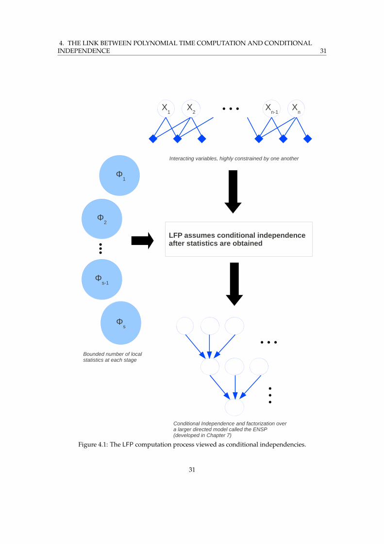
4. THE LINK BETWEEN POLYNOMIAL TIME COMPUTATION AND CONDITIONALINDEPENDENCE 31
X1
Xn
Xn-1
Interacting variables, highly constrained by one another
LFP assumes conditional independence after statistics are obtained
X2
Conditional Independence and factorization over a larger directed model called the ENSP (developed in Chapter 7)
Φs
Φ2
Φ1
Φs-1
Bounded number of local statistics at each stage
Figure 4.1: The LFP computation process viewed as conditional independencies.
31
4. THE LINK BETWEEN POLYNOMIAL TIME COMPUTATION AND CONDITIONALINDEPENDENCE 32
4.3 Conditional Independence in Complex Fixed Points
In the previous sections, we showed that the natural “factorization” of LFP into first order logic,coupled with the bounded local property of first order logic can be used to exhibit conditionalindependencies in the relation being computed.
But the argument we provided was for simple fixed points having one free variable, namely,for monadic least fixed points. How can we show that this picture is the same for complex fixedpoints? We accomplish this in stages.
1. First, we use the transitivity theorem for fixed point logic to move nested fixed points intosimultaneous fixed points without nesting.
2. Next, we use the simultaneous induction lemma for fixed point logic to encode the relationto be computed as a “section” of a single LFP relation of higher arity.
3. At this point, the picture of the preceding sections applies, except that we have to book-keep for a k-ary relation that is being computed. The property of “bounded number oflocal neighborhoods” holds at each stage, except the conditions on the neighborhoodscould be expressed in terms of k coordinates instead of just one.
Alternatively, we could work over a product structure where LFP captures the class ofpolynomial time computable queries. In other words, we have to work in a structurewhose elements are k-tuples of our original structure. In this way, a k-ary LFP over theoriginal structure would be a monadic LFP over this structure.
Steps 1 and 2 involve standard constructions in finite model theory, which we recall in Ap-pendix A. See also [EF06, §8.2]. In order to accomplish step 3, we simply have to ensure that ouroriginal structure has a relation that allows an order to be established on k-tuples. In particularthis does not pose a problem for encoding instances of k-SAT. The basic nature of informationgathering and processing in LFP does not change when the arity of the computation rises. Itmerely adds the ability to gather polynomially more information at each stage, but this infor-mation is still “bounded number of local neighborhoods at each stage.”
Remark 4.12. Note that there are elegant ways to work with the space of equivalence classesof k-tuples with equivalence under first order logic with k-variables. For instance, one canconsider a construction known as the canonical structure due originally to [DLW95] who used itto provide a model theoretic proof of the important theorem in [AV95] that P = PSPACE ifand only if LFP = PFP. Note that this is for all structures, not just for ordered structures.
The issue one faces is that there is a linear order on the canonical structure, which rendersthe Gaifman graph trivial (totally connected). See [Lib04, §11.5] for more details on canonicalstructures. The simple scheme described above suffices for our purposes.
4.4 Aggregate Properties of LFP over Ensembles
We have shown that any polynomial time computation will update its relation according toa certain Markov type property on the space of k-types of the underlying structure, after ex-tracting a statistic from the local neighborhoods of the underlying structure. Thus far, there isno probabilistic picture, or a distribution that we can analyze. We are only describing a fullydeterministic computation.
The distribution we seek will arise when we examine the aggregate behavior of LFP overensembles of structures that come from ensembles of constraint satisfaction problems (CSPs) such
32

4. THE LINK BETWEEN POLYNOMIAL TIME COMPUTATION AND CONDITIONALINDEPENDENCE 33
as random k-SAT. When we examine the properties in the aggregate of LFP running overensembles, we will find that the “bounded number of local” property of each stage of LFPcomputation manifests as conditional independencies in the distribution. This gives us thesetting where we can exploit the full machinery of graphical models of Chapter 2.
Before we examine the distributions arising from LFP acting on ensembles of structures, wewill bring in ideas from statistical physics into the proof. We begin this in the next chapter.
33

5. The 1RSB Ansatz of StatisticalPhysics
5.1 Ensembles and Phase Transitions
The study of random ensembles of various constraint satisfaction problems (CSPs) is over twodecades old, dating back at least to [CF86]. While a given CSP — say, 3-SAT— might beNP-complete, many instances of the CSP might be quite easy to solve, even using fairly simplealgorithms. Furthermore, such “easy” instances lay in certain well defined regimes of the CSP,while “harder” instances lay in clearly separated regimes. Thus, researchers were motivatedto study randomly generated ensembles of CSPs having certain parameters that would specifywhich regime the instances of the ensemble belonged to. We will see this behavior in somedetail for the specific case of the ensemble known as random k-SAT.
An instance of k-SAT is a propositional formula in conjunctive normal form
Φ = C1 ∧ C2 ∧ · · · ∧ Cm
havingm clausesCi, each of whom is a disjunction of k literals taken from n variables x1, . . . , xn.The decision problem of whether a satisfying assignment to the variables exists is NP-completefor k ≥ 3. The ensemble known as random k-SAT consists of instances of k-SAT generatedrandomly as follows. An instance is generated by drawing each of the m clauses C1, . . . , Cmuniformly from the 2k
(nk
)possible clauses having k variables. The entire ensemble of random
k-SAT having m clauses over n literals will be denoted by SATk(n,m), and a single instanceof this ensemble will be denoted by Φk(n,m). The clause density, denoted by α and defined asα := m/n is the single most important parameter that controls the geometry of the solutionspace of random k-SAT. Thus, we will mostly be interested in the case where every formulain the ensemble has clause density α. We will denote this ensemble by SATk(n, α), and anindividual formula in it by Φk(n, α).
Random CSPs such as k-SAT have attracted the attention of physicists because they modeldisordered systems such as spin glasses where the Ising spin of each particle is a binary variable(”up” or “down”) and must satisfy some constraints that are expressed in terms of the spins ofother particles. The energy of such a system can then be measured by the number of unsatisfiedclauses of a certain k-SAT instance, where the clauses of the formula model the constraintsupon the spins. The case of zero energy then corresponds to a solution to the k-SAT instance.The following formulation is due to [MZ97]. First we translate the Boolean variables xi to Isingvariables Si in the standard way, namely Si = −(−1)xi . Then we introduce new variables Cli asfollows. The variable Cli is equal to 1 if the clause Cl contains xi, it is −1 if the clause contains¬xi, and is zero if neither appears in the clause. In this way, the sum
∑ni=1 CliSi measures the
satisfiability of clause Cl. Specifically, if∑ni=1 CliSi − k > 0, the clause is satisfied by the Ising
34

5. THE 1RSB ANSATZ OF STATISTICAL PHYSICS 35
variables. The energy of the system is then measured by the Hamiltonian
H =
m∑i=1
δ(
n∑i=1
CliSi,−K).
Here δ(i, j) is the Kronecker delta. Thus, satisfaction of the k-SAT instance translates to vanish-ing of this Hamiltonian. Statistical mechanics then offers techniques such as replica symmetry,to analyze the macroscopic properties of this ensemble.
Also very interesting from the physicist’s point of view is the presence of a sharp phasetransition [CKT91, MSL92] (see also [KS94]) between satisfiable and unsatisfiable regimes ofrandom k-SAT. Namely, empirical evidence suggested that the properties of this ensembleundergoes a clearly defined transition when the clause density is varied. This transition isconjectured to be as follows. For each value of k, there exists a transition threshold αc(k) suchthat with probability approaching 1 as n→∞ (called the Thermodynamic limit by physicists),
• if α < αc(k), an instance of random k-SAT is satisfiable. Hence this region is called theSAT phase.
• If α > αc(k), an instance of random k-SAT is unsatisfiable. This region is known as theunSAT phase.
There has been intense research attention on determining the numerical value of the thresholdbetween the SAT and unSAT phases as a function of k. [Fri99] provides a sharp but non-uniformconstruction (namely, the value αc is a function of the problem size, and is conjectured to con-verge as n→∞). Functional upper bounds have been obtained using the first moment method[MA02] and improved using the second moment method [AP04] that improves as k gets larger.
5.2 The d1RSB Phase
More recently, another thread on this crossroad has originated once again from statistical physicsand is most germane to our perspective. This is the work in the progression [MZ97], [BMW00],[MZ02], and [MPZ02] that studies the evolution of the solution space of random k-SAT as theconstraint density increases towards the transition threshold. In these papers, physicists haveconjectured that there is a second threshold that divides the SAT phase into two — an “easy”SAT phase, and a “hard” SAT phase. In both phases, there is a solution with high probability,but while in the easy phase one giant connected cluster of solutions contains almost all the so-lutions, in the hard phase this giant cluster shatters into exponentially many communities thatare far apart from each other in terms of least Hamming distance between solutions that lie indistinct communities. Furthermore, these communities shrink and recede maximally far apartas the constraint density is increased towards the SAT-unSAT threshold. As this threshold iscrossed, they vanish altogether.
As the clause density is increased, a picture known as the “1RSB hypothesis” emerges thatis illustrated in Fig. 5.1, and described below.
RS For α < αd, a problem has many solutions, but they all form one giant cluster withinwhich going from one solution to another involves flipping only a finite (bounded) set ofvariables. This is the replica symmetric phase.
d1RSB At some value of α = αd which is below αc, it has been observed that the space ofsolutions splits up into “communities” of solutions such that solutions within a commu-nity are close to one another, but are far away from the solutions in any other community.
35
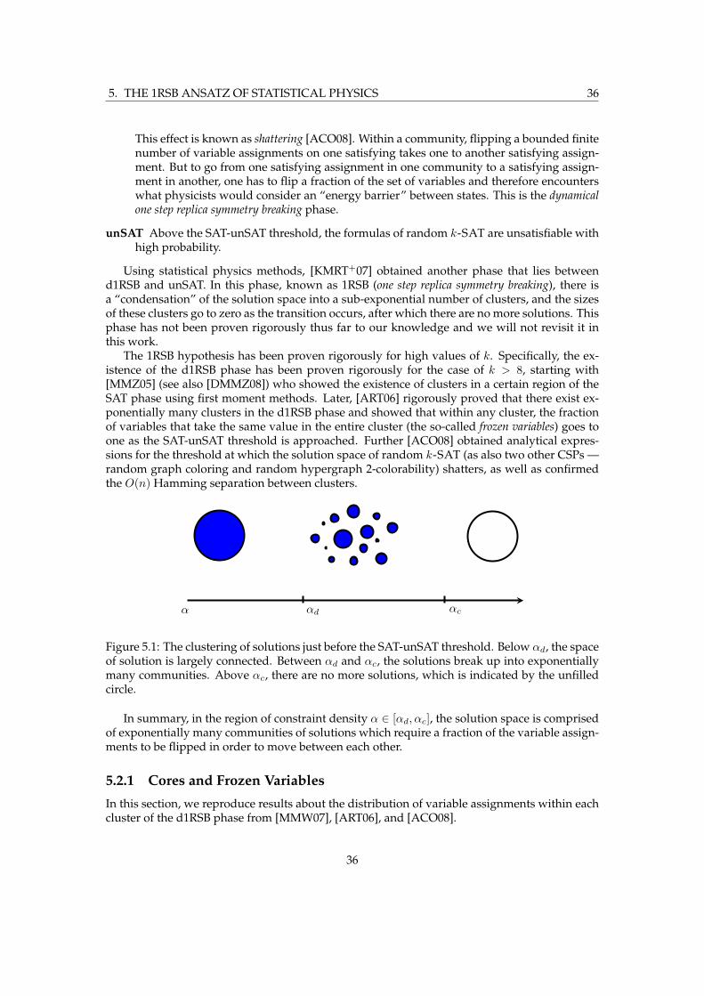
5. THE 1RSB ANSATZ OF STATISTICAL PHYSICS 36
This effect is known as shattering [ACO08]. Within a community, flipping a bounded finitenumber of variable assignments on one satisfying takes one to another satisfying assign-ment. But to go from one satisfying assignment in one community to a satisfying assign-ment in another, one has to flip a fraction of the set of variables and therefore encounterswhat physicists would consider an “energy barrier” between states. This is the dynamicalone step replica symmetry breaking phase.
unSAT Above the SAT-unSAT threshold, the formulas of random k-SAT are unsatisfiable withhigh probability.
Using statistical physics methods, [KMRT+07] obtained another phase that lies betweend1RSB and unSAT. In this phase, known as 1RSB (one step replica symmetry breaking), there isa “condensation” of the solution space into a sub-exponential number of clusters, and the sizesof these clusters go to zero as the transition occurs, after which there are no more solutions. Thisphase has not been proven rigorously thus far to our knowledge and we will not revisit it inthis work.
The 1RSB hypothesis has been proven rigorously for high values of k. Specifically, the ex-istence of the d1RSB phase has been proven rigorously for the case of k > 8, starting with[MMZ05] (see also [DMMZ08]) who showed the existence of clusters in a certain region of theSAT phase using first moment methods. Later, [ART06] rigorously proved that there exist ex-ponentially many clusters in the d1RSB phase and showed that within any cluster, the fractionof variables that take the same value in the entire cluster (the so-called frozen variables) goes toone as the SAT-unSAT threshold is approached. Further [ACO08] obtained analytical expres-sions for the threshold at which the solution space of random k-SAT (as also two other CSPs —random graph coloring and random hypergraph 2-colorability) shatters, as well as confirmedthe O(n) Hamming separation between clusters.
αd αcα
Figure 5.1: The clustering of solutions just before the SAT-unSAT threshold. Below αd, the spaceof solution is largely connected. Between αd and αc, the solutions break up into exponentiallymany communities. Above αc, there are no more solutions, which is indicated by the unfilledcircle.
In summary, in the region of constraint density α ∈ [αd, αc], the solution space is comprisedof exponentially many communities of solutions which require a fraction of the variable assign-ments to be flipped in order to move between each other.
5.2.1 Cores and Frozen Variables
In this section, we reproduce results about the distribution of variable assignments within eachcluster of the d1RSB phase from [MMW07], [ART06], and [ACO08].
36
5. THE 1RSB ANSATZ OF STATISTICAL PHYSICS 37
We first need the notion of the core of a cluster. Given any solution in a cluster, one mayobtain the core of the cluster by “peeling away” variable assignments that, loosely speakingoccur only in clauses that are satisfied by other variable assignments. This process leads to thecore of the cluster.
To get a formal definition, first we define a partial assignment of a set of variables (x1, . . . , xn)as an assignment of each variable to a value in 0, 1, ∗. The ∗ assignment is akin to a “jokerstate” which can take whichever value is most useful in order to satisfy the k-SAT formula.
Next, we say that a variable in a partial assignment is free when each clause it occurs in hasat least one other variable that satisfies the clause, or has as assignment to ∗.
Finally, to obtain the core of a cluster, we repeat the following starting with any solution inthe cluster: if a variable is free, assign it a ∗.
This process will eventually lead to a fixed point, and that is the core of the cluster. We mayeasily see that the core is not dependent upon the choice of the initial solution.
What does the core of a cluster look like? Recall that the core is itself a partial assignment,with each variable being assigned a 0, 1 or a ∗. Of obvious interest are those variables that areassigned 0 or 1. These variables are said to be frozen. Note that since the core can be arrived atstarting from any choice of an initial solution in the cluster, it follows that frozen variables takethe same value throughout the cluster. For example, if the variable xi takes value 1 in the coreof a cluster, then every solution lying in the cluster has xi assigned the value 1. The non-frozenvariables are those that are assigned the value ∗ in the core. These take both values 0 and 1 inthe cluster. Clearly the number of ∗ variables is a measure of the internal entropy (and thereforethe size) of a cluster since it is only these variables whose values vary within the cluster.
Apriori, we have no way to tell that the core will not be the all ∗ partial assignment. Namely,we do not know whether there are any frozen variables at all. However, [ART06] proved that forhigh enough values of k, with probability going to 1 in the thermodynamic limit, almost everyvariable in a core is frozen as we increase the clause density towards the SAT-unSAT threshold.
Theorem 5.1 ([ART06]). For every r ∈ [0, 12 ] there is a constant kr such that for all k ≥ kr, there exists
a clause density α(k, r) < αc such that for all α ∈ [α(k, r), αc], asymptotically almost surely
1. every cluster of solutions of Φk(n, αn) has at least (1− r)n frozen variables,
2. fewer than rn variables take the value ∗.
We end this section with a physical picture of what forms a core. If a formula Φ has acore with C clauses, then these clauses must have literals that come from a set of at most Cvariables. By bounding the probability of this event, [MMW07] obtained a lower bound on thesize of cores. The bound is linear, which means that when cores do exist ( [ART06] proved theirexistence for sufficiently high k), they must involve a fraction of all the variables in the formula.In other words, a core may be thought of as the onset of a large single interaction of degreeO(n)among the variables. As the reader may imagine after reading the previous chapters, this sortof interaction cannot be dealt with by LFP algorithms. We will need more work to make thisprecise, but informally cores are too large to pass through the bottlenecks that the stage-wisefirst order LFP algorithms create.
This may also be interpreted as follows. Algorithms based on LFP can tackle long rangeinteractions between variables, but only when they can be factored into interactions of degreepoly(log n). The exact degree is determined by the LFP algorithm — those that take more timeto complete can deal with higher degrees, but it is always poly(log n). But the appearance ofcores is equivalent to the onset of O(n) degree interactions which cannot be further factoredinto poly(log n) degree interactions. Such large interactions, caused by increasing the clausedensity sufficiently, cannot be dealt with using an LFP algorithm.
37
5. THE 1RSB ANSATZ OF STATISTICAL PHYSICS 38
We have already noted that this is because LFP algorithms factor through first order com-putations, and in a first order computation, the decision of whether an element is to enter therelation being computed is based on information collected from local neighborhoods and com-bined in a bounded fashion. This bottleneck is too small for a core to factor through. Theprecise statement of this intuitive picture will be provided in the next chapter when we buildour conditional independence hierarchies.
5.2.2 Performance of Known Algorithms
We end this chapter with a brief overview of the performance of known algorithms as a functionof the clause density, and pointers to more detailed surveys.
Beginning with [CKT91] and [MSL92], there has been an understanding that hard instancesof random k-SAT tend to occur when the constraint density α is near the transition threshold,and that this behavior was similar to phase transitions in spin glasses [KS94]. Now that wehave surveyed the known results about the geometry of the space of solutions in this region,we turn to the question of how the two are related.
It has been empirically observed that the onset of the d1RSB transition seems to coincidewith the constraint density where traditional solvers tend to exhibit exponential slowdown; see[ACO08] and [CO09]. See also [CO09] for the best current algorithm along with a comparisonof various other algorithms to it. Thus, while both regimes in SAT have solutions with highprobability, the ease of finding a solution differs quite dramatically on traditional SAT solversdue to a clustering of the solution space into numerous communities that are far apart fromeach other in terms of Hamming distance. In particular, for clause densities above O(2k/k), noalgorithms are known to produce solutions in polynomial time with probability Ω(1). Comparethis to the SAT-unSAT threshold, which is asymptotically 2k ln 2. Thus, well below the SAT-unSAT threshold, in regimes where we know solutions exist, we are currently unable to findthem in polynomial time. Our work will explain that indeed, this is fundamentally a limitationof polynomial time algorithms.
Incomplete algorithms are a class that do not always find a solution when it exists, nor dothey indicate the lack of solution except to the extent that they were unable to find one. In-complete algorithms are obviously very important for hard regimes of constraint satisfactionproblems since we do not have complete algorithms in these regimes that have economical run-ning times. More recently, a breakthrough for incomplete algorithms in this field came with[MPZ02] who used the cavity method from spin glass theory to construct an algorithm namedsurvey propagation that does very well on instances of random k-SAT with constraint densityabove the aforementioned clustering threshold, and continues to perform well very close to thethreshold αc for low values of k. Survey propagation seems to scale as n log n in this region.The algorithm uses the 1RSB hypothesis about the clustering of the solution space into nu-merous communities. The behavior of survey propagation for higher values of k is still beingresearched.
38

6. Random Graph Ensembles
We will use factor graphs as a convenient means to encode various properties of the randomk-SAT ensemble. In this section we introduce the factor graph ensembles that represent randomk-SAT. Our treatment of this section follows [MM09, Chapter 9].
Definition 6.1. The random k-factor graph ensemble, denoted by Gk(n,m), consists of graphshaving n variable nodes and m function nodes constructed as follows. A graph in the ensembleis constructed by picking, for each of the m function nodes in the graph, a k-tuple of variablesuniformly from the
(nk
)possibilities for such a k-tuple chosen from n variables.
Graphs constructed in this manner may have two function nodes connected to the same k-tuple of variables. In this ensemble, function nodes all have degree k, while the degree of thevariable nodes is a random variable with expectation km/n.
Definition 6.2. The random (k, α)-factor graph ensemble, denoted by Gk(n, α), consists of graphsconstructed as follows. For each of the
(nk
)k-tuples of variables, a function node that connects
to only these k variables is added to the graph with probability αn/(nk
).
In this ensemble, the number of function nodes is a random variable with expectation αn,and the degree of variable nodes is a random variable with expectation αk.
We will be interested in the case of the thermodynamic limit of n,m → ∞ with the ratioα := m/n being held constant. In this case, both the ensembles converge in the propertiesthat are important to us, and both can be seen as the underlying factor graph ensembles to ourrandom k-SAT ensemble SATk(n, α) (see Chapter 5 for definitions and our notation for randomk-SAT ensembles).
With the definitions in place, we are ready to describe two properties of random graphensembles that are pertinent to our problem.
6.1 Properties of Factor Graph Ensembles
The first property provides us with intuition on why algorithms find it so hard to put togetherlocal information to form a global perspective in CSPs.
6.1.1 Locally Tree-Like Property
We have seen in Chapter 4 that the propagation of influence of variables during a LFP compu-tation is stagewise-local. This is really the fundamental limitation of LFP that we seek to exploit.In order to understand why this is a limitation, we need to examine what local neighborhoodsof the factor graphs underlying NP-complete problems like k-SAT look like in hard phasessuch as d1RSB. In such phases, there are many extensive (meaning O(n)) correlations betweenvariables that arise due to loops of sizes O(log n) and above.
39

6. RANDOM GRAPH ENSEMBLES 40
However, remarkably, such graphs are locally trivial. By that we mean that there are no cyclesin a O(1) sized neighborhood of any vertex as the size of the graph goes to infinity [MM09,§9.5]. One may demonstrate this for the Erdos-Renyi random graph as follows. Here, there aren vertices, and there is an edge between any two with probability c/n where c is a constantthat parametrizes the density of the graph. Edges are “drawn” uniformly and independentlyof each other. Consider the probability of a certain graph (V,E) occurring as a subgraph of theErdos-Renyi graph. Such a graph can occur in
(n|V |)
positions. At each position, the probabilityof the graph structure occurring is
p|E|(1− p)|V |2 −|E|.
Applying Stirling’s approximations, we see that such a graph occurs asymptoticallyO(|V |−|E|)times. If the graph is connected, |V | ≤ |E| − 1 with equality only for trees. Thus, in the limit ofn→∞, finite connected graphs have vanishing probability of occurring in finite neighborhoodsof any element.
In short, if only local neighborhoods are examined, the two ensembles Gk(n,m) and Tk(n,m)are indistinguishable from each other.
Theorem 6.3. LetG be a randomly chosen graph in the ensemble Gk(n,m), and i be a uniformly chosennode in G. Then the r-neighborhood of i in G converges in distribution to Tk(n,m) as n→∞.
Let us see what this means in terms of the information such graphs divulge locally. Thesimplest local property is degrees of elements. These are, of course, available through localinspection. The next would be small connected subgraphs (triangles, for instance). But eventhis next step is not available. In other words, such random graphs do not provide any of theirglobal properties through local inspection at each element.
Let us think about what this implies. We know from the onset of cores and frozen variablesin the 1dRSB phase of k-SAT that there are strong correlations between blocks of variables ofsizeO(n) in that phase. However, these loops are invisible when we inspect local neighborhoodsof a fixed finite size, as the problem size grows.
6.1.2 Degree Profiles in Random Graphs
The degree of a variable node in the ensemble Gk(n,m) is a random variable. We wish to under-stand the distribution of this random variable. The expected value of the fraction of variablesin Gk(n,m) having degree d is the same as the expected value that a single variable node hasdegree d, both being equal to
P (deg vi = d) =
(m
d
)pk(1− p)m−d where p =
k
d.
In the large graph limit we get
limn→∞
P (deg vi = d) = e−kα(kα)d
n !.
In other words, the degree is asymptotically a Poisson random variable.A corollary is that the maximum degree of a variable node is almost surely less thanO(log n)
in the large graph case.
40
6. RANDOM GRAPH ENSEMBLES 41
Lemma 6.4. The maximum variable node degree in Gk(n,m) is asymptotically almost surely O(log n).In particular, it asymptotically almost surely satisfies the following
dmax
kαe=
z
log(z/ log z)
[1 + Θ
(log log z
(log z)2
)]. (6.1)
where z = (log n)/kαe.
Proof. See [MM09, p. 184] for a discussion of this upper bound, as well as a lower bound.
41
7. Separation of Complexity Classes
We have built a framework that connects ideas from graphical models, logic, statistical mechan-ics, and random graphs. We are now ready to begin our final constructions that will yield theseparation of complexity classes.
7.1 Measuring Conditional Independence
The central concern of this work has been to understand what are the irreducible interactionsbetween the variables in a system — namely, those that cannot be expressed in terms of inter-actions between smaller sets of variables with conditional independencies between them. Suchirreducible interactions can be 2-interactions (between pairs), 3-interactions (between triples),and so on, up to n-interactions between all n variables simultaneously.
A joint distribution encodes the interaction of a system of n variables. What would happenif all the direct interactions between variables in the system were all of less than a certain finiterange k, with k < n? In such a case, the “jointness” of the covariates really would lie at alower “level” than n. We would like to measure the “level” of conditional independence ina system of interacting variables by inspecting their joint distribution. At level zero of this“hierarchy”, the covariates should be independent of each other. At level n, they are coupledtogether n at a time, without the possibility of being decoupled. In this way, we can makestatements about how deeply entrenched the conditional independence between the covariatesis, or dually, about how large the set of direct interactions between variables is.
This picture is captured by the number of independent parameters required to parametrizethe distribution. When the largest irreducible interactions are k-interactions, the distributioncan be parametrized with n2k independent parameters. Thus, in families of distributions wherethe irreducible interactions are of fixed size, the independent parameter space grows polynomi-ally with n, whereas in a general distribution without any conditional independencies, it growsexponentially with n. The case of LFP lies in between — the interactions are not of fixed size,but they grow relatively slowly.
There are some technical issues with constructing such a hierarchy to measure conditionalindependence. The first issue would be how to measure the level of a distribution in this hier-archy. If, for instance, the distribution has a directed P-map, then we could measure the sizeof the largest clique that appears in its moralized graph. However, as noted in Sec. 2.5, notall distributions have such maps. We may, of course, upper and lower bound the level usingminimal I-maps and maximal D-maps for the distribution. In the case of ordered graphs, weshould note that there may be different minimal I-maps for the same distribution for differentorderings of the variables. See [KF09, p. 80] for an example.
The insight that allows us to resolve the issue is as follows. If we could somehow embed thedistribution of solutions generated by LFP into a larger distribution, such that
1. the larger distribution factorized recursively according to some directed graphical model,
42

7. SEPARATION OF COMPLEXITY CLASSES 43
and
2. the larger distribution had only polynomially many more variates than the original one,
then we would have obtained a parametrization of our distribution that would reflect the fac-torization of the larger distribution, and would cost us only polynomially more, which does notaffect us.
By pursuing the above course, we aim to demonstrate that distributions of solutions gener-ated by LFP lie at a lower level of conditional independence than distributions that occur in thed1RSB phase of random k-SAT. Consequently, they have more economical parametrizationsthan the space of solutions in the 1dRSB phase does.
We will return to the task of constructing such an embedding in Sec. 7.3. First we describehow we use LFP to create a distribution of solutions.
7.2 Generating Distributions from LFP
7.2.1 Encoding k-SAT into Structures
In order to use the framework from Chapters 3 and 4, we will encode k-SAT formulae as struc-tures over a fixed vocabulary.
Our vocabularies are relational, and so we need only specify the set of relations, and the setof constants. We will use three relations.
1. The first relation RC will encode the clauses that a SAT formula comprises. Since we arestudying ensembles of random k-SAT, this relation will have arity k.
2. We need a relation in order to make FO(LFP) capture polynomial time queries on the classof k-SAT structures. We will not introduce a linear ordering since that would make theGaifman graph a clique. Rather we will include a relation such that FO(LFP) can captureall the polynomial time queries on the structure. This will be a binary relation RE .
3. Lastly, we need a relation RP to hold “partial assignments” to the SAT formulae. We willdescribe these in the Sec. 7.2.3.
4. We do not require constants.
This describes our vocabularyσ = RC , RE , RP .
Next, we come to the universe. A SAT formula is defined over n variables, but they can comeeither in positive or negative form. Thus, our universe will have 2n elements corresponding tothe variables x1, . . . , xn,¬x1, . . . ,¬xn. In order to avoid new notation, we will simply use thesame notation to indicate the corresponding element in the universe. We denote by lower casexi the literals of the formula, while the corresponding upper case Xi denotes the correspondingvariable in a model.
Finally, we need to interpret our relations in our universe. We dispense with the superscriptssince the underlying structure is clear. The relationRC will consist of k-tuples from the universeinterpreted as clauses consisting of disjunctions between the variables in the tuple. The relationRE will be interpreted as an “edge” between successive variables. The relation RP will be apartial assignment of values to the underlying variables.
Now we encode our k-SAT formulae into σ-structures in the natural way. For example,for k = 3, the clause x1 ∨ ¬x2 ∨ ¬x3 in the SAT formula will be encoded by inserting the
43

7. SEPARATION OF COMPLEXITY CLASSES 44
tuple (x1,¬x2,¬x3) in the relation RC . Similarly, the pairs (xi, xi+1) and (¬xi,¬xi+1), both for1 ≤ i < n, as well as the pair (xn,¬x1) will be in the relation RE . This chains together theelements of the structure.
The reason for the relation RE that creates the chain is that on such structures, polynomialtime queries are captured by FO(LFP) [EF06, §11.2]. This is a technicality. Recall that an orderon the structure enables the LFP computation (or the Turing machine the runs this computation)to represent tuples in a lexicographical ordering. In our problem k-SAT, it plays no further role.Specifically, the assignments to the variables that are computed by the LFP have nothing to dowith their order. They depend only on the relation RC which encodes the clauses and the rela-tion RP that holds the initial partial assignment that we are going to ask the LFP to extend. Inother words, each stage of the LFP is order-invariant. It is known that the class of order invariantqueries is also Gaifman local [GS00]. However to allow LFP to capture polynomial time on theclass of encodings, we need to give the LFP something it can use to create an ordering. We couldencode our structures with a linear order, but that would make the Gaifman graph fully con-nected. What we want is something weaker, that still suffices. Thus, we encode our structuresas successor-type structures through the relation RE . This seems most natural, since it impartson the structure an ordering based on that of the variables. Note also that SAT problems mayalso be represented as matrices (rows for clauses, columns for variables that appear in them),which have a well defined notion of order on them.
Ensembles of k-SAT Let us now create ensembles of σ-structures using the encoding de-scribed above. We will start with the ensemble SATk(n, α) and encode each k-SAT instance asa σ-structure. The resulting ensemble will be denoted by Sk(n, α). The encoding of the problemΦk(n, α) as a σ-structure will be denoted by Pk(n, α).
7.2.2 The LFP Neighborhood System
In this section, we wish to describe the neighborhood system that underlies the monadic LFPcomputations on structures of Sk(n, α). We begin with the factor graph, and build the neigh-borhood system through the Gaifman graph.
Let us recall the factor graph ensemble Gk(n,m). Each graph in this ensemble encodesan instance of random k-SAT. We encode the k-SAT instance as a structure as described inthe previous section. Next, we build the Gaifman graph of each such structure. The set ofvertices of the Gaifman graph are simply the set of variable nodes in the factor graph and theirnegations since we are using both variables and their negations for convenience (this is simplyan implementation detail). For instance, the Gaifman graph for the factor graph of Fig 2.2 willhave 12 vertices. Two vertices are joined by an edge in the Gaifman graph either when the twocorresponding variable nodes were joined to a single function node (i.e., appeared in a singleclause) of the factor graph or if they are adjacent to each other in the chain that relation RE hascreated on the structure.
On this Gaifman graph, the simple monadic LFP computation induces a neighborhood sys-tem described as follows. The sites of the neighborhood system are the variable nodes. Theneighborhood Ns of a site s is the set of all nodes that lie in the r-neighborhood of a site, wherer is the locality rank of the first order formula ϕ whose fixed point is being constructed by theLFP computation.
Finally, we make the neighborhood system into a graph in the standard way. Namely, thevertices of the graph will be the set of sites. Each site s will be connected by an edge to everyother site in Ns. This graph will be called the interaction graph of the LFP computation. Theensemble of such graphs, parametrized by the clause density α, will be denoted by Ik(n, α).
44
7. SEPARATION OF COMPLEXITY CLASSES 45
Note that this interaction graph has many more edges in general than the Gaifman graph.In particular, every node that was within the locality rank neighborhood of the Gaifman graphis now connected to it by a single edge. The resulting graph is, therefore, far more dense thanthe Gaifman graph.
What is the size of cliques in this interaction graph? This is not the same as the size of cliquesin the factor graph, or the Gaifman graph, because the density of the graph is higher. The sizeof the largest clique is a random variable. What we want is an asymptotic almost sure (by thiswe mean with probability tending to 1 in the thermodynamic limit) upper bound on the size ofthe cliques in the distribution of the ensemble Ik(n, α).
Note: From here on, all the statements we make about ensembles should be understood to hold asymp-totically almost surely in the respective random ensembles. By that we mean that they hold with proba-bility 1 as n→∞.
Lemma 7.1. The size of cliques that appear in graphs of the ensemble Ik(n, α) are upper bounded bypoly(log n) asymptotically almost surely.
Proof. Let dmax be as in (6.1), and r be the locality rank of ϕ. The maximum degree of a nodein the Gaifman graph is asymptotically almost surely upper bounded by dmax = O(log n). Thelocality rank is a fixed number (roughly equal to 3d where d is the quantifier depth of the firstorder formula that is being iterated). The node under consideration could have at most dmax
others adjacent to it, and the same for those, and so on. This gives us a coarse drmax upper boundon the size of cliques.
Remark 7.2. While this bound is coarse, there is not much point trying to tighten it because anyconstant power factor (r in the case above) can always be introduced by computing a r-ary LFPrelation. This bound will be sufficient for us.
Remark 7.3. High degree nodes in the Gaifman graph become significant features in the interac-tion graph since they connect a large number of other nodes to each other, and therefore allowthe LFP computation to access a lot of information through a neighborhood system of givenradius. It is these high degree nodes that reduce factorization of the joint distribution since theyrepresent direct interaction of a large number of variables with each other. Note that althoughthe radii of neighborhoods areO(1), the number of nodes in them is notO(1) due to the Poissondistribution of the variable node degrees, and the existence of high degree nodes.
Remark 7.4. The relation being constructed is monadic, and so it does not introduce new edgesinto the Gaifman graph at each stage of the LFP computation. When we compute a k-ary LFP,we can encode it into a monadic LFP over a polynomially (nk) larger product space, as is donein the canonical structure, for instance, but with the linear order replaced by a weaker succes-sor type relation. Therefore, we can always chose to deal with monadic LFP. This is really arestatement of the transitivity principle for inductive definitions that says that if one can writean inductive definition in terms of other inductively defined relations over a structure, then onecan write it directly in terms of the original relations that existed in the structure [Mos74, p. 16].
7.2.3 Generating Distributions
The standard scenario in finite model theory is to ask a query about a structure and obtain aYes/No answer. For example, given a graph structure, we may ask the query “Is the graphconnected?” and get an answer.
But what we want are distributions of solutions that are computed by a purported LFP al-gorithm for k-SAT. This is not generally the case in finite model theory. Intuitively, we wantto generate solutions lying in exponentially many clusters of the solution space of SAT in the
45
7. SEPARATION OF COMPLEXITY CLASSES 46
d1RSB phase. How do we do this? To generate these distributions, we will start with partialassignments to the set of variables in the formula, and ask the question whether such a partialassignment can be extended to a satisfying assignment. Since the answer to such a question canbe verified in polynomial time, such a query must be expressible in FO(LFP) itself on our en-coding of k-SAT into structures if P = NP. In fact, through the self-reducibility of SAT, we cansee that the resulting assignment will itself be expressible as a LFP computable global relation.
Since we want to generate exponentially many such solutions, we will have to partially as-sign O(n) (a small fraction) of the variables, and ask the LFP to extend this assignment, when-ever possible, to a satisfying assignment to all variables. Thus, we now see what the relationRP in our vocabulary stands for. It holds the partial assignment to the variables. For example,suppose we want to ask whether the partial assignment x1 = 1, x2 = 0, x3 = 1 can be extendedto a satisfying assignment to the SAT formula, we would store this partial assignment in thetuple (x1,¬x2, x3) in the relation RP in our structure.
The output satisfying assignment will be computed as a unary relation which holds all theliterals that are assigned the value 1. This means that xi is in the relation if xi has been assignedthe value 1 by the LFP, and otherwise¬xi is in the relation meaning that xi has been assigned thevalue 0 by the LFP computation. This is the simplest case where the FO(LFP) formula is simplemonadic. For more complex formulas, the output will be some section of a relation of higherarity (please see Appendix A for details), and we will view it as monadic over a polynomiallylarger structure.
Now we “initialize” our structure with different partial assignments and ask the LFP tocompute complete assignments when they exist. If the partial assignment cannot be extended,we simply abort that particular attempt and carry on with other partial assignments until wegenerate enough solutions. By “enough” we mean rising exponentially with the underlyingproblem size. In this way we get a distribution of solutions that is exponentially numerous, andwe now analyze it and compare it to the one that arises in the d1RSB phase of random k-SAT.
7.3 Disentangling the Interactions: The ENSP Model
Now that we have a distribution of solutions computed by LFP, we would like to examineits conditional independence characteristics. Does it factor through any particular graphicalmodel, for instance?
In Chapter 2, we considered various graphical models and their conditional independencecharacteristics. Once again, our situation is not exactly like any of these models. We will haveto build our own, based on the principles we have learnt. Let us first note two issues.
The first issue is that graphical models considered in literature are mostly static. By this wemean that
1. they are of fixed size, over a fixed set of variables, and
2. the relations between the variables encoded in the models are fixed.
In short, they model fixed interactions between a fixed set of variables. Since we wish toapply them to the setting of complexity theory, we are interested in families of such models,with a focus on how their structure changes with the problem size.
The second issue that faces us now is as follows. Even within a certain size n, we do not havea fixed graph on n vertices that will model all our interactions. The way a LFP computationproceeds through the structure will, in general, vary with the initial partial assignment. Wewould expect a different “trajectory” of the LFP computation for different clusters in the 1dRSBphase. So, if one initial partial assignment landed us in cluster X, and another in cluster Y, the
46

7. SEPARATION OF COMPLEXITY CLASSES 47
way the LFP would go about assigning values to the unassigned variables would be, in general,quite different. Even within a cluster, the trajectories of two different initial partial assignmentswill not be the same, although we would expect them to be similar. How do we deal with thissituation?
In order to model this dynamic behavior, let us build some intuition first.
1. We know that there is a “directed-ness” to LFP in that elements that are assigned values ata certain stage of the computation then go on to influence other elements who are as yetunassigned. Thus, there is a directed flow of influence as the LFP computation progresses.This is, for example, different from a Markov random field distribution which has no suchdirection.
2. There are two types of flows of information in a LFP computation. Consider simplemonadic LFP. In one type of flow, neighborhoods across the structure influence the valuean unassigned node will take. In the other type of flow, once an element is assigned avalue, it changes the neighborhoods (or more precisely the local types of various otherelements) in its vicinity. Note that while the first type of flow happens during a stage ofthe LFP, the second type is implicit. Namely, there is no separate stage of the LFP whereit happens. It implicitly happens once any element enters the relation being computed.
3. Because the flow of information is as described above, we will not be able to express itusing a simple DAG on either the set of vertices, or the set of neighborhoods. Thus, wehave to consider building a graphical model on certain larger product spaces.
4. The stage-wise nature of LFP is central to our analysis, and the various stages cannot bebundled into one without losing crucial information. Thus, we do need a model whichcaptures each stage separately.
5. In order to exploit the factorization properties of directed graphical models, and the result-ing parametrization by potentials, we would like to avoid any closed directed paths.
Let us now incorporate this intuition into a model, which we will call a Element-Neighborhood-Stage Product Model, or ENSP model for short. This model appears to be of independent inter-est. We now describe the ENSP model for a simple monadic least fixed point computation. Themodel is illustrated in Fig. 7.1. It has two types of vertices.
Element Vertices These vertices, which encode the variables of the k-SAT instance, are rep-resented by the smaller circles in Fig. 7.1. They therefore correspond to elements in thestructure (recall that elements of the structure represent the literals in the k-SAT formula).However, each variable in our original system X1, . . . , Xn is represented by a different vertex ateach stage of the computation. Thus, each variable in the original system gives rise to |ϕA|vertices in the ENSP model. Also recall that there are 2n elements in the k-SAT structure,where n is the number of variables in the SAT formula. However, in Fig 7.1, we have onlyshown one vertex per variable, and allowed it to be colored two colors - green indicatingthe variable has been assigned a value of +1, and red indicating the variable has beenassigned the value −1. Since the underlying formula ϕ that is being iterated is positive,elements do not change their color once they have been assigned.
Neighborhood Vertices These vertices, denoted by the larger circles with blue shading in Fig. 7.1,represent the r-neighborhoods of the elements in the structure. Just like variables, eachneighborhood is also represented by a different vertex at each stage of the LFP com-putation. Each of their possible values are the possible isomorphism types of the r-neighborhoods, namely, the local r-types of the corresponding element. These vertices
47
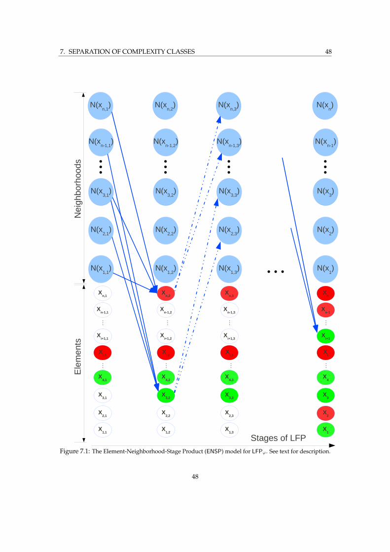
7. SEPARATION OF COMPLEXITY CLASSES 48
N(x1,1
)
X1,1
N(x2,1
)
N(x3,1
)
N(xn-1,1
)
N(xn,1
)
N(x1,2
)
N(x2,2
)
N(x3,2
)
N(xn-1,2
)
N(xn,2
)
N(x1,3
)
N(x2,3
)
N(x3,3
)
N(xn-1,3
)
N(xn,3
)
N(x1)
N(x2)
N(x3)
N(xn-1
)
N(xn)
⋮
X2,1
X3,1
X4,1
Xi,1
Xi+1,1
Xn-1,1
Xn,1
⋮
⋮
X1,2
X2,2
X3,2
X4,2
Xi,2
Xi+1,2
Xn-1,2
Xn,2
X1,3
X2,3
X3,3
X4,3
Xi,3
Xi+1,3
Xn-1,3
Xn,3
X1
X2
X3
X4
Xi
Xi+1
Xn-1
Xn
⋮⋮
⋮ ⋮ ⋮
Stages of LFP
Ele
men
tsN
eigh
borh
oods
Figure 7.1: The Element-Neighborhood-Stage Product (ENSP) model for LFPϕ. See text for description.
48
7. SEPARATION OF COMPLEXITY CLASSES 49
may be thought of as vectors of size poly(log n) corresponding to the cliques that occur inthe neighborhood system we described in Sec. 7.2.2, or one may think of them as a singlevariable taking the value of the various local r-types.
Now we describe the stages of the ENSP. There are 2|ϕA| stages, starting from the leftmostand terminating at the rightmost. Each stage of the LFP computation is represented by twostages in the ENSP. Initially, at the start of the LFP computation, we are in the left-most stage.Here, notice that some variable vertices are colored green, and some red. In the figure, X4,1 isgreen, and Xi,1 is red. This indicates that the initial partial assignment that we provided theLFP had variable X4 assigned +1 and variable Xi assigned −1. In this way, a small fractionO(n) of the variables are assigned values. The LFP is asked to extend this partial assignment toa complete satisfying assignment on all variables (if it exists, and abort if not).
Let us now look at the transition to the second stage of the ENSP. At this stage, based onthe conditions expressed by the formula ϕ in terms of their own local neighborhoods, and theexistence of a bounded number of other local neighborhoods in the structure, some elementsenter the relation. This means they get assigned +1 or −1. In the figure, the variable X3,2
takes the color green based on information gathered from its own neighborhood N(X3,1) andtwo other neighborhoods N(X2,1) and N(Xn−1,1). This indicates that at the first stage, theLFP assigned the value +1 to the variable X3. Similarly, it assigns the value −1 to variableXn (remember that the first two stages in the ENSP correspond to the first stage of the LFPcomputation). The vertices that do not change state simply transmit their existing state to thecorresponding vertices in the next stage by a horizontal arrow, which we do not show in thefigure in order to avoid clutter.
Once some variables have been assigned values in the first stage, their neighborhoods, andthe neighborhoods in their vicinity (meaning, the neighborhoods of other elements that are intheir vicinity) change. This is indicated by the dotted arrows between the second and thirdstages of the ENSP. Note that this happens implicitly during LFP computation. That is why wehave represented each stage of the actual LFP computation by two stages in the ENSP. The firststage is the explicit stage, where variables get assigned values. The second stage is the implicitstage, where variables “update their neighborhoods” and those neighborhoods in their vicinity.For example, once X3 has been assigned the value +1, it updates its neighborhood and also theneighborhood of variable X2 which lies in its vicinity (in this example). In this way, influencepropagates through the structure during a LFP computation. There are two stages of the ENSPfor each stage of the LFP. Thus, there are 2|ϕA| stages of the ENSP in all.
By the end of the computation, all variables have been assigned values, and we have asatisfying assignment. The variables at the last stage Xi,|ϕA| are just the original Xi. Thus, werecover our original variables (X1, . . . , Xn) by simply looking only at the last (rightmost in thefigure) level of the ENSP.
By introducing extra variables to represent each stage of each variable and each neighbor-hood in the SAT formula, we have accomplished our original aim. We have embedded ouroriginal set of variates into a polynomially larger product space, and obtained a directed graph-ical model on this larger space. This product space has a nice factorization due to the directedgraph structure. This is what we will exploit.
Remark 7.5. The explicit stages of the ENSP also perform the task of propagating the local con-straints placed by the various factors in the underlying factor graph outward into the largergraphical model. For example, in our case of the factors encoding clauses of a k-SAT formula,the local constraint placed by a clause is that the global assignment must evade exactly onerestriction to a specified set of k coordinates. For example, in the case of k = 3 the clausex1 ∨ x2 ∨ ¬x3 permits all global assignments except those whose first three coordinates are
49

7. SEPARATION OF COMPLEXITY CLASSES 50
(−1,−1,+1). In contrast, if the factor were a XORSAT clause, the local restrictions are all in theform of linear spaces, and so the global solution is an intersection of such spaces. k-SAT asks aquestion about whether certain spaces of the form
ω : (ωi1 , . . . , ωik) 6= (ν1, . . . , νk)
have non-empty intersections, where 1 ≤ i1 < i2 < · · · < ik ≤ n and the prohibited νi are ±1.Note that these are O(1) local constraints per factor. In contrast, XORSAT asks the questionabout whether certain linear spaces have a non-empty intersection. Linearity is a global con-straint. Of course, all messages are coded into the formula ϕ. Thus, the end result of multipleruns of the LFP will be a space of solutions conditioned upon the requirements. So, for instance,if we were to try to solve XORSAT formulae, we would obtain a space that would be linear.
Thus, we have a directed graph with 2n + n = 3n vertices at each stage, and 2|ϕA| stages.Since the LFP completes its computation in under a fixed polynomial number of steps, thismeans that we have managed to represent the LFP computation on a structure as a directedmodel using a polynomial overhead in the number of parameters of our representation space.In other words, by embedding the covariates into a polynomially larger space, we have beenable to put a common structure on various computations done by LFP on them. In the ENSPmodel, the covariates are recovered by restricting to the first n vertices in the bottom row, butnow we have a graphical model that can represent the underlying computation done in order toget to that final state. Note that without embedding the covariates into a larger space, we wouldnot be able to place the various computations done by LFP into a single graphical model. Theinsight that we can afford to incur a polynomial cost in order to obtain a common graphicalmodel on a larger product space was key to this section.
7.4 Parametrization of the ENSP
Our goal is to demonstrate the following.
If LFP were able to compute solutions to the d1RSB phase of random k-SAT, then the dis-tribution of the entire space of solutions would have a substantially simpler parametrizationthan we know it does.
In order to accomplish this, we need to measure the growth in the dimension of independentparameters it requires to parametrize the distribution of solutions that we have just computedusing LFP.
In order to do this, we have embedded our variates into a polynomially larger space thathas factorization according to a directed model — the ENSP. We have seen that the cliques inthe ENSP are of size poly(log n). By employing the version of Hammersley-Clifford for directedmodels, Theorem 2.13, we also know that we can parameterize the distribution by specifying asystem of potentials over its cliques, automatically ensuring conditional independence.
The directed nature of the ENSP also means that we can factor the resulting distribution intoconditional probability distributions (CPDs) at each vertex of the model of the formP (x | pa(x)),and then normalize each CPD. Once again, each CPD will have scope only poly(log n). Fromour perspective, the major benefit of directed graphical models is that we can do this always,without any added positivity constraints. Recall that positivity is required in order to apply theHammersley-Clifford theorem to obtain factorizations for undirected models.
How do we compute the CPDs or potentials? We assign various initial partial assignmentsto the variables as described in Sec. 7.2.3 and let the LFP computations run. We only consider
50
7. SEPARATION OF COMPLEXITY CLASSES 51
successful computations, namely those where the LFP was able to extend the partial assignmentto a full satisfying assignment to the underlying k-SAT formula. We represent each stage ofthe LFP computation on the corresponding two stages of the ENSP and thus obtain one fullinstantiation of the representation space. We do this exponentially numerous times, and buildup our local CPDs by simply recording local statistics over all these runs. This gives us thefactorization (over the expanded representation space) of our distribution, assuming that P =NP.
The ENSP for different runs of the LFP will, in general, be different. This is because theflow of influences through the stages of the ENSP will, in general, depend on the initial partialassignment. What is important is that each such model will have some properties — such aslargest clique size, which determines the order of the number of parameters — in common. Letus inspect these properties that determine the parametrization of the ENSP model.
1. There are polynomially many more vertices in the ENSP model than elements in the un-derlying structure.
2. Lemma 7.1 gives us a poly(log n) upper bound on the size of the neighborhoods. Thenumber of local r-types whose value each neighborhood vertex can take is 2poly(logn).
3. By Theorem 4.8 there is a fixed constant s such that there must exist s neighborhoods inthe structure satisfying certain local conditions for the formula to hold. Remember, weare presently analyzing a single stage of the LFP. This again gives us poly(n) (O(ns) inthis case) different possibilities for each explicit stage of the ENSP. The same can alsobe arrived at by utilizing the normal form of Theorem 4.9. By the previous point, eachof these possibilities can be parameterized by 2poly(logn) parameters, giving us a total of2poly(logn) parameters required.
4. At each implicit stage of the ENSP, we have to update the types of the neighborhoods thatwere affected by the induction of elements at the previous explicit stage. There are only nneighborhoods, and each has poly(log n) elements at most.
The ENSP is an interaction model where direct interactions are of size poly(log n), and are chainedtogether through conditional independencies.
Proposition 7.6. A distribution that factorizes according to the ENSP can be parameterized with2poly(logn) independent parameters. The scope of the factors in the parametrization grows as poly(log n).
This also underscores the principle that the description of the parameter space is simplerbecause it only involves interactions between l variates at a time directly, and then chains thesetogether through conditional independencies. In the case of the LFP neighborhood system, thesize of the largest cliques are poly(log n) for each single run of the LFP. This will not change ifwe were computing using complex fixed points since the space of k-types is only polynomiallylarger than the underlying structure.
The crucial property of the distribution of the ENSP is that it admits a recursive factorization.This is what drastically reduces the parameter space required to specify the distribution. Italso allows us to parametrize the ENSP by simply specifying potentials on its maximal cliques,which are of size poly(log n).
While the entire distribution obtained by LFP may not factor according to any one ENSP,it is a mixture of distributions each of whom factorizes as per some ENSP. Next, we analyzethe features of such a mixture when exponentially many instantiations of it are provided. Asthe reader may intuit, when such a mixture is asked to provide exponentially many samples,these will show features of scope poly(log n). This is simply a statement about the paucity ofindependent parameters in the component distributions in the mixture.
51
7. SEPARATION OF COMPLEXITY CLASSES 52
7.5 Separation
The property of the ENSP that allows us to analyze the behavior of mixtures is that it is spec-ified by local Gibbs potentials on its cliques. In other words, a variable interacts with the restof the model only through the cliques that it is part of. These cliques are parametrized by po-tentials. We may think of the cliques as the building blocks of each ENSP. The cliques are alsoupper bounded in size by poly(log n). Furthermore, a vertex may be in at most O(log n) suchcliques. Therefore, a vertex displays collective behavior only of range poly(log n). Thus, themixture comprises distributions that can be parametrized by a subspace of Rpoly(logn), in con-trast to requiring the larger space RO(n). This means that when exponentially many solutionsare generated, the features in the mixture will be of size poly(log n), not of size O(n).
This explains why polynomial time algorithms fail when interactions between variable areO(n) at a time, without the possibility of factoring into smaller pieces through conditional inde-pendencies. This also puts on rigorous ground the empirical observation that even NP-completeproblems are easy in large regimes, and become hard only when the densities of constraints in-crease above a certain threshold. This threshold is precisely the value where O(n) interactionsfirst appear in almost all randomly constructed instances.
In case of random k-SAT in the d1RSB phase, these irreducible O(n) interactions manifestthrough the appearance of cores which comprise clauses whose variables are coupled so tightlythat one has to assign them “simultaneously.” Cores arise when a set of C = O(n) clauses haveall their variables also lying in a set of size C. Once clause density is sufficiently high, cores can-not be assigned poly(log n) at a time, and successive such assignments chained together throughconditional independencies. Since cores do not factor through conditional independencies, thismakes it impossible for polynomial time algorithms to assign their variables correctly. Intu-itively, variables in a core are so tightly coupled together that they can only vary jointly, withoutany conditional independencies between subsets. In other words, they represent irreducible in-teractions of size O(n) which may not be factored any further. In such cases, parametrizationover cliques of size only poly(log n) is insufficient to specify the joint distribution.
However, we have shown that in the ENSP model, the size of the largest such irreducibleinteractions are poly(log n), not O(n). Furthermore, since the model is directed, it guarantees usconditional independencies at the level of its largest interactions. More precisely, it guaranteesus that there will exist conditional independencies in sets of size larger than the largest cliquesin its moral graph, which are O(poly(log n)). In other words, there will be independent vari-ation within cores when conditioned upon values of intermediate variables that also lie withinthe core, should the core factorize as per the ENSP. This is illustrated in Fig. 7.2. This is contra-dictory to the known behaviour of cores for sufficiently high values of k and clause density inthe d1RSB phase. In other words, while the space of solutions generated by LFP has features ofsize poly(log n), the features present in cores in the d1RSB phase have size O(n).
The framework we have constructed allows us to analyze the set of polynomial time algo-rithms simultaneously, since they can all be captured by some LFP, instead of dealing witheach individual algorithm separately. It makes precise the notion that polynomial time algo-rithms can take into account only interactions between variables that grow as poly(log n),not as O(n).
At this point, we are ready to state our main theorem.
Theorem 7.7. P 6= NP.
Proof. Consider the solution space of k-SAT in the d1RSB phase for k > 8 as recalled in Section.5.2.1.We know that for high enough values of the clause density α, we have O(n) frozen variables
52

7. SEPARATION OF COMPLEXITY CLASSES 53
poly(log n) poly(log n)
Independent given Intermediate values
Independent given Intermediate values
Figure 7.2: The factorization within a core due to potentials of size poly(log n).
in almost all of the exponentially many clusters. Let us consider the situation where these clus-ters were generated by a purported LFP algorithm for k-SAT. However, when exponentiallymany solutions have been generated from distributions having the parametrization of the ENSPmodel, we will see the effect of conditional independencies beyond range poly(log n). Let αβγbe a representation of the variables in cliques α, β and γ, then given a value of β, we will seeindependent variation over all their possible conditional values in the variables of α and γ. Ifeach set of such variables has scope at most poly(log n), then this means that once more thancpoly(logn), c > 1 many distinct solutions are generated, we have non-trivial conditional distri-butions conditioned upon values of β variables (this factor accounts for the possible orderingswithin the poly(logn) variables as well). At this point, the conditional independence ensurethat we will see cross terms of the form
α1βγ1 α2βγ2 α1βγ2 α2βγ1.
Note that since O(n) variables have to be changed when jumping from one cluster to another,we may even chose our poly(log n) blocks to be in overlaps of these variables. This wouldmean that with a poly(log n) change in frozen variables of one cluster, we would get a solutionin another cluster. But we know that in the highly constrained phases of d1RSB, we need O(n)variable flips to get from one cluster to the next. This gives us the contradiction that we seek.
The basic question in analyzing such mixtures is: How many variables do we need to condi-tion upon in order to split the distribution into conditionally independent pieces? The answeris given by (a) the size of the largest cliques and (b) the number of such cliques that a singlevariable can occur in. In our case, these two give us a poly(log n) quantity. When exponen-tially many solutions have been generated, there will be conditional distributions that exhibitconditional independence between blocks of variates size poly(log n). Namely, there will be noeffect of the values of one upon those of the other. This is what prevents the Hamming distancebetween solutions from being O(n). This is shown pictorially in Fig. 7.2.
We may think of such mixtures as possessing only cpoly(logn) “channels” to communicate di-rectly with other variables. All long range correlations transmitted in such a distribution mustpass through only these many channels. Therefore, exponentially many solutions cannot in-dependently transmit O(n) correlations (namely, the variables that have to be changed whenjumping from one cluster to another). Their correlations must factor through this bottleneck,
53
7. SEPARATION OF COMPLEXITY CLASSES 54
which gives us conditional independences after range poly(log n). This means that blocks ofsize larger than this are now varying independently of each other conditioned upon some inter-mediate variables. This gives us the cross-terms described earlier, and prevents the Hammingdistance from being O(n) on the average over exponentially many solutions. Instead, it mustbe poly(log n).
We can see that due to the limited parameter space that determines each variable, it canonly display a limited behavior. This behavior is completely determined by poly(log n) othervariates, not by O(n) other variates. Thus, the “jointness” in this distribution lies at a levelpoly(log n). This is why when enough solutions have been generated by the LFP, the resultingdistribution will start showing features that are at most of size poly(log n). In other words, therewill be solutions that show cross-terms between features whose size is poly(log n).
We collect some observations in the following.
Remark 7.8. The poly(log n) size of features and therefore Hamming distance between solutionstells us that polynomial time algorithms correspond to the RS phase of the 1RSB picture, not tothe d1RSB phase.
Remark 7.9. We can see from the preceding discussion that the number of independent param-eters required to specify the distribution of the entire solution space in the d1RSB phase (fork > 8) rises as cn, c > 1. This is because it takes that many parameters to specify the expo-nentially many O(n) variable “jumps” between the clusters. These jumps are independent, andcannot be factored through poly(log n) sized factors since that would mean conditional inde-pendence of pieces of size poly(log n) and would ensure that the Hamming distance betweensolutions was of that order.
Remark 7.10. Note that the central notion is that of the number of independent parameters,not frozen variables. For example, frozen variables would occur even in low dimensionalparametrizations in the presence of additional constraints placed by the problem. This is whathappens in XORSAT, where the linearity of the problem causes frozen variables to occur. Thefrozen variables in XORSAT do not arise due to a high dimensional parameterization, but sim-ply because the 2-core percolates [MM09, §18.3]. Each cluster is a linear space tagged on to asolution for the 2-core, which is also why the clusters are all of the same size. Linear spacesalways admit a simple description as the linear span of a basis, which takes the order of log ofthe size of the space.
Remark 7.11. It is tempting to think that there will be such a parametrization whenever thealgorithmic procedure used to generate the solutions is stage-wise local. This is not so. We needthe added requirement that “mistakes” are not allowed. Namely, we cannot change a decisionthat has been made. Otherwise, even PFP has the stage-wise bounded local property, but it cangive rise to distributions without any conditional independence factorizations whose factorsare of size poly(log n). When placed in the ENSP, we see that there is factorization, but overan exponentially larger space, where clique sizes are of exponential size. One might observethat the requirement that we not make any trial and error at all that limits LFP computationsin a fundamentally different manner than the locality of information flows. See [Put65] for aninteresting related notion of “trial and error predicates” in computability theory.
7.6 Some Perspectives
The following perspectives are reinforced by this work.
1. The most natural object of study for constraint satisfaction problems is the entire space
54

7. SEPARATION OF COMPLEXITY CLASSES 55
of solutions. It is this space where the dependencies and independencies that the CSPimposes upon covariates that satisfy it manifest.
2. There is an intimate relation between the geometry of the space and its parametrization.Studying the parametrization of the space of solutions is a worthwhile pursuit.
3. The view that an algorithm is a means to generate one solution is limited in the sensethat it is oblivious to the geometry of the space of all solutions. It may, of course, be theappropriate approach in many applications. But there are applications where requiringalgorithms to generate numerous solutions and approximate with increasing accuracy theentire space of solutions seems more natural.
4. Conditional independence over factors of small scope is at the heart of resolving CSPsby means of polynomial time algorithms. In other words, polynomial time algorithmssucceed by successively “breaking up” the problem into smaller subproblems that arejoined to each other through conditional independence. Consequently, polynomial timealgorithms cannot solve problems in regimes where blocks whose order is the same as theunderlying problem instance require simultaneous resolution.
5. Polynomial time algorithms resolve the variables in CSPs in a certain order, and with acertain structure. This structure is important in their study. In order to bring this structureunder study, we may have to embed the space of covariates into a larger space (as doneby the ENSP).
55

A. Reduction to a Single LFPOperation
A.1 The Transitivity Theorem for LFP
We now gather a few results that will enable us to cast any LFP into one having just one appli-cation of the LFP operator. Since we use this construction to deal with complex fixed points, wereproduce it in this appendix. The presentation here closely follows [EF06, Ch. 8].
The first result, known as the transitivity theorem, tells us that nested fixed points can al-ways be replaced by simultaneous fixed points. Let ϕ(x, X, Y ) and ψ(y, X, Y ) be first order for-mulas positive inX and Y . Moreover, assume that no individual variable free in LFPy,Y ψ(y, X, Y )gets into the scope of a corresponding quantifier or LFP operator in A.1.
[LFPx,Xϕ(x, X, [LFPy,Y ψ(y, X, Y )])]t (A.1)
Then A.1 is equivalent to a formula of the form
∃(∀)u[LFPz,Z,χ(z, Z)]u,
where χ is first order.
A.2 Sections and the Simultaneous Induction Lemma for LFP
Next we deal with simultaneous fixed points. Recall that simultaneous inductions do not in-crease the expressive power of LFP. The proof utilizes a coding procedure whereby each simul-taneous induction is embedded as a section in a single LFP operation of higher arity. First, weintroduce the notion of a section.
Definition A.1. Let R be a relation of arity (k + l) on A and a ∈ Ak. Then the a-section of R,denoted by Ra, is given by
Ra := b ∈ Ak|R(ba)
Next we see how sections can be used to encode multiple simultaneous operators produc-ing relations of lower arity into a single operator producing a relation of higher arity. Let moperators F1, . . . , Fm act as follows:
F1 : (Ak1)× · · · × (Akm)→ (Ak1)
F2 : (Ak1)× · · · × (Akm)→ (Ak2)
...
Fm : (Ak1)× · · · × (Akm)→ (Akm)
(A.2)
56
APPENDIX A. REDUCTION TO A SINGLE LFP OPERATION 57
We wish to embed these operators as sections of a “larger” operator, which is known as theirsimultaneous join.
We will denote a tuple consisting only of a’s by a. The length of a be clear from context.
Definition A.2. Let F1, . . . , Fm be operators acting as above. Set
k := maxk1, . . . , km+m+ 1.
The simultaneous join of F1, . . . , Fm, denoted by J(F1, . . . , Fm), is an operator acting as
J(F1, . . . , Fm) : (Ak)→ (Ak)
such that for any a, b ∈ A, the abi-section (where the length of a here is k− i+1) of the nth powerof J is the nth power of the operator Fi. Concretely, the simultaneous join is given by
J(R) :=⋃
a,b∈A,a6=b
((F1(Rab1 , . . . , Rabm)× ab1) ∪ · · ·
· · · ∪ (Fm(Rab1 , . . . , Rabm)× abm)). (A.3)
The simultaneous join operator defined above has properties we will need to use. These arecollected below.
Lemma A.3. The ith power J i of the simultaneous join operator satisfies
J i =⋃
a,b∈A,a6=b
((F i1 × ab1) ∪ · · · ∪ (F im × abm)). (A.4)
The following corollaries are now immediate.
Corollary A.4. The fixed point J∞ of the simultaneous join of operators (F1, . . . , Fm) exists if and onlyif their simultaneous fixed point (F∞1 , . . . , F∞m ) exists.
Corollary A.5. The simultaneous join of inductive operators is inductive.
Finally, we need to show that the simultaneous join can itself be expressed as a LFP compu-tation. We need formulas that will help us define sections of a simultaneous induction. Since thesections are coded using tuples of the form ak−i+ki+1bi, we will need formulas that can expressthis.
Definition A.6. For ` ≥ 1 and i = 1, . . . , `, the section formulas δli(x1, . . . , xl, v, w)
δli(x1, . . . , xl, v, w) :=
¬(v = w) ∧ (x1 = · · · = x` = v) i = 1
¬(v = w) ∧ (x1 = · · · = x`−i+1 = v) ∧(x`−i+2 = · · · = w) i > 1.
(A.5)
For distinct a, b ∈ A, A |= δi[abjab] if and only if i = j.
Now we are ready to show that simultaneous fixed-point inductions of formulas can bereplaced by the fixed point induction of a single formula.
Definition A.7. Letϕ1(R1, . . . , Rm,x1), . . . , ϕm(R1, . . . , Rm,xm)
57
APPENDIX A. REDUCTION TO A SINGLE LFP OPERATION 58
be formulas of LFP. As always, we let Ri be a ki-ary relation and xi be a ki-tuple. Furthermore,let ϕ1, . . . , ϕm be positive in R1, . . . , Rm. Set k := maxk1, . . . , km + m + 1. Define a new firstorder formula χJ having k variables and computing a single k-ary relation Z by
χJ(Z, z1, . . . , zk) := ∃v∃w(¬v = w∧((ϕ1(Zvw1 , . . . , Zvwm , z1, . . . , zk) ∧ δk1 (z1, . . . , zk, v, w))
∨ (ϕ2(Zvw1 , . . . , Zvwm , z1, . . . , zk) ∧ δk2 (z1, . . . , zk, v, w))
...
∨ (ϕm(Zvw1 , . . . , Zvwm , z1, . . . , zk) ∧ δkm(z1, . . . , zk, v, w)))) (A.6)
Then, the relation computed by the least fixed point of χJ contains all the individual leastfixed points computed by the simultaneous induction as its sections.
58
Bibliography
[ACO08] D. Achlioptas and A. Coja-Oghlan. Algorithmic barriers from phase transitions.arXiv:0803.2122v2 [math.CO], 2008.
[AM00] Srinivas M. Aji and Robert J. McEliece. The generalized distributive law. IEEETrans. Inform. Theory, 46(2):325–343, 2000.
[AP04] Dimitris Achlioptas and Yuval Peres. The threshold for random k-SAT is 2k log 2−O(k). J. Amer. Math. Soc., 17(4):947–973 (electronic), 2004.
[ART06] Dimitris Achlioptas and Federico Ricci-Tersenghi. On the solution-space geometryof random constraint satisfaction problems. In STOC’06: Proceedings of the 38thAnnual ACM Symposium on Theory of Computing, pages 130–139. ACM, New York,2006.
[AV91] Serge Abiteboul and Victor Vianu. Datalog extensions for database queries andupdates. J. Comput. Syst. Sci., 43(1):62–124, 1991.
[AV95] Serge Abiteboul and Victor Vianu. Computing with first-order logic. Journal ofComputer and System Sciences, 50:309–335, 1995.
[BDG95] Jose Luis Balcazar, Josep Dıaz, and Joaquim Gabarro. Structural complexity. I. Textsin Theoretical Computer Science. An EATCS Series. Springer-Verlag, Berlin, sec-ond edition, 1995.
[Bes74] Julian Besag. Spatial interaction and the statistical analysis of lattice systems. J. Roy.Statist. Soc. Ser. B, 36:192–236, 1974. With discussion by D. R. Cox, A. G. Hawkes,P. Clifford, P. Whittle, K. Ord, R. Mead, J. M. Hammersley, and M. S. Bartlett andwith a reply by the author.
[BGS75] Theodore Baker, John Gill, and Robert Solovay. Relativizations of the P =?NPquestion. SIAM J. Comput., 4(4):431–442, 1975.
[Bis06] Christopher M. Bishop. Pattern recognition and machine learning. Information Sci-ence and Statistics. Springer, New York, 2006.
[BMW00] G Biroli, R Monasson, and M Weigt. A variational description of the ground statestructure in random satisfiability problems. PHYSICAL JOURNAL B, 568:551–568,2000.
[CF86] Ming-Te Chao and John V. Franco. Probabilistic analysis of two heuristics for the3-satisfiability problem. SIAM J. Comput., 15(4):1106–1118, 1986.
59
BIBLIOGRAPHY 60
[CKT91] Peter Cheeseman, Bob Kanefsky, and William M. Taylor. Where the really hardproblems are. In IJCAI, pages 331–340, 1991.
[CO09] A. Coja-Oghlan. A better algorithm for random k-sat. arXiv:0902.3583v1 [math.CO],2009.
[Coo71] Stephen A. Cook. The complexity of theorem-proving procedures. In STOC ’71:Proceedings of the third annual ACM symposium on Theory of computing, pages 151–158, New York, NY, USA, 1971. ACM Press.
[Coo06] Stephen Cook. The P versus NP problem. In The millennium prize problems, pages87–104. Clay Math. Inst., Cambridge, MA, 2006.
[Daw79] A. P. Dawid. Conditional independence in statistical theory. J. Roy. Statist. Soc. Ser.B, 41(1):1–31, 1979.
[Daw80] A. Philip Dawid. Conditional independence for statistical operations. Ann. Statist.,8(3):598–617, 1980.
[DLW95] Anuj Dawar, Steven Lindell, and Scott Weinstein. Infinitary logic and inductivedefinability over finite structures. Inform. and Comput., 119(2):160–175, 1995.
[DMMZ08] Herve Daude, Marc Mezard, Thierry Mora, and Riccardo Zecchina. Pairs of sat-assignments in random boolean formulæ. Theor. Comput. Sci., 393(1-3):260–279,2008.
[Dob68] R. L. Dobrushin. The description of a random field by means of conditional prob-abilities and conditions on its regularity. Theory Prob. Appl., 13:197–224, 1968.
[Edm65] Jack Edmonds. Minimum partition of a matroid into independents subsets. Journalof Research of the National Bureau of Standards, 69:67–72, 1965.
[EF06] Heinz-Dieter Ebbinghaus and Jorg Flum. Finite model theory. Springer Monographsin Mathematics. Springer-Verlag, Berlin, enlarged edition, 2006.
[Fag74] Ronald Fagin. Generalized first-order spectra and polynomial-time recognizablesets. In Complexity of computation (Proc. SIAM-AMS Sympos. Appl. Math., New York,1973), pages 43–73. SIAM–AMS Proc., Vol. VII. Amer. Math. Soc., Providence, R.I.,1974.
[Fri99] E. Friedgut. Necessary and sufficient conditions for sharp thresholds and the k-satproblem. J. Amer. Math. Soc., 12(20):1017–1054, 1999.
[Gai82] Haim Gaifman. On local and nonlocal properties. In Proceedings of the Herbrandsymposium (Marseilles, 1981), volume 107 of Stud. Logic Found. Math., pages 105–135, Amsterdam, 1982. North-Holland.
[GG84] Stuart Geman and Donald Geman. Stochastic relaxation, gibbs distributions andthe bayesian restoration of images. IEEE Transactions on Pattern Analysis and Ma-chine Intelligence, 6(6):721–741, November 1984.
[GJ79] Michael R. Garey and David S. Johnson. Computers and intractability. W. H.Freeman and Co., San Francisco, Calif., 1979. A guide to the theory of NP-completeness, A Series of Books in the Mathematical Sciences.
60
BIBLIOGRAPHY 61
[GS00] Martin Grohe and Thomas Schwentick. Locality of order-invariant first-order for-mulas. ACM Trans. Comput. Log., 1(1):112–130, 2000.
[Han65] William Hanf. Model-theoretic methods in the study of elementary logic. In The-ory of Models (Proc. 1963 Internat. Sympos. Berkeley), pages 132–145. North-Holland,Amsterdam, 1965.
[HC71] J. M. Hammersley and P. Clifford. Markov fields on finite graphs and lattices. 1971.
[HH76] J. Hartmanis and J. E. Hopcroft. Independence results in computer science.SIGACT News, 8(4):13–24, 1976.
[Hod93] Wilfrid Hodges. Model theory, volume 42 of Encyclopedia of Mathematics and itsApplications. Cambridge University Press, Cambridge, 1993.
[Imm82] Neil Immerman. Relational queries computable in polynomial time (extended ab-stract). In STOC ’82: Proceedings of the fourteenth annual ACM symposium on Theoryof computing, pages 147–152, New York, NY, USA, 1982. ACM.
[Imm86] Neil Immerman. Relational queries computable in polynomial time. Inform. andControl, 68(1-3):86–104, 1986.
[Imm99] Neil Immerman. Descriptive complexity. Graduate Texts in Computer Science.Springer-Verlag, New York, 1999.
[Kar72] R. M. Karp. Reducibility among combinatorial problems. In R. E. Miller andJ. W. Thatcher, editors, Complexity of Computer Computations, pages 85–103. PlenumPress, 1972.
[KF09] D. Koller and N. Friedman. Probabilistic Graphical Models: Principles and Techniques.MIT Press, 2009.
[KFaL98] Frank R. Kschischang, Brendan J. Frey, and Hans andrea Loeliger. Factor graphsand the sum-product algorithm. IEEE Transactions on Information Theory, 47:498–519, 1998.
[KMRT+07] Florent Krzakała, Andrea Montanari, Federico Ricci-Tersenghi, Guilhem Semer-jian, and Lenka Zdeborova. Gibbs states and the set of solutions of random con-straint satisfaction problems. Proc. Natl. Acad. Sci. USA, 104(25):10318–10323 (elec-tronic), 2007.
[KS80] R. Kinderman and J. L. Snell. Markov random fields and their applications. Amer-ican Mathematical Society, 1:1–142, 1980.
[KS94] Scott Kirkpatrick and Bart Selman. Critical behavior in the satisfiability of randomboolean formulae. Science, 264:1297–1301, 1994.
[KSC84] Harri Kiiveri, T. P. Speed, and J. B. Carlin. Recursive causal models. J. Austral.Math. Soc. Ser. A, 36(1):30–52, 1984.
[Lau96] Steffen L. Lauritzen. Graphical models, volume 17 of Oxford Statistical Science Series.The Clarendon Press Oxford University Press, New York, 1996. Oxford SciencePublications.
61

BIBLIOGRAPHY 62
[LDLL90] S. L. Lauritzen, A. P. Dawid, B. N. Larsen, and H.-G. Leimer. Independence prop-erties of directed Markov fields. Networks, 20(5):491–505, 1990. Special issue oninfluence diagrams.
[Lev73] Leonid A. Levin. Universal sequential search problems. Problems of InformationTransmission, 9(3), 1973.
[Li09] Stan Z. Li. Markov random field modeling in image analysis. Advances in PatternRecognition. Springer-Verlag London Ltd., London, third edition, 2009. With fore-words by Anil K. Jain and Rama Chellappa.
[Lib04] Leonid Libkin. Elements of finite model theory. Texts in Theoretical Computer Sci-ence. An EATCS Series. Springer-Verlag, Berlin, 2004.
[Lin05] S. Lindell. Computing monadic fixed points in linear time on doubly linked datastructures. available online at http://citeseerx.ist.psu.edu/doi=10.1.1.122.1447, 2005.
[MA02] Cristopher Moore and Dimitris Achlioptas. Random k-sat: Two moments sufficeto cross a sharp threshold. FOCS, pages 779–788, 2002.
[MM09] Marc Mezard and Andrea Montanari. Information, physics, and computation. OxfordGraduate Texts. Oxford University Press, Oxford, 2009.
[MMW07] Elitza Maneva, Elchanan Mossel, and Martin J. Wainwright. A new look at surveypropagation and its generalizations. J. ACM, 54(4):Art. 17, 41 pp. (electronic), 2007.
[MMZ05] M. Mezard, T. Mora, and R. Zecchina. Clustering of solutions in the random satis-fiability problem. Phys. Rev. Lett., 94(19):197–205, May 2005.
[Mos74] Yiannis N. Moschovakis. Elementary induction on abstract structures. North-HollandPublishing Co., Amsterdam, 1974. Studies in Logic and the Foundations of Math-ematics, Vol. 77.
[Mou74] John Moussouris. Gibbs and Markov random systems with constraints. J. Statist.Phys., 10:11–33, 1974.
[MPV87] Marc Mezard, Giorgio Parisi, and Miguel Angel Virasoro. Spin glass theory andbeyond, volume 9 of World Scientific Lecture Notes in Physics. World Scientific Pub-lishing Co. Inc., Teaneck, NJ, 1987.
[MPZ02] M Mezard, G Parisi, and R Zecchina. Analytic and Algorithmic Satisfiability Prob-lems. Science, 297(August):812–815, 2002.
[MSL92] David Mitchell, Bart Selman, and Hector Levesque. Hard and easy distributionsof sat problems. In AAAI, pages 459–465, 1992.
[MZ97] Remi Monasson and Riccardo Zecchina. Statistical mechanics of the random k-satisfiability model. Phys. Rev. E, 56(2):1357–1370, Aug 1997.
[MZ02] Marc Mezard and Riccardo Zecchina. Random k-satisfiability problem: From ananalytic solution to an efficient algorithm. Phys. Rev. E, 66(5):056126, Nov 2002.
[Put65] Hilary Putnam. Trial and error predicates and the solution to a problem ofmostowski. J. Symb. Log., 30(1):49–57, 1965.
62

BIBLIOGRAPHY 63
[RR97] Alexander A. Razborov and Steven Rudich. Natural proofs. J. Comput. SystemSci., 55(1, part 1):24–35, 1997. 26th Annual ACM Symposium on the Theory ofComputing (STOC ’94) (Montreal, PQ, 1994).
[SB99] Thomas Schwentick and Klaus Barthelmann. Local normal forms for first-orderlogic with applications to games and automata. In Discrete Mathematics and Theo-retical Computer Science, pages 444–454. Springer Verlag, 1999.
[See96] Detlef Seese. Linear time computable problems and first-order descriptions. Math.Structures Comput. Sci., 6(6):505–526, 1996. Joint COMPUGRAPH/SEMAGRAPHWorkshop on Graph Rewriting and Computation (Volterra, 1995).
[Sip92] Michael Sipser. The history and status of the p versus NP question. pages 603–618,1992.
[Sip96] Michael Sipser. Introduction to the Theory of Computation. Course Technology, De-cember 1996.
[Var82] Moshe Y. Vardi. The complexity of relational query languages (extended abstract).In STOC ’82: Proceedings of the fourteenth annual ACM symposium on Theory of com-puting, pages 137–146, New York, NY, USA, 1982. ACM.
[Wig07] Avi Wigderson. P, NP, and Mathematics - a computational complexity perspective.Proceedings of the ICM 2006, 1:665–712, 2007.
63