ozone response to emission changes: a modeling study

Ozone response to emission changes: a modelingstudy during the MCMA-2006/MILAGRO Campaign

The MIT Faculty has made this article openly available. Please share how this access benefits you. Your story matters.

Citation Song, J. et al. “Ozone response to emission changes: a modelingstudy during the MCMA-2006/MILAGRO Campaign.” AtmosphericChemistry and Physics 10 (2010): 3827-3846. © Author(s) 2010.

As Published http://dx.doi.org/10.5194/acp-10-3827-2010

Publisher European Geosciences Union / Copernicus

Version Final published version

Citable link http://hdl.handle.net/1721.1/66221

Terms of Use Creative Commons Attribution 3.0

Detailed Terms http://creativecommons.org/licenses/by/3.0

https://libraries.mit.edu/forms/dspace-oa-articles.html

http://hdl.handle.net/1721.1/66221

http://creativecommons.org/licenses/by/3.0

Atmos. Chem. Phys., 10, 3827–3846, 2010www.atmos-chem-phys.net/10/3827/2010/© Author(s) 2010. This work is distributed underthe Creative Commons Attribution 3.0 License.

AtmosphericChemistry

and Physics

Ozone response to emission changes: a modeling study during theMCMA-2006/MILAGRO Campaign

J. Song1,2, W. Lei1,2, N. Bei1, M. Zavala1, B. de Foy3, R. Volkamer2,4, B. Cardenas5, J. Zheng6, R. Zhang6, andL. T. Molina 1,2

1Molina Center for Energy and the Environment, CA, USA2Department of Earth, Atmospheric and Planetary Sciences, Massachusetts Institute of Technology, MA, USA3Department of Earth and Atmospheric Sciences, Saint Louis University, USA4Department of Chemistry and Biochemistry, University of Colorado at Boulder, CO, USA5National Institute of Ecology (INE), Mexico6Department of Atmospheric Sciences, Texas A&M University, TX, USA

Received: 20 October 2009 – Published in Atmos. Chem. Phys. Discuss.: 3 November 2009Revised: 26 March 2010 – Accepted: 12 April 2010 – Published: 26 April 2010

Abstract. The sensitivity of ozone production to precur-sor emissions was investigated under five different meteo-rological conditions in the Mexico City Metropolitan Area(MCMA) during the MCMA-2006/MILAGRO field cam-paign using the gridded photochemical model CAMx drivenby observation-nudged WRF meteorology. Precursor emis-sions were constrained by the comprehensive data from thefield campaign and the routine ambient air quality monitor-ing network. Simulated plume mixing and transport wereexamined by comparing with measurements from the G-1aircraft during the campaign. The observed concentrationsof ozone precursors and ozone were reasonably well repro-duced by the model. The effects of reducing precursor emis-sions on urban ozone production were performed for threerepresentative emission control scenarios. A 50% reductionin VOC emissions led to 7 to 22 ppb decrease in daily max-imum ozone concentrations, while a 50% reduction in NOxemissions leads to 4 to 21 ppb increase, and 50% reductionsin both NOx and VOC emission decrease the daily maximumozone concentrations up to 10 ppb. These results along witha chemical indicator analysis using the chemical productionratios of H2O2 to HNO3 demonstrate that the MCMA urbancore region is VOC-limited for all meteorological episodes,which is consistent with the results from MCMA-2003 fieldcampaign; however the degree of the VOC-sensitivity ishigher during MCMA-2006 due to lower VOCs, lower VOC

Correspondence to:W. Lei([email protected])

reactivity and moderately higher NOx emissions. Ozoneformation in the surrounding mountain/rural area is mostlyNOx-limited, but can be VOC-limited, and the range of theNOx-limited or VOC-limited areas depends on meteorology.

1 Introduction

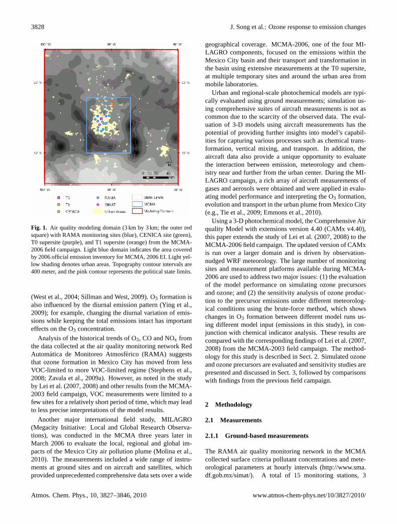
The Mexico City Metropolitan Area (MCMA), shown inFig. 1, is located in the Valley of Mexico. With nearly 20 mil-lion inhabitants, Mexico City is North America’s most popu-lous city and one of the largest megacities in the world. As aresult of rapid increase in population and urbanization, Mex-ico City suffers from serious air pollution problems (Molinaand Molina, 2002, 2004). The urban emissions also sig-nificantly influence air quality on the regional scale (Mena-Carrasco et al., 2009).

Ozone photochemical production is high in Mexico Citydue to high emissions of NOx, VOCs and CO, which pro-vide elevated radical sources, the driving force for urban pho-tochemical activity (Volkamer et al., 2007; Sheehy et al.,2008; Tie et al., 2009). Both measurements and chemicaltransport model simulations during the MCMA-2003 fieldmeasurement campaign (Molina et al., 2007) suggest thatO3 production in the source region is VOC limited duringthe photochemically active periods (Lei et al., 2007) andweakly dependent on meteorological conditions (Lei et al.,2008). Other recent studies (Tie et al., 2007; Torres-Jardon,2004) also suggest that O3 production in the MCMA is VOC-limited, in contrast to results of earlier modeling studies

Published by Copernicus Publications on behalf of the European Geosciences Union.

http://creativecommons.org/licenses/by/3.0/

3828 J. Song et al.: Ozone response to emission changes

39

Fig. 1. Air quality modeling domain (3 km by 3 km; the outer red square) with RAMA

monitoring sites (blue), CENICA site (green), T0 supersite (purple), and T1 supersite (orange) 5

from the MCMA-2006 field campaign. Light blue domain indicates the area covered by 2006

official emission inventory for MCMA, 2006 EI. Light yellow shading denotes urban areas.

Topography contour intervals are 400 meter, and the pink contour represents the political state

limits.

Fig. 1. Air quality modeling domain (3 km by 3 km; the outer redsquare) with RAMA monitoring sites (blue), CENICA site (green),T0 supersite (purple), and T1 supersite (orange) from the MCMA-2006 field campaign. Light blue domain indicates the area coveredby 2006 official emission inventory for MCMA, 2006 EI. Light yel-low shading denotes urban areas. Topography contour intervals are400 meter, and the pink contour represents the political state limits.

(West et al., 2004; Sillman and West, 2009). O3 formation isalso influenced by the diurnal emission pattern (Ying et al.,2009); for example, changing the diurnal variation of emis-sions while keeping the total emissions intact has importanteffects on the O3 concentration.

Analysis of the historical trends of O3, CO and NOx fromthe data collected at the air quality monitoring network RedAutomatica de Monitoreo Atmosferico (RAMA) suggeststhat ozone formation in Mexico City has moved from lessVOC-limited to more VOC-limited regime (Stephens et al.,2008; Zavala et al., 2009a). However, as noted in the studyby Lei et al. (2007, 2008) and other results from the MCMA-2003 field campaign, VOC measurements were limited to afew sites for a relatively short period of time, which may leadto less precise interpretations of the model results.

Another major international field study, MILAGRO(Megacity Initiative: Local and Global Research Observa-tions), was conducted in the MCMA three years later inMarch 2006 to evaluate the local, regional and global im-pacts of the Mexico City air pollution plume (Molina et al.,2010). The measurements included a wide range of instru-ments at ground sites and on aircraft and satellites, whichprovided unprecedented comprehensive data sets over a wide

geographical coverage. MCMA-2006, one of the four MI-LAGRO components, focused on the emissions within theMexico City basin and their transport and transformation inthe basin using extensive measurements at the T0 supersite,at multiple temporary sites and around the urban area frommobile laboratories.

Urban and regional-scale photochemical models are typi-cally evaluated using ground measurements; simulation us-ing comprehensive suites of aircraft measurements is not ascommon due to the scarcity of the observed data. The eval-uation of 3-D models using aircraft measurements has thepotential of providing further insights into model’s capabil-ities for capturing various processes such as chemical trans-formation, vertical mixing, and transport. In addition, theaircraft data also provide a unique opportunity to evaluatethe interaction between emission, meteorology and chem-istry near and further from the urban center. During the MI-LAGRO campaign, a rich array of aircraft measurements ofgases and aerosols were obtained and were applied in evalu-ating model performance and interpreting the O3 formation,evolution and transport in the urban plume from Mexico City(e.g., Tie et al., 2009; Emmons et al., 2010).

Using a 3-D photochemical model, the Comprehensive Airquality Model with extensions version 4.40 (CAMx v4.40),this paper extends the study of Lei et al. (2007, 2008) to theMCMA-2006 field campaign. The updated version of CAMxis run over a larger domain and is driven by observation-nudged WRF meteorology. The large number of monitoringsites and measurement platforms available during MCMA-2006 are used to address two major issues: (1) the evaluationof the model performance on simulating ozone precursorsand ozone; and (2) the sensitivity analysis of ozone produc-tion to the precursor emissions under different meteorolog-ical conditions using the brute-force method, which showschanges in O3 formation between different model runs us-ing different model input (emissions in this study), in con-junction with chemical indicator analysis. These results arecompared with the corresponding findings of Lei et al. (2007,2008) from the MCMA-2003 field campaign. The method-ology for this study is described in Sect. 2. Simulated ozoneand ozone precursors are evaluated and sensitivity studies arepresented and discussed in Sect. 3, followed by comparisonswith findings from the previous field campaign.

2 Methodology

2.1 Measurements

2.1.1 Ground-based measurements

The RAMA air quality monitoring network in the MCMAcollected surface criteria pollutant concentrations and mete-orological parameters at hourly intervals (http://www.sma.df.gob.mx/simat/). A total of 15 monitoring stations, 3

Atmos. Chem. Phys., 10, 3827–3846, 2010 www.atmos-chem-phys.net/10/3827/2010/

http://www.sma.df.gob.mx/simat/

http://www.sma.df.gob.mx/simat/

J. Song et al.: Ozone response to emission changes 3829

Table 1. VOC measurements during the MILAGRO campaign that were used in this study.

Site/Platform Analytical method VOCs used in the analysis Institution

CENICA GC-FID ethane, propane, acetylene, toluene, benzene, and xylene INE, MX

SIMAT EC-FOS Propene-equivalent olefins WSUGC and GC/MS ethane, ethene, propane, acetylene, toluene, benzene, xylene,

i-butene, 1-pentene, 1,3-butadiene, t-2-butene, c-2-butene, t-2-pentene, and c-2-pentene

UC Irvine

T0PTRMS acetaldehyde, toluene, and benzene Texas A&M U.DOAS benzene, toluene, o-xylene, m-xylene, p-xylene, phenol,

cresol, formaldehyde, and benzaldehydeMIT/ Univ. Heidelberg

QC-TILDAS and PTRMS formaldehyde, acetaldehyde, ethene, toluene, and benzene ARI

G-1 aircraft GC/PTRMS ethene, ethane, propane, benzene, toluene, xylenes, trimethyl-benzene; CO and O3 (non-VOCs)

BNL/PNNL

monitoring stations from each city sector (NE, NW, SE, SW,and CT), were selected based on the location representative-ness and data availability of CO, NOx, and O3 during thecampaign period. Measurements of NOx from RAMA usingthe chemiluminescence technique more accurately representgaseous NOy (West et al., 2004).

In this study, volatile organic compounds (VOCs) data re-ported during the MILAGRO Campaign were used to eval-uate the VOC emissions in the MCMA, particularly in theurban area. VOCs were measured at T0, T1, SIMAT andCENICA. Figure 1 shows the location of these sites. At T0,the urban supersite located just north of downtown MexicoCity, aldehydes and aromatics were measured with ProtonTransfer Reaction Mass Spectrometry (PTR-MS) (Zhao andZhang, 2004; Fortner et al., 2009), formaldehyde and aro-matics were measured with long-path Differential OpticalAbsorption Spectroscopy (DOAS); another set of formalde-hyde and ethene were acquired by quantum cascade tun-able infrared laser differential absorption spectrometry (QC-TILDAS) (Nelson et al., 2004) onboard the Aerodyne mobilelab while parked at T0; and canister samples of ethene, alka-nes, and aromatics were analyzed by Gas Chromatography(GC) and GC/MS. At the CENICA site, located in an urbancommercial/residential area with fewer industries than T0,alkanes and aromatics from canisters were speciated by GCanalysis using Flame Ionization Detection (GC-FID). At theSIMAT site (19◦24′ N, 99◦10′ W), close to the center of thecity, VOC concentrations and fluxes were measured usingeddy covariance (EC) techniques coupled with Fast OlefinSensor (FOS) (Velasco et al., 2009). Measurements at the T1site (de Gouw et al., 2009) located in the northeast urban out-skirt and other sites outside the MCMA were not included asthey are downwind sites, containing less information abouturban emissions. Table 1 lists the VOCs used in this studywith their corresponding measurement techniques and oper-ation institutions during the MCMA-2006 field campaign. A

detailed summary of the ground-based and aircraft measure-ments of VOCs can be found in Apel et al. (2010).

2.1.2 G-1 aircraft measurements

During MILAGRO-2006 several aircraft were deployed inand around the MCMA to collect chemical and meteorolog-ical data, including the G-1 operated by DOE (ftp://ftp.asd.bnl.gov/pub/ASP%20Field%20Programs/2006MAXMex/)and the C-130 operated by NCAR (http://mirage-mex.acd.ucar.edu/Measurements/C130/index.shtml). In this studyonly measurements from G-1 were included, since the flightscovered a smaller spatial and temporal domain, which is thescope of this study. There were 15 G-1 flights measuringchemical species over the MCMA, especially above T0and T1 supersites. Details on the G-1 aircraft flights overMexico City during MILAGRO are provided in Kleinmanet al. (2008) and Nunnermacker et al. (2008). Data used inthis study are 10-second average values for CO and O3 on7 March, and CO, O3 and speciated VOCs on 27 March. COand O3 were measured using VUV fluorescence analyzerand UV absorption detector, respectively (Springston et al.,2005). Canister samples of ethene, alkanes and aromat-ics were collected every 1–2 min, and analyzed by GC.Ten-second averaged aromatics were also measured withPTR-MS.

2.2 Model description

Concentrations of air pollutants were simulated using CAMxv4.40 (Environ, 2006) with the SAPRC99 chemical mecha-nism (Carter, 2000). CAMx simulates emission, advection,dispersion, chemical transformation and physical removalof air pollutants on an Eulerian 3-dimensional grid. The 6modeling episodes selected for this study are described inSect. 2.3 along with their meteorological classification. Agridded urban scale domain centering in Mexico City with

www.atmos-chem-phys.net/10/3827/2010/ Atmos. Chem. Phys., 10, 3827–3846, 2010

ftp://ftp.asd.bnl.gov/pub/ASP%20Field%20Programs/2006MAXMex/

ftp://ftp.asd.bnl.gov/pub/ASP%20Field%20Programs/2006MAXMex/

http://mirage-mex.acd.ucar.edu/Measurements/C130/index.shtml

http://mirage-mex.acd.ucar.edu/Measurements/C130/index.shtml


the resolution of 3 km, 70×70 grid cells was used in thisstudy (labeled as “modeling domain” in Fig. 1) with 16 ver-tical layers extending from the surface to about 7 km a.g.l.

Meteorological data inputs, including wind, tempera-ture, height/pressure, water vapor, vertical diffusivity, andclouds/precipitation, were derived from the Advanced Re-search WRF (ARW) model (WRF v2.2.1; Skamarock et al.,2005). The model simulations adopted three one-way nestedgrids with horizontal resolutions of 36, 12, and 3 km and 35sigma levels in the vertical direction. The grid cells used forthe three domains were 145×95, 259×160, and 193×193,respectively. The WRF model was initialized at 00:00 UTCevery day and integrated for 36 h. The physical parame-terization schemes included the modified Kain-Fritsch cu-mulus scheme (KF-Eta; Kain and Fritsch, 1993), the WRFSingle Moment (WSM) three-class microphysics (Hong etal., 2004), and the Yonsei State University (YSU) bound-ary layer scheme (Noh et al., 2003). National Centers forEnvironmental Prediction (NCEP) global final (FNL) analy-sis were used to create initial and boundary conditions. Toimprove the accuracy of the simulated fields, “observation-nudging”-based continuous four-dimensional data assimila-tion (FDDA) scheme (WRF-FDDA; Liu et al., 2005) wasemployed in the domain with a horizontal resolution of3 km. Multi-level upper-air observations were assimilated,including radar wind profilers, tethered balloon measure-ments, controlled meteorological balloon observations, air-craft observations, additional soundings inside the Mexicocity basin operated during the MILAGRO campaign, androutine soundings observations. The vertical diffusion coeffi-cients (kv) were reconstructed from the state variables of theWRF-FDDA output using the CMAQ scheme (Byun, 1999).According to de Foy et al. (2008), the CMAQ scheme over-estimates thekv values. These were therefore reduced to 30–40% as was done for the MCMA-2003 campaign (see Leiet al., 2008). This kv scaling has little influence on chemi-cal concentrations at nighttime and early morning (becauseof the patch treatment for the minimumkv values in the nearsurface layer), but it affects the day time concentrations (asmuch as 15% for surface CO) when there is active turbulentmixing.

Anthropogenic emissions used in the model were con-structed from the official emission inventory (EI) for theyear 2006 for the MCMA (http://www.sma.df.gob.mx/simat/programasambientales/anexo). The annual emissions inthe MCMA from different sources (mobile, area, and pointsource) were temporally resolved, chemically speciated, andthen spatially resolved into grid cells with a resolution of2.25 km. In areas outside the MCMA, official emissions datafrom point sources were available, but area and mobile emis-sions were not available. To account for these emissions,anthropogenic emissions outside the MCMA from the areaand mobile sources were estimated based on the populationdistribution as follows:

Ei,j = ri ×Ej,MCMA

PMCMA×SF (1)

where ri is population density in the grid cell obtainedfrom a high resolution population density map in theyear of 2005,Ej,MCMA and PMCMA are the total anthro-pogenic emissions of pollutant j and the population in theMCMA, respectively. SF are the population-based scal-ing factors that account for differences in emission inten-sities with respect to the MCMA, ranging linearly from0.1 to 0.3 forr < 200 heads/km2 (mainly rural areas) andr <15 000 heads/km2 (mainly urban areas with much higherproduction activities).

Lei et al. (2007, 2008) suggested that the overall VOCemissions in the official MCMA EI were underestimatedby 40% with variations among VOC species. Based onthe ground measurements made at CENICA site and at T0,adjustments were made to the emissions of lumped VOCsspecies (see Sect. 3.1 below). When the measurements wereunavailable, adjustment factors from the MCMA-2003 studywere used.

Biogenic emissions were estimated using the MEGANv2.04 model (Model of Emissions of Gases and Aerosolsfrom Nature) developed by Guenther et al. (2006, 2007).MEGAN uses land cover data with a high resolution (lessthan 1 km), emission factors specific to the interested re-gion, and time- and location-specific meteorological data.MEGAN estimates biogenic emissions as follows:

F = EF·γLAI ·γP ·γT ·γAGE (2)

whereF is the emission flux (µg m−2 hr−1), EF is the emis-sion factor at standard condition of 303 K (µg m−2 hr−1),γLAI , γP , γT , and γAGE are dimensionless scalars thatdescribe the response of emission to diurnal variation inleaf area index (LAI), photosynthetic photon flux density(PPFD), ambient temperature, and leaf age, respectively. Theemissions estimated from MEGAN on the spatial resolutionof 1 km were then lumped into the SAPRC99 species groups.

The chemical and boundary conditions were the same asthose used in the MCMA-2003 studies (Lei et al., 2007),which were constructed based on measurements, except theywere downscaled by about 10% considering a larger modeldomain used in this study.

2.3 Meteorological episodes

O3 production under different meteorological conditionswas examined. During MCMA-2003, three meteorologicalepisode types were identified (de Foy et al., 2005). O3-Southdays had a convergence zone in the south of the city thatmoved northwards into the early evening, causing high ozonepeaks in the south of the city. O3-North days had strongerwesterly winds aloft causing a convergence zone orientednorth-south through the city with pollutant exhaust to thenorth and high ozone peaks in the north. Cold Surge days


http://www.sma.df.gob.mx/simat/programas_ambientales/anexo

http://www.sma.df.gob.mx/simat/programas_ambientales/anexo


had strong cold and wet winds from the north flushing thebasin to the south, bringing rain and cloudiness with them.

During MILAGRO, six meteorological episode types wereidentified: the three episode types classified during MCMA-2003 (O3-South, O3-North and Cold Surge) applicable toMILAGRO, and extra three (O3-SV, O3-CnvS and O3-CnvN,see below) to account for meteorological conditions at the be-ginning and at the end of the campaign (de Foy et al., 2008).The first part of the campaign had dry northwesterly windsaloft with strong southward transport at the surface and noconvergence zones in the basin. These “South-Venting” dayshad clean air and rapid flushing of the urban plume to thesouth. The second part of the campaign was characterized byafternoon rains. These were classified into two subtypes de-pending on the location of the maximum amount of rainfall:convection-South and Convection-North. Convection takesplace when there are weak westerly winds aloft combinedwith humid conditions in the basin. Surface convergence inthe afternoon leads to convection and rainfall in the basinwith the location to the north or south dependent on the bal-ance of the winds from the plateau to the north and from thegap in the southeast. Cluster analysis of radiosonde profilesand surface wind measurements showed that conditions dur-ing MILAGRO were climatologically representative of thewarm dry season, suggesting that an analysis of O3 produc-tion during the different episodes of MILAGRO would berepresentative of general conditions in the basin for this sea-son (de Foy et al., 2008).

To minimize the influence from the transition of dif-ferent meteorological conditions on the selected episode,each episode was selected when at least 3 consecutive dayshad similar meteorological condition: 1–7 March 2006as O3-South Venting (O3-SV), 9–11 March 2006 as O3-North (O3-N1), 15–17 March 2006 as O3-South (O3-S), 18–20 March 2006 as O3-North (O3-N2), 24–26 March 2006 asO3-Convection South (O3-CnvS), and 27–30 March 2006 asO3-Convection North (O3-CnvN). O3-N1 was a period withflow towards the north and included one of the highest ozonedays (11 March), and the O3-N2 was a holiday period.

Mexico City was in the Central Standard Time zone at thetime of the campaign (CST=UTC−6); all results in this paperwill be reported in local time (LT=CST).

3 Results and discussions

Simulations of 1-h averaged ozone precursors and ozoneconcentrations using CAMx v4.40 were compared to mea-surements made during different meteorological episodes. Aday prior to each modeled episode was used for model “spin-up” to reduce the effects of chemical initial conditions, henceresults of these days are not included.

40

Fig. 2. Scatter plot of simulated and observed concentrations of (a) CO and (b) NOy averaged

over 15 RAMA monitoring sites during all episodes. Scatter plots only show datasets during

7:00-11:00 LT for CO and NOy. Performance statistics are also shown. The dashed lines indicate 5

a perfect positive correlation, and each color indicates a different meteorological episode.

Fig. 2. Scatter plot of simulated and observed concentrations of(a)CO and(b) NOy averaged over 15 RAMA monitoring sites dur-ing all episodes. Scatter plots only show datasets during 07:00–11:00 LT for CO and NOy. Performance statistics are also shown.The dashed lines indicate a perfect positive correlation, and eachcolor indicates a different meteorological episode.

3.1 Adjustment of emission inventory

For ozone precursors and ozone, simulations with the officialemission inventory were compared with the measurementstaken from 15 RAMA monitoring stations, the CENICA siteand the T0 supersite. Figure 2 shows that peak CO and NOyconcentrations were well simulated, with no mean fractionalbias and low fractional errors (see definitions below), sug-gesting that no adjustments to the emission inventory werenecessary for these species. Analysis of speciated VOC con-centrations suggested that emissions of most alkanes wereunderestimated by factors of 2–3 in mass except>C4 alka-nes (ALK4, ALK5 in the SAPRC99 speciation with OH rateconstant (kOH) of 5–10×103 and>1.0×103 ppm−1 min−1,respectively, mainly pentanes or higher alkanes). The num-ber of >C4 alkanes measured during MCMA-2006 cam-paign was not adequate for lumping, which did not allowus to perform measurement-model comparisons; the adjust-ment factors obtained during the MCMA-2003 study, 1.4and 0.6 for ALK4 and ALK5 respectively, were insteadused (Lei et al., 2007, 2008). The downscaling of ALK5emissions may be due also to their low concentrations andthe incomplete detection of these species by the GC-FIDmeasurement. Nevertheless the uncertainty in ALK5 emis-sions is not expected to substantially influence the O3 chem-istry due to their low concentrations and low VOC reac-tivity (Velasco et al., 2007). Ethylene (ETHE) emissionswere underestimated by 40% while emissions of other olefinswere overestimated by up to 50%. The emissions of aro-matics were overestimated by a factor of 2. It should benoted that the measurements of a limited number of aromaticspecies during the campaign were extrapolated to includemore species such that the observation-model comparisonsof lumped aromatics can be made (ARO1 are aromatics withkOH <2×104 ppm−1 min−1, consisting primarily of toluene,benzene and other monoalky benzenes, and ARO2 are aro-matics with kOH >2×104 ppm−1 min−1, mainly xylenes and



(Fig. 3)

Fig. 3. Comparisons of simulated and observed VOC concentrations after the emissions were adjusted.(a) ALK1, (b) ALK2, (c) ARO1,(d) ARO2 at CENICA, and(e) HCHO, (f) ETHE at T0. Measurements within 5 and 95 percentiles are included. Each colored dot indicatesindividual VOC measurement, and the solid line with corresponding color indicates the average of those measurements. Different colorindicates different measurement techniques: GC-FID data in black, DOAS data in light green, QC-TILDAS data in purple, GC and GC/MSdata in blue. Hourly averaged simulated VOC concentrations with±1 standard deviation (averaged over the time concurrent to the VOCobservations at CENICA and T0 in March 2006) are shown in red. Also shown are the agreement statistics (y=simulations,x=observations)during 6–11 a.m.

polyalkyl benezens). The extrapolation was derived fromthe MCMA-2003 canister data and DOAS measurements(Velasco et al., 2007; Volkamer et al., 2005; Lei et al.,2007). Also, emissions of aldehydes were underestimatedby factors of 3–4.5. Figure 3 compares VOC concentrationssimulated using emissions adjusted for the above underes-timates/overestimates with the observed values at CENICAand T0. The statistical metrics shown in the figure, meanfractional bias (MFB) and mean fractional error (MFE), aredefined as follows:

Mean fractional bias(MFB)

=1

N

N∑1

(pred−obs

(pred+obs)/

2

)×100% (3)

Mean fractional error(MFE)

=1

N

N∑1

(|pred−obs|

(pred+obs)/

2

)×100% (4)

whereN is the number of observations. In contrast withmean normalized bias (MNB) and mean normalized grosserror (MNGE) statistical metrics, MFB and MFE do not put



great emphasis on performance when observations are low(Boylan and Russell, 2006).

After the emissions were adjusted, the agreement betweensimulated and observed VOCs was within±1 standard devia-tion. It should be noted that some VOCs, for example HCHOand ETHE, measured concurrently and independently by dif-ferent groups at the same site showed large variations (Fig. 3eand f). The difference can be partially explained by thedifferent temporal coverage of the different measurementsand the spatial inhomogeneity. ARI mobile lab, where theQC-TILDAS measurement was taken, was stationed at T0on the ground∼50 m away from the T0 building whereasother ground measurements were sampled at the rooftop ofa building a few tens of meters a.g.l. This inhomogeneitycan cause the measurement difference of the primary speciesC2H4 shown in Fig. 3f. The moderate difference in HCHOshown in Fig. 3e is likely due to the fact that DOAS is a long-path measurement stationed at the building rooftop. Meanvalues of the measurements for these two lumped speciesby different groups were used for the emission adjustmentsof these species in our modeling. The post-adjusted ARO2emissions seem to be still underestimated by 15%.

The measurement data at SIMAT were not included dur-ing the emission adjustment process (they were not availablewhen we completed the model runs), instead they were usedto verify the adjustment. Figure 4 shows the comparisonof the simulated propene-equivalent olefin concentrations incompound with the FOS measurements. The propene equiva-lence here refers to the sensitivity response of the FOS instru-ment to olefin species with respect to propene (Velasco et al.,2009), which is different from the OH-reactivity based defi-nition introduced by Chameides et al. (1992). The simulatedeffective OLE concentrations were calculated from differentSAPRC99 OLE model species (ETHE, OLE1, OLE2 andISOP) weighted by their FOS response factors and their con-tributions to the standard VOC mixture used in the SAPRC99mechanism (Lei et al., 2009; Velasco et al., 2009). The goodagreement justifies the adjustment of olefin emissions.

A summary of total weekday emissions by source cate-gory in MCMA from 2006 official emission inventory andthe adjusted emissions are listed in Table 2. Overall, the VOCemissions from the official emission inventory were adjustedby 18–23% with the variability depending on the day-to-dayvariation in biogenic emissions. These variations are evenmore significant on the domain-wide emissions, leading tolarger variations in overall total VOC emissions. The totalVOC adjustment in the MCMA is smaller than the valueused by Lei et al. (2007, 2008) (1.26 vs. 1.65), probablydue to the VOC emissions changes over the years in boththe emission inventories and in actual emissions. Zavala etal. (2009b) find that the mobile emission factors of a fewVOC species (mainly aldehydes and aromatics) are reducedbetween 2003 and 2006 in the MCMA (by about 20%). Al-though the measured VOC species are only a small portion ofthe total VOCs, and the reported quantity is the emission fac-

0

10

20

30

40

50

60

70

80

0 2 4 6 8 10 12 14 16 18 20 22 24

Time (LT)

OLE

_eq

[ppb

v]

FOSCAMx

(Fig 4)

Fig. 4. Comparison of simulated (in red) and measured (in black)average diurnal variations of propene-equivalent olefin concentra-tions in compound at SIMAT. Error bars represent±1 standard de-viations, indicating the inter-diurnal variability. Data were averagedover 10–28 March 2006.

tor, it may be a strong indication of the emissions reductionof VOCs in 2006 compared to 2003. It should be noted thatthere are no sufficient VOC measurements available to reacha quantitative conclusion about the VOC emission changesbetween 2003 and 2006. The size of the VOC measurementdataset for evaluation and the variability in measurementsmay also contribute to the difference.

The adjusted emissions (base case) of CO, NOx and VOCsin the MCMA-2006 are 1990, 195 and 700–743 ktons/yr, re-spectively. Compared to those of MCMA-2003, which are1938, 183 and 900 ktons/yr (Lei et al., 2007, 2008), the NOxemissions increased slightly (6%), but the VOCs emissionsdecreased by about 20%, leading to changes in the NOx/VOCratio from 4.9 in 2003 to 3.7 (mass -based) in 2006. In par-ticular, the total emissions of highly reactive VOCs (alkenesand aromatics) decrease significantly (16% and 48%, respec-tively), resulting in the reduction of VOC reactivity in 2006compared to 2003. The larger decrease in the aromaticsemissions may also reflect the uncertainty of the method usedin the evaluation (e.g., the extrapolation) and indicates theneeds for further evaluations. These changes in NOx andVOCs and lower VOC reactivity in 2006 could affect thecharacteristics of ozone formation in the MCMA. For ex-ample, the lower VOC/NOx ratio and lower VOC reactivitymay contribute to the lower radical levels observed during theMCMA-2006 campaign compared to MCMA-2003 (Shirleyet al., 2006; Dusanter et al., 2009a, b).

3.2 Simulation of ozone precursors and ozoneconcentrations at surface

Before a model can be applied for O3 sensitivity studies it isessential to demonstrate its capability to accurately simulate



(Fig. 5)

(Tab 2)

2006 official EI Adjusted EI

VOCs Source CO NOx VOCs CO NOx Total OLE ARO

Area 5460 470 1160 5460 470 1520 - - Point 20 60 330 20 60 300 - - Biogenic 0 0 80 10 0 110-220 - - Total 5480 540 1570 5490

(12040) 540 (850)

1920-2040 (6440-7280)

106 126a

198 382a

a: Numbers in adjusted MCMA emissions in 2003.

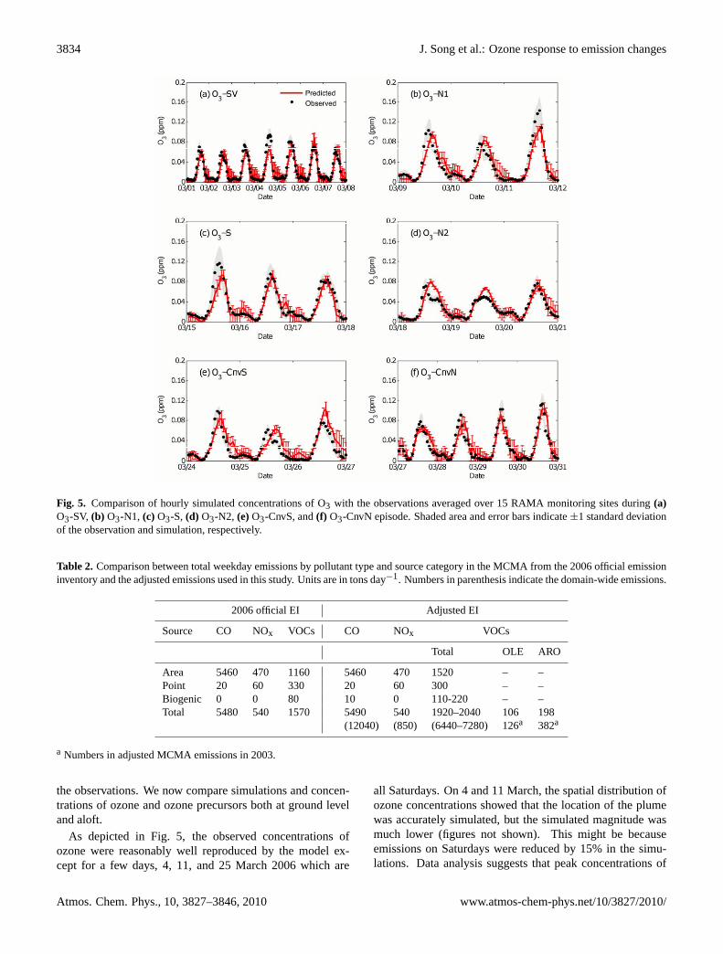
Fig. 5. Comparison of hourly simulated concentrations of O3 with the observations averaged over 15 RAMA monitoring sites during(a)O3-SV, (b) O3-N1, (c) O3-S, (d) O3-N2, (e)O3-CnvS, and(f) O3-CnvN episode. Shaded area and error bars indicate±1 standard deviationof the observation and simulation, respectively.

Table 2. Comparison between total weekday emissions by pollutant type and source category in the MCMA from the 2006 official emissioninventory and the adjusted emissions used in this study. Units are in tons day−1. Numbers in parenthesis indicate the domain-wide emissions.

2006 official EI Adjusted EI

Source CO NOx VOCs CO NOx VOCs

Total OLE ARO

Area 5460 470 1160 5460 470 1520 – –Point 20 60 330 20 60 300 – –Biogenic 0 0 80 10 0 110-220 – –Total 5480 540 1570 5490 540 1920–2040 106 198

(12040) (850) (6440–7280) 126a 382a

a Numbers in adjusted MCMA emissions in 2003.

the observations. We now compare simulations and concen-trations of ozone and ozone precursors both at ground leveland aloft.

As depicted in Fig. 5, the observed concentrations ofozone were reasonably well reproduced by the model ex-cept for a few days, 4, 11, and 25 March 2006 which are

all Saturdays. On 4 and 11 March, the spatial distribution ofozone concentrations showed that the location of the plumewas accurately simulated, but the simulated magnitude wasmuch lower (figures not shown). This might be becauseemissions on Saturdays were reduced by 15% in the simu-lations. Data analysis suggests that peak concentrations of



44

Fig. 6. Flight track of the G-1 aircraft on (a) 27 and (b) 7 March with starting, ending, and 5

sampling time stamps at each supersite from MCMA-2006 field campaign are shown; T0

(purple) and T1 (orange). Rainbow colors correspond to the measurement time. Topography

contour intervals are 400 meter. Letter A and B denote the location where flights passed multiple

times.

10

Fig. 6. Flight track of the G-1 aircraft on(a) 27 and(b) 7 March with starting, ending, and sampling time stamps at each supersite fromMCMA-2006 field campaign are shown; T0 (purple) and T1 (orange). Rainbow colors correspond to the measurement time. Topographycontour intervals are 400 m. Letter A and B denote the location where flights passed multiple times.

primary pollutants may be lower on Saturdays, but the over-all emissions may be similar to week days (Stephens et al.,2008; Stremme et al., 2009). On 25 March, the peak hourswere not captured by the model, which might be due to themeteorology.

Differences of ozone profiles during different meteorolog-ical episodes can be explained by different wind patterns andcharacteristics of each episode. As strong, dry and cleansoutherly winds flushed out the basin during South-Ventingdays, the observed ozone concentrations in the basin duringthese episodes were lower than those from other episodes(Fig. 5). During O3-S and O3-N1, on the other hand, pol-lutants accumulated in the south or north of the city whichled to high observed ozone concentrations. Although O3-N1and O3-N2 fell into the same meteorological episode cat-egory, the daily maximum ozone concentrations averagedover RAMA sites differed by 40% (107 ppb during O3-N1vs. 64 ppb during O3-N2 for episode-averaged peak ozone)mostly due to lower anthropogenic emissions (30–40% less)during the holiday period and also due to stronger southerlywinds during O3-N2 that vented the pollutants more effi-ciently. High O3 concentrations were still observed underthe convection conditions (O3-CnvS and O3-CnvN) becausethe convection usually occurred in the late afternoon.

As shown in Fig. 2, simulated morning hours (07:00–11:00 LT) concentrations of CO and NOy agreed well withthe observations. MFB and MFE during all the episodeswere 2% and 16% for CO and were 1% and 17% for NOy.The agreements of ozone for all the episodes were fairlygood with MFB and MFE values of−1% and 24%, re-spectively. Excluding weekend values, ozone concentrationsshowed better agreement with MFB and MFE values of−2%and 15%, respectively.

3.3 Comparisons with G-1 aircraft measurements

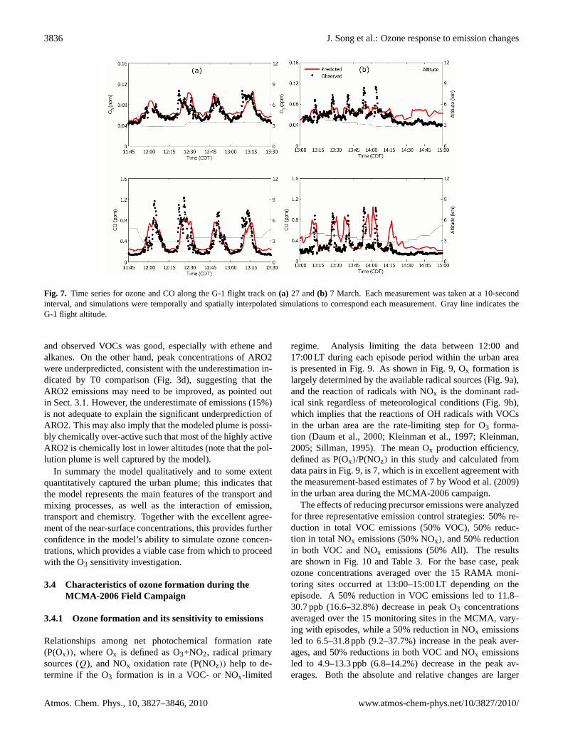
Two of the days when the G-1 aircraft flew over the urbanarea, 27 and 7 March, were selected as examples to comparethe CO and ozone concentrations aloft. Good agreement be-tween simulated and observed CO and O3 concentrations atthe surface (not shown) were obtained for both days. Figure 6shows the G-1 flight path on both days with the overpass timeat each supersite as well as starting and ending times of eachflight. On 27 March, classified as O3-CnvN, the flight fo-cused more on the northwestern MCMA and T1 supersiteand traversed an elevated pollutant plume four times (loca-tion “A” in Fig. 6a). Simulated concentrations were interpo-lated in time and space to the time and location of the dataalong the flight track. Figure 7 shows the comparisons ofO3 and CO. The agreement between the model and the ob-servations on 27 March was remarkably good, especially forO3, indicating the pollution plume was well captured by themodel. On 7 March, classified as O3-SV, the plane flew oversouthwestern MCMA 5 times (Location “B” in Fig. 6b) andcaptured the high CO and O3 concentrations between 13:06and 14:09 LT. The measured plume width was about 15 km,whereas the simulated plume was about 28 km wide, whichresulted in lower and longer-lasting elevated concentrationsfor both CO and O3 (Fig. 7b). Although quantitatively speak-ing the model did not simulate well the magnitude and widthof the plume, qualitatively it captured both the location andthe peak time. This was representative of other days wherethe simulated urban plumes were in qualitative agreementwith the observations

The aircraft measurements on 27 March also providedspeciated VOC data for further model evaluation. Figure 8shows the comparison of simulated VOCs and observationsalong with the flight path. Agreement between simulated



45

Fig. 7. Time series for ozone and CO along the G-1 flight track on (a) 27 and (b) 7 March. Each

measurement was taken at a 10-second interval, and simulations were temporally and spatially 5

interpolated simulations to correspond each measurement. Gray line indicates the G-1 flight

altitude.

Fig. 7. Time series for ozone and CO along the G-1 flight track on(a) 27 and(b) 7 March. Each measurement was taken at a 10-secondinterval, and simulations were temporally and spatially interpolated simulations to correspond each measurement. Gray line indicates theG-1 flight altitude.

and observed VOCs was good, especially with ethene andalkanes. On the other hand, peak concentrations of ARO2were underpredicted, consistent with the underestimation in-dicated by T0 comparison (Fig. 3d), suggesting that theARO2 emissions may need to be improved, as pointed outin Sect. 3.1. However, the underestimate of emissions (15%)is not adequate to explain the significant underprediction ofARO2. This may also imply that the modeled plume is possi-bly chemically over-active such that most of the highly activeARO2 is chemically lost in lower altitudes (note that the pol-lution plume is well captured by the model).

In summary the model qualitatively and to some extentquantitatively captured the urban plume; this indicates thatthe model represents the main features of the transport andmixing processes, as well as the interaction of emission,transport and chemistry. Together with the excellent agree-ment of the near-surface concentrations, this provides furtherconfidence in the model’s ability to simulate ozone concen-trations, which provides a viable case from which to proceedwith the O3 sensitivity investigation.

3.4 Characteristics of ozone formation during theMCMA-2006 Field Campaign

3.4.1 Ozone formation and its sensitivity to emissions

Relationships among net photochemical formation rate(P(Ox)), where Ox is defined as O3+NO2, radical primarysources (Q), and NOx oxidation rate (P(NOz)) help to de-termine if the O3 formation is in a VOC- or NOx-limited

regime. Analysis limiting the data between 12:00 and17:00 LT during each episode period within the urban areais presented in Fig. 9. As shown in Fig. 9, Ox formation islargely determined by the available radical sources (Fig. 9a),and the reaction of radicals with NOx is the dominant rad-ical sink regardless of meteorological conditions (Fig. 9b),which implies that the reactions of OH radicals with VOCsin the urban area are the rate-limiting step for O3 forma-tion (Daum et al., 2000; Kleinman et al., 1997; Kleinman,2005; Sillman, 1995). The mean Ox production efficiency,defined as P(Ox)/P(NOz) in this study and calculated fromdata pairs in Fig. 9, is 7, which is in excellent agreement withthe measurement-based estimates of 7 by Wood et al. (2009)in the urban area during the MCMA-2006 campaign.

The effects of reducing precursor emissions were analyzedfor three representative emission control strategies: 50% re-duction in total VOC emissions (50% VOC), 50% reduc-tion in total NOx emissions (50% NOx), and 50% reductionin both VOC and NOx emissions (50% All). The resultsare shown in Fig. 10 and Table 3. For the base case, peakozone concentrations averaged over the 15 RAMA moni-toring sites occurred at 13:00–15:00 LT depending on theepisode. A 50% reduction in VOC emissions led to 11.8–30.7 ppb (16.6–32.8%) decrease in peak O3 concentrationsaveraged over the 15 monitoring sites in the MCMA, vary-ing with episodes, while a 50% reduction in NOx emissionsled to 6.5–31.8 ppb (9.2–37.7%) increase in the peak aver-ages, and 50% reductions in both VOC and NOx emissionsled to 4.9–13.3 ppb (6.8–14.2%) decrease in the peak av-erages. Both the absolute and relative changes are larger



46

Fig. 8. Time series for VOCs on 27 March are shown. Canister measurements were collected

within 1-2 minutes (blue dots), and real-time VOCs analyzed by PTRMS were taken at 10-

second intervals (black dots). Simulations were temporally and spatially interpolated to

correspond to each measurement. 5

Fig. 8. Time series for VOCs on 27 March are shown. Canister measurements were collected within 1–2 min (blue dots), and real-timeVOCs analyzed by PTRMS were taken at 10-s intervals (black dots). Simulations were temporally and spatially interpolated to correspondto each measurement.

Table 3. Percentage changes of episode averaged peak ozone concentrations due to emission reductions under different meteorologicalconditions.

Episode Base case O3 (ppb) 50% VOC (%) 50% NOx (%) 50% All (%)

O3-SV 66.9 −24.5 36.3 −8.1O3-N1 93.5 −32.8 18.4 −14.2O3-S 84.3 −34.2 37.7 −7.5O3-N2 70.9 −16.6 9.2 −6.9O3-CnvS 80.4 −26.9 14.7 −9.3O3-CnvN 78.0 −23.7 23.6 −6.8

than obtained during MCMA-2003 (Lei et al., 2007, 2008),mainly due to the changes in estimated VOC emissions. Theozone concentrations from 50% VOC followed the trend ofthe base case in the early morning and late afternoon; how-ever, daytime ozone concentrations were significantly lowerthan those from the base case. Also, peak ozone concen-trations from 50% VOC reduction generally occurred 1–2 hlater than those from the base case. On the other hand,NOx reductions produced significant increases in peak ozonethroughout the day, and peak ozone concentrations occurred

1–2 h earlier than those from the base case. Reductions inboth VOC and NOx emissions generally followed the trendof the base case during the daytime with changes in episode-averaged daily maximum 1-h ozone concentrations (4.9 ppbdecrease from O3-N2 to 13.3 ppb decrease from O3-N1), butfollowed the trend of 50% NOx in the early morning and lateafternoon. These results indicate that the O3 formation isVOC-sensitive in the MCMA urban area.

During different meteorological episodes, the magnitudeof changes, as well as the peak ozone timing was different



47

5

Fig. 9. Indicators examining the VOC- or NOx-limited conditions for urban area during 12:00-

17:00 LT; Relationships between primary radical production rates and (a) Ox formation rate and

(b) NOx oxidation rate

Fig. 9. Indicators examining the VOC- or NOx-limited conditionsfor urban area during 12:00–17:00 LT; Relationships between pri-mary radical production rates and(a) Ox formation rate and(b)NOx oxidation rate.

for different emission control scenarios, with the largestchanges in the O3-S episode and the smallest changes dur-ing the convection events. These results suggest that theMCMA urban region is VOC-limited during the ozone peakhours as well as during the morning and late afternoon. Un-der VOC-limited conditions, ozone formation is limited bythe amount of available radicals for NO→NO2 conversion(RO2/HO2+NO→RO/OH+NO2) that eventually leads to O3production. Meanwhile NO2 –radical reactions become thedominant radical chemical sink. These findings are consis-tent with results from the MCMA-2003 field campaign (Leiet al., 2007, 2008; Volkamer et al., 2007; Sheehy et al., 2008)as well as with MILAGRO measurement-based conclusions(Nunnermacker et al., 2008; Wood et al., 2009; Stephens etal., 2008).

Figure 11 shows the spatial distribution of changes inpeak ozone concentrations due to reductions in emissions ofVOCs, NOx, and both during each meteorological episode.Compared to the base case, 50% reductions in VOC emis-sions led to domain-wide decrease in ozone concentrations,up to 55.8 ppb with maximum decreases in the high ozoneareas (Fig. 11b). This is always the case with few exceptionsin polluted urban atmosphere because of high NOx, limitedradicals and the magnitude of VOC emissions reduction. Incontrast, 50% reductions in NOx emissions led to either in-creases or decreases in peak ozone concentrations, depend-ing on the location (Fig. 11c). In the urban area, ozone con-centrations increased by up to 56.3 ppb due to the reductionsin NOx emissions while they decreased in mountain/rural ar-eas. The spatial distributions of changes in ozone concentra-tions were also sensitive to the direction of the plume, whichwas highly dependent on the meteorological episode. Whenboth VOC and NOx emissions were reduced, ozone concen-trations in the urban area either increase or decrease depend-ing on the direction of the plume (Fig. 11d). For example,ozone concentrations at peak hours during O3-N1 decreasedby up to 26.0 ppb in the urban area when both VOC and NOxemissions were reduced; however, the concentration at the

same location increased by up to 6.9 ppb during O3-CnvS.This also suggests that ozone formation in the MCMA urbanarea is VOC-sensitive.

3.4.2 Indicator (PH2O2/PHNO3) analysis

Due to its robust theoretical backgrounds, a strong correla-tion between its constant ratio and the P(Ox) ridgeline andthe least uncertainty, the ratio of the production rates ofhydrogen peroxide and nitric acid (PH2O2/PHNO3) has beenwidely used in chemical indicator analysis to examine thesensitivity of ozone formation (Sillman, 1995; Tonnesen andDennis, 2000). It has been established in many urban ar-eas in North America that if the PH2O2/PHNO3 ratio is higherthan 0.35, it is defined as NOx-limited regime; if the ratiois lower than 0.06, it is defined as VOC-limited regime, andin between it is defined as a transition regime (Tonnesen andDennis, 2000). Figure 12a depicts the relationships betweenP(Ox) and PH2O2/PHNO3 at 12:00–17:00 LT under two differ-ent emission reduction scenarios: 50% VOC and 50% NOx.Here we define the transition regime as the situation wherethe difference in the O3 production rate between the twoemission scenarios is less than 5% relative to the base case.This definition is similar to the one defined by Sillman (1999)in the context of urban O3 chemistry. By this definition,ozone formation in the MCMA is NOx-limited when thePH2O2/PHNO3 ratio is higher than 0.24, VOC-limited whenthe ratio is lower than 0.14, and transitional when the ra-tio is between 0.14 and 0.24, and it varies little with dif-ferent meteorological conditions. These results are withinthe criteria that were specified from previous studies (Ton-nesen and Dennis, 2000). Note that Fig. 12a encompassesall the episodes including weekends (shown in gray). Mostgray data points overlapped with other data points, indicatingthat the relationship between P(Ox) and PH2O2/PHNO3 duringweekends is similar to the one during weekdays.

The PH2O2/PHNO3 criteria were applied to examine the spa-tial distribution of VOC and NOx limitations. Figure 12bgives an example of the PH2O2/PHNO3 spatial variation on 7and 27 March, two days with a high percentage of VOC-and NOx-limited regime, respectively. As shown in the fig-ure, there is a large variation in the spatial distributions ofVOC- or NOx-limited regime in the afternoon among dif-ferent meteorological episodes: ozone formation in the highNOx emitting urban areas are sensitive to VOC, whereas theozone formations in the mountains or low NOx emitting ruralareas are more sensitive to NOx, i.e., ozone formations in theurban area are VOC-limited regardless of the meteorologicalepisodes; however, in areas outside the city with relativelylow-NOx emissions it can be either NOx- or VOC-limitedregime depending on the meteorological episode. In terms ofthe urban area, controlling VOCs would be a more effectiveway to reduce ozone concentrations than controlling NOx;however, it is essential to understand that the sensitivity ofVOC- or NOx-limited regime changes over time and space.



48

Fig. 10. Time series showing the sensitivity of ozone production to ozone precursors under

different meteorological conditions, compared to the base case. Data were averaged over 15

RAMA monitoring stations and over each period. Black line indicates the base case, red

indicates the ozone concentrations with 50% reductions in VOC emissions, blue indicates those 5

with 50% reductions in NOx emissions, and gray indicates those with 50% reductions in both

VOC and NOx emissions.

Fig. 10.Time series showing the sensitivity of ozone production to ozone precursors under different meteorological conditions, compared tothe base case. Data were averaged over 15 RAMA monitoring stations and over each period. Black line indicates the base case, red indicatesthe ozone concentrations with 50% reductions in VOC emissions, blue indicates those with 50% reductions in NOx emissions, and grayindicates those with 50% reductions in both VOC and NOx emissions.

3.4.3 NOx-VOC sensitivity vs. chemical aging

Lei et al. (2007, 2008) show that the O3 sensitivity in theMCMA is closely related to chemical aging (NOz/NOy) ofthe urban plume, and point out that as the plume becomeschemically aged, the O3 formation tends to shift from VOC-limited to NOx-limited, but no criteria have been establishedfor the transition. In this study, we attempt to establish thecriteria by analyzing the P(Ox)-NOz/NOy relationship underdifferent emissions, in order to use measurements to assessthe O3 formation regime. Although both the O3-chemicalaging relationship and the P(H2O2)/P(HNO3) relation dis-cussed above attempt to use measurements to assess the O3

formation characteristics, they are different in that the formeris derived from the radical chemistry and reflects the in situchemistry while the latter is usually associated with plumedilution and transport and is embedded with the plume his-tory.

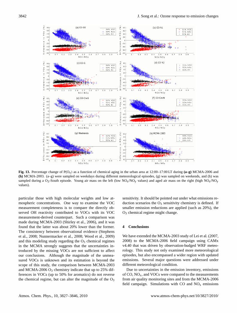
Figure 13 illustrates the percentage change in P(Ox)

(1P(Ox)) as a function of base case NOz/NOy at 12:00–17:00 LT in the MCMA urban region under different mete-orological conditions during the MILAGRO campaign whenemissions are reduced by 50%. Figure 13a–f shows thechange on weekdays while Fig. 13g shows the change duringweekends. We find that1P(Ox) generally decreases with in-creasing chemical aging and shifts from positive to negative



49

O3-SV O3-N1 O3-S O3-N2 O3-CnvS O3-CnvN

5

(a)

(b)

(c)

(d)

Fig. 11. Spatial distribution of peak ozone changes due to the changes in emissions under different meteorological conditions.(a) Peakozone concentration in the base case,(b) ozone change with 50% VOC,(c) ozone change with 50% NOx, and(d) ozone change with 50%VOC and NOx. Snapshots were taken at peak ozone hours, units are in ppm.

when the NOx emissions are reduced by 50%,1P(Ox) in-creases gradually with increasing NOz/NOy when the VOCemissions are reduced by 50%, while1P(Ox) remains con-stant with NOz/NOy when emissions of both NOx and VOCsare reduced by 50%. These characteristics are consistentunder different meteorological conditions, and no notice-able differences are found between weekdays and week-ends. Furthermore, it can be established that O3 forma-tion is VOC-limited when NOz/NOy <0.45, but is NOx-limited when NOz/NOy >0.60, with the latter occurring sig-nificantly less frequently. It should be noted that these crite-ria may change with location and with different base emis-sions. For example, a Lagrangian-wise analysis by Lei etal. (2008) shows that the urban plume becomes NOx-limitedwhen NOz/NOy >0.8 after the plume travels outside of theMCMA urban area during the MCMA-2003 campaign.

The O3 sensitivity is discussed above in the context ofemissions and chemical aging represented by NOz/NOy. Infact, O3 sensitivity is also influenced by several other factors(Sillman, 1999), such as VOC/NOx ratio, VOC reactivity andthe severity of the event (including dilution). Although theratio of NOz/NOy is used to represent the chemical aging, itis often affected by emissions, since the level of NOy reflectsthe NOx emissions (and mixing) and NOz is affected by rad-ical concentrations, which in turn are affected by both VOCs

and NOx. In addition, the chemical aging is usually accom-panied by the process of dilution, which alone can shift theNOx-VOC sensitivity to the VOC-limited regime (Milfordet al., 1994; Sillman, 1999). Milford et al. (1994) foundthat for plumes with same VOC/NOx emission ratios, plumeswith higher NOx emissions tend to be more VOC-limited,and plumes with lower NOx emissions tend to become NOx-limited more quickly as they are photochemically processed.Therefore it should be noted that when discussing the O3chemistry – chemical aging relationship, many other phys-ical and chemical processes are often inevitably involved.

3.5 Comparison of findings with the MCMA-2003 FieldCampaign

During MCMA-2003 field campaign, Lei et al. (2007, 2008)investigated the relationships between ozone production rate,radical primary source, and VOC-to-NO2 reactivity usingidentical or similar model (an older version in the 2007 pa-per), finding that the urban core area was VOC-limited dur-ing the O3-South, Cold-Surge, and O3-North episodes. Thiswas further analyzed by the simulations using three differ-ent emissions control strategies. Similar findings are ob-tained during the MCMA-2006 field campaign under dif-ferent meteorological conditions. However, the degree of



(a)

51

(a)

(b)

5

Fig. 12. (a) The percentage change in Ox formation rate as a function of the indicator, ratio of

H2O2 production rate to HNO3 production rate at 12:00-17:00 LT during the episodes (weekends

are shown in gray) within the urban area. The dashed bars envelop the transition regime. (b)

Spatial distribution of the ratio at 14:00 LT on 7 and 27 March indicating the NOx-VOC 10

sensitivity. Topography contour intervals are 400 meter.

(b)

51

(a)

(b)

5

Fig. 12. (a) The percentage change in Ox formation rate as a function of the indicator, ratio of

H2O2 production rate to HNO3 production rate at 12:00-17:00 LT during the episodes (weekends

are shown in gray) within the urban area. The dashed bars envelop the transition regime. (b)

Spatial distribution of the ratio at 14:00 LT on 7 and 27 March indicating the NOx-VOC 10

sensitivity. Topography contour intervals are 400 meter.

Fig. 12. (a)The percentage change in Ox formation rate as a function of the indicator, ratio of H2O2 production rate to HNO3 production rateat 12:00–17:00 LT during the episodes (weekends are shown in gray) within the urban area. The dashed bars envelop the transition regime.(b) Spatial distribution of the ratio at 14:00 LT on 7 and 27 March indicating the NOx-VOC sensitivity. Topography contour intervals are400 m.

the VOC-limitation increases as shown in Figs. 10 and 13.The 1P(Ox)-NOx relationship shown in Fig. 14 also in-dicates that the transition area between VOC-sensitive andNOx-sensitive regimes is much more narrow and shifts tolower NOx levels in MCMA-2006 compared to the MCMA-2003, and the relationship for the NOx-reduction case is moremonotonic. These illustrate that O3 formation in the ur-ban area during the MCMA-2006 is more VOC-limited. Weattribute the difference in the degree of VOC-limitation tothe chemistry . Meteorologically, Shaw et al. (2007) evalu-ated the vertical mixing during MILAGRO and found it tobe similar to prior studies. de Foy et al. (2008) found thatMarch 2006 was climatologically representative of the warmdry season. Compared with April 2003, there were fewerwet days and more warm winds from the south but overallthe transport patterns were similar. The difference is prob-ably mainly due to the reduced VOC reactivity and lowerVOCs in the estimated emissions in 2006, as indicated by the

overall∼20% decrease in VOC emissions and significant de-creases in emissions of reactive alkenes and aromatics. The6% increase of NOx emissions can also contribute to the ten-dency, but probably with a minor impact due to the moderateincrease. Although not shown in Fig. 14 (because almostall weekend data points would be overlapped with the week-days counterparts), the O3 formation response to the emis-sion change on weekends is very similar to that of weekdays,consistent with the results using P(H2O2)/P(HNO3) ratio asindicator.

The comparison between the MCMA-2003 and MCMA-2006 O3 chemistry allow us to estimate, to a certain extent,how emissions uncertainties may affect the conclusions ofthis study. Our model-based evaluation of VOC emissions re-lies on the assumption that the observations contain the fullspectrum of the lumped model species such that the com-parison can be made. However, it is likely that some VOCcompounds are missed by the measurement techniques, in



52

Fig. 13. Percentage change of P(Ox) as a function of chemical aging in the urban area at 12-17

LT during (a)-(g) MCMA-2006 and (h) MCMA-2003. (a)-(g) were sampled on weekdays during

different meteorological episodes, (g) was sampled on weekends, and (h) was sampled during a

O3-South episode. Young air mass on the left (low NOz/NOy values) and aged air mass on the

right (high NOz/NOy values).

Fig. 13. Percentage change of P(Ox) as a function of chemical aging in the urban area at 12:00–17:00 LT during(a–g)MCMA-2006 and(h) MCMA-2003. (a–g) were sampled on weekdays during different meteorological episodes, (g) was sampled on weekends, and (h) wassampled during a O3-South episode. Young air mass on the left (low NOz/NOy values) and aged air mass on the right (high NOz/NOyvalues).

particular those with high molecular weights and low at-mospheric concentrations. One way to examine the VOCmeasurement completeness is to compare the directly ob-served OH reactivity contributed to VOCs with its VOCmeasurement-derived counterpart. Such a comparison wasmade during MCMA-2003 (Shirley et al., 2006), and it wasfound that the latter was about 20% lower than the former.The consistency between observational evidence (Stephenset al., 2008; Nunnermacker et al., 2008; Wood et al., 2009)and this modeling study regarding the O3 chemical regimesin the MCMA strongly suggests that the uncertainties in-troduced by the missing VOCs are not sufficient to affectour conclusions. Although the magnitude of the unmea-sured VOCs is unknown and its estimation is beyond thescope of this study, the comparison between MCMA-2003and MCMA-2006 O3 chemistry indicate that up to 25% dif-ferences in VOCs (up to 50% for aromatics) do not reversethe chemical regime, but can alter the magnitude of the O3

sensitivity. It should be pointed out under what emissions re-duction scenarios the O3 sensitivity chemistry is defined. Ifsmaller emission reductions are applied (such as 20%), theO3 chemical regime might change.

4 Conclusions

We have extended the MCMA-2003 study of Lei et al. (2007,2008) to the MCMA-2006 field campaign using CAMxv4.40 that was driven by observation-budged WRF meteo-rology. This study not only examined more meteorologicalepisodes, but also encompassed a wider region with updatedemissions. Several major questions were addressed underdifferent meteorological condition.

Due to uncertainties in the emission inventory, emissionsof CO, NOx, and VOCs were compared to the measurementsfrom air quality monitoring sites and from the MCMA-2006field campaign. Simulations with CO and NOx emissions



53

(a) MCMA-2006 (b) MCMA-2003

Fig. 14. Simulated percentage change of P(Ox) as a function of base case NOx in the urban area

at 12-17 LT during (a) MCMA-2006 and (b) MCMA-2003. Datapoints in (a) include weekdays 5

only throughout the whole episode.

Fig. 14. Simulated percentage change of P(Ox) as a function of base case NOx in the urban area at 12:00–17:00 LT during(a) MCMA-2006and(b) MCMA-2003. Datapoints in (a) include weekdays only throughout the whole episode.

from the official 2006 emission inventory agreed well withthe observations, while emissions of speciated VOCs re-quired further adjustments. Overall, total VOC emissionswere underestimated by 18–23% which is much smaller thanthe results found in Lei et al. (2007, 2008), with significantdecreases in the OH reactivities of alkenes and aromatics.With adjusted emissions, simulated ozone precursors andozone concentrations were compared to observations froma variety of measurements, including surface measurementsand aircraft measurements, under different meteorologicalepisodes. Except for a few days, the observed concentrationsof ozone and ozone precursors at the surface were reason-ably well reproduced by the model. The peaks from aircraftmeasurements were also well predicted by the model. Thecombination of surface and aircraft measurements allow theevaluation of the simulated vertical distribution of CO, VOC,and O3 concentrations as well as an evaluation of the localemission inventory.

To determine the relative benefits of VOC and NOx con-trols, we have examined the relationships among net photo-chemical formation rates, radical primary sources, and NOxoxidation rates in the MCMA urban area. We also have ex-amined the ratio of the production rates of hydrogen per-oxide and nitric acid, PH2O2/PHNO3 in the urban area andmountain/rural areas. Within the urban area, Ox formationwas largely determined by the radical sources available, andthe reaction of radicals with NOx represented the dominantradical sink, which implied that the urban area is VOC-sensitive regardless of meteorological conditions. This wasalso shown from the spatial distribution of PH2O2/PHNO3. Incontrast, ozone formation in the mountain areas or low NOxemitting rural areas was mostly NOx-limited depending onmeteorological conditions.

We have also examined the sensitivities of ozone produc-tion to precursor emissions during the MCMA-2006 fieldcampaign. Independent of different meteorological episodes,reductions in VOC emissions always led to unanimous de-crease in ozone concentrations, as the case in most pollutedurban atmospheres. In contrast, reductions in NOx emis-

sions led to large increases in the urban area and decreasesin mountain/rural areas. However, spatial distributions ofchanges in ozone concentrations were highly sensitive to themeteorological episode. This was more evident when bothVOC and NOx emissions were reduced because ozone con-centrations in the urban area experienced both increase anddecrease depending on the direction of the plume.

Overall, ozone formation in the urban core area was VOC-limited under different meteorological episodes, while thesurrounding areas with relatively low-NOx emissions canbe either NOx- or VOC-limited regime depending on theepisode. Our results from MCMA-2006 suggest that the con-trols on VOC emissions would be a more effective way toreduce ozone concentrations in the urban area, which is con-sistent with our previous results from the MCMA-2003 fieldcampaign. However, the degree of VOC-limitation increasedfor MCMA-2006 due to reduced VOCs, reduced VOC reac-tivity and moderately higher NOx emissions in the estimatedemissions. Furthermore, meteorological conditions led tolarge variations in regime for the relatively low-NOx emit-ting area, implying that emission controls would depend onlocation and meteorology.

In this study we did not include the biomass burning emis-sions. It is well known that biomass burning emissions areimportant contributor to the O3 precursor and PM emissions,and can significantly affect O3 levels and PM loading in theMCMA, even though their contributions ate highly uncertain(e.g., Yokelson et al., 2007, 2009; Moffet et al. , 2008; Stoneet al., 2008, etc.). The effect of biomass burning on O3 for-mation (and PM) and its sensitivity in the MCMA and itssurroundings is an important issue, and we plan to address itin future study.

Acknowledgements.We are indebted to the large number of peopleinvolved in the MILAGRO campaign as well as those involvedin long-term air quality monitoring and the emissions inventoryin the Mexico City metropolitan area, which made this studypossible. In particular, we are grateful to Christine Wiedinmyerfor her assistance with the MEGAN simulations, the Governmentof the Federal District for providing point emissions data outside



of the MCMA; the researchers from the University of Californiaat Irvine, Aerodyne Research Inc., Washington State University,BNL and PNNL for making their data available to constrain ourchemical transport model. We thank Ezra Wood for his valuablediscussions on the ARI QC-TILDAS measurements. The authorsalso acknowledge the anonymous reviewers for their valuablecomments, which helped to improve the quality of this article.The WRF computer time was provided by the National Center forAtmospheric Research, which is sponsored by the National ScienceFoundation. This work was supported by the US Department ofEnergy’s Atmospheric Sciences Program (DE-FG02-05ER63980),the US National Science Foundation’s Atmospheric ChemistryProgram (ATM-0528227 and ATM-810931), Mexico’s ComisionAmbiental Metropolitana and the Molina Center for Energy andthe Environment.

Edited by: S. Madronich

References

Apel, E. C., Emmons, L. K., Karl, T., Flocke, F., Hills, A. J.,Madronich, S., Lee-Taylor, J., Fried, A., Weibring, P., Walega, J.,Richter, D., Tie, X., Mauldin, L., Campos, T., Weinheimer, A.,Knapp, D., Sive, B., Kleinman, L., Springston, S., Zaveri, R., Or-tega, J., Voss, P., Blake, D., Baker, A., Warneke, C., Welsh-Bon,D., de Gouw, J., Zheng, J., Zhang, R., Rudolph, J., Junkermann,W., and Riemer, D. D.: Chemical evolution of volatile organiccompounds in the outflow of the Mexico City Metropolitan area,Atmos. Chem. Phys., 10, 2353–2375, 2010,http://www.atmos-chem-phys.net/10/2353/2010/.

Boylan, J. W. and Russell, A. G.: PM and light extinction modelperformance metrics, goals, and criteria for three-dimensional airquality models, Atmos. Environ., 40, 4946–4959, 2006.

Byun, D. W.: Dynamically consistent formulations in meteorolog-ical and air quality models for multiscale atmospheric studies.Part I: Governing equations in a generalized coordinate system,J. Atmos. Sci., 56, 3789–3807, 1999.

Carter, W.: Implementation of the SAPRC-99 chemical mechanisminto the Models-3 framework. Report to the United States En-vironmental Protection Agency,http://www.cert.ucr.edu/∼carter/absts.htm#s99mod3, 29 January 2000.

Chameides, W. L., Fehsenfeld, F., Rodgers, M. O., Cardelino, C.,Martinez, J., Parrish, D., Lonneman, W., Lawson, D. R., Ras-mussen, R. A., Zimmerman, P., Greenberg, J., Mlddleton, P., andWang, T.: Ozone Precursor Relationships in the Ambient Atmo-sphere, J. Geophys. Res., 97(D5), 6037–6055, 1992.

Daum, P. H., Kleinman, L., Imre, D. G., Nunnermacker, L. J., Lee,Y.-N., Springston, S. R., Newman, L., and Weinstein-Llyod, J.:Analysis of the processing of Nashville urban emission on July3 and July 18, 1995, J. Geophys. Res., 105, 9155–9164, 2000.

de Gouw, J. A., Welsh-Bon, D., Warneke, C., Kuster, W. C., Alexan-der, L., Baker, A. K., Beyersdorf, A. J., Blake, D. R., Cana-garatna, M., Celada, A. T., Huey, L. G., Junkermann, W., Onasch,T. B., Salcido, A., Sjostedt, S. J., Sullivan, A. P., Tanner, D.J., Vargas, O., Weber, R. J., Worsnop, D. R., Yu, X. Y., andZaveri, R.: Emission and chemistry of organic carbon in thegas and aerosol phase at a sub-urban site near Mexico City inMarch 2006 during the MILAGRO study, Atmos. Chem. Phys.,

9, 3425–3442, 2009,http://www.atmos-chem-phys.net/9/3425/2009/.

de Foy, B., Caetano, E., Magana, V., Zitacuaro, A., Cardenas, B.,Retama, A., Ramos, R., Molina, L. T., and Molina, M. J.: MexicoCity basin wind circulation during the MCMA-2003 field cam-paign, Atmos. Chem. Phys., 5, 2267–2288, 2005,http://www.atmos-chem-phys.net/5/2267/2005/.

de Foy, B., Fast, J. D., Paech, S. J., Phillips, D., Walters, J. T.,Coulter, R. L., Martin, T. J., Pekour, M. S., Shaw, W. J., Kasten-deuch, P. P., Marley, N. A., Retama, A., and Molina, L. T.: Basin-scale wind transport during the MILAGRO field campaign andcomparison to climatology using cluster analysis, Atmos. Chem.Phys., 8, 1209–1224, 2008,http://www.atmos-chem-phys.net/8/1209/2008/.

Dusanter, S., Vimal, D., Stevens, P. S., Volkamer, R., and Molina,L. T.: Measurements of OH and HO2 concentrations during theMCMA-2006 field campaign – Part 1: Deployment of the In-diana University laser-induced fluorescence instrument, Atmos.Chem. Phys., 9, 1665–1685, 2009a,http://www.atmos-chem-phys.net/9/1665/2009/.

Dusanter, S., Vimal, D., Stevens, P. S., Volkamer, R., Molina, L.T., Baker, A., Meinardi, S., Blake, D., Sheehy, P., Merten, A.,Zhang, R., Zheng, J., Fortner, E. C., Junkermann, W., Dubey,M., Rahn, T., Eichinger, B., Lewandowski, P., Prueger, J., andHolder, H.: Measurements of OH and HO2 concentrations dur-ing the MCMA-2006 field campaign – Part 2: Model comparisonand radical budget, Atmos. Chem. Phys., 9, 6655–6675, 2009b,http://www.atmos-chem-phys.net/9/6655/2009/.

Emmons, L. K., Apel, E. C., Lamarque, J.-F., Hess, P. G., Avery,M., Blake, D., Brune, W., Campos, T., Crawford, J., DeCarlo,P. F., Hall, S., Heikes, B., Holloway, J., Jimenez, J. L., Knapp,D. J., Kok, G., Mena-Carrasco, M., Olson, J., O’Sullivan, D.,Sachse, G., Walega, J., Weibring, P., Weinheimer, A., and Wied-inmyer, C.: Impact of Mexico City emissions on regional airquality from MOZART-4 simulations, Atmos. Chem. Phys. Dis-cuss., 10, 3457–3498, 2010,http://www.atmos-chem-phys-discuss.net/10/3457/2010/.

ENVIRON: Users Guide to the Comprehensive Air Quality. Modelwith Extensions (CAMx) version 4.40, available athttp://www.camx.com, 2006.

Fortner, E. C., Zheng, J., Zhang, R., Berk Knighton, W., Volkamer,R. M., Sheehy, P., Molina, L., and Andre, M.: Measurementsof Volatile Organic Compounds Using Proton Transfer ReactionMass Spectrometry during the MILAGRO 2006 Campaign, At-mos. Chem. Phys., 9, 467–481, 2009,http://www.atmos-chem-phys.net/9/467/2009/.

Guenther, A., Karl, T., Harley, P., Wiedinmyer, C., Palmer, P. I.,and Geron, C.: Estimates of global terrestrial isoprene emissionsusing MEGAN (Model of Emissions of Gases and Aerosols fromNature), Atmos. Chem. Phys., 6, 3181–3210, 2006,http://www.atmos-chem-phys.net/6/3181/2006/.

Guenther, A.: Corrigendum to “Estimates of global terrestrial iso-prene emissions using MEGAN (Model of Emissions of Gasesand Aerosols from Nature)” published in Atmos. Chem. Phys.,6, 3181–3210, 2006, Atmos. Chem. Phys., 7, 4327–4327, 2007,http://www.atmos-chem-phys.net/7/4327/2007/.

Hong, S.-Y., Dudhia, J., and Chen, S.-H.: A revised approach to icemicrophysical processes for the parameterization of clouds andprecipitation, Mon. Weather Rev., 132, 103–120, 2004.


http://www.atmos-chem-phys.net/10/2353/2010/

http://www.cert.ucr.edu/~carter/absts.htm#s99mod3

http://www.cert.ucr.edu/~carter/absts.htm#s99mod3






http://www.atmos-chem-phys-discuss.net/10/3457/2010/

http://www.camx.com

http://www.camx.com





Kain, J. S. and Fritsch, J. M.: Convective parameterization formesoscale models: The Kain-Fritcsh scheme, The representationof cumulus convection in numerical models, edited by: Emanuel,K. A. and Raymond, D. J., Amer. Meteor. Soc., 246 pp., 1993.

Kleinman, L. I., Daum, P. H., Lee, J. H., Lee, Y.-N., Nunnermacker,L. J., Springston, S. R., Newman, L., Weinstein-Lloyd, J., andSillman, S.: Dependence of ozone production on NO and hydro-carbons in the troposphere, Geophys. Res. Lett., 24, 2299–2302,1997.

Kleinman, L. I.: The dependence of tropospheric ozone productionrate on ozone precursors, Atmos. Environ., 39, 575–586, 2005.

Kleinman, L. I., Springston, S. R., Daum, P. H., Lee, Y.-N., Nun-nermacker, L. J., Senum, G. I., Wang, J., Weinstein-Lloyd, J.,Alexander, M. L., Hubbe, J., Ortega, J., Canagaratna, M. R., andJayne, J.: The time evolution of aerosol composition over theMexico City plateau, Atmos. Chem. Phys., 8, 1559–1575, 2008,http://www.atmos-chem-phys.net/8/1559/2008/.

Lei, W., de Foy, B., Zavala, M., Volkamer, R., and Molina, L. T.:Characterizing ozone production in the Mexico City Metropoli-tan Area: a case study using a chemical transport model, Atmos.Chem. Phys., 7, 1347–1366, 2007,http://www.atmos-chem-phys.net/7/1347/2007/.

Lei, W., Zavala, M., de Foy, B., Volkamer, R., and Molina, L. T.:Characterizing ozone production and response under differentmeteorological conditions in Mexico City, Atmos. Chem. Phys.,8, 7571–7581, 2008,http://www.atmos-chem-phys.net/8/7571/2008/.

Lei, W., Zavala, M., de Foy, B., Volkamer, R., Molina, M. J., andMolina, L. T.: Impact of primary formaldehyde on air pollutionin the Mexico City Metropolitan Area, Atmos. Chem. Phys., 9,2607–2618, 2009,http://www.atmos-chem-phys.net/9/2607/2009/.

Liu, Y., Bourgeois, A., Warner, T., Swerdlin, S., and Hacker, J.: Im-plementation of observation-nudging based FDDA into WRF forsupporting ATEC test operations. 2005 WRF Users Workshop,Boulder, Colorado, June, 2005.

Mena-Carrasco, M., Carmichael, G. R., Campbell, J. E., Zimmer-man, D., Tang, Y., Adhikary, B., D’allura, A., Molina, L. T.,Zavala, M., Garcıa, A., Flocke, F., Campos, T., Weinheimer,A. J., Shetter, R., Apel, E., Montzka, D. D., Knapp, D. J., andZheng, W.: Assessing the regional impacts of Mexico City emis-sions on air quality and chemistry, Atmos. Chem. Phys., 9, 3731–3743, 2009,http://www.atmos-chem-phys.net/9/3731/2009/.

Milford, J., Gao, D., Sillman, S., Blossey, P., and Russell, A. G.:Total reactive nitrogen (NOy) as an indicator for the sensitivityof ozone to NOx and hydrocarbons, J. Geophys. Res., 99, 3533–3542, 1994.

Moffet, R. C., de Foy, B., Molina, L. T., Molina, M. J., and Prather,K. A.: Measurement of ambient aerosols in northern Mexico Cityby single particle mass spectrometry, Atmos. Chem. Phys., 8,4499–4516, 2008,http://www.atmos-chem-phys.net/8/4499/2008/.

Molina, L. T. and Molina, M. J.: Air Quality in the Mexico Megac-ity: An Integrated Assessment, Kluwer, Boston, 384 pp., 2002.

Molina, L. T., Kolb, C. E., de Foy, B., Lamb, B. K., Brune, W.H., Jimenez, J. L., Ramos-Villegas, R., Sarmiento, J., Paramo-Figueroa, V. H., Cardenas, B., Gutierrez-Avedoy, V., and Molina,M. J.: Air quality in North America’s most populous city

overview of the MCMA-2003 campaign, Atmos. Chem. Phys.,7, 2447–2473, 2007,http://www.atmos-chem-phys.net/7/2447/2007/.

Molina, M. J. and Molina, L. T.: Megacities and Atmospheric Pol-lution, J. Air Waste Manage. Assoc., 54, 644–680, 2004.

Molina, L. T., Madronich, S., Gaffney, J. S., Apel, E., de Foy,B., Fast, J., Ferrare, R., Herndon, S., Jimenez, J. L., Lamb, B.,Osornio-Vargas, A. R., Russell, P., Schauer, J. J., Stevens, P. S.,and Zavala, M.: An overview of the MILAGRO 2006 campaign:Mexico City emissions and their transport and transformation,Atmos. Chem. Phys. Discuss., 10, 7819–7983, 2010,http://www.atmos-chem-phys-discuss.net/10/7819/2010/.

Nelson, D.D., McManus, B., Urbanski, S., Herndon, S., and Zah-niser, M. S.: High precision measurements of atmospheric ni-trous oxide and methane using thermoelectrically cooled mid-infrared quantum cascade lasers and detectors, Spectroc Acta PtA-Molec Biomolec Spectr, 60(14), 3325–3335, 2004.

Noh, Y., Cheon, W.-G., Hong, S.-Y., and Raasch, S.: Improvementof the K-profile model for the planetary boundary layer basedon large eddy simulation data, Bound.-Layer Meteor., 107, 401–427, 2003.

Nunnermacker, L. J., Weinstein-Lloyd, J. B., Hillery, B., Giebel, B.,Kleinman, L. I., Springston, S. R., Daum, P. H., Gaffney, J., Mar-ley, N., and Huey, G.: Aircraft and ground-based measurementsof hydroperoxides during the 2006 MILAGRO field campaign,Atmos. Chem. Phys., 8, 7619–7636, 2008,http://www.atmos-chem-phys.net/8/7619/2008/.

Shaw, W. J., Pekour, M. S., Coulter, R. L., Martin, T. J., and Walters,J. T.: The daytime mixing layer observed by radiosonde, profiler,and lidar during MILAGRO, Atmos. Chem. Phys. Discuss., 7,15025–15065, 2007,http://www.atmos-chem-phys-discuss.net/7/15025/2007/.

Sheehy, P. M., Volkamer, R., Molina, L. T., and Molina, M. J.:Oxidative capacity of the Mexico City atmosphere – Part 2: AROx radical cycling perspective, Atmos. Chem. Phys. Discuss.,8, 5359–5412, 2008,http://www.atmos-chem-phys-discuss.net/8/5359/2008/.

Shirley, T. R., Brune, W. H., Ren, X., Mao, J., Lesher, R., Carde-nas, B., Volkamer, R., Molina, L. T., Molina, M. J., Lamb, B.,Velasco, E., Jobson, T., and Alexander, M.: Atmospheric oxi-dation in the Mexico City Metropolitan Area (MCMA) duringApril 2003, Atmos. Chem. Phys., 6, 2753–2765, 2006,http://www.atmos-chem-phys.net/6/2753/2006/.

Sillman, S.: The use of NOy , H2O2, and HNO3 as indicators forozone-NOx-hydrocarbon sensitivity in urban locations, J. Geo-phys. Res., 100, 14175–14188, 1995.

Sillman, S.: The relation between ozone, NOx and hydrocarbonsin urban and polluted rural environments, Atmos. Environ., 33,1821–1845, 1999.

Sillman, S. and West, J. J.: Reactive nitrogen in Mexico City and itsrelation to ozone-precursor sensitivity: results from photochem-ical models, Atmos. Chem. Phys., 9, 3477–3489, 2009,http://www.atmos-chem-phys.net/9/3477/2009/.

Skamarock, W. C., Klemp, J. B., Dudhia, J., Gill, D. O., Barker, D.M., Wang, W., and Powers, J. G.: A description of the advancedresearch WRF version 2, NCAR Technical Note, NCAR/TN-468+STR, 8 pp., 2005.

Springston, S. R., Kleinman, L. I., Brechtel, F., Lee, Y.-N., andNunnermacker, L. J.: Chemical evolution of an isolated power
















plant plume during the TexAQS 2000 study, Atmos. Environ.,39, 3431–3443, 2005.

Stephens, S., Madronich, S., Wu, F., Olson, J. B., Ramos, R., Re-tama, A., and Munoz, R.: Weekly patterns of Mxico City’s sur-face concentrations of CO, NOx, PM10 and O3 during 1986–2007, Atmos. Chem. Phys., 8, 5313–5325, 2008,http://www.atmos-chem-phys.net/8/5313/2008/.

Stone, E. A., Snyder, D. C., Sheesley, R. J., Sullivan, A. P., Weber,R. J., and Schauer, J. J.: Source apportionment of fine organicaerosol in Mexico City during the MILAGRO experiment 2006,Atmos. Chem. Phys., 8, 1249–1259, 2008,http://www.atmos-chem-phys.net/8/1249/2008/.

Stremme, W., Ortega, I., and Grutter, M.: Using ground-based solarand lunar infrared spectroscopy to study the diurnal trend of car-bon monoxide in the Mexico City boundary layer, Atmos. Chem.Phys., 9, 8061–8078, 2009,http://www.atmos-chem-phys.net/9/8061/2009/.

Tie, X., Madronich, S., Li, G., Ying, Z., Zhang, R., Garcia, A., Lee-Taylor, J., and Liu, Y.: Characterization of chemical oxidantsin Mexico City: A regional chemical dynamical model (WR-FChem) study, Atmos. Environ., 41, 1989–2008, 2007.

Tie, X., Madronich, S., Li, G., Ying, Z., Weinheimer, A., Apel,E., and Campos, T.: Simulation of Mexico City plumes duringthe MIRAGE-Mex field campaign using the WRF-Chem model,Atmos. Chem. Phys., 9, 4621–4638, 2009,http://www.atmos-chem-phys.net/9/4621/2009/.

Tonnesen, G. S. and Dennis, R. L.: Analysis of radical propagationefficiency to assess ozone sensitivity to hydrocarbons and NOx,1. Local indicators of instantaneous odd oxygen production sen-sitivity, J. Geophys. Res., 105(D7), 9213–9225, 2000.

Torres-Jardon, R.: Comparative Assessment of the Sensitivity ofOzone to Nitrogen Oxides and Volatile Organic Compounds inTwo Dissimilar Metropolitan Areas of North America: Cincin-nati, OH (USA) and Mexico City, DF (Mexico), Ph. D. Thesis,University of Cincinnati, 2004.

Velasco, E., Lamb, B., Westberg, H., Allwine, E., Sosa, G., Arriaga-Colina, J. L., Jobson, B. T., Alexander, M. L., Prazeller, P.,Knighton, W. B., Rogers, T. M., Grutter, M., Herndon, S. C.,Kolb, C. E., Zavala, M., de Foy, B., Volkamer, R., Molina, L. T.,and Molina, M. J.: Distribution, magnitudes, reactivities, ratiosand diurnal patterns of volatile organic compounds in the Valleyof Mexico during the MCMA 2002 & 2003 field campaigns, At-mos. Chem. Phys., 7, 329–353, 2007,http://www.atmos-chem-phys.net/7/329/2007/.

Velasco, E., Pressley, S., Grivicke, R., Allwine, E., Coons, T., Fos-ter, W., Jobson, B. T., Westberg, H., Ramos, R., Hernandez, F.,Molina, L. T., and Lamb, B.: Eddy covariance flux measure-ments of pollutant gases in urban Mexico City, Atmos. Chem.Phys., 9, 7325–7342, 2009,http://www.atmos-chem-phys.net/9/7325/2009/.

Volkamer, R., Molina, L. T., Molina, M. J., Shirley, T., and Brune,W. H.: DOAS measurement of glyoxal as an indicator for fastVOC chemistry in urban air, Geophys. Res. Lett., 32, L08806,doi:10.1029/2005GL022616, 2005.

Volkamer, R., Sheehy, P. M., Molina, L. T., and Molina, M. J.: Ox-idative capacity of the Mexico City atmosphere – Part 1: A rad-ical source perspective, Atmos. Chem. Phys. Discuss., 7, 5365–5412, 2007,http://www.atmos-chem-phys-discuss.net/7/5365/2007/.

West, J. J., Zavala, M. A., Molina, L. T., Molina, M. J., San Mar-tini, F., McRae, G. J., Sosa-Iglesias, G., and Arriaga-Colina, J.L.: Modeling ozone photochemistry and evaluation of hydrocar-bon emissions in the Mexico City metropolitan area, J. Geophys.Res., 109, D19312, doi:10.1029/2004JD004614, 2004.

Wood, E. C., Herndon, S. C., Onasch, T. B., Kroll, J. H., Cana-garatna, M. R., Kolb, C. E., Worsnop, D. R., Neuman, J. A.,Seila, R., Zavala, M., and Knighton, W. B.: A case study ofozone production, nitrogen oxides, and the radical budget inMexico City, Atmos. Chem. Phys., 9, 2499–2516, 2009,http://www.atmos-chem-phys.net/9/2499/2009/.

Ying, Z., Tie, X., and Li, G.: Sensitivity of ozone concentra-tions to diurnal variations of surface emissions in Mexico City:A WRF/Chem modeling study, Atmos. Environ., 43, 851–859,2009.

Yokelson, R. J., Urbanski, S. P., Atlas, E. L., Toohey, D. W., Al-varado, E. C., Crounse, J. D., Wennberg, P. O., Fisher, M. E.,Wold, C. E., Campos, T. L., Adachi, K., Buseck, P. R., and Hao,W. M.: Emissions from forest fires near Mexico City, Atmos.Chem. Phys., 7, 5569–5584, 2007,http://www.atmos-chem-phys.net/7/5569/2007/.

Yokelson, R. J., Crounse, J. D., DeCarlo, P. F., Karl, T., Urbanski,S., Atlas, E., Campos, T., Shinozuka, Y., Kapustin, V., Clarke, A.D., Weinheimer, A., Knapp, D. J., Montzka, D. D., Holloway, J.,Weibring, P., Flocke, F., Zheng, W., Toohey, D., Wennberg, P. O.,Wiedinmyer, C., Mauldin, L., Fried, A., Richter, D., Walega, J.,Jimenez, J. L., Adachi, K., Buseck, P. R., Hall, S. R., and Shet-ter, R.: Emissions from biomass burning in the Yucatan, Atmos.Chem. Phys., 9, 5785–5812, 2009,http://www.atmos-chem-phys.net/9/5785/2009/.

Zavala, M., Lei, W., Molina, M. J., and Molina, L. T.: Modeled andobserved ozone sensitivity to mobile-source emissions in MexicoCity, Atmos. Chem. Phys., 9, 39–55, 2009a,http://www.atmos-chem-phys.net/9/39/2009/.

Zavala, M., Herndon, S. C., Wood, E. C., Onasch, T. B., Knighton,W. B., Marr, L. C., Kolb, C. E., and Molina, L. T.: Evaluationof mobile emissions contributions to Mexico City’s emissionsinventory using on-road and cross-road emission measurementsand ambient data, Atmos. Chem. Phys., 9, 6305–6317, 2009b,http://www.atmos-chem-phys.net/9/6305/2009/.

Zhao, J. and Zhang, R. Y.: Proton transfer reaction rate constantsbetween hydronium ion (H3O(+)) and volatile organic com-pounds, Atmos. Environ., 38, 2177–2185, 2004.














ozone response to emission changes: a modeling study

Documents