oyster restoration monitoring 2010 - umd

Oyster Restoration Monitoring 2010

submitted to the

Oyster Recovery Partnership

February, 2011

Hillary Lane, Adriane Michaelis and Kennedy T. Paynter

University of Maryland

1

Executive Summary

Monitoring activities undertaken by the Paynter Laboratory at the University of Maryland in 2010 can be

broken down into four categories: pre-planting ground-truthing (GT), post-planting monitoring (PPM),

patent tong surveying, and research. GT involves the assessment of bottom quality prior to planting spat-

on-shell by the Partnership. PPM consists of sampling newly planted spat within four to eight weeks after

planting to determine survivorship and growth rates. Patent tong surveys are conducted to estimate the

number and density of oyster on various bars as well as to sample the oysters for size and Perkinsus

marinus prevalence. The research we conducted this year included preliminary crab exclusion

experiments, an assessment of egg quality from four groups of oysters, and collaboration with scientists

from the Horn Point Laboratory, UMCES, conducting a nutrient-reef metabolism study in the Choptank

River. We also published a manuscript describing the growth and disease prevalence in oysters collected

from many of the ORP-restored reefs and presented scientific papers at several national meetings.

This was the first year that GT (Section I) was undertaken using guidance from side scan sonar (SSS) to

identify target areas before diving. This proved to be highly productive as it improved our efficiency in

locating bottom suitable for planting very quickly. In previous years, target areas were ―guesses‖ and

often times contained marginal or bad bottom (little or no shell, mud, soft sand). We assessed 19 bars

identifying acceptable planting areas within most bars.

PPM (Section II) again showed that the mean survivorship of spat planted was around 13%, which was

similar to survivorship estimated in previous years. Sixteen bars were sampled and survival ranged from

0.4 to 33.9%. Although a strong negative correlation between initial spat/shell count and survival was

shown in 2009, in 2010 no such relationship was found. We also sampled areas of high spat density

(spat/m2) and low spat density to test whether density was related to survival. Some ecological theories

suggest predation may cause higher mortality in areas of high prey (spat) abundance. However, our

sampling showed no such correlation existed in 2010. We also attempted to correlate growth rate

(mm/day) with survival since good growth may indicate better environmental conditions and lower

mortality. Again, no correlation was found. Thus, we will continue to examine the cause(s) of early spat

mortality in the future in order to better understand the dynamics of survival on restored oyster bars.

Patent tong surveys (Section III) were conducted to estimate population abundances, assess shell base,

estimate oyster size and biomass, and collect oysters to test for Perkinsus marinus, the parasite that causes

Dermo disease. Fifteen bars were surveyed with oyster densities ranging from 0 to 107 oysters/m2.

Population estimates continue to reflect low overall survival on most restored reefs; less than 10% of the

planted spat (when accounting for first year mortality) were present in the patent tong surveys conducted

in 2010. However, three reefs (Ulmstead, Coppers Hill and Emory Hollow) showed much higher survival.

ORP has begun adjusting for this low abundance by increasing the number of spat planted/acre.

Dermo weighted prevalences (WP, a measure of disease intensity) in most populations were low except

those at Bolingbroke Sands (WP=1.73) in the Choptank River and at Spaniards Point (WP=1.05) in the

Chester River. The WP in the oysters at Bolingbroke Sands may indicate significant disease mortality on

that bar in 2011.

Long-term population surveys (Section IV) have been conducted annually at Coppers Hill, Drum Point,

Ulmstead Point and Willow Bottom. These surveys show annual changes in size (length and biomass) and

abundance on each bar. The results of these surveys showed very low, decreasing oyster abundances at

Willow Bottom and Drum Point although they showed increasing biomass since they were planted.

Ulmstead Point and Coppers Hill showed high abundances and healthy biomass increases since planting.

2

We have begun to use biomass as the most meaningful measure of oyster growth on restored reefs since it

best represents the ―amount‖ of oyster on the reef that will be spawning and providing ecosystem services.

Research and analyses of the data we have collected have yielded some interesting observations and

conclusions (Section V). In general, we are refining our approach to oyster restoration and understanding

better what to expect over time with hatchery-produced restoration efforts. We are stymied by the high

spat mortality rates within eight weeks after planting. This mortality may be entirely natural and

something restoration programs simply must accept. However, observations from the hatchery, including

samples of planted shells hung from the dock, indicate mortality is not as high on those shells. Since

lower mortality has been observed at the hatchery than in the field, we hope to pinpoint the causes of this

observed decline in mortality and apply them to the spat that get planted on the reefs. Accurately

estimating the populations of oysters on restored bars is another challenge to successful restoration. The

hyper-variability in abundances of many of the populations scattered over wide areas leads to very high

variability in our population estimates. We continue to analyze our survey data to determine the best ways

to estimate abundances and survivorship.

Some of our work was published in the Journal of Shellfish Research in 2010 (Vol. 29, No. 2, 309–317,

2010) and presented at several national meetings including four papers at the National Shellfisheries

meeting in San Diego, CA, two papers at the Benthic Ecology meeting in Wilmington, NC, and three

papers at the International Conference on Shellfish Restoration in Charleston, SC.

In summary, this report describes our findings in detail and presents data and analyses that provide a

pathway to adaptive management in oyster restoration.

3

ANNUAL SUMMARY TO THE OYSTER RECOVERY PARTNERSHIP 2010

Field Summary

Experimental Work:

o Predator exclusion experiment

Conducted 6/8-6/23/10

Purpose: to determine which predators most affect spat survival

Treatments: Live well (control), Completely open cage, 1‖ mesh cage, ¼‖ mesh

cage, fine mesh cage.

Spat on shell were collected from the hatchery and 15 shells were placed in each

cage.

2 replicates per treatment were deployed (array of 8) on Glebe Bay for 2 weeks.

Preliminary data analysis shows ¼‖ mesh had higher survival than the 1‖ mesh

cage, indicating large predators (mud crabs) may be responsible for spat

mortality.

o Oyster reproductive senescence experiment

Conducted 6/18-6/30/10

Purpose: to determine the effect of oyster age on relative fecundity and egg

quality.

200 oysters were collected from 4 locations: Dobbins (11y), Chest Neck Point

(4y), Howell Point (9y) and States Bank (3y).

About 100 oysters from each site were mass-spawned, with 98 females over the 4

sites successfully spawning.

Egg count, shell height (mm), total mass (g) and wet tissue mass (g) were

collected for each individual on spawning day.

Each spawning female was sampled for dry weight and dermo prevalence.

Eggs from each spawning female were individually collected for lipid analysis.

o Mirant tray study

Conducted in collaboration with Dr. Lisa Kellogg at Horn Point Laboratory.

Purpose: to establish the denitrification pathways and abilities of the oyster reef

system.

Paynter Lab’s main responsibilities were field support for the project.

o Army Corps of Engineers alternate substrate monitoring

Purpose: to compare oyster survival and community composition on different

substrate types in the Chesapeake Bay.

Days in Field:

o Multiple types of work were conducted on many field days to take full advantage of ideal

weather conditions, creating less total* days on the water than work completed. (See

Table 1.)

4

Table 1. Total days on the water for each activity completed.

Activity

Field

Days

Experimental Work 14

Ground Truthing 13

Media Event 2

Oyster Size/Disease (Dive) 8

Patent Tong Surveys 21

Post-planting Monitoring 9

Total Field Days* 54*

Lab Summary

Pre-planting ground truthing survey completed.

o See Section I.

o 2010 was the first year that Side Scan Sonar (SSS) data were available for many of the

sites that were surveyed.

o 2010 survey data show that diver surveys of different bottom types confirm bottom-

typing suggested by the SSS data.

o These results underscore the importance of complete SSS coverage for all ground-

truthing surveys.

Post-planting monitoring survey completed.

o See Section II.

o Average 2010 spat survival was 12.67%, which was similar to 2009 survival (11.99%).

o 2010 data do not suggest a trend with initial number of spat on shell and survival of spat

4-8 weeks post-planting.

o 2010 data also do not suggest a trend with the density of spat/shells and spat survival.

o These results suggest that the variation observed in spat survival is not related to the

initial spat on shell number or density, indicating some other factor affecting spat survival

among sites.

o The Paynter Lab is currently developing a protocol to test additional factors affecting spat

survival in 2011.

Patent tong survey of sanctuaries and managed reserves completed.

o See Section III.

o 13 bars were monitored in the 2010 patent tong season.

o Generally, disease prevalence and intensity were low.

o Population estimates were generated from the patent tong survey data for each bar

surveyed, as well as density and shell score plots.

o Coppers Hill, Drum Point, Ulmstead Point and Willow Bottom bars have been surveyed

since 2007 (see Section IV).

o The long-term data from those bars indicate that the patent tong survey accurately records

post-planting oyster population dynamics on undisturbed bars.

Perkinsus marinus (Dermo) monitoring completed.

o Table 2 compares Dermo prevalence and intensity from 2008-2010.

5

Although sites were not consistent between years, these data show that 2010 had

the highest prevalence and intensity of any year surveyed, but all years were

relatively low and not different from each other.

o See Table 3 below for a summary of the 2010 data.

o Mean prevalence was 35.85% and mean intensity was 0.41.

o These data suggest Dermo was not high in surveyed bars in 2010 and was probably not a

large factor in oyster survival.

Table 2. Mean Perkinsus marinus prevalence and intensity from 2008-2010, with

mean salinity per year.

Year Mean Prevalence (%) SD Range Mean Intensity SD Range Mean Salinity (‰)

2008 29.98 25.86 0 - 93 0.28 0.46 0 - 2.07 N/A

2009 26.07 23.18 0 - 90 0.32 0.47 0 - 1.77 12.3

2010 35.86 32.35 0 - 100 0.41 0.59 0 - 2.53 11.3

6

Table 3. 2010 Perkinsus marinus prevalence and intensity by site.

Region Bar Name Plant

Year

Date

Collected

How

Collected

Average Shell

Height (mm)

Average Total

Weight (g)

Average Shell

Weight (g)

Dermo

Prevalence (%)

Dermo Weighted

Intensity MAGOTH

Y RIVER BLACK 2008 08-Oct-10 PTONG 76.83 53.79 28.13 6.67 0.10

UPPER CHESTER

RIVER

BLACK

BUOY 2009 03-Dec-10 PTONG 118.47 313.80 263.91 33.33 0.14

UPPER CHESTER

RIVER

BLACK

BUOY 2009 03-Dec-10 PTONG 68.48 43.74 34.76 7.41 0.00

UPPER

CHOPTANK RIVER

BOLINGBR

OKE SAND 2006 03-Dec-10 PTONG 104.69 202.65 178.53 100.00 1.73

SOUTH

RIVER BREWER 2006 21-Oct-10 Dive 89.76 137.72 110.73 100.00 2.53

EASTERN BAY

NORTH

CABIN

CREEK 2008 21-Sep-10 Dive 69.21 45.41 35.01 3.45 0.00

MAGOTH

Y RIVER

CHEST NECK

POINT

2006 28-Oct-10 Dive 111.47 112.07 82.00 0.00 0.00

SEVERN

RIVER

CHINKS

POINT 2007 21-Oct-10 Dive 93.10 72.26 53.79 90.00 1.37

EASTERN

BAY

NORTH

COX NECK 2007 29-Nov-10 Dive 96.31 104.86 80.12 69.23 1.16

UPPER

CHOPTAN

K RIVER

DIXON 2007 03-Nov-10 Dive 109.27 216.26 178.37 6.67 0.04

BROAD CREEK

DRUM POINT

2007 14-Sep-10 PTONG 95.57 165.64 137.55 10.00 0.01

CHOPTAN

K RIVER

DUER

MEMORIAL

2006 28-Oct-10 Dive 6.07 115.50 129.44 56.67 0.35

SOUTH RIVER

DUVALL/

FERRY

POINT

2007 01-Sep-10 Dive 89.21 90.69 72.96 85.19 1.60

SOUTH RIVER

DUVALL/

FERRY

POINT

2006 01-Sep-10 Dive 76.63 60.14 44.55 58.62 0.84

UPPER CHESTER

RIVER

EMORY

HOLLOW 2008 20-Oct-10 PTONG 94.63 75.67 56.73 3.33 0.03

UPPER CHESTER

RIVER

EMORY

WHARF

2005,

2006 23-Nov-10 PTONG 137.30 192.76 143.11 26.67 0.27

7


Year

Date

Collected

How

Collected

Average Shell

Height (mm)

Average Total

Weight (g)

Average Shell

Weight (g)

Dermo

Prevalence (%)

Dermo Weighted

Intensity UPPER

CHESTER

RIVER

EMORY

WHARF 2008 23-Nov-10 PTONG 86.43 92.22 72.05 83.33 0.65

MIDDLE CHOPTAN

K RIVER

GREEN

MARSH 2008 03-Nov-10 Dive 95.50 77.34 57.05 14.81 0.01

MIDDLE

CHOPTANK RIVER

GREEN

MARSH 2003 03-Nov-10 Dive 128.70 319.66 261.81 66.67 1.24

LOWER

CHESTER RIVER

HICKORY

THICKET 2006 20-Aug-10 Dive 106.14 108.00 83.10 31.58 0.12

LOWER

CHESTER

RIVER

HICKORY THICKET

2008 20-Aug-10 Dive 66.23 29.22 22.98 26.67 0.20

LOWER

CHESTER

RIVER

HICKORY THICKET

2007 20-Aug-10 Dive 82.57 85.47 55.50 11.11 0.04

LOWER CHESTER

RIVER

HICKORY

THICKET 2006 16-Sep-10 PTONG 104.28 115.12 93.34 12.00 0.04

EASTERN BAY

NORTH

MILL HILL 2008 29-Nov-10 Dive 87.19 51.15 38.06 12.50 0.13

MILES RIVER

OLD ORCHARD

2008 29-Nov-10 Dive 80.38 99.01 84.34 0.00 0.00

MAGOTH

Y RIVER PARK 2008 08-Oct-10 PTONG 78.40 54.76 40.43 10.71 0.04

UPPER CHESTER

RIVER

PINEY

POINT 2007 17-Aug-10 PTONG 83.20 112.06 99.02 20.00 0.17

UPPER

CHESTER RIVER

POSSUM

POINT

2005,

2006 23-Nov-10 PTONG 109.00 148.06 112.06 30.00 0.14

UPPER

CHOPTANK RIVER

SHOAL

CREEK 2006 21-Sep-10 Dive 113.30 173.00 134.04 82.76 0.81

UPPER

CHOPTAN

K RIVER

SHOAL CREEK

2009 21-Sep-10 Dive 69.47 45.82 36.20 66.67 0.29

UPPER

CHOPTAN

K RIVER

SHOAL CREEK

2007 21-Sep-10 Dive 106.61 192.77 158.54 95.65 1.45

UPPER CHESTER

RIVER

SPANIARD

POINT 2006 31-Aug-10 PTONG 97.90 169.24 144.60 80.00 1.05

8


Year

Date

Collected

How

Collected

Average Shell

Height (mm)

Average Total

Weight (g)

Average Shell

Weight (g)

Dermo

Prevalence (%)

Dermo Weighted

Intensity UPPER

CHOPTAN

K RIVER

STATES

BANK 2007 21-Sep-10 Dive 95.07 202.47 172.39 50.00 0.15

LOWER

CHESTER RIVER

STRONG

BAY 2008 20-Aug-10 Dive 78.93 54.60 44.97 20.00 0.01

LOWER

CHESTER RIVER

STRONG

BAY 2007 20-Aug-10 Dive 105.32 99.19 80.89 38.71 0.17

LOWER

CHESTER

RIVER

STRONG

BAY 2005 20-Aug-10 Dive 123.93 173.64 138.65 20.00 0.20

LOWER

ANNE

ARUNDEL SHORE

TOLLY

POINT 2006 21-Oct-10 Dive 98.63 112.28 85.15 63.33 0.71

LOWER

ANNE

ARUNDEL SHORE

TOLLY

POINT 2009 21-Oct-10 Dive 69.77 43.15 32.34 6.67 0.04

SEVERN

RIVER

TRACES

HOLLOW 2010 15-Nov-10 Dive 27.13 SPAT SPAT 0.00 0.00

MAGOTHY RIVER

UMPHASIS 2006 08-Oct-10 PTONG 98.00 102.26 78.89 20.00 0.21

SEVERN

RIVER WADE 2010 15-Nov-10 Dive 11.27 SPAT SPAT 10.71 0.07

SEVERN


SEVERN


SEVERN

RIVER

WEEMS

UPPER 2010 15-Nov-10 Dive 36.46 SPAT SPAT 10.71 0.07

UPPER

CHESTER RIVER

WILLOW

BOTTOM 2007 14-Sep-10 PTONG 98.79 156.31 130.71 58.62 0.26

9

Water quality was measured at each site using a YSI.

o Variables collected include surface and bottom temperature, salinity, and dissolved

oxygen.

o Table 4 shows bottom and surface salinity at sites, arranged by river/region and date

collected while Table 5 gives the average bottom salinity for each region.

o With salinity values ranging from 5.32 ‰ (Tolly Point Surface) to 16.8 ‰ (Cook’s Point

Bottom) and an average bottom salinity of 11.33 ‰ with a standard deviation of 1.81,

overall 2010 salinity values were not unusually high nor low, nor did they fluctuate

greatly throughout the year.

10

Table 4. Salinity (‰) at each site in 2010.

Date Surveyed Site Region Surface Salinity (‰) Bottom Salinity (‰)

7/15/2010 9' Knoll Chester 10.4 10.3

7/15/2010 Strong Bay Chester 10.4 10.3

7/22/2010 Carpenter's Island Chester 9.7 9.9

7/22/2010 Coppers Hill/Piney Point Chester 9.4 9.6

7/22/2010 Hudson Chester 8.4 8.6

8/17/2010 Coppers Hill/Piney Point Chester 9.8 10.2

8/20/2010 Blunt Chester 10.6 11.0

8/20/2010 Hickory Thicket Chester 10.6 11.3

8/20/2010 Strong Bay Chester 11.3 11.4

8/31/2010 Spaniard Point Chester 9.4 10.1

9/14/2010 Drum Point Chester 10.1 10.2

9/14/2010 Willow Bottom Chester 10.8 10.8

9/16/2010 Hickory Thicket Chester 13.4 13.5

10/20/2010 Emory Hollow Chester 9.1 9.3

7/20/2010 Bolingbroke Sand Choptank 9.4 9.7

8/26/2010 Sandy Hill Choptank 11.5 11.7

9/21/2010 Cabin Creek Choptank 9.4 10.3

9/21/2010 Cook's Point Choptank 16.0 16.8

9/21/2010 Shoal Creek Choptank 11.6 12.1

9/21/2010 States Bank Choptank 11.9 12.4

11/3/2010 Dixon Choptank 9.8 9.9

11/3/2010 Green Marsh Choptank 11.8 12.2

11/3/2010 Sandy Hill Choptank 12.6 13.4

11/3/2010 Shoal Creek Choptank 11.3 12.1

11/3/2010 States Bank Choptank 9.8 9.9

12/3/2010 Black Buoy Choptank 12.2 12.0

12/3/2010 Bolingbroke Sand Choptank 12.2 12.0

11/29/2010 Bugby Eastern Bay 13.5 13.6

11/29/2010 Cox Neck Eastern Bay 13.9 13.9

11/29/2010 Mill Hill Eastern Bay 13.5 13.6

10/28/2010 Black Magothy 10.2 10.3

10/28/2010 Chestneck Magothy 10.1 10.2

10/28/2010 Dobbins Magothy 10.4 10.5

10/28/2010 Duer Magothy 10.1 10.2

10/28/2010 Park Magothy 10.2 10.6

10/28/2010 Ulmstead Magothy 10.2 10.3

11/29/2010 Old Orchard Miles River 13.5 13.5

4/15/2010 Tolly Point Severn 5.3 8.7

9/1/2010 Ferry Point South 11.1 11.2

8/9/2010 Flag Pond/Calvert Cliffs Upper Calvert Shore 14.7 15.7

11

Table 5. Mean bottom salinity and Perkinsus marinus prevalence and intensity in each

river/region surveyed.

Region Mean

Prevalence SD Range

Mean

Intensity SD Range

Ave Bottom Salinity

(‰)

Chester 34.48 26.2 3-83 0.29 0.39 0-1.44 10.46

Choptank 56.82 35.10 7-100 0.65 0.65 0-1.73 11.89

Eastern Bay 28.39 35.65 3-69 0.43 0.64 0-1.16 13.70

Magothy 9.35 8.36 0-20 0.09 0.09 0-0.21 10.35

Miles 0.00 0 - 0.00 0 - 13.50

Severn 32.75 40.07 0-100 0.53 0.88 0-2.53 8.68

South 71.90 18.78 59-85 1.22 0.54 0-1.6 11.16

Upper Calvert Shore - - - - - - 15.68

ALL 33.38 23.45 - 0.46 0.46 - 11.33

Research Projects

o Oyster reproductive senescence project, year 1, completed.

Purpose: to determine the effect of oyster age on relative fecundity and egg

quality.

The data suggest that female oyster egg quantity determines the quality of the

eggs (fat content) produced by those oysters.

The data also suggest that fat composition of eggs differs by site, indicating a

possible difference in food sources by river.

Year 2 animals have been collected and are currently being conditioned at Horn

Point Oyster Hatchery.

Year 2 spawning will be conducted in early fall 2011.

o Mud crab predation on oyster spat study completed.

Rebecca Kulp’s undergraduate honors thesis project.

The study provided evidence for the large impact that mud crab (E. depressus)

predation could have on post planting spat survival. The mean number of spat

that E. depressus ate over the course of the study (96 hrs) was 23 spat and 37% of

the spat available to them.

A manuscript of these data is currently in prep for Journal of Experimental

Marine Biology and Ecology.

o Oyster hardness and toughness study in progress.

Grace Chon’s undergraduate honors thesis project.

Purpose: to compare hardness and toughness of C. virginica and C. ariakensis

shells.

Collaboration with Dr. Lloyd at UMd (Materials Science), Dr. Lucas at George

Washington University and Drs. Lawn and Lee at NIST.

Publications and Presentations

o 10 year study manuscript accepted to the Journal of Shellfish Research

12

Paynter KT, Politano V, Lane HA, Allen S, Meritt D. 2010. Growth rates and

Perkinsus marinus prevalence in restored oyster populations in Maryland. J Shell

Res. 29(2): 309-319.

o National Shellfisheries Association/World Aquaculture Society 2010

Ken Paynter, Steve Allen and Donald Merritt. Hatchery-based oyster restoration

in Maryland: Assessing success, a survey of projects up to 10 years old. Oral

presentation.

Vincent Politano, Steve Allen and Ken Paynter. Patent tong surveys of Maryland

oyster sanctuaries: Estimating hatchery-based oyster abundance and distribution.

Oral presentation.

Sara Lombardi and Ken Paynter. Hemolymph pH of Crassostrea virginica and

Crassostrea ariakensis after anoxic exposure. Oral presentation.

Karen Kesler, Vincent Politano and Ken Paynter. The investigation of species

settlement and colonization of Crassostrea virginica live oyster clumps and dead

shell clumps. Poster presentation.

o Benthic Ecology Meeting 2010

Hillary Lane, Vincent Politano and Ken Paynter. Evidence for density-dependent

survival in juvenile oysters (Crassostrea virginica) from Chesapeake Bay,

Maryland. Oral presentation.

Rebecca Kulp, Vincent Politano, Hillary Lane and Ken Paynter. Determining the

size vulnerability of juvenile Crassostrea virginica to mud crab predation on

Chesapeake Bay oyster reefs. Poster presentation.

o International Conference on Shellfish Restoration 2010

Hillary Lane, Vincent Politano, Stephanie Alexander, Emily Vlahovich, Heather

Koopman, Donald Merritt and Ken Paynter. A comparison of relative fecundity

and egg quality in oysters (Crassostrea virginica) of different ages from

Northern Chesapeake Bay. Oral presentation.

Sara Lombardi and Ken Paynter. Differences in the gaping response and

hemolymph pH of the Eastern oyster, Crassostrea virginica, and the Asian

oyster, Crassostrea ariakensis, when exposed to hypoxic and anoxic

environments. Oral presentation.

Karen Kesler, Vincent Politano, Hillary Lane and Ken Paynter. Differentiating

the impact of physical and biotic components of the oyster, Crassostrea

virginica, to the benthic reef community. Oral presentation.

Conclusions/Lessons Learned:

o Final conclusions regarding each activity (ground-truthing, post-planting monitoring, and

patent tong surveys) can be found in Section V.

o Also included are recommendations for future work/experiments.

13

SECTION I

Paynter Lab Ground Truthing 2010

Data Summary and Conclusions

In the Spring of 2010, twenty individual oyster bars were selected by the Oyster Recovery Partnership

(ORP) for a pre-planting ground-truthing (GT) survey by the Paynter Lab. These bars were located in the

Chester, Choptank, Severn, South and Magothy Rivers as well as in Eastern Bay. The purpose of the GT

survey is to determine the suitability of the bottom on a target area to receive a spat on shell planting.

The goal of these plantings are either over-plantings of hatchery plantings from previous years or new

year-class plantings, as determined by the ORP. The Maryland Geological Survey (MGS) and NOAA

Chesapeake Bay Office (NCBO) provided side scan sonar data of sites when available. In general, darker

return means harder bottom. Given the goal of each new planting and the available side scan data, the

Paynter Lab determined an area of approximately 10 acres to GT at each site. Fifty, 100 or 200 meter

transect lines are deployed through the target area and amount of exposed shell, substrate type,

penetration and oyster density are recorded by divers every two meters along the transect lines. The table

below outlines the score for each category, with increasing metric values indicating bottom type

improvement.

Exposed Shell Value Substrate Type Value Penetration Value Zero 0 Silt 0 Shoulder 0

Very Little / Patch 1 Mud 1 Elbow 1

Some 2 Sandy Mud 2 Wrist 2

Exposed 3 Sand 3 Finger 3

Oyster Bar 4 Rock / Bar Fill / Debris 4 Knuckle 4

Shell Hash 5 Hard Bottom 5

Loose Shell 6

Oyster 7 Increasing metric values show bottom type improvement

The mode value of each category was used to determine if the transect line was over good, OK or bad

bottom. The bottom type category was determined as the category within which two of the three data

types (exposed shell, substrate type and penetration) fell. The table below outlines the requirements for

each bottom type categorization.

Category Exposed Shell Range Substrate Type Range Penetration Range Good Bottom 3-4 4-7 4-5

OK Bottom 2 3-4 2-3

Bad Bottom 1-0 0-2 0-1

This report contains a detailed map of each site that was surveyed, the associated mode data as well as a

summary of the conclusions gleaned from the collected data.

14

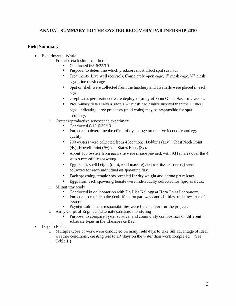
Since a new year class (YC) was

the objective for the Piney Point

2010 planting, the target area was

chosen because a large area of the

target shared a boundary with the

2007 and 2008 plantings, despite

much of the area having soft

return on the side scan.

The target area was surveyed with

the fish finder on the Paynter Lab boat prior to diver survey and only areas of hard return were surveyed

by divers, explaining the lack of diver coverage in the western portion of the target plot. The bottom

under transect 1 was deemed inappropriate for planting, due to the lack of exposed shell and the muddy

bottom. The bottom under transect 2 was determined to be good bottom for planting because of the

presence of exposed shell and hard bottom. At Piney Point, the diver survey found areas of hard bottom

on top of hard return from the side scan sonar.

Date Bar

Type Objective

Transect

#

#

Points

Mode

Exposed

Shell

Mode

Penetration

Mode

Substrate

5/13/10 MR New YC 1 100 Zero Knuckle Mud

5/13/10 MR New YC 2 50 Exposed Hard Bottom Loose shell

15

Since the objective

for the Strong Bay

2010 planting was

an overplanting, the

target area at Strong

Bay was chosen to

overlay both 2003

and 2007 plantings.

Although areas of

harder return were

found southeast of

the target, those

areas were not large

enough to

accommodate the 10

acre area needed for

GT.

The bottom under

both transect 1 and 2

were deemed appropriate for planting due to the presence of exposed shell and hard bottom in both

transects. Areas of dark side scan return were accompanied by hard bottom observations by divers at

Strong Bay.

Date Bar

Type Objective

Transect

#

#

Points

Mode

Exposed

Shell

Mode

Penetration

Mode

Substrate

6/11/10 S Overplant 1 100 Some Hard Bottom Loose Shell

6/11/10 S Overplant 2 100 Exposed Hard Bottom Loose Shell

16

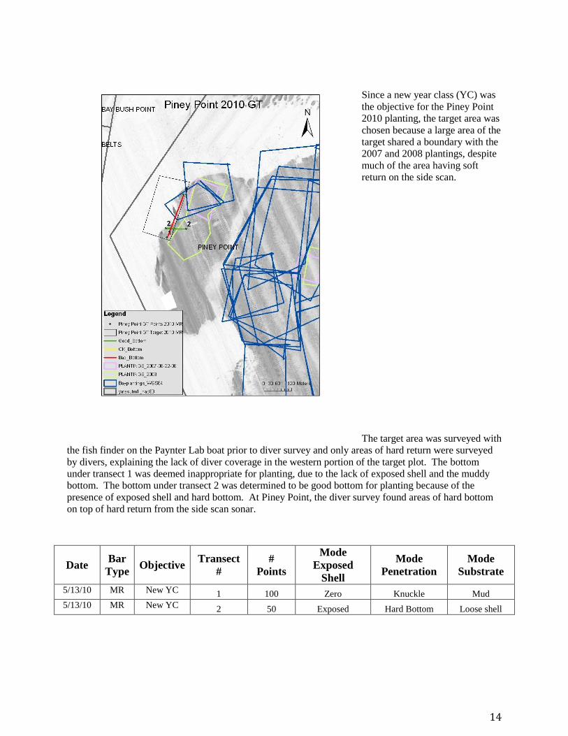
Since the objective for the

Blunt 2010 planting was 2

sites, both with new year

classes, the target areas were

chosen in between plantings

already on the bar. The

northern site was chosen due

to its proximity to other

plantings. The southern site

was chosen to explore a

previously bar-cleaned area

The bottom under the

transects in the northern

target area were deemed OK for planting because although no exposed shell was found, relatively low

penetration was observed on sandy bottom. Since this bar has been planted with success in the past,

future plantings on these areas could also be successful. Divers observed softer bottom than expected

when compared to the side scan return and Blunt. As expected, no oysters were observed on the bar-

cleaned site.

Date Bar

Type Objective

Transect

#

#

Points

Mode

Exposed

Shell

Mode

Penetration

Mode

Substrate

6/11/10 MR New YC 1 100 Zero Knuckle Sand




17

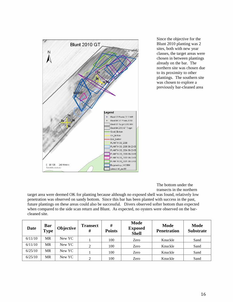
Since the objective

at Carpenter’s

Island was an

overplanting , a

target area was

chosen over an area

of hard side scan

return as well as a

planting that

occurred in 2006.

However, during the

diver survey, no

evidence of animals

from the 2006

planting was found.

The bottom under

both transect lines at

Carpenter’s Island were deemed appropriate for planting due the high amount of exposed shell present

covering the bottom. Areas of hard side scan return were accompanied by hard bottom observations by

divers at Carpenter’s Island.

Date Bar

Type Objective

Transect

#

#

Points

Mode

Exposed

Shell

Mode

Penetration

Mode

Substrate

6/25/10 MR Overplant 1 100 Exposed Knuckle Loose Shell

6/25/10 MR Overplant 2 100 Exposed Knuckle Loose Shell

18


Devil’s Playground 2010

planting was a new year class,

the target area was chosen in

an area of hard side scan

return that was flush with a

2005 planting and also still

within the boundaries of the

historical Yates bar. Since

the bottom within the target

area was only OK bottom,

another area outside of the

target was chosen for

confirmation of the side scan

return.

The bottom under transects 1

and 2 were deemed ok

bottom, due to the lack of exposed shell, amount of penetration and sandy bottom observed during the

survey. Transect 3 was conducted to confirm the hard return from the sonar was actually hard bottom.

The diver survey at Devil’s Playground confirmed the return from the side scan, with lighter return being

over OK bottom and darker return being over good bottom.

Date Bar

Type Objective

Transect

#

#

Points

Mode

Exposed

Shell

Mode

Penetration

Mode

Substrate



5/13/10 MR New YC 3 50 Exposed Hard Bottom Loose Shell

19


Hickory Thicket 2010 planting

was to overplant an existing

planting, the target area was

placed over the area of overlap

between the 2005 and 2007

plantings.

The transect taken at Hickory

Thicket indicated good bottom for planting due to presence of hard bottom and shell throughout the

transect. Only one transect was taken due to the overwhelming presence of good bottom that coincided

with hard side scan return. The side scan return at Hickory Thicket was confirmed by divers at this site.

Date Bar

Type Objective

Transect

#

#

Points

Mode

Exposed

Shell

Mode

Penetration

Mode

Substrate


20

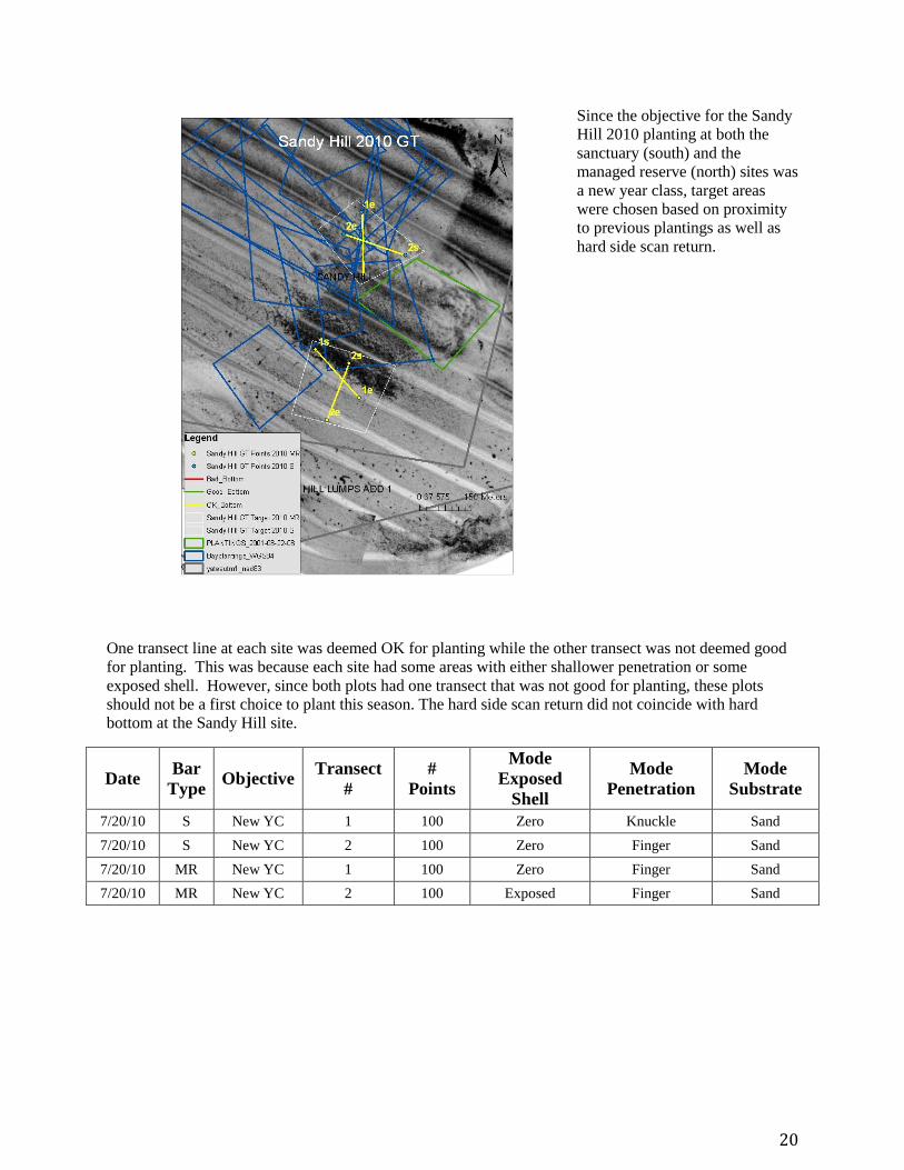
Since the objective for the Sandy

Hill 2010 planting at both the

sanctuary (south) and the

managed reserve (north) sites was

a new year class, target areas

were chosen based on proximity

to previous plantings as well as

hard side scan return.

One transect line at each site was deemed OK for planting while the other transect was not deemed good

for planting. This was because each site had some areas with either shallower penetration or some

exposed shell. However, since both plots had one transect that was not good for planting, these plots

should not be a first choice to plant this season. The hard side scan return did not coincide with hard

bottom at the Sandy Hill site.

Date Bar

Type Objective

Transect

#

#

Points

Mode

Exposed

Shell

Mode

Penetration

Mode

Substrate

7/20/10 S New YC 1 100 Zero Knuckle Sand

7/20/10 S New YC 2 100 Zero Finger Sand

7/20/10 MR New YC 1 100 Zero Finger Sand

7/20/10 MR New YC 2 100 Exposed Finger Sand

21

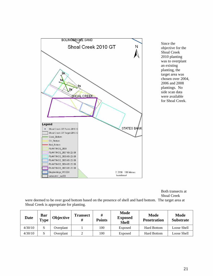
Since the

objective for the

Shoal Creek

2010 planting

was to overplant

an existing

planting, the

target area was

chosen over 2004,

2006 and 2008

plantings. No

side scan data

were available

for Shoal Creek.

Both transects at

Shoal Creek

were deemed to be over good bottom based on the presence of shell and hard bottom. The target area at

Shoal Creek is appropriate for planting.

Date Bar

Type Objective

Transect

#

#

Points

Mode

Exposed

Shell

Mode

Penetration

Mode

Substrate



22

Since the objective

for the States Bank

2010 planting was

to overplant an

existing planting,

the target area was

chosen over 2005,

2007 and 2008

plantings. The

target was also

placed next to a

large 2003 planting.

No side scan was

available for States

Bank.

Both transects at

States Bank were deemed to be over good bottom based on the presence of shell and hard bottom. The

target area at States Bank is appropriate for planting.

Date Bar

Type Objective

Transect

#

#

Points

Mode

Exposed

Shell

Mode

Penetration

Mode

Substrate


4/30/10 S Overplant 2 100 Exposed Knuckle Loose Shell

23

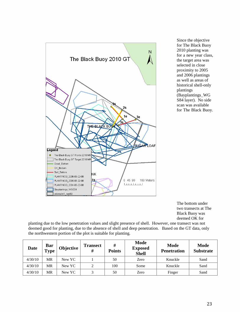
Since the objective

for The Black Buoy

2010 planting was

for a new year class,

the target area was

selected in close

proximity to 2005

and 2006 plantings

as well as areas of

historical shell-only

plantings

(Bayplantings_WG

S84 layer). No side

scan was available

for The Black Buoy.

The bottom under

two transects at The

Black Buoy was

deemed OK for

planting due to the low penetration values and slight presence of shell. However, one transect was not

deemed good for planting, due to the absence of shell and deep penetration. Based on the GT data, only

the northwestern portion of the plot is suitable for planting.

Date Bar

Type Objective

Transect

#

#

Points

Mode

Exposed

Shell

Mode

Penetration

Mode

Substrate


4/30/10 MR New YC 2 100 Some Knuckle Sand


24

Since the

objective for the

Bolingbroke

Sands 2010

planting was a

new year class,

the target area

was chosen to be

next to a high

concentration of

2006 plantings as

well as 2003 and

2008 plantings.

No side scan was

available for

Bolingbroke

Sands.

The bottom under

the transect lines at Bolingbroke Sands was not deemed appropriate for planting, due the lack of exposed

shell, relatively high penetration and sandy bottom.

Date Bar

Type Objective

Transect

#

#

Points

Mode

Exposed

Shell

Mode

Penetration

Mode

Substrate



25

Since the objective

for the Cooks

Point 2010

planting was a

new year class, the

target area was

placed over the

area of hardest

side scan return as

well as adjacent to

a historical shell-

only planting.

The bottom under

both transect lines

at Cooks Point

was deemed good for planting due to the presences of exposed shell and hard bottom. The diver survey

confirmed the hard return from the side scan sonar survey.

Date Bar

Type Objective

Transect

#

#

Points

Mode

Exposed

Shell

Mode

Penetration

Mode

Substrate

7/9/10 S New YC 1 100 Exposed Hard Bottom Sand

7/9/10 S New YC 2 100 Exposed Hard Bottom Loose Shell

26

Since the objective

for the Howell Point

2010 planting was a

new year class, the

target area was

chosen adjacent to

the 2001 planting

site and also on top

of a historical shell-

only planting. No

side scan was

available for the

target area at Howell

Point.

The bottom under

transect one was deemed bad for planting due to the absence of shell, relatively deep penetration and

sandy bottom. The bottom under transect two was better than that under transect one, with very little

exposed shell and less penetration than transect one, but sandy bottom was still observed under the second

transect.

Date Bar

Type Objective

Transect

#

#

Points

Mode

Exposed

Shell

Mode

Penetration

Mode

Substrate


7/9/10 MR New YC 2 100 Very Little Knuckle Sand

27


Mill Hill 2010 planting

was an overplanting, the

target area was chosen to

overlay 2002 and 2008

plantings as well as the

historical shell-only

plantings. The target area

was also chosen on an area

of hard side scan return.

The bottom under transect

one was deemed

unsuitable for a planting due to the absence of shell, the relatively deep penetration and the sandy bottom.

The bottom under transect two was slightly better than that under transect one, with some hard bottom,

but still zero shell and sandy substrate. Since transect two overlapped transect one, the bottom of transect

two may have been affected by the area under transect one. The hard side scan return observed at Mill

Hill was not confirmed by diver surveys of that area.

Date Bar

Type Objective

Transect

#

#

Points

Mode

Exposed

Shell

Mode

Penetration

Mode

Substrate

6/10/10 S Overplant 1 100 Zero Finger Sand

6/10/10 S Overplant 2 100 Zero Hard Bottom Sand

28

Since the objective for

the Tolly Point 2010

planting was an

overplanting, the target

area was selected to

overlap 1999, 2001 and

2006 plantings.

Although side scan was

available for the southern

portion of the bar,

previous diver surveys

had determined that area

to be unsuitable for

planting, so a northern

site was chosen.

The bottom under both

tracklines at Tolly Point

was deemed OK for planting, due to the low presence of shell on the bottom under transect one, the

relatively high penetration and the partially sandy bottom.

Date Bar

Type Objective

Transect

#

#

Points

Mode

Exposed

Shell

Mode

Penetration

Mode

Substrate

6/10/10 S Overplant 1 100 Some Knuckle Sand

6/10/10 S Overplant 2 100 Exposed Knuckle Loose Shell

29

Since the objective for the Duvall

2010 planting was to expand an

existing sanctuary, the target site

was chosen adjacent to a 1998 and a

2006 planting. No side scan data

was available for Duvall.

The bottom under all three transect

lines at Duvall was determined to be bad for planting due to the absence of shell and relatively high

penetration.

Date Bar

Type Objective

Transect

#

#

Points

Mode

Exposed

Shell

Mode

Penetration

Mode

Substrate

4/30/10 S Expansion 1 100 Zero Finger Sand



30

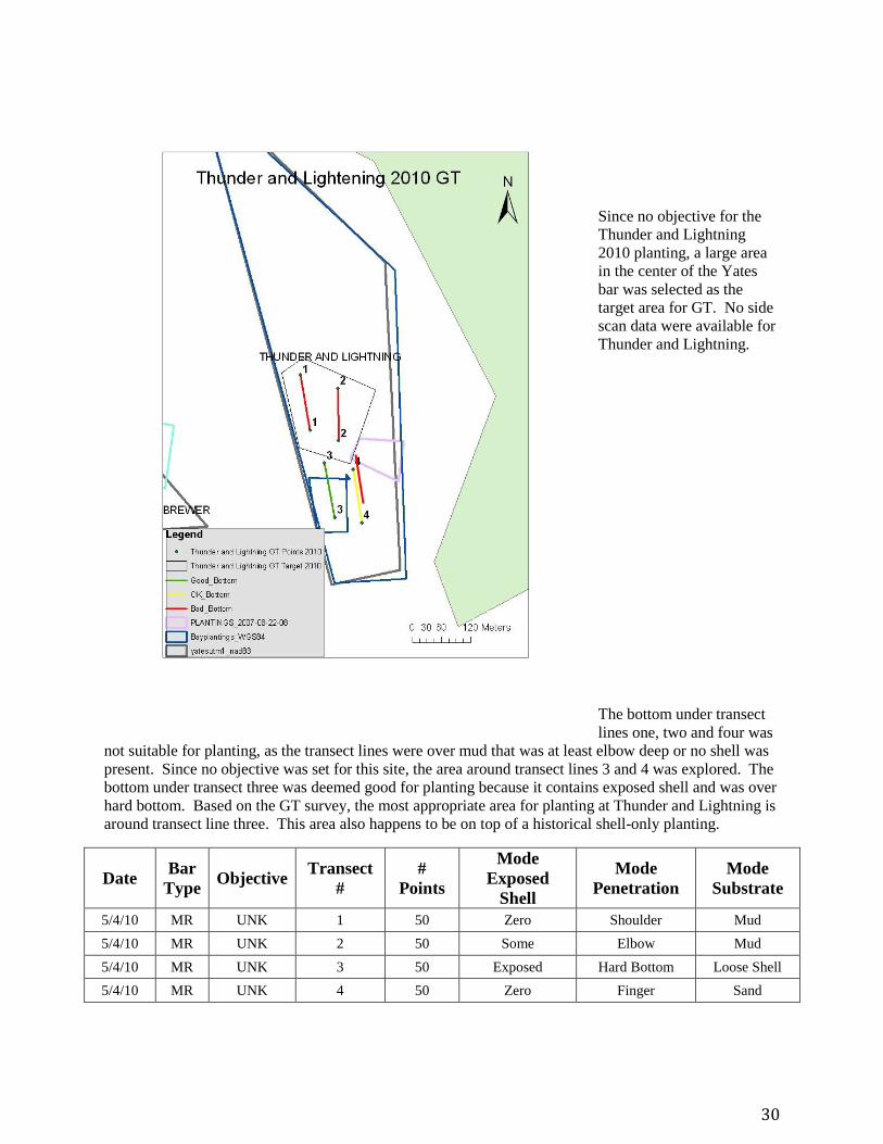
Since no objective for the

Thunder and Lightning

2010 planting, a large area

in the center of the Yates

bar was selected as the

target area for GT. No side

scan data were available for

Thunder and Lightning.

The bottom under transect

lines one, two and four was

not suitable for planting, as the transect lines were over mud that was at least elbow deep or no shell was

present. Since no objective was set for this site, the area around transect lines 3 and 4 was explored. The

bottom under transect three was deemed good for planting because it contains exposed shell and was over

hard bottom. Based on the GT survey, the most appropriate area for planting at Thunder and Lightning is

around transect line three. This area also happens to be on top of a historical shell-only planting.

Date Bar

Type Objective

Transect

#

#

Points

Mode

Exposed

Shell

Mode

Penetration

Mode

Substrate

5/4/10 MR UNK 1 50 Zero Shoulder Mud

5/4/10 MR UNK 2 50 Some Elbow Mud

5/4/10 MR UNK 3 50 Exposed Hard Bottom Loose Shell

5/4/10 MR UNK 4 50 Zero Finger Sand

31

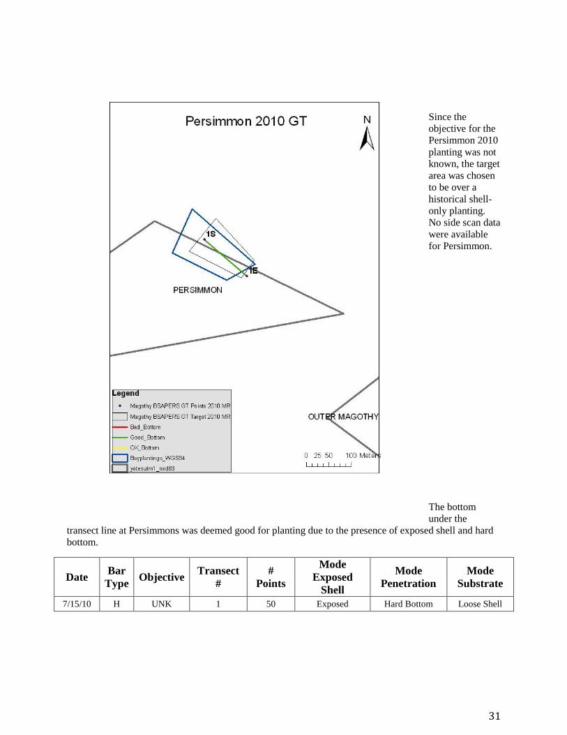
Since the

objective for the

Persimmon 2010

planting was not

known, the target

area was chosen

to be over a

historical shell-

only planting.

No side scan data

were available

for Persimmon.

The bottom

under the

transect line at Persimmons was deemed good for planting due to the presence of exposed shell and hard

bottom.

Date Bar

Type Objective

Transect

#

#

Points

Mode

Exposed

Shell

Mode

Penetration

Mode

Substrate

7/15/10 H UNK 1 50 Exposed Hard Bottom Loose Shell

32

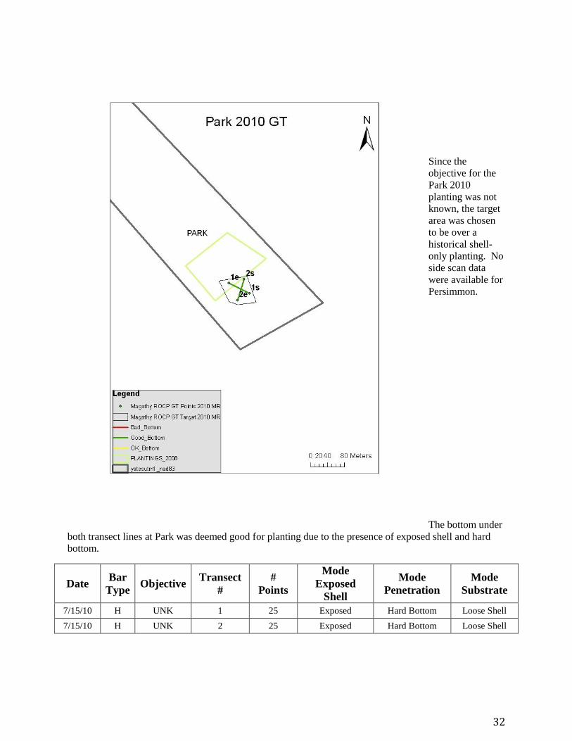
Since the

objective for the

Park 2010

planting was not

known, the target

area was chosen

to be over a

historical shell-

only planting. No

side scan data

were available for

Persimmon.

The bottom under

both transect lines at Park was deemed good for planting due to the presence of exposed shell and hard

bottom.

Date Bar

Type Objective

Transect

#

#

Points

Mode

Exposed

Shell

Mode

Penetration

Mode

Substrate



33

SECTION II Paynter Lab Post Planting Monitoring 2010


In 2010, 16 sites throughout Chesapeake Bay were surveyed by a diver 4-8 weeks after a planting of spat

on shell from the Horn Point Laboratory Oyster Hatchery in Cambridge, MD. The diver survey date,

number of acres planted, and the amount of spat planted at each of the 16 locations is presented in Table

1. As suggested by the planting dates, the 2010 plantings involved multiple plantings over the same areas.

Most sites were visited repeatedly and over-planted in an attempt to improve spat survival; this differs

from previous years that included a greater number of sites without over-planting.

Table 1 – 2010 post planting monitoring hatchery summary.

Site 2010 Planting

Dates

Sample

Date

Acres

Planted

Amount of Spat Planted

(millions) Blunt 6/21, 6/23, 6/28, 6/30 8/20/2010 6.46 34.41

Bolingbroke Sand 5/24 7/9/2010 10.52 6.94

Brewer 8/30, 9/1 10/21/2010 6.41 14.87

Cook Point 7/19, 7/26, 7/27, 8/2 9/21/2010 7.98 39.44

Hickory Thicket (East Neck

Bay) 7/5, 7/7, 7/12, 7/15 8/20/2010 7.06 32.04

Peach Orchard 8/23 10/21/2010 4.29 5.66

Sandy Hill (North) 7/21, 7/28, 8/4 8/26/2010 5.74 12.69

Sandy Hill (North)* 9/21 11/3/10 3.30 3.9

Sandy Hill (South)* 9/15, 10/4 11/3/10 4.79 3.9

Shoal Creek 5/12, 5/17, 5/18 7/9/2010 7.56 33.93

States Bank 5/5, 5/4, 5/10 7/9/2010 8.22 47.21

Strong Bay 6/7, 6/9, 6/14, 6/16 7/15/2010 8.85 45.95

Thunder and Lightning 9/13 10/21/2010 5.09 14.2

Wade 8/23 10/21/2010 2.36 5.33

Wade* 9/27 10/21/10 5.04 11.38

Weems Upper 8/3, 8/9, 8/11 10/21/2010 5.90 38.16

Using the planting boat’s track lines as a target, a diver collected hatchery shells from each survey

location. Divers placed a 0.3m x 0.3m quadrat on the bottom and collected all shells contained within the

quadrat. Attempts were made to collect six quadrat samples of varying shell densities (based on track

lines) at each site. When shell densities were too low for quadrat sampling, such that the diver could not

find shell in areas with few track lines, the diver would instead haphazardly collect 50 to 100 shells from

throughout the bar. Each shell was examined for live spat, boxes, scars, and gapers. Additionally, the

first fifty live spat observed in each sample were measured for shell height. The means of those shell

metrics are summarized in Table 2 for all sample locations in 2010.

34

Table 2 – 2010 post planting monitoring survey summary.

Average Count per Shell

Site River 2010 Planting Dates Survey

Date

# Shells

Sampled Live Gapers Scars Boxes

Shell

Height

(mm)

Blunt Chester 6/21, 6/23, 6/28, 6/30 8/20/2010 64 0.27 0.00 0.34 0.05 29.79

Bolingbroke Sand Choptank 5/24 7/9/2010 82 0.04 0.00 0.22 0.04 8.00

Brewer South 8/30, 9/1 10/21/2010 107 1.82 0.03 1.06 0.03 19.74

Cook Point Choptank 7/19, 7/26, 7/27, 8/2 9/21/2010 252 1.50 0.02 1.05 0.06 30.21

Hickory Thicket (East Neck

Bay) Chester 7/5, 7/7, 7/12, 7/15 8/20/2010 57 3.77 0.05 1.58 0.03 19.85

Peach Orchard Severn 8/23 10/21/2010 50 1.88 0.00 1.10 0.04 25.47

Sandy Hill (North) Choptank 7/21, 7/28, 8/4 8/26/2010 73 2.33 0.00 1.13 0.03 13.94

Sandy Hill (North) Choptank 9/21 11/3/2010 50 1.10 0.00 1.14 0.04 31.68

Sandy Hill (South) Choptank 9/15, 10/4 11/3/2010 101 1.26 0.00 1.31 0.36 7.70

Shoal Creek Choptank 5/12, 5/17, 5/18 7/9/2010 63 2.43 0.10 0.67 0.10 14.68

States Bank Choptank 5/5, 5/4, 5/10 7/9/2010 66 5.06 0.00 0.14 0.09 31.85

Strong Bay Chester 6/7, 6/9, 6/14, 6/16 7/15/2010 161 0.55 0.00 0.28 0.02 12.91

Thunder and Lightning South 9/13 10/21/2010 50 5.72 0.02 5.32 0.10 14.58

Wade Severn 8/23 10/21/2010 51 0.90 0.02 1.31 0.00 25.83

Wade Severn 9/27 10/21/2010 50 2.58 0.34 0.34 0.06 5.49

Weems Upper Severn 8/3, 8/9, 8/11 10/21/2010 50 1.26 0.02 0.46 0.00 30.31

In addition to the metrics listed above, each shell was inspected for the presence of Stylochus. Values are

not included in the table, as they were generally low across all sites. Stylochus were only observed at two

sites: Strong Bay in the Chester River (n=2) and the September Sandy Hill (North) planting in the

Choptank River (n=50).

35

The amount of spat per shell was multiplied by the total amount of shell planted on each bar to calculate the amount of spat detected by the post-

planting monitoring survey. Spat survival was then calculated as the percentage of spat planted that was detected by the survey. The mean spat

survival for 2010 plantings was 12.67% (±9.45). However, it is important to note the range of the data was 0.38% survival (Bolingbroke Sand) to

33.86% survival (Hickory Thicket). The percent survival of spat planted by bar is presented in Table 3. The 2008 and 2009 percent survival was

available for a small number of the bars monitored in 2010. The 2008 and 2009 percent survival were calculated from different data than

presented in Table 3 and are shown here to illustrate the large amount of annual variation in percent survival.

Table 3 – 2010 spat survival by bar.

Bar Name 2010 Planting

Dates

Acres

Planted

Mean #

Live

Spat/Shell

Amount of

Shell Planted

Amount of

Spat

Planted

(Millions)

Live Spat

Calculated from

Survey (Millions)

2010 %

Survival

2009 %

Survival

2008 %

Survival

Blunt 6/21, 6/23, 6/28,

6/30 6.46 0.27 2,880,000 34.41 0.78 2.3 4.4 -

Bolingbroke Sand 5/24 10.52 0.04 720,000 6.94 0.03 0.4 27.9 11.6

Brewer 8/30, 9/1 6.41 1.82 1,440,000 14.87 2.62 17.6 - -

Cook Point 7/19, 7/26, 7/27,

8/2 7.98 1.50 2,880,000 39.44 4.31 10.9 - -

Hickory Thicket (Big

Neck East)

7/5, 7/7, 7/12,

7/15 7.06 3.77 2,880,000 32.04 10.85 33.9 - -

Peach Orchard 8/23 4.29 1.88 360,000 5.66 0.68 12.0 - -

Sandy Hill (North) 7/21, 7/28, 8/4 6.29 2.33 960,000 12.69 2.24 17.6 - -

Sandy Hill (North) 9/21 5.50 1.10 640,000 12.88 0.70 5.5 - -

Sandy Hill (South) 9/15, 10/4 4.79 1.26 960,000 18.67 1.21 6.5 - -

Shoal Creek 5/12, 5/17, 5/18 7.56 2.43 2,160,000 33.93 5.25 15.5 12.8 44.6

States Bank 5/5, 5/4, 5/10 8.22 5.06 1,760,000 47.21 8.90 18.9 6.5 27.8

Strong Bay 6/7, 6/9, 6/14,

6/16 8.85 0.55 2,720,000 45.95 1.49 3.2 23.1 15.7

Thunder and Lightning 9/13 5.09 5.72 720,000 14.2 4.12 29.0 19.5 -

Wade 8/23 2.36 0.90 360,000 5.33 0.32 6.1 - -

Wade 9/27 5.04 2.58 720,000 11.38 1.86 16.3 - -

Weems Upper 8/3, 8/9, 8/11 5.90 1.26 2,160,000 38.16 2.72 7.1 - -

TOTAL/MEAN 373.76 48.07 12.7(±9.5) 15.7 24.9

36

Identical metrics were collected in 2008 and 2009 from sites comparable to those sampled in 2010 (see

Table 4). Fewer spat were planted in 2010 than 2009, and survival was fairly consistent. In 2008,

however, comparable amounts of total spat were planted relative to 2010, and survival in 2008 was higher,

although survival in all years was under 20%. In 2010, the total acreage planted was less than both 2008

and 2009, due to the fact that an over-planting approach was used where plantings were often repeated

over previous plantings.

Table 4 – Comparison of 2008, 2009, and 2010 summary survey metrics.

Means per Year

Sample

Year

Sample

Locations

Sites

Planted

Total

Acreage

Planted

Total

Spat

Planted

(Millions)

Initial

Spat per

Shell

Survey

Spat per

Shell

Shell

Height

(mm)

%

Survival SD

2008 20 27 215.64 369.95 30.23 3.94 14.94 17.0 14.4

2009 19 56 408.82 647.41 17.9 3.4 11.45 12.0 13.9

2010 13 16 323.44 373.76 14.86 2.03 20.13 12.8 9.5

In order to examine the source of the variability seen in post planting spat per shell and percent survival,

2008, 2009, and 2010 spat per shell and percent survival data were examined for relationships with

amount of spat and shell planted, density of spat and shell planted, spat growth rate, as well as location of

planting. In 2008 and 2010, no significant relationship was found between percent survival and any of

the variables examined, whereas 2009 data showed a negative relationship between initial spat per shell

and survival. It is possible that 2009 data was an anomaly, as 2008 and 2010 showed no such trend. The

2010 spat survival relative to initial spat per shell is shown below (Figure 1) and is also shown alongside

data from 2008 and 2009 (Figure 2). No trend was observed in survival relative to spat growth rate

(Figure 3), indicating that the environmental variation known to impact spat growth (oxygen

concentration, food availability) does not seem to be correlated with survival of spat in the northern

Chesapeake Bay. Additionally, 2010 data was evaluated for trends related to site salinity, timing of

planting, and whether or not the site was overplanted. These comparisons also yielded no obvious

relationships.

37

Figure 1–2010 data showing the spat survival as detected in post-planting monitoring surveys relative to

the initial hatchery spat planted. Data did not suggest a relationship between the two variables.

Figure 2–2008-2010 data showing the relationship between initial hatchery spat planted and spat survival,

as detected in post-planting monitoring surveys. No trend was observed across all three years, although

2009 data showed a distinct negative correlation between initial spat/shell and % survival.

0

5

10

15

20

25

30

35

40

0 5 10 15 20 25 30

% S

urv

ival

Initial Spat per Shell

2010 PPM Survival vs. Initial Spat per Shell

0

10

20

30

40

50

60

0 10 20 30 40 50 60

% S

urv

ival

Initial Spat per Shell

Annual Spat Survival Comparison

2010

2009

2008

38

Figure 3–No trend was observed in spat survival by spat growth rate (mm/day), indicating that the

environmental parameters known to impact spat growth (oxygen concentration, food availability) does

not seem to correlate with survival of spat in the northern Chesapeake Bay.

As mentioned above, in 2010 the sampling approach differed from previous years. Quadrat-based

sampling was used, per recommendations following the 2009 Paynter Lab report. The intent of quadrat

sampling in 2010 was to investigate the effects of shell density on survival. By using a quadrat to collect

shells within a standard area, density comparisons could be made. At each bar, divers attempted to

collect six total quads—three at a ―high density‖ area and three ―low density‖. High and low density sites

within a bar were selected based on the density of planting boat track lines at each bar.

At some sites, it was not possible to collect shells from a ―low density‖ area, and thus the quadrat-method

was not used. Below, Table 5 shows the bars sampled using quadrats, as well the metrics per quad.

(Data presented above in Table 2 for 2010 includes sums and averages of these quadrat data for

comparison across all bars.)

0.00

10.00

20.00

30.00

40.00

50.00

60.00

0.00 0.10 0.20 0.30 0.40 0.50 0.60 0.70

% S

urv

ival

Growth Rate (mm/day)

Effect of Growth Rate on Spat Survival

2010

2009

2008

39

Table 5–2010 post planting monitoring survey summary per quad.

Average per Shell

Site River Planting Dates Sample

Date

# of Shells

Sampled Live Gapers Scars Boxes

Shell Height

(mm)

Blunt Chester 6/21, 6/23, 6/28, 6/30 20-Aug-10 5 0.20 0.00 0.00 0.00 34.00



Blunt Chester 6/21, 6/23, 6/28, 6/30 20-Aug-10 11 0.00 0.00 0.36 0.27 -


Blunt Chester 6/21, 6/23, 6/28, 6/30 20-Aug-10 18 0.00 0.00 0.00 0.00 -

Brewer South 8/30, 9/1 21-Oct-10 8 1.63 0.00 0.63 0.00 20.23

Brewer South 8/30, 9/1 21-Oct-10 10 1.00 0.10 0.50 0.00 18.21

Brewer South 8/30, 9/1 21-Oct-10 13 2.92 0.08 0.69 0.00 18.23

Brewer South 8/30, 9/1 21-Oct-10 13 2.08 0.00 2.62 0.00 21.82

Brewer South 8/30, 9/1 21-Oct-10 17 1.29 0.00 0.82 0.12 20.04

Brewer South 8/30, 9/1 21-Oct-10 46 1.98 0.00 1.09 0.07 19.90

Cook Point Choptank 7/19, 7/26, 7/27, 8/2 21-Sep-10 2 1.00 0.00 0.00 0.00 30.00






Hickory Thicket Chester 7/5, 7/7, 7/12, 7/15 20-Aug-10 7 4.57 0.00 0.57 0.00 23.37






Sandy Hill (North) Choptank 7/21, 7/28, 8/4 26-Aug-10 6 3.33 0.00 1.67 0.00 13.95






Sandy Hill (South) Choptank 9/15, 10/4 03-Nov-10 7 0.14 0.00 1.86 0.14 9.00






States Bank Choptank 5/5, 5/4, 5/10 09-Jul-10 1 6.00 0.00 0.00 0.00 33.33






Strong Bay Chester 6/7, 6/9, 6/14, 6/16 15-Jul-10 2 2.00 0.00 0.00 0.00 19.25






40

The amount of live spat per shell in each quad was multiplied by the total amount of shell found in each

quad to calculate the amount of spat per quad detected by the post-planting monitoring survey. Spat

survival was then calculated as the percentage of spat planted (per quad as the initial spat per shell

multiplied by the total shells per quad) that was detected by the survey. The mean per quad spat survival

for 2010 plantings was 12.37%. However, it is important to note the range of the data was 0.00% survival

(Blunt and Strong Bay) to 43.29% survival (States Bank). As in the complete 2010 data, quad-based

survival data shows high variability. The percent survival of spat planted by bar is presented in Table 6.

41

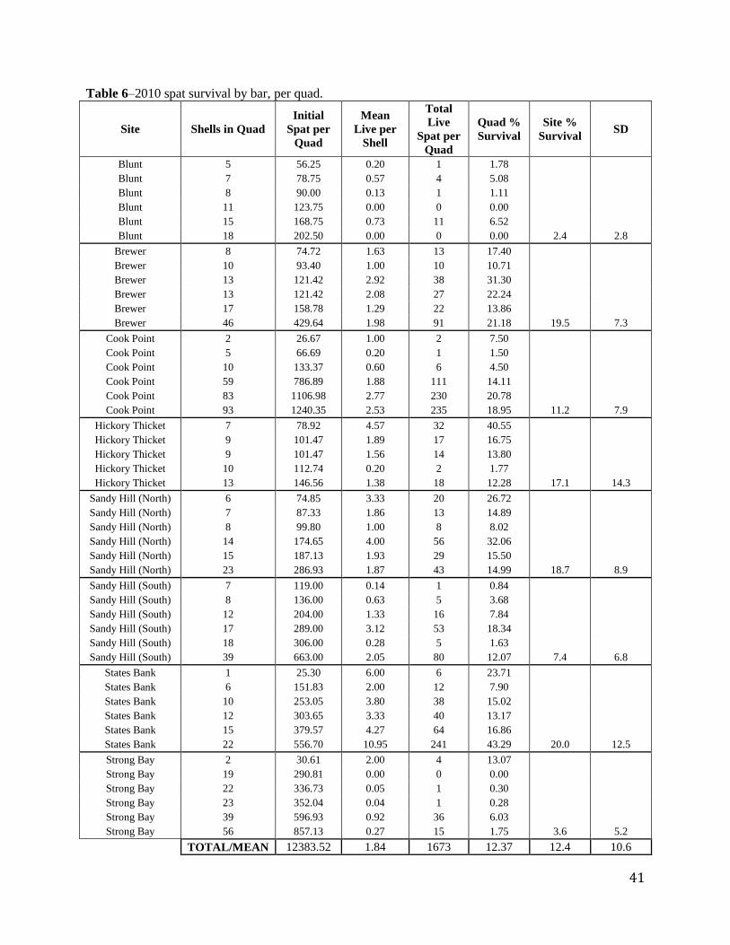
Table 6–2010 spat survival by bar, per quad.

Site Shells in Quad

Initial

Spat per

Quad

Mean

Live per

Shell

Total

Live

Spat per

Quad

Quad %

Survival

Site %

Survival SD

Blunt 5 56.25 0.20 1 1.78

Blunt 7 78.75 0.57 4 5.08

Blunt 8 90.00 0.13 1 1.11

Blunt 11 123.75 0.00 0 0.00

Blunt 15 168.75 0.73 11 6.52

Blunt 18 202.50 0.00 0 0.00 2.4 2.8

Brewer 8 74.72 1.63 13 17.40

Brewer 10 93.40 1.00 10 10.71

Brewer 13 121.42 2.92 38 31.30

Brewer 13 121.42 2.08 27 22.24

Brewer 17 158.78 1.29 22 13.86

Brewer 46 429.64 1.98 91 21.18 19.5 7.3

Cook Point 2 26.67 1.00 2 7.50

Cook Point 5 66.69 0.20 1 1.50

Cook Point 10 133.37 0.60 6 4.50

Cook Point 59 786.89 1.88 111 14.11

Cook Point 83 1106.98 2.77 230 20.78

Cook Point 93 1240.35 2.53 235 18.95 11.2 7.9

Hickory Thicket 7 78.92 4.57 32 40.55

Hickory Thicket 9 101.47 1.89 17 16.75

Hickory Thicket 9 101.47 1.56 14 13.80

Hickory Thicket 10 112.74 0.20 2 1.77

Hickory Thicket 13 146.56 1.38 18 12.28 17.1 14.3

Sandy Hill (North) 6 74.85 3.33 20 26.72

Sandy Hill (North) 7 87.33 1.86 13 14.89

Sandy Hill (North) 8 99.80 1.00 8 8.02

Sandy Hill (North) 14 174.65 4.00 56 32.06

Sandy Hill (North) 15 187.13 1.93 29 15.50

Sandy Hill (North) 23 286.93 1.87 43 14.99 18.7 8.9

Sandy Hill (South) 7 119.00 0.14 1 0.84

Sandy Hill (South) 8 136.00 0.63 5 3.68

Sandy Hill (South) 12 204.00 1.33 16 7.84

Sandy Hill (South) 17 289.00 3.12 53 18.34

Sandy Hill (South) 18 306.00 0.28 5 1.63

Sandy Hill (South) 39 663.00 2.05 80 12.07 7.4 6.8

States Bank 1 25.30 6.00 6 23.71

States Bank 6 151.83 2.00 12 7.90

States Bank 10 253.05 3.80 38 15.02

States Bank 12 303.65 3.33 40 13.17

States Bank 15 379.57 4.27 64 16.86

States Bank 22 556.70 10.95 241 43.29 20.0 12.5

Strong Bay 2 30.61 2.00 4 13.07

Strong Bay 19 290.81 0.00 0 0.00

Strong Bay 22 336.73 0.05 1 0.30

Strong Bay 23 352.04 0.04 1 0.28

Strong Bay 39 596.93 0.92 36 6.03

Strong Bay 56 857.13 0.27 15 1.75 3.6 5.2

TOTAL/MEAN 12383.52 1.84 1673 12.37 12.4 10.6

42

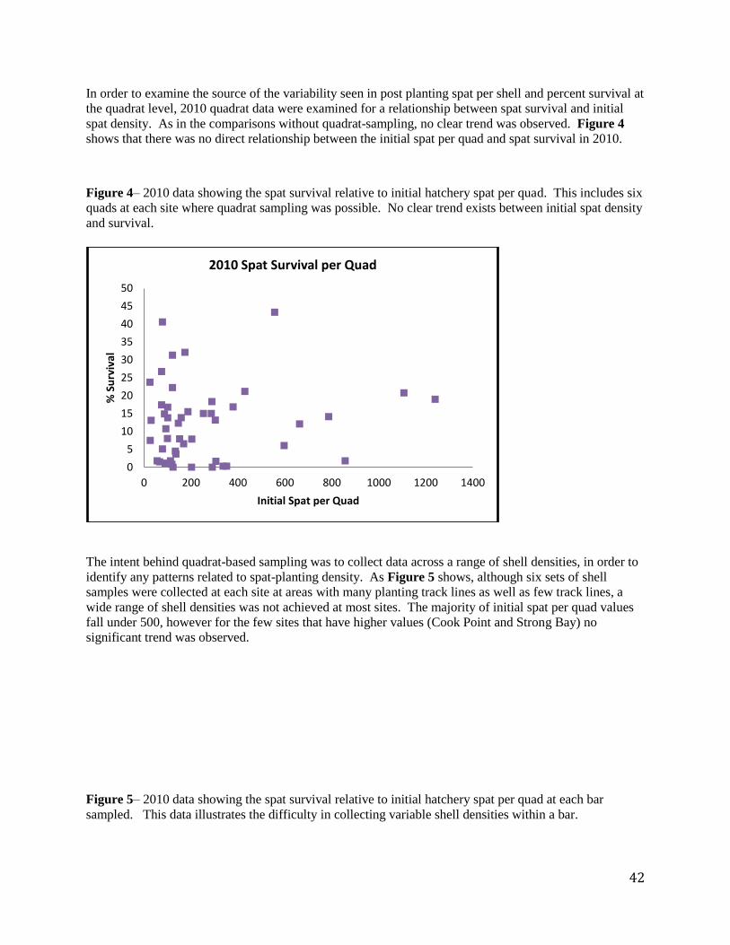
In order to examine the source of the variability seen in post planting spat per shell and percent survival at

the quadrat level, 2010 quadrat data were examined for a relationship between spat survival and initial

spat density. As in the comparisons without quadrat-sampling, no clear trend was observed. Figure 4

shows that there was no direct relationship between the initial spat per quad and spat survival in 2010.

Figure 4– 2010 data showing the spat survival relative to initial hatchery spat per quad. This includes six

quads at each site where quadrat sampling was possible. No clear trend exists between initial spat density

and survival.

The intent behind quadrat-based sampling was to collect data across a range of shell densities, in order to

identify any patterns related to spat-planting density. As Figure 5 shows, although six sets of shell

samples were collected at each site at areas with many planting track lines as well as few track lines, a

wide range of shell densities was not achieved at most sites. The majority of initial spat per quad values

fall under 500, however for the few sites that have higher values (Cook Point and Strong Bay) no

significant trend was observed.

Figure 5– 2010 data showing the spat survival relative to initial hatchery spat per quad at each bar

sampled. This data illustrates the difficulty in collecting variable shell densities within a bar.

0

5

10

15

20

25

30

35

40

45

50

0 200 400 600 800 1000 1200 1400

% S

urv

ival

Initial Spat per Quad

2010 Spat Survival per Quad

43

Conclusions:

The 2010 planting season involved several changes attempting to achieve greater survival success and

more relevant data. First, the planting approach differed from previous years, as fewer bars were planted

overall, but were over-planted over multiple trips to each bar. Additionally, while not a highly

controllable factor, the number of initial spat per shell was lower in 2010 than previous years. Neither of

these differences appears to have had a drastic impact on spat survival, as the overall 2010 spat survival

was consistent with that of 2009.

Using the data collected in post-planting monitoring surveys, the relationship between initial spat per

shell and spat survival were compared, yielding no significant trend for 2010. This is similar to data from

2008, however 2009 data showed a negative correlation between initial spat per shell and survival.

Continued post-planting monitoring surveys in 2011 could help identify the relationship seen in 2009 as

an anomaly or possible trend.

In an effort to more closely examine the relationship between initial spat planted and post-planting

survival, surveys were conducted using a standard sample area (a 0.3m x 0.3m quadrat). This allowed for

a stronger comparison of initial spat density over a specific area. Using this approach, 2010 data again

showed no relationship among initial spat density and post-planting spat survival. As mentioned above,

although a range of shell density sample sets were targeted, this was not achieved at most sites. It is

recommended that quadrat-based sampling is continued in 2011 surveys, possibly with greater focus on

high-density areas within bars to create the desired density range. This can also be enhanced through

continued over-planting as was done in 2010.

0

5

10

15

20

25

30

35

40

45

50

0 200 400 600 800 1000 1200 1400

% S

urv

ival

Initial Spat per Quad

2010 Spat Survival per Quad at Each Site

Blunt

Brewer

Cook Point

Hickory Thicket

Sandy Hill

Sandy Hill 2

States Bank

Strong Bay

45

SECTION III Paynter Lab Patent Tong Survey 2010


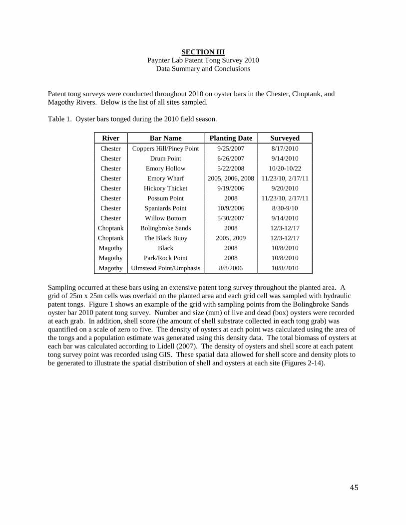
Patent tong surveys were conducted throughout 2010 on oyster bars in the Chester, Choptank, and

Magothy Rivers. Below is the list of all sites sampled.

Table 1. Oyster bars tonged during the 2010 field season.

River Bar Name Planting Date Surveyed

Chester Coppers Hill/Piney Point 9/25/2007 8/17/2010

Chester Drum Point 6/26/2007 9/14/2010

Chester Emory Hollow 5/22/2008 10/20-10/22

Chester Emory Wharf 2005, 2006, 2008 11/23/10, 2/17/11

Chester Hickory Thicket 9/19/2006 9/20/2010

Chester Possum Point 2008 11/23/10, 2/17/11

Chester Spaniards Point 10/9/2006 8/30-9/10

Chester Willow Bottom 5/30/2007 9/14/2010

Choptank Bolingbroke Sands 2008 12/3-12/17

Choptank The Black Buoy 2005, 2009 12/3-12/17

Magothy Black 2008 10/8/2010

Magothy Park/Rock Point 2008 10/8/2010

Magothy Ulmstead Point/Umphasis 8/8/2006 10/8/2010

Sampling occurred at these bars using an extensive patent tong survey throughout the planted area. A

grid of 25m x 25m cells was overlaid on the planted area and each grid cell was sampled with hydraulic

patent tongs. Figure 1 shows an example of the grid with sampling points from the Bolingbroke Sands

oyster bar 2010 patent tong survey. Number and size (mm) of live and dead (box) oysters were recorded

at each grab. In addition, shell score (the amount of shell substrate collected in each tong grab) was

quantified on a scale of zero to five. The density of oysters at each point was calculated using the area of

the tongs and a population estimate was generated using this density data. The total biomass of oysters at

each bar was calculated according to Lidell (2007). The density of oysters and shell score at each patent

tong survey point was recorded using GIS. These spatial data allowed for shell score and density plots to

be generated to illustrate the spatial distribution of shell and oysters at each site (Figures 2-14).

46

Figure 1. Example of a patent tong grid used in the 2010 patent tong season. Each grid cell is 25x25m in

size and each black point represents one patent tong grab.

Table 2 summarizes the metrics collected for each site sampled in 2010 (amount of live and dead oysters,

percentage of oysters found that were dead, live oyster size and density, percent of area sampled with

greater than 5oy/m2, percent of area sampled with shell coverage, population estimate, total biomass and

Perkinsus marinus (Dermo) prevalence and weighted prevalence). At The Black Buoy and Emory Wharf,

multiple year classes were sampled and disease was determined separately for each age class. For both

sites, older animals had higher disease prevalence and weighted prevalence than their younger

counterparts.

47

Table 2. Data collected on 2010 patent tong surveys.

Bar Name Year

Planted

# Live Oysters

Collected

# Dead Oysters

Collected

Dead

Oysters

(% of Total)

Average

Live

Oyster Length

SD

Average

Live Oyster

Density

(#/m2)

SD % Total

Area

>5oy/m2

% Total

Area with

Shell Coverage

Population Estimate

(Oysters)

Biomass

(kg)

Dermo Prevalence

(%)

Dermo Weighted

Prevalence

Coppers Hill/Piney Point 2007 626 19 3 95 19 9 18 57 99 216,160 290 20.0 0.17

Drum Point 2007 73 2 3 107 24 1 2 4 35 25,207 46 10.0 0.01

Emory Hollow 2008 2244 36 2 87 17 14 20 73 89 631,561 862 3.3 0.03

Hickory Thicket 2006 346 29 8 84 19 2 4 8 87 119,475 124 12.0 0.04

Spaniards Point 2006 1036 42 4 109 16 2 3 4 70 357,735 665 80.0 1.05

Willow Bottom 2007 28 0 0 110 17 0 1 1 36 9,669 18 58.6 0.26

Bolingbroke Sands 2006 400 32 7 92 21 2 4 7 52 155,280 232 100.0 1.73

The Black Buoy 2005 667 37 5 65 40 3 10 20 60 258,929 162 33.3 0.14

The Black Buoy 2009 - - - - - - - - - - - 7.4 0.003

Black 2008 114 4 3 74 14 1 9 4 1 39,365 30 6.7 0.10

Park/Rock Point 2008 67 5 7 75 16 2 5 4 13 23,135 18 10.7 0.04

Ulmstead Point/Umphasis 2006 518 10 2 98 15 15 25 69 80 178,867 261 20.0 0.21

Emory Wharf 2008 201 17 8 113 26 7 5 11 49 69,406 138 83.3 0.65

Emory Wharf 2005, 2006

- - - - - - - - - - - 26.7 0.27

Possum Point 2005,

2006 171 8 5 119 17 26 4 62 70 59,047 142 30.0 0.14

2010 Mean - 499 19 4 95 - 6 - 25 57 - - 33.5 0.32

2010 Total - - - - - - - - - - 2,143,835 2,988 - -

48

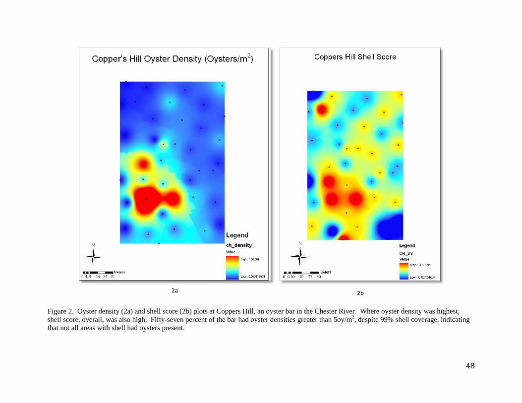
Figure 2. Oyster density (2a) and shell score (2b) plots at Coppers Hill, an oyster bar in the Chester River. Where oyster density was highest,

shell score, overall, was also high. Fifty-seven percent of the bar had oyster densities greater than 5oy/m2, despite 99% shell coverage, indicating

that not all areas with shell had oysters present.

2a 2b

49

Figure 3. Oyster density (3a) and shell score (3b) plots at Drum Point, an oyster bar in the Chester River. Where oyster density was highest, shell

score, overall, was also high. However, oyster densities and shell coverage were low at this bar; only 4% of the bar contained oysters at densities

higher than 5oy/m2 and only 35% of the bar had any shell coverage.

3a 3b

50

Figure 4. Oyster density (4a) and shell score (4b) plots at Emory Hollow, an oyster bar in the Chester River. Generally, shell score was higher in

areas of high oyster density and 73% of the bar had oyster densities greater than 5oy/m2. However, oysters were not found in all areas with shell,

as 89% of the bar had shell coverage.

4a 4b

51

Figure 5. Oyster density (5a) and shell score (5b) plots at Hickory Thicket, an oyster bar in the Chester River. Shell scores were higher in the

center of the bar where most oysters were found, but only 8% of the bar had oyster densities greater than 5oy/m2, while 87% of the bar had shell

coverage.

5a 5b

52

Figure 6. Oyster density (6a) and shell score (6b) plots at Spaniard’s Point, an oyster bar in the Chester River. Overall, in areas of high oyster

density, shell score was also high. However, only 4% of the bar had oyster densities greater than 5oy/m2 while 70% of the bar had shell coverage,

indicating that not all areas with shell had oysters present.

6a 6b

53

Figure 7. Oyster density (7a) and shell score (7b) plots at Willow Bottom, an oyster bar in the Chester River. Although the one area of high oyster

density did occur on an area with high shell score, this bar’s oyster and shell coverage are both poor overall. Only 1% of the bar has oyster density

greater than 5oy/m2 and only 36% of the bar had any shell coverage.

7b 7a

54

Figure 8. Oyster density (8a) and shell score (8b) plots at Bolingbroke Sands an oyster bar in the Choptank River. Areas of high oyster density

also had high shell scores, however not all areas of high shell score yielded high oyster density. However, only 7% of the bar had oyster densities

greater than 5oy/m2, while 52% of the bar had shell coverage, indicating that not all areas with shell had oysters present.

8a 8b

55

Figure 9. Oyster density (9a) and shell score (9b) plots at The Black Buoy, an oyster bar in the Choptank River. Areas of highest oyster density

did not occur in areas of highest shell score, however some shell coverage was present where all oysters were found. Twenty percent of the bar

had oyster densities greater than 5oy/m2 and 60% of the bar had shell coverage, indicating that not all areas with shell had oysters present.

9a 9b

56

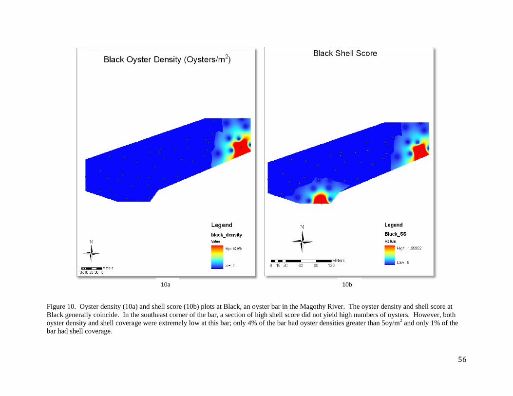
Figure 10. Oyster density (10a) and shell score (10b) plots at Black, an oyster bar in the Magothy River. The oyster density and shell score at

Black generally coincide. In the southeast corner of the bar, a section of high shell score did not yield high numbers of oysters. However, both

oyster density and shell coverage were extremely low at this bar; only 4% of the bar had oyster densities greater than 5oy/m2 and only 1% of the

bar had shell coverage.

10a 10b

57

Figure 11. Oyster density (11a) and shell score (11b) plots at Park, an oyster bar in the Magothy River. In general, the two areas of high oyster

density (on the east edge of the bar and the center of the northern edge) were also areas of high shell score. However, multiple areas of high shell

score did not yield high oyster density. Both oyster density and shell coverage were extremely low at this bar; only 4% of the bar had oyster

densities greater than 5oy/m2 and only 13% of the bar had shell coverage.

11a 11b

58

Figure 12. Oyster density (12a) and shell score (12b) plots at Ulmstead Point, an oyster bar in the Magothy River. Areas of high oyster density

also had high shell scores, however not all high shell scores yielded high oyster densities. Sixty-nine percent of the bar had oyster densities greater

than 5oy/m2 and 80% of the bar had shell coverage, indicating that not all areas with shell had oysters present.

12a 12b

59

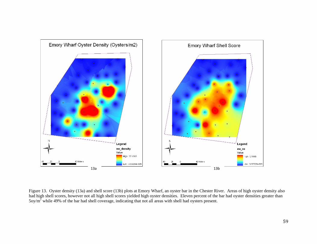
Figure 13. Oyster density (13a) and shell score (13b) plots at Emory Wharf, an oyster bar in the Chester River. Areas of high oyster density also

had high shell scores, however not all high shell scores yielded high oyster densities. Eleven percent of the bar had oyster densities greater than

5oy/m2 while 49% of the bar had shell coverage, indicating that not all areas with shell had oysters present.

13a 13b

60

Figure 14. Oyster density (14a) and shell score (14b) plots at Possum Point, an oyster bar in the Chester River. Areas of high oyster density also

had high shell scores, however not all high shell scores yielded high oyster densities. Shell score and oyster densities greater than 5 oysters/m2

were similar in amount and location at this bar, with 62% of the bar having oyster densities greater than 5 oysters/m2 and 70% of the bar having

shell coverage. However, the small size of this bar (2.1 acres) may influence the high continuity of these measurements.

14a 14b

61

Conclusions:

Overall, oyster density and shell score appear to be related in that, in areas of high oyster density shell

score was also high. A majority of the plots, however, show that areas of high shell score did not yield

high oyster density. This suggests that high shell score is not always associated with the presence of live

oysters, although areas with high oyster density tend to also have high shell coverage. Unsurprisingly,

bars with high populations also had high oyster biomass. Mean oyster density in 2010 was 5oy/m2, but

only 23% of the area surveyed achieved greater than that density. Fifty-seven percent of the area

surveyed had any shell coverage, again indicating that shell coverage is greater than oyster coverage on

the bars sampled. Considering that just over 50% of the area surveyed had any shell, we suggest that

future patent tong sampling be limited to areas where shell has been found in the past. This will reduced

the area necessary to sample by about half, allowing for a greater number of bars to be sampled in the

future. A more quantitative method of determining the amount of shell on each bar will be developed in

2011 to more accurately estimate shell coverage. Although an extensive restoration program has been

undertaken by the ORP, it is clear that restored bars do not have complete shell or oyster coverage,

indicating that higher density restoration efforts are necessary to create more successfully restored habitat

and therefore more successful oyster populations.

Additionally, long term patent tong data was evaluated from Coppers Hill, Drum Point, Willow Bottom,

and Ulmstead Point. These four bars have been monitored annually since 2007 and the data for these

sites is available in Section IV.

63

SECTION IV Paynter Lab Intensive Oyster Bar Long-Term Patent Tong Monitoring

2007-2010

In order to obtain a temporally sound representation of oyster population dynamics over time following a

spat on shell planting, four individual oyster bars were monitored for four consecutive years (2007-2010).

These bars, their location, harvest status and planting dates are outlined in Table 1 below.

Table 1. Oyster bars targeted for long-term monitoring.

Bar Name Location Harvest Status Planting Dates Coppers Hill Chester River Managed Reserve 9/25/07, 4/28/08

Drum Point Chester River Managed Reserve 6/26/2007

Ulmstead Point Magothy River Sanctuary 8/8/2006

Willow Bottom Chester River Managed Reserve 5/30/2007

Sampling occurred at these bars using an extensive patent tong survey throughout the planted area. A

grid of 25m x 25m cells was overlaid on the planted area and each grid cell was sampled with hydraulic

patent tongs. Number and shell height (mm) of live and dead (box) oysters were recorded at each grab.

The density of oysters at each point was calculated using the area of the tongs and a population estimate

was generated using this density data. The biomass of oysters found at each site was calculated using the

following equation: Biomass(g) =0.00003*( Shell Height(mm)^2.3512) (Liddel 2007). This equation

was used to calculate the total biomass in each surveyed cell; cell data was then totaled to determine each

bar’s biomass. The density of oysters at each patent tong survey point was recorded using GIS in 2008-

2010. These spatial data allowed for a density plot to be generated for each year to illustrate the spatial

distribution of oysters at each site for 2008-2010. Results for individual sites are presented below.

Coppers Hill Coppers Hill is a managed reserve bar located in the Chester River that was planted in both 2007 and

2008. However, the patent tong survey for 2007 was conducted before the planting occurred. The size

distribution of oysters sampled at Coppers Hill indicated a small number of adult oysters in 2007, high

numbers of spat in 2008 followed by a decline in the amount of spat but an increase in their size in 2009,

with an amplification of that pattern in 2010 (Fig. 1). The biomass of oysters at Coppers Hill was also

reflective of the planting and growth activities at the bar from 2007-2010 (Fig. 2). The low biomass in

2007 reflected the low number of oysters surveyed; however, 2007 oysters were larger than the spat

surveyed in 2008, also indicated by the fairly small increase in biomass in 2008. 2008 oysters were many,

but small, as the bar was planted after the survey in 2007 and again in 2008. Together, figures 1 and 2

show that a high abundance of oysters did not necessarily entail high biomass. Data from 2009 showed a

very slight increase in biomass, which could be reflective of high spat mortality after the 2008 planting.

In 2010, as oyster size increased biomass also grew. The total biomass for each year was consistent with

the size distribution of oysters in each year, indicating the patent tong survey detected the size distribution

and relative amounts of oysters on Coppers Hill before and after planting.

64

Figure 1. Size frequency of oysters sampled at Coppers Hill during 2007-2010 patent tong surveys.

Coppers Hill was planted in 2007 (after patent tong survey) and 2008. The size frequencies indicate the

patent tong survey detected the size distribution and relative amounts of oysters on Coppers Hill before

and after planting.

Figure 2. Biomass of oysters at Coppers Hill during 2007-2010 patent tong surveys. The biomass of

oysters at Coppers Hill was consistent with the size distribution of oysters in each year.

The survey statistics for Coppers Hill are presented in Table 2 below. Similar to the trends observed in

the size frequency distribution and total biomass data, the increase in live count and decline in mean shell

height from 2007 to 2008 was indicative of the 2008 planting. Since the patent tong survey for 2007 was

conducted before the 2007 planting, the low live count and relatively high mortality (as box count % of

live) was not unexpected for the large, older population that was sampled. The oyster density, population

estimates and biomass estimates follow a similar pattern, with 2007 having lower mean density,

population and biomass than both 2008 and 2009. The 2009 patent tong survey showed an increase in

mean shell height paired with declines in live count, mortality, mean density and population. The 2010

survey indicated a small increase in live count, mortality, mean density, population and biomass. We

0

50

100

150

200

250

300

350Fr

eq

ue

ncy

Shell Height (mm)

2007

2008

2009

2010

0

50

100

150

200

250

300

350

2007 2008 2009 2010

Coppers Hill Annual Biomass (kg)

65

believe these increases are reflective of the natural variability present in the system as it reaches a

sustainable post-planting population.

Table 2. Patent tong survey statistics for Coppers Hill.

Sampling

Year

Mean Shell

Height (mm)

Live

Count

Box

Count

Box Count

(% of Total)

Mean Density

(oysters/m2)

Population

Abundance

Biomass

Sum (kg)

2007 102 86 28 25 1 29,696 48

2008 51 803 57 7 13 277,279 93

2009 77 462 8 2 7 159,530 128

2010 94 626 19 3 9 216,160 290

The density plots for Coppers Hill are presented in Figure 2 below. Oyster density in 2008 reached as

high as 125 oysters/m2, mostly concentrated in the middle and eastern portion of the planting; however a

majority of the site had no oysters present (Fig. 2a). In contrast, in 2009 oyster density reached a

maximum of 62 oysters/m2, mostly concentrated in the southern half of the planting (Fig. 2b). This

decline in density and shift in the location of oysters was indicative of activity that occurred on this bar

between the 2008 and 2009 patent tong surveys. The 2010 survey found oysters in the same general

location as the 2009 survey, but at slightly higher densities (106 oysters/m2).

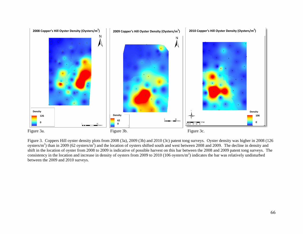
66

Figure 3a. Figure 3b. Figure 3c.

Figure 3. Coppers Hill oyster density plots from 2008 (3a), 2009 (3b) and 2010 (3c) patent tong surveys. Oyster density was higher in 2008 (126

oysters/m2) than in 2009 (62 oysters/m

2) and the location of oysters shifted south and west between 2008 and 2009. The decline in density and

shift in the location of oyster from 2008 to 2009 is indicative of possible harvest on this bar between the 2008 and 2009 patent tong surveys. The

consistency in the location and increase in density of oysters from 2009 to 2010 (106 oysters/m2) indicates the bar was relatively undisturbed

between the 2009 and 2010 surveys.

2010 Copper’s Hill Oyster Density (Oysters/m2) 2009 Copper’s Hill Oyster Density (Oysters/m

2) 2008 Copper’s Hill Oyster Density (Oysters/m

2)

126 0

62 0

106 0

Density

Density

Density

Density

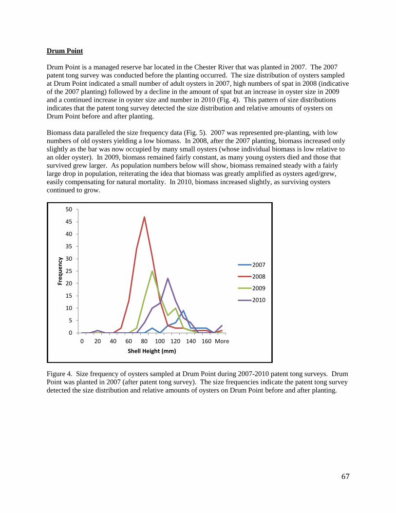
67

Drum Point

Drum Point is a managed reserve bar located in the Chester River that was planted in 2007. The 2007

patent tong survey was conducted before the planting occurred. The size distribution of oysters sampled

at Drum Point indicated a small number of adult oysters in 2007, high numbers of spat in 2008 (indicative

of the 2007 planting) followed by a decline in the amount of spat but an increase in oyster size in 2009

and a continued increase in oyster size and number in 2010 (Fig. 4). This pattern of size distributions

indicates that the patent tong survey detected the size distribution and relative amounts of oysters on

Drum Point before and after planting.

Biomass data paralleled the size frequency data (Fig. 5). 2007 was represented pre-planting, with low

numbers of old oysters yielding a low biomass. In 2008, after the 2007 planting, biomass increased only

slightly as the bar was now occupied by many small oysters (whose individual biomass is low relative to

an older oyster). In 2009, biomass remained fairly constant, as many young oysters died and those that

survived grew larger. As population numbers below will show, biomass remained steady with a fairly

large drop in population, reiterating the idea that biomass was greatly amplified as oysters aged/grew,

easily compensating for natural mortality. In 2010, biomass increased slightly, as surviving oysters

continued to grow.

Figure 4. Size frequency of oysters sampled at Drum Point during 2007-2010 patent tong surveys. Drum

Point was planted in 2007 (after patent tong survey). The size frequencies indicate the patent tong survey

detected the size distribution and relative amounts of oysters on Drum Point before and after planting.

0

5

10

15

20

25

30

35

40

45

50

0 20 40 60 80 100 120 140 160 More

Fre

qu

en

cy

Shell Height (mm)

2007

2008

2009

2010

68

Figure 5. Biomass of oysters at Drum Point during 2007-2010 patent tong surveys. The biomass of

oysters at Drum Point was consistent with the size distribution of oysters in each year.

The survey statistics for Drum Point are presented in Table 3 below. Similar to the trends in the size

frequency distribution and biomass data, the increase in live count and decline in mean shell height from

2007 to 2008 was indicative of the 2008 planting. Since the patent tong survey for 2007 was conducted

before the 2007 planting, the low live count and relatively high mortality (as box count % of live) is not

unexpected for the large, older population that was sampled. The oyster density and population estimates

follow a similar pattern, with 2007 having lower mean density and population than both 2008 and 2009.

The 2009 patent tong survey shows an increase in mean shell height paired with decline in live count,

mortality, mean density and population. The 2010 survey indicated an increase in live count, mortality,

mean density and population. Total biomass remained steady despite a fairly large drop in population,

underscoring that biomass was greatly amplified as oysters aged/grew, easily compensating for natural

mortality. We believe these increases are reflective of the natural variability present in the system as it

reaches a sustainable post-planting population.

Table 3. Patent tong survey statistics for Drum Point.

Sampling

Year

Mean Shell

Height (mm)

Live

Count

Box

Count

Box Count

(% of Live)

Mean Density

(oysters/m2)

Population

Abundance

Biomass Sum

(kg)

2007 123 13 8 38 <1 4,316 11

2008 80 97 7 7 1 33,494 28

2009 92 26 2 7 <1 8,978 32

2010 107 73 2 3 1 25,207 46

The density plots for Drum Point are presented in Figure 6 below. Oyster density in 2008 reached 12

oysters/m2, mostly concentrated in the north and eastern portion of the planting (Fig. 6a). In contrast, in

2009 oyster density reached a maximum of 6 oysters/m2, spread throughout the planting (Fig. 6b). This

decline in density and shift in the location of oyster is indicative of activity that occurred on this bar

between the 2008 and 2009 patent tong surveys. The 2010 survey indicated another shift in the location

of oysters on Drum Point, although at such low maximum densities (9 oysters/m2), the patent tong survey

could have missed other areas of relative high density on the bar.

0

10

20

30

40

50

2007 2008 2009 2010

Drum Point Annual Biomass (kg)

69


Figure 6. Drum Point oyster density plots from 2008 (6a), 2009 (6b) and 2010 (6c) patent tong surveys. Oyster density was higher in 2008 (12

oysters/m2) than in 2009 (6 oysters/m

2) and the location of oysters shifted between 2008 and 2009. The decline in density and shift in the location

of oyster from 2008 to 2009 is indicative of possible harvest on this bar between the 2008 and 2009 patent tong surveys. Maximum oyster density

remained low in 2010 (9 oysters/m2) and although the density plot indicates a shift in the location of oysters, the low density of oysters at the bar

make it difficult for the patent tongs to accurately capture all areas of relative high density on the bar.

2010 Drum Point Oyster Density (Oysters/m2) 2009 Drum Point Oyster Density (Oysters/m

2) 2008 Drum Point Oyster Density (Oysters/m

2)

6 0

9 0

12 0

Density

Density Density

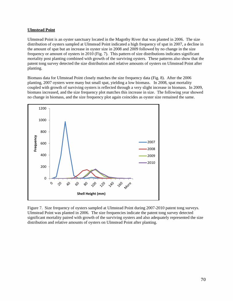
70

Ulmstead Point

Ulmstead Point is an oyster sanctuary located in the Magothy River that was planted in 2006. The size

distribution of oysters sampled at Ulmstead Point indicated a high frequency of spat in 2007, a decline in

the amount of spat but an increase in oyster size in 2008 and 2009 followed by no change in the size

frequency or amount of oysters in 2010 (Fig. 7). This pattern of size distributions indicates significant

mortality post planting combined with growth of the surviving oysters. These patterns also show that the

patent tong survey detected the size distribution and relative amounts of oysters on Ulmstead Point after

planting.

Biomass data for Ulmstead Point closely matches the size frequency data (Fig. 8). After the 2006

planting, 2007 oysters were many but small spat, yielding a low biomass. In 2008, spat mortality

coupled with growth of surviving oysters is reflected through a very slight increase in biomass. In 2009,

biomass increased, and the size frequency plot matches this increase in size. The following year showed

no change in biomass, and the size frequency plot again coincides as oyster size remained the same.

Figure 7. Size frequency of oysters sampled at Ulmstead Point during 2007-2010 patent tong surveys.

Ulmstead Point was planted in 2006. The size frequencies indicate the patent tong survey detected

significant mortality paired with growth of the surviving oysters and also adequately represented the size

distribution and relative amounts of oysters on Ulmstead Point after planting.

0

200

400

600

800

1000

1200

Fre

qu

en

cy

Shell Height (mm)

2007

2008

2009

2010

71

Figure 8. Biomass of oysters at Ulmstead Point during 2007-2010 patent tong surveys. The biomass of

oysters at Ulmstead Point is consistent with the size distribution of oysters in each year.

The survey statistics for Ulmstead Point are presented in Table 4 below. Similar to the trends in the size

frequency distribution, the highest live count and smallest shell heights were observed in 2007, a decline

in live count and an increase in mean shell height in 2008, an unexpected increase in live count and mean

shell height in 2009 with oyster size and population leveling off in 2010. High spat mortality (as box

count % of live) was observed in the first year post planting and dramatically declined in the following

years post planting. The oyster density and population estimates follow a similar pattern, with 2007

having higher mean density and population than 2008-2010. The 2008 patent tong survey showed a

decline in live count, mortality, mean density, population and biomass, however, the 2009 survey

indicated an increase in these metrics from the year before. The 2010 survey data indicated that the

population is leveling off in the fourth year post-planting to contain a steady density, population and

biomass of animals.

Table 4. Patent tong survey statistics for Ulmstead Point.

Sampling

Year

Mean Shell

Height (mm)

Live

Count

Box

Count

Box Count

(% of Live)

Mean Density

(oysters/m2)

Population

Abundance

Biomass

Sum (kg)

2007 27 625 161 20 20 225,138 19

2008 75 281 19 6 10 96,858 75

2009 94 512 1 0.2 19 176,796 228

2010 98 518 10 2 15 178, 867 261

The density plots for Ulmstead Point are presented in Figure 9 below. Oyster density in 2008 reached 50

oysters/m2, spread throughout the planting (Fig. 9a). In 2009 oyster density reached a maximum of 80

oysters/m2, also spread throughout the planting (Fig. 9b). Finally, 2010 oyster density reached a

maximum of 94 oysters/m2 consistently spread throughout the planting. The consistency in the density

and spatial distribution of oysters on this sanctuary may be evidence of the undisturbed nature of this bar.

0

50

100

150

200

250

300

2007 2008 2009 2010

Ulmstead Point Annual Biomass (kg)

72


Figure 9. Ulmstead Point oyster density plots from 2008 (9a), 2009 (9b) and 2010 (9c) patent tong surveys. Oyster density and location remained

consistent between 2008-2010, with density increasing slightly from year to year: 2008 (50 oysters/m2), 2009 (oysters/m

2), and 2010 (94

oysters/m2). The consistency in density and location of oyster from 2008 through 2010 may be indicative of the undisturbed nature of this bar.

2010 Ulmstead Point Density (Oysters/m2) 2009 Ulmstead Point Oyster Density (Oysters/m

2) 2008 Ulmstead Point Oyster Density (Oysters/m

2)

50 0

81 0

94 0

Density

Density Density

73

Willow Bottom

Willow Bottom is a managed reserve bar located in the Chester River that was planted in 2007. The

patent tong survey for 2007 was conducted before the planting occurred and no oysters were found in that

survey. The size distribution of oysters sampled at Willow Bottom indicated consistency in the number

of oysters sampled in 2008 and 2009 paired with a shift to larger oysters from 2008 to 2009, with the

2010 size distribution data indicating a decline in the number of oysters but an increase in surviving

animals’ shell heights (Fig. 7). This pattern of size distributions indicates high survival from year two to

year three post-planting and also points to significant growth between years.

Biomass data at Willow Bottom complements the size frequency data. Figure 11 showed no biomass for

2007, as no oysters were found. 2008’s high number of spat after the 2007 planting had much lower

biomass than in 2009, indicating the large oyster growth that occurred between 2008 and 2009. In 2010,

oyster growth was coupled with some mortality, and biomass remained constant, although population

abundance decreased (Table 5).

Figure 10. Size frequency of oysters sampled at Willow Bottom during 2007-2010 patent tong surveys.

Willow Bottom was planted in 2007 after the patent tong survey and no oysters were found during the

survey that year. The size frequencies indicate high survival from year two to year three post-planting

and significant growth between all years at Willow Bottom.

0

2

4

6

8

10

12

14

16

18

Fre

qu

en

cy

Shell Heights (mm)

2008

2008

2010

2009

74

Figure 11. Biomass of oysters at Willow Bottom during 2007-2010 patent tong surveys. The biomass of

oysters at Willow Bottom is consistent with the size distribution of oysters in each year.

The survey statistics for Willow Bottom are presented in Table 5 below. The highest live count and

population was observed in 2009, with an unexpected decline in live count and population in 2010. Low

spat mortality (as box count % of live) was observed when oysters were found at the site. Although the

size frequency distributions indicated some mortality between 2009 and 2010, no dead oysters were found

in the 2010 survey, indicating that oysters were either more spread out throughout the bar in 2010 or the

survey did not capture the amount of dead oysters on the bar accurately. However, the low live counts

and populations observed at Willow Bottom during the entire survey period may prevent the patent tong

from accurately capturing oyster densities. Total biomass increased from 2008 to 2009, indicating that

growth outpaced death between these two years. Biomass remained fairly consistent from 2009 to 2010,

showing that the existing population may be stabilizing 3 years after planting.

Table 5. Patent tong survey statistics for Willow Bottom.

Sampling

Year

Mean Shell

Height (mm)

Live

Count

Box

Count

Box Count

(% of Live)

Mean Density

(oysters/m2)

Population

Abundance

Biomass

Sum (kg)

2007 N/A 0 0 N/A 0 0 0

2008 74 16 0 0 <1 5,352 8

2009 87 47 1 2 <1 16,229 18

2010 110 28 0 0 <1 9,668 18

The density plots for Willow Bottom are presented in Figure 12 below. Maximum oyster density was low

in all years (4 oysters/m2 in 2008, 8 oysters/m

2 in 2009, and 9 oysters/m

2 in 2010). Spatially, oysters were

spread throughout the planting in 2008 and concentrated to the eastern half in 2009 and 2010. The

increase in density and the shift in spatial distribution of oysters from 2008 to 2009 may be indicative of

activity on this bar in the period between the two surveys.

0.00

5.00

10.00

15.00

20.00

2007 2008 2009 2010

Willow Bottom Annual Biomass (kg)

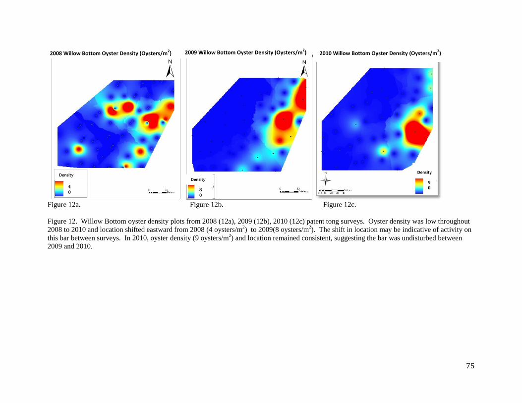
75


Figure 12. Willow Bottom oyster density plots from 2008 (12a), 2009 (12b), 2010 (12c) patent tong surveys. Oyster density was low throughout

2008 to 2010 and location shifted eastward from 2008 (4 oysters/m2) to 2009(8 oysters/m

2). The shift in location may be indicative of activity on

this bar between surveys. In 2010, oyster density (9 oysters/m2) and location remained consistent, suggesting the bar was undisturbed between

2009 and 2010.

2010 Willow Bottom Oyster Density (Oysters/m2) 2009 Willow Bottom Oyster Density (Oysters/m

2) 2008 Willow Bottom Oyster Density (Oysters/m

2)

4 0

8 0

9 0

Density Density

Density

76

Conclusions

The long term patent tong data for these four sites indicate that patent tongs are appropriately

characterizing the addition, growth and distribution of oysters on managed reserves and sanctuaries. The

frequency distributions of shell height reflected the addition of oysters by a shift in the mean size and

number of oysters present. The frequency distributions also reflected the growth of oysters post-planting,

through a drop in numbers of oysters paired with an increase in mean shell height. Although a large

amount of variability exists in the population estimates, the bars sampled generally declined after the first

year of sampling post-planting and then remained relatively consistent in the years following (see Figure

13 below).

Figure 13. Oyster population at each bar sampled by sampling year. Although a large amount of variability exists in

the population estimates, the bars sampled generally declined after the first year of sampling post-planting and then

remained relatively consistent in the years following.

Biomass data show an increase in biomass over time at each bar and complemented the size frequency

data, emphasizing at all four bars the influence that oyster size has on biomass relative to population size

(see Figure 14 below). At each bar, changes in population abundance might have been offset by

increasing biomass, as surviving oysters continued to grow. The summary statistics and population

estimates accurately reflected the activities occurring on bars between sampling events, whether a

planting occurred or the bar remained unchanged. The density plots were able to display not only the

changes in the density of oysters between years, but also in their distribution. These shifts in distribution

and density may be a tool for managers to use to detect illegal activity on oyster bars. On bars that

remained unchanged post-planting, survey data indicate a leveling-off of oyster density and distribution

three to four years post planting.

0

50,000

100,000

150,000

200,000

250,000

300,000

2007 2008 2009 2010

Oy

ste

r P

op

ula

tio

n

Sampling Year

Total Estimated Oyster Population 2007-2010

Coppers Hill

Drum Point

Ulmstead Point

Willow Bottom

77

Figure 14. Total oyster biomass (in kg) at each bar sampled by sampling year. Biomass increased at each bar

through time, despite a drop in average oyster size, emphasizing the influence that oyster size has on biomass at each

bar sampled.

On oyster bars with low oyster densities (i.e. less than 10 oysters/m2), and thus low populations, the

distribution of animals was patchy and therefore changes in the population estimates and spatial

distribution of animals was heavily influenced by one or two patent tong samples. Although these data

are generally capturing the nature of undisturbed oyster bars to equalize their oyster densities, populations,

and spatial distributions over time post-planting, it is important to survey small bars such as these at the

fine scales currently being sampled by the Paynter Lab in order to accurately portray oyster population

dynamics on these bars.

References

Liddel, M.K. ―A von Bertalanffy Model for the Estimation of Oyster (Crassostrea virginica) Growth on

Restored Oyster Reefs in the Chesapeake Bay‖. Ph.D. dissertation, University of Maryland, College Park,

2007

0

50

100

150

200

250

300

350

2007 2008 2009 2010

To

tal

Bio

ma

ss (

kg

)

Sampling Year

Total Oyster Biomass 2007-2010

Coppers Hill

Drum Point

Ulmstead Point

Willow Bottom

79

SECTION V

Paynter Lab Lessons Learned 2010

Ground Truthing

In general, areas of hard side scan return were confirmed to be hard bottom by divers. This result

underscores the importance of having side scan data available prior to conducting GT surveys, as it makes

the survey more efficient. 2010 was the first year in which side scan data were available for many GT

sites and our results indicate that this process should continue into the future. The cooperation of MGS

and NCBO was critical in this endeavor, and their participation was much appreciated. Our GT data

provided confirmation of existing bottom conditions and these data are currently being analyzed with the

help of MGS to understand the precision of the side scan sonar in determining bottom type. We hope to

continue this analysis into the future. Our goal should be to confidently use side scan sonar to predict

bottom quality without the need for diver confirmation.

Perkinsus marinus Infection

Mean Perkinsus marinus (Dermo) prevalence and intensity were low in 2010, and not significantly

different from values reported for 2008 and 2009. These findings indicated that dermo was not a large

factor in oyster mortality in the northern Chesapeake Bay, although sub-lethal infection rates may play a

role in declines in the ecosystem services provided by those infected oysters, such as a decline in

fecundity or filtration rates. A few exceptions existed at Spaniards Point (a weighted prevalence of 1.23),

in the Chester River and Bolingbroke Sands (a weighted prevalence of 1.3), in the Choptank River. These

populations should be exhaustively harvested.

80

Post Planting Monitoring

Conclusions:

The 2010 planting season involved several changes in an attempt to achieve greater survival success and

more relevant data. First, the planting approach differed from previous years, as fewer bars were planted

overall, but were over-planted by multiple trips to each bar. Additionally, while not a highly controllable

factor, the number of initial spat per shell was lower in 2010 than previous years. Neither of these

differences appeared to have had a drastic impact on spat survival, as the overall 2010 spat survival was

consistent with 2008 and 2009.

Using the data collected in post-planting monitoring surveys, the relationship between initial spat per

shell and spat survival were compared, yielding no significant trend for 2010. This was similar to data

from 2008, however 2009 data showed a negative correlation between initial spat per shell and survival.

Additional post-planting monitoring surveys in 2011 could help identify the relationship seen in 2009 as

an anomaly or possible trend.

In an effort to more closely examine the relationship between initial spat planted and post-planting

survival, surveys were conducted using a standard sample area (a 1m2 quadrat). This allowed for a

stronger comparison of initial spat density over a specific area. Using this approach, 2010 data again

showed no relationship among initial spat density and post-planting spat survival. As mentioned above,

although a range of shell density sample sets were targeted, this was not achieved at most sites. It is

recommended that quadrat-based sampling is continued in 2011 surveys, possibly with greater focus on

high-density areas within bars to create the desired density range. This can also be enhanced through

continued over-planting as was done in 2010.

Recommendations:

Identifying the factors influencing spat survival in the Chesapeake Bay is critical to the restoration of

oysters in Maryland. Students and staff of the Paynter Lab have identified four main factors thought to

influence spat survival: environmental variation, spat density, predation and spat size upon planting.

Although environmental variation may have a large impact on spat survival, our lab would like to focus

on factors whose impact could be reduced by manipulating current restoration techniques.

81

Spat Density

The density of spat on a given planting may affect spat survival. We propose to examine the effect of

spat density on survival at both the experimental and bar-levels.

Bar-Level Density Experiment:

In 2010, the effect of spat density on survival was examined opportunistically on planted bars throughout

the Chesapeake Bay (see 2010 PPM report for results). At each bar, divers attempted to collect six total

quads—three at a ―high density‖ area and three ―low density‖. High and low density sites within a bar

were selected based on the density of planting boat track lines at each bar. Although the data from this

preliminary experiment indicate that spat density does not impact spat survival, we would like to repeat

this experiment in 2011 to confirm these results. Quads will be used to collect spat at six locations on

each planting in 2011 to continue to explore the relationship between spat density and survival at the bar

level.

Experimental-Level Density Experiment:

A main complication of the bar-level experiment was the lack of range of densities of spat that occurred

post planting (0-100 spat/m2). Considering this lack of density range, we would also like to conduct a

density experiment in which spat densities are manipulated at a small scale. In August of 2011, spat on

shell will be obtained from the Horn Point Laboratory oyster hatchery in Cambridge, Maryland. The

initial number and size of spat on shell will be provided by the hatchery. Shells will be placed in 1m2

quadrats deployed on the shell bed at densities of 50, 100, 200 and 400 shells per square meter on Glebe

Bay oyster bar in the South River. Three replicates of each density will be deployed, totaling 12 quadrats

on the bottom. One quadrat of each density will be kept in a flow-through tank at the Horn Point

Laboratory oyster hatchery to serve as controls. Quadrats will be left on the bottom for 4-8 weeks, at

which time the shells will be collected and spat on shell number and size will be measured and compared

between densities. Below is a schematic of one replicate (of three) of the experimental design.

4.2m

3m

50

100

200

Screw Anchor

400

82

Predation

Many predators of spat exist in the Chesapeake Bay, but the direct affects of predation on spat survival in

Maryland are not well understood. In 2010, an experiment was conducted in an attempt to quantify the

affects of predation on spat survival. 1m3 cages were lined with either ¼ inch screening, 1/8 inch

screening, window screening or were left open to exclude large predators, small predators, worms and no

predators, respectively. About 20 shells with varying numbers of spat on shell were placed inside each

cage and cages were deployed in Glebe Bay for 2 weeks in June of 2010. 20 shells were placed in the

live well of the Paynter Lab boat as a control. Data from this first deployment was not analyzed due to

many confounding factors in the experimental deployment and design. Primarily, the deployment and

retrieval of the cages caused significant tearing the ¼ inch mesh, eliminating the smallest mesh size from

the design. Also, no predators were captured upon retrieval of the cages, limiting the ability to determine

the type and number of predators in each treatment. Finally, mud crabs were found in the live well when

shells were removed, eliminating the control from the experiment. We propose to conduct a more

streamlined experiment in 2011 (see below).

Spat on shell will be obtained from the Horn Point Laboratory oyster hatchery after a one to two week

nursery period. This will allow for the identification of spat on shell with the naked eye and consistency

in the number of spat in each cage upon deployment. In order to confirm the absence of a cage effect,

three cages and three open cages will be deployed on the target bar (Green Marsh oyster bar in the

Choptank River) for one full field day. In addition, a control will be maintained at the Horn Point

Laboratory oyster hatchery using flow-through water from the Choptank River. Three treatments will be

created out of 1m2 cages: open cage (total predation exposure), ¼ inch screening compartment (small

predator exposure) and 1 mm aluminum mesh window screening compartment (worm predation

exposure). Each treatment will be replicated four times, for a total of 12 cages. Cages will be loaded

with a consistent number and density of shells and spat (15-25 shells with 70-100 spat per cage). Cages

will be designed to allow for the predators inside each cage to be captured when cages are retrieved. To

account for the need to secure spat to the cage frame in the ―open‖ treatment, all shells will be attached to

each cage by monofilament wire and glue. A sub-sample of shells will be kept at the hatchery to serve as

a control. Cages will be deployed during July 2011 for two weeks. Spat size and number as well as

predator abundance and diversity will be determined in each cage and compared to initial and control data.

Below is a schematic of the cage design and experimental deployment (one of four replicates).

Spat Size

Window Screen

Open Cage 3m

6m

Screw Anchor

¼” Screen

Open Cage

83

Spat Size

In 2009, a spat survival experiment was performed at Sandy Hill oyster Bar in the Choptank River, which

showed that spat survival (as measured by number of spat per shell and spat shell height) was independent

of planting size and substrate type. However, this experiment had several confounding factors and we

would like to perform a similar study in a more complete fashion. Three separate plantings of both

hatchery and nursery spat on shell should be conducted within two weeks of each other, again at Sandy

Hill or a bar in close proximity, in June of 2011. In order to understand the effects of spat size on survival

over time, we would like to measure spat number and size according to the following schedule:

Day # Spat Type Time Amount of Shell Collected

1 Hatchery

Before shell is loaded onto planting boat 50 from hatchery tank

Nursery 50 from nursery tank

1 Hatchery

Before planting 50 from planting boat Nursery

1 Hatchery

1 hr post-planting 50 from planted area Nursery

2-7 Hatchery

Any 50 from planted area Nursery

14 Hatchery


45 Hatchery


We believe that the data provided by the previous three experiments will allow for a greater

understanding of the factors affecting spat survival in the Chesapeake Bay and will provide guidelines for

more efficient restoration in the future.

84

Patent Tonging

Overall, oyster density and shell score appear to be related in that, in areas of high oyster density shell

score was also high. A majority of the plots, however, showed that areas of high shell score did not yield

high oyster density. This suggested that high shell score was not always associated with the presence of

live oysters, although areas with high oyster density tended to also have high shell coverage.

Unsurprisingly, bars with high populations also had high oyster biomass. Mean oyster density in 2010

was 5oy/m2, but only 23% of the area surveyed achieved greater than that density. Fifty-seven percent of

the area surveyed had any shell coverage, again indicating that shell coverage is greater than oyster

coverage on the bars sampled. Considering that just over 50% of the area surveyed had any shell, we

suggest that future patent tong sampling be limited to areas where shell has been found in the past. This

will reduced the area necessary to sample by about half, allowing for a greater number of bars to be

sampled in the future. A more quantitative method of determining the amount of shell on each bar will be

developed in 2011 to more accurately estimate shell coverage. Although an extensive restoration

program has been undertaken by the ORP, it is clear that restored bars do not have complete shell or

oyster coverage, indicating that higher density restoration efforts are necessary to create more

successfully restored habitat and therefore more successful oyster populations.

The long term patent tong data for these four sites indicated that patent tongs were appropriately

characterizing the addition, growth and distribution of oysters on managed reserves and sanctuaries. The

frequency distributions of shell height reflected the addition of oysters by a shift in the mean size and

number of oysters present. The frequency distributions also reflected the growth of oysters post-planting,

through a drop in numbers of oysters paired with an increase in mean shell height. Biomass data

complemented the size frequency data, emphasizing at all four bars the influence that oyster size had on

biomass relative to population size. At each bar, drops in population abundance were offset by an

increase in biomass, as surviving oysters continued to grow. The summary statistics and population

estimates accurately reflected the activities occurring on bars between sampling events, whether a

planting occurred or the bar remained unchanged. The density plots were able to display not only the

changes in the density of oysters between years, but also in their distribution. These shifts in distribution

and density may be a tool for managers to use to detect illegal activity on oyster bars. On bars that

remained unchanged post-planting, survey data indicated a leveling-off of oyster density and distribution

three to four years post planting.

On oyster bars with low oyster densities (and therefore populations) the distribution of animals was

patchy and therefore changes in the population estimates and spatial distribution of animals was heavily

influenced by one or two patent tong samples. Although these data were generally capturing the nature of

undisturbed oyster bars to equalize their oyster densities, populations, and spatial distributions over time

post-planting, it was important to survey small bars such as these at the fine scale currently being sampled

by the Paynter Lab in order to accurately portray oyster population dynamics on these bars.

85

Overall Summary

Due to the complexities of the Chesapeake Bay ecosystem, successful restoration requires the hard work

and collaboration of many people and agencies. The oyster restoration program in Maryland relies on

accurate data on the location, density and health of Maryland oysters to make informed management

decisions. The successful collaboration of the Paynter Lab, the Maryland Geological Survey and

NOAA’s Chesapeake Bay Office to synthesize existing side scan sonar images with data on the true

topography of the bay (as collected by diver observation) is the first step in the restoration process. This

synthesis will not only make the determination of future restoration sites more efficient, it will also allow

for quantification of the available bottom for future restoration efforts in Maryland.

Understanding the population dynamics of the existing oyster populations in Maryland is the next step in

making informed restoration decisions in the future. Systematic patent tong surveys of managed reserve

and sanctuary bars in 2010 have revealed low oyster densities across most bars, with only 23% of bar

acreage having densities over 5oy/m2. Shell coverage was better than oyster coverage across bars, with

57% of the area surveyed by patent tongs having shell coverage. However, this percentage only seems

high compared to the low amount of oyster coverage on restored bars in Maryland. In order to achieve

self-sustaining oyster populations through restoration efforts, the amount of shell coverage and oyster

densities must be increased.

Another obstacle to the success of restoration is post-planting spat mortality. Post-planting monitoring

data revealed low spat survival (13% survival in 2010), which was consistent with data from 2008 and

2009 (17% and 12% survival, respectively). Spat survival in 2010 was also highly variable (0.4 – 34%

survival) and no pattern could be discerned from the data to help conclude the source of the variation

observed in survival. Although we are still in the process of understanding the dynamics of post-planting

oyster populations, we believe that an increase in the amount and density of spat planted combined with

the increase in shell coverage mentioned above may help to increase survival. We would like to examine

the effects of predation, spat density and spat size on post-planting spat survival in detail during the 2011

planting season.

oyster restoration monitoring 2010 - umd

Documents