oxford approved by: advisor: dr. yixin chen reader: dr...

ESTIMATING THE NUMBER OF COMPONENTS OF A SPATIAL–EM

ALGORITHM: AN R PACKAGE

byAishat Oluwaseun Aloba

A thesis submitted to the faculty of The University of Mississippi in partialfulfillment of the requirement of the Sally Mcdonell Barksdale Honors College.

OxfordMay 2015

Approved by:

Advisor: Dr. Yixin Chen

Reader: Dr. Xin Dang

Reader: Dr. Dawn Wilkins

ABSTRACT

The Expectation Maximization algorithm also known as the EM algorithm is

an algorithm used to solve the maximum likelihood parameter estimation problem.

This problem arises when some of the data involved are missing or incomplete, hence

it becomes difficult to know the parameters of the underlying distribution. The EM

algorithm mainly comprises of two steps; the E–Step, and the M–Step. In the E–

Step, estimated parameter values are used as true values to calculate the maximum

likelihood estimate, and in the M–Step, the maximum likelihood calculated is used to

estimate the parameters. The E–Step and M–Step iterate through until a specified

convergence is met. Applications of the EM algorithm include density estimation in

unsupervised clustering, estimating class–conditional densities in supervised learning

settings, and for outlier detection purposes. The Spatial – EM algorithm is a novel

approach that utilizes median – based location and rank – based scatter estimators

to replace the sample mean and sample covariance matrix in the M – Step of an EM

algorithm. This helps to enhance the stability and robustness of the Spatial – EM

algorithm for finite mixture models. The algorithm is especially robust to outliers. In

this research, we use the trimmed Bayesian Information Criterion (BIC) to determine

the optimal value of the number of components in the distribution. The algorithm is

implemented as an R package, and tested on different datasets.

ii

ACKNOWLEDGEMENTS

I would like to express my sincere appreciation to my advisors Dr. Yixin Chen,

Dr. Xin Dang, and Dr. Dawn Wilkins. I have been fortunate to have their support

during my undergraduate studies. I am very thankful to them for their guidance

and advice throughout this thesis. I would also like to express my appreciation to the

Sally McDonnell Barksdale College and the Department of Computer and Information

Science for offering me the opportunity to research.

Finally, I would like to thank my family for their continuous love and support.

iii

Contents

ABSTRACT ii

ACKNOWLEDGEMENTS iii

List of Figures vii

List of Tables viii

INTRODUCTION 1

1.1 Clustering . . . . . . . . . . . . . . . . . . . . . . . . . . . . . . . . . 1

1.1.1 Clustering Algorithms . . . . . . . . . . . . . . . . . . . . . . 1

1.1.2 Applications of Clustering . . . . . . . . . . . . . . . . . . . . 2

1.2 Expectation Maximization Algorithm . . . . . . . . . . . . . . . . . . 3

1.3 Motivation . . . . . . . . . . . . . . . . . . . . . . . . . . . . . . . . . 4

1.4 Literature Review . . . . . . . . . . . . . . . . . . . . . . . . . . . . . 4

1.4.1 High Breakdown Mixture Discriminant Analysis . . . . . . . . 4

1.4.2 Robust Estimation in the Normal Mixture Model . . . . . . . 4

THE SPATIAL–EM ALGORITHM 6

2.1 Solution Approach . . . . . . . . . . . . . . . . . . . . . . . . . . . . 6

2.2 Algorithm . . . . . . . . . . . . . . . . . . . . . . . . . . . . . . . . . 8

2.3 Convergence . . . . . . . . . . . . . . . . . . . . . . . . . . . . . . . . 10

EVALUATION OF THE SPATIAL–EM ALGORITHM 11

3.1 Comparison with other EM Algorithms . . . . . . . . . . . . . . . . . 11

3.1.1 Regular EM . . . . . . . . . . . . . . . . . . . . . . . . . . . . 11

3.1.2 Kotz EM . . . . . . . . . . . . . . . . . . . . . . . . . . . . . 12

iv

3.2 Evaluation Metrics . . . . . . . . . . . . . . . . . . . . . . . . . . . . 12

3.2.1 Normalized Mutual Information . . . . . . . . . . . . . . . . . 12

3.2.2 Purity . . . . . . . . . . . . . . . . . . . . . . . . . . . . . . . 13

3.2.3 Rand Index and F–Measure . . . . . . . . . . . . . . . . . . . 14

TESTING 17

4.1 UCI Winsconsin Breast Cancer Dataset . . . . . . . . . . . . . . . . . 17

4.1.1 Discussion of Results . . . . . . . . . . . . . . . . . . . . . . . 20

4.2 Fish Dataset . . . . . . . . . . . . . . . . . . . . . . . . . . . . . . . . 23

4.2.1 Dorsal View . . . . . . . . . . . . . . . . . . . . . . . . . . . 24

4.2.1.1 Feature Extraction . . . . . . . . . . . . . . . . . . . 25

4.2.1.2 Results . . . . . . . . . . . . . . . . . . . . . . . . . 26

4.2.2 Lateral View . . . . . . . . . . . . . . . . . . . . . . . . . . . 29

4.2.2.1 Results . . . . . . . . . . . . . . . . . . . . . . . . . 29


OUTLIER DETECTION 32

5.1 χ2 Distribution and Mahalanobis Distance . . . . . . . . . . . . . . . 33

5.1.1 χ2 Distribution . . . . . . . . . . . . . . . . . . . . . . . . . . 33

5.1.2 Mahalanobis Distance . . . . . . . . . . . . . . . . . . . . . . 33

5.2 Outlyingness and Two–type Errors . . . . . . . . . . . . . . . . . . . 34

5.2.1 Testing . . . . . . . . . . . . . . . . . . . . . . . . . . . . . . . 35

5.2.1.1 Results . . . . . . . . . . . . . . . . . . . . . . . . . 35

5.2.1.2 Discussion of Results . . . . . . . . . . . . . . . . . . 37

ESTIMATING THE NUMBER OF COMPONENTS 38

6.1 Bayesian Information Criterion . . . . . . . . . . . . . . . . . . . . . 38

6.1.1 Log likelihood . . . . . . . . . . . . . . . . . . . . . . . . . . . 39

6.1.1.1 Trimmed Log Likelihood . . . . . . . . . . . . . . . . 39

v

6.1.2 Testing . . . . . . . . . . . . . . . . . . . . . . . . . . . . . . . 40

6.1.2.1 Simulation . . . . . . . . . . . . . . . . . . . . . . . 40

6.1.2.2 Fish Dataset . . . . . . . . . . . . . . . . . . . . . . 47


THE SPATIAL–EM R PACKAGE 57

7.1 Module Relationship . . . . . . . . . . . . . . . . . . . . . . . . . . . 57

7.2 Package Design . . . . . . . . . . . . . . . . . . . . . . . . . . . . . . 57

BIBLIOGRAPHY 60

vi

List of Figures

1.1 Cluster Representation . . . . . . . . . . . . . . . . . . . . . . . . . . 14.1 Breast Cancer Data (Spatial–EM) . . . . . . . . . . . . . . . . . . . . 174.2 Breast Cancer Data (Regular–EM) . . . . . . . . . . . . . . . . . . . 184.3 Breast Cancer Data (Kotz–EM) . . . . . . . . . . . . . . . . . . . . . 184.4 Spatial–EM Cluster Plot . . . . . . . . . . . . . . . . . . . . . . . . . 194.5 Regular–EM Cluster Plot . . . . . . . . . . . . . . . . . . . . . . . . 194.6 Kotz–EM Cluster Plot . . . . . . . . . . . . . . . . . . . . . . . . . . 204.7 Spatial–EM Cluster Plot . . . . . . . . . . . . . . . . . . . . . . . . . 214.8 Regular–EM Cluster Plot . . . . . . . . . . . . . . . . . . . . . . . . 224.9 Kotz–EM Cluster Plot . . . . . . . . . . . . . . . . . . . . . . . . . . 224.10 Fish Landmarks . . . . . . . . . . . . . . . . . . . . . . . . . . . . . . 234.11 Catostomidae Family . . . . . . . . . . . . . . . . . . . . . . . . . . . 244.12 Ranking of Features . . . . . . . . . . . . . . . . . . . . . . . . . . . . 254.13 Spatial–EM Cluster Plot (Dorsal View) . . . . . . . . . . . . . . . . . 274.14 Regular–EM Cluster Plot (Dorsal View) . . . . . . . . . . . . . . . . 284.15 Kotz–EM Cluster Plot (Dorsal View) . . . . . . . . . . . . . . . . . . 284.16 Spatial–EM Cluster Plot (Lateral View) . . . . . . . . . . . . . . . . 294.17 Regular–EM Cluster Plot (Lateral View) . . . . . . . . . . . . . . . . 304.18 Kotz–EM Cluster Plot (Lateral View) . . . . . . . . . . . . . . . . . . 305.1 Outliers in a Gaussian Distribution . . . . . . . . . . . . . . . . . . . 326.1 BIC using Spatial–EM . . . . . . . . . . . . . . . . . . . . . . . . . . 416.2 Trimmed BIC using Spatial–EM . . . . . . . . . . . . . . . . . . . . . 426.3 BIC using Regular–EM . . . . . . . . . . . . . . . . . . . . . . . . . . 436.4 Trimmed BIC using Regularl–EM . . . . . . . . . . . . . . . . . . . . 446.5 BIC using Kotz–EM . . . . . . . . . . . . . . . . . . . . . . . . . . . 456.6 Trimmed BIC using Kotz–EM . . . . . . . . . . . . . . . . . . . . . . 466.7 BIC plot using the Spatial–EM . . . . . . . . . . . . . . . . . . . . . 476.8 Trimmed BIC plot using the Spatial–EM . . . . . . . . . . . . . . . . 486.9 BIC plot using the Kotz–EM . . . . . . . . . . . . . . . . . . . . . . . 496.10 Trimmed BIC plot using the Kotz–EM . . . . . . . . . . . . . . . . . 506.11 BIC plot using the Regular–EM . . . . . . . . . . . . . . . . . . . . . 516.12 Trimmed BIC plot using the Regular–EM . . . . . . . . . . . . . . . 526.13 Regular–EM BIC Cluster Plot . . . . . . . . . . . . . . . . . . . . . . 536.14 Spatial–EM BIC Cluster Plot . . . . . . . . . . . . . . . . . . . . . . 546.15 Kotz–EM BIC Cluster Plot . . . . . . . . . . . . . . . . . . . . . . . 557.1 Visual representation of the Spatial–EM package . . . . . . . . . . . . 57

vii

List of Tables

3.1 Confusion Matrix . . . . . . . . . . . . . . . . . . . . . . . . . . . . . 144.1 Classification Results . . . . . . . . . . . . . . . . . . . . . . . . . . . 234.2 Classification Results using Inter–Quartile Range . . . . . . . . . . . 264.3 Classification Results using Recursive Feature Extraction . . . . . . . 264.4 Classification Results using Recursive Feature Extraction . . . . . . . 295.1 Table showing Type II errors in outlier detection (Dorsal View) . . . 365.2 Table showing Type II errors in outlier detection (Lateral View) . . . 366.1 NMI scores for the BIC . . . . . . . . . . . . . . . . . . . . . . . . . . 526.2 Table showing Type II errors in outlier detection using the Estimated

Component . . . . . . . . . . . . . . . . . . . . . . . . . . . . . . . . 56

viii

CHAPTER 1

INTRODUCTION

1.1 Clustering

Clustering is the most common form of unsupervised learning. Unsupervised

learning means that there is no authority that has given the true labels of the data.

Clustering can be defined as a process of assigning a set of data into its clusters

using the distribution and makeup of the data. The major goal of many clustering

algorithms is to create clusters such that data in the same cluster are similar, and

data in different clusters are dissimilar.

Figure 1.1. Cluster Representation

1.1.1 Clustering Algorithms

There are mainly two types of clustering algorithms as proposed in [11] namely:

1

Hard Clustering Algorithms

These algorithms compute a hard assignment i.e. each data is a member of

exactly one cluster. An example of a hard clustering algorithm is K-means.

Soft Clustering Algorithms

These algorithms compute a soft assignment i.e. each data has a distribution

over all the clusters. An example of a soft clustering algorithm is EM- Algorithm.

1.1.2 Applications of Clustering

Clustering has many applications in the real–world. Below are a few of the

applications of clustering.

1. Recommender Systems

Clustering algorithms are “used to identify groups of consumers who appear to

have similar tastes” [14].

2. Marketing

Cluster analysis can be used to identify groups of customers having similar

behaviors given a large database of customer data containing their buying pref-

erences.

3. Insurance

Cluster analysis can be used in “Identifying groups of motor insurance policy

holders with a high average claim cost; identifying frauds” [2].

2

4. Crime Analysis

Cluster analysis can be used to identify areas where crime rates are likely to

occur by identifying hotspots where a similar crime has happened over time.

[16].

5. Educational Data Mining

Students with similar properties can be identified using cluster analysis.[16].

6. Earthquake Studies

Cluster analysis can be used to identify dangerous zones by identifying earth-

quake epicenters. [2].

Some other applications of clustering include voice mining, image processing,

and weather report analysis.

1.2 Expectation Maximization Algorithm

The Expectation Maximization algorithm also known as the EM algorithm is

used to solve the maximum likelihood parameter estimation problem. This problem

arises when some of the data involved are missing or incomplete. Hence, it becomes

difficult to know the parameters of the underlying distribution. The EM algorithm

mainly comprises of two steps; the E–Step, and the M–Step. In the E–Step also

known as the Expectation Step, estimated parameter values are used as true values

to calculate the maximum likelihood estimate, and in the M–Step also known as the

Maximization Step, the maximum likelihood calculated is used to estimate the

parameters. The E–Step and M–Step iterate through until a specified convergence is

met. Applications of the EM algorithm include density estimation in unsupervised

clustering, estimating class–conditional densities in supervised learning settings, and

for outlier detection purposes.

3

1.3 Motivation

The EM algorithm has the problem of being sensitive to outliers, and initial

values. To overcome this, various algorithms have been implemented to enhance the

robustness of the EM algorithm. Some researchers used a weighted maximum like-

lihood with low weights to outliers, while others proposed updating the component

estimates on the M-Step of the algorithm using some form of robust location and

scatter estimates. The Spatial–EM algorithm uses this idea of updating the compo-

nent estimates on the M–Step of the algorithm using a spatial rank based location

and scatter estimate. Spatial refers to the data space and not the geographical space.

1.4 Literature Review

In this section, two papers would be reviewed. These papers explains some

of the algorithms developed by researchers to solve the outlier problem of the EM

algorithm.

1.4.1 High Breakdown Mixture Discriminant Analysis

Shaheena Bashir, and E.M Carter [3] address the outlier problem of the EM

algorithm using a robust S–Estimator in the M–Step of the algorithm. The “pa-

rameters estimates obtained are the maximum likelihood estimators of the location

vectors and the common covariance matrix which in the presence of outliers, these

estimators are non–robust”[3]. The goal of this approach is to replace the M–Step

of the algorithm with a robust S–estimator step. The S–estimator estimates a more

robust mean and covariance such that there is a high breakdown point. This high

breakdown point reduces the sensitivity of the EM algorithm to outliers.

1.4.2 Robust Estimation in the Normal Mixture Model

Fujisawa, and Eguchi [7] approach the outlier problem of the EM algorithm by

proposing a β likelihood and a β estimator. This approach was developed because “the

4

maximum likelihood estimator often assigns a certain component to the outlier and

causes a single match case. Furthermore, the sensitivity of the maximum likelihood

estimator to outlier leads to larger variance, incorrect mixing proportions, and makes

statistical inference such as clustering and outlier detection uncertain” [7]. When

β = 0, this is the usual log- likelihood.

In Chapter 2, we propose a new robust algorithm to solve the outlier problem of

the EM algorithm. The algorithm proposed is known as the Spatial–EM algorithm.

5

CHAPTER 2

THE SPATIAL–EM ALGORITHM

2.1 Solution Approach

As stated in [17], a random vector χ is said to follow a K–component mixture

distribution if it is characterized by the density function

f(x|θ) =K∑j=1

τjfj(x|θj)

where fj(x|θj) is the conditional probability density function of x belonging to the jth

component which is defined by the parameter θj, τ1, ..., τK are the mixing proportions

with all τj > 0 and∑K

j=1 τj = 1, and θ = θ1, ..., θK , τ1, ..., τK is the set of parameters.

For mixture elliptical distributions, f(x|θj) can be written as

fj(x|µj,Σj) = |Σj|−12hj(x− µj)TΣ−1j ((x− µj),

for some µj ∈ Rd, a positive definite symmetric d × d matrix Σj, and a nonnegative

function hj independent to µj and Σj. µj is the symmetric center of the jth component,

and Σj is proportional to the covariance matrix when it exists. The most widely used

mixture elliptical distribution is the mixture of gaussian distributions in which

hj(t) = (2π)−d2 e−

t2 .

6

Hence, when d=1, and K=1, the conditional probability density function reduces to

the standard equation of a normal distribution given by

f =1

σ√

2πe−

(x−µ)2

2σ2

In the EM algorithm, the observed sample χ = x1, ..., xn is viewed as incom-

plete. The complete data is expressed as Z = xi, yini=1, where yi = (y1i, ..., yKi)T

is an unobserved indicator vector with yji = 1 if xi comes from component j, zero

otherwise. Thus,

E–Step: Given χ and the current estimate θ(t), since Yji is either 1 or 0,

Pr(Yji = 1|θ(t), xi) is denoted as T(t)ji . By the Bayes rule,

T(t)ji =

τ(t)j fj(x|θ(t)j )∑K

i=1 τ(t)j fj(x|θ(t)j )

T(t)ji ’s are the soft labels at the tth iteration.

M–Step:

w(t)ji =

T(t)ji∑n

i=1 T(t)ji

Given a multivariate data χ which is an n x d matrix; where n is the input

size, and d is the number of dimensions, we compute a weighted spatial median, and a

weighted modified rank covariance matrix. The weighted spatial median is computed

from the weighted rank of the matrix. The weighted rank for xk ∈ χ is computed as

R(t)j (xk) =

n∑i=1

w(t)ji

xk − xi‖xk − xi‖

where ‖xk − xi‖ is known as the euclidean norm of the vector xk − xi.

7

The weighted spatial median is then computed as

µ(t+1)j = arg min

xk

∥∥∥∥∥n∑i=1

w(t)ji

xk − xi‖xk − xi‖

∥∥∥∥∥µ(t+1)j is the weighted spatial median for the next iteration.

The weighted modified rank covariance matrix (MRCM) can be computed also from

the weighted rank using the formula

Σ(t+1)j =

n∑i=1

w(t)ji (R

(t)j (xi))(R

(t)j (xi))

T

The mixture proportion τ for the jth component in the next iteration can be computed

using the formula

τ(t+1)j =

1

n

n∑i=1

T(t)ji

Initial values are assigned such that µ(0)j is computed using the K– means, where K

is determined from the number of classes in the dataset, and Σ(0)j = I dxd, where I is

the identity matrix. Spatial–EM iterates until convergence.

2.2 Algorithm

Algorithm 1 : Spatial–EM Algorithm

1. Initialization µ(0)j ,Σ

(0)j = Id×d, τ (0)j = 1/K for ∀j, t = 0

2. Do until τ(t)j ’s converge for all j

3. For j = 1 to K

E–Step:

4. Calculate T(t)ji

M–Step:

5. Update τ(t+1)j

8

6. Define w(t)ji

7. Find µ(t+1)j

8. Find (Σ(t+1)j )−1 and |Σ(t+1)

j | by Algorithm 3

9. End

10. t=t+1

11. End

Algorithm 2 : Compute the weighted spatial median µ(t+1)j

1. Input xini=1, w(t)ji ni=1

2. For l = 1 to n

3. R(t)j (xl) = Σn

i=1w(t)ji s(xl − xi)

4. End

5. µ(t+1)j = arg minxl ‖R

(t)j (xl)‖

6. Output R(t)j (xl)nl=1, µ

(t+1)j

Algorithm 3 : Compute the inverse of weighted MRCM Σ(t+1)j

1. Input R(t)j (xi), T

(t)ji , w

(t)ji ni=1, µ

(t+1)j , τ

(t+1)j

2. Σ(t+1)R,j = Σn

i=1w(t)ji (R

(t)j (xi))(R

(t)j (xi))

T

3. Find eigenvectors Uj = [uj,1, ..., uj,d] of Σ(t+1)R,j

4. For m = 1 to d

5. am = T (t)ji µ

Tj,m(xi − µ(t+1)

j )ni=1

6. Delete the d(1 − τ(t+1)j )e smalles values of am denoted as T (t)

jikµTj,m(xik −

µ(t+1)j )ik

7. λjm=MAD (T (t)jikµTj,m(xik − µ

(t+1)j )ik)

8. End

9

9. ∧j = diag (λ2j1, ..., λ2jd)

10. Inverse MRCM (Σ(t+1)j )−1 = Uj∧

−1j UT

j

11. Output (Σ(t+1)j )−1 ,

∏dm=1, λ

−1jm

2.3 Convergence

The Spatial–EM algorithm terminates when the likelihood of successive itera-

tions changes with very small probability (0.0001) compared to the likelihood of the

previous iteration, or when the number of iterations reaches a prespecified parameter

maxiter. The maxiter is 100 for the Spatial–EM algorithm.

10

CHAPTER 3

EVALUATION OF THE SPATIAL–EM ALGORITHM

3.1 Comparison with other EM Algorithms

To test the effectiveness of the Spatial EM algorithm, the results computed

from the EM algorithm are compared with two other known EM algorithms, the

Regular EM algorithm, and the Kotz EM algorithm.

3.1.1 Regular EM

The Regular EM algorithm uses the sample mean and sample covariance to

compute the M–Step of the algorithm.

Algorithm : Regular–EM Algorithm

1. Initialization µ(0)j ,Σ

(0)j = Id×d, τ (0)j = 1/K for ∀j, t = 0

2. Do until τ(t)j ’s converge for all j

3. For j = 1 to K

E–Step:

4. Calculate T(t)ji

M–Step:

5. Update τ(t+1)j using the same formula as in the Spatial–EM algorithm

6. Find µ(t+1)j using the formula

µ(t+1)j =

∑ni=1 T

(t)ji xi∑n

i=1 T(t)ji

11

7. Find Σ(t+1)j using the formula

Σ(t+1)j =

∑ni=1 T

(t)ji (x− µ(t+1)

j )(x− µ(t+1)j )T∑n

i=1 T(t)ji

8. End

9. t=t+1

10. End

3.1.2 Kotz EM

The Kotz EM algorithm uses a Kotz type distribution. A Kotz type distribu-

tion is a special type of mixture elliptical distribution studied by Kotz [10] and Fang

et.al [6]. The conditional density of a Kotz type distribution is given as

fj(x|µj,Σj) = |Σj|−12hj(x− µj)TΣ−1j ((x− µj),

where hj is given as

hj(t) =Γ(d/2)

(2π)d/2Γ(d)e−√t

3.2 Evaluation Metrics

3.2.1 Normalized Mutual Information

The normalized mutual information is the normalized form of the mutual in-

formation measure. The Mutual information is an information theory concept which

was first introduced by [15]. It measures the mutual dependence between two random

variables, i.e., how much information is shared between two random variables. The

mutual information is symmetric and always nonnegative. If the two variables are in-

dependent, then the mutual information is zero. The normalized mutual information

introduces an uncertainty coefficient, entropy that determines the degree of associ-

ation between two variables. This measure is calculated using mutual information

12

and entropy. Let I be mutual information, and H be entropy. Let X and Y be two

random variables, then the normalized mutual information between the variables is

given by,

NMI(X;Y ) =2I(X;Y )

H(X) +H(Y )

The mutual information is calculated by

I(X;Y ) =∑y∈Y

∑x∈X

p(x, y)log

(p(x, y)

p(x)p(y)

)

where p(x, y) is the joint distribution between the two variables, p(x) is the marginal

distribution of X, and p(y) is the marginal distribution of Y .

3.2.2 Purity

To compute purity, “each cluster is assigned to the class which is most frequent

in the cluster, and then the accuracy of this assignment is measured by counting the

number of correctly assigned documents and dividing by N” [11]. The purity can also

be used to get the true component that corresponds to the predicted component of a

distribution. This is done generally by getting the component with the maximum fre-

quency in the predicted labels given the ground truth. The purity of the distribution

is generally calculated as

purity(Ω,C) =1

N

∑k

maxj|ωk ∩ ck|

Ω = ω1, ..., ωk is the set of components in the distribution and C = c1, ..., ck are

the set of predicted labels belonging to a component in the distribution.

“Bad clusterings have purity values close to 0, a perfect clustering has a purity of

1”[11]. However, purity can be a biased measure when the number of clusters is

large. That is, “High purity is easy to achieve when the number of clusters is large

in particular, purity is 1 if each document gets its own cluster. Thus, we cannot use

13

purity to trade off the quality of the clustering against the number of clusters” [11].

3.2.3 Rand Index and F–Measure

To calculate the Rand Index and F–Measure, four important concepts need to

be explained.

• True Positive: The true positive (TP) assigns similar data to the same cluster.

• False Positive: The false positive (FP) assigns dissimilar data to the same

cluster.

• True Negative: The true negative (TN) assigns dissimilar data to different

clusters.

• False Negative: The false negative (FN) assigns similar data to the different

clusters

Below is a figure to show these four concepts

Same Cluster Different Cluster

Same Class TP FN

Different Class FP TN

Table 3.1. Confusion Matrix

14

Rand Index [13] measures the percentage of the data that are correctly classified,

which is the accuracy.

RI =TP + TN

TP + FP + TN + FN

The Rand Index is not an efficient measure to evaluate a clustering method

because “the rand index gives equal weights to false positives and false negatives. This

is a problem because sometimes putting similar data in separate clusters is sometimes

worse than putting dissimilar data in the same cluster”[11]. To overcome this bias,

the F–measure is used.

To understand the F–measure, two important concepts need to be under-

stood.

Precision

Precision is the fraction of pairs put in the same cluster. it is calculated as

TP

TP + FP

Recall

Recall is the fraction of actual pairs that were correctly identified.

TP

TP + FN

F–measure computes the effectiveness of the algorithm using the precision (

P) and recall (R).

Fβ =(β2 + 1)PR

β2P +R

when β = 1, this is the balanced form of the F–measure. It is the harmonic mean of

the precision and recall.

F1 =2PR

P +R

15

Setting β to a higher value can overcome the bias produced by the rand index.

16

CHAPTER 4

TESTING

4.1 UCI Winsconsin Breast Cancer Dataset

This is the Breast Cancer Wisconsin (Diagnostic) data set in the UCI Machine

Learning Repository. This data set is available from http://archive.ics.uci.edu/ml/datasets.

In this dataset, there are 569 observations from 357 patients with benign tumors and

212 patients with malignant tumors. The dataset is classified using two features :

mean texture and extreme area. Clustering analysis is performed using the Spatial–

EM, the Regular–EM, and the Kotz–EM, and the dataset is represented as a two–

component mixture model. The components of this distribution are malignant and

benign.

Figure 4.1. Breast Cancer Data (Spatial–EM)

17

Figure 4.2. Breast Cancer Data (Regular–EM)

Figure 4.3. Breast Cancer Data (Kotz–EM)

18

Figure 4.4. Spatial–EM Cluster Plot

Figure 4.5. Regular–EM Cluster Plot

19

Figure 4.6. Kotz–EM Cluster Plot

4.1.1 Discussion of Results

Figure 4.1, 4.2, and 4.3 show scatter plots of the projection of the UCI Win-

sconsin diagnostic breast cancer dataset using the two features. represents benign,

and 4 represents malignant. The symbols in red represents data that are misclas-

sified. In the health care practice, it is important to be able to correctly classify a

patient as having a malignant tumor or a benign tumor. A malignant patient should

get more attention, and misclassification can prove fatal especially when a patient

with a malignant tumor is classified as benign. From the scatter plots, we can see

that the Kotz–EM has a lot of misclassified data compared to the Regular–EM and

the Spatial–EM. The results for the classification of this dataset using the three EM

algorithms are shown in Table 4.1. From these results, we can see that the Kotz–

EM has the lowest Normalized Mutual Information score, and though it has a low

False Negative rate, it has a high False Positive rate. Hence, the Kotz–EM is not a

good classifier for the breast cancer dataset. On the other hand, the Spatial–EM has

a smaller false positive and false negative rate than the Regular–EM. The FPR of

20

0.0224 of Spatial–EM is around 13 that of Regular–EM. “Medical screening tests that

maintain a similar level of FNR but much smaller FPR can save time, money and

clinic resource on the follow- up diagnostic procedures and more importantly, relieve

unnecessary worries of those false positive diagnostic patients.” [17].

Figure 4.4, 4.5, and 4.6 show cluster plots which represent the 95% probability

density contours of each component. This cluster plot provides a visual representation

of the data in their clusters or components. The overlap between clusters shows that

there are some data whose clusters are really difficult to ascertain.

Figure 4.7. Spatial–EM Cluster Plot

21

Figure 4.8. Regular–EM Cluster Plot

Figure 4.9. Kotz–EM Cluster Plot

22

Regular–EM Spatial–EM Kotz–EM

FPR 0.07563025 0.02240896 0.32493

FNR 0.13679245 0.13207547 0.00000

NMI 0.51811101 0.6564773 0.1888646

Table 4.1. Classification Results

4.2 Fish Dataset

The Fish dataset is from the Tulane University Museum of Natural History

(TUMNH), and contains 2-dimensional landmarks of different views of fishes from

the Catostomidae family of fishes.

Figure 4.10. Fish Landmarks

There are 10 different species in the Catostomidae family. These species in-

clude Carpiodes Carpio,Carpiodes Cyprinus,Catostomus Commersoni,Carpiodes Velifer,Erimyzon

Tenuis,Hypentelium Nigricans,Ictiobus Bubalus,Minytrema Melanops,Moxostoma Poe-

cilurum, and Pantosteus Discobolus.

23

(a) Carpiodes Carpio(b) Carpiodes Cyprinus

(c) Carpiodes Velifer (d) Hypentelium Nigricans

(b) Pantosteus Discobolus

Figure 4.11. Catostomidae Family

4.2.1 Dorsal View

A classification is performed on the dorsal view of the 10 different species

from the catostomidae family of fishes. The number of components K is chosen based

on the number of species. Hence, the dataset is modeled as a 10 component finite

mixture model. To perform the classification, the features to extract from the species

24

is important.

4.2.1.1 Feature Extraction

Feature extraction was done using pairwise distance. To do this, we normalize

the data after removing its mean. Then a pairwise distance is performed and we

extract the most discriminative features by selecting the features with the maximum

Inter–Quartile Range. However, extracting the most discriminative features proved

very challenging. This is because some of the species are very similar as can be seen

in figure 4.11. To solve this we use the Recursive Feature Extraction.

Recursive Feature Extraction “The SVM-RFE algorithm proposed by [8] returns

a ranking of the features of a classification problem by training a SVM with a

linear kernel and removing the feature with smallest ranking criterion” [1]. The

support vector machine recursive feature extraction is applied to the dataset

with a parameter C = 5. This parameter determines the trade off between

training error and margin.

Figure 4.12. Ranking of Features

The number of features chosen is five.

25

4.2.1.2 Results


FPR 0.4341404 0.2128955 0.09950034

FNR 0.154292 0.3448109 0.5754209

RI 0.5944646 0.7736179 0.85187529

F–MEASURE 0.2988977 0.3717261 0.36394386

NMI 0.3730932 0.4737636 0.4899959

Table 4.2. Classification Results using Inter–Quartile Range


FPR 0.1433072 0.2093475 0.07199535

FNR 0.4011179 0.3010627 0.5213911

RI 0.8303404 0.7812778 0.8820692

F–MEASURE 0.4191539 0.3951393 0.4534519

NMI 0.5598887 0.5374111 0.5818194

Table 4.3. Classification Results using Recursive Feature Extraction

26

Cluster Plot of the Dorsal View of the Catostomidae Family

Figure 4.13. Spatial–EM Cluster Plot (Dorsal View)

27

Figure 4.14. Regular–EM Cluster Plot (Dorsal View)

Figure 4.15. Kotz–EM Cluster Plot (Dorsal View)

28

4.2.2 Lateral View

The same experiment is performed on the lateral view of the 10 different species

from the catostomidae family of fishes.

4.2.2.1 Results


FPR 0.2849068 0.2262151 0.08608221

FNR 0.3289567 0.3600071 0.6095339

F–MEASURE 0.329677 0.3610189 0.3691361

NMI 0.4222639 0.4505272 0.4780181

Table 4.4. Classification Results using Recursive Feature Extraction

Cluster Plot of the Lateral View of the Catostomidae Family

Figure 4.16. Spatial–EM Cluster Plot (Lateral View)

29

Figure 4.17. Regular–EM Cluster Plot (Lateral View)

Figure 4.18. Kotz–EM Cluster Plot (Lateral View)


To evaluate the algorithm, purity is used to map predicted components given

by the algorithm to the true label in the data. A confusion matrix is then computed

30

from the results of using purity and the FPR and FNR are calculated. From the results

shown in table 4.2 and table 4.3, we can see that the recursive feature extraction

improves the effectiveness of the classification than the inter–quartile range. The

results from tables 4.3 and 4.4 show that the three algorithms are comparable in

terms of their classification effect. However, due to the similarity of the species, there

is a low F1 score for all three algorithms. Figures 4.10 through 4.15 show the cluster

plots of the fish dataset. From these plots, we can see that there is a lot of overlap

in the components especially in the cluster plot for the regular–EM algorithm. This

overlap emphasizes the similarity between the species in the Catostomidae family and

the difficulty in performing cluster analysis on the dataset.

31

CHAPTER 5

OUTLIER DETECTION

Hawkins [9] defined an outlier as “an observation which deviates so much from

the other observations as to arouse suspicions that it was generated by a different

mechanism.” “Outlier detection is the process of detecting the data objects that are

grossly different or inconsistent with the remaining data” [5]. The goal of this chapter

is to show that the Spatial–EM algorithm is robust to outliers. That is, to show that

given a group of components of the distribution, the algorithm is able to detect a

data in the dataset not belonging to any of the components with little error.

Figure 5.1. Outliers in a Gaussian Distribution

To detect outliers in the Spatial–EM algorithm, two important concepts need

to be understood.

32

5.1 χ2 Distribution and Mahalanobis Distance

5.1.1 χ2 Distribution

“The χ2 distribution results when v independent variables with standard nor-

mal distributions are squared and summed” [12]. It is defined by the following prob-

ability density function,

f (x) = 1

2d2Γ(d2)

xd2−1e−

d2

where d is the degrees of freedom, Γ is the gamma function.

The cumulative distribution of a χ2 distribution is given by,

F (x) =γ(d2 ,

x2 )

Γ(d2)

where γ is the lower incomplete gamma function.

5.1.2 Mahalanobis Distance

Introduced by P.C Mahalanobis in 1939. The Mahalanobis distance is a mea-

sure of the distance between a point and a distribution. For the Spatial–EM outlier

detection problem, the Mahalanobis distance measures the distance between a data

object and the components in the underlying gaussian distribution.

Given a d–variate random vector X distributed as N(µ,Σ), the Mahalanobis

distance is given as √(X − µ)TΣ−1(X − µ)

33

5.2 Outlyingness and Two–type Errors

As stated in [17], Usually, an outlier region is associated with an outlyingness

measure. For a finite mixture model, the outlyingness measure is defined as

H(x) =K∑j=1

τjG(ξj(x))

where ξj(x) = (x − µj)TΣ−1j (x − µj) and G is the cumulative distribution function

(cdf) of χ2(d) distribution.”

The Mahalanobis distance is a χ2 distribution. The corresponding outlier

region is defined as

x ∈ Rd : H(x) > 1− ε

where ε is a value between 0 and 1.

There are two types of errors associated with outlier detection,

Type I error

This is the false positive (alarm) rate. It is the probability that the algorithm

identifies a data point as an outlier when the data point is a non-outlier. It is

represented as Perr1.

Perr1 = P(identified as outlier| non-outlier)

For a gaussian mixture model, the type I error is ε.

Type II error

This is the false negative rate. It is the probability that the algorithm does

not identify a data point as an outlier when the data point is an outlier. It is

34

represented as Perr2.

Perr2 = P(identified as non-outlier| outlier)

These errors are computed to test the performance of the EM algorithms in detecting

outliers.

In general, to detect outliers we compute the Mahalanobis distance between

an unknown data and each of the components in the distribution. We select the

minimum Mahalanobis distance and compare the distance to a χ2 distribution with a

degree of freedom d which is the number of dimensions of the data. If the minimum

Mahalanobis distance is a chi–square distribution, then the unknown data belongs to

the component that gives the minimum distance, else the unknown data is an outlier.

5.2.1 Testing

The outlier detection method is applied to the dorsal and lateral view of the

fish dataset in chapter 4. To accomplish this, a specie is represented as unknown and

classification is performed on the remaining nine species. Each data in the unknown

specie is tested for outliers.

5.2.1.1 Results

Type I error = 0.05

35

Species Regular–EM Spatial–EM Kotz–EM

Carpiodes Carpio 0.050000000 0.06666667 0.01666667

Carpiodes Cyprinus 0.05263158 0.00000000 0.00000000

Catostomus Commersoni 0.23333333 0.00000000 0.00000000

Carpiodes Velifer 0.12500000 0.15625000 0.03125000

Erimyzon Tenuis 0.01666667 0.00000000 0.00000000

Hypentelium Nigricans 0.06666667 0.18333333 0.00000000

Ictiobus Bubalus 0.02325581 0.00000000 0.00000000

Minetrema Melanops 0.56666667 0.20000000 0.00000000

Moxostoma Poecilurum 0.48333333 0.28333333 0.00000000

Pantosteus Discobolus 0.13333333 0.00000000 0.00000000

Average 0.1750887 0.08895833 0.004791667

Table 5.1. Table showing Type II errors in outlier detection (Dorsal View)






Erimyzon Tenuis 0.00000000 0.00000000 0.00000000






Average 0.17950180 0.06275362 0.006014493

Table 5.2. Table showing Type II errors in outlier detection (Lateral View)

36

5.2.1.2 Discussion of Results

From table 5.1 and 5.2, it can be seen that given an ε value of 0.05 which is a

95% confidence interval, the EM algorithms are able to predict outliers with few errors

for some species. The Kotz–EM algorithm in particular does very well for most of the

species and has the lowest average Type II error rate, while the Regular–EM has the

highest average Type II error rate. In the dorsal view, the Spatial–EM average type

II error is about 0.29 that of Regular–EM, and about 9.7 times that of Kotz–EM.

Similarly in the lateral view, the Spatial–EM average type II error is about 0.35 that

of Regular–EM, and about 10.4 times that of the Kotz–EM. The high Type II error

for some of the species in the dataset can be attributed to the similarity between the

subspecies in the dataset.

37

CHAPTER 6

ESTIMATING THE NUMBER OF COMPONENTS

6.1 Bayesian Information Criterion

The Bayesian Information Criterion commonly known as the BIC. “The BIC

criterion is well-known in the statistics literature; it has been widely used for model

identification in statistical modeling” [4]. In this chapter, a special form of the BIC

known as the trimmed BIC is used to estimate the number of components in the

distribution. The trimmed BIC is computed using the formula,

BIC = 2 ∗ (trimmed log likelihood)− p log n

Where the trimmed log likelihood is a reduction of the values gained by the log

likelihood, p is the estimated number of parameters in the model, and n is the sample

size.

The trimmed BIC is a “likelihood criterion penalized by the model complexity:

the number of parameters in the model” [4]. The BIC criterion is such that the model

which maximizes the BIC is chosen. The candidate of the model to be considered is

the number of components K of the distribution. The parameters of the model are

the parameters of the distribution. These parameters are the number of components

K, the mixture ratio τ = K − 1, the mean µ whose size is the number of dimensions

d, and the covariance Σ whose size is d(d+1)2

. Hence the number of parameters p can

be estimated as,

p = K

[d+

d(d+ 1)

2

]+ k − 1

38

6.1.1 Log likelihood

The likelihood is a model used for parameter estimation. It can be computed

from the conditional density. The likelihood is a measure of the probability that

a data belongs to a component given prior knowledge of the data. Hence, it is

commonly known as computing the posterior probability. It is assumed that most

of the data being observed are independent and identically distributed, hence the

likelihood of a dataset can be computed as the product of the likelihood of each data

in the dataset. The log likelihood is computed more frequently because the log is a

monotonically increasing function, and obtains its maximum value at the same point

as the likelihood. The log likelihood of the dataset is the sum of the log likelihood

of each data in the dataset. A variation of the log likelihood is the trimmed log

likelihood.

6.1.1.1 Trimmed Log Likelihood

The trimmed log likelihood as the name suggests is a reduced version of the

values derived from the log likelihood of each of the individual data in the dataset.

To trim the log likelihood, we use a threshold value between 0 and 0.5. A threshold

value of zero would not trim any of the values, and a threshold of 0.5 would trim off

50% of the values.

To compute the trimmed log likelihood of the dataset, we compute a weighted

likelihood for each of the component in the distribution. The weight of a component is

greater if the data has a higher possibility of belonging to that component compared

to other components. The log likelihood for the data is then computed as the log of

the sum of the weighted likelihoods. The trimmed log likelihood is the sum of the

highest (1− threshold)∗ 10% of the log likelihood. The formula for the log likelihood

is given as

L(θ|x) =n∑i=1

log

( K∑j=1

τjf(x|θj))

39

where τj is the weight for component j, K is the number of components in the distri-

bution, n is the size of the dataset, and f(x|θj) is the conditional density.

6.1.2 Testing

6.1.2.1 Simulation

The BIC is applied to an artificial dataset created from a multivariate normal

distribution. The dataset has three components, and contains some outliers. Given

the ground truth of three components, we use the BIC and trimmed BIC to estimate

the number of components. We expect the trimmed BIC to work better than the

BIC because the trimmed BIC is more efficient for data with outliers. Below are the

graphs showing the results.

40

Figure 6.1. BIC using Spatial–EM

41

Figure 6.2. Trimmed BIC using Spatial–EM

42

Figure 6.3. BIC using Regular–EM

43

Figure 6.4. Trimmed BIC using Regularl–EM

44

Figure 6.5. BIC using Kotz–EM

45

Figure 6.6. Trimmed BIC using Kotz–EM

From the graphs, we can see that for the Spatial–EM, both the BIC and

the trimmed BIC estimates 3 components, for the Regular–EM, the BIC estimates

4 while the trimmed BIC estimates 3 components and for the Kotz–EM, the BIC

estimates 5 while the trimmed BIC estimates 3 components. Hence, the trimmed

BIC is more efficient in estimating the number of components in the distribution of

a data containing outliers.

46

6.1.2.2 Fish Dataset

The BIC is applied to the fish dataset using each of the EM algorithms. To

estimate the number of components for the fish dataset, we compute the BIC for

K = 2, ..., 10 where 10 is the number of species in the data set. The following

diagrams show a plot of K against the BIC. The value of K that maximizes the BIC

is selected.

Figure 6.7. BIC plot using the Spatial–EM

47

Figure 6.8. Trimmed BIC plot using the Spatial–EM

48

Figure 6.9. BIC plot using the Kotz–EM

49

Figure 6.10. Trimmed BIC plot using the Kotz–EM

50

Figure 6.11. BIC plot using the Regular–EM

51

Figure 6.12. Trimmed BIC plot using the Regular–EM

From the above plots, we can observe that the number of components predicted

by the Spatial–EM is 4 for BIC and 2 for trimmed BIC, Kotz–EM is 8 for BIC and

2 for trimmed BIC, Regular–EM is 2 for both the BIC and trimmed BIC. For this

dataset, the trimmed BIC does not perform more efficiently than the BIC. Hence, to

find the optimal number of components, we use normalized mutual information to

test the efficiency of the classifier based on the number of components estimated by

the BIC.


0.3893141 0.6086364 0.5291653

Table 6.1. NMI scores for the BIC

52

From table 6.1, the estimated number of components is the component with the

highest average NMI which is 4.

BIC Cluster Plot of the Dorsal View of the Catostomidae Family

Figure 6.13. Regular–EM BIC Cluster Plot

53

Figure 6.14. Spatial–EM BIC Cluster Plot

54

Figure 6.15. Kotz–EM BIC Cluster Plot

We perform outlier detection for the fish dataset using the optimal number of

components.

55






Erimyzon Tenuis 0.01666667 0.01666667 0.00000000






Average 0.1750887 0.1669579 0.01756783

Table 6.2. Table showing Type II errors in outlier detection using the EstimatedComponent


To perform the outlier detection, we remove one specie as the unknown data

and perform a model selection on the remaining data using the trimmed BIC. The

trimmed BIC model produces worse results for the Spatial–EM algorithm, and the

Kotz–EM algorithm, but does not change the average result for the Regular–EM.

The Kotz–EM performs particularly well with the lowest average error rate. The

Spatial–EM performs better than the Regular–EM but does not perform as well as

the Kotz–EM.

56

CHAPTER 7

THE SPATIAL–EM R PACKAGE

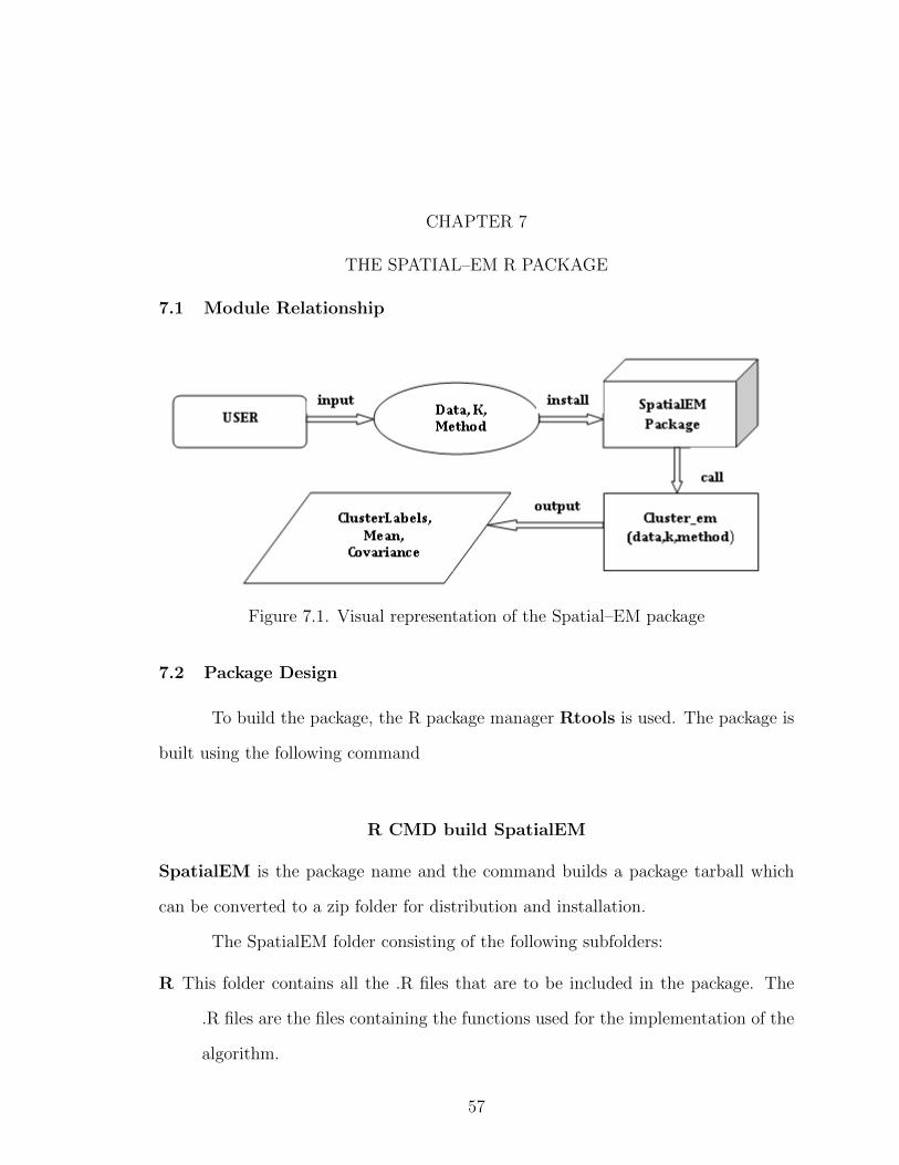
7.1 Module Relationship

Figure 7.1. Visual representation of the Spatial–EM package

7.2 Package Design

To build the package, the R package manager Rtools is used. The package is

built using the following command

R CMD build SpatialEM

SpatialEM is the package name and the command builds a package tarball which

can be converted to a zip folder for distribution and installation.

The SpatialEM folder consisting of the following subfolders:

R This folder contains all the .R files that are to be included in the package. The

.R files are the files containing the functions used for the implementation of the

algorithm.

57

man This folder contains all the .Rd file which are documentationsl for all the func-

tions that are to be exported. An exported function is a function that is visible

to users.

src This folder consists of all compiled codes. In the Spatial–EM package, the only

compiled code is the weighted rank function, which is implemented as a FOR-

TRAN subroutine.

The R package also contains the following text files:

DESCRIPTION As implied, this file gives a general description of the package. It

consists of information such as the author’s name, author’s email, maintainer’s

name, maintainer’s email, package description, to list a few.

NAMESPACE The namespace file is analogous to a permission file. It contains

the functions to be exported and other packages whose functionalities need to

be imported for use by some functions in the package. Only functions declared

with the export command in the namespace file is visible to the user.

LICENSE In addition to the above files, a License file is included that explains the

terms of agreement for using the package.

There are currently three functions accessible to the users. These functions

include:

cluster em This function accepts as input the data, the number of components of

the distribution, and the type of algorithm to be used. The algorithms avail-

able include the Spatial–EM, the Regular–EM, and the Kotz–EM. It returns as

output the predicted labels of the data, and the parameter estimates i.e. the

mean and the covariance of the distribution.

58

k means This function uses the K-means library in the e1071 R package to perform

a K-means clustering of the data provided. It accepts as input the data, and the

number of components, and returns as output the centroids of each component.

confusionMatrix This function accepts as input the true labels, and the predicted

labels, and returns as output the confusion matrix.

To access the package in R, we use the syntax library(SpatialEM) where SpatialEM

is the name of the package.

59

BIBLIOGRAPHY

60

BIBLIOGRAPHY

[1] R implementation of the support vector machine recursive feature extrac-tion (svm–rfe) algorithm. http://www.uccor.edu.ar/paginas/seminarios/

Software/SVM_RFE_R_implementation.pdf. Accessed: 03–12–2015.

[2] A tutorial on clustering algorithms. http://home.deib.polimi.it/matteucc/Clustering/tutorial_html. Accessed: 02–26–2015.

[3] Shaheena Bashir and E.M. Carter. High breakdown mixture discriminant anal-ysis. Journal of Multivariate Analysis, 93(1):102 – 111, 2005.

[4] Scott Shaobing Chen and P. S. Gopalakrishnan. Speaker, environment and chan-nel change detection and clustering via the bayesian information criterion. pages127–132, 1998.

[5] Lian Duan, Lida Xu, Ying Liu, and Jun Lee. Cluster-based outlier detection.Annals of Operations Research, 168(1):0151–168, 2009.

[6] K.T. Fang and T.W. Anderson. Statistical inference in elliptically contoured andrelated distributions. Allerton Press, 1990.

[7] Hironori Fujisawa and Shinto Eguchi. Robust estimation in the normal mixturemodel. Journal of Statistical Planning and Inference, 136(11):3989 – 4011, 2006.

[8] Isabelle Guyon, Jason Weston, Stephen Barnhill, and Vladimir Vapnik. Geneselection for cancer classification using support vector machines. Machine Learn-ing, 46(1-3):389–422, 2002.

[9] D.M. Hawkins. Identification of Outliers. Monographs on applied probabilityand statistics. Chapman and Hall, 1980.

[10] Samuel Kotz. Multivariate distributions at a cross road. In G.P. Patil, S. Kotz,and J.K. Ord, editors, A Modern Course on Statistical Distributions in ScientificWork, volume 17 of NATO Advanced Study Institutes Series, pages 247–270.Springer Netherlands, 1975.

[11] Christopher D Manning, Prabhakar Raghavan, and Hinrich Schutze. Introductionto information retrieval. Cambridge University Press, 2008.

[12] NIST/SEMATECH. http://www.itl.nist.gov/div898/handbook/eda/

section3/eda3666.htm. Accessed: 03–14–2015.

61

[13] W.M. Rand. Objective criteria for the evaluation of clustering methods. Journalof the American Statistical Association, 66(336):846–850, 1971.

[14] J. Ben Schafer, Joseph A. Konstan, and John Riedl. E-commerce recommenda-tion applications. Data Min. Knowl. Discov., 5(1-2):115–153, January 2001.

[15] C. E. Shannon. A mathematical theory of communication. SIGMOBILE Mob.Comput. Commun. Rev., 5(1):3–55, January 2001.

[16] Wikipedia. Clustering analysis. http://en.wikipedia.org/wiki/Cluster_

analysis, 2014. [Online; accessed 28-November-2014].

[17] K. Yu, X. Dang, H. Bart, and Y. Chen. Robust model-based learning viaspatial-em algorithm. Knowledge and Data Engineering, IEEE Transactions on,PP(99):1–1, 2014.

62

oxford approved by: advisor: dr. yixin chen reader: dr...

Documents