Ownership of the Means of Production∗

E. Glen Weyl† Anthony Lee Zhang‡

July 2016

Abstract

Private property creates monopoly power, harming allocative efficiency. Common owner-ship can restore allocative efficiency, but it destroys incentives for investments in the capitalvalue common to all potential owners of an asset. Property rights should thus balance ex-antecapital investment and ex-post allocative efficiency through partial common ownership. Wepropose self-assessed property taxes, with a universal right to force a sale at the self-assessedvalue, as a simple mechanism for implementing partial property rights in dynamic asset mar-kets with many potential buyers. We loosely calibrate a model of self-assessed taxation to theUS housing markets and find that a 5-10% annual tax rate is robustly near optimal, implyingcollectivization of a majority of the capital stock and increasing welfare by approximately6%. However, the simplest application of self-assessed taxation may be to assets with limitedcapital investment opportunities and administratively assigned property rights, such as radiospectrum or internet addresses, where taxes should be set equal to the rate of annual assetturnover.

Keywords: property rights, market power, investment, asymmetric information bargainingJEL classifications: B51, C78, D42, D61, D82, K11

∗We appreciate helpful comments by Evan Kwerel, Eric Posner, seminar participants at the London School ofEconomics, Paul Milgrom’s workshop, Microsoft Research, the University of Chicago Law School and especiallyNicolaus Tideman. All errors are our own.†Microsoft Research New York City, 641 Avenue of the Americas, New York, NY 10011 and Department of

Economics, Yale University; glenweyl@microsoft.com, http://www.glenweyl.com.‡Stanford Graduate School of Business, 655 Knight Way, Stanford, CA 94305; anthonyzhang0@gmail.com.

What is common to the greatest number gets the least amount of care. Men pay most attentionto what is their own; they care less for what is common; or at any rate they care for it only tothe extent to which each is individually concerned.

– Aristotle, The Politics, Book XI, Chapter 3

Property is only another name for monopoly.

– William Stanley Jevons, preface to the second edition of The Theory of Political Economy

1 Introduction

Private ownership of the means of production is perhaps the oldest continually maintaineddoctrine in mainstream economic thought, dating back to the Greek prehistory of the fieldand pervading contemporary thought. For example, Jacobs (1961) and de Soto (2003) arguethe undermining or lack of property rights discourages investment in rich and poor countriesequally. This has led Acemoglu and Robinson (2012) to consistently list property rights asthe leading example of the “inclusive institutions” they argue foster economic development.On the other hand, the founders of contemporary economic analysis (Jevons, 1879; Walras,1896) believed that private property was inherently in conflict with the market principle atthe heart of their systems, because property is monopoly. This argument was formalized byMyerson and Satterthwaite (1981) who show that private property inhibits free competition,thus decreasing the efficiency of allocation, and conversely, Vickrey (1961) showed that undercommon ownership, full allocative efficiency can be achieved through an auction.

In this paper, we propose a simple system of self-assessed taxation that continuously interpo-lates between private and common ownership, trading off the investment incentives from theformer with the allocative benefits from the latter. We loosely calibrate our model to momentsof the US housing markets and argue that a 5-10% annual tax is robustly near optimal. Thisimplies collectivization of approximately two thirds of capital value, and increases average assetuse values by approximately 5.5%. For assets where investment is not important (e.g., radiospectrum) or where investment can be directly rewarded through objective assessment, the taxrate should be higher, approximately equal to the probability of per-period asset turnover.

The role of property rights in incenting agents to invest in assets is an old idea in economics,famously explored in the theoretical literature by Grossman and Hart (1986) and Hart and Moore(1990). Although individuals have incentives for purely “selfish” investment (those that raiseonly that user’s value for using the good) under competitive common ownership (viz. Vickrey’scommons) (Milgrom, 1987; Rogerson, 1992), Che and Hausch (1999) show such schemes typicallydo not give individuals incentives to make investments that might benefit other potential users.1

1Che and Hausch distinguish between “selfish” and “cooperative” investments. Our capital investment is the

1

In particular, common ownership offers zero incentive for an individual to make a “capital”investment that increases the value of the of the asset to all individuals equally, because such aninvestment raises the value of the good to the investing individual’s competitor as much as itraises the value to the investing individual. If the individual does not have an ownership stakein the good, such an investment is a pure waste from her perspective because any competitivemechanism with common ownership must be allocatively neutral in the face of such symmetricincreases in all individuals’ values. Thus, some form of private ownership is crucial to encouragecapital investment.

On the other hand, a separate strand of literature has argued that private property isharmful to allocative efficiency. Myerson and Satterthwaite (1981) show that no mechanismcan achieve fully efficient bargaining between a seller and buyer when the seller has propertyrights. Cramton, Gibbons and Klemperer (1987) show that this failure can be attributed tothe structure of property rights – if both agents have partial ownership of the asset, efficientbargaining is possible.2 This suggests that decreasing the level of private ownership can improvewelfare in market for assets, such as radio spectrum or consumer housing, for which allocativeefficiency is an important concern. However, it is not clear whether such ideas can be applied in adynamic setting when many potential buyers of an asset arrive over time, because there is a largeand evolving potential set of purchasers with whom property rights would need to be shared.Furthermore, as Segal and Whinston (2013) discuss, no existing research combines combines theallocative efficiency costs of private property with the investment efficiency benefits.

In this paper, we suggest self-assessed taxation as a simple tool for interpolating betweencommon and private ownership of property, trading off the benefits of common ownershipfor allocative efficiency and the benefits of private ownership for investment efficiency. In ourbaseline static model, sellers make capital investments in assets that they own, and then setprices at which a buyer can purchase the assets. While investment is efficient under full privateownership, the final allocations of assets are distorted by the market power of the seller. Aself-assessed tax on sellers requires them to pay some fraction of any sale price they announce astax revenue to the community, independently of whether the good is sold. Because Harberger(1965) first proposed this form of self-assessed taxation, we will refer to it as a Harberger tax.In the presence of such a tax, sellers effectively become partially “buyers” as well as sellers;they will tend to announce lower prices, alleviating market power distortions and improvingallocative efficiency. However, sellers pay taxes on the capital value of the assets they own; hence,they do not appropriate the full marginal benefits of their costly capital investments, implyingthat investment is distorted by taxation.

Harberger taxation is fairly simple to implement in practice. Similar systems have been used

sum of a selfish and cooperative investment, because it augments the good’s value to both the investing and otherusers. Any of these types of investment may be synthesized with linear combinations of the other two, but in ourcontext, the classification makes expositing the analysis simpler.

2This idea is further explored by Kaplow and Shavell (1996) and generalized by Segal and Whinston (2011).

2

in a variety of settings dating as far back as ancient Rome,3 although to our knowledge we arethe first to propose using self-assessed taxation to improve allocative efficiency in asset markets.4

Importantly, implementing Harberger taxes only requires identifying the owner of any givenasset, not the large collection of potential buyers of the asset. Additionally, we show in ourTheorem 1 that the tax which maximizes allocative efficiency is particularly simple to determine,as at the optimum it simply equals the probability of asset turnover that it induces.

We then construct a dynamic model of Harberger taxation in which new buyers interestedin acquiring the asset from its current owner repeatedly arrive to the market. We prove theuniqueness of equilibrium for any tax level and that the intuitions from the static model extenddirectly to the dynamic model. However, beyond the basic structure of equilibrium, optimal taxesare challenging to characterize analytically and we thus proceed to numerically calibrate thedynamic model to loosely match moments of the US housing markets. We find that Harbergertaxes in the range of 5-10% are robustly near optimal. This increases the net utility generated bythe asset by approximately 5.5% (or approximately 6.3% of market values), and decreases thetransaction prices of assets in equilibrium by approximately two thirds.

In our calibration, the detrimental effect of Harberger taxes on investment value implies thatthe optimal Harberger tax rate is lower than the probability of asset turnover that it induces.However, for a family of assets for which capital investments are relatively unimportant, such asradio spectrum and internet domain names, optimal tax rates should be substantially higher,approximately equal to the rate of asset turnover that they induce. In addition, if the communitycan observe and directly incent capital investments using objective assessments and investmenttax credits, the negative effects of Harberger taxation on investment can be mitigated, alsoimplying higher optimal tax rates.

In Section 2, we construct our baseline static model and use this to illustrate the fundamentaltrade-offs of our analysis. In Section 3, we introduce our dynamic model and calibration tohousing markets. In Section 4, we discuss various extensions, such as the effect of communityobservability of investment, the effect of taxation on private-value investments, and relaxingour assumptions on the nature of buyers and sellers. In Section 5, we discuss our proposal’srelationship to other work on mechanism design, capital taxation and intellectual property. InSection 6 we discuss applications of our results to different forms of capital. We conclude inSection 7. We present longer and less instructive calculations, proofs and calibration details inan appendix following the main text.

3See Epstein (1997).4The closest prior idea is Tideman (1969)’s demonstration that Harberger taxes tend to increase the probability

of sale, but Tideman does not explicitly model the consequent welfare effects.

3

2 Baseline model

In the baseline model, a seller S holds an asset and makes a single take-it-or-leave-it offer to abuyer B. In the absence of a Harberger tax, S is a monopolist, and announces a price higher thanher value for the asset. If S pays a Harberger tax of τ on p, she has a lower incentive to overstateher valuation. Thus, Harberger taxes alleviate the monopoly distortion and improve allocativeefficiency: the asset more often ends up with the individual with a higher value. However,imposing Harberger taxes on S decreases her incentives to make capital investments in the asset,thus harming investment efficiency.

2.1 Setup

There is a seller S who owns a single asset, and a buyer B. Values of S and B for the asset are,respectively,

vS = η+ γS

vB = η+ γB.

γB ∼ F (·) is a random variable representing heterogeneity in B’s value, which is not observed byS. η is a common-value component; S chooses η > 0, incurring a convex cost c (η) to herself.Both agents are risk neutral.5

For a given η, let 1S, 1B be indicators, which respectively represent whether S and B hold theasset at the end of the game, and let y be any net transfer B pays to S. Final payoffs for S and Brespectively are

US = (η+ γS) 1S − c (η) + y

UB = (η+ γB) 1B − y.

Prior to the beginning of the game, the community decides on a Harberger tax level τ. Then,S and B play a two-period game. In period 1, S chooses η. In period 2, S announces a pricep for the asset, pays taxes pτ to the cadaster, and then B can decide whether to buy the assetby paying p to S. The revenue the cadaster raises is distributed to the broader community in amanner we do not specify here. Since S is a member of a large community, we will ignore anyimpact the revenue raised has on her pricing incentive.6

We solve the game by backwards induction. First, fixing η and τ, we will analyze behavior inthe period 2 price offer game.

5See Tideman (1969) for a partial analysis of the allocative problem that allows for risk aversion.6In fact, even this small issue can be addressed by stipulating that no individual is paid out of the pool of taxes

she paid herself.

4

2.2 Allocative efficiency

For any price p, B’s optimal strategy is to buy the asset if her value is greater than p, that is,if η+ γB > p. Let m ≡ p− η be the markup S chooses to set over the common value η. Theprobability of sale under markup m is then 1 − F (m). Fixing common value η, and Harbergertax level τ, S’s optimal price offer solves:

maxm

(1 − F (m)) (η+m) + F (m) (η+ γS) − τ (η+m) − c (η)

We can change variables to work in terms of sale probabilities. Define q ≡ (1 − F (m)), andM (q) ≡ F−1 (1 − q). S then solves:

maxq

(η+M (q))q+ (η+ γS) (1 − q) − τ (η+M (q)) − c (η)

Note that the socially efficient outcome corresponds to setting M (q) = γS, or equivalentlyq = 1 − F (γS). We can rearrange S’s optimization problem further:

maxq

(M (q) − γS) (q− τ) + (η+ γS) (1 − τ) − c (η)

Only the “variable profit” term (M (q) − γS) (q− τ) depends on the sale probability q. Wecan think of this term as the net trade profits of an agent who owns a fraction 1 − τ of the asset,facing market demand described by M (q). S can always choose q = τ, in which case she makesno net trades and earns zero variable profits. If S chooses q > τ, she is a net seller of a shareq− τ at price M (q) relative to her value γS; likewise, if she chooses q < τ, she is a net buyerof a share τ− q of the asset. Intuitively, if S has value γS higher than the market price M (τ)

at her initial share 1 − τ, or equivalently if S’s quantile among buyer values 1 − F (γS) is lowerthan τ, we expect S to be a net buyer; likewise, we expect S to be a net seller if 1 − F (γS) > τ.In Theorem 1, we formalize this intuition, showing in particular that setting τ = 1 − F (γS) willinduce S to choose q∗ (γS, 1 − F (γS)) = 1 − F (γS), which is the socially efficient outcome.

Theorem 1. (Quantile markup property) q∗ (γS, τ) always lies between τ and 1 − F (γS). Specifically,

1. If τ = 1 − F (γS), then q∗ (γS, 1 − F (γS)) = τ = 1 − F (γS)

2. If τ < 1 − F (γS), then τ 6 q∗ (γS, τ) 6 1 − F (γS)

3. If τ > 1 − F (γS), then 1 − F (γS) 6 q∗ (γS, τ) 6 τ

Proof. For a given γS, τ we consider S’s optimization of the variable profit function:

maxq

(M (q) − γS) (q− τ)

First, suppose that 1 − τ = F (γS).

5

• If S chooses sale probability q = τ, she makes no net trades, and receives 0 variable profit.Moreover, the markup is M (q) = F−1 (1 − τ) = γS, so that M (q) = γS.

• If S chooses a higher sale probability, so that q− τ > 0, we have M (q) 6 γS, so variableprofits (M (q) − γS) (q− τ) 6 0. In words, S becomes a net seller at a price lower than hervalue.

• If S chooses a lower sale probability, so that q− τ < 0, we have M (q) > γS, so variableprofits (M (q) − γS) (q− τ) 6 0. In words, S becomes a net buyer at a price higher thanher value.

Hence, the optimal strategy for S is to choose q = τ. Suppose now that τ < 1 − F (γS).

• Suppose we raise the tax rate to 1− F (γS). By the first part of the claim, q∗ (γS, 1 − F (γS)) =

1 − F (γS). The variable profit function is supermodular in τ and q, so if we lower the taxrate from 1 − F (γS) to τ, q∗ must decrease, so q∗ (γS, τ) 6 1 − F (γS) .

• If we increased γS to F−1 (1 − τ), again by the first part of the claim, we would haveq∗(F−1 (1 − τ) , 1 − τ

)= 1 − τ. The variable profit function is supermodular in −γS and q,

hence if we lower S’s value from F−1 (1 − τ) to γS, q∗ must increase, so q∗ (γS, τ) > 1 − τ.

The third part of the claim, for τ > 1 − F (γS), follows symmetrically to the second.

An important consequence of Theorem 1 is that, for any given seller value γS, the allocativelyoptimal tax can be found without knowledge of the distribution F (·): if the community iterativelysets the tax equal to the current probability of sale, τk+1 = q? (τk), the tax τk will converge tothe efficient probability of sale 1 − F (γS).

To quantify these comparative statics we now assume F (·) is twice continuously differentiable.S’s first-order condition is

M ′ (q) (q− τ) + (M (q) − γS) = 0,

so that by the Implicit Function Theorem,

∂q?

∂τ=

M ′ (q?)

2M ′ (q?) +M ′′ (q?) (q? − τ)=

1

2 +M ′′(q?)(q?−τ)

M ′(q?)

=1

2 −M ′′(M−γS)

(M ′)2

,

where the last equality invokes the first-order condition and drops arguments. Cournot (1838)showed that this quantity equals the pass-through rate ρ (q?) of a specific commodity tax intoprice; see Weyl and Fabinger (2013) for a detailed discussion and intuition. ρ is closely relatedto the curvature of the value distribution; it is large for convex demand and small for concavedemand. It is strictly positive for any smooth value distribution and is finite as long as S is at astrict interior optimum.7

7Myerson (1981)’s regularity condition is sufficient but not necessary for this second-order condition, as we showin Appendix A.1.

6

The marginal gain to social welfare from a unit increase in the probability of sale is equal to thegap between γB and γS, because the tax raised is simply a transfer. This gap is, by construction,(M (q?) − γS). Thus, the marginal allocative gain from raising τ is (M (q?) − γS) ρ (q

?) or(M− γS) ρ for short.

Note that (M− γS) ρ is 0 at q = 1 − F (γS), so the first-order social welfare gain from taxationapproaches 0 as we approach the allocatively optimal tax of 1 − F (γS). On the other hand, whenτ = 0, we have (M− γS) ρ > 0 and increasing τ creates a first-order welfare gain.

2.3 Investment efficiency

Note the variable profits defined in the previous subsubsection were independent of η. On theother hand, the sunk profits, (1 − τ)η− c (η) , depend on η. Because this component is entirelyseparable from the other component, regardless of what happens in the second stage of thegame, S finds it optimal to choose η such that:

c′ (η) = 1 − τ.

We can define the investment supply function Γ (·) as:

Γ (s) ≡ c′−1 (s) .

The value of a unit of investment η is always 1, so the socially optimal level of investment isΓ (1), whereas investment is only Γ (1 − τ) when the tax rate is τ. By strict convexity of c, Γ isstrictly increasing, so the higher the tax, the more downward distorted the investment.

Again turning to the quantitative side, the marginal increase in investment from a risein τ is Γ ′ = 1

c ′′ by the inverse function theorem. The social value of investment is always 1,whereas S only invests up to the point where c ′ = 1 − τ. Thus, the marginal distortion fromunder-investment is τ. Thus, the marginal social welfare loss from raising τ is Γ ′τ = τ

1−τΓεΓ ,where εΓ is the elasticity of investment supply. Note that as τ→ 0, this investment distortiongoes to 0, so that there is no marginal investment distortion near the investment optimum ofzero tax, whereas at any other tax (such as the allocatively efficient tax level 1 − F (γS)), there isa strictly positive marginal investment distortion, as long as c does not have a convex kink inthe relevant neighborhood.

2.4 Tradeoff between allocative and investment welfare

Fixing S’s value γS, the socially optimal level of property rights balances the cost of taxation forinvestment efficiency with its benefit (below 1 − F (γS)) to allocative efficiency. It thus solves a

7

Figure 1: Allocative, Investment, and Total Welfare vs Tax

classic optimal tax formula:

τeff1 − τeff

=(M (q? (γS, τeff)) − γS) ρ (q? (γS, τeff))

Γ (1 − τeff) εΓ (1 − τeff). (1)

Under weak additional regularity conditions we discuss in Appendix A.1, this equationhas a unique solution. The left-hand side is a monotone-increasing transformation of τ thatappears frequently in elasticity formulas in the optimal tax literature; see, for example, Werning(2007). The right-hand side is the ratio of two terms: the allocative benefit of higher taxesand the investment distortion of higher taxes. The allocative benefit equals the product of themark-up and the pass-through rate, whereas the investment distortion equals the product of theequilibrium investment size and its elasticity with respect to 1 − τ. By the logic of the previoussubsections, τeff ∈ (0, 1 − F (γS)).

Proposition 1. The optimal tax rate τeff that maximizes social welfare is strictly positive and strictlybelow 1 − F (γS), and satisfies:

τeff1 − τeff

=(M− γS) ρ

ΓεΓ.

Figure 1 graphically illustrates the tradeoff between allocative and investment welfare.Allocative welfare increases monotonically in τ on the interval τ ∈ [0, 1 − F (γS)], with slope 0 atτ = 1 − F (γS). Investment welfare decreases monotonically in τ, with slope 0 at τ = 0. Thus,τeff always lies strictly in the interior of the interval (0, 1 − F (γS)).

8

3 Dynamic model

In this section, we construct a dynamic model of Harberger taxation, and show that the coreintuitions of the static model extend to this more general setting. This allows us to study theeffect of Harberger taxation on turnover rates and the stationary distribution of values, as well asthe influence of Harberger taxation on asset prices. We calibrate the model loosely to features ofUS housing markets, and show that Harberger taxes in the range of 5-10% robustly increase totalvalue, and that larger Harberger taxes can achieve a large fraction of total possible allocativewelfare.

3.1 Model

3.1.1 Agents and Utilities

Time is discrete, t = 0, 1, 2 . . .∞. All agents discount utility at rate δ. There is a single asset,which an agent S0 owns at time t = 0. In each period, a single buyer Bt arrives to the marketand bargains with the period-t seller St to purchase the asset, through a procedure we detail inSubsubsection 3.1.2 below. Hence, the set of agents is A = {S0,B0,B1,B2 . . .}. We will use St asan alias for the period-t seller, who may be a buyer Bt′ from some period t′ < t. We will oftenuse A to denote a generic agent in A .

In period t, agent A has period-t use value γAt for the asset. The values of entering buyersγBtt are drawn i.i.d. from some distribution F. Values evolve according to a Markov process:for any agent A with period-t usage utility γAt , her use value in the next period γAt+1 is drawnaccording to the transition probability distribution G (γt+1 | γt).

Assumption 1. G (γ | γ) = 1 ∀γ, that is, γt+1 6 γt with probability 1.

Assumption 2. γt > γ′t implies G (γt+1 | γt) >FOSD G (γt+1 | γ′t).

Assumption 3. G (γ′ | γ) is continuous and differentiable in γ for any γ′.

Assumptions 1 and 2 imply that, for any given agent, use values decay uniformly over time,in the sense that future values are always lower than current values, and higher current valuesimply uniformly higher future values in the sense of stochastic dominance. Assumption 3guarantees that the value decay process is smooth.

In any period, there is a single owner of the asset. Let 1At denote agent A being the owner ofthe asset in period A. Agent A’s utility for ownership path 1At and utility path γAt , is:

∞∑t=0

δt[1At γ

At + yAt

]Where, yAt is any net monetary payment made to agent A in period t.

9

To avoid dealing with repeated strategic interactions, after the period in which agent Aarrives to the market as a buyer, we will allow agent A to remain in the market only so long as1At = 1; once 1At = 0, agent A leaves the market forever. Thus, in each period t, only two agentsexist in the market: the period t seller St, and the arriving buyer Bt. Any pair of agents interactsat most once.

A (possibly random) allocation rule Φ (ht) determines in each time t, history ht whether toallocate the good to St or Bt. Intuitively, since Assumption 2 states that higher present valuesimply uniformly higher future values, a social planner aiming to maximize average use valuesshould assign the asset to whichever of St,Bt has higher current-period value in any givenperiod. This is formalized in the following proposition.

Proposition 2. The socially optimal allocation rule Φ (·) allocates the good to whichever of {St,Bt} hashigher use value γt in every period t.

Proof. See Appendix Section A.2.

3.1.2 Game

The community chooses some Harberger tax level τ, constant for all time. For any tax level τ,we will define the following dynamic Harberger tax game. At t = 0, agent S0 owns the asset, andobserves her own use value γS0

t for the asset. In each period t:

1. Buyer arrival: Buyer Bt arrives to the market; his use value γBtt is drawn from F (·), and isobserved by himself but not the period-t seller St.

2. Seller price offer: Seller St makes a take-it-or-leave-it price offer pt to buyer Bt, andimmediately pays tax τpt to the community.

3. Buyer purchase decision:

• If Bt chooses to buy the asset, she pays pt to St. Bt becomes the period-t asset owner,1Btt = 1, and enjoys period-t use value γBtt for the asset. Bt becomes the seller inperiod t+ 1, that is, St+1 ≡ Bt. Seller St receives payment pt from Bt, and seller Stleaves the market forever, with continuation utility 0.

• If Bt chooses not to purchase the asset, St becomes the period-t asset owner, 1Stt = 1,and she enjoys period-t use value γStt . St becomes the seller in period t+ 1, that is,St+1 ≡ St. Buyer Bt leaves the market forever, with continuation utility 0.

4. Value updating: γSt+1t+1 , the period t+ 1 value for seller St+1, is drawn from G

(γt+1 | γ

St+1t

)according to her period-t value γSt+1

t .

10

3.1.3 Equilibrium

Equilibrium in the dynamic Harberger tax game requires that, in all histories, all sellers makeoptimal price offers, and all buyers make optimal purchase decisions. Since τ, F, G are constantover time, the problem has a Markovian structure: the optimal strategies of buyers and sellersmay depend on their types γStt ,γBtt respectively, but not on the period t. Hence we can applydynamic programming techniques, characterizing equilibria of the game by a stationary valuefunction V (γ) which describes the value of being a type γ seller in any given period.

In any period t, we can think of seller St as choosing a probability of sale qt, where buyersin period t make purchase decisions according to the inverse demand function p (qt). If thecontinuation value in period t + 1 for seller type γt+1 is V (γt+1), the seller’s optimizationproblem in period t is:

maxqt

qtp (qt) + (1 − qt)[γt + δEG(γt+1|γt)

[V (γt+1) | γt]]− τp (q)

Simplifying and omitting t subscripts, optimality for the seller requires V (γ) to satisfy thefollowing Bellman equation:

V (γ) = maxq

(q− τ)p (q) + (1 − q)[γ+ δEG(γ′|γ)

[V(γ′)| γ]]

(2)

Buyer optimality pins down the relationship between p (·) and V (·). If buyer Bt with valueγt purchases the asset, he receives value γt in period t, and then becomes the seller in periodt+ 1, receiving utility δV

(γBtt+1

). Hence the period-t willingness-to-pay of buyer type γt is:

WTP (γt) = γt + δEG(γt+1|γt)[V (γt+1) | γt]

Thus, in equilibrium, optimality for the buyer implies that the inverse demand function p (·)satisfies:

p (q) ={p : Pγ∼F(·)

[γ+ δEG(γ′|γ)

[V(γ′)| γ]> p

]= q}

(3)

Fixing τ, a value function V (·) which satisfies equations (2) and (3) defines an equilibrium ofthe dynamic Harberger tax game.

Theorem 2. For any τ, F, G satisfying our assumptions, there exists a unique equilibrium of the dynamicHarberger tax game.

Proof. We prove this theorem in Appendix Section A.3, where we also describe a numericalprocedure that solves for the unique equilibrium for any τ.

The following theorem states that the “net trade” intuition from the static Harberger taxgame applies exactly to the dynamic case.

11

Theorem 3. (Dynamic quantile markup property) In any τ-equilibrium of the dynamic Harbergertaxation game, Theorem 1 holds, that is, the optimal sale probability function q∗ (γ) satisfies:

1. For type γ such that τ = 1 − F (γS), we have q∗ (γ) = τ = 1 − F (γ)

2. Types γ with τ < 1 − F (γS) are net sellers, that is, τ 6 q∗ (γ) 6 1 − F (γ)

3. Types γ with τ > 1 − F (γ) are net buyers, that is, 1 − F (γ) 6 q∗ (γ) 6 τ

Proof. This follows from the more general Claim 2 in Appendix Subsection A.3.

Together, these theorems demonstrate that the basic intuitions of the static model carry overto the dynamic Harberger tax game. However, the dynamic game is generally not analyticallysolvable, and comparative statics of outcomes with respect to τ are difficult to calculate analyti-cally. Instead, we proceed in Subsection 3.2 by calibrating the dynamic Harberger tax game torealistic parameters, numerically calculating the equilibria for different levels of τ, and studyingthe effect of changing τ on steady-state asset use values and other equilibrium outcomes.

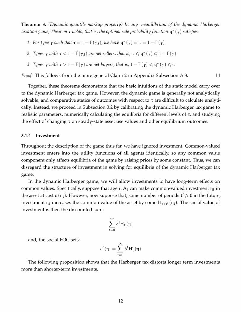
3.1.4 Investment

Throughout the description of the game thus far, we have ignored investment. Common-valuedinvestment enters into the utility functions of all agents identically, so any common valuecomponent only affects equilibria of the game by raising prices by some constant. Thus, we candisregard the structure of investment in solving for equilibria of the dynamic Harberger taxgame.

In the dynamic Harberger game, we will allow investments to have long-term effects oncommon values. Specifically, suppose that agent At can make common-valued investment ηt inthe asset at cost c (ηt). However, now suppose that, some number of periods t′ > 0 in the future,investment ηt increases the common value of the asset by some Ht+t′ (ηt). The social value ofinvestment is then the discounted sum:

∞∑t=0

δtHt (η)

and, the social FOC sets:

c′ (η) =∞∑t=0

δtH′t (η)

The following proposition shows that the Harberger tax distorts longer term investmentsmore than shorter-term investments.

12

Proposition 3. In any τ-equilibrium of the dynamic Harberger taxation game, all agents choose aconstant level of investment η such that:

c′ (η) =∞∑t=0

δt (1 − τ)t+1H′t (η)

Proof. See Appendix A.4.

3.2 Calibration

3.2.1 Specification and moment matching

In this section, we study a computational simulation of dynamic Harberger taxation looselycalibrated to US housing markets.

Our dynamic Harberger taxation game has two main unknowns: the distribution of enteringbuyer values F (γ), and the transition probability distribution G (γ′ | γ). In addition, we have tochoose the discount rate δ, and the investment cost function c (η) and benefit functions Ht (η).

We will assume that the distribution of entering buyer values F (·) is lognormal, with logmean normalized to 0. The log standard deviation parameter σ then serves the role of aspread parameter, controlling the amount of idiosyncratic dispersion in values, which therebydetermines the social loss from allocative inefficiency. We model the transition probabilitydistribution G (γ′ | γ) as follows: given an agent in period t with value γt at the F−1 (γ)thquantile of F (·), her period t+ 1 value γt+1 is calculated by drawing a value ψ from the betadistribution with parameters [κβ, κ (1 −β)], then setting γt+1 equal the ψF−1 (γ) quantile of F (·).The result is that values decay in quantile terms, with expected quantile decay rate β. The shapeparameter κ, which represents the prior sample size in the “Bernoulli prior” interpretation ofthe beta distribution, is somewhat arbitrary, and we use κ = 10 in our simulations.

We are left with two parameters to determine: the log standard deviation σ of F, and thequantile decay rate β of G. To match these parameters, we target two moments of housingmarkets. Willekens et al. (2015) finds that, in the Danish housing market, the idiosyncraticvariance in house prices is at least 10%. We will refer to this moment as sdmean, and we willmatch it by requiring the standard deviation of transaction prices in equilibrium for τ = 0 toequal sdmean. Using American Housing Survey data, Emrath (2013) estimate that the averagehouse is sold approximately once every 13 years. We will refer to this moment as saleprob, andwe will match it by requiring the average sale probability in each period in the τ = 0 equilibriumto equal saleprob.

Intuitively, under our parametrization, increasing the quantile decay rate β increases theprobability of efficient sale, and hence should increase the efficient tax level. Increasing thelognormal standard deviation σ increases the dispersion of values about its mean; this should

13

Figure 2: Stationary Use Value Distributions vs τ

increase the dispersion of prices, with a smaller effect on the probability of sale. Hence, weshould expect that the saleprob moment is matched mostly by the decay rate β, whereas thesdmean moment is matched more by σ. We confirm these intuitions in Figure 4, which wediscuss in Section 3.2.2. However, as both σ and β simultaneously influence the probability ofsale and the dispersion of prices, we jointly choose σ and β in order to match the saleprob andsdmean moments.

On the investment side, we will assume that investment has geometrically depreciating valueover time: Ht (η) = θtη, θ < 1. For our calibrations, we will set θ = 0.85, which is similarto numbers used in the literature on capital depreciation (Nadiri and Prucha, 1996). We willassume the investment cost function is quadratic, c (η) = η2

2g , and we will choose g such that thetotal value from investment is some fraction invfrac of the mean allocative welfare in stationarydistribution at τ = 0. Glaeser and Shapiro (2003) show that ownership in a neighborhoodroughly influences housing values by 25%, hence we use invfrac = 0.25 in our calibration. InAppendix B.2, we analytically solve for the equilibrium investment level and investment welfarefor any value of τ.

Finally, we will use the standard choice of δ = 0.95. In Appendix B.1, we describe furtherdetails of the numerical procedure we use to analyze the game and solve for equilibria.

3.2.2 Results

In Figure 2, we show the stationary distribution of use values vs. tax rate τ. As τ increases from0 to .15, the stationary distribution puts more mass on relatively higher values of γ. Howevernote that a further increase to .2 has more mixed effects, decreasing the mass on the veryhighest values and on the lowest values, as the higher rate of turnover it induces eliminates

14

inefficiently low values but also excessively encourages sales by the highest value sellers. In factthis phenomenon even emerges at lower tax rates, but is so modest as to make little difference.This is why we will find that allocative efficiency is maximized at a 15% tax rate.

In Figure 3, we show the behavior of various parameters as we change τ. In the topmost panel,we show the behavior of allocative, investment and total welfare with respect to τ. Allocativewelfare is maximized at approximately τ = 0.15, and this value of τ achieves over 80% of welfaregains relative to the social planner’s optimum. Note that this is despite the fact that theoreticallythis could be a very small fraction of the greatest possible gains as seller values, and thus efficientprobabilities of sale, are very heterogeneous. If we consider investment welfare as well, theoptimal tax is τ = 0.072, and this increases total welfare by 5.5%, which is 6.3% of the averageasset transaction price with pure private ownership. However even this reduced tax achievesmore than 70% of the maximum allocative welfare gains. Thus the limits on allocative gainsplaced by heterogeneous seller values (viz. the imperefctions of the coarse Harberger tax relativeto a more optimal allocative mechanism) and investment distortion are roughly comparable.Asset prices under the optimal tax are approximately 37% of asset prices under pure privateownership.

In the second panel of Figure 3 we show the behavior of quantile markups and sale frequencywith respect to τ. Average quantile markups decrease and sale frequency increases as we raise τ.The average quantile markup is 0, and the sale frequency is equal to the tax rate, when τ is setequal to the efficient probability that the good turns over, similar to the intuition in the staticmodel from Theorem 1. However, the allocatively optimal tax is slightly lower than the efficientprobability of sale, likely because the right-skew of the lognormal distribution means that thelosses from excessive turnover shown in Figure 2 by high value sellers outweigh the gains fromeliminating inefficiently low turnover rates by low value sellers.

In the third panel of Figure 3 we show the behavior of various stock/flow quantities aswe vary τ. Importantly, asset prices rapidly decrease and tax revenues rapidly increase as weincrease τ. Intuitively, if agents have to pay tax τ every period, this is roughly equivalent todiscounting by rate δ (1 − τ); thus, increasing τ has a similar effect to increasing discounting, andrapidly lowers asset prices. The net present value of tax revenues greatly exceeds the price ofthe asset even for relatively small values of τ, supporting the interpretation that Harberger taxeseffectively act by continuously decreasing the degree of private ownership of assets, movingtowards a “partial rental” system from the community.

15

Figure 3: Comparative statics vs τ

16

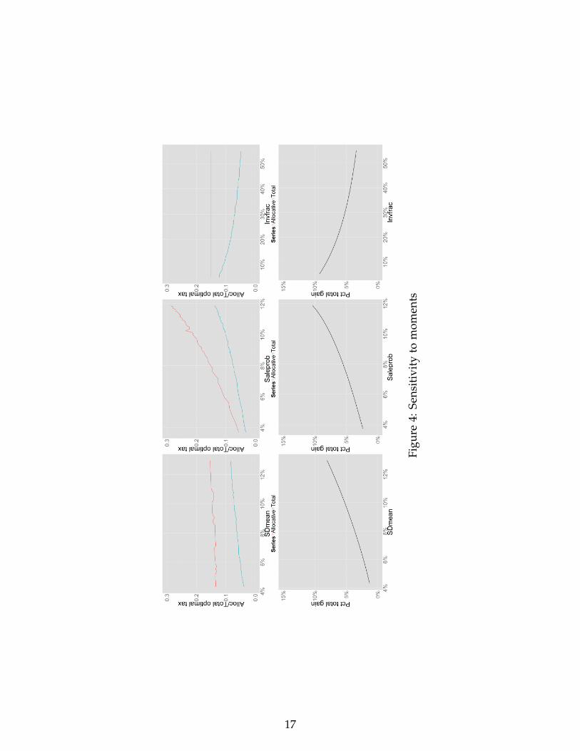
Figu

re4:

Sens

itiv

ity

tom

omen

ts

17

In Figure 4, we vary the input moments used in the calibrations, and show that allocative/totaloptimal taxes and total welfare gains depend on the input moments in intuitive ways. Changingthe sdmean moment moves the percent total welfare gain, with a relatively small effect on theoptimal tax rate. Changing the saleprob moment moves both optimal taxes and welfare gains.Changing the invfrac moment lowers the total optimal tax relative to the allocatively optimaltax. While optimal taxes and their associated welfare gains vary across all of these calibrations,note that the optimal tax almost never falls below 5% or rises above 10% and when it does exitthese bounds it does so by a very small amount. As this suggests, we find that over the fullrange of parameters we try any tax in the range of 5-10% is superior to full private ownershipand is quite close to optimal.

4 Extensions

In this section, we consider several extensions that investigate the robustness of our analysis inthe baseline case as well as enrich it in various directions. For simplicity, all these extensionsbuild off of the static model of Section 2, rather than the dynamic model of the previous section.

In Subsection 4.1, we show that if the community is able to observe and directly incent theseller to make common-valued investments, it can alleviate the investment efficiency losses fromHarberger taxation, leading to higher optimal tax levels. Subsection 4.2 shows private-valuedinvestments by the seller are efficient in our mechanism, regardless of the level of the Harbergertax. In Subsection 4.3, we show that increasing competition on the buyer side lowers the optimallevel of the Harberger tax.

4.1 Partial observability

In our analysis above, the public cannot directly reward investments made by individuals, andthus distorts investment when taxing self-assessed property. In some cases, though, the publicmay be able to directly reward capital investments. After all, the leading property of capitalinvestments is that they affect the objective value to all individuals and not just to the idiosyncraticvalue of the seller. Furthermore, for the purposes of imposing more traditional property taxesfor real estate agents or other paid experts, making an objective appraisal of the market value ofa property is common practice.

Beyond these common practices, a number of mechanisms could be used to elicit valuationsfrom private agents, such as keeping cadastral values secret but having individuals offer bids onthem that would be accepted upon exceeding cadastral value but that would also be used toestimate capital appreciation. Although such schemes could be gamed through collusion betweenpotential buyers and the seller, law enforcement may be able to discourage such manipulations.Additionally, Levmore suggests other schemes for eliciting competing assessments, and the

18

literature on mechanism design is continually developing more elaborate methods for elicitationin circumstances like these; see, for example, Cremer and McLean (1988).

If some mix of objective appraisal and such elicitation mechanisms could provide at least anoisy signal of capital value, the public may be able to directly reward investments through atax deduction for investment value and thus avoid the investment distortion from the Harbergertax, which in turn raises its optimal rate closer to the allocatively efficient level. This argumentcaptures some of Hayek (1945)’s intuition that local knowledge is what limits the prospects ofcommon ownership. In this subsection, we formalize this intuition by following the analysis ofBaker (1992) to construct optimal direct property subsidies to mitigate the moral hazard problemcreated by Harberger taxation.

As before, suppose S chooses η at cost c (η). However, now suppose common value υ isdetermined by

υ = ζη,

where ζ is a random variable representing the value of investment in different states of theworld. There is local information about ζ; that is, S and B both observe ζ prior to investment, butthe public does not.8

The community can observe η and a signal ξ. Prior to period 1, the community can choosean incentive scheme ηψ (ξ), meaning that if the community observes ξ, it will pay S some amountψ (ξ) for each unit η of investment S makes. This policy is simply a negative property (propertysubsidy) based on an objective appraisal of υ.

Fix a realization of the signal value ξ. If the community chooses reward function ψ (ξ)η,and the Harberger tax rate is τ, investment level Γ (ψ (ξ) + (1 − τ) ζ) will be induced. Forexpositional simplicity, we now focus on the case when costs of investment are quadratic andthus Γ is linear: η (ζ) = gζ for some g > 0, or, equivalently, that cost is c (γ) = γ2

2g . Baker (1992)uses Taylor approximations to show that similar conclusions hold for more general investmentcost functions.

Given any choice of ψ (ξ), S chooses investment:

Γ (ψ (ξ) + (1 − τ) ζ) = g (ψ (ξ) + (1 − τ) ζ) .

Hence, for a fixed τ, the optimal ψ solves pointwise over realizations of ξ the maximizationproblem:

maxψ

E

[g (ψ (ξ) + (1 − τ) ζ) ζ−

(g (ψ (ξ) + (1 − τ) ζ))2

2g| ξ

].

8An alternative formulation of this model is that the cost of investment is uncertain and is known to the sellerand buyer, but the community only observes a noisy signal of the cost. Although this interpretation is more naturalin many settings, we focus on the “investment value” interpretation to stay closer to Baker’s analysis and because itis simpler to present.

19

This program has the simple linear solution ψ (ξ) = τE (ζ | ξ), which induces investment

g (τE (ζ | ξ) + (1 − τ) ζ) = g (E (ζ | ξ) + (1 − τ) (ζ− E (ζ | ξ))) .

Investment is thus equal to the conditional expectation of investment value conditional on thesignal ξ, plus a multiple 1 − τ of the deviation ζ− E (ζ | ξ) from the conditional mean. Forhigher values of τ, investment is closer to the conditional mean.

The social welfare loss from this noisy estimation is

IVL =τ2

2gE[ζ2 − (E (ζ|ξ))2

]=τ2

2g(

1 − r2)Var (ζ) ,

where r2 = E[(E (ζ | ξ))2

]is the fraction of the variance in ζ that is predictable by ξ. If we take

the derivative with respect to τ, we get

dIVL

dτ= −τg

(1 − r2

)Var (ζ) . (4)

As r2 increases, dIVLdτ decreases in magnitude, and the socially optimal choice of the Harbergertax given by equation

τ?

1 − τ?=

(M− γS) ρ

τg (1 − r2)Var (ζ)

moves closer to the allocatively efficient level (1 − F (γS)). Thus, to the degree that the public canobserve and reward capital investment, the detrimental effect of Harberger taxes on investmentefficiency diminishes, and the optimal Harberger tax level is higher. This finding is consistentwith Lange (1967)’s argument that the improvement of observation and computation throughthe improvement of information technology would increasingly make common ownership ofthe means of production feasible.9 In fact, ongoing work by a team of researchers led by NikhilNaik, of which Naik et al. (2015) is a preliminary output, is attempting to automate high-qualityproperty value assessment using Google’s Streetview images combined with computer visionand machine learning.

9 In particular, in this limit, George (1879)’s argument for the taxation of land value while allowing people tokeep investment value (see Subsection 5.2 below) becomes possible and thus all land, and no investment should betaxed. However, in contrast to this argument for full common ownership, our analysis suggests that for any r2 < 1,for any seller type γS, the optimal Harberger tax approaches only 1 − F (γS) and not 1. Thus even as informationtechnology improves, fully common ownership may not be desirable. However, note that our calculations inSubsection 3.2 above suggest that a tax at the allocatively efficient turnover rate would likely expropriate theoverwhelming majority of the value of private capital. For example, at a 5% discount rate, an allocatively efficientturnover rate of 30% would imply the expropriation of 85% of private capital value. Furthermore, for r2 = 1, a fullcommon ownership is efficient as well, so in a more general environment, and at the true limits of informationtechnology or elicitation mechanisms described above, Lange’s argument may hold up in its simpler form.

20

4.2 Selfish investments

Thus far, we have assumed the seller’s investment only affects the common value of the good.Here, we show that if the seller can make pure private-value investments, that is, investmentsthat affect only her value for the good, these investments are efficient, conditional on the finalprobability that the seller holds the asset. This efficiency guarantee is true regardless of the levelof the tax, which is why we largely ignore such selfish investments in our analysis above.

Suppose S can invest in increasing her private value for the good: she can increase her ownuse value for the good by λ at cost c (λ). As before, B has value η+ γB for the good, and allother features of the game are identical to those in Section 2. Fixing γS and λ, S’s second stageprofits are once again:

πS (λ,γS, τ) ≡ maxqp (q)q+ (η+ γS + λ) (1 − q) − p (q) τ.

Let q∗ (τ,γS) represent S’s choice of q for any given τ,γS. In the investment stage, S choosesλ to maximize πS (λ,γS, τ) − c (λ). But, using the envelope theorem, we have that

dπS (λ,γS, τ)dγ

=∂

∂λ[p (q∗ (τ,γS))q∗ (τ,γS) + (η+ γS + λ) (1 − q∗ (τ,γS)) − p (q∗ (τ,γS)) τ]

= 1 − q∗ (τ,γS) .

Hence, the first-order condition for S’s choice of private-valued investment λ is

c′ (λ) = 1 − q∗ (τ,γS) .

This equation defines the constrained efficient level of investment, conditional on S keepingthe asset with probability 1 − q∗ (τ,γS). Thus, Harberger taxation does not directly affectselfish investment efficiency. The only impact of Harberger taxes on such selfish investments isindirectly, through the probability of sale. For example, with absolute private property, selfishinvestments will tend to be too high relative to the social optimum, because q? is depressedbelow 1− F (γS). Thus, with pure private ownership, individuals will tend to invest in becomingexcessively “attached” to their possessions relative to an optimal world where possessions turnover more frequently, as Blume, Rubinfeld and Shapiro (1984) first observed. However, thisdistortion occurs only because of the change in the turnover rate and not directly because of thetax.

A few more informal observations are in order:

1. Our analysis shows that no issue of “hold-up” in the spirit of Grossman and Hart (1986);Hart and Moore (1990, 1988) with purely selfish investments exists in this model. Thereason is that the investor (the seller) makes a take-it-or-leave-it offer that the buyer thus

21

cannot appropriate the seller’s investment. This property would not hold if the buyermade a take-it-or-leave-it offer. However, the very structure of the Harberger tax makes aseller offer the natural bargaining protocol, so we don’t consider this a serious concern.

2. Milgrom (1987) and Rogerson (1992) show that a Vickrey auction with common ownershipor efficient bargaining through the similar Expected Externality mechanism (Arrow, 1979;d’Aspremont and Gerard-Varet, 1979) implies ex-ante selfish and privately observedinvestments are efficient. Our result indicates this result is driven entirely by the factthat these protocols lead to efficient allocations and not at all by the impact of theseprotocols on investment decisions conditional on investments, given that privacy ensuresone’s bargaining partner cannot change his offer, even if the investor does not make atake-it-or-leave-it offer.

3. A natural concern with Harberger taxation is that individuals may try to “sabotage” thevalue of their goods to others. However, our analysis shows that they never have a localincentive to do this as long as the tax rate is weakly below the turnover rate. To see this,note that sabotage is equivalent to a negative unit of capital investment plus a positiveunit of selfish investment. The value derived from such an investment is, by our aboveanalysis, 1 − q? − (1 − τ) = − (q? − τ). Intuitively as long as τ < q? the price the sellersets is weakly above the monopoly price and thus the seller benefits when her propertyis taken, though not as much as were τ = 0. Thus she would not choose to sabotage herproperty in equilibrium.10

4. One objection to Harberger taxation is that individuals with high idiosyncratic utilitiesfor assets must pay a high tax to avoid takings. To the extent that such idiosyncraticattachments are the result of random shocks an individual may experience, taxing awaythe benefits of such shocks could be either an advantage or disadvantage of Harbergertaxation, depending on how this random gain in idiosyncratic utility interacts with themarginal value of consumption and thus whether individuals would like to insure againstsuch shocks (as the Harberger tax effectively does). Regardless, our risk-neutral frameworkdoes not adequately capture these issues.

However, to the extent that such attachment is partially under the control of the owner,this may actually be an additional benefit of Harberger taxation. In particular, commonexperience suggests individuals tend to form much stronger attachments to objects that donot decay than to those that are durable, and to objects they own versus those they rent.Because of monopoly distortions, property tends to turn over much less frequently than issocially optimal. Thus, alleviating monopoly distortions may optimally lead individuals to

10Note this argument is local and it could be possible that a joint global deviation to a very low price and extremesabotage could be optimal in some cases. Levmore (1982) provides a detailed plan for how such extreme sabotagecould be avoided.

22

become less attached to their possessions. This excessive attachment to material possessionsis one of the principal flaws many religious and social thinkers (especially from theBuddhist tradition) perceive in capitalist societies. Therefore, unsurprisingly thoughheartening, moving optimally toward common ownership would tend to alleviate suchattachment.

4.3 Many buyers

Our analysis above assumes that there is a single potential buyer of the asset. In many realisticcases, several bidders may be competing to buy the asset. In this subsection, we analyze theeffect of buyer-side competition on the optimal Harberger tax rate using a simple auction model.

Suppose the asset belongs to the seller S, and assume for simplicity that γS = 0. There aremultiple buyers B1 . . .Bn, with values drawn i.i.d. from distribution F. The asset is sold in asecond-price auction, where S can set a reserve price p. S pays a tax on the reserve price p. Lety1 represent the highest bid, and let y2 represent the second-highest bid. S’s objective function is

πS = y21y1,y2>p + p1y1>p>y2 + η1y1,y2<p − pτ.

Taking expectations over y1,y2 and then taking derivatives with respect to p yields

dE [πS]

dp= P (y1 > p > y2) − τ−m

dP (y1,y2 < p)

dp,

where, as in Section 2, we define the markup m ≡ p − η. Substituting for the probabilityexpressions, the derivative becomes

dE [πS]

dp= nFn−1 (p) (1 − F (p)) − τ−mnFn−1 (p) f (p) .

If we set this to 0, we get

τ = nFn−1 (p) (1 − F (p)) −mnFn−1 (p) f (p) . (5)

Allocative efficiency is achieved when p = η and thus m = 0, which requires

τ = nFn−1 (η) (1 − F (η)) .

As n→∞, this expression goes exponentially to 0. Thus, the allocatively optimal Harbergertax goes to 0 as competition grows. This conclusion is intuitive, given the follow-up to Jevons(1879)’s quote in our epigraph:

But when different persons own property of exactly the same kind, they become subject to the

23

important Law of Indifference...that in the same open market...there cannot be two prices forthe same kind of article. Thus monopoly is limited by competition, and no owner, whether oflabour, land, or capital, can, theoretically speaking, obtain a larger share of produce for it thanwhat other owners of exactly the same kind of property are willing to accept.

Larsen (2015) confirms this intuition empirically, and shows that sufficient competition in themarket for used automobiles (if they are put up for an auction with dozens of bidders) limits themarket-power distortion from property to 2%-4% of first-best allocative efficiency. Thus, in verycompetitive environments, or any environment where buyers have little idiosyncratic value for aparticular piece of property, optimal Harberger taxes will be smaller than in an environmentwith greater market power.

Conversely, however, we assume throughout that the buyer values the asset under consid-eration on its own rather than in conjunction with other properties. If, on the other hand, theasset is complementary with many others, as is common in property development and thereassembly of spectrum (Kominers and Weyl, 2012b), then monopoly distortions substantiallyincrease because no individual seller is pivotal in such a sale. This creates a “hold-out” prob-lem (Mailath and Postelwaite, 1990). Introducing such complementarity would increase theoptimal Harberger tax, and in the one case in which we are aware of Harberger taxation beingproposed as a means of improving allocative efficiency, it was intended precisely to addresssuch “eminent domain” issues (Tideman, 1969; Plassmann and Tideman, 2011). Thus, whetheroptimal Harberger taxes are above or below the levels we describe above depends largely onhow large issues of complementarity or competition are relative to each other. We focus on asimple monopoly case as a compromise between these issues.

5 Connections

In this section, we relate our proposal to previous economic analysis and practices related toproperty rights in mechanism design, capital taxation, and intellectual property.

5.1 Other mechanisms

As we discuss in our introduction, this paper is inspired in part by a body of work that analyzesthe role of property rights in asymmetric information bargaining problems (Cramton, Gibbonsand Klemperer, 1987; Segal and Whinston, 2011). In particular, our quantile markup propertyof Theorem 1 builds on Segal and Whinston (2011)’s conclusion that property rights equal tothe expected efficient decision can support efficient trade. We connect this observation to theempirical turnover rate of the asset at the optimal tax in our static model and extend this insightto a dynamic setting in which a diffuse set of buyers arrives over time. The central benefitof Harberger taxation in this setting is that it only requires the mechanism administrator to

24

maintain a relationship with the current asset owner rather than the full set of potential assetpurchasers.

This setting differs from other dynamic extensions of bilateral trade models (Athey andMiller, 2007; Skrzypacz and Toikka, 2015) which focus on repeated strategic interactions betweena fixed pair of individuals. Our emphasis is on the possibility, which seems important in assetmarkets like housing and spectrum, that an asset may change hands between a potentially largenumber of individuals over an extended period of time. To allow for this tractably, we abstractfrom the detailed strategic interactions between any given pair of individuals.

While Harberger taxation has the benefit of extending naturally to a dynamic setting, it doesnot achieve the full static efficiency that is possible in a richer partial property rights mechanism.We view self-assessed taxation as a tractable first step towards designing practical dynamicpartial property rights mechanisms; we leave the question of whether more sophisticatedschemes can be made practical to future research.11

5.2 Capital taxation

While the taxation of wealth has been proposed for a variety of reasons, mostly related toredistribution or benefits-based taxation, proposals to use it to increase the efficiency of utilizationof assets have a narrower history. While some early socialist thinkers motivated their argumentsfor common ownership of property partly by concerns about monopoly, the first clear expressionsof the idea common ownership could improve allocative efficiency appear, to our knowledge, inJevons (1879) and Walras (1896).

These ideas were popularized and most forcefully advanced by George (1879) who arguedthat effective common ownership of land could be implemented by taxing away land rents.Beyond the revenue it raised, he suggested this would also improve the efficiency of allocationby breaking up wasteful “feudal” land holdings. However, to avoid discouraging investment,George argued this tax should apply only to pure land rents. While George’s ideas were highlyinfluential for a period, they ran into two practical obstacles: that there was no way to separate

11Another arrangement that could avoid market power distortions and thus obviate the need for commonownership is an approximation to the “counter-speculation” subsidies Vickrey (1961) proposed. In particular, asubsidy in the amount M

′(1−F(γS))(1−F(γS))2 that is paid to the seller if and only if a sale takes place has the same

effect as as an allocatively efficient Harberger tax. Such a subsidy could conceivably be implemented withoutdistorting investment incentives and thus could potentially be superior to an optimal Harberger tax.

We are concerned, however, that such a scheme would be impracticable for a variety of informational reasons.First, it requires knowing the value distribution, but without a simple means to iteratively calculate the value,because it also depends on the value of M ′. Second, M ′ is particularly difficult to measure and requires a lotof cadastral authorities, especially given its value could be significantly context dependent in a way known tothe seller but not to the cadastral authorities; see Weyl and Tirole (2012) for a detailed related discussion. Third,and perhaps most important, the scheme would be open to tremendous manipulation. Two-way sales could takeplace in succession and generate net subsidies to the participants. Finally, and perhaps most importantly, althoughthis scheme would avoid common ownership in some sense, it would involve much more discretionary officialintervention than would a Harberger tax. We therefore do not consider it a credible or less radical alternative.

25

pure land rents from the fruits of various investments and that there was no way to assess thevalue of land used by its owners.

This problem has led to various schemes for using market prices to assess property taxes, suchas using previous sale value. This assessment method creates a variety of perverse incentives(e.g., to hold on to property when it rises in value and dispose of it when it falls) and does apoor job estimating the present property value. This assessment problem is particularly acute indeveloping countries, where corruption in the assessment process routinely undermines propertytax collection. As a solution, Harberger (1965) proposed self-assessment and compulsory saleas a self-enforcing means of collecting taxes on real property. Tideman (1969), a self-describedGeorgian, highlighted how such a tax might increase turnover of property. However he didnot consider the impact on investment, a model with dynamics or explicitly model allocativeefficiency. This meant that much of the following literature continued to focus on the revenue-raising rather than efficiency-enhancing effects of Harberger taxation.

In fact, Levmore writes of the impact of self-assessment on turnover rates: “It is perhapsunfortunate that these side effects to self-assessment exist.” The author goes on to discussmethods of minimizing these “side effects.” This use of Harberger taxes has been criticizedtheoretically (Epstein, 1993) and empirically (Chang, 2012), primarily because it is unclear thatself-assessed taxation schemes create incentives for truthful value revelation.12

We essentially propose to invert the core argument of this line of work: rather than usinginformation from market transactions to more effectively tax capital, we propose applying a taxon capital purely to increase the efficiency with which market transactions take place.13 Viewedin this light, the primary flaw of self-assessed taxation schemes discussed in Epstein (1993) andChang (2012) – that proposed prices tend not to be equal to true values – is a core feature of ourmechanism. At the welfare-maximizing level of the Harberger tax in our model, sellers are left

12Chang (2008) provides, to our knowledge, the only formal illustration of this argument, but the logic is clearfrom Theorem 1: the assessment is truthful if and only if the tax rate equals the efficient probability of sale, and anyindividual is entitled to take the property. In fact, in Harberger’s original proposal, any individual may take theproperty, but the tax rate was set to be equal to a usual property tax rate, on the order of a few percent, which isalmost certainly far below the efficient probability of sale (it is below the probability of sale even in the present,which is distorted downward by market power). Thus, we would expect assessments at rates far above truthfulvalues under Harberger’s system. On the other hand, Chang (2012) finds that in nearly all historical cases in whichself-assessment has been used, only extraordinary actions (e.g., litigation or eminent domain takings) have triggeredtakings at the self-assessed value. In these cases, the probability of sale is far below the property tax rate, and thuswe would expect, and Chang finds, that assessments are clearly below true values. To our knowledge, there is noexample of Harberger’s system of universally invokable and universally applicable being implemented practically.

13Various other rationales for capital taxation in the literature include local property taxes as a source of funds forlocal public goods provision (Lindahl, 1919; Bergstrom, 1979; Arnott and Stiglitz, 1979), a mechanism for dynamicredistribution (Judd, 1985; Chamley, 1986; Golosov and Tsyvinski, 2015), and a mechanism for governments withoutcommitment power to avoid the temptation of appropriative redistribution (Farhi et al., 2012; Piketty, 2014; Scheuerand Wolitzky, Forthcoming). These arguments are largely orthogonal to our analysis, though in some cases, capitaltaxation using our mechanism can simultaneously accomplish some of the goals outlined in these works; in othercases, our tax will tend to create an excessive wedge along these dimensions that should be compensated by asubsidy (e.g., on savings) to ensure wedges are of optimal size. See, for example, our discussion of objectivelyassessed property subsidies in Subsection 4.1 above.

26

with residual monopoly power, and announce prices higher than their values. However, thisresidual market power distortion is necessary in order to maintain optimal incentives for capitalinvestment. In the context of our model, the purpose of self-assessed taxes is not necessarilyto elicit truthful value assessments – for allocative efficiency to increase, it is enough that thevalue assessments are lower than the prevailing prices in a market absent the tax. Similarlyour proposal does not achieve George’s full ambition of socializing the ownership of “land”, asit is restrained by the inability to fully distinguish investment from land, but it is still able toimprove on private ownership.

5.3 Intellectual property

Unlike physical property, intellectual property has always been limited in scope and durationprecisely to limit monopoly power. In a sense, our argument is simply that intellectual andphysical property should be treated more symmetrically.

However, unlike physical property, intellectual property is non-rivalrous in consumption,which implies the relevant activity distorted downward by property is not a turnover of the goodfrom one rivalrous owner to another, but rather wide availability of the good.14 This differencein the nature of the distortion in turn means allocative efficiency can be achieved by simplysetting the price of the property to zero. On the other hand, it makes rewarding investmentmuch more complicated.

In particular, we only considered the impact of Harberger taxation on a simple type ofinvestment, namely, one in a uniform increase in values. By contrast, Weyl and Tirole (2012)argue that inventions differ along multiple dimensions in terms of the market for the productsthey produce. Although physical property usually has a tangible value and easily observableinvestments, the value of intellectual property is usually not apparent until a long process ofmarketing, adoption, and market testing has sorted out its value-added.

To make matters worse, charging a Harberger tax as a fraction of the total value of intellectualproperty requires knowing the total size of the market for the product if it were offered for free,so that the tax can be applied as a fraction of this total size. Unlike the probability of turnover,which is bounded between 0 and 1 and is plausibly in a knowable range for most goods, thevalue of market sizes will vary by orders of magnitude for observably similar products. Forexample, many apps on Apple’s App Store receive only a few downloads, whereas others “goviral” and are downloaded a billion times. Without knowledge of this market size (which almostsolves the problem itself, because a prize could be given directly), a Harberger tax would likelybe laughably small for some markets while leaching all profits out of others.15 Thus while

14However, as Hopenhayn, Llobet and Mitchell (2006) point out, intellectual property rights may be rivalrousgiven that at most a single monopoly rent exists that must be divided among sequential innovators, and the rate ofturnover of intellectual property rights themselves may be distorted downwards as we discuss in the next section.

15If a public authority knew the efficient market size (call it σ) for a good, our scheme would be equivalent to

27

Harberger taxation shares motivational similarities with temporal and breadth limitations onintellectual property rights, it is not easily applicable to intellectual property as such. Moreappropriate are more centralized schemes that rely more heavily on central administrators, suchas those proposed by Kremer (1998) and Weyl and Tirole (2012).

6 Applications

In this section, we discuss three categories of applications of our approach. The first is in theprivate sector and could be implemented by profit-making firms. The second concerns goodsfor which capital investment plays a negligible role, and thus the primary focus is on allocativeefficiency. For these goods, Harberger taxes seem particularly attractive, easy to implement,and perhaps even unlikely to raise substantial controversy. However, these goods are relativelylimited, and thus we conclude by discussing a broader implementation that could be appliedeconomy-wide and would trade off investment incentives and allocative efficiency as in ourcalibrations above. Our discussion here is relatively brief; see Posner and Weyl (2016) for adetailed discussion of these applications and the relationship to existing legal institutions.

6.1 Private sector

While we have framed most of this paper in terms of the general market for housing, a naturaland likely more near-term feasible class of applications of efficiency-enhancing Harbergertaxation lies within the private sector. Two categories of such applications seem natural.

The first is a consumer, peer-to-peer platform of shared property. One such arrangementwould be a broader or more radical version of various “sharing economy” platforms thathave recently received significant commercial attention. A firm producing a particular durablecommodity could, rather than offer it for traditional sale, sell goods only to members of theplatform. Similarly, instead of selling goods entirely, the firm could sell only a right to usecontingent on paying a Harberger tax, and offer the good for sale to any platform member atthe self-assessed value. The platform would make revenue off the sales price, the Harberger tax,and the membership fee. As Armstrong (1999) shows, if this platform covered sufficiently manygoods, setting the sale price and Harberger tax to maximize member surplus, which could then

setting a tax equal to pστ, where τ is the Harberger tax as previously and p is the price chosen by the monopolist.The required level of Harberger taxation to achieve taxation would be τ = 1 (but would all eliminate monopolyprofits and thus innovation incentive). A lower tax would still incent lower prices than pure intellectual property,but the innovator would be left with some rents, implementing the trade-off we analyzed above.

Even if such a scheme could be implemented, it would involve a substantially worse trade-off than with physicalproperty, because the allocatively efficient tax is so high. However, it seems almost certainly impractical given thedifficulty of estimating σ. For example, a σ estimated at 1,000 would have no appreciable impact on the bottom line,and therefore prices of a product that ended up having a mass market. On the other hand, it would drive out allprofits even at a modest 10% tax rate for a product with niche appeal to only a hundred clients.

28

be extracted through the membership fee, would typically be in the interests of the platform.16

A potentially broader application involves applying Harberger taxation within corporations.Coase (1937) famously argued that an important reason for the existence of firms was the“transaction costs of the market.” While a large literature since his work has analyzed what thesetransaction costs comprise, Coase highlighted costs of bargaining avoided within firms. Suchcosts may naturally be interpreted as the monopoly distortion the Harberger tax addresses, asin the double marginalization problem of Cournot (1838) and Spengler (1950) or as wastefulinvestments in reducing asymmetric information to avoid these distortions. Thus, firms may beseen as a form of private common property aimed at increasing allocative efficiency within thefirm. Groves and Loeb (1979) take this interpretation to its logical extreme by arguing that aVickrey auction should be used to allocate resources within firms.

However, as emphasized by Grossman and Hart (1986) and subsequent work in the propertyrights literature surveyed by Segal and Whinston (2013), such common ownership can reduceinvestment incentives of various stakeholders within the firm, just as a Harberger tax does.This suggest that a formalized institution of Harberger taxation may be an effective way toformalize and optimize internal markets for resources within firms that are often managedthrough informal reputational contracts. Because the relevant taxes would be collected by thefirm and all individuals participating in the market employed by it, the necessity of gate-keepingto capture the associated efficiency benefits which limits the applicability of the platform modeldescribed above would be unlikely to be a significant concern.

6.2 Assets with limited investment component

Although many categories of property require substantial investments to maintain or improve,the value of some types of property is largely independent of investments. The leading exampleis radio spectrum. At present, no known means exist to make permanent improvements to thespectrum itself, though individuals may make selfish investments in adapting themselves tobroadcasting their programming on that band and may make some investment in marketingdevices that tune well into that band.17 Other examples include internet names and addresses,some types of undeveloped land in rural areas, certain natural resource extraction rights,especially for automatically self-renewing resources with little permanent temporal linkage andmany intellectual property rights. For the remainder of this subsection, we focus on the case ofspectrum, but most of our arguments apply more broadly to these other cases.

In the early 1990s, the Federal Communications Commission (FCC) auctioned off most of the

16Although getting such a platform off the ground could present challenges, because it would have substantialnetwork effects, dynamic pricing of membership might be able to overcome these challenges (Weyl, 2010).

17Given that some of these investments are potentially transferable and may have limited or no value outsideof that band it may be appropriate to tie such physical investments to the license itself. Posner and Weyl (2016)discuss potential property frameworks for such a regime.

29

radio spectrum in the US; this strategy has been followed by governments around the world.Prior to this auction, standard practice had been to allocate spectrum by lottery and allowprivate bargaining in the spirit of Coase (1960) to reallocate spectrum to its most valuable use.As Milgrom (2004) emphasizes, a central motivation behind the design work was that monopolydistortions emphasized by Myerson and Satterthwaite (1981) stood in the way of this reallocation.The FCC and the economists it hired thought an auction could ensure an efficient allocation.

However, at best such an allocation could ensure static efficiency of the allocation to itsfirst owner. Repeated auctions for very temporary usage rights would be necessary to ensureefficient allocations in the future. For a variety of administrative and complexity reasons, aswell as because of some residual concerns over investments, such auctions are widely viewedas impractical.18 In fact, the single major auction (Milgrom and Segal, 2015) since that timeheld by the United States, to reassemble and re-purpose spectrum currently in private hands,took an act of Congress and the better part of a decade to organize and execute, despitebroad consensus about the need for changes in ownership blocked by the market power ofcurrent owners.19 This strongly suggests that a regime, like Harberger taxation, that encouragesmore efficient reallocation dynamically could significantly improve the efficiency with whichspectrum is allocated over time. Empirical determination of allocatively efficient Harbergertaxes is extremely simple, as we highlighted in Subsubsection 2.2: it simply requires iterativelysetting the tax rate to equilibrium turnover rate.20 Furthermore, given that spectrum propertyrights are administrative rather than absolute, this regime should be relatively straightforward toimplement and would save on the substantial costs expended on auction design and participation.Spectrum thus seems perhaps the most natural place to begin experimenting with Harbergertaxation.

6.3 Economy-wide implementation

In the previous subsection, we considered the simplest case for applying Harberger taxationpublicly. Now we consider how broad its scope should be in the long term. For the mostliquid forms of currency and government bonds, Harberger taxation is neither harmful norbeneficial: these assets carry no market power, but also require no investment. One should

18Beyond political issues, designing a practical auction dealing with the full set of complexities in an environmentlike this (collusion, the combinatorial nature of bids, etc.) has proved daunting (Ausubel and Milgrom, 2005; Levinand Skrzypacz, Forthcoming). As Posner and Weyl (2016) discuss, a more decentralized system like Harbergertaxation might be able to overcome some of these issues by allowing reallocation to occur in a more flexible way,where individual agents could determine patterns of complementarity and substitution rather than this beingdictated by a centralized computation.

19In fact, a major lobbying organization, the Dynamic Spectrum Alliance, is dedicated solely to ensuring moreflexible reallocation of spectrum rights.

20As we discussed in Section 3, the allocatively efficient tax may actually be below the turnover rate in a dynamicmodel. However, these seem to be extremely close in most examples and the welfare loss from using the turnoverrate appears even smaller. More investigation of this in a model calibrated to the market for spectrum would beinstructive.

30

therefore be indifferent to Harberger taxation of them except for the issues raised our discussionin Subsection 5.2 above about avoiding savings distortions. On the other hand, our argumentsuggests the application of Harberger taxation to essentially all other forms of capital, evenvery liquid ones, such as shares of companies. Although most individuals do not exercisemarket power over these commodities, some do, and these individuals also make decisionsabout investing their time in augmenting the value of these securities.

Thus all property would be registered in a cadaster with a regularly updated value. Thecadaster would be made available, perhaps through a smartphone app, and the standard rightof property would be replaced with a right to property that has not been purchased at thecadastral value, combined with a right to appropriate any property of another at its cadastralvalue. Cadastral proceeds would fund the enforcement of this system as taxes fund present-stateenforcement of property law. Excess revenue could be returned to the community in any desiredfashion, but it would likely be most desirable to use the revenues to reduce or eliminate existingdistortionary means of public funds, as this would further increase the social value created bythe Harberger tax.21 Furthermore such a system need not begin with a rate high enough toimply large changes to the value of capital; it could start at a very low rate, of say 1% per annum,and only rise gradually once it was widely believed its effects had been beneficial.

However, our calibrations suggest that the rate would eventually optimally make a largeimpact on aggregate welfare and its distribution. To see this we briefly consider the magnitudeof revenue in a world in which all capital is subject to Harberger taxation. Suppose, followingour dynamic calibration of Section 3, the entire capital stock of the world is subject to a 7%annual Harberger tax. This would generate annual revenue of approximately 60% of capitalincome. According to Piketty and Zucman (2014), capital’s share is a bit greater than 25% ofnational income in most countries, implying revenue of approximately 15% of national incomeannually. This would account for more than half of the revenue that governments in the UnitedStates collect and would also eliminate most of the value of private capital, reducing its levels tothe lows of the middle twentieth century.

The total welfare gains from our proposed policy are roughly 6% of the value of assets attheir average market prices. Again assuming capital accounts for a quarter of national income,this would imply annual gains of roughly 2% of national income, or about $300 billion annuallyif the gains applied to all capital. Realistically some capital is significantly more liquid than ishousing, though housing alone accounts for roughly a third of capital income (Rognlie, 2015),though some is less liquid as well. We thus would guess that 1% of national income or $150

21As we discuss above, raising such large revenues need not lead to a large redistribution of those resources,because the revenue collected could be distributed in a manner specified by rules or given back as savings orproperty subsidies to offset other distortions. However, once such a large revenue stream is collected, a communitywould not necessarily wish to disperse it with the same inequality with which capital ownership itself is presentlydistributed. Because the Harberger tax offers a non-distortive (actually efficiency enhancing) means of generatinga large pool of revenue, some communities might use it for redistributive purposes even if its justification is notredistributive.

31

billion in the United States, or roughly $1 trillion globally at purchasing power parity, is a goodlower bound for the benefit of optimal Harberger taxation.

7 Conclusion

In this paper, we argue the means of production should generally be owned neither in commonnor privately, but rather through a mixed system that trades off the allocative benefits of commonownership against the investment incentives created by private ownership. We then show thata simple proposal for self-assessed capital taxes put forward by Harberger (1965) (for a verydifferent purpose) can implement this system. Finally, we calibrate the optimal level of this taxin a variety of settings, and we find a figure around 5-10% per annum performs quite well in arange of settings.

Our analysis above considers only inanimate and not human capital. However, human capitalreceives a larger fraction of national income than inanimate capital and is likely as importanta source of market power, given the unique talents many individual workers possess and thedistortions to these talents, caused by labor income taxes. Indeed, most societies that havepracticed common ownership of inanimate capital (e.g., the Israeli kibbutzim and the SovietUnion) have also socialized earning capacity to a significant extent. In these societies, humancapital was largely directed according to social needs, rather than the choice of the humancapitalist. Of course, these arrangements famously undermined human capital accumulation(Abramitzky and Lavy, 2014). Nonetheless, many methods exist for objectively assessing humancapital that could be used to offer human capital subsidies to overcome this problem. In any case,partial common ownership would be a far smaller deterrent to investment than full commonownership. A fascinating question for future research is thus whether a workable system ofmore partial common ownership of human capital could be devised along the lines above. Sucha system would have to deal with, among other challenges, the differing amenities of differentworkplaces (Sorkin, 2015) that make human capitalists far from indifferent across competingpurchasers of their labor. However, on the upside, it could be used not only to address distortionsto labor but also to various environmental externalities impacting human life by giving a marketbasis for the valuation of such externalities.

Our proposal does not, of course, exhaust the possibilities for mitigating market power bychanging the nature of property entitlements. As we discussed in Subsection 5.1 above, Segal andWhinston (2011) show that with an appropriate bargaining procedure and ownership explicitlyshared with potential future buyers rather than the public at large, greater efficiency gains thanfrom Harberger taxation are possible. Additionally, a targeted Harberger tax, with rates thatdiffer across different categories of sellers, might also dramatically outperform a uniform tax.

Whether such schemes are practical or could be simplified is an interesting question forfuture research. As Heller (2008) argues, the market power property creates is particularly

32

socially costly in settings where complementary goods must be assembled. Although reasonableHarberger taxation would largely obviate this problem by forcing value revelation prior to theannouncement of public projects and thereby prevent most holdout problems, Kominers andWeyl (2012a) show other means of relaxing property rights may also significantly or completelyeliminate these concerns while maintaining full investment incentives.

Our analysis assumed only the present owner of an asset may enjoy it and invest in it. Inmany circumstances, enjoyment and investment may be temporally shared in a variety of ways(Ostrom, 1990). Extending our analysis to such settings and devising appropriate forms oftaxation in those contexts would be valuable. Another important practical issue absent fromour analysis is transactions costs involved in transferring the possession of goods. Althoughwe suggested in Subsection 6.3 that these costs may be diminishing with technology, they stillpose significant challenges in many contexts, and any practical proposal would have to confronthow they should be born and how they should influence the frequency with which compulsorypurchases should be allowed to occur.

Our analysis also assumed risk neutrality. This assumption may be reasonable when appliedto relatively small capital goods or for wealthy individuals, but for many poorer individuals, thisapproximation is quite problematic regarding their attitude toward a house, which may representa large fraction of their lifetime income. Tideman (1969) analyzes the Harberger-taxed-monopolyproblem using a reduced form for risk aversion, but this approach does not allow him to studyoptimal taxation. In fact the impact of risk aversion and liquidity constraints on our conclusionsseems quite ambiguous, as they may either imply that individuals with exceptionally highidiosyncratic values but low liquidity are forced to pay large taxes inefficiently, or that capitalgoods are more affordable as their capitalized asset values are lower. Also the availability ofinsurance against non-sale might largely mitigate these concerns. A formal analysis with riskaversion would therefore be an important topic for future research.

Finally, although our calibrational analysis suggests a 5-10% tax is nearly optimal for manygoods, and is a simple procedure to determine the allocatively efficient tax level for goods withsmall investment components (see Subsection 6.2 above), serious empirical analysis of the sizeof market-power distortions and investment elasticities for goods is crucial to pinning down thisnumber with any precision. We hope future research will clarify these crucial elasticities as, forexample, the literature on the elasticity of taxable income (Saez, Slemrod and Giertz, 2012) hasclarified crucial elasticities for optimal redistributive taxation.

33

References

Abramitzky, Ran, and Victor Lavy. 2014. “How Responsive is Investment in Schooling otChanges in Redistributive Policies and in Returns?” Econometrica, 82(4): 1241–1272.

Acemoglu, Daron, and James A. Robinson. 2012. Why Nations Fail: The Origins of Power, Pros-perity, and Poverty. New York, NY: Crown Business.

Armstrong, Mark. 1999. “Price Discrimination by a Many-Product Firm.” Review of EconomicStudies, 66(1): 151–168.

Arnott, Richard J., and Joseph E. Stiglitz. 1979. “Aggregate Land Rents, Expenditure on PublicGoods, and Optimal City Size.” Quarterly Journal of Economics, 93(4): 471–500.

Arrow, Kenneth J. 1979. “The Property Rights Doctrine and Demand Revelation under Incom-plete Information.” In Economics and Human Welfare. , ed. Michael Boskin, 23–39. New York:Academic Press.

Athey, Susan, and David A Miller. 2007. “Efficiency in repeated trade with hidden valuations.”Theoretical Economics, 2(3): 299–354.

Ausubel, Lawrence M., and Paul Milgrom. 2005. “The Lovely but Lonely Vickrey Auction.”In Combinatorial Auctions. , ed. Peter Cramton, Richard Steinberg and Yoav Shoham, 17–40.Cambridge, MA: MIT Press.

Baker, George P. 1992. “Incentive Contracts and Performance Measurement.” Journal of PoliticalEconomy, 100(3): 598–614.

Bergstrom, Ted. 1979. “When Does Majority Rule Supply Public Goods Efficiently?” ScaninavianJournal of Ecnomics, 81(2): 216–226.

Blume, Lawrence, Daniel L. Rubinfeld, and Perry Shapiro. 1984. “The Taking of Land: WhenShould Compensation be Paid?” Quarterly Journal of Economics, 99(1): 71–92.

Chamley, Christophe. 1986. “Optimal Taxation of Capital Income in General Equilibrium withInfinite Lives.” Econometrica, 54(3): 607–622.

Chang, Yun-chien. 2008. “A Framework of Takings Compensation.”http://lsr.nellco.org/nyu lewp/141/.

Chang, Yun-chien. 2012. “Self-Assessment of Takings Compensation: An Empirical Study.”Journal of Law, Economics and Organization, 28(2): 265–285.

Che, Yeon-Koo, and Donald B. Hausch. 1999. “Cooperative Investments and the Value ofContracting.” American Economic Review, 89(1): 125–147.

34

Coase, R. H. 1937. “The Nature of the Firm.” Economica, 4(16): 386–405.

Coase, Ronald H. 1960. “The Problem of Social Cost.” Journal of Law and Economics, 3: 1–44.

Cournot, A. Augustin. 1838. Recherches sur les Principes Mathematiques de la Theorie des Richess.Paris.

Cramton, Peter, Robert Gibbons, and Paul Klemperer. 1987. “Dissolving a Partnership Effi-ciently.” Econometrica, 55(3): 612–632.

Cremer, Jacques, and Richard P. McLean. 1988. “Full Extraction of the Surplus in Bayesian andDominant Strategy Auctions.” Econometrica, 56(6): 1247–1257.

d’Aspremont, Claude, and Louis-Andre Gerard-Varet. 1979. “Incentives and Incomplete Infor-mation.” Journal of Public Economics, 11(1): 25–45.

de Soto, Hernando. 2003. The Mystery of Capital: Why Capitalism Triumphs in the West and FailsEverywhere Else. New York: Basic Books.

Emrath, Paul. 2013. “Latest Calculations Show Average Buyer Expected to Stay in a Home 13Years.” HousingEconomics.com.

Epstein, Richard A. 1993. “Holdouts, Externalities, and the Single Owner: One More Salute toRonald Coase.” Journal of Law and Economics, 36(1): 553–586.

Epstein, Richard A. 1997. “A Clear View of The Cathedral: The Dominance of Property Rules.”Yale Law Journal, 106(7): 2091–2120.

Fabinger, Michal, and E. Glen Weyl. 2016. “The Average-Marginal Relationship and TractableEquilibrium forms.” http://ssrn.com/abstract=2194855.

Farhi, Emmanuel, Chris Sleet, Ivan Werning, and Sevin Yeltekin. 2012. “Nonlinear CapitalTaxation without Commitment.” Review of Economic Studies, 79(4): 1469–1493.

George, Henry. 1879. Progress and Poverty: An Inquiry into the Cause of Industrial Depressionsand of Increase of Want with Increase of Wealth: The Remedy. New York: Robert SchalkenbachFoundation.

Glaeser, Edward L., and Jesse M. Shapiro. 2003. “The Benefits of the Home Mortgage InterestDeduction.” Tax Policy and the Economy, 17: 37–82.

Golosov, Mikhail, and Aleh Tsyvinski. 2015. “Policy Implications of Dynamic Public Finance.”Annual Review of Economics, 7: 147–171.

35

Grossman, Sanford J., and Oliver D. Hart. 1986. “The Costs and Benefits of Ownership: ATheory of Vertical and Lateral Integration.” Journal of Political Economy, 94(4): 691–719.

Groves, Theodore, and Martin Loeb. 1979. “Incentives in a Divisionalized Firm.” ManagementScience, 25(3): 221–230.

Harberger, Arnold C. 1965. “Issues of Tax Reform in Latin America.” In Fiscal Policy for EconomicGrowth in Latin America: Papers and Proceedings of a Conference Held in Santiago, Chile, December,1962. Baltimore, MD: Johns Hopkins University Press.

Hart, Oliver, and John Moore. 1988. “Incomplete Contracts and Renegotiation.” Econometrica,56(4): 755–785.

Hart, Oliver, and John Moore. 1990. “Property Rights and the Nature of the Firm.” Journal ofPolitical Economy, 98(6): 1119–1158.

Hayek, F. A. 1945. “The Use of Knowledge in Society.” American Economic Review, 35(4): 519–530.

Heller, Michael. 2008. The Gridlock Economy: How Too Much Ownership Wrecks Markets, StopsInnovation and Cost Lives. Philadelphia, PA: Basic Books.

Hopenhayn, Hugo, Gerard Llobet, and Matthew Mitchell. 2006. “Rewarding Sequential Inno-vators: Prizes, Patents, and Buyouts.” Journal of Political Economy, 114(6): 1041–1068.

Jacobs, Jane. 1961. The Death and Life of Great American Cities. New York: Random House.

Jevons, William Stanley. 1879. The Theory of Political Economy. . 2nd ed., London: Macmillan andCo.

Judd, Kenneth L. 1985. “Redistributive Taxation in a Simple Perfect Foresight Model.” Journal ofPublic Economics, 38(1): 59–83.

Kaplow, Louis, and Steven Shavell. 1996. “Property Rules versus Liability Rules: An EconomicAnalysis.” Harvard Law Review, 109(4): 713–790.

Kominers, Scott Duke, and E. Glen Weyl. 2012a. “Concordance among Holdouts.”http://papers.ssrn.com/sol3/papers.cfm?abstract id=1591466.

Kominers, Scott Duke, and E. Glen Weyl. 2012b. “Holdout in the Assembly of Complements:A Problem for Market Design.” American Economic Review Papers & Proceedings, 102(3): 360–365.

Kremer, Michael. 1998. “Patent Buyouts: A Mechanism for Encouraging Innovation.” QuarterlyJournal of Economics, 113(4): 1137–1167.

36

Lange, Oskar. 1967. “The Computer and the Market.” In Socialism, Capitalism and EconomicGrowth: Essays Presented to Maurice Dobb. , ed. C. H. Feinstein, 158–161. Cambridge, UK:Cabmridge University Press.

Larsen, Bradley. 2015. “The Efficiency of Real-World Bargaining: Evidence from WholesaleUsed-Auto Auctions.” http://goo.gl/Ukshrl.

Levin, Jonathan, and Andrzej Skrzypacz. Forthcoming. “Properties of the Combinatorial ClockAuction.” http://web.stanford.edu/∼jdlevin/Papers/CCA.pdf.

Levmore, Saul. 1982. “Self-Assessed Valuation Systems for Tort and Other Law.” Virginia LawReview, 68(4): 771–861.

Lindahl, Erik. 1919. “Positive Losung.” In Die gerechtigkeit der Besteuerung. Chapter 4, 85–98.Lund.

Mailath, George J., and Andrew Postelwaite. 1990. “Asymmetric Information Bargaining Prob-lems with Many Agents.” Review of Economic Studies, 57(3): 351–367.

Milgrom, Paul. 1987. “Adverse Selection without Hidden Information.” http://goo.gl/2gsnX9.

Milgrom, Paul. 2004. Putting Auction Theory to Work. Cambridge, UK: Cambridge UniversityPress.

Milgrom, Paul, and Ilya Segal. 2002. “Envelope theorems for arbitrary choice sets.” Econometrica,70(2): 583–601.

Milgrom, Paul, and Ilya Segal. 2015. “Deferred-Acceptance Auctions and Radio SpectrumReallocation.” http://goo.gl/eZvDYU.

Myerson, Roger B. 1981. “Optimal Auction Design.” Mathematics of Operations Research, 6(1): 58–73.

Myerson, Roger B., and Mark A. Satterthwaite. 1981. “Efficient Mechanisms for BilateralTrading.” Journal of Economic Theory, 29(2): 265–281.

Nadiri, M Ishaq, and Ingmar R Prucha. 1996. “Estimation of the depreciation rate of physicaland R&D capital in the US total manufacturing sector.” Economic Inquiry, 34(1): 43–56.

Naik, Nikhil, Scott Duke Kominers, Ramesh Raskar, Edward L. Glaeser, and Cesar A.Hidalgo. 2015. “Do People Shape Cities, or Do Cities Shape People? The Co-Evolution of Physical, Social, and Economic Change in Five Major U.S. Cities.”http://web.mit.edu/naik/www/assets/pdf/naik urban change nber 15.pdf.

37

Ostrom, Elinor. 1990. Governing the Common: The Evolution of Institutions for Collective Action.Cambridge, UK: Cabmridge University Press.

Piketty, Thomas. 2014. Capital in the Twenty-First Century. Cambridge, MA: Harvard UniversityPress.

Piketty, Thomas, and Gabriel Zucman. 2014. “Capital is Back: Wealth-Income Ratios in RichCountries 1700–2010.” Quarterly Journal of Economics, 129(3): 1255–1310.

Plassmann, Florenz, and T. Nicolaus Tideman. 2011. “Marginal Cost Pricing and EminentDomain.” Foundations and Trends in Microeconomics, 7(1): 1–110.

Posner, Eric A., and E. Glen Weyl. 2016. “Property is Another Name for Monopoly: FacilitatingEfficient Bargaining with Partial Common Ownership of Corporations, Land, and Spectrum.”Please contact Glen Weyl at glenweyl@microsoft.com for a preliminary draft.

Rogerson, William P. 1992. “Contractual Solutions to the Hold-Up Problem.” Review of EconomicStudies, 59(4): 777–793.

Rognlie, Matthew. 2015. “Deciphering the Fall and Rise in the Net Capital Share.” BrookingsPapers on Economic Activity, 50(1 (Spring)): 1–69.

Saez, Emmanuel, Joel Slemrod, and Seth H. Giertz. 2012. “The Elasticity of Taxable IncomeWith Respect to Marginal Tax Rates: A Critical Review.” Journal of Economic Literature, 50(1): 3–50.

Scheuer, Florian, and Alexander Wolitzky. Forthcoming. “Capital Taxation under PoliticalConstraints.” American Economic Review.

Segal, Ilya, and Michael D. Whinston. 2013. “Property Rights.” In The Handbook of OrganizationalEconomics. , ed. Robert Gibbons and John Roberts. Princeton, NJ: Princeton Univeresity Press.

Segal, Ilya, and Michael Whinston. 2011. “An Expected-Efficient Status Quo Allows EfficientBargaining.” Theoretical Economics, 6(1): 109–125.

Skrzypacz, Andrzej, and Juuso Toikka. 2015. “Mechanisms for repeated trade.” AmericanEconomic Journal: Microeconomics, 7(4): 252–293.

Smith, James E., and Kevin F. McCardle. 2002. “Structural Properties of Stochastic DynamicPrograms.” Operations Research, 50(5): 796–809.

Sorkin, Isaac. 2015. “Ranking Firm Using Revealed Preference.” https://goo.gl/lOIKkM.

Spengler, Joseph J. 1950. “Vertical Integration and Antitrust Policy.” Journal of Political Economy,50(4): 347–352.

38

Stokey, Nancy L., and Robert E. with Edward C. Presscott Lucas, Jr. 1989. Recursive Methods inEconomic Dynamics. Cambridge, MA: Harvard University Press.

Tideman, T. Nicolaus. 1969. “Three Approaches to Improving Urban Land Use.” PhD diss.University of Chicago.

Vickrey, William. 1961. “Counterspeculation, Auctions and Competitive Sealed Tenders.” Journalof Finance, 16(1): 8–37.

Walras, Leon. 1896. Etudes d’Economie Sociale. Theories de la Repartition de la Richesse Sociale.Lausanne, Switzerland: Corbaz.

Werning, Ivan. 2007. “Pareto Efficient Income Taxation.” http://economics.mit.edu/files/1281.

Weyl, E. Glen. 2010. “A Price Theory of Multi-Sided Platforms.” American Economic Review,100(4): 1642–1672.

Weyl, E. Glen, and Jean Tirole. 2012. “Market Power Screens Willingness-to-Pay.” QuarterlyJournal of Economics, 127(4): 1971–2003.

Weyl, E. Glen, and Michal Fabinger. 2013. “Pass-Through as an Economic Tool: Principles ofIncidence under Imperfect Competition.” Journal of Political Economy, 121(3): 528–583.

Willekens, Bert, Roel Helgers, Maarten Goos, and Erik Buyst. 2015. “Intermediation in Mar-kets with Buyer and Seller Selection: Theory and an Application to Real Estate Brokerage.”https://goo.gl/YhpFV1.

39

Appendix

A Proofs and derivations

A.1 Baseline model

Here, we prove our statement in Subsection 2.2 that Myerson (1981)’s regularity condition issufficient for ∂q

?

∂τ to be finite for all tax values below the efficient probability of sale τ = 1− F (γS).Myerson’s regularity condition states that marginal revenue is monotone. A monopolist sellerwith value γS for the good has revenue (M (q) − γS)q. Taking a derivative yields M′ (q)q+(M (q) − γS). Taking the second derivative, we have

2M′ (q) +M′′ (q)q < 0.

Now consider the monopolist’s problem under a Harberger tax τ < 1 − F (γS). By Theorem 1,q (τ) > τ; hence, 0 < q (τ) − τ < q (τ). We want to show the following quantity exists:

∂q∗

∂τ=

M′ (q)

2M′ (q) +M′′ (q) (q− τ).

So we have to show that the denominator is bounded away from 0. From our full-supportassumptions on ε, M′ (q) exists and is negative for all q. If M′′ (q) 6 0, we know q− τ > 0, soM′′ (q) (q− τ) 6 0, and the numerator and denominator are both strictly negative; hence, theirratio is positive and nonzero and ∂q∗

∂τ exists. So suppose M′′ (q) > 0. Then

2M′ (q) +M′′ (q) (q− τ) < 2M′ (q) +M′′ (q)q < 0

Where we first use that 0 < q (τ) − τ < q (τ), and then apply Myerson regularity. Hence, thedenominator 2M′ (q) +M′′ (q) (q− τ) is strictly negative, and the ratio ∂q∗

∂τ exists and is positive.Now we turn to regularity conditions for the social-maximization problem. From the text,

the marginal benefit of increased Harberger taxation is M (q? (τ)) ρ (q? (τ)) and the marginalcost is Γ ′ (1 − τ) τ. Recalling that ρ = ∂q?

∂τ , the second-order condition for maximization is

M′ρ2 + ρ′Mρ+ Γ ′′τ− Γ ′.

The first term is always negative (ρ > 0 > M′) and represents the “quadratic” nature of theallocative distortion discussed in the text. The final term is always negative as Γ ′ > 0 andrepresents the “quadratic” nature of the investment distortion. The two central terms are moreambiguous. However, Fabinger and Weyl (2016) argue ρ′ is typically negative for most plausibledemand forms (those with a bell-shaped distribution of willingness to pay, as we assume in

40

most calibrations) and thus, given that M, ρ > 0, the second term is likely to be negative aswell. The third terms is genuinely more ambiguous. By the inverse function theorem, given thatΓ = (c′)−1,

Γ ′′ = −c ′′′

(c ′′)3 .

Assuming a convex cost function, this quantity is negative if and only if c ′′′ > 0. Thus, agrossly sufficient condition (assuming ρ ′) for the first-order conditions to uniquely determinethe optimal tax is that c ′′′ > 0. However, note this term is multiplied by τ, which is typically onthe order of 10% in our calibrations. Thus c ′′′ would have to be quite negative indeed to causethe problem to be nonconvex.

A.2 Proof of Proposition 2

Proof. The single-period value γt is trivially increasing in value γt. This fact, together with ourAssumption 2 that higher γt’s imply uniformly higher γt+1, implies that the social planner’sV is component-wise increasing. For completeness, we sketch the fairly standard proof of thisresult. Similar arguments can be found in, for example, Stokey and Lucas (1989) and Smith andMcCardle (2002).

Define the social planner’s Bellman operator S:

S(W(γStt ,γBtt

))= max

[γStt + δE

(W(γStt+1,γBt+1

t+1

)| γStt

), γBtt + δE

(W(γBtt+1,γBt+1

t+1

)| γBtt

)].

Because, by assumption, γt is uniformly bounded above, this expression is a boundeddiscounted problem, and by standard arguments, S is a contraction mapping with a uniquefixed point.

Suppose W is componentwise increasing in each component. Then, supposing γStt > γt, bythe FOSD property of G, we have

E(W(γStt+1,γBt+1

t+1

)| γStt

)> E

(W(γStt+1,γBt+1

t+1

)| γStt

).

Hence,γStt + E

(W(γStt+1,γBt+1

t+1

)| γStt

)> γStt + E

(W(γStt+1,γBt+1

t+1

)| γStt

),

and likewise for Bt and γBtt . Hence S(W(γStt ,γBtt

))is componentwise increasing. Hence V ,

the unique fixed point of S, must be componentwise increasing.Because V is componentwise increasing and G is FOSD-increasing in γt, we have that

γStt > γBtt implies

γStt + δE(V(γSt+1t+1 ,γBt+1

t+1

)| γStt

)> γBtt + δE

(V(γBtt+1,γBt+1

t+1

)| γBtt

).

41

Hence, the social planner’s optimal strategy in each period is to assign the asset to the agentwith higher γt.

A.3 Uniqueness of dynamic Harberger tax equilibrium

In this Section, we prove Theorem 2, that there exists a unique equilibrium for the dynamicHarberger tax game for any F (·) , τ.

A.3.1 V (·) is strictly increasing

To begin with, we show, that any equilibrium V (·) must be increasing. This will allow us toconsider only increasing candidate V (·) functions for the remainder of the proof.

Claim 1. In any stationary equilibrium, V (γ) is strictly increasing.

Proof. The proof is essentially the same as that of Section A.2. Consider a stationary equilibriumdescribed by value function V (·). This defines an inverse demand function pV(·),F(·) (q). Wewill define the following Bellman operator for candidate value functions V (·) for the seller’soptimization problem:

R[V (·)

]≡ max

q(q− τ)pV(·),F(·) (q) + (1 − q)

[γ+ δEG(γ′|γ)

[V(γ′)| γ]]

(6)

Note that R fixes the demand distribution pV(·),F(·) at the true equilibrium value function V (·),and only depends on V through the seller’s continuation value δEG(γ′|γ)

[V (γ′) | γ

]. As a result,

R is a standard Bellman equation satisfying Blackwell’s sufficient conditions for a contractionmapping.

Consider a candidate value function V (·) which is nondecreasing in γ. Supposing γ > γ, thesingle-period value (q− τ)pV(·),F(·) (q) + (1 − q)γ is strictly higher under γ relative to γ for all q,and the continuation value δEG(γ′|γ)

[V (γ′) | γ

]is weakly higher under γ, since G (γ′ | γ) >FOSD

G (γ′ | γ). Hence, R[V (·)

](γ) > R

[V (·)

](γ), hence R

[V (·)

]is strictly increasing in γ. Hence R

takes nondecreasing V functions to strictly increasing V functions; hence the true value functionV , which is the unique fixed point of R, must be strictly increasing in γ.

A.3.2 Overview of proof

As we discuss in Section 3.1.3, stationary equilibria of the dynamic Harberger tax game mustsatisfy two conditions. First, the sellers’ value function must be satisfied for any γ:

V (γ) = maxq

(q− τ)pV(·),F(·) (q) + (1 − q)[γ+ δEG(γ′|γ)

[V(γ′)| γ]]

42

Second, the WTP distribution pV(·),F(·) must be consistent with the value function V (γ), thatis,

pV(·),F(·) (q) ={p : PV(·),F(·)

[γ+ δEG(γ′|γ)

[V(γ′)| γ]> p

]= q}

We will define the following “pseudo-Bellman” operator T:

T[V (·)

](γ) ≡ max

q(q− τ)pV(·),F(·) (q) + (1 − q)

[γ+ δEG(γ′|γ)

[V(γ′)| γ]]

(7)

The operator T is similar to the seller’s Bellman operator R in Equation 6. The differenceis that R fixes the inverse demand function pV(·),F(·) (·) at its true equilibrium value, whereas T

calculates the inverse demand distribution pV(·),F(·) (·) assuming that buyers also act accordingto continuation value V (·). We will likewise define the “candidate optimal quantile markupfunction” q∗T

(γ; V (·)

)assuming continuation value V (·), as:

q∗T(γ; V (·)

)≡ arg max

q(q− τ)pV(·),F(·) (q) + (1 − q)

[γ+ δEG(γ′|γ)

[V(γ′)| γ]]

In words, T[V (·)

], q∗T

(γ; V (γt)

)and pV(·),F(·) (q) describe the values and optimal behavior

of buyers and sellers, assuming that the continuation value of being type γ in the next period isV (γ). Equilibria of the Harberger tax game are fixed points of the T operator.

Since T characterizes the equilibrium of a game rather than a single-agent optimizationproblem, it is not necessarily a contraction mapping, and the standard contraction-based proofsof uniqueness in bounded discounted dynamic programs do not apply. However, in Claim 2we show that T is well-behaved in an important way: for any increasing candidate V function,T[V]

respects the quantile markup property of Theorem 1 in the main text.A number of properties of T follow from Claim 2. In Claim 4 we will show that T is a

contraction mapping for any seller types γ for which γ < F−1 (1 − τ); that is, for all sellers withvalues below the 1 − τ’th buyer quantile. In Claim 3 we show that the value function for theseseller types can be solved for without reference to the value function above F−1 (1 − τ). Thus,Claims 3 and 4 show that T uniquely pins down V (·) on γ ∈

[0, F−1 (1 − τ)

]. Then, in Claim

5, we show that for any type γ > F−1 (1 − τ), the derivative V ′ (γ) can be calculated using onlyknowledge of V (·) on values γ ∈ [0, γ] lower than γ. Thus, once we know V (·) on the intervalγ ∈

[0, F−1 (1 − τ)

], we can integrate V ′ (γ) upwards from F−1 (1 − τ) to recover the entire unique

equilibrium V (·) function.

A.3.3 Proof of uniqueness

The following claim shows that the intuition from the static case carries over to the dynamicproblem: sellers with value at the 1 − τ quantile of buyer values don’t mark up; sellers abovemark down to sell some amount between their quantile and 1 − τ; and sellers below mark up.

43

Claim 2. (T quantile markup property) Suppose that V (·) is strictly increasing. Then q∗T(γ; V (γ)

)satisfies:

1 − q∗T

(F−1 (1 − τ) ; V (γ)

)= 1 − τ

1 − τ 6 1 − q∗(F−1 (π) , V (γ)

)6 F−1 (π) ∀π > 1 − τ

F−1 (π) 6 1 − q∗(F−1 (π) , V (γ)

)6 1 − τ ∀π < 1 − τ

Proof. This is essentially an application of Theorem 1. Fixing any increasing candidate valuefunction V , the optimization problem for seller value γ is:

maxq

(q− τ)pV(·),F(·) (q) + (1 − q)[γ+ δEG(γ′|γ)

[V(γ′)| γ]]

By definition, we also have pV(·),F(·) (F (γ)) = γ+ δEG(γ′|γ)[V (γ′) | γ

]. In words, the price

function is the WTP of buyer quantile q, which is the use value F−1 (q) plus continuation valueδEG(γ′|γ)

[V (γ′) | γ

]. So, we can write:

maxq

(q− τ)pV(·),F(·) (q) + (1 − q)pV(·),F(·) (F (γ))

This is a static Harberger tax problem identical to that of Subsection 2.2. Hence Theorem 1applies, giving the result.

Remark. Claim 2 applies also to the unique equilibrium V (·) function, proving Theorem 3 ofSubsection 3.1.3.

This claim is quite powerful, because it applies not only to equilibria of the Harbergertax game, but to any candidate q∗T

(γ; V (γ)

)functions derived from an increasing candidate

equilibrium value function V (·). This helps us control the behavior of the T operator, and is acore component in showing Claims 3, 4 and 5 below.

Consider the distribution of entering buyer values F (γ). We will define ρ−quantile truncationsof F (·) as follows:

Definition. F (γ; ρ) is the ρ−quantile truncation of F (γ), defined as:

F (γ; ρ) =

F (γ) F (γ) 6 ρ

1 F (γ) > ρ

In words, F (γ; ρ) takes all probability mass above the ρth quantile of F, and puts it on theρth quantile. In the static Harberger tax game, sellers at quantiles below 1 − τ set quantilemarkups between their quantile 1 − F−1 (γ) and 1 − τ. Intuitively, then, the demand distributionat quantiles above 1 − τ should affect the behavior of these sellers; in particular, we can place all

44

probability mass above buyer quantile 1 − τ at the (1 − τ)’th quantile, and this will not affect thebehavior of sellers below the (1 − τ)’th quantile. This is formalized in the following claim.

Claim 3. (Truncation property) Suppose that V (·) is a stationary equilibrium value function forthe Harberger tax game under tax τ, with entering buyer distribution F. Then, V (·) restrictedto the interval γ ∈

[0, F−1 (ρ)

]is a stationary equilibrium value function for the Harberger tax

game under tax τ, with entering buyer distribution F (γ; ρ), for any ρ > 1 − τ.

Proof. An equilibrium of V (·) is a fixed point of the pseudo-Bellman operator T, that is, itsatisfies, for all γ:

V (γ) = maxq

(q− τ)pV(·),F(·) (q) + (1 − q)[γ+ δEG(γ′|γ)

[V(γ′)| γ]]

We want to show that, for any such V , we also have, for any ρ > 1 − τ,

V (γ) = maxq

(q− τ)pV(·),F(γ; ρ) (q) + (1 − q)[γ+ δEG(γ′|γ)

[V(γ′)| γ]]∀γ 6 F−1 (ρ)

In other words, we want to show that the truncation of F and V (·) does not affect theoptimization problem of any type with γ < F−1 (ρ).

Recall the definition of the WTP function:

WTP (γ) = γ+ δEG(γ′|γ)[V(γ′)| γ]

Since we have assumed that G (γ′ | γ) satisfies γ′ 6 γ with probability 1, evaluating the WTPfunction at γ only requires evaluating V on the interval [0,γ]. Thus, for all γ ∈

[0, F−1 (ρ)

], we

can still evaluate WTP using V truncated to the interval[0, F−1 (ρ)

]. Under F (γ; ρ), the inverse

demand function becomes:

p (q; ρ) =

p (q) 1 − q 6 ρ

p (1 − ρ) 1 − q > ρ

Thus, by construction, the modified inverse demand function agrees with p on the inverval[0, ρ], that is:

p (q; ρ) = p (q) ∀ {q : 1 − q ∈ [0, ρ]}

From Claim 2, under any increasing candidate V function, any seller with quantile F−1 (γ) ∈[0, 1 − τ] chooses some 1 − q ∈ [F (γ) , 1 − τ]. It must then be that the behavior of the inversedemand function p (q) outside the range 1 − q ∈

[F−1 (γ) , 1 − τ

]does not affect these sellers’

optimization problem (as long as p (q) is derived from an increasing candidate V function,i.e. is monotone). Likewise, from Claim 2, any seller quantile F (γ) ∈ [0, 1] chooses some1 − q ∈ [1 − τ, F (γ)], hence the behavior of p (q) outside the range 1 − q ∈ [1 − τ, F (γ)] does not

45

affect the optimization problem of seller value F−1 (γ).In the ρ-truncated problem, sellers with values F (γ) 6 1 − τ care about p (q) in the range

[0, 1 − τ], and sellers with values 1 − τ 6 F (γ) 6 ρ care about p (q) in the range [1 − τ, ρ]. Sincep (q; ρ) = p (q) on the interval [0, ρ], p (q; ρ) is identical to p (q) from the perspective of allsellers types with quantiles F−1 (γ) ∈ [0, ρ]. Hence there is no seller type in the ρ-truncatedproblem whose optimization problem is affected by the truncation of p (q). Thus, any optimalpolicy q∗ (γ) and value function V (γ) in the original problem remains optimal in the truncatedproblem, proving the claim.

We will now consider the most extreme possible truncation, ρ = 1 − τ. Under this truncation,there are no types with values strictly above the 1 − τth quantile; thus, all seller types in thetruncated interval are net sellers. In the following claim, we use the net seller property to showthat T is a contraction mapping on the (1 − τ)-truncated problem.

Claim 4. (Contraction property) For any τ, F (·), consider the (1 − τ)-truncated problem, withentering buyer distribution F (γ, 1 − τ). T is a contraction mapping on this problem, henceadmits a unique fixed point. Moreover, the unique fixed point V (·) of T must be continuous.

Proof. Once again, T is:

T [V] (γ) = maxq

(q− τ)pV(·),F(·) (q) + (1 − q)[γ+ δEG(γ′|γ)

[V(γ′)| γ]]

Consider V , V s.t. supγ∣∣V (γ) − V (γ)

∣∣ 6 a. We want to bound the sup norm differencebetween T [V] (γ) and T

[V](γ). First, note that from the definition of pV(·),F(·) (·),

pV(·),F(·) (q) ≡{p : PV(·),F(·)

[γ+ δEG(γ′|γ)

[V(γ′)| γ]> p

]= q}

we have that ∣∣∣pV(·),F(·) (q) − pV(·),F(·) (q)∣∣∣ 6∣∣∣δEG(γ′|γ) [V (γ′) | γ]− δEG(γ′|γ) [V (γ′) | γ]∣∣∣ 6 δaNow, writing T [V]:

T [V] (γ) = [q∗T (γ; V) − τ]pV(·),F(·) (q∗T (γ; V)) + (1 − q∗T (γ; V))

[γ+ δEG(γ′|γ)

[V(γ′)| γ]]

We will show that, if under V we fix the sale probability at q∗T (γ; V), we lose at most δa.Hence the sup norm difference between T [V] , T

[V]

is at most δa.We can separately treat the “buyer” inverse demand and “seller” continuation value terms.

For the seller’s continuation value term, note that:

γ+ δEG(γ′|γ)[V(γ′)| γ]6 γ+ δEG(γ′|γ)

[V(γ′)| γ]+ δa

46

Hence,(1 − q∗T (γ; V))

[γ+ δEG(γ′|γ)

[V(γ′)| γ]]

6

(1 − q∗T (γ; V))[γ+ δEG(γ′|γ)

[V(γ′)| γ]]

+ (1 − q∗T (γ; V)) δa

Now for the buyer inverse demand term,

[q∗T (γ; V) − τ]pV(·),F(·) (q∗T (γ; V)) 6 [q∗T (γ; V) − τ]pV(·),F(·) (q

∗T (γ; V)) + |q∗T (γ; V) − τ| δa

Adding these inequalities, we have that:

T [V] (γ) = [q∗T (γ; V) − τ]pV(·),F(·) (q∗T (γ; V)) + (1 − q∗T (γ; V))

[γ+ δEG(γ′|γ)

[V(γ′)| γ]]

6

T[V](γ) + (1 − q∗T (γ; V)) δa+ |q∗T (γ; V) − τ| δa

Now by Claim 2, we know that all sellers in the truncated range are net sellers, that is,1 − q∗T (γ; V) 6 1 − τ, or q∗T (γ; V) > τ. Hence

∣∣q∗V − τ∣∣ < ∣∣q∗V ∣∣, hence we have:

(1 − q∗T (γ; V)) δa+ |q∗T (γ; V) − τ| δa 6 |(1 − q∗V) δa|+ |q∗Vδa| 6 δa (8)

Hence, we have shown that, for all γ,

T [V] (γ) 6 T[V](γ) + δa

V and V were arbitrary, so by switching their roles we get

T[V](γ) 6 T [V] (γ) + δa

=⇒ supγ

[T[V](γ) − T [V] (γ)

]6 δa

Hence T is a contraction mapping of modulus δ.To show that the unique fixed point V (·) must be continuous, we will show that for an

increasing but possibly discontinuous candidate value function V (·), T[V]

must be continuous.Once again, T is:

T[V]= max

q(q− τ)pV(·),F(·) (q) + (1 − q)

[γ+ δEG(γ′|γ)

[V(γ′)| γ]]

We need only to show that EG(γ′|γ) [V (γ′) | γ] is continuous in γ, since all other componentsof the maximand are continuous in γ. Since V is strictly increasing, the generalized inversefunction Γ (v) ≡ arg minγ |V (γ) − v| is everywhere well-defined. Since V (·) is bounded, the

47

“layer cake” representation of its expected value obtains. Letting V ≡ maxγ V (γ), we have:22

EG(γ′|γ)[V(γ′)| γ]=

ˆ V

01 −G

(Γ (v) | γ

)dv

Since G (γ′ | γ) is continuous in γ for any γ′, the integral´ V

0 G(Γ (v) | γ

)dv is also continuous

in γ.23

Remark. Equation 8 is the step where the contraction property fails in general, and is why weneed this truncation argument. Suppose for example τ = 1, so that τ > q. Then the continuationvalue term has modulus (1 − q) δa and the buyer price term has modulus |q− τ| δa = |1 − q| δa.So the total modulus bound is 2 (1 − q) δa, and we can’t guarantee that T is a contraction.

Claim 4 shows that the equilibrium value function V (·) is uniquely pinned down in the(1 − τ)-truncated problem, and Claim 3 shows that the equilibrium V (·) functions from theoriginal and truncated problems must agree. Hence we have shown that the equilibrium V (·)is unique at least in the truncated interval

[0, F−1 (1 − τ)

]. In Claim 5, we show that, in any

ρ-truncated equilibrium, we can calculate the derivative of the value function dVdγ |γ=F−1(ρ) at the

boundary type F−1 (ρ).

Claim 5. (Envelope theorem) The envelope theorem applies to any equilibrium:

dV

dγ=∂

∂γ

[(q∗ (γ) − τ)pV(·),F(·) (q

∗ (γ)) + (1 − q∗ (γ))[γ+ δEG(γ′|γ)

[V(γ′)| γ]]]

= (1 − q∗ (γ))

[1 + δ

∂EG(γ′|γ) [V (γ′) | γ]

∂γ

](9)

Proof. Following Milgrom and Segal (2002), we need to show that the conjectured derivative:

(1 − q)

[1 + δ

∂EG(γ′|γ) [V (γ′) | γ]

∂γ

]is finite for any choice of q. Using the layer cake representation once again:

EG(γ′|γ)[V(γ′)| γ]=

ˆ V

01 −G

(Γ (v) | γ

)dv

22This definition of the layer-cake integral is slightly wrong, failing if V (·) and G (·) have discontinuities at thesame value of γ. This can be fixed by redefining G such that that probability mass falls at the correct side of each Vdiscontinuity.

23This follows even without assuming differentiability of G, from a “set excision” argument: for any ε, there is aδ satisfying continuity for G

(Γ (v) | γ

)except on a set of arbitrarily small v-measure, and G is bounded between

[0, 1] on the excised set.

48

Leibniz’ formula implies that

∂EG(γ′|γ) [V (γ′) | γ]

∂γ= −

ˆ V

0

∂G(Γ (v) | γ

)∂γ

dv

We have assumed that∂G(Γ(v)|γ)

∂γ exists for any v, hence this quantity is finite for any q, andthus the envelope theorem applies.

Thus, in any ρ-truncated equilibrium, we can evaluate q∗ (γ) for the boundary type γ =

F−1 (ρ). Moreover, since the transition probability distribution G satisfies that γt+1 < γt a.s., theexpectation EG(γ′|γ) [V (γ′) | γ] puts positive probability only on values γ′ < γ. Hence, in anyρ-truncated equilibrium, we can evaluate the derivative dV

dγ for the boundary type γ = F−1 (ρ)

using only knowledge of the equilibrium V on the truncated interval[0, F−1 (ρ)

]. Thus, after

solving for V on the interval[0, F−1 (1 − τ)

]using the contraction mapping of Claim 4, we

integrate the envelope formula 9 to recover the rest of the equilibrium V (·) function:

V (γ) =

ˆ F−1(γ)

F−1(1−τ)(1 − q∗ (γ))

[1 + δ

∂EG(γ′|γ) [V (γ′) | γ]

∂γ

]dγ ∀γ > F−1 (1 − τ)

We have thus proved Theorem 3: for any τ, F (γ) , G (γ′ | γ) satisfying our assumptions, thereis a unique equilibrium of the dynamic Harberger taxation game.

When we computationally solve for equilibria in our calibrations, rather than explicitlyapplying this two-step procedure, we iterate the T operator until convergence. This effectivelyperforms our two-step procedure, using the contraction property of T in the truncated valueinterval, and then “bootstrapping” upwards to solve for V on the remaining γ values.

A.4 Persistent investment

In order to accomodate investment, we need a nonstationary definition of equilibria in theHarberger tax game. Let ζ = (ζ0, ζ1, ζ2 . . .) represent the path of common use values over time,and suppose that this is common knowledge. The use value for any agent At in any period isthus ζt + γAtt . We will define the nonstationary value function Vt (γt, ζ) as the value of being aseller with type γt in period t, if the path of common use values is ζ. Analogously to above, wewill define the inverse demand function in period t as:

pt,Vt(·,ζ),F(·) (qt) ={pt : PVt+1(·,ζ),F(·)

[γBtt + ζt + δEG(γ′|γ)

[Vt+1

(γBtt+1, ζ

)| γt

]> pt

]= qt

}Equilibrium then requires that, in each history,

Vt (γt, ζ) = maxqt

(qt − τ)pVt+1(·,ζ),F(·) (qt) + (1 − qt)[γt + ζt + δEG(γ′|γ) [Vt+1 (γt+1, ζ) | γt]

](10)

49

We conjecture an equilibrium of this game of the following form:

Vt (γt, ζ) = V (γ) +

∞∑t′=0

δt′(1 − τ)t

′+1 ζt+t′

One can verify that if V (·) satisfies the “allocative” equilibrium Equation 7, then Vt (γt, ζt)satisfies Equation 10.

Intuitively, as in the static case, if the tax is τ agent At only owns (1 − τ) of the asset in periodt. But if the asset has some common value in period t+ t′, agent At has to pay taxes t′ timeson the asset before enjoying its use value; hence she effectively only owns (1 − τ)t

′+1 of anycommon value of the asset in period t′.

For simplicity, we analyze the investment decision of the t = 0 agent; the problem is additiveand identical for all agents in all periods, hence all agents make the same choice of investmentin each period. Suppose investment level η0 produces common value ζt = Ht (η) in the future.Agents’ FOC for investment is:

c′ (η0) =∂V0 (γt, ζ (η0))

∂η0

Which implies

c′ (η0) =

∞∑t=0

δt (1 − τ)t+1H′t (η0) (11)

B Calibration details

As we discuss in Appendix Subsection A.3, the equilibria of the dynamic Harberger taxationgame are the unique fixed points of the pseudo-Bellman operator T:

T[V]= max

q(q− τ)pV(·),F(·) (q) + (1 − q)

[γ+ δEG(γ′|γ)

[V(γ′)| γ]]

While our proof of uniqueness in Section A.3 involves a procedure with multiple stepsinvolving truncation of the buyer value distribution, in practice, for buyer value distributionsF (·) supported on discrete grids, iteratively applying T rapidly converges to a fixed point V .Thus, we numerically solve our calibrations by iterating T on grid-supported F distributions.

B.1 Numerical procedures

We use gradient descent with our numerical equilibrium solver function to find moments σ,βto match the sdmean and saleprob moments, as we describe in Section 3.2.1 of the text. Thisgives us parameter values:

σ = 1.1493

50

β = 0.9716

For any given log standard deviation σ, we approximate the lognormal Fσ (·) using a discretedistribution Fσ (·) supported on a 1000-point grid

Gσ1000 =

{F−1 (0) , F−1

(1

1000

), F−1

(2

1000

), . . . F−1

(999

1000

)}of uniformly spaced quantiles of the lognormal. Given a candidate value function V and decayrate β, we can evaluate the continuation value EG(γ′|γ)

[V (γ′) | γ

]for any type γ, and thus

also the inverse demand function pV(·),F(·) (q). Thus, we can find the optimal sale probabilityq∗T(γ; V

)for any V , and thus calculate T

(V). Starting from a linearly increasing V (·) function,

we iteratively apply T until convergence, defined as:

supγ

|T [V] (γ) − V (γ)| < 10−4

Once we have solved for V (γ), this gives us equilibrium sale probability functions q∗ (γ,V)for every type γ. Together, the equilibrium q∗ (γ,V), the transition probability distributionG (γ′ | γ) and the distribution of entering buyer values F (γ) define a ergodic discrete stateMarkov chain over values γ of the period-t owner of the asset St. We construct this transitionprobability matrix of this Markov chain, and solve for its unique stationary distribution, whichwe call Hτ (γ). We plot these stationary distributions for various values of τ in Figure 2.

Once we have solved for the equilibrium V (·), we can recover the equilibrium sale probabilityfunction q∗ (γ,V) and inverse demand function pV(·),F(·) (·), and we can use these, togetherwith Hτ (γ), to recover the stationary averages of various quantities that we plot in Figure3. Specifically, the definitions of quantities plotted in Figure 3 are averages of the followingquantities, with respect to Hτ (γ):

• Use value: γ+ η

• Sale probability: q∗ (γ, V)

• Quantile markup: (1 − q∗ (γ, V)) − (1 − F (γ))

• Tax revenue: τpV(·),F(·) (q∗ (γ,V))

There is a minor accounting subtlety for stationary average use values: if sale occurs in periodt, we should use the buyer’s use value, not the seller’s, in calculating the stationary average.This is accomodated by multiplying the stationary distribution Hτ (γ) by a “buyer transition”adjustment matrix, which reflects the probability that seller type γ “transitions” through sale ofthe good to any buyer type γ′ with pV(·),F(·) (1 − F (γ′)) > pV(·),F(·) (q

∗ (γ,V)).

51

For asset prices, we observe in the real world asset prices only for successful transactions;correspondingly, we would like to take an average of asset prices weighted by the probability ofsale for each seller value γ. Thus, average asset prices in Figure 3, panel 2 are calculated as:

´pV(·),F(·) (q

∗ (γ,V))q∗ (γ,V)dHτ (γ)´q∗ (γ,V)dHτ (γ)

We include investment value in the asset price by multiplying investment flow value by afactor 1

1−δ(1−τ) . Note that, since taxes are collected regardless of sale, we do not weight offeredprices by q∗ (γ,V) when we calculate average tax revenues.

Values labelled “NPV” are calculated by taking average flow values and multiplying by 11−δ .

We solve for equilibria and calculate all average quantities on a grid of 500 equally spaced τvalues in [0, 1].

For the sensitivity graphs in Figure 4 for the sdmean moment, for a grid of values of σ, wesearch for a value of β which keeps saleprob at its initial calibration value of 1

13 . Likewise,for the saleprob graphs, we use a grid of β values, searching for matching σ values. Sincethe invfrac moment is only affected by the investment total value parameter, for the invfracgraphs we simply vary this parameter holding all others fixed. We use 500-point quantile gridsthroughout the sensitivity analysis. Note from Figure 3, panel 1 that welfare is very flat aboutthe allocative and total welfare maximizing tax values. Thus, it is difficult to precisely pin downthe values of optimal taxes, and some numerical error in the range of τ± 0.01 or so is visible inFigure 4.

B.2 Persistent investment algebra

In our calibrations, we assume that investment decays geometrically at rate θ < 1; that is,persistent investment η0 generates period t value:

Ht (η0) = θtη0

Hence, following Equation 11 in Appendix Subsection A.4, the present value of a unit ofinvestment is: ∞∑

t=0

η0δtθt (1 − τ)t+1 =

η0 (1 − τ)

1 − δθ (1 − τ)

and agents’ investment FOCs are thus:

c′ (η0) =1 − τ

1 − δθ (1 − τ)

52

We will suppose that the cost function is:

c (η) =η2

2 (1 − δθ)g

for some parameter g. This is a convenient functional form which leads to a simple analyticalsolution. Total social investment welfare for investment level η0 is

η0

(1 − δθ)−

η20

2 (1 − δθ)g

Since we measure allocative efficiency in terms of flow value, we will normalize by a factor1 − δ to convert investment value into equivalent flow value:

Investment Welfare =

(η0 −

η20

2g

)(1 − δ

1 − δθ

)(12)

The socially optimal level of investment is η0 = g. The maximum possible investment NPV,in flow value terms, is thus:

g

21 − δ

1 − δθ

As we discuss in Section 3.2.1, we choose g such that the maximum possible flow value ofinvestment is some target fraction invfrac of the average transaction price.

Given some tax level τ, constant for all time, the seller’s FOC for investment is:

η

(1 − δθ)g=

1 − τ

1 − δθ (1 − τ)

=⇒ η = g(1 − τ) (1 − δθ)

1 − δθ (1 − τ)

We can plug this into Equation 12 to calculate total investment welfare for any given value ofτ.

53