ownership and productivity in vertically-integrated firms ... · second, concentration ratios in...
TRANSCRIPT

Ownership and Productivity in
Vertically-Integrated Firms: Evidence from
the Chinese Steel Industry
Loren Brandt1, Feitao Jiang2, Yao Luo1, and Yingjun Su⇤3
1University of Toronto
2Chinese Academy of Social Sciences
3IESR, Jinan University
July 31, 2019
Abstract
We study productivity di↵erences in vertically-integrated Chinese steel facilities us-
ing a unique data set that provides equipment-level information on material inputs
⇤Corresponding authors: Loren Brandt, Email: [email protected]; Feitao Jiang«Email:
[email protected]; Yao Luo, Email: [email protected]; Yingjun Su, Email: [email protected]. We thank
Victor Aguirregabiria, Garth Frazer, Frank Giarratani, Melvin Fuss, Thomas Rawski, David Rivers, partici-
pants at the University of Toronto CEPA Seminar in November 2016, 2017 CCER-SSE conference at Peking
University and 2017 “Firms in Emerging Economies” Conference at Jinan University for helpful comments.
Brandt and Luo acknowledge the Social Sciences and Humanities Research Council of Canada for research
support. Jiang acknowledges support from the China National Natural Science Foundation (Project Num-
ber: 71673304 and 71373283). Su acknowledges support from the 111 Project of China (Project Number:
B18026). All errors are our own.

and output in physical units and equipment size for each of the three main stages in
the steel value chain, i.e., sintering, pig-iron making, and steel making. We find that
private vertically-integrated facilities are more productive than provincial state-owned
(SOEs) facilities, followed by central SOEs. This ranking lines up with our productiv-
ity estimates in the two downstream production stages, but central SOEs outperform
in sintering, most likely because of their superior access to higher quality raw mate-
rials. The productivity di↵erential favoring private facilities declines with their size,
turning negative for facilities larger than the median. These patterns are linked with
equipment-level TFP in private firms as size expands, and the internal configuration of
vertically-integrated facilities, which reflect the greater constraints facing private firms.
Increasing returns to scale at the stage and facility level partially o↵set these costs and
rationalize firms’ choice on larger vertically-integrated facilities.
Key Words : Total Factor Productivity, Vertically-Integrated, Steel, SOEs, Private,
China
JEL Classifications: D24 L11 L23 L61
2

1 Introduction
Increases in productivity are an important source of economic growth for firms, industries
and countries. Researchers have documented sizeable and persistent productivity di↵erences
between producers and identified their elimination as a potentially important source of pro-
ductivity growth.1 Understanding the sources of these di↵erences requires obtaining accurate
measures of productivity, which is often hindered by issues of endogeneity and measurement.2
Even if these problems can be addressed, identifying the sources of these di↵erences is hand-
icapped by the fact that productivity analysis is usually carried out at the aggregate firm
level. In contrast, production activity of firms often involves vertically integrated operations
carried out in multiple production units in which technologies and productivity likely di↵er
by stage of production. Aggregate data and analysis miss this dimension, e↵ectively ignoring
questions related to how firms configure their production operations and then their link with
performance.
In the context of China’s vertically integrated steel producers, this paper investigates
the sources of productivity di↵erences between production facilities through the lens of their
internal structure. As far as we know, this paper is one of the first to investigate these kinds
of links.3 By fact of its size - the sector now produces half of the world’s steel - China’s steel
industry is important both domestically and internationally. The sector also remains heavily
state-dominated. A recent literature documents sizeable productivity di↵erences between
1See for example, Syverson (2004) and Hsieh and Klenow (2009).
2De Loecker and Goldberg (2014) show how the absence of producer-level input and output prices, for
example, leads to the estimation of revenue-based productivity measures that can reflect aspects other than
the true e�ciency of the producer.
3There is a literature looking at links between productivity and vertical integration of firms, in which
the degree of vertical integration is endogenous. See for example, Hortacsu and Syverson (2007), Forbes and
Lederman (2010), Atalay et al. (2014), Natividad (2014) and Li et al. (2016). In this context, production
technologies can still di↵er by stage of production, and aggregation of productivity across these stages remains
an issue.
3

firms and sectors in China that appear tied to ownership and the regulatory environment.4
State-owned enterprises (SOEs) often enjoy better access to capital, technology, inputs and
human resources, but are also tasked with non-economic objectives and typically operate
under softer-budget constraints.
Drawing on a unique data set that provides equipment (hereafter used interchangeably
with machines and furnaces) level input and output information in physical terms by stage of
production, we estimate production functions separately for the three main stages in steel’s
value chain (sintering, pig-iron making and steel making).5 The use of input and output
in physical units eliminates price biases in the estimation (Li et al. (2017)). Following
Domar (1961), we then integrate our productivity estimates for each stage into estimates
for integrated facilities, using as weights either the estimated elasticities of material inputs
in pig-iron making and steel making or the ratio of the value of sinter and pig-iron to steel.
The richness of our data allows us to measure the e�ciency of producers at the integrated
facility level, and more important, to decompose di↵erences in performance by ownership
type into process (stage) level di↵erences, thereby providing new insight into the internal
dimensions of complex industrial operations.
We find that private facilities are on average 7.4 percent more productive than central
state-owned facilities, and 1.1 percent higher relative to provincial state-owned facilities.
With value-added in the steel industry 25 to 30 percent of the gross output, these modest
productivity di↵erences translate into sizeable di↵erences in profitability. These di↵erences
do not capture the full story however. First, productivity advantages enjoyed by private
facilities in downstream production stages (iron-making and steel making) are partially o↵set
by their 10.8 percent lower productivity upstream in sintering. Likely underlying this gap
4See for example Hsieh and Klenow (2009), Hsieh and Song (2015), Brandt (2015) and Berkowitz et al.
(2017).
5Our estimation builds on the control function approach introduced by Olley and Pakes (1996) and
Levinsohn and Petrin (2003), and developed further by Ackerberg et al. (2015) and Gandhi et al. (2017).
4

is central state-owned facilities’ superior access to higher quality raw material.6 Back of the
envelope calculations suggest that eliminating the premium of central state-owned facilities in
sintering would raise the premium of private facilities at the facility level by an additional 4.1
percentage points, and to 11.5 percent overall. Second, the productivity premium of private
facilities declines with their size, and actually turns negative for facilities larger than the
median. Private facilities smaller than the median size are 24.7 percent more productive than
central state-owned facilities, and 4.9 percent more than provincial state-owned facilities.
These patterns are linked with equipment-level TFP in private firms as size expands, and
the configuration of production facilities of private firms when they build larger integrated
facilities. In all three stages, we find equipment level TFP of private firms declines relative
to SOEs as equipment size expands. Moreover, when building larger facilities, private firms
install larger machines/furnaces, but ones that are systematically smaller in size on average
than those in state-owned facilities of comparable size. Although operating a portfolio of
smaller units may have its advantages when demand is uncertain, the decision of private firms
to install relatively smaller machines/furnaces in larger steel-making facilities also reflects
the constraints they face, including tighter regulatory hurdles, higher costs of capital, and
di�culty in accessing higher quality raw materials and human resources. In the cross-section,
this results in higher labor input and spreads their scarce human capital more thinly over
a larger number of units to the detriment of productivity. Our study suggests that the
productivity premium of private facilities would be significantly higher if these constraints
were removed. Significantly larger productivity premiums of privatized SOEs for whom these
constraints may be less binding provides support for this view.7
The remainder of the paper is organized as follows. Section 2 provides background and
6Controlling for raw material quality would likely reduce the productivity advantage we find for SOEs.
7Estimation of the productivity premium of private sector firms in an unconstrained environment requires
carrying out counterfactuals in the context of a dynamic model. Such an exercise is the planned focus of
future work.
5

context on China’s steel sector and industrial policy spanning the period of our analysis.
Section 3 describes the data and presents key facts that help guide the empirical analysis.
We provide an empirical approach to identify multi-stage productivity in section 4, followed
by a discussion on productivity di↵erences and their underlying sources in section 5. We
discuss potential biases resulting from measurement errors in section 6 and conclude in
section 7.
2 Background and Context
2.1 China’s Steel Sector
By the late 1990s, two decades of double-digit annual growth had made China the world’s
largest steel producer. In 2015, China produced 803.8 million metric tons of crude steel,
accounting for 49.6 percent of the world’s total production.8 Several features of China’s steel
sector figure prominently in our analysis and distinguish it from that in other countries.9
First, the sector is state-dominated. Although the role of the private sector has expanded
over time, nearly half of industry output continues to be produced by state-owned firms. In
addition, 8 out of the top 10 firms in 2015 were state-owned.10 Restrictions on foreign firm
entry and M&A activity have also severely limited the role of foreign-invested enterprises in
China’s steel sector.
Second, concentration ratios in the domestic industry are low. Despite having half of the
worlds’ 10 largest steel producers, the production share of the four largest steel producers
in China in 2015 was only 19 percent, compared to shares of 65 percent, 78 percent, and
8Data source: Steel Statistical Yearbook 2018. World Steel Association.
9For additional background and analysis of China’s steel sector since the late 1970s, see Song and Liu
(2012).
10Data Source: Top 100 Global Steel Producers (2011-2016). https://www.kaggle.com/drubal/top-100-
global-steel-producers-20112016.
6

83 percent in the U.S., EU, and Japan, respectively.11 Low concentration ratios have been
accompanied by chronic problems of excess capacity in the sector.
Third, the activity of steel firms in China is largely directed to the production of lower
quality steels such as rebar, wire rods and plates for the rapidly expanding domestic market.
In 2015, for example, 90 percent of output was sold domestically, nearly two-thirds of which
were lower quality products.12 Domestic firms appear to be heavily protected, and in 2015
imports represented only 1.2 percent of domestic consumption. In sharp contrast, China’s
steel sector is highly dependent on iron ore imports, and in 2013 two-thirds of the iron ore
used was imported.13 China’s iron ore imports also represent two-thirds of global iron ore
imports.14
Finally, in contrast to the prominent role of electric arc furnaces and the rapid di↵usion
of mini-mill technology in the U.S. and other countries, steel in China is primarily produced
using blast furnaces together with basic oxygen furnaces in vertically integrated facilities.
This reflects both limited access to scrap materials domestically and a pronounced policy
tilt towards larger furnaces and facilities. Less than 10 percent of China’s steel is currently
produced using electric arc furnaces.15 In the U.S. and other countries, the adoption of
mini-mill technology has been an important source of industry-wide productivity gains.16
11Based on authors’ calculations using data from Top 100 Global Steel Producers (2011-2016).
https://www.kaggle.com/drubal/top-100-global-steel-producers-20112016. The CR4 ratio for the U.S. is
based on data from Top Steelmakers in 2017. World Steel Association.
12Although exports were only 10 percent of total domestic production, they presented more than a fifth
of total world exports. Data source: China Steel Yearbook 2016, 2017. China Iron and Steel Association.
Steel Statistical Yearbook 2018. World Steel Association.
13Data source: China Steel Yearbook 2016, 2017. China Iron and Steel Association.
14Data source: Steel Statistical Yearbook 2018. World Steel Association.
15Data source: Steel Statistical Yearbook 2018. World Steel Association.
16For the U.S., see Collard-Wexler and De Loecker (2015). Hendel and Spiegel (2014) documents the
source of productivity improvement in the context of a single Israeli steel mini-mill.
7

2.2 Chinese Industrial Policy
A major objective of Chinese industrial policy has been the development of domestic
capabilities in sectors identified as key or strategic. Originally, this was largely limited to
more mature sectors such as steel, electrical machinery, autos, etc., but more recently has
come to include newly emerging technologies such as AI, electric vehicles, renewable energy,
biotechnology, etc. In these e↵orts, central government leadership in identifying key sectors
and technologies, concentration of innovation resources in large SOEs, and more recently,
the promotion of “indigenous” innovation figure prominently (Brandt and Rawski (2019)).
Preferential access to land and finance, subsidies, as well as strict restrictions on the form of
participation of foreign firms have been important policy instruments.17
“Made in China 2025” (MIC, 2015), a program announced in 2015, forms the centerpiece
of China’s present industrial policy, but has direct links with the 2006 “National Medium-
to Long-Term Plan for the Development of Science and Technology” (Cao et al. (2006)) and
the 2010 “Decision of the State Council on Accelerating the Fostering and Development of
Strategic Emerging Industries” (Strategic 2010). MIC o↵ers a detailed, ten-year agenda for
innovation and upgrading in ten industries, complete with timetables for achieving precise
technical benchmarks.
China’s steel sector has consistently been one of the key targets of China’s industrial
policy. Major policy documents for the sector include “Development Policies for the Iron
and Steel Industry” (2005), “Blueprint for the Adjustment and Revitalization of the Steel
Industry” (2009) and “Planning for the Adjustment and Upgrading of the Iron and Steel
Industry 2016-2020”. Facing chronic excess capacity, these documents lay out plans for both
17There is now a small but growing empirical literature on the impact of these and related policies. See,
for example, Haley and Haley (2013) and Kalouptsidi (2017) in the case of subsidies; Berkowitz et al. (2017)
on the role of access to finance; and Aghion et al. (2015) on the use of subsidies combined with cheap loans,
tax holidays, and tari↵s, etc. Li et al. (2015) and Liu (2018) try to rationalize these policies in the context
of inter-sector linkages, especially upstream-downstream, and market imperfections.
8

technology upgrading and improvement, and industry restructuring and consolidation.
3 Data and Descriptive Evidence
3.1 Steel Production Technology
Vertically-integrated steel production involves a complex series of individual processes
that use coal as the primary energy source and iron ore as the basic raw material (Ahlbrandt
et al. (1996)). A steel facility integrates production carried out in four major stages along the
production chain: sintering, pig-iron making, steel making and steel rolling (see Figure 1).
Sintering is basically a pre-treatment process that transforms iron ore fines into a high
quality burden called sinter for use in the iron-making facility - the blast furnace. The
principle of sintering involves the heating of iron ore fines along with flux and coke fines or
coal to produce a semi-molten mass that solidifies into porous pieces of sinter with the size
and strength characteristics necessary for feeding into the blast furnace. It is basically an
agglomeration process achieved through combustion.18 Sinter, together with coke, pulverized
coal and limestone are then fed into the top of a blast furnace, while hot air is injected
from below, setting o↵ a chemical reaction throughout the furnace as the material moves
downward.19 The molten pig-iron from the blast furnace along with oxygen and fuel are
then fed into a basic oxygen furnace to produce steel, which is called primary steel making.
Modern steel making can also incorporate a secondary steel making process, which involves
refining of the crude steel.20 The semi-finished steel produced in vertically-integrated firms
is finally shaped into sheets, bars, wire, and tube steel of desired thickness and uniformity
18http://ispatguru.com/the-sintering-process-of-iron-ore-fines-2/
19https://en.wikipedia.org/wiki/Blast-furnace
20In this process, alloying agents are added, the level of dissolved gases in the steel is low-
ered, and inclusions are removed or altered chemically to ensure that high-quality steel is produced.
http://en.wikipedia.org/wiki/Steelmaking
9

Figure 1: Steel Technology of Integrated Facilities
10

through a metal forming process in rolling mills.21
Technologically, larger blast furnaces are more e�cient as they incur smaller heat losses
and enable more e�cient heat recovery.22 However, larger furnaces require higher-grade iron
ore. The use of low-grade ore in larger blast furnaces increases energy intensity, generates
more waste, and may even shorten the life expectancy of the blast furnaces. Larger ba-
sic oxygen furnaces also have clear technological advantages. The utilization of automatic
control and monitoring systems improves energy e�ciency. In addition, the use of hybrid
blowing technology helps to reduce the consumption of material inputs while better design
and maintenance of refractory linings contribute to longer life expectancies of the furnaces.23
3.2 Data
We construct a unique monthly-level data set on the facilities of vertically-integrated
firms in the Chinese steel industry from January 2009 to October 2011.24 Over this period,
production of reporting firms in our sample represents sixty percent of the total steel output
in China.25 The reported data are in the form of equipment-level information on inputs and
outputs in physical units for each of the three major stages of production (sintering, pig
iron making and steel making). Input information includes key material inputs, standard-
ized energy consumption, number of workers, size of equipment (capacity) and utilization
21https://en.wikipedia.org/wiki/Rolling-(metalworking)
22http://ietd.iipnetwork.org/content/blast-furnace-system
23See Yu (2001) and Wang et al. (2006) for more details.
24The underlying data are collected by the Chinese Iron and Steel Association (CISA) as part of regular
data collection e↵orts from all firms with annual steel production over 1 million tons.
25Our data covers most of the production of the SOEs and in upwards of a third of private firms. Missing
is the production of smaller non-member private firms, and more important, the output of some member
private firms. Notable omissions include Shandong Rizhao Steel, with an annual production capacity of 10
million tons. Also excluded are facilities run by the headquarters of Baosteel, a central SOE that is generally
acknowledged to be the most technically advanced steel firm in China.
11

rates.26 These data are supplemented by information on ownership, year of establishment
and location.
Our analysis centers on the first three major stages of production, i.e. sintering, pig-iron
making and steel making, and excludes steel rolling. We do so for several reasons. First,
finished rolled steel products can be highly di↵erentiated, and di↵er in value added, final
usage, and price. Output however is only reported in physical terms. Second, we only have
data on total production of rolled products at the firm level rather than the product or
the plant level. The input information is similarly aggregated across products and plants.
And third, while the main purpose of sintering and pig-iron making is to meet the immediate
consumption needs of the next stage in the production chain, firms often sell or hold inventory
in semi-finished steel for later use. Therefore, between steel making and rolling, there is a
dynamic dimension to decision-making that our data cannot capture. Despite this omission,
we still capture a high percentage of the activity in the sector. In an average steel firm, the
total value-added generated by the three stages under our consideration is more than double
that of the rolling stage, or nearly seventy percent overall.27
Steel production in China is a highly vertically-integrated activity. We are able to link
equipment across stages and thereby identify vertically-integrated facilities. At the sinter-
iron-steel level, we compiled data on 136 fully vertically-integrated facilities, operated by 59
firms.28 Figure 2 provides an illustration of the make-up of a typical firm in our sample:
Each firm may operate multiple integrated facilities; in addition, at each stage in the value
chain, a firm may operate multiple production units, i.e. sintering machines, blast furnaces
26For steel rolling, we only have aggregate firm level information.
27We base these calculations on a 2015 report by the China Mingsheng Bank, “Research on the Steel
Industry and Suggestions on Development Strategy”.
28 We lose observations from a small number of firms and integrated facilities because of missing data.
At the stage level, we have complete data on 70 firms in sintering, 71 in iron making, and 68 firms in steel
making.
12
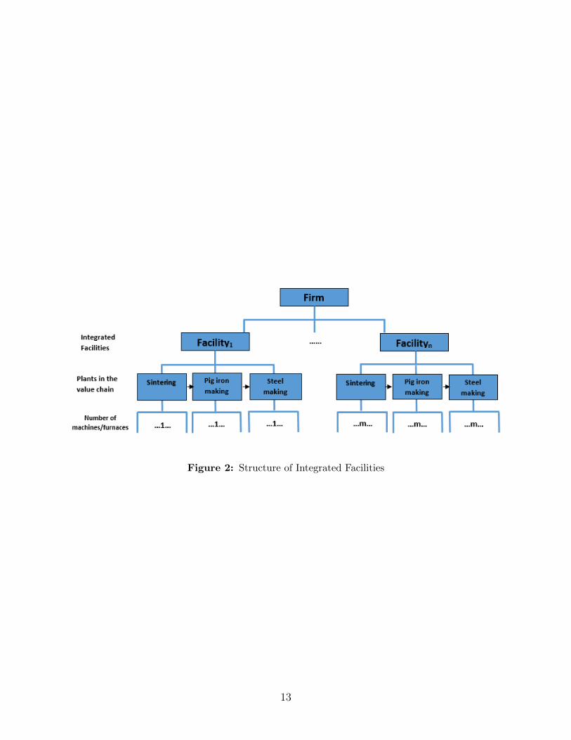
Figure 2: Structure of Integrated Facilities
13

or basic oxygen furnaces, respectively.
3.2.1 Ownership
We categorize firms by three basic types of ownership: central SOEs, provincial SOEs
and private firms. Central SOEs are under the direct supervision of the State-owned Assets
Supervision and Administration Commission (SASAC). We also define firms that have been
merged into central SOEs as central state-owned. Provincial SOEs are under the direction
of provincial or regional SASACs. Private firms in our sample include joint-ventures (JVs),
wholly owned foreign firms and privatized SOEs.29
Column (1) of Table 1 provides a breakdown of ownership for our sample, which is skewed
in favor of state-owned firms, at the equipment level by stage of production and by integrated
facility. In each of the three stages of production, between seventy and eighty percent of
machines/furnaces are state-owned. State-owned firms are also consistently the source of
eighty percent of total production, with the remainder coming from private firms. Within
the state sector, provincial SOEs have the largest market share. From a policy perspective,
central SOEs are strategically more important and the major beneficiaries of policy choices
at the national level.
3.2.2 Size
Steel firms span a wide range of sizes at both the equipment and integrated facility level.
By industry convention, we measure the size of a sintering machine by its e↵ective area; size
of a blast furnace by its e↵ective volume; and the size of basic oxygen furnace by its tonnage.
We define the size of an integrated facility as the total size of basic oxygen furnaces within
the facility. These size measures directly reflect production capacity.
Panels A to C of Table 1 provide summary data on equipment size for each stage of
29Privatized SOEs were the product of restructuring e↵orts in the state sector in the late 1990s and early
2000s.
14

production by ownership. A clear ranking emerges: On average, machines/furnaces of central
state-owned facilities are the largest, followed by those of provincial state-owned and then
private facilities. A typical private machine/furnace is only 60 percent of the size of a central
state-owned machine/furnace. The average size of a private pig-iron furnace, for example,
is 699 cubic meters compared to 1230 for a furnace of a central state-owned facility. Note
also in columns (4) and (5) the wide range of equipment sizes within each ownership group.
Panel D of Table 1 provides comparable information at the integrated facility level. Central
SOEs operate the largest facilities, which on average are more than twice as large as those
of the private facilities (301 tons versus 131 tons), and a third larger than the facilities of
provincial SOEs (301 tons versus 227 tons).
In Table 2, we break down integrated facilities into size quartiles and report for each
quartile the total number of facilities by ownership and their respective shares of total steel
production. Almost half of the facilities in central SOEs are in the largest size quartile: they
produce 14.1 percent of total steel, and make up the largest share of total production by
central state-owned facilities. The number of facilities of provincial SOEs is fairly evenly
distributed throughout the quartiles, but those in the largest size quartile play a dominant
role in total steel production. In sharp contrast with the state-owned facilities, only a single
private integrated facility lies in the largest size group. Most private facilities are smaller in
size than the sample median. In terms of the total production of private facilities however,
the integrated facilities in the third quartile are the most important, and produce 37 percent
of the steel by private facilities.
3.2.3 Internal Configuration of Integrated Facilities
As part of a single integrated facility, firms will typically operate multiple production
units, e.g. sintering machines, blast furnaces or basic oxygen furnaces, in each stage of
production. In Table 3 we report the average number of machines/furnaces and their average
size for each stage of production by ownership and facility size. As before, we break down
15

Table 1: Summary Statistics of Equipment and Facility Size by Ownership
Panel A: Sintering (Machine)
(1) (2) (3) (4) (5)Number Mean Std. Dev Min Max
Total 343 156 127 24 853Central 56 204 161 24 853Provincial 203 158 127 24 550Private 84 122 84 24 360
Panel B: Pig Iron Making (Blast Furnace)
(1) (2) (3) (4) (5)Number Mean Std. Dev Min Max
Total 490 1016 926 128 5500Central 92 1230 1046 200 4038Provincial 249 1127 1036 128 5500Private 149 699 460 179 2680
Panel C: Steel Making (Basic Oxygen Furnace)
(1) (2) (3) (4) (5)Number Mean Std. Dev Min Max
Total 342 95 62 12 300Central 68 123 66 30 260Provincial 209 93 63 12 300Private 65 72 39 30 180
Panel D: Integrated Facility
(1) (2) (3) (4) (5)Number Mean Std. Dev Min Max
Total 136 218 185 30 990Central 26 301 212 30 840Provincial 77 227 190 30 990Private 33 131 96 40 540
Notes: The size of a sintering machine is measured byits e↵ective areas in m2; the size of a blast furnace ismeasured by its e↵ective volume in m3; the size of abasic oxygen furnace is measured by its tonnage. Facilitysize is measured by the total size of basic oxygen furnaces(steel making) within the facility.
16

Table 2: Number and Production Share of Integrated Facilities by Size
Panel A: Size Distribution of Integrated Facilities
(1) (2) (3) (4) (5)1st quartile 2nd quartile 3rd quartile 4th quartile TotalNumber Number Number Number Number
Central 3 6 5 12 26Provincial 16 21 18 22 77Private 13 11 8 1 33Total 32 38 31 35 136
Panel B: Output Share by Integrated Facilities Size
(1) (2) (3) (4) (5)1st quartile 2nd quartile 3rd quartile 4th quartile Total
Output Share Output Share Output Share Output Share Output ShareCentral 1.1% 1.5% 2.9% 14.1% 19.5%Provincial 5.8% 11.6% 14.3% 30.9% 62.5%Private 4.3% 4.6% 6.7% 2.4% 18.0%Total 11.1% 17.6% 23.8% 47.5% 100.0%
Notes: Facility size is measured by the total size of basic oxygen furnaces (steel making) withinthe facility. The size of a basic oxygen furnace is measured by its tonnage. The size quartilesare calculated over the facility-month observations in the whole sample and are defined asfollows: <90, [90,160), [160,300) and �300. Output is measured in tons of steel.
17

integrated facilities into size quartiles. As a general rule, the number of machines/furnaces
used in each stage increases with the facility quartile. The increase however is less than pro-
portional to the increase in the facility size, implying an increase in average machine/furnace
size with the size of the integrated facility. For central state-owned facilities, the number
of sintering machines and blast furnaces actually falls with facility size. For steel, they in-
crease, but less rapidly than they do in either provincial state-owned or private facilities.
This behavior gives rise to systematic di↵erences in the number of machines/furnaces and
their size in each stage of production as the size of the integrated facility increases. In par-
ticular, central state-owned facilities consistently operate the smallest number and largest
machines/furnaces in each size category, followed by provincial state-owned and then private
facilities. Alternatively, when private firms build larger integrated facilities, they do so using
more machines/furnaces of smaller average size compared to SOEs.30
The Nature of Internal Configuration A firm’s choice with respect to the internal
configuration of their operations reflects both supply and demand side factors. In the Ap-
pendix, we sketch out an illustrative model that captures influences on the size and number
of equipment a firm operates and possible tradeo↵s. We abstract in the model from deci-
sions on total investment in production capacity, that is, we take investment in production
capacity as given.
Increasing returns to scale in equipment (furnace) size provide firms clear incentives to
achieve their desired production capacity using larger equipment (furnaces).31 As they try
to expand however, private firms face much more severe constraints compared to SOEs.
Foremost are central government regulations, which make it very di�cult for private sector
30To examine this relationship more fully, we estimate Poisson regressions of the number of equipment in
each stage of an integrated facility on log facility size and log size interacted with our ownership dummies
for each individual stage. We estimate related regressions for log equipment size on facility size, results of
which are reported in the Appendix.
31Estimates of return to scale are reported in Section 5.1.
18

firms to obtain the permission required to build larger facilities. These kinds of hurdles have
increased with problems of excess capacity in the industry. Firms often try to circumvent
these restrictions by carrying out a series of smaller projects that use smaller equipment
(furnaces).
Better human capital and higher quality raw materials are needed to take full advantage
of the new technology embodied in larger equipment (furnaces). Private sector firms are
disadvantaged vis-a-vis SOEs in both respects, thereby reducing the returns to installing
equipment (furnaces) of larger size.32 The same is true with respect to the cost of finance,
which makes it more di�cult for private firms to mobilize the funds needed to make the
investments associated with larger equipment (furnaces).
Demand-side considerations and profitability may also factor in, but in the opposite
direction. In the face of demand shocks, it is costly for firms to shut down (start up)
furnaces; moreover, these costs are increasing in the size of the equipment. This makes
it much more di�cult for a firm with a large furnace to adjust to demand shocks in the
short run. By contrast, firms with smaller units can adjust production more e�ciently by
simply suspending operations in a subset of their furnaces rather than by shutting down their
entire operations. In principle, this logic should apply equally to private firms and SOEs.
Di↵erences in the weight on profit maximization in the firm’s objectives however may make
such behavior more common in the case of private sector firms.
32Human capital and new technology associated with larger machines and furnaces are considered comple-
mentary to each other, a feature we discuss more in detail in Section 5.3. Firms choose the size of furnaces by
maximizing the discounted value of expected future profits, which depends on expected future environments
including the possibilities of accumulating human capital. Although private firms may be constrained by
human capital in the short-run, they may still have incentives to use equipment of larger size if they can
accumulate enough human capital over time to match with newer technology.
19

Table 3: Internal Configuration of Integrated Facilities by Size
Sintering (Machine)
(1) (2) (3) (4) (5)Ownership Variables Total 1st quartile 2nd quartile 3rd quartile 4th quartileCentral Number of Machines 1.98 1.89 2.38 2.50 1.63
Average Size 274 104 95 222 416Provincial Number of Machines 2.41 1.77 2.22 2.41 2.91
Average Size 186 117 141 225 236Private Number of Machines 2.12 1.71 2.31 2.09 5.00
Average Size 129 74 147 151 360
Iron Making (Blast Furnace)
(1) (2) (3) (4) (5)Ownership Variables Total 1st quartile 2nd quartile 3rd quartile 4th quartileCentral Number of Furnaces 2.32 2.48 2.28 2.13 2.38
Average Size 1938 435 985 1902 2768Provincial Number of Furnaces 2.66 1.99 2.84 2.59 2.90
Average Size 1423 633 809 1770 2145Private Number of Furnaces 2.82 1.85 3.29 3.56 3.00
Average Size 707 482 614 828 2680
Steel Making (Basic Oxygen Furnace)
(1) (2) (3) (4) (5)Ownership Variables Total 1st quartile 2nd quartile 3rd quartile 4th quartileCentral Number of Furnaces 2.44 1.37 1.83 2.26 3.08
Average Size 127 48 87 94 180Provincial Number of Furnaces 2.56 1.49 2.21 3.09 3.09
Average Size 94 46 67 81 152Private Number of Furnaces 1.90 1.09 2.00 2.69 3.00
Average Size 75 54 79 84 180
Notes: Facility size is measured by the total size of basic oxygen furnaces (steel making) within thefacility. The size quartiles are calculated over the facility-month observations in the whole sample andare defined as follows: <90, [90,160), [160,300) and �300. The size of a sintering machine is measuredby its e↵ective areas in m2; the size of a blast furnace is measured by its e↵ective volume in m3; thesize of a basic oxygen furnace is measured by its tonnage.
20

4 Estimating Total Factor Productivity of Integrated
Facilities
This section describes a framework for estimating total factor productivity of multiple-
stage production systems. Section 4.1 discusses the timeline of firms’ decision. Section
4.2 presents the theoretical framework and the methodology to construct productivity for
integrated facilities. Section 4.3 explains the details of our estimation procedure.
4.1 Description of Decision-Making
Firms make choices regarding investment and production. At the beginning of each
year, a firm observes its state, which includes observable variables that a↵ect their input
access, output market, and borrowing/regulatory constraints that depend on ownership.
Based on its initial state, the firm chooses its targeted level of total production to maximize
current profit. This production must then be allocated among integrated facilities and
machines/furnaces in each stage to minimize its total production cost. During the year, the
firm carries out the production plan and generates final outputs. At the end of the year, the
firm decides on investment, which depends on the current state. This decision has dynamic
implications: first, larger machines/furnaces are less flexible with respect to input choice and
potentially more costly to maintain/adjust, which a↵ects the expected payo↵ when there is
uncertainty in the input and output market; and second, larger machines/furnaces enjoy
the benefits of increasing returns to scale. Moreover, the choice of investment (i.e., the size
of the facility, and its internal configuration) may be limited by various constraints (e.g.
tighter regulatory hurdles, access to finance, human capital, raw materials, etc) that depend
on ownership.
Since we have a short panel, we leave the investigation of the full industry dynamics for
future research. This paper centers on productivity di↵erences by facility ownership related
to facilities’ internal configuration. Here we take advantage of the monthly frequency of
21

our data at the facility level and focus on the monthly production of facilities. At the
beginning of each month, each facility observes its stock of capital and labor and then the
productivity of its individual machines/furnaces. Based on these observables, the facility
decides intermediate inputs for its individual machines/furnaces. Note that the facility
obtains its intermediate inputs used in a downstream stage from production in the previous
stage. Following convention, we assume that intermediate input choices are monotone with
respect to productivity in each corresponding stage. At the end of this month, the facility
decides on the number of workers and maintaining/utilizing certain machines/furnaces in
the next month.
4.2 A Model of Multiple-Stage Production
In each period t, an integrated facility (facility “i”) engages in three major stages of
production, i.e., sintering (stage “1”), pig iron making (stage “2”) and steel making (stage
“3”). Along this production chain, output in each stage serves as the key material input
for the subsequent downstream production stage. Each stage (plant) may involve a single
or multiple machines/furnaces j. For simplicity, we omit i and t in the description of the
model.
A complete production process is described as below:
8>>>>>><
>>>>>>:
Y1j1 = min{e!1j1L↵11j1K
�11j1 , �1R1j1}e✏1j1 ,
Y2j2 = e!2j2+✏2j2L↵22j2K
�22j2R
�22j2 ,
Y3j3 = e!3j3+✏3j3L↵33j3K
�33j3R
�33j3 ,
(1)
22

where
X
j1
Y1j1 =X
j2
R2j2 ,
X
j2
Y2j2 =X
j3
R3j3 ,
Y3 =X
j3
Y3j3 ,
and R1j1 represents crude iron ore fine, Y1j1 and R2j2 denote sinter, Y2j2 and R3j3 pig iron,
and Y3j3 denotes the final product steel.33 Our measure of capital Ksjs is the capacity of
the equipment j in stage s, s = 1, 2, 3, and Lsjs is the corresponding number of employees.
Productivity !sjs is Hicks-neutral. Moreover, output from di↵erent machines/furnaces within
a stage are perfect substitutes. As sintering is an agglomeration process that reshapes iron
ore to the size and strength necessary for pig-iron making, this stage of production is assumed
Leontief in materials.34
Our model reflects several important properties of production in the steel industry. First,
inputs in di↵erent stages are not perfect substitutes, an assumption that is implicitly imposed
33Strictly speaking, iron ore fed into the furnace is a mixture of 75% sinter, 15% pellets and 10% lump
iron ore. Since we have limited information on the latter two, we abstract from their role in the first stage
and use total tonnage of the mixture in the second stage. Provided that the proportions are constant, this
simplification produces consistent estimates except for the intercept in the second-stage production function.
34Substitution may exist between raw iron ore and labor (capital), mostly likely due to the quality of
iron ore. However, we do not have information on the raw iron ore used in sintering. As we discuss more
fully below, our inability to control for raw material di↵erences likely results in a lower bound estimate of
productivity of private firms in sintering relative to SOEs. In pig iron making and steel making, taking furnace
size as given, a Leontief production function in materials may better describe the production technology
because materials are used in fixed proportions in the production process based on engineering designs.
However, the share of material inputs in production changes with furnace size, suggesting that a Leontief
production function in materials likely fails to capture the potential substitutability. We provide estimation
results using Leontief production functions in the Appendix.
23

in the standard firm-level production function. Second, upstream inputs, namely, labor and
capital, contribute to the entire production chain through their role as intermediate material
providers. Ignoring these features may result in biased estimates of input elasticity, and
thus, estimates of returns to scale and TFP.
To see this more clearly, consider as a counterpart to our production function process the
standard aggregate (log) production function for firm i at time t. We omit subscripts i and
t for simplicity.
y3 = ! + ↵l + �k + ✏,
where l is the logarithm of total labor input and equal to log(L1+L2+L3), and k is log(K1+
K2+ K3), the logarithm of total capital input measured in value terms. In the case of labor,
the aggregate production function implicitly assumes that the contribution of labor input
to output is of the form of (L1 + L2 + L3)↵, which implies that what matters to production
is the total amount of labor input and not the allocation of labor across production stages.
Labor inputs in each stage are perfectly substitutable with firms able to move workers freely
across stages at no expense of output. In contrast, our multi-stage specification allows
the role of labor to di↵er by stage. For example, the contribution of labor is of the form
of (L↵1�2�31 L↵2�3
2 L↵33 ) in the case in which each stage operates a single machine/furnace.
Moreover, the elasticity coe�cients are asymmetric, reflecting the sequential nature and
relative importance of these inputs.
Another advantage of the above production system is that it allows intuitive calculation
of facility-level return to scale and aggregation of stage productivity. First, we calculate the
facility-level return to scale, defined as the ratio between the percentage change in output
and the associated proportional change in inputs. Multiplying each capital and labor term
24

in production process (1) by a positive constant a leads to new amounts of outputs
8>>>>>><
>>>>>>:
Y1j1(a) = a↵1+�1Y1j1 ,
Y2j2(a) = a↵2+�2a(↵1+�1)�2Y2j2 ,
Y3j3(a) = a↵3+�3a[(↵2+�2)+(↵1+�1)�2]�3Y3j3 .
Note that a↵s+�s , where s = 1, 2, 3, is due to the proportional changes in the current stage
capital and labor. This proportional change propagates into the next stage and has a pro-
portional e↵ect on its output, as well. Therefore, the facility-level returns to scale (RS) is
characterized by the sum of the capital and labor elasticities in each stage of production
weighted by the material input elasticities:
RS = (↵1 + �1) · �2�3 + (↵2 + �2) · �3 + (↵3 + �3). (2)
The propagation e↵ects on the outputs in the downstream stage deserve some attention.
Outputs from the upstream stage are intermediate inputs in the immediate downstream
stage. In principle, the firm could change intermediate input use by di↵erent proportions in
downstream furnaces. However, due to the homogeneity of the production functions, it is
optimal for the firm to apply the same proportional change to each furnace.35
Second, we follow Domar (1961) to construct an estimate for facility-level productivity
by aggregating productivity across the three stages. In particular, we define facility-level
productivity as a weighted sum of stage productivity, i.e.,
! = !1 · �2�3 + !2 · �3 + !3. (3)
35This can be seen clearly by solving the following optimization problem. Rjs(a) =
arg maxRjs ,js=1,2,...,J
Pjs
e!jsK↵sjs
L�sjsR�s
jss.t.
Pjs
Rjs = a ⇤Pjs�1
Yjs�1 . Solving the above problem, we obtain
that Rjs(a) = a ⇤Rjs . A detailed proof is available in the Online Appendix.
25
We measure stage-level productivity !s by the weighted average productivity across ma-
chines/furnaces of stage s, s = 1, 2, 3, using the deterministic parts of the production func-
tion as weights. Intuitively, the facility-level productivity ! reflects the sum of productivity
in each stage of production weighted by its importance in the production chain using elastic-
ities. Alternatively, we can use the value shares of pig iron and sinter out of the total value
of steel as the corresponding weights.36
The facility-level productivity reflects how e�ciency variations in each stage propagate
into later stages. We now describe the intuition using the case in which each stage only
involves a single machine/furnace. Applying the Leontief first-order condition for sintering,
we proceed with the following (log) production system:
y3 = ! + ↵1�2�3l1 + ↵2�3l2 + ↵3l3 + �1�2�3k1 + �2�3k2 + �3k3 + ✏,
where ! ⌘ !3 + �3!2 + �2�3!1 and ✏ ⌘ ✏3 + �3✏2 + �2�3✏1 are facility-level productivity and
facility-level noise, respectively.
4.3 Estimation Approach
In this section, we develop a modified control function approach to estimate the pro-
duction system of vertically-integrated steel facilities. This approach is based on Olley and
Pakes (1996) and relies on a production unit’s choice on intermediate inputs to control for
unobserved productivity (Levinsohn and Petrin (2003)). A major advantage of our data is
that it contains equipment-level information on inputs and output, which allows estimating
production functions by stage-equipment and the calculation of equipment-level productivity
estimates.37
36The derivation of the alternative weights is described in the Appendix.
37We abstract from firms’ entry/exit decisions since they are not prominent in the data. We also do not
take into account monthly entry/exit decisions on machines/furnaces, but these could be dealt with in a man-
ner similar to Olley and Pakes (1996). E↵ectively, we can estimate the probability that a machine/furnace
26

We adapt the control function approach to allow for interdependence across stages within
the facility. To this end, we allow the optimal intermediate input demand function of a
machine/furnace to depend on not only its own state capital and labor, but also the amount
of production required in the subsequent stages of production. For simplicity, we omit
subscript i in the description of our approach. The demand functions of intermediate inputs
of the three production stages �st(·), s = 1, 2, 3, are as follows:
e1j1t = �1t(k1j1t, l1j1t,!1j1t, k2t, l2t, n2t,!2t, k3t, l3t, n3t,!3t), (4)
e2j2t = �2t(k2j2t, l2j2t,!2j2t, k3t, l3t, n3t,!3t), (5)
e3j3t = �3t(k3j3t, l3j3t,!3j3t), (6)
where kst,lst,!st are the average capital, labor and TFP of stage s, s = 2, 3, and nst the total
number of machines/furnaces of stage s. We use energy input to control for unobserved
TFP in sintering !1j1t and pig iron making !2j2t, and use scrap steel input to control for
unobserved TFP in steel making !3j3t.
Following Ackerberg et al. (2015), we assume that �st(·) is strictly monotone in !sjst
conditioning on (ksjst, lsjst), and for sintering and pig iron making, on the information of
downstream stages as well. In addition, the scalar unobservability condition also holds in
our setting due to the timing assumptions of firms’ input choices, so we can invert the above
relationships to control for the unobserved productivity. To proceed, we first invert the
demand function of steel making (6), estimate the production function of this stage, and
obtain estimates of average TFP b!3t. After we plug the estimated b!3t into the intermediate
input demand function for pig iron making, the only remaining unobservable in the demand
function (5) is productivity !2j2t. We then invert the demand function (5) to obtain a
control function for productivity !2jst and estimate the stage-2 production function. Next,
we plug both the estimated productivity of pig iron making b!2t and steel making b!3t into the
shuts down and use it as a control in our production function estimation.
27

intermediate input demand function of sintering (4) and estimate the production function
of sintering.
Equations (7), (8), and (9) provide the control functions for steel making, pig iron making
and sintering.
!3j3t = ��13t (k3j3t, l3j3t, e3j3t), (7)
!2jt = ��12t (k2j2t, l2j2t, e2j2t, k3t, l3t, b!3t), (8)
!1jt = ��11t (k1j1t, l1j1t, e1j1t, k2t, l2t, b!2t, k3t, l3t, b!3t). (9)
Our first-step estimating equation for each individual stage is then given by the equation
below, which expresses output y as a semiparametric function of (ksjst, lsjst, esjst, rsjst) and
of the information of downstream stages in the case of stage 1 sintering and stage 2 pig iron
making.
ysjst = ↵slsjst + �sksjst + �srsjst + ��1st (·) + ✏sjst.
As usual, we collect the deterministic terms and denote them as �st(·) ⌘ ↵slsjst + �sksjst +
�srsjst + ��1st (·). Note that for stage s = 1, the same analysis follows by leaving out r1j1t due
to the Leontief technology.
Ackerberg et al. (2015) argue that it may take longer to adjust capital and labor input use
optimally than intermediate inputs, which include materials and energy. Since our data are
on a monthly basis and include large SOEs that face significant hiring and firing costs, labor
is likely to be fixed or quasi-fixed. Therefore, it is reasonable to assume that the demand
for intermediate inputs depends on productivity and the predetermined capital and labor
input. The advantage of using energy inputs as control variables is two-fold: first, energy
input is measured in terms of standardized coal, which addresses the issue of potential bias
resulting from quality di↵erences in inputs; and second, using energy input for the control
function throughout the first two stages keeps our estimation consistent. We approximate
28

�st(·) by a high order polynomial and use OLS regression for estimation. We also include
ownership dummies (Downership), time dummies (Dt) and province dummies (Dprovince)
in the regression. In pig-iron making, we adjust material input r by the percentage of pure
ore content to control for quality variation. Basic oxygen furnaces (steel making) di↵er
significantly in the share of steel that goes through secondary refining. One of the major
goals of secondary refining is to remove impurities from the molten steel, so the intensity
of secondary refining potentially reflects the quality of pig iron used in steel making. To
control for input quality in steel making, we also include in the first stage a dummy to
capture whether furnaces carry out secondary refining (Dsecondsjst) and then the share of
steel that goes through secondary refining (secondsjst).
In the second step, we estimate the parameters ✓ ⌘ (↵, �, �) 2 ⇥ by GMM, which exploits
a Markov assumption on the TFP and the timing of input choices. ⇥ denotes the parameter
space. In particular, we assume that TFP of each equipment j in stage s follows a first-order
Markov process:
!sjst = g(!sjs,t�1) + ⇠sjst,
which says that the current productivity shock consists of an expected term predicted by
productivity at t� 1 (!sjs,t�1) plus a deviation from the expectation, often referred to as the
“innovation” component (⇠sjst). Note that !sjst is identified up to ✓ from the first step after
taking out measurement error and unanticipated shocks from output. We regress !sjst on a
linear function of !sjs,t�1 to obtain g(!sjs,t�1).38 Denote !sjst(✓) ⌘ c�st(·)� ↵lsjst � �ksjst �
�rsjst. For a given ✓, g(·) can be estimated and thus ⇠sjst (up to ✓) is obtained. The latter
38The results are robust to higher order polynomials.
29

is used to construct the moment conditions:
E[(⇠sjst(✓) + ✏sjst)
0
BBBBBBBBBB@
lsjs,t�1
lsjst
ksjst
rsjs,t�1
�sjs,t�1(ksjs,t�1, lsjs,t�1, rsjs,t�1)
1
CCCCCCCCCCA
] = 0.
Since the capital stock is a state variable at t, it should be orthogonal to the innovation
shock on productivity at t. We use current labor (lsjst) as an instrument for itself because
of its dynamic feature, and also include labor at t� 1 as an additional instrument. And we
use lagged material input rsjs,t�1 as an instrument for rsjst. As pointed out by Gandhi et al.
(2017), the use of ⇠sjst+ ✏sjst rather than ⇠sjst alone in the moment condition is more general.
We search over the parameter space ⇥ to find ↵, � and � that minimize the above moment
conditions.
We use the GMM procedure to identify separately production function coe�cients for
each individual stage s in a backward order as described above, s = 3, 2, 1. As is commonly
done, we also add firms’ age to the production function to control for potential systematic
di↵erences in technology resulting from the learning-by-doing process.39 In steel making, we
allow the status of secondary refining (Dsecondsjs,t�1) and the share of secondary refining
(secondsjs,t�1) to enter the productivity evolution process since secondary refining technology
may potentially impact the law of motion of productivity.
Compared with a commonly used aggregate revenue production function, our proce-
dure has several advantages. First, our setup properly captures the characteristics of the
vertically-integrated production chain. Second, the use of input and output in physical units
in our estimation helps eliminate price biases, and allows us to recover true productions
39Ideally we want to use a machine/furnace’s age to capture this process. Lacking this information, we
use the firm’s age.
30
coe�cients.40 Third, our GMM estimates correct for any endogeneity bias due to the poten-
tial relationship between input usage and unobserved productivity. Finally, disaggregated
information on inputs and output by stage of production allows us to estimate accurately a
multi-stage production system.
Measurement Errors The use of input and output measured in physical units helps avoid
potential biases introduced by heterogeneous prices, which could reflect for example market
power, misallocation, etc. But measures in physical terms can have flaws too, and may
not capture potential quality di↵erences in output, capital vintage, raw materials, or in the
facility’s human capital. The number of employees that we use to measure labor abstracts
from di↵erences in workers’ skill level. Similar issues arise in our use of equipment capacity
as our measure for the capital stock. In Section 6, we return to these issues and provide
several robustness checks for possible biases stemming from these sources.
5 Main Results
5.1 Production Function Coe�cients
Table 4 presents estimates of the production functions for sintering, iron making and steel
making, the three major production stages along the value chain for steel. For each stage of
production, we report results using both OLS and GMM. For sintering, the coe�cients are
only provided for labor and capital, and not for materials, reflecting the assumed Leontief
technology. The elasticities are largest for materials, followed by capital and labor. Of the
three stages, sintering is the most capital intensive, followed by pig-iron and steel making.
40For a detailed discussion of the biases encountered when using sales and expenditure data, see De Loecker
and Goldberg (2014).
31
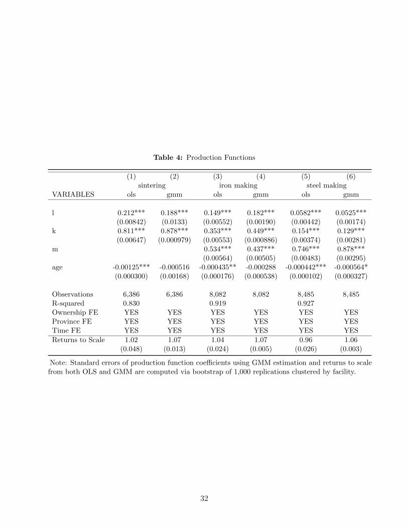
Table 4: Production Functions
(1) (2) (3) (4) (5) (6)sintering iron making steel making
VARIABLES ols gmm ols gmm ols gmm
l 0.212*** 0.188*** 0.149*** 0.182*** 0.0582*** 0.0525***(0.00842) (0.0133) (0.00552) (0.00190) (0.00442) (0.00174)
k 0.811*** 0.878*** 0.353*** 0.449*** 0.154*** 0.129***(0.00647) (0.000979) (0.00553) (0.000886) (0.00374) (0.00281)
m 0.534*** 0.437*** 0.746*** 0.878***(0.00564) (0.00505) (0.00483) (0.00295)
age -0.00125*** -0.000516 -0.000435** -0.000288 -0.000442*** -0.000564*(0.000300) (0.00168) (0.000176) (0.000538) (0.000102) (0.000327)
Observations 6,386 6,386 8,082 8,082 8,485 8,485R-squared 0.830 0.919 0.927Ownership FE YES YES YES YES YES YESProvince FE YES YES YES YES YES YESTime FE YES YES YES YES YES YESReturns to Scale 1.02 1.07 1.04 1.07 0.96 1.06
(0.048) (0.013) (0.024) (0.005) (0.026) (0.003)
Note: Standard errors of production function coe�cients using GMM estimation and returns to scalefrom both OLS and GMM are computed via bootstrap of 1,000 replications clustered by facility.
32

Weights for Returns to Scale and TFP Construction In order to construct facility-
level returns to scale, we need to integrate the sum of the capital and labor elasticities in
each stage of production weighted by the material input elasticities. For the construction of
facility-level TFP, we can use either the elasticity of material inputs in each stage or value
shares to integrate estimates of stage-level TFP into an aggregate measure of TFP at facility
level. In Table 5 we report the two sets of weights for each stage of production. As we move
downstream, the contribution of stage-level production to facility-level returns to scale and
e�ciency increases: The weight on sintering is 0.38 compared to weights of 0.88 and 1.0 on
iron-making and steel production, respectively. Our two sets of weights are also fairly similar
in magnitude and deliver similar estimates of TFP. The subsequent analysis is based on the
TFP estimates weighted by the elasticities.
Returns to Scale Our OLS estimates suggest increasing returns to scale in sintering (1.02)
and iron making (1.04), and decreasing returns to scale in steel making (0.96). In contrast,
our GMM estimates imply increasing returns to scale in each stage of production.41 The
sum of the input elasticity is slightly larger for sintering (1.07) and iron making (1.07) than
for steel making (1.06). These di↵erences are reflected at the facility level (see equation
(2) in section 4.2), where we find increasing returns to scale of 1.14 based on the GMM
estimates, and 0.99 using the OLS estimates.42 At the facility-level, the OLS estimates
suggest slight decreasing returns to scale due to the fact that the final stage production
o↵sets the advantages of increasing returns to scale in the first two stages. In contrast,
the facility-level estimate from GMM is larger than the returns to scale in the individual
41We replicate the OLS and GMM estimation for steel making for a thousand bootstrapped samples, and
find that the mean of the returns to scale from GMM is statistically larger than the returns to scale from the
OLS. The di↵erence between OLS and GMM for sintering and pig iron making is not statistically significant,
however both sets of estimates imply increasing returns to scale.
42The standard error for the estimate of the returns to scale calculated from the GMM estimates at the
facility level is 0.008.
33

stages, suggesting that the three stages contribute to overall increasing returns in a mutually
reinforcing way. Therefore, the OLS estimates can lead to misleading conclusions about the
features of steel technology. Our facility-level estimate based on the GMM procedure is
also larger than several recent estimates for the industry, notably, an estimate of 1.03 by
Collard-Wexler and De Loecker (2015) for the US, and 1.07 for China by Sheng and Song
(2012).43 The increasing returns to scale at both the equipment- and facility-level provide
incentives for steel firms to build larger facilities and install larger machines/furnaces to take
advantage of falling long-run average costs.
5.2 Productivity Di↵erences in Integrated Facilities
5.2.1 Productivity Di↵erences by Ownership
We present estimates of facility-level productivity di↵erentials by ownership in Table 6.
Column (1) shows that private integrated facilities are on average 7.4 percent more productive
than the facilities in central SOEs, and are 1.1 percent more productive relative to provincial
SOEs. The magnitude of the private ownership premium in steel is small by comparison with
Hsieh and Song (2015)’s recent estimate of 33 percent for 2007 for the manufacturing sector,
but more in line with Berkowitz et al. (2017), who find an average 8.2 percent productivity
premium of private firms relative to SOEs between 2003 and 2007.44 With value added in
43Possibly underlying these di↵erences is some combination of the estimation of an aggregate production
function, and in the case of Sheng and Song (2012), estimation of a revenue production function. The latter
is necessary because of the lack of firm-level price information. De Loecker and Goldberg (2014) point out
that variation in both output and input prices in a revenue production function likely results in a downward
bias in production function coe�cients and therefore a lower returns to scale. Collard-Wexler and De Loecker
(2015) construct firm-level input and output deflators, and thus e↵ectively estimate a production function
in physical terms.
44Di↵erences in these estimates may come from several sources: First, estimation of a value-added versus
gross-output production function. Although both value-added and gross-output based TFP indices provide a
measure of technological change, the two will not necessarily be the same (Balk (2009)). Second, di↵erences in
34

Table 5: Weights for Returns to Scale and TFP Aggregation
(1) (2) (3)Weight 1 Weight 2Elasticity Value Share
Sintering �2 ⇤ �3 Mean Std Dev0.38 0.52 0.16
Iron making �3 Mean Std Dev0.88 0.82 0.05
Steel making 1 1
Notes: �2 is the estimated elasticity of materialinput (iron ore) in iron-making production func-tion. �3 is the estimated elasticity of materialinput (iron) in steel-making production function.
assumptions relating to the underlying production technology, e.g., Cobb-Douglas versus CES versus translog,
may result in di↵erences in estimated TFP and our productivity ranking. And third, some estimates may
only reflect within-sector variation, while others capture both within and between sector di↵erences in TFP.
35

the steel sector 25-30 percent of gross output, even modest productivity di↵erences of the
sort we estimate translate into significant di↵erences in profitability by ownership, which
have wider implications.
5.2.2 The Larger, the Better?
We documented systematic di↵erences in the size of integrated facilities by ownership:
SOEs in general operate much larger facilities. The scatter plot of TFP against facility size in
Figure 3 demonstrates a slight negative relationship between the two for the full sample and
a more pronounced negative relationship for private facilities. To examine this relationship
more systematically, we add facility size to the regression of TFP on firm ownership, and
also run regressions on facility size that include interaction terms of ownership dummies
with facility size. Estimates are provided in Table 6 columns (2) and (3), and confirm the
results of Figure 3. On average, TFP falls with facility size, as indicated by column (2)
of Table 6. The productivity premium of private facilities relative to facilities of central
SOEs also drops by almost half, to 3.8 percent. Moreover, private facilities now become 1.1
percent less productive than provincial state-owned facilities. Examining the size e↵ect by
ownership, we see that size appears to have a small positive e↵ect on TFP for central state-
owned facilities. In sharp contrast, for private firms, and slightly less so for provincial SOEs,
productivity of integrated facilities declines with size. The coe�cient on the interaction
term for private facilities implies that with a doubling in size, their productivity declines
by 14.7 percent relative to central state-owned facilities. This has the e↵ect of reducing the
productivity premium of these facilities relative to central state-owned facilities at larger
sizes. When facility size is above the median, TFP of private facilities falls below that
of central state-owned facilities. We observe the same pattern in the comparison between
private and provincial state-owned facilities.
36

Table
6:ProductivityDi↵eren
cesby
Ownership
andSize
(1)
(2)
(3)
(4)
(5)
(6)
(7)
(8)
(9)
(10)
(11)
(12)
Facility
Facility
Facility
Sintering
Sintering
Sintering
Iron
Iron
Iron
Steel
Steel
Steel
Mak
ing
Mak
ing
Mak
ing
Mak
ing
Mak
ing
Mak
ing
Variables
logtfp
logtfp
logtfp
logtfp
logtfp
logtfp
logtfp
logtfp
logtfp
logtfp
logtfp
logtfp
logsize
-0.047
90.04
34-0.090
3***
-0.118
***
-0.033
8***
-0.034
6-0.052
9***
-0.021
2(0.031
9)(0.046
7)(0.023
2)(0.033
9)(0.008
49)(0.022
8)(0.005
85)
(0.015
1)PrivateXlogsize
-0.147
-0.022
5-0.055
2-0.067
9**
(0.093
3)(0.066
3)(0.034
9)(0.032
9)ProvincialXlogsize
-0.108
*0.05
040.01
16-0.032
7**
(0.063
3)(0.045
9)(0.024
5)(0.016
2)Private
0.07
430.03
820.80
2*-0.108
**-0.144
***
-0.051
20.06
12**
*0.04
29*
0.39
3*0.06
15**
*0.03
16**
0.33
1**
(0.063
1)(0.072
8)(0.462
)(0.051
8)(0.048
5)(0.318
)(0.020
7)(0.022
1)(0.235
)(0.015
2)(0.015
6)(0.138
)Provincial
0.06
330.04
900.63
3*-0.093
0**
-0.115
***
-0.360
0.02
220.01
58-0.062
20.01
55-0.006
300.14
7*(0.051
6)(0.054
3)(0.360
)(0.044
6)(0.040
8)(0.231
)(0.019
4)(0.019
6)(0.176
)(0.009
47)
(0.009
93)
(0.079
1)Con
stan
t-0.113
**0.14
1-0.357
0.03
420.47
1***
0.60
8***
-0.084
2***
0.14
6**
0.15
1-0.042
0***
0.20
4***
0.05
44(0.048
1)(0.187
)(0.273
)(0.037
2)(0.113
)(0.165
)(0.021
8)(0.065
1)(0.165
)(0.008
74)
(0.029
9)(0.074
9)
Observations
3,44
03,44
03,44
08,72
88,72
88,72
811
,836
11,836
11,836
8,51
08,51
08,51
0R-squ
ared
0.02
20.03
60.05
10.01
50.04
30.04
60.02
00.03
30.03
80.04
80.15
10.16
2Tim
eFE
YES
YES
YES
YES
YES
YES
YES
YES
YES
YES
YES
YES
Notes:Central
state-ow
ned
facilities
andtheirmachines/furnaces
aretheom
ittedgrou
p.Private
andprovincial
indicateow
nership
dummies.
Thesize
ofasinteringmachineismeasuredby
itse↵
ective
areasin
m2;thesize
ofablast
furnaceismeasuredby
itse↵
ective
volumein
m3;
thesize
ofabasicoxyg
enfurnaceismeasuredby
itstonnag
e.Facilitysize
ismeasuredby
thetotalsize
ofbasicoxyg
enfurnaces
(steelmak
ing)
within
thefacility.Standarderrors
areclustered
bymachines/furnaces
forstag
e-levelan
alysis
andby
facility
forfacility-level
analysis,but
not
correctedforthesamplingerrorin
constructed
productivity.
37

Figure 3: Facility-level TFP and Size of Integrated Facilities
Notes: By industry convention, facility size is measured by the total size of basic oxygen furnaces(steel making) within the facility; the size of a basic oxygen furnace is measured by its tonnage.Each plot represents a facility-month observation.
38
5.3 Productivity Di↵erences: A Further Look
This section takes advantages of our unique data to rationalize the productivity dif-
ferences that we identified above. Our analysis centers on two key questions: Where in
production is the premium coming from? Why does TFP decline with size for private firms
in particular?
Productivity Di↵erences by Stage of Production To examine the sources of the
observed productivity di↵erences, we first study the e↵ect of ownership on equipment-level
productivity. In columns (4), (7) and (10) of Table 6, we report estimates of productivity by
ownership for each stage of production. Estimates are obtained from simple OLS regressions
of the log of equipment-level TFP on ownership dummies that control for the e↵ect of
seasonality with the use of monthly dummies. In columns (5), (8) and (11), we report
results that also control for the size of equipment. In these regressions, equipment of central
state-owned facilities are our omitted category. In both pig-iron making and steel-making,
private facilities have a productivity advantage over central state-owned facilities of 6.1
percent and 6.2 percent, respectively. The premium of private facilities in both stages is
slightly smaller in comparison with provincial state-owned facilities. In sharp contrast, the
productivity ordering by ownership is reversed for sintering: Sintering machines of central
state-owned facilities are 10.8 percent more productive than private facilities, and 9.3 percent
more productive than provincial state-owned facilities. Clearly, the ordering of productivity
by ownership at the facility level follows that found in pig-iron making and steel making.
This implies that the sizeable productivity disadvantage of private facilities in sintering is
more than o↵set by their superiority in the two downstream stages of production.
What might help to explain the reversal in the productivity ranking in the case of sin-
tering? A regular supply of iron ore is critical to the running of sintering machines. SOEs,
especially central SOEs, typically enjoy privileged access to iron ore.45 Central SOEs source
45Interview with a steel consultant at Shanghai Securities Research Institute in December, 2014.
39
imported iron ore through long-term contracts directly with the importers, which enable
them to build up inventories of iron ore when prices are relatively low. In principle, sourcing
di�culties might force private facilities to operate their sintering machines at lower rates of
capacity utilization, which then show up as lower productivity. Data on capacity utilization
however reveal only modest di↵erences by ownership in the case of sintering.46 Nonetheless,
private facilities’ use of lower quality iron ore might hold the key to the di↵erences we observe
in productivity in sintering.47
In general, domestic iron ore is of much lower quality than imported ore and contains a
higher proportion of impurities.48 This is reflected, for example, in the silica content of the
iron ore, a chemical substance that lowers the quality of sinter and also adversely a↵ects the
production process. For domestic iron ore, the silica content ranges from 6.5 to 12 percent.
By contrast, imported iron ore is more homogeneous in pure ore content, and contains only
4 percent silica.49 Over the three-year period between 2009 and 2011, steel firms of all
ownership in China relied heavily on imported ore, however private firms used two-thirds
more domestic iron ore than did SOEs: 33.3 percent versus 20 percent.50 Data for 2010 and
2011 indicate that rich ore fines - a measure of the quality of crude ore used in sintering -
make up 60.1 percent and 62.8 percent of total crude iron ore processed in central SOEs in
these two respective years, compared to 47.5 and 46.2 percent in private firms, a di↵erence
of 12.6 and 16.6 percentage points, respectively.
46Capacity utilization is measured here as the ratio of operating days to total calendar days minus
scheduled maintenance days. Private facilities actually operate slightly more intensively than central state-
owned facilities by 1.8 percentage points.
47Factors influencing sintering process. July 8, 2013. http://ispatguru.com/factors-influencing-sintering-
process/
48See Gao (2006) for more details.
49The information on iron ore fines is based on data in Yu (2004).
50Data on iron ore are reported on an annual basis and cover two-thirds of the firms in the production
data.
40

Sintering is positioned at the very beginning of the value chain and entails the production
of high quality burden out of crude iron ore fines. The use of lower grade domestic iron ores
by private facilities necessitates additional processing in order to produce the iron ore of the
desired quality for pig-iron production. This ties up the processing equipment longer and
requires additional labor inputs, both of which translate directly into the lower equipment
productivity we observe.51 Depending on the substitution possibilities between labor, capital
and iron ore quality, inclusion of iron ore in the production function would likely reduce the
premium of SOEs over private firms in TFP in sintering.
Productivity Di↵erences and Internal Configuration As discussed in Section 3.2.3,
when private firms build facilities with larger capacity, they install larger machines/furnaces,
but more of them and of lower average machine/furnace size compared to SOEs. This
di↵erence is especially sharp as the size of integrated facilities grows larger, e.g., in the third-
quartile for pig iron making. This pattern may help explain the falling productivity premium
of private integrated facilities.
To identify the role of larger equipment size in explaining productivity di↵erences by
ownership, we add to the previous regressions an interaction term between equipment size
and our ownership dummies.52 The reported estimates in Table 6 suggest that equipment-
level TFP declines with equipment size. Moreover, equipment-level TFP in private facilities
declines relative to state-owned facilities as equipment size expands in all three production
stages, with the e↵ect more pronounced in pig-iron and steel making.
Several channels help to explain the above observation. First, larger furnaces and sinter-
ing machines utilize newer technologies, which firms only master with experience. Zhu et al.
51In iron- and steel-making, however, our production function estimation already factors in the quality
of the key material inputs. In fact, controlling for input quality changes only slightly the magnitudes of
productivity di↵erentials.
52Note that in these regression we may be picking up the systematic (and unobserved) correlation between
the size of the equipment and overall number of equipment the firm is running.
41

(2010) document that large furnaces fail to achieve their expected production e�ciency when
they initially go into operation because of firms’ limited technological capabilities. Firms
such as Baosteel, widely regarded as China’s most advanced steelmaker, invest heavily in
R&D, human resources, etc, to better align the firms’ technological capability with these
new technologies. Li (2011) and Yang et al. (2011) discuss the learning-by-doing e↵ects in
pig iron making for Baosteel and in steel making for Masteel, respectively. The decline in
TFP with equipment size in all ownership categories likely reflects less experience associated
with newer technologies.53 Later adoption of newer technologies by private firms, in turn,
may help explain the sharper decline in TFP with furnace size for these firms.
Second, larger furnaces and sintering machines require better human capital both on the
shop floor and in management, exactly the areas in which private firms face constraints.
Ahlbrandt et al. (1996) argue in the context of the US steel industry that for any given
level of technology, the best performing plants are those with the most capable production
workers. More generally, new technology and human capital are highly complementary.54 Li
(2011) points out, for example, that by design larger blast furnaces are more advanced in
their technology (e.g. energy saving and environmental friendly), and also more demanding
in the role of advanced management systems.55 In larger furnaces, workers must also control
the size, shape and temperature of the burdens fed into furnaces within much finer tolerances,
thereby putting a premium on higher quality shop-floor workers.56 Large furnaces also require
53However, our short panel cannot e↵ectively show such learning-by-doing e↵ect.
54Giorcelli (2019) finds that management and new machines were complementary using data on Italian
firms in the context of Productivity Program, a part of Marshall Plan.
55Larger blast furnaces require managers to adopt modern management procedures, such as “PDCA”, i.e.
Plan, Do, Check and Action. As large blast furnaces also generate huge amounts of data, management and
analysis of data are critical for operating and control of large and modern blast furnace. See “High Capacity
Iron Making with Large, Modern Blast Furnaces”, International Conference on Emerging Trends in Metals
& Minerals Sector. New Delhi, 5 September 2014.
56In addition, in larger furnaces, the production process must be more carefully monitored to ensure that
42

additional care and maintenance: A temporary breakdown lasting a single minute can result
in substantial costs.
Much lower levels of human capital in private facilities may contribute to the more rapid
drop-o↵ in TFP as equipment size rises.57 A growing literature documents the e↵ect of
ownership on a firms’ ability to access resources and capital. Drawing on a sample of private
enterprises in China, Garnaut et al. (2012) argue that private firms are not only financially
constrained, but are also constrained with respect to human capital.58 Iskandar (2015) uses
the World Bank 2012 survey data to provide evidence that private firms are constrained in
their ability to hire skilled and trained labor. The steel industry is no exception. In China’s
steel sector 18.7 percent of SOE employees had a college degree or higher compared to only
7.2 percent in private firms. The percentage of skilled labor in SOEs was almost two and a
half times higher than in private firms (4.7 versus 2 percent).59
Larger sintering machines and furnaces embody newer technologies that are highly com-
plementary with the human capital endowments of SOEs, e.g. more talented and experienced
managers and more highly skilled workers. Smaller machines and furnaces using earlier vin-
tage technologies are much less demanding in this regard, and thus more compatible with
the managerial talent, organizational capabilities and skill sets of private firms. Lower levels
slag is removed almost immediately because of the greater risk that it might clog the furnace as pressure
inside the furnace increases (Yao (2014)).
57In our regressions, we are not able to control for human capital di↵erences. Since human capital in
private firms is lower than SOEs, including human capital would likely raise the TFP premium of private
firms. The e↵ect of the size premium by ownership depends on the ratio of human capital in SOEs to private
firms by furnace size, which we do not have information on.
58The four surveyed cities include Beijing, Chengdu, Chengde and Wenzhou.
59The figures are based on the authors’ calculation using the 2004 Industrial Survey Data. We define
high skilled labor as the total number of technicians and high-skilled workers. Several studies have also
shown that state-owned firms in China have deep human resource reserves (e.g. Peng and Heath (1996);
Tan (2003)).
43

of human capital in private firms likely increase the time needed to digest and fully ex-
ploit the potential of new technology. Further, the greater number of machines/furnaces at
larger private facilities spreads scarce managerial resources even thinner, thereby lowering
the productivity of these private facilities.
6 Discussion
This section examines how measurement errors in capital and output might a↵ect our
main analysis.
6.1 Measurement Error in Capital
The use of production capacity as our measure of firm capital has its advantages, but
may still not fully capture di↵erences in capital intensity between firms.60 For example,
investment costs per unit of capacity, which we assume are constant, might increase with
equipment size.61 The potential bias results from two sources. First, the positive correlation
between capacity and unit investment cost leads to an upward bias in capital coe�cients.
Second, estimated productivity contains the unit price of capacity. Other things equal, the
overestimate of the capital stock in private facilities would lead to a downward bias in the
productivity di↵erentials that we found in pig-iron and steel making.
To see this more clearly, we express production as a function of price-adjusted capital k⇤,
where k⇤ is the product of capacity k, our capital measure in the baseline estimation, and
60One shortcoming of capital stock measures in value terms is that they include investments in pollution
abatement equipment, which are not separately identified in the data. While these investments are good
for the environment, they do not likely augment productivity. Firms that invest more in pollution control,
all else equal, will likely have lower TFP. The use of capital measures in physical (capacity) terms is not
susceptible to these biases.
61We extract the information on investment costs of steel plants by size from an internal report prepared
by the Chinese Metallurgy Planning Institute in August 2016 per the authors’ request.
44

the unit capacity price, p.
yi = ↵li + �k⇤i + �ri + !i + ✏i
= ↵li + �ki + �ri + �pi + !i + ✏i
In our baseline model, we treat unit capacity price p as measurement error, so our estimated
productivity is equal to �pi + !i. Since unit capacity price p is positively correlated with
capacity k, this leads to a potential upward bias in the estimated parameter on capital �.
Our estimates of productivity ownership di↵erentials are also likely to be biased because our
measure of productivity (�pi + !i) includes the unobserved unit capacity price. Consider
the estimated productivity di↵erential between private and central state-owned facilities, i.e.,
�(pprivatei �pcentrali )+(!privatei �!central
i ). The first term reflects capacity price di↵erences, and
the second measures the true di↵erence in productivity. As private facilities systematically
operate smaller equipment than central state-owned facilities, the unit capacity price of
private machines/furnaces is generally lower. Consequently, the first term of the productivity
di↵erential is negative, which gives rise to a downward bias in the estimated productivity
premium of private firms at the equipment level compared to central state-owned facilities.
We use the price information on investment of basic oxygen furnaces (steel making) to
adjust capital in this particular stage of production, and re-estimate the production function
for steel making using this adjusted capital measure. The estimated coe�cients are reported
in Table 7. Compared to the baseline estimation, using the adjusted capital generates a lower
coe�cient for capital, as predicted. We report the corresponding productivity di↵erentials
in Table 8. The productivity premium of private furnaces over central state-owned furnaces
rises slightly from 6.2 percent to 6.4 percent when we base our estimates on the price-adjusted
capital.
45

Table 7: Production Function: Robustness Check
(1) (2)
Steel MakingNon-Adjusted Price-Adjusted
Variables GMM GMM
l 0.0525*** 0.0520***(0.00174) (0.00174)
k 0.129*** 0.0920***(0.00281) (0.00258)
m 0.878*** 0.885***(0.00295) (0.00252)
age -0.000564* -0.000582*(0.000327) (0.000339)
Observations 8,514 8,514Ownership FE YES YESProvince FE YES YESTime FE YES YES
Note: Standard errors of GMM estimation arecomputed via bootstrap of 1,000 replications clus-tered by facility.
46

Table 8: Ownership Premium of Productivity in Steel Making: Robustness Check
(1) (2)
Non-Adjusted Price-AdjustedVariables logtfp logtfp
Private 0.0615*** 0.0641***(0.0152) (0.0153)
Provincial 0.0155 0.0147(0.00947) (0.00937)
Constant -0.0420*** -0.0413***(0.00874) (0.00861)
Observations 8,510 8,510R-squared 0.048 0.052Time FE YES YES
Notes: Furnaces of central state-owned facilitiesare the omitted group. Provincial and privateare ownership dummies. Standard errors are clus-tered by furnace.
47

Independent of furnace size, systematic di↵erences may also exist in the costs per unit
of capacity between private and state-owned facilities. In general, we expect private firms
to be more cost sensitive, and for them to be successful in finding ways to build furnaces of
any size at lower cost, and thus enjoy lower per unit cost of capacity relative to SOEs. This
source of measurement error would further underestimate productivity premiums of private
facilities. Similar to our discussion about the bias generated by ignoring the increasing unit
cost of capacity with equipment size, there will be an e↵ect coming through our estimate
of the elasticity for capital, and our estimate of the capital stock of these private facilities.
Additional information on capacity cost by ownership is needed to estimate the magnitude
of this bias.
6.2 Measurement Error in Output
In our data, output is measured in physical units, obscuring output quality di↵erences
between facilities. In principle, this could bias our productivity comparisons. Let y⇤ measure
quality-adjusted output, defined as a function of observed output y and X, a vector of output
quality measures. f is a general production function and is stage-specific but time-invariant.
y⇤i (yi, Xi) = f(li, ki, ri) + !i + ✏i (10)
Assuming that y and the quality components are additively separable
y⇤i = yi + �(Xi) (11)
Substituting equation (11) into equation (10), we obtain our baseline production function.
yi = f(li, ki, ri) + (!i � �(Xi)) + ✏i (12)
This makes explicit that estimated productivity ˆ!i � �(Xi) also incorporates output quality.
48

Table 9: Output Quality Di↵erences by Ownership
(1) (2) (3)
Sintering Iron Making Steel MakingVariables Grade Stability Premium Grade Secondary
Private -10.56** 1.354 -39.54***(4.243) (3.935) (7.873)
Provincial -2.481 -5.717 -26.77***(1.929) (3.689) (6.698)
Constant 90.79*** 65.92*** 56.25***(1.716) (3.365) (6.113)
Observations 8,728 11,836 8,510R-squared 0.027 0.018 0.093Time FE YES YES YES
Notes: All quality measures are in percentage points. Secondarydenotes the share of steel that goes through secondary steel refiningand provides an important piece of evidence on the quality of steel.Standard errors are clustered by machines/furnaces.
49

Table 10: Quality-Adjusted Ownership Premium of Facility-level Productivity
(1) (2) (3) (4) (5) (6)
Variables logtfp logtfp logtfp logtfp logtfp logtfp
logsize -0.0479 -0.0687** 0.0434 0.0238(0.0319) (0.0317) (0.0467) (0.0509)
PrivateXlogsize -0.147 -0.137(0.0933) (0.0901)
ProvincialXlogsize -0.108* -0.110*(0.0633) (0.0641)
Private 0.0743 0.0847 0.0382 0.0530 0.802* 0.765*(0.0631) (0.0665) (0.0728) (0.0712) (0.462) (0.449)
Provincial 0.0633 0.0724 0.0490 0.0652 0.633* 0.660*(0.0516) (0.0512) (0.0543) (0.0537) (0.360) (0.365)
Constant -0.113** -0.0478 0.141 0.257 -0.357 -0.237(0.0481) (0.111) (0.187) (0.201) (0.273) (0.287)
Observations 3,440 3,440 3,440 3,440 3,440 3,440R-squared 0.022 0.027 0.036 0.049 0.051 0.063sinter quality NO YES NO YES NO YESiron quality NO YES NO YES NO YESsteel quality NO YES NO YES NO YESTime FE YES YES YES YES YES YES
Notes: Central state-owned facilities are the omitted group. Provincial and privateare ownership dummies. Standard errors are clustered by facility.
50

Table 9 reports output quality comparisons across ownership: On average, private firms
produce lower quality sinter and steel but higher shares of premium grade pig iron compared
to SOEs.62
To see how these di↵erences in output quality a↵ect productivity di↵erentials by own-
ership, we re-estimate the facility-level productivity di↵erentials by adding as controls the
quality measure of each output. Table 10 shows that the productivity premium of private
facilities relative to central state-owned facilities increases slightly from 7.4 percent to 8.5
percent once we control for output quality. On the other hand, the premium relative to
provincial state-owned facilities remains more or less the same. In short, the premium of
private firms cannot be attributed to quality di↵erences in the output they produce.
7 Conclusion
This paper is one of the first to study the underlying sources of productivity di↵erences
by firms’ ownership structure through the lens of firms’ internal configuration. The new data
set that we construct provides equipment-level information on inputs and output in physical
units for each stage in the value chain of vertically-integrated facilities. We find that private
integrated facilities are on average 7.4 percent more productive than central state-owned
facilities, and 1.1 percent relative to provincial state-owned facilities. This ranking lines up
with our productivity estimates in the two downstream production stages, but central state-
owned facilities outperform in sintering, most likely because of their use of higher quality
raw materials. Back of the envelope calculations suggest that eliminating the premium of
central state-owned facilities in sintering would raise the premium of private facilities at the
facility level by an additional 4.1 percentage points, or to 11.5 percent overall.
62We have information on the stability rates of sinter and shares of premium iron, important qual-
ity measures of sinter and pig iron. Shares of secondary steel making provide evidence on the quality of
steel. Steel mills carry out secondary refining to produce higher quality steel. See detailed description at
https://www.steel.org/⇠/media/Files/AISI/Making%20Steel/Article%20Files/learning 2ndrefining.pdf
51

Table 11: Productivity Di↵erences by Ownership: Privatization
(1) (2) (3) (4)
Facility Sintering Iron Making Steel MakingVariables logtfp logtfp logtfp logtfp
Privatized 0.141* 0.0281 0.0739*** 0.0948***(0.0799) (0.0643) (0.0255) (0.0155)
New private 0.0307 -0.241*** 0.0514** 0.0365*(0.0741) (0.0550) (0.0220) (0.0208)
Provincial 0.0633 -0.0930** 0.0222 0.0156(0.0516) (0.0446) (0.0194) (0.00947)
Constant -0.113** 0.0333 -0.0843*** -0.0419***(0.0481) (0.0372) (0.0218) (0.00874)
Observations 3,440 8,728 11,836 8,510R-squared 0.029 0.037 0.021 0.063Time FE YES YES YES YES
Notes: Central state-owned facilities and their machines/furnaces arethe omitted group. New private, privatized and provincial are own-ership dummies. Standard errors are clustered by facility for facility-level analysis and by machines/furnaces for stage-level analysis.
52

We also find that the productivity premium of private facilities declines with facility
size, and actually turns negative for vertically-integrated facilities larger than the medium.
Some of the decline in the productivity premium of private facilities with size may arise from
less experience with newer technologies. This behavior also likely reflects choices of private
firms when they decide to build larger integrated facilities, most notably, the fact that they
install a larger number of smaller units, i.e. sintering equipment and furnaces, to achieve the
desired level of capacity. In this paper we suggest a number of constraints responsible for
these choices, which spreads their scarce human resources more thinly over a larger number
of units, and lowers their relative productivity. Our analysis suggests that the productivity
advantage of private facilities would be significantly higher if the constraints were removed.
Support for this conjecture comes in the form of the estimated premium of privatized
SOEs for whom constraints are less binding. A product of ownership reforms between the
late 1990s and 2005, privatized SOEs operate 13 out of the 33 private integrated facilities and
are the source of one-third of the steel production of private firms, or 7 percent of the total
steel production. We divide private firms into privatized SOEs and new private firms and
re-estimate productivity di↵erentials, which we report in Table 11. We observe pronounced
di↵erences, and at the facility level privatized SOES are 14.1 percent more productive than
central SOEs and 7.8 percent more than provincial SOEs. Much of the premium enjoyed by
private firms is a product of the superiority of privatized SOEs. Privatized SOEs outperform
other firms in all individual stages, including in sintering in which an average private firm
has enormous disadvantage compared to central SOEs.
These results are important in two important respects. First, they suggest that privatized
SOEs are likely less constrained than newly established private firms. Privatized SOEs, for
example, may be able to leverage the network of the former SOEs to help access key raw
materials, finance as well as human capital. Second, these results imply that private firms
would perform even better than SOEs if they were less constrained. Our earlier estimates
likely represent a lower bound of the return to changes that would put private firms on an
53

equal footing with SOEs.
Finally, in this paper we have focused largely on the constraints facing private firms in
their choice of plant size. As discussed in the end of Section 5.3, there are also advantages to
having a portfolio of plants with smaller average size. In order to examine these trade-o↵s
more carefully, we need to build and estimate a structural dynamic model that looks at
the role of both demand and supply side considerations in the firm’s choices. This entails
incorporating into a dynamic model of investment the various constraints that we identified
facing firms of di↵erent ownership type. We also need to model the demand side, fluctuations
in which likely shape firms’ decisions on internal configuration. Access to several more years
of firm level data will facilitate model identification by providing data that spans both booms
and busts in China’s steel market.
54

References
Daniel A Ackerberg, Kevin Caves, and Garth Frazer. Identification properties of recent
production function estimators. Econometrica, 83(6):2411–2451, 2015.
Philippe Aghion, Jing Cai, Mathias Dewatripont, Luosha Du, Ann Harrison, and Patrick
Legros. Industrial policy and competition. American Economic Journal: Macroeconomics,
7(4):1–32, 2015.
Roger S Ahlbrandt, Richard J Fruehan, and Frank Giarratani. The Renaissance of American
Steel: Lessons for Managers in Competitive Industries. Oxford University Press, 1996.
Simon Alder, Lin Shao, and Fabrizio Zilibotti. Economic reforms and industrial policy in a
panel of chinese cities. Journal of Economic Growth, 21(4):305–349, 2016.
Enghin Atalay, Ali Hortacsu, and Chad Syverson. Vertical integration and input flows.
American Economic Review, 104(4):1120–48, 2014.
Bert M Balk. On the relation between gross output–and value added–based productivity
measures: The importance of the Domar factor. Macroeconomic Dynamics, 13(S2):241–
267, 2009.
Daniel Berkowitz, Hong Ma, and Shuichiro Nishioka. Recasting the iron rice bowl: The
reform of China’s state-owned enterprises. Review of Economics and Statistics, 99(4):
735–747, 2017.
Loren Brandt. Policy perspectives from the bottom up: What do firm-level data tell us
China needs to do. Prepared for the 2015 Asia Economic Policy Conference, Federal
Reserve Bank of San Francisco, 2015.
Loren Brandt and Hongbin Li. Bank discrimination in transition economies: Ideology, in-
formation, or incentives? Journal of Comparative Economics, 31(3):387–413, 2003.
55

Loren Brandt and Thomas G Rawski. Policy, regulation, and innovation in China’s elec-
tricity and telecom industries. Brandt, Loren, and Rawski, Thomas G, Industrial Policy,
Regulation and Innovation in China: The Cases of Power and Telecom, pages 1–51, 2019.
Cong Cao, Richard P Suttmeier, and Denis Fred Simon. China’s 15-year science and tech-
nology plan. Physics Today, 59(12):38, 2006.
Hongxia Chen. Profit surges; more than 40 million tons of steel production expected to be
resumed, 2016. URL http://futures.hexun.com/2016-04-27/183545336.html.
Yi Chen, Sylvie Demurger, and Martin Fournier. Earnings di↵erentials and ownership struc-
ture in Chinese enterprises. Economic Development and Cultural Change, 53(4):933–958,
2005.
Allan Collard-Wexler and Jan De Loecker. Reallocation and technology: Evidence from the
US steel industry. American Economic Review, 105(1):131–171, 2015.
Robert Cull, Wei Li, Bo Sun, and Lixin Colin Xu. Government connections and financial
constraints: Evidence from a large representative sample of Chinese firms. Journal of
Corporate Finance, 32:271–294, 2015.
Jan De Loecker and Pinelopi Koujianou Goldberg. Firm performance in a global market.
The Annual Review of Economics, 6:201–227, 2014.
Sylvie Demurger, Martin Fournier, Li Shi, and Wei Zhong. Economic liberalization with
rising segmentation in China’s urban labor market. Asian Economic Papers, 5(3):58–101,
2007.
Sylvie Demurger, Shi Li, and Juan Yang. Earnings di↵erentials between the public and
private sectors in China: Exploring changes for urban local residents in the 2000s. China
Economic Review, 23(1):138–153, 2012.
56

Evsey D. Domar. On the measurement of technological change. The Economic Journal, 71
(284):709–729, 1961.
Silke J Forbes and Mara Lederman. Does vertical integration a↵ect firm performance?
evidence from the airline industry. The RAND Journal of Economics, 41(4):765–790,
2010.
Amit Gandhi, Salvador Navarro, and David A Rivers. On the identification of gross output
production functions. Working Paper, 2017.
Qingju Gao. Several views on the survival and development of China’s steel industry. Met-
allurgy Management, (9):16–21, 2006.
Ross Garnaut, Ligang Song, Yang Yao, and Xiaolu Wang. Private Enterprise in China.
ANU Press, 2012.
Suqin Ge and Dennis T Yang. Accounting for rising wages in China. Working Paper, 2010.
Michela Giorcelli. The long-term e↵ects of management and technology transfers. American
Economic Review, 109(1):121–52, 2019.
Alessandra Guariglia, Xiaoxuan Liu, and Lina Song. Internal finance and growth: Microe-
conometric evidence on Chinese firms. Journal of Development Economics, 96(1):79–94,
2011.
Stephan Haggard and Yasheng Huang. The political economy of private-sector development
in China. Loren Brandt, and Tomas G. Rawski, China’s Great Economic Transformation,
pages 337–374, 2008.
Usha CV Haley and George T Haley. Subsidies to Chinese industry: state capitalism, business
strategy, and trade policy. Oxford University Press, 2013.
Igal Hendel and Yossi Spiegel. Small steps for workers, a giant leap for productivity. American
Economic Journal: Applied Economics, 6(1):73–90, 2014.
57

Ali Hortacsu and Chad Syverson. Cementing relationships: Vertical integration, foreclosure,
productivity, and prices. Journal of Political Economy, 115(2):250–301, 2007.
Chang-Tai Hsieh and Peter J Klenow. Misallocation and manufacturing tfp in China and
India. The Quarterly Journal of Economics, 124(4):1403–1448, 2009.
Chang-Tai Hsieh and Zheng Michael Song. Grasp the large, let go of the small: the trans-
formation of the state sector in China. Working Paper, 2015.
Karla Iskandar. Human capital access for Chinese private firms: Ownership e↵ect and firm
performance. MA Thesis, 2015.
Titan Bo-xiu Jian. The incident of Tieben: Social capital and local governance in post-
socialist China. China Review, 14(1):61–96, 2014.
Myrto Kalouptsidi. Detection and impact of industrial subsidies: The case of chinese ship-
building. The Review of Economic Studies, 85(2):1111–1158, 2017.
James Levinsohn and Amil Petrin. Estimating production functions using inputs to control
for unobservables. The Review of Economic Studies, 70(2):317–341, 2003.
Hongyi Li, Yi Lu, and Zhigang Tao. Vertical integration and firm productivity. Working
Paper, 2016.
Weiguo Li. Operation and management of large-scale blast furnace. Iron Making, 3:1–7,
2011.
Xi Li, Xuewen Liu, and Yong Wang. A model of china’s state capitalism. Working Paper,
2015.
Yao Li, Valerie Smeets, and Frederic Warzynski. Physical productivity and exceptional
exporter performance: Evidence from a chinese production survey. Working Paper, 2017.
Ernest Liu. Industrial policies in production networks. Working Paper, 2018.
58

Gabriel Natividad. Integration and productivity: Satellite-tracked evidence. Management
Science, 60(7):1698–1718, 2014.
G. Steven Olley and Ariel Pakes. The dynamics of productivity in the telecommunication
equipment industry. Econometrica, 64(6):1263–1297, 1996.
Mike W Peng and Peggy Sue Heath. The growth of the firm in planned economies in
transition: Institutions, organizations, and strategic choice. Academy of Management
Review, 21(2):492–528, 1996.
Sandra Poncet, Walter Steingress, and Hylke Vandenbussche. Financial constraints in China:
Firm-level evidence. China Economic Review, 21(3):411–422, 2010.
Yu Sheng and Ligang Song. China’s iron and steel industry performance: Total factor
productivity and its determinants. Song, Ligang, and Liu, Haimin, The Chinese Steel
Industry’s Transformation: Structural Change, Performance and Demand on Resources,
pages 69–88, 2012.
Ligang Song and Haimin Liu. The Chinese steel industry’s transformation. Edward Elgar
Publishing, 2012.
Chad Syverson. Product substitutability and productivity dispersion. Review of Economics
and Statistics, 86(2):534–550, 2004.
Chad Syverson. What determines productivity? Journal of Economic Literature, 49(2):
326–365, 2011.
Justin Tan. Curvilinear relationship between organizational slack and firm performance::
Evidence from Chinese state enterprises. European Management Journal, 21(6):740–749,
2003.
59

Dekuan Wang, Minggang Qiu, and Huan Ning. Large-scale bof, localization, independent de-
velopment - the inevitable trend of bof steelmaking. In National Steelmaking, Continuous
Casting Production Technology Conference 2006, 2006.
Qingjie Xia, Lina Song, Shi Li, and Simon Appleton. The e↵ects of the state sector on wage
inequality in urban China: 1988-2007. IZA Discussion Paper No. 7142, 2013.
Wenyuan Yang, Xiaowei Xu, Minglin Wang, Yong Deng, and Luncai Zhu. Path towards
steelmaking process normalization of mammoth converter in masteel. Iron and Steel, (11):
9, 2011.
Zhengquan Yao. Brief introduction to large blast furnace operation. Esteel Science and
Technology, 3:53–54, 2014.
Yongfu Yu. Progress of iron ore dressing technology at home and abroad and its influence
on ironmaking. Mining and Metallurgical Engineering, 24(1):26–29, 2004.
Zhixiang Yu. Contemporary converter steelmaking technology 1. Steelmaking, 17(1):13–18,
2001.
Yaohui Zhao. Earnings di↵erentials between state and non-state enterprises in urban China.
Pacific Economic Review, 7(1):181–197, 2002.
Renliang Zhu, Jinming Zhu, and Jun Li. Development of and exploration on large-scale blast
furances. World Iron and Steel, 10(5):33–39, 2010.
60

A Online Appendix
A.1 Production allocation across machines/furnaces
Lemma A.1. It is optimal for a firm to apply a same proportional change in intermediate
inputs across di↵erent machines/furnaces j in production stage s, i.e., Rjs(a) = a ⇤ Rjs,
where a > 0.
Proof. Let
Y = maxR1,R2,...,RJ
JX
js=1
bjs ⇤ (R�sjs) (13)
subject toJX
js=1
Rjs =J 0X
js�1=1
Yjs�1 , (14)
where bjs = e!jsK↵sjsL�s
js, js = 1, 2, ..., J , and
PJ 0
js�1=1 Yjs�1 ⌘ R. Consider the Lagrangian
function
L =JX
js=1
bjs ⇤ (R�sjs) + �(R�R1 �R2 � ...�RJ)
The first order conditions with respect to R1, R2, ..., RJ are as follows:
b1�sR�s�11 = �,
b2�sR�s�12 = �,
...
bJ�sR�s�1J = �.
61

Therefore b1R�s�11 = b2R
�s�12 = ... = bJR
�s�1J , and as a result,
R2 = (b1b2)
1�s�1R1,
R3 = (b1b3)
1�s�1R1,
...
RJ = (b1bJ
)1
�s�1R1.
Substitute R2, R3, ...RJ into the constraintPJ
js=1 Rjs = R, and we get the expression of
R1:
R1 =R
b1b1
1�s�1 + b1
b2
1�s�1 + b1
b3
1�s�1 + ...+ b1
bJ
1�s�1
⌘ ✓1R. (15)
Similarly, we get the expressions of Rjs , js = 2, 3, ..., J :
Rjs =R
bjb1
1�s�1 + bj
b2
1�s�1 + bj
b3
1�s�1 + ...+ bj
bJ
1�s�1
⌘ ✓jsR.
Based on the definition of bjs , ✓js is fixed given Kjs , Ljs and !js . Therefore, when the
intermediate input changes by a constant positive proportion a, Rjs(a) = ✓js ⇤ a ⇤ R =
a ⇤Rjs .
Corollary A.1.1. Suppose that intermediate inputs R is produced in the upstream production
stage using a Leontief technology with capital and labor elasticities ↵s�1 and �s�1. Then firm-
level returns to scale (RS) is characterized by the sum of the capital and labor elasticities
in each stage of production weighted by the material input elasticities, i.e., RS = (↵s�1 +
�s�1)�s + (↵s + �s).
Proof. By plugging the expressions of Rjs derived in Lemma A.1 into the objective function
62

(13), we get
Ys = b1R�s1 + b2R
�s2 + ...+ bJR
�sJ
= R�s(b1✓�s1 + b2✓
�s2 + ...+ bJ✓
�sJ )
Therefore, augmenting all inputs by the same proportion a (a > 0) leads to a new amount
of production:
Ys(a) = R(a)�s(b1✓�s1 + b2✓
�s2 + ...+ bJ✓
�sJ )a↵s+�s
= a(↵s�1+�s�1)�sR�s(b1✓�s1 + b2✓
�s2 + ...+ bJ✓
�sJ )a↵s+�s
= a(↵s�1+�s�1)�s+(↵s+�s)Ys
A.2 Nature of Internal Configuration: A Heuristic Model
Our empirical results link the decline in the productivity premium of private firms as
facility size increases to the internal configuration of firms. In light of the fact that steel
production exhibits increasing returns to scale at both the equipment and facility level, why
are private integrated facilities on average much smaller than their state-owned counterparts,
as are the machines/furnaces they operate throughout the value chain?
Below we sketch out an illustrative model that captures the tradeo↵s and the nature
of a firm’s choices with respect to the size and number of equipment they operate. We
abstract here from decisions on total investment in production capacity, that is, we take
investment in production capacity as given, and analyze firms’ choice with respect to the
size of machines/furnaces to achieve this goal. Although smaller size has its advantages, the
choice also reflects more severe constraints private firms face as they try to expand in the
63

form of tighter regulatory hurdles, access to finance, human capital, etc.
Setup Consider a firm that plans to increase its iron making capacity by 1000m3.63 It
has two options: Build a single 1000m3 furnace (option 1) or build two identical 500m3
furnaces (option 2). Installation occurs in period 1 and production in period 2. The firm
faces uncertainty in demand in period 2, and with probability p, faces high demand, which
we denote by state (H), and with probability 1 � p faces demand that is low, which we
denote by state (L).
Payo↵ The payo↵ of option 1 (2) is ⇡1H(⇡2H) in state H and ⇡1L(⇡2L) in state L. Since
iron making is expected to enjoy increasing returns to scale, we assume that ⇡1H > ⇡2H .
Firms face short-run fluctuations in demand, with the time (and therefore costs) to start up
or shut down a furnace increasing with size.64 This makes it much more di�cult for a large
furnace to adjust to demand shocks in the short run. By contrast, firms with several smaller
units can adjust production more e�ciently by simply suspending operations in a subset of
63In practice, firms make capacity decisions in terms of m3 rather than tonnage. However, the production
capacity in terms of tonnage of two 500m3 is not necessarily equal to that of a single 1000m3.
64Larger blast furnaces require more thorough inspections and the replacement of key components before
they can be safely restarted. The entire process typically takes in upwards of two to four weeks, and entails
sizeable costs. On this point, see Chen (2016).
64

Table A1: Total Cost Per Unit of Capacity
Panel A: Iron Making (Blast Furnace)
Size (m3) Cost per m3 (unit:1 Million RMB)450-999 0.361000-2499 0.392500-4000 0.415>4000 0.475
Panel B: (Steel Making) Basic Oxygen Furnace
Size (tonnage) Cost per ton (unit:1 Million RMB)50t 2.6560-80 3.35
100-120 4.15150-180 4.65200-250 5.15300 5.75
Notes: Data Source: Chinese Iron and Steel Associa-tion. 1 US Dollar = 6.89 RMB.
65
their furnaces. This production flexibility of smaller furnaces implies that in low states
⇡2L > ⇡1L.
Investment cost A sizeable investment is required to install an integrated facility. The
investment cost of a single large machine/furnace is also substantially larger than multiple
smaller machines/furnaces with equal total capacity. In Table A1, we report the investment
cost per unit of capacity by furnace size.65 Installing two 500m3 furnaces rather than a
single furnace of 1000m3 saves 4.35 million US dollars, or 7-8% of total investment. Since
investment costs per unit of capacity (c) increase with furnace size, i.e. c1 > c2, the total
investment cost under option 1 is higher than that under option 2, f1 = 1000 ⇤ c1 > f2 =
500 ⇤ 2 ⇤ c2.
Expected payo↵s under two options
v1 = p⇡1H + (1� p)⇡1L � f1
v2 = p⇡2H + (1� p)⇡2L � f2
The firm’s optimal internal configuration realizes the highest payo↵. The firm chooses to
build a 1000m3 furnace if and only if the following condition is satisfied:
⇡2L � ⇡1L + f1 � f2⇡2L � ⇡1L + ⇡1H � ⇡2H
< p (16)
Intuitively, if the benefit of economies of scale is large enough to o↵set the higher cost in
building a larger furnace, and the probability of a high state is su�ciently high, then it is
optimal for the firm to build a single plant rather than two smaller plants.
Several other considerations also factor into a firm’s size choice, which we examine below.
65The figures are based on an internal report prepared by the Chinese Metallurgy Planning Institute in
August 2016 for the authors.
66

A.2.1 Regulatory Constraints
Rapid expansion of China’s steel sector the last two decades has been accompanied by
an unexpected and unwelcomed outcome: massive excess capacity. A major objective of
China’s central government is to limit excess capacity, and more important, to restructure the
industry around a small number of SOEs under its direct supervision. Central government
permission is essential for expanding capacity, and very di�cult for private firms to obtain.
Private firms that undertake large expansions risk drawing public attention and becoming a
target of upper-level regulatory agencies.
Collusion with local governments is a popular strategy of private firms to circumvent
regulatory restrictions and reduce the possibility of detection. A well-known example is
Tieban Steel, a private firm in Jiangsu province that wanted to expand its capacity by 8.4
million tons. Tieben took advantage of a regulatory loophole and split the expansion into
22 sub-projects.66 Tieben ultimately failed, and its owner was imprisoned, but the case
illustrates the influence of regulatory constraints on the size of units private firms decide to
build.
The regulatory constraints that firms face building larger plants can be captured by
an additional cost (E) to the regular investment cost. In our model, the total investment
cost now becomes f1 = f1 + E, and all else equal, the LHS of equation (16) increases to
⇡2L�⇡1L+f1�f2⇡2L�⇡1L+⇡1H�⇡2H
. If these costs are su�ciently high, the firm will find it optimal to install
two 500m3 furnaces rather than a single 1000 m3 furnace.
A.2.2 Capital Constraints
In theory, increasing returns to scale provide firms a strong motive to install larger ma-
chines/furnaces. However, it is well documented that private firms in China are discriminated
66See Jian (2014) for more details of the Tieban Incident.
67

against in the credit market, and face a higher cost of capital.67 Hence, private firms face a
trade-o↵ between enjoying lower long-run average costs after bearing the immediate higher
investment cost and making less-costly investments, but incurring higher average costs. The
financing constraints likely steer private firms towards smaller machines/furnaces.
Credit constraints can be captured by a wedge (⌧ > 1) in the per unit investment costs
of constrained and the unconstrained firms, leading to an increase in the di↵erences in the
total investment costs under the two investment options. That is, f1� f2 = 1000⇤⌧ ⇤(c1�c2)
> f1 � f2, which drives up the LHS of equation (16). All else equal, the larger the wedge,
our model predicts that firms are more likely to install two 500m3 furnaces.
A.2.3 Human Capital Constraints
A growing literature documents the e↵ect of ownership on a firms’ ability to access
resources and capital. Drawing on a sample of private enterprises in China, Garnaut et al.
(2012) argue that private firms are not only financially constrained, but are also constrained
with respect to human capital.68 Iskandar (2015) uses the World Bank 2012 survey data
to provide evidence that private firms are constrained in their ability to hire skilled and
trained labor. The steel industry is no exception. In China’s steel sector 18.7 percent of
SOE employees had a college degree or higher compared to only 7.2 percent in private firms.
The percentage of skilled labor in SOEs was almost two and a half times higher than in
private firms (4.7 versus 2 percent).69
Larger sintering machines and furnaces embody newer technologies that are highly com-
plementary with the human capital endowments of SOEs, e.g. more talented and experienced
managers and more highly skilled workers.70 Smaller machines using earlier vintage technolo-
67See for example, Brandt and Li (2003), Poncet et al. (2010), Guariglia et al. (2011) and Cull et al.
(2015).
68The four surveyed cities include Beijing, Chengdu, Chengde and Wenzhou.
69The figures are based on the authors’ calculation using the 2004 Industrial Survey Data.
70Several studies have also shown that state-owned firms in China have deep human resource reserves
68

gies are much less demanding in this regard, and thus more compatible with the managerial
talent, organizational capabilities and skill sets of private firms. The ability of a firm to
fully leverage the production potential of larger plants and the returns to scale is tied to
their human capital. This suggests that a firm facing human capital constraints has a lower
⇡1H � ⇡2H , which increases the likelihood that a firm decides to build two 500m3 furnaces
through its e↵ect on the LHS of equation (16).
A.2.4 Raw Material Constraints
As is evidenced in Figure A1, the iron ore that smaller furnaces use covers a much wider
range of grades than larger furnaces which only use high grade ore. This is a di↵erent kind
of flexibility that smaller furnaces enjoy than being cheaper to start-up/shutdown in the face
of changing demand conditions. For private firms, access to only lower grade iron ores and
greater flexibility of smaller furnaces with respect to iron ore choice may predispose them
towards smaller units.
In our model, raw material constraints can be reflected in equation (16) in various ways.
For example, in a high state, the market may be short of good quality iron ore. When a firm
is constrained in their access to higher quality raw materials, the flexibility of the smaller
furnaces in raw materials can (partially) o↵set the economies of scale of larger furnances,
help narrow the gap between ⇡1H and ⇡2H , and result in an increase in the LHS of equation
(16). In short, a firm facing raw material constraints is more likely to install two 500m3
furnaces.
(e.g. Peng and Heath (1996); Tan (2003)).
69

Figure A1: Grade of Iron Ore and Size of Iron-Making Plants (Blast Furnace)
Notes: Blast furnace size is measured by the e↵ective volume of the furnace in cubic meters (m3).
70

A.3 Derivation of Alternative Weights
We assume that producers face perfect competition for sinter, pig iron and steel, the prices
of which are P1, P2 and P3, respectively. We omit the facility subscript and time subscript
t in the following illustration. Iron making (steel making) plants choose labor L2(L3) and
intermediate material R2(R3) to maximize profits, while capital K2(K3) is predetermined.71
The first order conditions with respect to material R2 and R3 and the inter-linkage equality
equations Y1 = R2 and Y2 = R3 imply:
�2 =P1Y1
P2Y2
�3 =P2Y2
P3Y3
Hence we obtain the alternative weights:
�3 =P2Y2
P3Y3
�2�3 =P1Y1
P3Y3
A.4 Algorithm
As discussed in Ackerberg, Caves, and Frazer (2015), the GMM estimation approach that
we take to the finite samples is subject to the convergence of local minimums. To address
this concern, we follow a flexible algorithm to set initial values for the objective function. We
start from the OLS estimates ✓ols ⌘ (↵ols, �ols, �ols) (estimated elasticities for labor, capita
and material input respectively), and then we draw 100 random vectors v ⌘ (vl, vk, vr) from
71Labor could be a dynamic choice too. We examine this more fully in our discussion of the estimation
approach.
71

a uniform distribution ranged from 0.8 to 1.2.72 We give perturbation to the OLS estimates
using the random vectors v and make 100 sets of initial values at ✓p ⌘ ✓ols ·v0, p = 1, 2, ..., 100.
For each set of initial values, we obtain an optimal ✓p, and we value the objective function
using ✓p. Finally we pick our estimates of ✓ from the minimal values of the objective functions
using these 100 di↵erent sets of initial values.73
72We relax the range to (0.7,1.3) and (0.9,1.1) too, and obtained robust estimates.
73Ideally, one can expand the number of initial-value sets for robustness check. In our case, the convergence
is reached among these 100 sets of values.
72
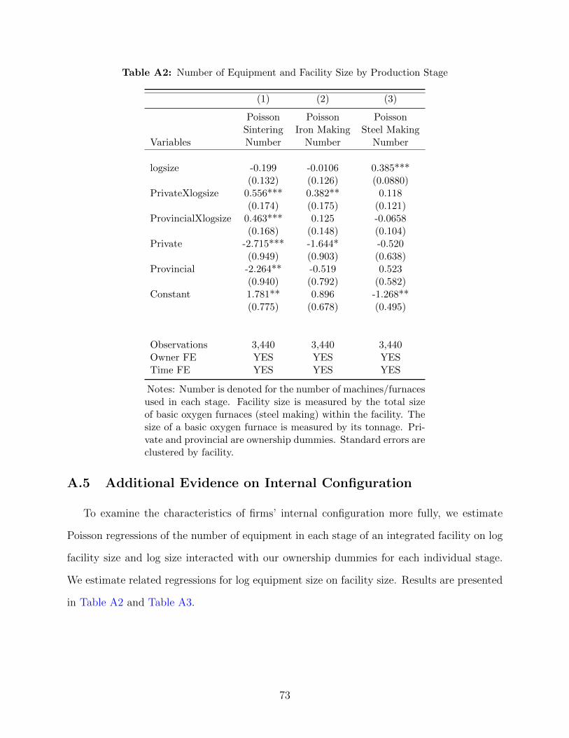
Table A2: Number of Equipment and Facility Size by Production Stage
(1) (2) (3)
Poisson Poisson PoissonSintering Iron Making Steel Making
Variables Number Number Number
logsize -0.199 -0.0106 0.385***(0.132) (0.126) (0.0880)
PrivateXlogsize 0.556*** 0.382** 0.118(0.174) (0.175) (0.121)
ProvincialXlogsize 0.463*** 0.125 -0.0658(0.168) (0.148) (0.104)
Private -2.715*** -1.644* -0.520(0.949) (0.903) (0.638)
Provincial -2.264** -0.519 0.523(0.940) (0.792) (0.582)
Constant 1.781** 0.896 -1.268**(0.775) (0.678) (0.495)
Observations 3,440 3,440 3,440Owner FE YES YES YESTime FE YES YES YES
Notes: Number is denoted for the number of machines/furnacesused in each stage. Facility size is measured by the total sizeof basic oxygen furnaces (steel making) within the facility. Thesize of a basic oxygen furnace is measured by its tonnage. Pri-vate and provincial are ownership dummies. Standard errors areclustered by facility.
A.5 Additional Evidence on Internal Configuration
To examine the characteristics of firms’ internal configuration more fully, we estimate
Poisson regressions of the number of equipment in each stage of an integrated facility on log
facility size and log size interacted with our ownership dummies for each individual stage.
We estimate related regressions for log equipment size on facility size. Results are presented
in Table A2 and Table A3.
73

Table A3: Average Equipment Size and Facility Size by Production Stage
(1) (2) (3)
Sintering Iron Making Steel MakingVariables logsize logsize logsize
logsize 0.718*** 0.765*** 0.609***(0.103) (0.122) (0.0788)
PrivateXlogsize -0.136 -0.287 -0.162(0.146) (0.184) (0.105)
ProvincialXlogsize -0.343** -0.102 0.00835(0.138) (0.139) (0.0938)
Private 0.507 1.072 0.747(0.754) (0.928) (0.543)
Provincial 1.624** 0.453 -0.192(0.753) (0.782) (0.531)
Constant 1.342** 3.032*** 1.349***(0.573) (0.702) (0.448)
Observations 3,440 3,440 3,440R-squared 0.344 0.536 0.593Owner FE YES YES YESTime FE YES YES YES
Notes: Facility size is measured by the total size of basic oxy-gen furnaces (steel making) within the facility. The size of asintering machine is measured by its e↵ective areas in m2; thesize of a blast furnace is measured by its e↵ective volume in m3;the size of a basic oxygen furnace is measured by its tonnage.Private and provincial are ownership dummies. Standard errorsare clustered by facility.
74

Table A4: Production Functions
(1) (2) (3) (4) (5) (6)sintering iron making steel making
VARIABLES ols gmm ols gmm ols gmm
l 0.215*** 0.187*** 0.303*** 0.253*** 0.341*** 0.353***(0.00843) (0.0151) (0.00706) (0.00266) (0.00787) (0.00301)
k 0.811*** 0.871*** 0.758*** 0.758*** 0.562*** 0.662***(0.00645) (0.00100) (0.00478) (0.000997)) (0.00514) (0.00151)
age -0.00115*** -0.000475 -0.000648*** 0.000187 -0.000584*** -0.00201*(0.000300) (0.00168) (0.000217) (0.000673) (0.000198) (0.00121)
Observations 6,389 6,389 9,353 9,353 8,514 8,514R-squared 0.829 0.825Ownership FE YES YES YES YES YES YESProvince FE YES YES YES YES YES YESTime FE YES YES YES YES YES YES
Note: Standard errors of production function coe�cients using GMM estimation are computed viabootstrap of 1,000 replications clustered by facility.
A.6 Leontief Production Function
We present the results based on Leontief production functions in Table A4 and Table A5.
75

Table A5: Productivity Di↵erences by Ownership and Size
(1) (2) (3) (4) (5) (6) (7) (8) (9)
Sintering Sintering Sintering Iron Iron Iron Steel Steel SteelVariables logtfp logtfp logtfp logtfp logtfp logtfp logtfp logtfp logtfp
logsize -0.0825*** -0.110*** -0.00663 -0.0115 -0.0902*** 0.0202(0.0232) (0.0340) (0.0141) (0.0379) (0.0236) (0.0728)
PrivateXlogsize -0.0224 -0.0873 -0.242**(0.0664) (0.0578) (0.109)
ProvincialXlogsize 0.0516 0.0240 -0.114(0.0466) (0.0406) (0.0774)
Private -0.111** -0.142*** -0.0495 0.0670** 0.0634* 0.616 0.147*** 0.0968* 1.160**(0.0513) (0.0484) (0.319) (0.0339) (0.0370) (0.391) (0.0538) (0.0567) (0.480)
Provincial -0.0973** -0.115*** -0.365 0.0213 0.0200 -0.142 0.0694* 0.0336 0.567(0.0444) (0.0410) (0.235) (0.0321) (0.0328) (0.296) (0.0401) (0.0412) (0.375)
Constant 0.0367 0.434*** 0.572*** -0.120*** -0.0751 -0.0418 -0.159*** 0.259** -0.261(0.0368) (0.113) (0.166) (0.0370) (0.110) (0.277) (0.0422) (0.121) (0.358)
Observations 8,728 8,728 8,728 11,852 11,852 11,852 8,538 8,538 8,538R-squared 0.016 0.039 0.043 0.017 0.018 0.024 0.034 0.064 0.078Time FE YES YES YES YES YES YES YES YES YES
Notes: Central state-owned facilities and their machines/furnaces are the omitted group. Private and provin-cial indicate ownership dummies. The size of a sintering machine is measured by its e↵ective areas in m2;the size of a blast furnace is measured by its e↵ective volume in m3; the size of a basic oxygen furnace ismeasured by its tonnage. Facility size is measured by the total size of basic oxygen furnaces (steel making)within the facility. Standard errors are clustered by machines/furnaces for stage-level analysis and by facilityfor facility-level analysis, but not corrected for the sampling error in constructed productivity.
76