Overview of Volume Rendering(Chapter for The Visualization Handbook, eds. C. Johnson and C. Hansen, Academic Press, 2005)

Arie Kaufman and Klaus MuellerCenter for Visual Computing Computer Science Department Stony Brook University

(version before final edits by the publisher)

INTRODUCTIONVolume visualization is a method of extracting meaningful

information from volumetric data using interactive graphics andimaging. It is concerned with volume data representation, model-ing, manipulation, and rendering [31][100][101][176]. Volumedata are 3D (possibly time-varying) entities that may have infor-mation inside them, might not consist of tangible surfaces andedges, or might be too voluminous to be represented geometrically.They are obtained by sampling, simulation, or modeling tech-niques. For example, a sequence of 2D slices obtained from Mag-netic Resonance Imaging (MRI), Computed Tomography (CT),functional MRI (fMRI), or Positron Emission Tomography (PET),is 3D reconstructed into a volume model and visualized for diag-nostic purposes or for planning of treatment or surgery. The sametechnology is often used with industrial CT for non-destructiveinspection of composite materials or mechanical parts. Similarly,confocal microscopes produce data which is visualized to study themorphology of biological structures. In many computational fields,such as in computational fluid dynamics, the results of simulationstypically running on a supercomputer are often visualized as vol-ume data for analysis and verification. Recently, the area of volumegraphics [104] has been expanding, and many traditional geomet-ric computer graphics applications, such as CAD and flight simula-tion, have been exploiting the advantages of volume techniques.

Over the years many techniques have been developed to ren-der volumetric data. Since methods for displaying geometric prim-itives were already well-established, most of the early methodsinvolve approximating a surface contained within the data usinggeometric primitives. When volumetric data are visualized using asurface rendering technique, a dimension of information is essen-tially lost. In response to this, volume rendering techniques weredeveloped that attempt to capture the entire 3D data in a single 2Dimage. Volume rendering convey more information than surfacerendering images, but at the cost of increased algorithm complex-ity, and consequently increased rendering times. To improve inter-activity in volume rendering, many optimization methods both forsoftware and for graphics accelerator implementations, as well asseveral special-purpose volume rendering machines, have beendeveloped.

VOLUMETRIC DATAA volumetric data set is typically a set V of samples (x,y,z,v),

also called voxels, representing the value v of some property of thedata, at a 3D location (x,y,z). If the value is simply a 0 or an integeri within a set I, with a value of 0 indicating background and thevalue of i indicating the presence of an object Oi, then the data isreferred to as binary data. The data may instead be multi-valued,with the value representing some measurable property of the data,including, for example, color, density, heat or pressure. The value vmay even be a vector, representing, for example, velocity at eachlocation, results from multiple scanning modalities, such as ana-tomical (CT, MRI) and functional imaging (PERT, fMRI), or color(RGB) triples, such as the Visible Human cryosection dataset [91].Finally, the volume data may be time-varying, in which case Vbecomes a 4D set of samples (x,y,z,t,v).

In general, the samples may be taken at purely random loca-tions in space, but in most cases the set V is isotropic containing

samples taken at regularly spaced intervals along three orthogonalaxes. When the spacing between samples along each axis is a con-stant, but there may be three different spacing constants for thethree axes the set V is anisotropic. Since the set of samples isdefined on a regular grid, a 3D array (also called the volume buffer,3D raster, or simply the volume) is typically used to store the val-ues, with the element location indicating position of the sample onthe grid. For this reason, the set V will be referred to as the array ofvalues V(x, y, z), which is defined only at grid locations. Alterna-tively, either rectilinear, curvilinear (structured), or unstructuredgrids, are employed (e.g., [240]). In a rectilinear grid the cells areaxis-aligned, but grid spacings along the axes are arbitrary. Whensuch a grid has been non-linearly transformed while preserving thegrid topology, the grid becomes curvilinear. Usually, the rectilineargrid defining the logical organization is called computationalspace, and the curvilinear grid is called physical space. Otherwisethe grid is called unstructured or irregular. An unstructured orirregular volume data is a collection of cells whose connectivityhas to be specified explicitly. These cells can be of an arbitraryshape such as tetrahedra, hexahedra, or prisms.

RENDERING VIA GEOMETRIC PRIMITIVESTo reduce the complexity of the volume rendering task, sev-

eral techniques have been developed which approximate a surfacecontained within the volumetric data by ways of geometric primi-tives, most commonly triangles, which can then be rendered usingconventional graphics accelerator hardware. A surface can bedefined by applying a binary segmentation function B(v) to the vol-umetric data, where B(v) evaluates to 1 if the value v is consideredpart of the object, and evaluates to 0 if the value v is part of thebackground. The surface is then contained in the region where B(v)changes from 0 to 1.

Most commonly, B(v) is either a step function (where viso is called the iso-value), or an

interval [v1,v2] in which (where [v1,v2] iscalled the iso-interval). For the former, the resulting surface iscalled the iso-surface, while for the latter the resulting structure iscalled the iso-contour. Several methods for extracting and render-ing iso-surfaces have been developed, a few are briefly describedhere. The Marching Cubes algorithm [136] was developed toapproximate an iso-valued surface with a triangle mesh. The algo-rithm breaks down the ways in which a surface can pass through agrid cell into 256 cases, based on the B(v) membership of the 8voxels that form the cell’s vertices. By ways of symmetry, the 256cases reduce to 15 base topologies, although some of these haveduals, and a technique called Asymptotic Decider [185] can beapplied to select the correct dual case and thus prevent the inci-dence of holes in the triangle mesh. For each of the 15 cases (andtheir duals), a generic set of triangles representing the surface isstored in a look-up table. Each cell through which a surface passesmaps to one of the base cases, with the actual triangle vertex loca-tions being determined using linear interpolation of the cell verti-ces on the cell edges (see Fig. 1). A normal value is estimated foreach triangle vertex, and standard graphics hardware can be uti-lized to project the triangles, resulting in a relatively smoothshaded image of the iso-valued surface.

When rendering a sufficiently large data set with the March-

B v( ) 1 v viso≥∀,=B v( ) 1 v v1 v2,[ ]∈∀,=

1

ing Cubes algorithm, with an average of 3 triangles per cell, mil-lions of triangles may be generated, and this can impede interactiverendering of the generated polygon mesh. To reduce the number oftriangles, one may either post-process the mesh by applying one ofthe many mesh decimation methods (see e.g., [63][88][220]), orproduce a reduced set of primitives in the mesh generation process,via a feature-sensitive octree method [223] or discretized MarchingCubes [170]. The fact that during viewing many of the primitivesmay map to a single pixel on the image plane led to the develop-ment of screen-adaptive surface rendering algorithms that use 3Dpoints as the geometric primitive. One such algorithm is DividingCubes [36], which subdivides each cell through which a surfacepasses into subcells. The number of divisions is selected such thatthe subcells project onto a single pixel on the image plane. Anotheralgorithm which uses 3D points as the geometric primitive is theTrimmed Voxel Lists method [235]. Instead of subdividing, thismethod uses one 3D point (with normal) per visible surface cell,projecting that cell on up to three pixels of the image plane toinsure coverage in the image.

The traditional Marching Cubes algorithms simply marchesacross the grid and inspects every cell for a possible iso-surface.This can be wasteful when users want to interactively change theiso-value viso and -surface to explore the different surfaces embed-ded in the data. By realizing that an iso-surface can only passthrough a cell if at least one voxel has a value above or equal visoand at least one voxel has a value below or equal viso, one candevise data structures that only inspect cells where this criterion isfulfilled. Examples are the NOISE algorithm [135] that uses a K-Dtree embedded into span-space for quickly identifying the candi-date cells (this method was later improved by [35] who used aninterval tree), as well as the ISSUE algorithm [224]. Finally, sinceoften triangles are generated that are later occluded during the ren-dering process, it is advisable to visit the cells in front-to-backorder and only extract and render triangles that fall outside previ-ously occluded areas [62].

DIRECT VOLUME RENDERING: PRELUDERepresenting a surface contained within a volumetric data set

using geometric primitives can be useful in many applications,however, there are several main drawbacks to this approach. First,geometric primitives can only approximate surfaces containedwithin the original data. Adequate approximations may require anexcessive amount of geometric primitives. Therefore, a trade-offmust be made between accuracy and space requirements. Second,since only a surface representation is used, much of the informa-tion contained within the data is lost during the rendering process.For example, in CT scanned data useful information is containednot only on the surfaces, but within the data as well. Also, amor-

phous phenomena, such as clouds, fog, and fire cannot be ade-quately represented using surfaces, and therefore must have avolumetric representation, and must be displayed using volumerendering techniques.

However, before moving to techniques that visualize the datadirectly, without going through an intermediate surface extractionstep, we first discuss in the next section some of the general princi-ples that govern the theory of discretized functions and signals,such as the discrete volume data. We also present some specializedtheoretical concepts, more relevant in the context of volume visual-ization.

VOLUMETRIC FUNCTION INTERPOLATION The volume grid V only defines the value of some measured

property f(x,y,z) at discrete locations in space. If one requires thevalue of f(x,y,z) at an off-grid location (x,y,z), a process calledinterpolation must be employed to estimate the unknown valuefrom the known grid samples V(x,y,z). There are many possibleinterpolation functions (also called filters or filter kernels). Thesimplest interpolation function is known as zero-order interpola-tion, which is actually just a nearest-neighbor function. i.e., thevalue at any location (x,y,z) is simply that of the grid sample closestto that location:

(1)

which gives rise to a box filter (black curve in Fig. 4). With thisinterpolation method there is a region of constant value aroundeach sample in V. The human eye is very sensitive to the jaggededges and unpleasant staircasing that result from a zero-order inter-polation, and therefore this kind of interpolation gives generallythe poorest visual results (see Fig. 3a).

Linear or first-order interpolation (magenta curve in Fig. 4) isthe next-best choice, and its 2D and 3D versions are called bi-lin-ear and tri-linear interpolation, respectively. It can be written as 3stages of 7 linear interpolations, since the filter function is separa-ble in higher dimensions. The first 4 linear interpolations are alongx:

(2)

Using these results, 2 linear interpolations along y follow:

(3)

One final interpolation along z yields the interpolation result:

200 100

110

50 80

7090

Figure 1: A grid cell with voxel values as indicated, intersectedby an iso-surface (iso-value=125). This is base case #1 of theMarching Cubes algorithm: a single triangle separating surfaceinterior (black vertex) from exterior (white vertices). The posi-tions of the triangle vertices are estimated by linear interpolationalong the cell edges.

vmin

vmax

viso

viso

candidate cells

Figure 2: Each grid cell is characterized by its lowest (vmin) andits highest (vmax) voxel value, and represented by a point in spanspace. Given an iso-value viso, only cells that satisfy both

and contain the iso-surface and arequickly extracted from a K-D tree [135] or interval-tree [35]embedding of the span-space points.

vmin viso≤ vmax viso≥

f x y z ), ,( ) V round x( ) round y( ) round z( ),,( )=

f u v0 1, w0 1,, ,( )

1 u–( ) V 0 v0 1, w0 1,, ,( ) uV 1 v0 1, w0 1,, ,( )+( )=

f u v w0 1,, ,( ) 1 v–( )f u 0 w0 1,, ,( ) vf u 1 w0 1,, ,( )+=

2

(4)

Here the u,v,w are the distances (assuming a cell of size 13, withoutloss of generality) of the sample at (x,y,z) from the lower, left, rearvoxel in the cell containing the sample point (e.g., the voxel withvalue 50 in Fig. 1). A function interpolated with a linear filter nolonger suffers from staircase artifacts (see Fig. 3b). However, it hasdiscontinuous derivatives at cell boundaries, which can lead tonoticeable banding when the visual quantities change rapidly fromone cell to the next.

A second-order interpolation filter that yields a f(x,y,z) with acontinuous first derivative is the cardinal spline function, whose1D function is given by (see blue curve in Fig. 4):

(5)

Here, u measures the distance of the sample location to the gridpoints that fall within the extent of the kernel, and a=-0.5 yields theCatmull-Rom spline which interpolates a discrete function with thelowest third-order error [107]. The 3D version of this filter h(u,v,w)is separable, i.e., h(u,v,w)=h(u)h(v)h(w), and therefore interpola-tion in 3D can be written as a 3-stage nested loop.

A more general form of the cubic function has two parametersand the interpolation results obtained with different settings ofthese parameters has been investigated by Mitchell and Netravali[165]. In fact, the choice of filters and their parameters always pre-sents trade-offs between the sensitivity to noise, sampling fre-quency ripple, aliasing (see below), ringing, and blurring, and thereis no optimal setting that works for all applications. Marschner andLobb [151] extended the filter discussion to volume rendering andcreated a challenging volumetric test function with a uniform fre-quency spectrum that can be employed to visually observe thecharacteristics of different filters (see Fig. 5). Finally, Möller et al.[167] applied a Taylor series expansion to devise a set of optimaln-th order filters that minimize the (n+1)-th order error.

Generally, higher filter quality comes at the price of widerspatial extent (compare Fig. 4) and therefore larger computationaleffort. The best filter possible in the numerical sense is the sinc fil-ter, but it has infinite spatial extent and also tends to noticeableringing [165]. Sinc filters make excellent, albeit expensive, inter-polation filters when used in truncated form and multiplied by awindow function [151][252], possibly adaptive to local detail[148]. In practice, first-order or linear filters give satisfactoryresults for most applications, providing good cost-quality trade-offs, but cubic filters are also used. Zero-order filters give accept-able results when the discrete function has already been sampled ata very high rate, for example in high-definition function lookuptables [270].

All filters presented thus far are grid-interpolating filters, i.e.,

their interpolation yields f(x,y,z) = V(x,y,z) at grid points [254].When presented with a uniform grid signal they also interpolate auniform f(x,y,z) everywhere. This is not the case with a Gaussianfilter function (red curve in Fig. 4) which can be written as:

(6)

Here, a determines the width of the filter and b is a scale factor.The Gaussian has infinite continuity in the interpolated function’sderivative, but it introduces a slight ripple (about 0.1%) into aninterpolated uniform function. The Gaussian is most popular whena radially symmetric interpolation kernel is needed [268][183] andfor grids that assume that the frequency spectrum of f(x,y,z) is radi-ally bandlimited [253][182].

It should be noted that interpolation cannot restore sharpedges that may have existed in the original function forg(x,y,z) priorto sampling into the grid. Filtering will always smooth or lowpassthe original function somewhat. Non-linear filter kernels [93] ortransformations of the interpolated results [180] are needed to rec-reate sharp edges, as we shall see later.

A frequent artifact that can occur is aliasing. It results frominadequate sampling and gives rise to strange patterns that did notexist in the sampled signal. Proper pre-filtering (bandlimiting) hasto be performed whenever a signal is sampled below its Nyquistlimit, i.e., twice the maximum frequency that occurs in the signal.Filtering after aliasing will not undo these adverse effects. Fig. 6illustrates this by ways of an example, and the interested readermay consult standard texts, such as [281] and [57], for more detail.

The gradient of f(x,y,z) is also of great interest in volume visu-alization, mostly for the purpose of estimating the amount of lightreflected from volumetric surfaces towards the eye (for example,strong gradients indicate stronger surfaces and therefore strongerreflections). There are three popular methods to estimate a gradientfrom the volume data [166]. The first computes the gradient vectorat each grid point via a process called central differencing:

Figure 3: Magnification via interpolation with (a) a box filter;and (b) a bi-linear filter. The latter gives a much more pleasingresult.

(a) (b)

f x y z, ,( ) f u v w, ,( ) 1 w–( )f u v 0, ,( ) wf u v 1, ,( )+= =

h u( )a 2+( ) u 3 a 3+( ) u 2– 1+ 0 u 1<≤

a u 3 5a u 2– 8a u 4a–+ 1 u 2≤ ≤0 u 2>⎝

⎜⎜⎜⎛

=

Figure 4: Popular filters in the spatial domain: box (black), lin-ear (magenta), cubic (blue), Gaussian (red)

Figure 5: Marschner-Lobb test function, sampled into a 203

grid: (a) the whole function, (b) close-up, reconstructed and ren-dered with a cubic filter.

h u v w, ,( ) b e a u2 v2 w2+ +( )–⋅=

3

(7)

and then interpolates the gradient vectors at a (x,y,z) using any ofthe filters described above. The second method also uses centraldifferencing, but it does it at (x,y,z) by interpolating the requiredsupport samples on the fly. The third method is the most direct andemploys a gradient filter [11] in each of the three axis directions toestimate the gradients. These three gradient filters could be simplythe (u,v,w) partial derivatives of the filters described above or theycould be a set of optimized filters [166]. The third method gives thebest results since it only performs one interpolation step, while theother two methods have lower complexity and often have practicalapplication-specific advantages. An important observation is thatgradients are much more sensitive to the quality of the interpola-tion filter since they are used in illumination calculations, whichconsist of higher-order functions that involve the normal vectors,which in turn are calculated from the gradients via normalization[167].

VOLUME RENDERING TECHNIQUESIn the next subsections various fundamental volume rendering

techniques are explored. Volume rendering or direct volume ren-dering is the process of creating a 2D image directly from 3D volu-metric data, hence it is often called direct volume rendering.Although several of the methods described in these subsectionsrender surfaces contained within volumetric data, these methodsoperate on the actual data samples, without generating the interme-diate geometric primitive representations used by the algorithms inthe previous section.

Volume rendering can be achieved using an object-order, animage-order, or a domain-based technique. Hybrid techniqueshave also been proposed. Object-order volume rendering tech-

niques use a forward mapping scheme where the volume data ismapped onto the image plane. In image-order algorithms, a back-ward mapping scheme is used where rays are cast from each pixelin the image plane through the volume data to determine the finalpixel value. In a domain-based technique the spatial volume data isfirst transformed into an alternative domain, such as compression,frequency, and wavelet, and then a projection is generated directlyfrom that domain.

Image-Order TechniquesThere are four basic volume rendering modes: X-ray render-

ing, Maximum Intensity Projection (MIP), iso-surface renderingand full volume rendering, where the third mode is just a specialcase of the fourth. These four modes share two common opera-tions: (i) They all cast rays from the image pixels, sampling thegrid at discrete locations along their paths, and (ii) they all obtainthe samples via interpolation, using the methods described in theprevious section. The modes differ, however, in how the samplestaken along a ray are combined. In X-ray, the interpolated samplesare simply summed, giving rise to a typical image obtained in pro-jective diagnostic imaging (Fig. 7a), while in MIP only the interpo-lated sample with the largest value is written to the pixel (Fig. 7b).In full volume rendering (Fig. 7c and d), on the other hand, theinterpolated samples are further processed to simulate the lighttransport within a volumetric medium according to one of manypossible models. In the remainder of this section, we shall concen-trate on the full volume rendering mode since it provides the great-est degree of freedom, although rendering algorithms have beenproposed that merge the different modes into a hybrid image gener-ation model [80].

The fundamental element in full volume rendering is the vol-ume rendering integral. In this section we shall assume the low-albedo scenario, in which a certain light ray only scatters oncebefore leaving the volume. The low-albedo optical model was firstdescribed by [14] and [98], and then formally derived by [152]. Itcomputes, for each cast ray, the quantity Iλ(x,r), which is theamount of light of wavelength λ coming from ray direction r that isreceived at point x on the image plane:

(8)

Here L is the length of ray r. We can think of the volume as beingcomposed of particles with certain mass density values µ (Max

(a)

(b) (c)

(d)

(e)

Figure 6: Anti-aliasing: (a) original image; (b) reduction by sim-ple subsampling - disturbing patterns emerge, caused by aliasingthe higher frequency content; (c) blurring of (b) does not elimi-nate patterns; (d) pre-filtering (blurring) of the original imagereduces its high frequency content; (e) subsampling of (d) doesnot cause aliasing due to the prior bandlimiting operation.

gx

gy

gz

V x 1 y z, ,–( )V x y 1– z, ,( )V x y z 1–, ,( )

V x 1 y z, ,+( )V x y 1+ z, ,( )V x y z 1+, ,( )

–=

Figure 7: CT head rendered in the four main volume renderingmodes: (a) X-ray; (b) MIP; (c) Iso-surface; (d) Translucent.

(a)

(c)

(b)

(d)

Iλ x r,( ) Cλ s( )µ s( ) µ t( ) td0

s∫–

⎝ ⎠⎜ ⎟⎛ ⎞

exp sd0

L∫=

4

calls them light extinction values [152]). These values, as well asthe other quantities in this integral, are derived from the interpo-lated volume densities f(x,y,z) via some mapping function. The par-ticles can contribute light to the ray in three different ways: viaemission [215], transmission, and reflection [258], thusCλ(s)=Eλ(s)+Tλ(s)+Rλ(s). The latter two terms, Tλ and Rλ, trans-form light received from surrounding light sources, while theformer, Eλ, is due to the light-generating capacity of the particle.The reflection term takes into account the specular and diffusematerial properties of the particles. To account for the higherreflectivity of particles with larger mass densities, one must weightCλ by µ. In low-albedo, we only track the light that is received onthe image plane. Thus, in (8), Cλ is the portion of the light of wave-length λ available at location s that is transported in the direction ofr. This light then gets attenuated by the mass densities of the parti-cles along r, according to the exponential attenuation function.

Rλ(s) is computed via the standard illumination equation [57]:

(9)

where we have dropped the subscript λ for reasons of brevity.Here, Ca is the ambient color, ka is the ambient material coeffi-cient, Cl is the color of the light source, Co is the color of the object(determined by the density-color mapping function), kd is the dif-fuse material coefficient, N is the normal vector (determined by thegradient), L is the light direction vector, ks is the specular materialcoefficient, H is the halfvector, and ns is the Phong exponent.

Equation (8) only models the attenuation of light from s to theeye (blue ray in Fig. 8). But the light received at s is also attenuatedby the volume densities on its path from the light source to s (redray in Fig. 8). This gives rise to the following term for Cl in (9),which is now dependent on the location s:

(10)

Here, CL is the color of the lightsource and T is the distance from sto the light source (see Fig. 8). The inclusion of this term into (9)produces volumetric shadows, which give greater realism to theimage [191][290] (see Fig. 9). In practice, applications that com-pute volumetric shadows are less common, due to the added com-putational complexity, but an interactive hardware-based approachhas been recently proposed [113][114].

The analytic volume rendering integral cannot, in the generalcase, be computed efficiently, if at all, and therefore a variety ofapproximations are in use. An approximation of (8) can be formu-lated using a discrete Riemann sum, where the rays interpolate aset of samples, most commonly spaced apart by a distance ∆s:

(11)

A few more approximations make the computation of thisequation more efficient. First, the transparency t(i∆s) is defined as

. Transparency assumes values in the range [0.0,1.0]. The opacity is the inverse of thetransparency. Further, the exponential term in (11) can be approxi-mated by the first two terms of its Taylor series expansion:

. Then, one can write:. This transforms (11) into the

well-known compositing equation:

(12)

This is a recursive equation in (1-α) and gives rise to the recursivefront-to-back compositing formula [127][207]:

(13)

Thus, a practical implementation of volumetric ray would traversethe volume from front to back, calculating colors and opacities ateach sampling site, weighting these colors and opacities by the cur-rent accumulated transparency (1-α), and adding these terms to theaccumulated color and transparency to form the terms for the nextsample along the ray. An attractive property of the front-to-backtraversal is that a ray can be stopped once α approaches 1.0, whichmeans that light originating from structures further back is com-pletely blocked by the cumulative opaque material in front. Thisprovides for accelerated rendering and is called early ray termina-tion. An alternative form of (13) is the back-to-front compositingequation:

(14)

Back-to-front compositing is a generalization of the Painter’s algo-rithm and does not enjoy speed-up opportunities of early ray termi-nation and is therefore less frequently used.

Equation (12) assumes that a ray interpolates a volume thatstores at each grid point a color vector (usually a (red, green, blue)= RGB triple) as well as an α value [127][128]. There, the colorsare obtained by shading each grid point using (9). Before wedescribe the alternative representation, let us first discuss how thevoxel densities are mapped to the colors Co in (9).

The mapping is implemented as a set of mapping functions,often implemented as 2D tables, called transfer functions. By waysof the transfer functions, users can interactively change the proper-ties of the volume dataset. Most applications give access to fourmapping functions: R(d), G(d), B(d), A(d), where d is the value of agrid voxel, typically in the range of [0,255] for 8-bit volume data.Thus, users can specify semi-transparent materials by mappingtheir densities to opacities < 1.0, which allows rays to acquire amix of colors that is due to all traversed materials. More advanced

R s( ) kaCa kdClCo s( ) N s( ) L s( )⋅( ) ksCl N s( ) H s( )⋅( )ns+ +=

Figure 8: Transport of light to the eye.

sample point s

delivered lightlight source

reflected light

eye

Cl s( ) CL µ t( ) tds

T

∫–⎝ ⎠⎛ ⎞exp=

Iλ x r,( ) Cλ i∆s( )µ i∆s( )∆s µ j∆s( )∆s–( )exp

j 0=

i 1–

∏i 0=

L ∆s⁄ 1–

∑=Figure 9: CT lobster rendered without shadows (left) and withshadows (right). The shadows on the wall behind the lobster aswell as the self-shadowing of the legs creates greater realism.

µ i∆s( )∆s–( )expα i∆s( ) 1 t i∆s( )–( )=

t i∆s( ) µ i∆s( )∆s–( )exp= 1 µ i∆s( )∆s–≈µ i∆s( )∆s 1 t i∆s( )–≈ α i∆s( )=

Iλ x r,( ) Cλ i∆s( )α i∆s( ) 1 α j∆s( )–( )

j 0=

i 1–

∏⋅

i 0=

L ∆s⁄ 1–

∑=

c C i∆s( )α i∆s( ) 1 α–( ) c+=α α i∆s( ) 1 α–( ) α+=

c c 1 α i∆s( )–( ) C i∆s( )+=α α 1 α i∆s( )–( ) α i∆s( )+=

5

applications give users also access to transfer functions that mapks(d), kd(d), ns(d), and others. Wittenbrink pointed out that the col-ors and opacities at each voxel should be multiplied prior to inter-polation to avoid artifacts on object boundaries [280].

The model in (12) is called the pre-classified model, sincevoxel densities are mapped to colors and opacities prior to interpo-lation. This model cannot resolve high frequency detail in thetransfer functions (see Fig. 10 for an example), and also typicallygives blurry images under magnification [180]. An alternativemodel that is more often used is the post-classified model. Here,the raw volume values are interpolated by the rays, and the interpo-lation result is mapped to color and opacity:

(15)

The function value f(i∆s) and the gradient vector g(i∆s) are inter-polated from fd(x,y,z) using a 3D interpolation kernel, and Cλ and αare now the transfer and shading functions that translate the inter-polated volume function values into color and opacity. This gener-ates considerably sharper images (see Fig. 11).

A quick transition from 0 to 1 at some density value di in theopacity transfer function selects the iso-surface diso=di. Thus, iso-surface rendering is merely a subset of full volume rendering,where the ray hits a material with d=diso and then immediatelybecomes opaque and terminates.

Post-classified rendering only eliminates some of the prob-lems that come with busy transfer functions. Consider againFig. 10a, and now assume a very narrow peak in the transfer func-tion at d12. With this kind of transfer function, a ray point-samplingthe volume at s may easily miss to interpolate d12, but may haveinterpolated it, had it just sampled the volume at s+δs. Pre-inte-grated transfer functions [55] solve this problem by pre-computinga 2D table that stores the analytical volume rendering integrationfor all possible density pairs (df,db). This table is then indexed dur-ing rendering by each ray sample pair (db, df), interpolated at sam-ple locations ∆s apart (see Fig. 10b). The pre-integration assumes apiecewise linear function within the density pairs, and thus guaran-tees that no transfer function detail falling between two interpo-lated (df, db) fails to be considered in the discrete ray integration.

Object-Order Techniques

Object-order techniques decompose the volume into a set ofbasis elements or basis functions which are individually projectedto the screen and assemble into an image. If the volume renderingmode is X-ray or MIP, then the basis functions can be projected inany order, since in X-ray and MIP the volume rendering integraldegenerates to a commutative sum or MAX operation. In contrast,depth ordering is required when solving for the generalized volumerendering integral (8). Early work represented the voxels as dis-joint cubes, which gave rise to the cuberille representation[68][83]. Since a cube is equivalent to a nearest neighbor kernel,the rendering results were inferior. Therefore, more recentapproaches have turned to kernels of higher quality.

To better understand the issues associated with object-orderprojection it helps to view the volume as a field of basis functionsh, with one such basis kernel located at each grid point where it ismodulated by the grid point’s value (see Fig. 12 where two suchkernels are shown). This ensemble of modulated basis functionsthen makes up the continuous object representation, i.e., one couldinterpolate a sample anywhere in the volume by simply adding upthe contributions of the modulated kernels that overlap at the loca-tion of the sample value. Hence, one could still traverse thisensemble with rays and render it in image-order. However, a moreefficient method emerges when realizing that the contribution of avoxel j with value dj is given by , where s follows theline of kernel integration along the ray. Further, if the basis kernelis radially symmetric, then the integration is independentof the viewing direction. Therefore, one can perform a pre-integra-tion of and store the result into a lookup-table. This tableis called the kernel footprint, and the kernel projection process isreferred to as kernel splatting or simply, splatting. If the kernel is aGaussian, then the footprint is a Gaussian as well. Since the kernelis identical for all voxels, we can use it for all voxels. We can gen-erate an image by going through the list of object voxels in depth-order and performing the following steps for each (see againFig. 12): (i) Calculate the screen-space coordinate of the projectedgrid point; (ii) center the footprint around that point and stretch itaccording to the image magnification factor; (iii) rasterize the foot-print to the screen, using the pre-integrated footprint table and mul-tiplying the indexed values by the voxel’s value [268][269][270].This rasterization can either be performed via fast DDA procedures[147][174], or in graphics hardware, by texture-mapping the foot-print (basis image) onto a polygon [42].

There are three types of splatting: composite-only, axis-

density

color

d1 d2

Figure 10: Transfer function aliasing. When the volume is ren-dered pre-classified, then both the red (density d1) and the blue(density d2) voxels receive a color of zero, according to thetransfer function shown on the left. At ray sampling this voxelneighborhood at s would then interpolate a color of zero as well.On the other hand, in post-classified rendering, the ray at s wouldinterpolate a density close to d12 (between d1 and d2) andretrieve the strong color associated with d12 in the transfer func-tion.

sampling site sd12

dfdb

(a) (b)

Iλ x r,( ) =

Cλ f i∆s( ) g i∆s( ),( )α f i∆s( )( ) 1 α f j∆s( )( )–( )

j 0=

i 1–

∏i 0=

L ∆s⁄ 1–

∑

Figure 11: Pre-classified (left column) vs. post-classified ren-dering (right column). The latter yields sharper images since theopacity and color classification is performed after interpolation.This eliminates the blurry edges introduced by the interpolationfilter.

dj h s( ) sd∫⋅

h s( ) sd∫h s( ) sd∫

6

aligned sheet-buffered, and image-aligned sheet-buffered splatting.The composite-only method was proposed first [269] and is themost basic one (see Fig. 12). Here, the object points are traversedin either front-to-back or back-to-front order. Each is first assigneda color and opacity using the shading equation (9) and the transferfunctions. Then, each point is splatted into the screen’s color andopacity buffers and the result is composited with the present image(Equation (13)). In this approach, color bleeding and slight spar-kling artifacts in animated viewing may be noticeable since theinterpolation and compositing operations cannot be separated dueto the pre-integration of the basis (interpolation) kernel [270].

An attempt to solve this problem gave way to the axis-alignedsheet-buffered splatting approach [268] (see Fig. 13a). Here, thegrid points are organized into sheets (basically the volume slicesmost parallel to the image plane), assigned a color and opacity, andsplatted into the sheet’s color and opacity buffers. The importantdifference is that now all splats within a sheet are added and notcomposited, while only subsequent sheets are composited. Thisprevents potential color bleeding of voxels located in consecutivesheets, due to the more accurate reconstruction of the opacity layer.The fact that the voxel sheets must be formed by the volume slicesmost parallel to the viewing axis leads to a sudden switch of thecompositing order when the major viewing direction changes andan orthogonal stack of volume slices must be used to organize thevoxels. This causes noticeable popping artifacts where some sur-faces suddenly reflect less light and others more [173]. The solu-tion to this problem is to align the compositing sheet with theimage plane at all times, which gives rise to the image-alignedsheet-buffered splatting approach [173] (see Fig. 13b). Here, a slabis advanced across the volume and all kernels that intersect the slabare sliced and projected. Kernel slices can be pre-integrated intofootprints as well, and thus this sheet-buffered approach differsfrom the original one in that each voxel has to be considered morethan once. The image-aligned splatting method provides the mostaccurate reconstruction of the voxel field prior to compositing andeliminates both color bleeding and popping artifacts. It is also bestsuited for post-classified rendering since the density (and gradient)field is reconstructed accurately in each sheet. However, it is moreexpensive due to the multiple splatting of a voxel.

The divergence of rays under perspective viewing causesundersampling of the volume portions further away from the view-point (see Fig. 14). This leads to aliasing in these areas. As wasdemonstrated in Fig. 6, lowpassing can eliminate the artifactscaused by aliasing and replace them by blur (see Fig. 15). For per-spective rendering the amount of required lowpassing increaseswith distance from the viewpoint. The kernel-based approachescan achieve this progressive lowpassing by simply stretching thefootprints of the voxels as a function of depth, since stretched ker-nels act as lowpass filters (see Fig. 14). EWA (Elliptical WeightedAverage) Splatting [293] provides a general framework to definethe screen-space shape of the footprints, and their mapping into ageneric footprint, for generalized grids under perspective viewing.An equivalent approach for raycasting is to split the rays in moredistant volume slices to always maintain the proper sampling rate[190]. Kreeger et al. [118] proposed an improvement of thisscheme that splits and merges rays in an optimal way.

A major advantage of object-order methods is that only thepoints (or other basis primitives, such as tetrahedral or hexagonalcells [273]) which make up the object must be stored. This can beadvantageous when the object has an intricate shape, with manypockets of empty space [159]. While raycasting would spend mucheffort traversing (and storing) the empty space, kernel-based orpoint-based objects will not consider the empty space, neither dur-ing rendering nor for storage. However, there are trade-offs, sincethe rasterization of a footprint takes more time than the commonlyused trilinear interpolation of ray samples, since the radially sym-metric kernels employed for splatting must be larger than the trilin-ear kernels to ensure proper blending. Hence, objects with compactstructure are more favorably rendered with image-order methodsor hybrid methods (see next section). Another disadvantage ofobject-order methods is that early ray termination is not availableto cull occluded material early from the rendering pipeline. The

compositesplat

screen

Figure 12: Object-order volume rendering with kernel splattingimplemented as footprint mapping.

add

composite

add

composite

Figure 13: Sheet-buffered splatting: (a) axis-aligned - the entirekernel within the current sheet is added, (b) image-aligned - onlyslices of the kernels intersected by the current sheet-slab areadded.

(a) (b)

Figure 14: Stretching the basis functions in volume layers z>zk,where the sampling rate of the ray grid is progressively less thanthe volume resolution.

zk

Figure 15: Anti-aliased splatting: (Left) A checkerboard tunnelrendered in perspective with equal sized splats. Aliasing occursat distances beyond the black square. (Right) The same checker-board tunnel rendered with scaled splats. The aliasing has beenreplaced by blur.

7

object-order equivalent is early point elimination, which is moredifficult to achieve than early ray termination. Finally, image-ordermethods allow the extension of raycasting to raytracing, where sec-ondary and higher-order rays are spawned at reflection sites. Thisfacilitates mirroring on shiny surfaces, inter-reflections betweenobjects, and soft shadows.

There are a number of ways to store and manage point-basedobjects. These schemes are mainly distinguished by their ability toexploit spatial coherence during rendering. The lack of spatialcoherence requires more depth sorting during rendering and alsomeans more storage for spatial parameters. The least spatial coher-ence results from storing the points sorted by density [41]. This hasthe advantage that irrelevant points, being assigned transparent val-ues in the transfer functions, can be quickly culled from the render-ing pipeline. However, it requires that (x,y,z) coordinates and,possibly gradient vectors, are stored along with the points sinceneighborhood relations are completely lost. It also requires that allpoints be view-transformed first before they can be culled due toocclusion or exclusion from the viewing pyramid. The method alsorequires that the points be depth-sorted during rendering, or atleast, tossed into depth bins [177]. A compromise is struck by Ihmand Lee [94] who sort points by density within volume slices only,which gives implicit depth-ordering when used in conjunction withan axis-aligned sheet-buffer method. A number of approaches existthat organize the points into RLE (Run Length Encoded) lists,which allow the spatial coordinates to be incrementally computedwhen traversing the runs [108][182]. However, these approachesdo not allow points to be easily culled based on their density value.Finally, one may also decompose the volume into a spatial octreeand maintain a list of voxels in each node. This provides depthsorting on the node-level.

A number of surface-based splatting methods have also beendescribed. These do not provide the flexibility of volume explora-tion via transfer functions, since the original volume is discardedafter the surface has been extracted. They only allow a fixed geo-metric representation of the object that can be viewed at differentorientations and with different shadings. A popular method isshell-rendering [259] which extracts from the volume (possiblywith a sophisticated segmentation algorithm) a certain thin or thicksurface or contour and represents it as a closed shell of points.Shell-rendering is fast since the number of points is minimized andits data structure used has high cache coherence. More advancedpoint-based surface rendering methods are QSplat [214], Surfels[201], and Surface Splats [292], which have been predominantlydeveloped for point-clouds obtained with range scanners, but canalso be used for surfaces extracted from volumes [293].

Hybrid TechniquesHybrid techniques seek to combine the advantages of the

image-order and object-order methods, i.e., they use object-cen-tered storage for fast selection of relevant material (which is a hall-mark of object-order methods) and they use early ray terminationfor fast occlusion culling (which is a hallmark of image-ordermethods).

The shear-warp algorithm [120] is such a hybrid method. Inshear-warp, the volume is rendered by a simultaneous traversal ofRLE-encoded voxel and pixel runs, where opaque pixels and trans-parent voxels are efficiently skipped during these traversals (seeFig. 16a). Further speed comes from the fact that sampling onlyoccurs in the volume slices via bilinear interpolation, and that theray grid resolution matches that of the volume slices, and thereforethe same bilinear weights can be used for all rays within a slice(see Fig. 16b). The caveat is that the image must first be renderedfrom a sheared volume onto a so-called base-plane, that is alignedwith the volume slice most parallel to the true image plane(Fig. 16a). After completing the base-plane rendering, the base

plane image must be warped onto the true image plane and theresulting image is displayed. All of this combined enables framer-ates in excess of 10 frames/s on current PC processors, for a 1283

volume. There are a number of compromises that had to be made inthe process:• Since the interpolation only occurs within one slice at a time,

more accurate tri-linear interpolation reduces to less accurate bi-linear interpolation and the ray sampling distance varies between1 and , depending on the view orientation. This leads to alias-ing and staircasing effects at viewing angles near 45°.

• Since the volume is run-length one needs to use three sets ofvoxel encodings (but it could be reduced to two [249]), one forthe each major viewing direction. This triples the memoryrequired for the runs, but in return, the RLE encoding saves con-siderable space.

• Since there is only one interpolated value per voxel-slice 4-neighborhood, zooming can only occur during the warping phaseand not during the projection phase. This leads to considerableblurring artifacts at zoom factors greater than 2. The post-render-ing magnification in fact is a major source of the speedup for theshear-warp algorithm.

An implementation of the shear-warp algorithm is publiclyavailable as the volpack package [90] from Stanford University.

Domain Volume RenderingIn domain rendering, the spatial 3D data is first transformed

into another domain, such as compression, frequency, and waveletdomain, and then a projection is generated directly from thatdomain or with the help of information from that domain. The fre-quency domain rendering applies the Fourier slice projection theo-rem, which states that a projection of the 3D data volume from acertain view direction can be obtained by extracting a 2D slice per-

Figure 16: The shear-warp algorithm. (a) mechanism, (b) inter-polation scheme.

(a)

(b)

workskip

non-transparent RLE run

baseplane

post-rendering warp

work skip

skip

opaque run

image plane

ray sample points within slice

3

8

pendicular to that view direction out of the 3D Fourier spectrumand then inverse Fourier transforming it. This approach obtains the3D volume projection directly from the 3D spectrum of the data,and therefore reduces the computational complexity for volumerendering from O(N3) to O(N2log(N)) [50][149][256]. A majorproblem of frequency domain volume rendering is the fact that theresulting projection is a line integral along the view directionwhich does not exhibit any occlusion and attenuation effects. Tot-suka and Levoy [256] proposed a linear approximation to the expo-nential attenuation [215] and an alternative shading model to fit thecomputation within the frequency-domain rendering framework.

The compression domain rendering performs volume render-ing from compressed scalar data without decompressing the entiredata set, and therefore reduces the storage, computation and trans-mission overhead of otherwise large volume data. For example,Ning and Hesselink [187][188] first applied vector quantization inthe spatial domain to compress the volume and, then directly ren-dered the quantized blocks using regular spatial domain volumerendering algorithms. Fowler and Yagel [58] combined differentialpulse-code modulation and Huffman coding, and developed a loss-less volume compression algorithm, but their algorithm is not cou-pled with rendering. Yeo and Liu [288] applied discrete cosinetransform based compression technique on overlapping blocks ofthe data. Chiueh et al. [33] applied the 3D Hartley transform toextend the JPEG still image compression algorithm [261] for thecompression of subcubes of the volume, and performed frequencydomain rendering on the subcubes before compositing the resultingsub-images in the spatial domain. Each of the 3D Fourier coeffi-cients in each subcube is then quantized, linearly sequencedthrough a 3D zig-zag order, and then entropy encoded. In this way,they alleviated the problem of lack of attenuation and occlusion infrequency domain rendering while achieving high compressionratios, fast rendering speed compared to spatial volume rendering,and improved image quality over conventional frequency domainrendering techniques. More recently, Guthe et al. [73] and alsoSohn and Bajaj [239] have used principles from MPEG encodingto render time-varying datasets in the compression domain.

Rooted in time-frequency analysis, wavelet theory [34][46]has gained popularity in the recent years. A wavelet is a fast decay-ing function with zero averaging. The nice features of wavelets arethat they have local property in both spatial and frequency domain,and can be used to fully represent the volumes with small numberof wavelet coefficients. Muraki [181] first applied wavelet trans-form to volumetric data sets, Gross et al. [71] found an approxi-mate solution for the volume rendering equation using orthonormalwavelet functions, and Westermann [266] combined volume ren-dering with wavelet-based compression. However, all of thesealgorithms have not focused on the acceleration of volume render-ing using wavelets. The greater potential of wavelet domain, basedon the elegant multiresolution hierarchy provided by the wavelettransform, is to exploit the local frequency variance provided bywavelet transform to accelerate the volume rendering in homoge-neous areas. Guthe and Strasser [74] have recently used the wave-let transform to render very large volumes at interactive framerates, on texture mapping hardware. They employ a wavelet pyra-mid encoding of the volume to reconstruct, on the fly, a decompo-sition of the volume into blocks of different resolutions. Here, theresolution of each block is chosen based on the local error commit-ted and the resolution of the screen area the block is projected onto.Each block is rendered individually with 3D texture mapping hard-ware, and the block decomposition can be used for a number offrames, which amortizes the work spent on the inverse wavelettransform to construct the blocks.

ACCELERATION TECHNIQUESThe high computational complexity of volume rendering has

led to a great variety of approaches for its acceleration. In the cur-rent section, we will discuss general acceleration techniques thatcan benefit software as well as hardware implementations. Wehave already mentioned a few acceleration techniques in the previ-ous section, such as early ray termination [127], post-renderingwarps for magnified viewing [120], and the splatting of pre-inte-grated voxel basis functions [270]. The latter two gave rise to inde-pendent algorithms, that is, shear-warp [120] and splatting [270].Acceleration techniques generally seek to take advantage of prop-erties of the data, such as empty space, occluded space, andentropy, as well as properties of the human perceptional system,such as its insensitivity to noise over structural artifacts.

A number of techniques have been proposed to accelerate thegrid traversal of rays in image-order rendering. Examples are the3D DDA (Digital Differential Analyzer) method [1][59], in whichnew grid positions are calculated by fast integer-based incrementalarithmetic, and the template-based method [284], in which tem-plates of the ray paths are precomputed and used during renderingto quickly identify the voxels to visit. Early-ray termination can besophisticated into a Russian Roulette scheme [45] in which somerays terminate with lower and others with higher accumulatedopacities. This capitalizes on the human eye’s tolerance to errormasked as noise [146]. In the object-order techniques, fast differ-ential techniques to determine the screen-space projection of thepoints as well as to rasterize the footprints [147][174] are alsoavailable.

Most of the object-order approaches deal well with emptyspace - they simply don’t store and process it. In contrast, ray cast-ing relies on the presence of the entire volume grid since it requiresit for sample interpolation and address computation during grid tra-versal. Although opaque space is quickly culled, via early ray ter-mination, the fast leaping across empty space is more difficult. Anumber of techniques are available to achieve this (see Fig. 17 foran illustration of the methods described in the following text). Thesimplest form of space leaping is facilitated by enclosing the objectinto a set of boxes, possibly hierarchical, and first quickly deter-mine and test the rays’ intersection with each of the boxes before

Figure 17: Various object approximation techniques: (blue) iso-surface of the object, (lightly shaded) discretized object (proxim-ity cloud =0), (red) bounding box, (green) polygonal hull used inPARC, (darker shaded areas) proximity clouds with grey levelindicating distance to the object. Note also that while the rightmagenta ray is correctly sped up by the proximity clouds, the leftmagenta ray missing the object is unnecessarily slowed down.

9

engaging into more time-consuming volumetric traversal of thematerial within [105]. A better geometrical approximation isobtained by a polyhedral representation, chosen crudely enough tostill maintain ease of intersection. In fact, one case utilize conven-tional graphics hardware to perform the intersection calculation,where one projects the polygons twice to create two Z- (depth)buffers. The first Z-buffer is the standard closest-distance Z-buffer,while the second is a farthest-distance Z-buffer. Since the object iscompletely contained within the representation, the two Z-buffervalues for a given image plane pixel can be used as the starting andending points of a ray segment on which samples are taken. Thisalgorithm has been known as PARC (Polygon Assisted Ray Cast-ing) [237] and it is part of the VolVis volume visualization system[4][5], which also provides a multi-algorithm progressive refine-ment approach for interactivity. By using available graphics hard-ware, the user is given the ability to interactively manipulate apolyhedral representation of the data. When the user is satisfiedwith the placement of the data, light sources, and viewpoint, the Z-buffer information is passed to the PARC algorithm, which pro-duces a ray-cast image.

A different technique for empty-space leaping was devised byZuiderfeld et al. [291] as well as Cohen and Shefer [37] who intro-duced the concept of proximity clouds. Proximity clouds employ adistance transform of the object to accelerate the rays in regions farfrom the object boundaries. In fact, since the volume densities areirrelevant in empty volume regions, one can simply store the dis-tance transform values in their place and therefore storage is notincreased. Since the proximity clouds are the iso-distance layersaround the object’s boundaries, they are insensitive to the viewingdirection. Thus, rays that ultimately miss the object are often stillslowed down. To address this shortcoming, Sramek and Kaufman[241] proposed a view-sensitive extension of the proximity cloudsapproach. Wan [262] places a sphere at every empty voxel posi-tion, where the sphere radius indicates the closest non-emptyvoxel. They apply this technique for the navigation inside hollowvolumetric objects, as occurring in virtual colonoscopy [87], andreduce a ray’s space traversal to just a few hops until a boundarywall is reached. Finally, Meissner [160] suggested an algorithmthat quickly re-computes the proximity cloud when the transferfunction changes.

Proximity clouds only handle the quick leaping across emptyspace, but methods are also available that traverse occupied spacefaster when the entropy is low. These methods generally utilize ahierarchical decomposition of the volume where each non-leafnode is obtained by low-pass filtering its children. Commonly thishierarchical representation is formed by an octree [155] since theseare easy to traverse and store. An octree is the 3D extension of aquadtree [218], which is the 2D extension of a binary tree. Mostoften a non-leaf node stores the average of its children, which issynonymous with a box filtering of the volume, but more sophisti-cated filters are possible. Octree don’t have to be balanced [274]nor fully expanded into a single root node or into single-voxel leafnodes. The latter two give rise to a brick-of-bricks decomposition,where the volume is stored as a flat hierarchy of bricks of size n3 toimprove cache-coherence in the volume traversal. Parker et al.[194][195] utilize this decomposition for the raycasting of verylarge volumes, and they also gives an efficient indexing scheme toquickly find the memory address of the voxels located in the 8-neighborhood required for trilinear interpolation.

When octrees are used for entropy-based rendering, non-leafnode store either an entropy metric of its children, such as standarddeviation [45], minimum-maximum range [274], or Lipschitzrange [242], or a measure of the error committed when the childrenare not rendered, such as the root mean square or the absolute error[74]. The idea is to either have the user specify a tolerable errorbefore the frame is rendered or to make the error dependent on the

time maximally allowed to render the frame, which is known astime-critical rendering. In either case, the rays traversing the vol-ume will advance across the volume, but also transcend up anddown the octree, based on the metric used, which will either accel-erate or decelerate them on their path. A method called β-accelera-tion will make this traversal also sensitive to the ray’s accumulatedopacity so far. The philosophy here is that the observable errorfrom using a coarser node will be relatively small when it isweighted by a small transparency in (13).

Octrees are also easily used with object-order techniques,such as splatting. Laur and Hanrahan [124] have proposed animplementation that approximates non-leaf octree nodes by kernelsof a radius that is twice the radius of the childrens’ kernels, whichgives rise to a magnified footprint. They store the childrens’ aver-age as well as an error metric based on their standard deviation ineach parent node and use a pre-set error to select the nodes duringrendering. While this approach uses non-leaves nodes during ren-dering, other splatting approaches only exploit them for fast occlu-sion culling. Lee and Ihm [125] as well as Mora et al. [171] storethe volume as a set of bricks which they render in conjunction witha dynamically computed hierarchical occlusion map to quickly cullvoxels within occluded bricks from the rendering pipeline. Hierar-chical occlusion maps [289] are continuously updated during therendering and thus store a hierarchical opacity map of the imagerendered so far. Regions in which the opacity is high are tagged,and when octree nodes fall within such a region all voxels con-tained in them can be immediately culled. If the octree node doesnot fall into a fully opaque region then it has to be subdivided andits children are subjected to the same test. An alternative schemethat performs occlusion culling on a finer scale than the box-basisof an octree decomposition is to calculate an occlusion map inwhich each pixel represents the average of all pixels within thebox-neighborhood covered by a footprint [177]. Occlusion of aparticular voxel is then determined by indexing the occlusion mapwith the voxel’s screen-space coordinate to determine if its foot-print must be rasterized. One could attempt to merge these twomethods to benefit both from the large-scale culling afforded bythe octree-nodes and from the fine-scale culling of the average-occlusion map.

Hierarchical decomposition is not the only way to reduce thenumber of point primitives needed to represent an object for ren-dering. An attractive solution that does not reduce the volume’sfrequency content, by ways of averaging, is to exploit more space-efficient grids for storage. The most optimal regular lattices are theface-centered cartesian (FCC) lattices (see Fig. 19) [39]. The FCClattices give the densest packings of a set of equal-sized spheres. Ifthe frequency spectrum of the signal represented in the volume isspherical (and many of them are due to the sampling kernel usedfor volume generation), then they can be packed in the FCC lattice(see Fig. 18 for the 2D equivalent, the hexagonal lattice). The FCClattice’s dual in the spatial domain is the body-centered cartesian(BCC) lattice, and the spacing of samples there is the reciprocal ofthat in the frequency domain, according to the Fourier scaling theo-

Figure 18: The cartesian grid (left) vs. the hexagonal grid (right)as two possible frequency domain lattices. The latter providesthe tightest packing of a discrete 2D signal’s circularly-boundedfrequency spectrum. (Here, the dark, red circle contains the mainspectrum, while the others contain the replicas or aliases.)

10

rem [17]. This BCC grid gives rise to two interleaved CC grids,each with a sampling interval of .and apart, whichimplies that a volume, when sampled into a BCC grid, onlyrequires =71% of the samples of the usual cubic cartesian(CC) grid [182][253] (see Fig. 19 for an illustration of the grid andFig. 20 for images). The theorem extends to higher dimensions aswell, for example, a time-varying (4D) volume can be stored in a4D BCC at only 50% of the 4D CC samples. The BCC grids arebest used in conjunction with point-based object-order methods,since these use the spherical (radially symmetric) filter required topreserve the spherical shape of the BCC grid-sampled volume’sfrequency spectrum. The reconstruction of a BCC grid with trilin-ear filters can lead to aliasing since the trilinear filter’s frequencyresponse is not radially symmetric and therefore will includehigher spectra when used for interpolation

A comprehensive system for accelerated software-based vol-ume rendering is the UltraVis system devised by Knittel [115]. Itcan render 2563 volume at 10 frames/s. It achieves this by optimiz-ing cache performance during both volume traversal and shading,which is rooted in the fact that good cache management is key toachieve fast volume rendering, since the data are so massive. Aswe have mentioned before, this was also realized by Parker et al.[194][195], and it plays a key role in both custom and commodityhardware approaches as well, as we shall see later. The UltraVissystem manages the cache by dividing it into four blocks: oneblock each for volume bricks, transfer function tables, imageblocks, and temporary buffers. Since the volume can only map intoa private cache block, it can never be swapped out by a competingdata structure, such as a transfer function table or an image tilearray. This requires that the main memory footprint of the volume

is four times as high since no volume data may be stored in anaddress space that would map outside the volume’s private cacheslots. By using a bricked volume decomposition in conjunctionwith a flock of rays that are traced simultaneously across the brick,the brick’s data will only have to be brought in once before it canbe discarded when all rays have finished its traversal. A number ofadditional acceleration techniques give further performance.

Another type of acceleration is achieved by breaking the vol-ume integral of (12) or (15) into segments and storing the compos-ited color and opacity for each partial ray into a data structure. Theidea is then to re-combine these partial rays into complete rays forimages rendered at viewpoints near the one for which the partialrays were originally obtained (see Fig. 21). This saves the cost forfully integrating all rays for each new viewpoint and reduces it tothe expense of compositing a few partial segments per ray, which ismuch lower. This method falls into the domain of image-basedrendering (IBR) [29][30][154][221] and is, in some sense, a volu-metric extension of the lumigraph [69] or lightfield [129], albeitdynamically computed. However, one could just as well store a setof partial rays into a static data structure to be used for volumetric-style lumigraph rendering. This idea of using a cache of partial raysfor accelerated rendering was exploited by Brady et al. [19][20] forthe volume rendering at great perspective distortions, such asfound in virtual endoscopy applications [87]. Mueller et al. [178]stored the rays in form of a stack of depth-layered images and ren-dered these images warped and composited from novel viewpointswithin a 30° view cone, using standard graphics hardware (seeFig. 22a). Since gaps may quickly emerge when the layers are keptplanar, it helps to also compute, on the fly, a coarse polygonal meshfor each layer that approximates the underlying object, and thenmap the images onto this mesh when rendering them from a newviewpoint (see Fig. 22b and c). An alternative method that uses aprecomputed triangle mesh to achieve similar goals for iso-surfacevolume rendering was proposed by Chen et al. [28], while Yageland Shi [286] warped complete images to near-by viewpoints,aided by a depth buffer.

CLASSIFICATION AND TRANSFER FUNCTIONSIn volume rendering we seek to explore the volumetric data

using visuals. This exploration process aims to discover andemphasize interesting structures and phenomena embedded in thedata, while de-emphasizing or completely culling away occludingstructures that are currently not of interest. Clipping planes and

2 1 2( )⁄

2 2⁄

1.0 2

62

-------2.0

Figure 19: Various grid cells, drawn in relative proportions. Weassume that the sampling interval in the CC grid is T=1. (a)Cubic cartesian (CC) for cartesian grids (all other grid cellsshown are for grids that can hold the same spherically bandlim-ited, signal content); (b) Face-centered cubic (FCC); (c) Body-centered (BCC) cell.

(a) (c)(b)

1 2⁄ fN=1

y

z

1 2⁄

x

Figure 20: Foot dataset rendered on: (left) Cubic Cartesian (CC)grid, (right) Body Centered (BCC) grid. The renderings arealmost identical, but the BCC rendering took 70% of the time ofthe CC rendering.

Figure 21: (a) The volume is decomposed into slabs, and eachslab is rendered into an image from view direction Va. The rayintegrals for view direction Vb can now be approximated withhigher accuracy by combining the appropriate partial ray inte-grals from view Va (stored in the slab image). Interpolation isused to obtain partial integrals at non-grid positions. (b) Thethree billboard images can be composited for any view, such asVb shown here.

VaVb

object

(a) (b)

billboard 3

billboard 2

billboard 1

slab 3

slab 2

slab 1

Vb

11

more general clipping primitives [264] provide geometric tools toremove or displace occluding structures in their entirety. On theother hand, transfer functions which map the raw volume densitydata to color and transparencies, can alter the overall look-and-feelof the dataset in a continuous fashion.

The exploration of a volume via transfer functions constitutesa navigation task, which is performed in a 4D transfer functionspace, assuming three axes for RGB color and one for transparency(or opacity). It is often easier to specify colors in HSV (Hue, Satu-ration, Value) color space, since it provides separate mappings forcolor and brightness. Simple algorithms exist to convert the HSVvalues into the RGB triples used in the volume rendering [57].Fig. 23 shows a transfer function editor that also allows the map-ping of the other rendering attributes in equation (9).

A generalization of the usual RGB color model has been pur-sued in spectral volume rendering [197], where the light transportoccurs within any number of spectral bands. Noordmans [189]employed this concept to enable achromatic, elastic, and inelasticlight scattering, which facilitates the rendering of inner structuresthrough semi-transparent, yet solid (i.e., non-fuzzy) exterior struc-tures. Bergner et al. [12] described a spectral renderer that achievesinteractive speeds by factoring the illumination term out of thespectral volume rendering integral and using post-illumination forthe final lighting (a related technique, in RGB space, using a Fou-rier series approach was presented by Kaneda et al. [99]). Theydescribe a system which allows designers of a guided visualizationto specify a set of lights and materials, whose spectral propertiesallow users to emphasize, de-emphasize, or merge specific struc-tures by simply varying the intensity of the light sources.

Given the large space of possible settings, choosing an effec-tive transfer function can be a daunting task. It is generally moreconvenient to gather more information about the data before theexploration via transfer functions begins. The easiest presentation

of support data is in the form of 1D histograms, which are data sta-tistics collected as a function of raw density, or some other quan-tity. A histogram of density values can be a useful indicator topoint out dominant structures with narrow density ranges. A fuzzyclassification function [48] can then be employed to assign differ-ent colors and opacities to these structures (see Fig. 24). Thisworks well if the data are relatively noise-free, the density rangesof the features are well isolated, and not many distinct materials,such as bone, fat, and skin, are present. In most cases, however,this is not the case. In these settings, it helps to also include the firstand second derivative into the histogram-based analysis [109]. Themagnitude of the first derivative (the gradient strength) is usefulsince it peaks at densities where interfaces between different fea-tures exist (see Fig. 25). Plotting a histogram of first derivativesover density yields an arc that peaks at the interface density (seeFig. 26). Knowing the densities at which feature boundaries existnarrows down the transfer function exploration task considerably.One may now visualize these structures by assigning different col-ors and opacities within a narrow interval around these peaks.Levoy [127] showed that a constant width of (thick) surface can beobtained by making the width of the chosen density interval a lin-ear function of the gradient strength (see Fig. 27). Kindlemann andDurkin [109] proposed a technique that uses the first and secondderivative to generate feature-sensitive transfer functions automati-cally. This method provides a segmentation of the data, where thesegmentation metric is a histogram of the first and second deriva-tive. Tenginakai and Machiraju [251] extended the arsenal of met-rics to higher order moments, and compute from them additionalmeasures, such as kurtosis and skew, in small neighborhoods.These can provide better delineations of features in histogramspace. Another proposed analysis method is based on maxima incumulative Laplacian-weighted density histograms [198].

There are numerous articles (we can only reference a few

Figure 22: IBR-assisted volume rendering: (a) on-the-fly com-puted mesh derived from the slab’s closest-voxel buffer, (b) headrendered from original view point, (c) head rendered from a view30° away.

(a) (b) (c)

Figure 23: A transfer function editor with a HSV color paletteand mapping of densities to various material properties.

density

# voxels

air fat soft bone metaltissueFigure 24: Histogram and a fuzzy classification into differentmaterials.

opacity and colortransfer functions

Figure 25: The relationship of densities and their first and sec-ond derivatives at a material interface.

x

f(x)

f′(x)

f′′(x)

12

here) on the topic of automatic segmentation of images and higher-dimensional datasets, using neural network-type approaches [142],statistical classifiers [222], region growing [117], the watershedalgorithm [229], and many others. To that end, Tiede [255]describes an algorithm for rendering the tagged and segmentedvolumes at high quality. However, despite the great advances thathave been made, automated segmentation of images and volumesremains a difficult task and is also in many cases observer and taskdependent. In this regard, semi-supervised segmentation algo-rithms where users guide the segmentation process in an interac-tive fashion have a competitive edge. There are two examples forsuch systems: the PAVLOV architecture that implements an inter-active region-grow to delineate volumetric features of interest[117], and the dual-domain approach of Kniss et al. [111][112],who embed Kindlemann’s algorithm into an interactive segmenta-tion application. Here, users work simultaneously within twodomains, i.e., the histogram-coupled transfer function domain andthe volume rendering domain, to bring out certain features of inter-est. To be effective, an interactive (hardware-based) volume ren-derer is required, and the technique could embed more advancedmetrics as well [251].

Another way to analyze the data is to look for topologicalchanges in the iso-contours of the volume, such as a merge of splitof two contours (see Fig. 28). These events are called criticalpoints. By topologically sorting the critical points as a function ofdensity one can construct a contour graph, contour tree, or HyperReeb Graph which yields a roadmap for an exploration of the vol-ume [7][26][60][119][227][250]. One can either use the contour

graph to come up with an automatic transfer function (simply posi-tion an iso-surface between two nodes), or one can use it to guideusers in the volume exploration process. A large number of criticalpoints is potentially generated, especially when the data are noisy..

There has also been a significant body of work on more spe-cific segmentation and volume analysis processes, which aim toidentify, track, and tag particular features of interest, such as vorti-ces, streamlines, and turbulences [9][10][233][234][279]. Onceextracted, the features can then be visualized in form of icons,glyphs, geometry, or volumetric objects. These data mining meth-ods are particular attractive for the exploration of very large datasets, where volume exploration with conventional means canbecome intractable.

All of the methods presented so far base the transfer functionselection on a prior analysis of the volume data. Another suggestedstrategy has been to render a large number of images with arbitrarytransfer function settings and present these to the user, who thenselects a subset of these for further refinement by application ofgenetic algorithms. This approach has been taken by the DesignGalleries project [150], which is based, in part, on the method pub-lished by He et al. [81]. A good sample of all of the existingapproaches (interactive trial-and-error, metric-based, contourgraph, and design galleries) were squared off in a symposium panel[199]

VOLUMETRIC GLOBAL ILLUMINATIONIn the local illumination equation (9), the global distribution

of light energy is ignored and shading calculations are performedassuming full visibility of and a direct path to all light sources.While this is useful as a first approximation, the incorporation ofglobal light visibility information (shadows, one instance of globalillumination) adds a great deal of intuitive information to theimage. This low albedo [98][236] lighting simulation has the abil-ity to cast soft shadows by volume density objects. Generousimprovements in realism are achieved by incorporating a highalbedo lighting simulation [98][236], which is important in a num-ber of applications (e.g., clouds [152], skin [75], and stone [47]).While some of these used hierarchical and deterministic methods,

Figure 26: Histograms of (a) first and (b) second derivativestrengths over density. In the concentric ring image (top row),the first arc is due to the background-outer ring interface, the sec-ond arc is due to the outer-inner ring interface, and the large arcis due to the background-inner ring interface that spans the wid-est density range. The second row shows the results of the sameanalysis for the CT engine volume.

(a) (b)

density

gradien

t stren

gth

opacity

Figure 27: Gradient strength-dependent density range for iso-surface opacities [127].

Figure 28: Simple contour graph. The first topological eventoccurs when the two inner contours are born at an iso-value of10. The second topological event occurs at the iso-value atwhich the two inner contours just touch and give way to a singlecontour at iso-value=30.

10 1020

30 40

50

60

2030

10 10

30

contour plot

contour graph

13

most of these simulations used stochastic techniques to transportlighting energy among the elements of the scene. We wish to solvethe illumination transport equation for the general case of globalillumination. The reflected illumination I(γ,ω) in direction ω at anyvoxel γ can be described as the integral of all incident radiationfrom directions ω’, modulated by the phase function q(ω,ω’):

(16)

where Γ is the set of all directions and V is the set of all voxels v.This means that the illumination at any voxel is dependent uponthe illumination at every other voxel. In practice, this integral-equation is solved by finite repeated projection of energy amongvoxels. This leads to a finite energy transport path, which is gener-ally sufficient for visual fidelity.

In physics, equations of this sort are solved via Monte-Carlosimulations. A large set of rays is cast from the energy sources intothe volume and at each voxel a “dice is rolled” to determine howmuch energy is absorbed and how much energy is scattered andinto what direction. After many iterations the simulation isstopped, and a final scattering of the radiosity volume is performedtowards an arbitrarily positioned eye point. A practical implemen-tation of this process is volumetric backprojection. Backprojectionis usually performed on a voxel-by-voxel basis, since this is themost obvious and direct method of computation. For example, involumetric ray tracing [236], as illumination is computed for a vol-ume sample, rays are cast toward the light sources, sampling thepartial visibility of each. In computing high-albedo scattering illu-mination, Max [152] used the method of discrete ordinates to trans-port energy from voxel to voxel. For calculations of volumetricradiosity, voxels are usually regarded as discrete elements in theusual radiosity calculation on pairs of elements, thereby computingon a voxel-by-voxel basis [213][236]. Particle tracing methods forglobal illumination track paths of scattered light energy throughspace starting at the light sources [97].

In many cases, the backprojection can be reorganized into asingle sweep through the volume, processing slice-by-slice.Because sunlight travels in parallel rays in one direction only,Kajiya and Von Herzen [98] calculated the light intensity of acloud-like volume one horizontal slice at a time. A similar tech-nique was demonstrated as part of the Heidelberg ray-tracingmodel [157] in which shadow rays were propagated simulta-neously slice-by-slice and in the same general direction as render-ing. Dachille et al. [44] described a backprojection approach thatscatters the energy in the volume by a multi-pass slice-by-slicesweep at random angles. He also devised a custom hardware archi-tecture for a cache-efficient implementation of this algorithm.

Kniss et al. [113][114] proposed a single-pass algorithm thatapproximates the scattering of light within a volume by a recursiveslice-blurring operation, starting at the light source. The profile ofthe blurring filter is determined by the user-specified phase func-tion. The method exploits 3D texture mapping hardware in con-junction with a dual image buffer, and runs at interactive framerates. One buffer, the repeatedly blurred (light) buffer, contains thetransported and scattered light energy on its path away from thesource, and the other (frame) buffer holds the energy headed forthe eye and is attenuated by the densities along the path to the eye.At each path increment energy is transferred from the light bufferto the frame buffer.

RENDERING ON PARALLEL ARCHITECTURESMuch research towards parallel ray-casting has been reported

in the literature, primarily due to the simplicity of the algorithm. To

avoid volume data redistribution costs, researchers have proposedthe distribution of data to processing nodes, where each node pro-cesses its own data for all frames or views. Each node generates apartial image with its data, which are then accumulated and com-posited into the final image [89][144][145][170][194][195].

Researchers have also investigated partitioning screen spaceinto square tiles or contiguous scanlines, to be used as the basictask to be sent or assigned to processing nodes. For better load bal-ancing, the task queue can be ordered in decreasing task size, suchthat the concurrency gets finer until the queue is exhausted [27].Load balancing can also be achieved by having nodes steal smallertasks from other nodes, once they have completed their own tasks[184][271]. Finally, time-out stamps for each node can be added,such that if the node cannot finish its task before the time-out, ittakes the remnant of the task, re-partitions it and re-distributes it[40].

A parallel shear-warp implementation on shared-memoryarchitectures has been reported in [121], with decent timing bench-marks. Amin et. al [2] ported the shear-warp algorithm onto a dis-tributed memory architecture, by partitioning in sheared volumespace and using an adaptive load balancing. The parallel shear-warp implementation has been improved on distributed memoryarchitectures by dividing the volume data after the shear operationinto subvolumes parallel to an intermediate image plane of theshear-warp factorization [219].

Splatting and cell projection methods have also been parallel-ized using a sort-last paradigm [168]. The community hasresearched parallel splatting algorithms [133] that do not utilizeocclusion-based acceleration. The volume data is distributed ineither slices (axis-aligned planes) [54] or blocks [145] to process-ing nodes. Those are then rendered, in parallel, to partial imageswhich are composited for the final image by the master node.Speed-ups can further be achieved by only passing the non-emptyparts of the partial images [54] or by parallelizing the final com-positing stage using a screen space partitioning [133]. Hierarchicaldata structures such as a k-d tree can be applied to facilitate promptcompositing and occlusion culling [145]. Machiraju and Yagel[147] report a parallel implementation of splatting, where the tasksare defined by a subvolumes. Each processor is assigned a subvol-ume. The images are composited together in depth-sort order, alsoperformed in parallel. This implementation splats all voxels, nomatter if they are empty or occluded, while Huang [92] presents aparallel splatting algorithm that takes into account visibility andocclusion, which is considerably more challenging for load-balanc-ing. PVR [230] is a parallel ray casting kernel that exploits image-space, object-space, and time-space parallelism. See also [143] fora tutorial article on two highly scalable, parallel software volumerendering algorithms for unstructured grids.

SPECIAL-PURPOSE RENDERING HARDWAREThe high computational cost of direct volume rendering

makes it difficult for sequential implementations and general-pur-pose computers to deliver the targeted level of performance,although the recent advances in commodity graphics hardwarehave started to blur these boundaries (as we shall see in the nextsection). This situation is aggravated by the continuing trendtowards higher and higher resolution datasets. For example, to ren-der a dataset of 10243 16-bit voxels at 30 frames per secondrequires 2 GBytes of storage, a memory transfer rate of 60 GBytesper second and approximately 300 billion instructions per second,assuming 10 instructions per voxel per projection.

The same way as the special requirements of traditional com-puter graphics led to high-performance graphics engines, volumevisualization naturally lends itself to special-purpose volume ren-derers that separate real-time image generation from general-pur-

I γ ω,( ) q ω ω',( )I γ ω',( ) ω'd vdΓ∫

V∫=

14

pose processing. This allows for stand-alone visualizationenvironments that help scientists to interactively view their data ona single user workstation, augmented by a volume rendering accel-erator. Furthermore, a volume rendering engine integrated in agraphics workstation is a natural extension of raster based systemsinto 3D volume visualization.

Several researchers have proposed special-purpose volumerendering architectures [100] (chapter 6) [287] [102] [67] [96][156] [192] [245] [246] [116] [162] [163].

Most recent research focuses on accelerators for ray-castingof regular datasets. Ray-casting offers room for algorithmicimprovements while still allowing for high image quality. Morerecent architectures [84] include VOGUE, VIRIM, Cube, andVIZARD. The VolumePro board [200] is a commercial implemen-tation of the Cube architecture.

VOGUE [116], a modular add-on accelerator, is estimated toachieve 2.5 frames per second for 2563 datasets. For each pixel aray is defined by the host computer and sent to the accelerator. TheVOGUE module autonomously processes the complete ray, con-sisting of evenly spaced resampling locations, and returns the finalpixel color of that ray to the host. Several VOGUE modules can becombined to yield higher performance implementations. For exam-ple, to achieve 20 projections per second of 5123 datasets requires64 boards and a 5.2 GB per second ring-connected cubic network.

VIRIM [72] is a flexible and programmable ray-castingengine. The hardware consists of two separate units, the first beingresponsible for 3D resampling of the volume using lookup tables toimplement different interpolation schemes. The second unit per-forms the ray-casting through the resampled dataset according touser programmable lighting and viewing parameters. The underly-ing ray-casting model allows for arbitrary parallel and perspectiveprojections and shadows. An existing hardware implementation forthe visualization of 256x256x128 datasets at 10 frames per secondrequires 16 processing boards.

The Cube project aims at the realization of high-performancevolume rendering systems for large datasets and pioneered severalhardware architectures. Cube-1, a first generation hardware proto-type, was based on a specially interleaved memory organization[103], which has also been used in all subsequent generations ofthe Cube architecture. This interleaving of the n3 voxels enablesconflict-free access to any ray parallel to a main axis of n voxels. Afully operational printed circuit board (PCB) implementation ofCube-1 is capable of generating orthographic projections of 163

datasets from a finite number of predetermined directions in real-time. Cube-2 was a single-chip VLSI implementation of this proto-type [8].

To achieve higher performance and to further reduce the criti-cal memory access bottleneck, Cube-3 introduced several new con-cepts [203][205][206]. A high-speed global communicationnetwork aligns and distributes voxels from the memory to severalparallel processing units and a circular cross-linked binary tree ofvoxel combination units composites all samples into the final pixelcolor. Estimated performance for arbitrary parallel and perspectiveprojections is 30 frames per second for 5123 datasets. Cube-4[202][204] has only simple and local interconnections, therebyallowing for easy scalability of performance. Instead of processingindividual rays, Cube-4 manipulates a group of rays at a time. As aresult, the rendering pipeline is directly connected to the memory.Accumulating compositors replace the binary compositing tree. Apixel-bus collects and aligns the pixel output from the compositors.Cube-4 is easily scalable to very high resolutions of 10243 16-bitvoxels and true real-time performance implementations of 30frames per second.

EM-Cube [193] marked the first attempt to design a commer-cial version of the Cube-4 architecture. Its VLSI architecture fea-tures four rendering pipeline and four 64 Mbit SDRAMs to hold

the volume data. VolumePro500 was the final design, in form of anASIC, and was released to market by Mitsubishi Electric in 1999[200]. VolumePro has hardware for gradient estimation, classifica-tion, and per-sample Phong illumination. It is a hardware imple-mentation of the shear-warp algorithm, but with true trilinearinterpolation which affords very high quality. The final warp isperformed on the PC’s graphics card. The VolumePro streams thedata through four rendering pipelines, maximizing memorythroughput by using a two-level memory block- and bank-skewingmechanism to take advantage of the burst mode of its SDRAMs.No occlusion culling or voxel skipping is performed. Advancedfeatures such as gradient magnitude modulation of opacity andillumination, supersampling, cropping and cut planes are alsoavailable. The system renders 500 million interpolated, Phong illu-minated, composited samples per second, which is sufficient torender volumes with up to 16 million voxels (e.g., 2563 volumes)at 30 frames per second.

While the VolumePro uses a brute-force rendering mode inwhich all rays are cast across the volume, the VIZARD II architec-ture [162] implements an early ray-termination mechanism. It hasbeen designed to run on a PCI board populated with four FPGAs, aDSP, and SDRAM and SRAM memory. In contrast to the Volume-Pro, it supports perspective rendering, but uses a table-based gradi-ent vector lookup scheme to compute the gradients at samplepositions. The VIZARD II board is anticipated to render a 2563

dataset at interactive framerates. The VolumePro1000 [282] is thesuccessor of the VolumePro500 and employs a different factoriza-tion of the viewing matrix, termed shear-image order ray casting,which is a method of ray casting that eliminates shear-warp’s inter-mediate image and final warp step while preserving its memoryaccess efficiency. VolumePro1000 uses empty space skipping andearly ray termination, and it can render up to 109 samples/s.

The choice of whether one adopts a general-purpose or a spe-cial-purpose solution to volume rendering depends upon the cir-cumstances. If maximum flexibility is required, general-purposeappears to be the best way to proceed. However, an important fea-ture of graphics accelerators is that they are integrated into a muchlarger environment where software can shape the form of input andoutput data, thereby providing the additional flexibility that isneeded. A good example is the relationship between the needs ofconventional computer graphics and special-purpose graphicshardware. Nobody would dispute the necessity for polygon graph-ics acceleration despite its obvious limitations. The exact sameargument can be made for special-purpose volume rendering archi-tectures. The line between general-purpose and special-purpose,however, has become somewhat blurred in the past couple of yearswith to the arrival of advanced, programmable commodity GPUs(Graphics Processing Units). Although these boards do not, andperhaps never will, provide the full flexibility of a CPU, they gainmore generality as a general computing machine with every newproduct cycle. In the following section, we shall discuss the recentrevolution in GPUs in light of their impact on interactive volumerendering and processing.

GENERAL-PURPOSE RENDERING HARDWAREAnother opportunity to accelerate volume rendering is to uti-

lize the texture mapping capability of graphics hardware. The firstsuch implementation was devised by Cabral et al. [24] and ran onSGI Reality Engine workstations. There are two ways to go aboutthis. Either one represents the volume as a stack of 2D textures,one texture per volume slice, or as one single 3D texture, whichrequires more sophisticated hardware. In the former case, threetexture stacks are needed, one for each major viewing direction.An image is then rendered by choosing the stack that is most paral-lel to the image plane, and rendering the textured polygons to the

15

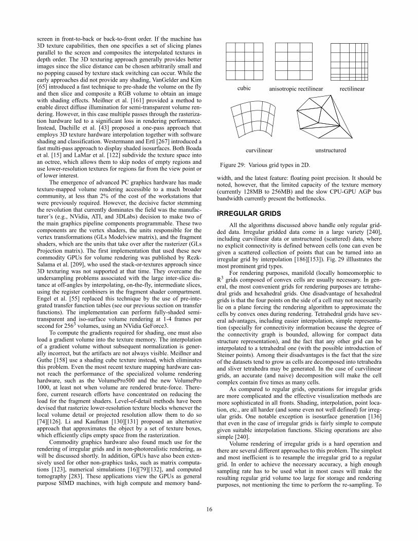
screen in front-to-back or back-to-front order. If the machine has3D texture capabilities, then one specifies a set of slicing planesparallel to the screen and composites the interpolated textures indepth order. The 3D texturing approach generally provides betterimages since the slice distance can be chosen arbitrarily small andno popping caused by texture stack switching can occur. While theearly approaches did not provide any shading, VanGelder and Kim[65] introduced a fast technique to pre-shade the volume on the flyand then slice and composite a RGB volume to obtain an imagewith shading effects. Meißner et al. [161] provided a method toenable direct diffuse illumination for semi-transparent volume ren-dering. However, in this case multiple passes through the rasteriza-tion hardware led to a significant loss in rendering performance.Instead, Dachille et al. [43] proposed a one-pass approach thatemploys 3D texture hardware interpolation together with softwareshading and classification. Westermann and Ertl [267] introduced afast multi-pass approach to display shaded isosurfaces. Both Boadaet al. [15] and LaMar et al. [122] subdivide the texture space intoan octree, which allows them to skip nodes of empty regions anduse lower-resolution textures for regions far from the view point orof lower interest.

The emergence of advanced PC graphics hardware has madetexture-mapped volume rendering accessible to a much broadercommunity, at less than 2% of the cost of the workstations thatwere previously required. However, the decisive factor stemmingthe revolution that currently dominates the field was the manufac-turer’s (e.g., NVidia, ATI, and 3DLabs) decision to make two ofthe main graphics pipeline components programmable. These twocomponents are the vertex shaders, the units responsible for thevertex transformations (GLs Modelview matrix), and the fragmentshaders, which are the units that take over after the rasterizer (GLsProjection matrix). The first implementation that used these newcommodity GPUs for volume rendering was published by Rezk-Salama et al. [209], who used the stack-or-textures approach since3D texturing was not supported at that time. They overcame theundersampling problems associated with the large inter-slice dis-tance at off-angles by interpolating, on-the-fly, intermediate slices,using the register combiners in the fragment shader compartment.Engel et al. [55] replaced this technique by the use of pre-inte-grated transfer function tables (see our previous section on transferfunctions). The implementation can perform fully-shaded semi-transparent and iso-surface volume rendering at 1-4 frames persecond for 2563 volumes, using an NVidia GeForce3.

To compute the gradients required for shading, one must alsoload a gradient volume into the texture memory. The interpolationof a gradient volume without subsequent normalization is gener-ally incorrect, but the artifacts are not always visible. Meißner andGuthe [158] use a shading cube texture instead, which eliminatesthis problem. Even the most recent texture mapping hardware can-not reach the performance of the specialized volume renderinghardware, such as the VolumePro500 and the new VolumePro1000, at least not when volume are rendered brute-force. There-fore, current research efforts have concentrated on reducing theload for the fragment shaders. Level-of-detail methods have beendevised that rasterize lower-resolution texture blocks whenever thelocal volume detail or projected resolution allow them to do so[74][126]. Li and Kaufman [130][131] proposed an alternativeapproach that approximates the object by a set of texture boxes,which efficiently clips empty space from the rasterization.

Commodity graphics hardware also found much use for therendering of irregular grids and in non-photorealistic rendering, aswill be discussed shortly. In addition, GPUs have also been exten-sively used for other non-graphics tasks, such as matrix computa-tions [123], numerical simulations [16][79][132], and computedtomography [283]. These applications view the GPUs as generalpurpose SIMD machines, with high compute and memory band-

width, and the latest feature: floating point precision. It should benoted, however, that the limited capacity of the texture memory(currently 128MB to 256MB) and the slow CPU-GPU AGP busbandwidth currently present the bottlenecks.

IRREGULAR GRIDSAll the algorithms discussed above handle only regular grid-

ded data. Irregular gridded data come in a large variety [240],including curvilinear data or unstructured (scattered) data, whereno explicit connectivity is defined between cells (one can even begiven a scattered collection of points that can be turned into anirregular grid by interpolation [186][153]). Fig. 29 illlustrates themost prominent grid types.

For rendering purposes, manifold (locally homeomorphic toR3 grids composed of convex cells are usually necessary. In gen-eral, the most convenient grids for rendering purposes are tetrahe-dral grids and hexahedral grids. One disadvantage of hexahedralgrids is that the four points on the side of a cell may not necessarilylie on a plane forcing the rendering algorithm to approximate thecells by convex ones during rendering. Tetrahedral grids have sev-eral advantages, including easier interpolation, simple representa-tion (specially for connectivity information because the degree ofthe connectivity graph is bounded, allowing for compact datastructure representation), and the fact that any other grid can beinterpolated to a tetrahedral one (with the possible introduction ofSteiner points). Among their disadvantages is the fact that the sizeof the datasets tend to grow as cells are decomposed into tetrahedraand sliver tetrahedra may be generated. In the case of curvilineargrids, an accurate (and naive) decomposition will make the cellcomplex contain five times as many cells.

As compared to regular grids, operations for irregular gridsare more complicated and the effective visualization methods aremore sophisticated in all fronts. Shading, interpolation, point loca-tion, etc., are all harder (and some even not well defined) for irreg-ular grids. One notable exception is isosurface generation [136]that even in the case of irregular grids is fairly simple to computegiven suitable interpolation functions. Slicing operations are alsosimple [240].

Volume rendering of irregular grids is a hard operation andthere are several different approaches to this problem. The simplestand most inefficient is to resample the irregular grid to a regulargrid. In order to achieve the necessary accuracy, a high enoughsampling rate has to be used what in most cases will make theresulting regular grid volume too large for storage and renderingpurposes, not mentioning the time to perform the re-sampling. To

cubic anisotropic rectilinear rectilinear

curvilinear unstructured

Figure 29: Various grid types in 2D.

16

overcome the need to fix the resolution of the regular grid to thesmallest cell in the irregular grid, one can sample the data into adetail-adaptive octree whose local height is determined by the localgranularity of the grid [126]. The octree decomposition also allowsthe grid to be rendered within a time-critical rendering framework.

One approach for rendering irregular grids is the use of feed-forward (or projection) methods, where the cells are projected ontothe screen one by one, accumulating their contributions incremen-tally to the final image [275][153][273][228]. The projection algo-rithm that has gained popularity is the Projected Tetrahedra (PT)algorithm by Shirley and Tuchman [228]. It uses the projected pro-file of each tetrahedron with respect to the image plane to decom-pose it into a set of triangles. This gives rise to four classes ofprojections, which are shown in Fig. 30. The color and opacity val-ues for each triangle vertex are approximated using ray integrationthrough the thickest point of the tetrahedron. The resulting semi-transparent triangles are sorted in depth order and then renderedand composited using polygonal graphics hardware. Stein et al.[243] sort the cells before they are split into tetrahedra, and theyutilize 2D texture mapping hardware to accelerate opacity interpo-lation and provide the correct per-pixel opacity values to avoid arti-facts. While their method can only handle linear transfer functionswithout artifacts, Röttger et al. [211] introduced the concept of pre-integrated volume rendering to allow for arbitrary transfer func-tions. They create a 3D texture map to provide hardware support ininterpolating along the ray between the front and back faces of atetrahedral cell. In this texture map, two of the three coordinatescorrespond to values at the cell entry and exit points, with the thirdcoordinate mapping to the distance through the cell. This texturemap is then approximated using two-dimensional texture mapping.

Cell projection methods require a sorted list of cells to bepassed to the hardware. Starting with Max et al.’s [153] and Will-iams’s [276] works, there has been substantial progress in thedevelopment of accurate visibility ordering algorithms [232][38].A graphics hardware architecture was also proposed, but not yetrealized, by King et al. [110], which can both rasterize and sort tet-rahedral meshes in hardware.

An alternative technique to visualize irregular grids is by ray-casting [64][260]. Ray-casting methods tend to be more exact thanprojective techniques since they are able to “stab” or integrate thecells in depth order, even in the presence of cycles. This is gener-ally not possible in cell-by-cell projection methods. Many ray-cast-ing approaches employ the plane sweep paradigm, which is basedon processing geometric entities in an order determined by passinga line or a plane over the data. It was pioneered by Giertsen [66] for

the use in volume rendering. It is based on a sweep plane that isorthogonal to the viewing plane (e.g., orthogonal to the y-axis).Events in the sweep are determined by vertices in the dataset andby values of y that correspond to the pixel rows. When the sweepplane passes over a vertex, an "Active Cell List" (ACL) is updatedaccordingly, so that it stores the set of cells currently intersected bythe sweep plane. When the sweep plane reaches a y-value thatdefines the next row of pixels, the current ACL is used to processthat row, casting rays, corresponding to the values of x that deter-mine the pixels in the row, through a regular grid (hash table) thatstores the elements of the ACL. This method has three majoradvantages: It is unnecessary to store explicitly the connectivitybetween the cells; it replaces the relatively expensive operation of3D ray-casting with a simpler 2D regular grid ray-casting; and itexploits coherence of the data between scanlines. Since then, therehas been a number of works that employ the sweep paradigm, mostusing a sweep plane that is parallel to the image plane. Some ofthese methods are assisted by hardware [285][267], while othersare pure-software implementations [22][56][231]. The ZSweep[56] algorithm is very fast and has excellent memory efficiency. Itsweeps the plane from front to back, and rasterizes the cell faces asthey are encountered by the sweep plane. This keeps the memoryfootprint low since only the active cell set has be held in memory.Finally, Hong and Kaufman [85][86] proposed a very fast ray-cast-ing technique, that exploits the special topology of cuvilinear grids.

TIME-VARYING AND HIGH-DIMENSIONAL DATAA significant factor contributing to the growth in the size of

computational science datasets is the fact that the time steps in thesimulations have become increasingly finer in recent years. Therehave been significant developments in the rendering of time-vary-ing volumetric datasets. These typically exploit time-coherency forcompression and acceleration [3][74][141][225][247][266], butother methods have also been designed that allow general viewing[6][13][76][77][78][106][263] of high-dimensional (n-D) datasetsand require a more universal data decomposition.

In n-D viewing, the direct projection from n-D to 2D (for n>3)is challenging. One major issue is that there are an infinite numberof orderings to determine occlusion (for n=3 there are just two, theview from the front and the view from the back). In order to sim-plify the user interface and to eliminate the amount of occlusionexplorations a user has to do, Bajaj et. al. [6] performed the n-Dvolume renderings as an X-ray projection, where ordering is irrele-vant. The authors demonstrated that, despite the lack of depth cues,much useful topological information of the n-D space can berevealed in this way. They also presented a scalable interactive userinterface that allows the user to change the viewpoint into n-Dspace by stretching and rotating a system of n axis vectors.

On the other end of the spectrum are algorithms [13] (and theearlier [263]) that first calculate an n-D hyper-surface (a tetrahedralgrid in 4D) for a specific iso-value, which can then be interactivelysliced along any arbitrary hyperplane to generate an opaque 3Dpolygonal surface for hardware-accelerated view-dependent dis-play. This approach is quite attractive as long as the iso-value iskept constant. However, if the iso-value is modified, a new iso-tet-rahedralization must be generated which can take on the order oftens of minutes [13].

Since 4D datasets can become quite large, a variety of meth-ods to compress 4D volumes were proposed in recent years.Researchers used wavelets [73], DCT-encoding [141], RLE-encod-ing [3], and images [224][225]. All are lossy to a certain degree,depending on a set tolerance. An alternative compression strategyis the use of more efficient sampling grids, such as the BCC grids.Neophytou and Mueller [182] extended these grids for 4D volumerendering and use a 3D hyperslicer to extract 3D volumes for

Class 1

Class 2

Class 3Class 4

Figure 30: The four classes in tetrahedral projection.

17

shaded and semi-transparent volume visualization with occlusionordering.

Early work on 4D rendering includes a paper by Ke and Pan-duranga [106] who used the hyperslice approach to provide viewsonto the on-the-fly computed 4D Mandelbrot set. Another earlywork is a paper by Rossignac [212], who gave a more theoreticaltreatment of the options available for the rendering of 4D hyper-solids generated, for example, by time-animated or colliding 3Dsolids. Hanson et al. [76][77][78] wrote a series of papers that use4D lighting in conjunction with a technique that augments 4Dobjects with renderable primitives to enable direct 4D renderings.The images they provided in [77] are somewhat reminiscent toobjects rendered with motion blur. The 4D isosurface algorithmsproposed by Weigle and Banks [263] and Bhaniramka, Wenger,and Crawfis [13] both use a Marching Cubes-type approach andgeneralize it into n-D.

Methods that focus more on the rendering of the time-variantaspects of 3D datasets have stressed the issue of compression andtime-coherence to facilitate interactive rendering speeds. Shen andJohnson [226] used difference encoding of time-variant volumes toreduce storage and rendering time. Westermann [266] used a wave-let decomposition to generate a multi-scale representation of thevolume. Shen, Chiang, and Ma [225] proposed the Time-SpacePartitioning (TSP) tree, which allows the renderer to cache and re-use partial (node) images of volume portions static over a timeinterval. It also enables the renderer to use data from sub-volumesat different spatial and temporal resolutions. Anagnostou [3]extended the RLE data encoding of the shear-warp algorithm [120]into 4D, inserting a new run block into the data-structure whenevera change is detected over time. They then composited the renderedrun block with partial rays of temporally-unchanged volume por-tions. Sutton and Hansen [247] expanded the Branch-On-NeedOctree (BONO) approach of Wilhelms and Van Gelder [274] totime-variant data to enable fast out-of-core rendering of time-vari-ant isosurfaces. Lum, Ma, and Clyne [141] advocated an algorithmthat DCT-compresses time-runs of voxels into single scalars thatare stored in a texture map. These texture maps, one per volumeslice, are loaded into a texture-map accelerated graphics board.Then, during time-animated rendering, the texture maps areindexed by a time-varying color palette that relates the scalars inthe texture map to the current color of the voxel they represent.Although the DCT affords only a lossy compression, their render-ing results are quite good and can be produced interactively.Another compression-based algorithm was proposed by Guthe andStraßer [74], who used a lossy MPEG-like approach to encode thetime-variant data. The data were then decompressed on-the-fly fordisplay with texture mapping hardware.

MULTI-CHANNEL AND MULTI-MODAL DATASo far, we have assumed that a voxel had a scalar density

value from which other multi-variate properties could be derived,for example, via transfer function lookup. We shall now extend thisnotion to datasets where the voxel data come originally in form ofmulti-variate vectors. In the context of this discussion, we shalldistinguish between vectors of physical quantities, such as flowand strain, and vectors that store a list of voxel attributes. There is alarge body of literature to visualize the former, including line inte-gral convolution [23], spot noise [272], streamlines and stream-balls [21], glyphs, texture splats [42], and many more. In thissection, we shall focus on the latter scenario, that is, volumes com-posed of attribute vectors. These can be (i) multi-channel, such asthe RGB color volumes obtained by cryosectioning the VisibleHuman [91] or multi-spectra remote sensing satellite data, or (ii)multi-modal, that is, volumes acquired by scanning an object withmultiple modalities, such as MRI, PET, and CT.

The rendering of multi-modal volumes requires the mixing ofthe data at some point in the rendering pipeline. There are at leastthree locations at which this can happen [25]. For the followingdiscussion, let us assume a set of two co-located volumes, but thisis not a limitation. The simplest mixing technique is image-levelintermixing, i.e., to render each volume separately as a scalardataset and then blend the two images according to some weight-ing function that possibly includes the z-buffer or opacity channel(see Fig a). This method is attractive since it does not require amodification of the volume renderer, but as Fig. 32a (top) shows, itgives results of limited practical value since depth ordering is notpreserved. This can be fixed by intermixing the rendering results atevery step along the ray, which gives rise to accumulation levelintermixing. Here, we assign separate colors and opacities for eachvolume’s ray sample, and then combine these according to somemixing function (see Fig. 32a (bottom)). A third method is illumi-nation model level intermixing, where one combines the ray sam-ples before colors and opacities are computed. One could just use aweighted sum of the two densities to look up opacities and colors,or one could have one of the volumes act as an emission volumeand the other as an attenuation volume. This would work quite nat-urally, for example, for the visualization of the emissive metabolicactivities in a SPECT volume within the spatial context of a CTattenuation volume. Cai and Sakas [25] demonstrate this method inthe scenario of dose planning in radiation therapy, where they visu-alize an (emissive) radiation beam embedded in an (attenuating)CT volume.

Multi-channel data, such as RGB data obtained by ways ofphotographing slices of real volumetric objects, have the advantagethat there is no longer a need to search for suitable color transferfunctions to reproduce the original look of the data. On the otherhand, the photographic data do not provide an easy mapping todensities and opacities, which are required to compute normals andother parameters needed to bring out structural object detail in sur-face-sensitive rendering. One can overcome the perceptional non-linearities of the RGB space by computing gradients and higherderivatives in the perceptionally uniform color space L*u*v* [51].In this method, the RGB data are first converted into the L*u*v*space, and the color distance between two voxels is calculated by

Traversing

Sampling and Interpolation

Illumination

Accumulation

image-level

accumulation-level

illumination model level intermixing intermixing

intermixing

volume1volume 2

Figure 31: Levels in the volume rendering pipeline at whichdata mixing can occur.

mixed volume

18

their Euclidian distance in that color space. A gradient can then becalculated as usual via central differences, but replacing the voxeldensities by the color distances. Although one cannot determinethe direction of the normal vector with this method, this is not alimiting factor in practice. One can also derive more descriptivequantities, such as tensor gradients, since we are now dealing withvectors and not with densities in the gradient calculation. Thesecan be used for segmentation, texture analysis, and others. Finally,opacities can be computed by using different functions of higher-level gradients to bring out different textural and structural aspectsof the data [172].

NON-PHOTOREALISTIC VOLUME RENDERINGNon-photorealistic volume rendering (NPVR) is a relatively

recent branch of volume rendering. It employs local image pro-cessing during the rendering to produce artistic and illustrativeeffects, such as feature halos, tone shading, distance color blend-ing, stylized motion blur, boundary enhancements, fading, silhou-ettes, sketch lines, stipple patterns, and pen+ink drawings[52][53][137][138][95][140][139][244][257]. The overall goal ofNPVR is to go beyond the means of photo-realistic volume render-ing and produce images that emphasize critical features in the data,such as edges, boundaries, depth, and detail, to provide the user abetter appreciation of the structures in the data. This is similar tothe goals of medical and other illustrators, as well as related effortsin general computer graphics [277][278][216][217]. Since the setof parameters that can be tuned in NPVR is even larger than fortraditional volume rendering, interactive rendering of the NPVReffects is crucial, and indeed a number or researchers have pro-posed interactive implementations that exploit the latest genera-tions of commodity programmable graphics hardware [139][244].

REFERENCES[1] J. Amanatides, and A. Woo, “A Fast Voxel Traversal Algo-

rithm for Ray Tracing,” Eurographics'87, 1987.[2] M. Amin, A. Grama, V. Singh, “Fast Volume Rendering

Using an Efficient, Scalable Parallel Formulation of theShear-Warp Algorithm”, Proc. Parallel Rendering Sympo-sium’95, pp. 7-14, 1995.

[3] K. Anagnostou, T. Atherton, and A. Waterfall, “4D volumerendering with the Shear Warp factorization,” Symp. VolumeVisualization and Graphics’00, pp. 129-137, 2000.

[4] R. Avila, L. Sobierajski, and A. Kaufman, “Towards a Com-prehensive Volume Visualization System”, Proc. of IEEEVisualization '92, pp. 13-20, 1992.

[5] R. Avila, T. He, L. Hong, A. Kaufman, H. Pfister, C. Silva, L.Sobierajski, and S. Wang, “VolVis: A Diversified System forVolume Visualization,” Proc. of IEEE Visualization'94,1994.

[6] C. Bajaj, V. Pascucci, and D. Schikore, “The contour spec-trum,” Proc. IEEE Visualization’97, pp. 167-175, 1997.

[7] C. Bajaj, V. Pascucci, G. Rabbiolo, and D. Schikore, “Hyper-volume visualization: A challenge in simplicity,” Proc. 1998Symposium on Volume Visualization’98, pp. 95-102, 1998.

[8] R. Bakalash, A. Kaufman, R. Pacheco, and H. Pfister, “AnExtended Volume Visualization System for Arbitrary parallel

(a)

(b)

(c)

Figure 32: Multi-modal rendering with data intermixing: (a) One time step of a time-varying volume (magenta) and vol-ume motion-blurred across 10 time steps (blue). (top): image-level intermixing, (bottom): accumulation-level intermixing[182].(b) Accumulation-level intermixing of the Visible Man’s CTand a MRI dataset. Here we assign blue of CT>MRI and greenif MRI>CT. (left): gradients specified on CT while MRI is ren-dered as a point cloud; (right): surfaces rendered with gradientmodulation [70].(c) Accumulation-level intermixing of the Visible Man’s CTand a MRI dataset, rendered in inclusive opacity mode,i.e., . (left) unweighted productof CT and MRI, (right) more CT than MRI [70].

α 1 1 αCT–( ) 1 αMRI–( )–=Figure 33: Rendering of multi-channel (photographic) data.(a) The L* component (related to brightness); (b) The u* com-ponent (related to the chromatic change in red-green colors);(c) Color difference gradient computed in RGB color space;(b) Gradients computed in L*u*v* space, using the secondderivative along the gradient direction to compute opacity.(Images from [70]).

(a)

(d)(c)

(b)

19

Projection,” Proc. of Eurographics Workshop on GraphicsHardware’92, 1992.

[9] D. Banks, and B. Singer, “Vortex tubes in turbulent flows;identification, representation reconstruction,” Proc. of IEEEVisualization’94, pp. 132-139, 1994.

[10] D. Bauer, and R. Peikert, “Vortex Tracking in Scale-Space,”Joint EUROGRAPHICS - IEEE TCVG Symposium on Visual-ization (2002), VisSym'02, 2002.

[11] M. Bentum, B.B.A. Lichtenbelt, and T. Malzbender, “Fre-quency analysis of gradient estimators in volume rendering,”IEEE Trans. on Visualization and Computer Graphics’96,vol. 2, no. 3, pp. 242-254, 1996.

[12] S. Bergner, T. Möller, M. Drew, and G. Finlayson, “Interac-tive Spectral Volume Rendering”, Proc. of IEEEVisualization’02, pp. 101-108, 2002.

[13] P. Bhaniramka, R. Wenger, and R. Crawfis, “Isosurfacing inhigher dimensions,” Proc. of IEEE Visualization’00, pp. 267-273, 2000.

[14] F. Blinn, “Light reflection functions for simulation of cloudsand dusty surfaces,” Proc. of SIGGRAPH ’82, pp. 21-29,1982.

[15] I. Boada, I. Navazo, and R. Scopigno, “Multiresolution vol-ume visualization with a texture-based octree,” The VisualComputer, vol. 17, no. 3, pp. 185-197, 2001.

[16] J. Bolz, I. Farmer, E. Grinspun, and P. Schröder, “The GPUas numerical simulation engine,” SIGGRAH’03, 2003.

[17] R. Bracewell, The Fourier Transform and its Applications-3rd edition, McGraw-Hill, 1999.

[18] M. Brady, K. Jung, H. Nguyen, and T. Nguyen, “InteractiveVolume Navigation,” IEEE Transactions on Visualizationand Computer Graphics vol. 4, no. 3, pp. 243-256, 1998.

[19] M. Brady, K. Jung, H. Nguyen, and T. Nguyen, “Two-PhasePerspective Ray Casting for InteractiveVolume Navigation,”Visualization ’97, pp. 183–189, 1997.

[20] M. Brady, W. Higgins, K. Ramaswamy, and R. Srinivasan,"Interactive Navigation inside 3D radiological Images," Proc.of BioMedical Visualization’99, Proc. of IEEE Visualiza-tion’99, pp. 33-40 and p. 85 (color plate), 1995.

[21] M. Brill, V. Djatschin, H. Hagen, S. V. Klimenko, and H.-C.Rodrian, “Streamball techniques for flow visualization,”Proc. of IEEE Visualization '94, pp. 225-231, 1994.

[22] P. Bunyk, A. Kaufman, and C. Silva, “Simple, fast, androbust ray casting of irregular grids,” Scientific Visualization,pp. 30-36, 1997.

[23] B. Cabral, and L. Leedon, “Imaging vector fields using lineintegral convolution,” Proc. of SIGGRAPH '93, pp. 263-272,1993.

[24] B. Cabral, N. Cam, and J. Foran, “Accelerated volume ren-dering and tomographic reconstruction using texture mappinghardware”, Symp. on Volume Visualization’94, pp. 91-98,1994.

[25] W. Cai, and G. Sakas, “Data intermixing and multi-volumerendering,” Computer Graphics Forum, (Eurographics’99),vol. 18, no. 3, 1999.

[26] H. Carr, J. Snoeyink, and U. Axen, “Computing contour treesin all dimensions,” Computational Geometry Theory andApplications’02, vol. 24, no. 2, pp. 75–94, 2003.

[27] J. Challinger, “Scalable Parallel Volume Raycasting forNonrectilinear Computational Grids,” Proc. of Parallel Ren-dering Symposium’93, pp. 81-88, 1993.

[28] B. Chen, A. Kaufman, and Q. Tang, “Image-based renderingof surfaces from volume data,” Workshop on Volume Graph-ics’01, pp. 279-295, 2001.

[29] E. Chen, “QuickTime VR-An Image-Based Approach ToVirtual Environment Navigation,” Proc. of SIGGRAPH ‘95,pp. 29-38, 1995.

[30] E. Chen, and L. Williams, “View Interpolation For ImageSynthesis,” Proc. of SIGGRAPH ‘93, pp. 279-288, 1993.

[31] M. Chen, A. Kaufman, and R. Yagel (Eds.) Volume Graphics,Springer, London, February, 2000.

[32] K. Chidlow, and T. Möller, “Rapid emission volume recon-struction,” (to appear) Volume Graphics Workshop’03, 2003.

[33] T. Chiueh, T. He, A. Kaufman, and H. Pfister, “CompressionDomain Volume Rendering,” Tech. Rep. 94.01.04, Computerscience, SUNY Stony Brook, 1994.

[34] C. Chui, An Introduction To Wavelets, Academic Press, 1992.[35] P. Cignoni, C. Montani, E. Puppo, and R. Scopigno, “Optimal

isosurface extraction from irregular volume data,” Sym-posium on Volume visualization’96, pp.31-38, 1996.

[36] H. Cline, W. Lorensen, S. Ludke, C. Crawford, and B. Teeter,“Two Algorithms for the Three-Dimensional Reconstructionof Tomograms,” Med. Phys., vol. 15, pp. 320-327, 1988.

[37] D. Cohen, and Z. Shefer, “Proximity clouds - an accelerationtechnique for 3D grid traversal,” The Visual Computer, vol.10, no. 11, pp. 27-38, 1994.

[38] J. Comba, J. Klosowski, N. Max, J. Mitchell, C. Silva, and PWilliams, “Fast polyhedral cell sorting for interactive render-ing of unstructured grids,” Computer Graphics Forum, vol.18, no. 3, pp. 369-376, 1999.

[39] J. Conway, and N. Sloane, Sphere Packings, Lattices andGroups, Springer Verlag, 2nd edition, 1993.

[40] B. Corrie, and P. Mackerras, “Parallel Volume Rendering andData Coherence”, Proc. of Parallel Rendering Sympo-sium’93, pp. 23-26, 1993.

[41] R. Crawfis, “Real-time Slicing of Data Space,” Proc. of IEEEVisualization'96, pp. 271-277, 1996.

[42] R. Crawfis, and N. Max, “Texture splats for 3D scalar andvector field visualization,” Proc. of IEEE Visualization’93,pp. 261-266, 1993.

[43] F. Dachille, K. Kreeger, B. Chen, I. Bitter, and A. Kaufman,“High-Quality Volume Rendering Using Texture MappingHardware,” SIGGRAPH/Eurographics Workshop on Graph-ics Hardware’98, 1998.

[44] F. Dachille, K. Mueller, and A. Kaufman, “Volumetric Back-projection,” Volume Visualization Symposium’00, pp. 109-117, 2000.

[45] J. Danskin, and P. Hanrahan, “Fast algorithms for volume raytracing,” Workshop on Volume Visualization, pp. 91-98,1992.

[46] I. Daubechies, “Ten Lectures on Wavelets,” CBMS-NSF Reg.Conf. Ser. Appl. Math. SIAM. 1992.

[47] J. Dorsey, A. Edelman, H. Jensen, J. Legakis, and H. Peder-son, “Modeling and rendering of weathered stone,” Proc. ofSIGGRAPH '99, pp. 225-234, 1999.

[48] R. Drebin, L. Carpenter and P. Hanrahan, “Volume Render-ing,” Proc. of SIGGRAPH’88, vol. 22, no. 4, pp. 65-74, 1988.

[49] D. Dudgeon, and R. Mersereau, Multi-dimensional DigitalSignal Processing, Prentice-Hall: Englewood Cliffs, 1984.

[50] S. Dunne, S. Napel, and B. Rutt, “Fast reprojection of volumedata,” Proc. of IEEE Visualization in Biomed. Comput, pp.11-18, 1990.

[51] D. Ebert, C. Morris, P. Rheingans, and T. Yoo, “Designingeffective transfer functions for volume rendering from photo-graphics volumes,” IEEE Trans. on Visualization andComputer 3Graphics, vol. 8, no. 2, pp. 183-197, 2002.

[52] D. Ebert, and P. Rheingans, “Volume Illustration: Non-Pho-torealistic Rendering of Volume Models,” IEEE Transactionson Visualization and Computer Graphics, vol. 7, no. 3, pp.253-265, 2001.

[53] D. Ebert, and P. Rheingans, “Volume Illustration: Non-Pho-torealistic Rendering of Volume Models,” Proc. of IEEEVisualization’00, pp. 195-202, 2000.

20

[54] T. Elvins, “Volume Rendering on a Distributed Memory Par-allel Computer”, Proc. of Parallel Rendering Symposium’93,pp. 93-98, 1993.

[55] K. Engel, M. Kraus, and T. Ertl, “High-Quality Pre-IntegratedVolume Rendering Using Hardware-Accelerated Pixel Shad-ing,” Proc. of SIGGRAPH Graphics Hardware Workshop’01,pp. 9-16, 2001.

[56] R. Farias, J. Mitchell, and C. Silva, “ZSWEEP: An Efficientand Exact Projection Algorithm for Unstructured VolumeRendering,” ACM/IEEE Volume Visualization and GraphicsSymposium, pp. 91-99, 2000.

[57] J. Foley, A. Dam, S. Feiner, and J. Hughes, Computer Graph-ics: Principles and Practice. Addison-Wesley, 2nd edition,1996.

[58] J. Fowler, and R. Yagel, “Lossless compression of volumedata,” Symp. of Volume Visualization’94, pp. 43-50, 1994.

[59] A. Fujimoto, T. Tanaka, and K. Iwata, “ARTS: acceleratedray-tracing system,” IEEE Computer Graphics and Applica-tions, vol. 6, no. 4, pp. 16-26, 1986.

[60] I. Fujishiro, Y. Takeshima, T. Azuma, and S. Takahashi,“Volume Data Mining Using 3D Field Topology Analysis,”IEEE Computer Graphics & Applications, vol. 20, no. 5, pp.46-51, 2000.

[61] A. Gaddipati, R. Machiraju, and R. Yagel, "Steering Imagegeneration using Wavelet Based Perceptual Metric," Com-puter Graphics Forum (Proc. of Eurographics `97), vol. 16,no. 3, pp. 241-251, 1997.

[62] J. Gao, and H. Shen, “Parallel View-Dependent IsosurfaceExtraction Using Multi-Pass Occlusion Culling,” ACM/IEEESymposium on Parallel and Large Data Visualization andGraphics, 2001.

[63] M. Garland, and P. Heckbert, “Surface simplification usingquadric error metrics,” Proc. of the 24th annual conferenceon Computer graphics and interactive techniques, pp.209-216, 1997.

[64] M. Garrity, “Raytracing irregular volume data,” ComputerGraphics, pp. 35-40, November 1990.

[65] V. Gelder, and K. Kim, “Direct volume rendering via 3D tex-ture mapping hardware,” Proc. of Vol. Rend. Symp.’96, pp.23-30, 1996.

[66] C. Giertsen, “Volume visualization of sparse irregularmeshes,” IEEE Computer Graphics and Applications, vol.12, no.2, pp. 40-48, March 1992.

[67] S. Goldwasser, R. Reynolds, T. Bapty, D. Baraff, J. Summers,D. Talton, and E. Walsh, “Physician’s Workstation withReal-Time Performance,” IEEE Computer Graphics & Appli-cations, vol. 5, no. 12, pp. 44-57, 1985.

[68] D. Gordon and R. Reynolds, “Image-space shading of 3-dimensional objects,“ Computer Vision, Graphics, and ImageProcessing, 29, pp. 361-376, 1985.

[69] S. Gortler, R. Grzeszczuk, R. Szeliski, and M. Cohen, “TheLumigraph,” Proc. of SIGGRAPH ‘96, pp. 43-54, 1996.

[70] A. Gosh, P. Prabhu, A. Kaufman, and K. Mueller, “HardwareAssisted Multichannel Volume Rendering,” (to be presented)Computer Graphics International’03, 2003.

[71] M. Gross, R. Koch, L. Lippert, and A. Dreger, “A newmethod to approximate the volume rendering equation usingwavelet bases and piecewise polynomials,” Computers &Graphics, vol. 19 no. 1, pp.47-62, 1995.

[72] T. Guenther, C. Poliwoda, C. Reinhard, J. Hesser, R. Maen-ner, H. Meinzer, and H. Baur, “VIRIM: A Massively ParallelProcessor for Real-Time Volume Visualization in Medicine,”Proc. of the 9th Eurographics Hardware Workshop, pp. 103-108, 1994.

[73] S. Guthe, M. Wand, J. Gonser, and W. Strasser, “Interactiverendering of large volume datasets,” Proc. of IEEE Visualiza-

tion’02, pp. 53-60, 2002.[74] S. Guthe, and W. Straßer, “Real-time decompression and

visualization of animated volume data,” Proc. of IEEE Visu-alization’01, 2001.

[75] P. Hanrahan, and W. Krueger, “Reflection from layered sur-faces due to subsurface scattering,” Computer Graphics(Proc. of SIGGRAPH’93), pp. 165-174, 1993.

[76] A. Hanson, and P. Heng, “Four-dimensional views of 3D sca-lar fields,” Proc. of IEEE Visualization’92, pp. 84-91, 1992.

[77] A. Hanson, and P. Heng, “Illuminating the fourth dimension,”IEEE Computer Graphics & Applications, vol. 12, no. 4, pp.54-62, 1992.

[78] A. Hanson, and R. Cross, “Interactive visualization methodsfor four dimensions,” Proc. of IEEE Visualization’93, pp.196-203, 1993.

[79] M. Harris, G. Coombe, T. Scheuermann, and A. Lastra,“Physically-Based Visual Simulation on Graphics Hard-ware,” Proc. of 2002 SIGGRAPH/Eurographics Workshopon Graphics Hardware, 2002.

[80] H. Hauser, L. Mroz, G. Bischi, and M. Gröller, “Two-levelvolume rendering-flushing MIP and DVR,” Proc. of IEEEVisualization’00, pp. 211-218, 2000.

[81] T. He, L. Hong, A. Kaufman, and H. Pfister, “Generation ofTransfer Functions with Stochastic Search Techniques,”Proc. of IEEE Visualization’96, pp. 227-234, 1996.

[82] G. Herman, and H. Liu, “Three-dimensional display ofhuman organs from computed tomograms,” Comput. Graph-ics Image Process, vol. 9, pp. 1-21, 1979.

[83] G. Herman and J. Udupa, “Display of three-dimensional dis-crete surfaces,“ Proceedings SPIE, 283, pp. 90-97, 1981.

[84] J. Hesser, R. Maenner, G. Knittel, W. Strasser, H. Pfister, andA. Kaufman, “Three Architectures for Volume Rendering,”Computer Graphics Forum, vol. 14, no. 3, pp. 111-122, 1995.

[85] L. Hong, and A. Kaufman, “Accelerated ray-casting forcurvilinear volumes,” Proc. of IEEE Visualization’98, pp.247-253, 1998.

[86] L. Hong, and A. Kaufman, “Fast Projection-Based Ray-Cast-ing Algorithm for Rendering Curvilinear Volumes,” IEEETransactions on Visualization and Computer Graphics vol. 5,no. 4, pp. 322-332, 1999.

[87] L. Hong, S. Muraki, A. Kaufman, D. Bartz, and T. He, “Vir-tual Voyage: Interactive Navigation in the Human Colon,”Proc. of ACM SIGGRAPH’97, pp. 27-34, August 1997.

[88] H. Hoppe, “Progressive Meshes,” Proc. of SIGGRAPH’96,pp. 99-108, 1996.

[89] W. Hsu, “Segmented Ray Casting for Data Parallel VolumeRendering”, Proc. of Parallel Rendering Symposium’93, pp.93-98, 1993.

[90] http://graphics.stanford.edu/software/volpack/[91] http://www.nlm.nih.gov/research/visible/

visible_human.html[92] J. Huang, N. Shareef, R. Crawfis, P. Sadayappan, and K.

Mueller, “A Parallel Splatting Algorithm with OcclusionCulling,” 3rd Eurographics Workshop on Parallel Graphicsand Visualization, 2000.

[93] J. Huang, R. Crawfis, and D. Stredney, “Edge preservation involume rendering using splatting,” IEEE Volume Vis.’98, pp.63-69, 1998.

[94] I. Ihm, and R. Lee, “On enhancing the speed of splatting withindexing,” Proc. of IEEE Visualization '95, pp. 69-76, Octo-ber 1995.

[95] V. Interrante, “Illustrating surface shape in volume data viaprincipal direction-driven 3D line integral convolution,”Proc. of SIGGRAPH’97, pp. 109-116, August, 1997.

[96] D. Jackel, “The Graphics PARCUM System: A 3D MemoryBased Computer Architecture for Processing and Display of

21

Solid Models,” Computer Graphics Forum, vol. 4, pp. 21-32,1985.

[97] H. Jensen, and P. Christensen, “Efficient Simulation of LightTransport in Sciences with Participating Media Using PhotonMaps,” Proc. of SIGGRAPH’98, pp. 311-320, 1998.

[98] J. Kajiya, and B. Herzen, “Ray tracing volume densities,”Proc. of SIGGRAPH‘84, pp. 165-174, 1994.

[99] K. Kaneda, Y. Dobashi, K. Yamamoto, and H. Yamashita,“Fast volume rendering with adjustable color maps,” 1996Symposium on Volume Visualization, pp. 7-14, 1996.

[100] A. Kaufman, Volume Visualization, IEEE Computer SocietyPress Tutorial, Los Alamitos, CA.

[101] A. Kaufman, “Volume visualization,” ACM Computing Sur-veys, 28, 1 pp. 165-167, 1996.

[102] A. Kaufman, and R. Bakalash, “CUBE - An ArchitectureBased on a 3-D Voxel Map,” Theoretical Foundations ofComputer Graphics and CAD, R. A. Earnshaw (ed.),Springer-Verlag, pp. 689-701, 1985.

[103] A. Kaufman, and R. Bakalash, “Memory and ProcessingArchitecture for 3-D Voxel-Based Imagery,” IEEE ComputerGraphics & Applications, vol. 8, no. 6, pp. 10-23, 1988. Alsoin Japanese, Nikkei Computer Graphics, vol. 3, no. 30, pp.148-160, 1989.

[104] A. Kaufman, D. Cohen, and R. Yagel, “Volume graphics,”IEEE Computer, vol. 26, no. 7, pp. 51-64, 1993.

[105] T. Kay, and J. Kajiya, “Ray Tracing Complex Scenes,” Proc.of SIGGRAPH’86, p269-278, 1986.

[106] Y. Ke, and E. Panduranga, “A journey into the fourth dimen-sion,” Proc. of IEEE Visualization’89, pp. 219-229, 1989.

[107] R. Keys, “Cubic convolution interpolation for digital imageprocessing,” IEEE Transactions. on Acoustics, Speech, Sig-nal Processing, vol. 29, no. 6, pp. 1153-1160, 1981.

[108] S. Kilthau, and T. Möller, "Splatting Optimizations", Techni-cal Report, School of Computing Science, Simon FraserUniversity, (SFU-CMPT-04/01-TR2001-02), April 2001.

[109] G. Kindlmann, and J. Durkin, “Semi-automatic generation oftransfer functions for direct volume rendering,” Symp. Vol-ume Visualization’98, pp. 79-86, 1998.

[110] D. King, C. Wittenbrink, and H. Wolters, “An Architecturefor Interactive Tetrahedral Volume Rendering,” InternationalWorkshop on Volume Rendering’01, 2001.

[111] J. Kniss, G. Kindlmann, and C. Hansen, “Interactive volumerendering using multidimensional transfer functions anddirect manipulation widgets,” Proc. of IEEE Visualiza-tion’01, pp. 255-262, 2001.

[112] J. Kniss, G. Kindlmann, and C. Hansen, “MultidimensionalTransfer Functions for Interactive Volume Rendering,” IEEETransactions on Visualization and Computer Graphics, vol.8, no. 3, pp. 270-285, 2002.

[113] J. Kniss, S. Premoze, C. Hansen, P. Shirley, and A. McPher-son, “Interactive Volume Light Transport and ProceduralModeling,” IEEE Transactions on Visualization and Com-puter Graphics, 2003.

[114] J. Kniss, S. Premoze, C. Hansen, and D. Ebert, “InteractiveTranslucent Volume Rendering and Procedural Modeling,”Proc. of IEEE Visualization’02, pp. 109-116, 2002.

[115] G. Knittel, “The ULTRAVIS system,” Proc. of Volume Visu-alization and Graphics Symposium’00, pp. 71-80, 2000.

[116] G. Knittel, and W. Strasser, “A Compact Volume RenderingAccelerator,” Volume Visualization Symposium Proceedings,pp. 67-74, 1994.

[117] K. Kreeger, and A. Kaufman, “Interactive Volume Segmen-tation with the PAVLOV Architecture,” Proc. of ParallelVisualization and Graphics Symposium’99, 1999.

[118] K. Kreeger, I. Bitter, F. Dachille, B. Chen, and A. Kaufman,“Adaptive Perspective Ray Casting,” Volume Visualization

Symposium’98, pp. 55-62. 1998[119] M. Kreveld, R. Oostrum, C. Bajaj, V. Pascucci, and D.

Schikore, “Contour Trees and Small Seed Sets for IsosurfaceTraversal,” Proc. of the 13th ACM Symposium on Computa-tional Geometry, pp. 212-220, 1997.

[120] P. Lacroute, and M. Levoy, “Fast volume rendering using ashear-warp factorization of the viewing transformation,”Proc. of SIGGRAPH ‘94, pp. 451-458, 1994.

[121] P. Lacroute, “Analysis of a Parallel Volume Rendering Sys-tem Based on the Shear-Warp Factorization”, IEEE Trans. ofVisualization and Computer Graphics, vol. 2, no. 3, pp. 218-231, 1996.

[122] E. LaMar, B. Hamann, and K. Joy, “Multiresolution Tech-niques for Interactive Texture-Based Volume Visualization,”Proc. of IEEE Visualization’99, pp. 355-361, 1999.

[123] E. Larsen, and D. McAllister, “Fast Matrix Multiplies usingGraphics Hardware,” Supercomputing’01, 2001.

[124] D. Laur, and P. Hanrahan, “Hierarchical splatting: A progres-sive refinement algorithm for volume rendering,” Proc. ofSIGGRAPH’91, pp. 285-288, 1991.

[125] R. Lee, and I. Ihm, “On enhancing the speed of splatting usingboth object- and image space coherence,” Graphical Modelsand Image Processing, vol. 62, no. 4, pp 263-282, 2000.

[126] J. Leven, J. Corso, S. Kumar and J. Cohen, “Interactive visu-alization of unstructured grids using hierarchical 3Dtextures,” Proc. of Symposium on Volume Visualization andGraphics’02, pp 33-40, 2002.

[127] M. Levoy, “Display of surfaces from volume data,” IEEEComp. Graph. & Appl., vol. 8, no. 5, pp. 29-37, 1988.

[128] M. Levoy, “Efficient ray tracing of volume data,” ACMTrans. Comp. Graph., vol. 9, no. 3, pp. 245-261, 1990.

[129] M. Levoy, and P. Hanrahan, “Light field rendering,” Proc. ofSIGGRAPH '96, pp. 31-42, 1996.

[130] W. Li, and A. Kaufman, “Accelerating Volume Renderingwith Texture Hulls,” IEEE/Siggraph Symposium on VolumeVisualization and Graphics 2002 (VolVis'02), pp. 115-122,2002.

[131] W. Li, and A. Kaufman, “Texture Partitioning and Packingfor Accelerating Texture-based Volume Rendering,” Graph-ics Interface’03, 2003.

[132] W. Li, X. Wei, and A. Kaufman, “Implementing Lattice Bolt-zmann computation on graphics hardware,” (to appear) TheVisual Computer, 2003.

[133] P. Li, S. Whitman., R. Mendoza, and J. Tsiao, “Prefix - A Par-allel Splattting Volume Rendering System for DistributedVisualization,” Proc. of Parallel Rendering Symposium’97,1997.

[134] B. Lichtenbelt, R. Crane, and S. Naqvi, Volume Rendering,Prentice-Hall, 1998.

[135] Y. Livnat, H. Shen, and C. Johnson, “A near optimal isos-urface extraction algorithm for structured and unstructuredgrids,” IEEE Trans. on Vis. and Comp. Graph. Vol. 2, no. 1,pp. 73-84, 1996.

[136] E. Lorensen, and H. Cline, “Marching cubes: a high resolu-tion 3D surface construction algorithm,” Proc. ofSIGGRAPH’87, pp. 163-169, 1987.

[137] A. Lu, C. Morris, D. Ebert, P. Rheingans, and C. Hansen,“Non-Photorealistic Volume Rendering Using StipplingTechniques,” Proc. of IEEE Visualization’02, pp. 211-217,2002.

[138] A. Lu, C. Morris, J. Taylor, D. Ebert, P. Rheingans, C.Hansen, and M. Hartner, “Illustrative Interactive Stipple Ren-dering,” IEEE Transactions on Visualization and ComputerGraphics, 2003.

[139] E. Lum, and K. Ma, “Hardware-Accelerated Parallel Non-Photorealistic Volume Rendering,” International Symposium

22

on Nonphotorealistic Rendering and Animation’02, 2002.[140] E. Lum, and K. Ma, “Nonphotorealistic Rendering using

Watercolor Inspired Textures and Illumination,” PacificGraphics’01, 2001

[141] E. Lum, K. Ma, and J. Clyne, “Texture hardware assisted ren-dering of time-varying volume data,” Proc. of IEEEVisualization’01, pp. 262-270, 2001.

[142] F. Ma, W. Wang, W. Tsang, Z. Tang, and S. Xia, “Probabilis-tic Segmentation of Volume Data for Visualization UsingSOM-PNN Classifier”, Symposium on Volume Visualiza-tion’98, pp. 71-78, 1998.

[143] K. Ma, and S. Parker, “Massively parallel software renderingfor visualizing large-scale datasets,” IEEE Computer Graph-ics & Applications, pp. 72-83, 2001.

[144] K. Ma., “Parallel Volume Ray-Casting for Unstructured-GridData on Distributed-Memory Architectures”, Proc. of Paral-lel Rendering Symposium’95, pp. 23-30, 1995.

[145] K. Ma, and T. Crockett, “A Scalable Parallel Cell-ProjectionVolume Rendering Algorithm for Three-DimensionalUnstructured Data”, Proc. of Parallel Rendering Sympo-sium’97, 1997.

[146] R. Machiraju, A. Gaddipati, and R. Yagel, “Detection andenhancement of scale cohererent structures using wavelettransform products,” Proc. of the Technical Conference onWavelets in Signal and Image Processing V, SPIE AnnualMeeting, pp. 458-469, 1997.

[147] R. Machiraju, and R. Yagel, “Efficient Feed-Forward Vol-ume Rendering Techniques for Vector and ParallelProcessors,” SUPERCOMPUTING’93, pp. 699-708, 1993.

[148] R. Machiraju, and R. Yagel, “Reconstruction Error and Con-trol: A Sampling Theory Approach,” IEEE Transactions onVisualization and Graphics, vol. 2, no. 3, December 1996.

[149] T. Malzbender, and F. Kitson, “A Fourier Technique for Vol-ume Rendering,” Focus on Scientific Visualization, pp. 305-316, 1991.

[150] J. Marks, B. Andalman, P.A. Beardsley, W. Freeman, S. Gib-son, J. Hodgins, T. Kang, B. Mirtich, H. Pfister, W. Rum,et.al, “Design Galleries: A General Approach to SettingParameters for Computer Graphics and Animation,” Proc. ofSIGGRAPH’97, pp. 389-400, 1997.

[151] S. Marschner, and R. Lobb, “An evaluation of reconstructionfilters for volume rendering,” Proc. of IEEE Visualization’94,pp. 100-107, 1994.

[152] N. Max, “Optical models for direct volume rendering,” IEEETrans. Vis. and Comp. Graph., vol. 1, no. 2, pp. 99-108, 1995.

[153] N. Max, P. Hanrahan, and R. Crawfis, “Area and VolumeCoherence for Efficient Visualization of 3D Scalar Func-tions,” Computer Graphics, vol. 24, no. 5, pp. 27-33, 1990.

[154] L. McMillan, and G. Bishop, “Plenoptic Modeling: AnImage-Based Rendering System,” Proc. of SIGGRAPH ‘95,pp. 39-46, 1995.

[155] D. Meagher, “Geometric modeling using octree encoding,”Computer Graphics and Image Processing, vol. 19, no. 2, pp.129-147, 1982.

[156] D. Meagher, “Applying Solids Processing Methods to Medi-cal Planning,” Proc. of NCGA’85, pp. 101-109, 1985.

[157] H. Meinzer, K. Meetz, D. Scheppelmann, U. Engelmann, andH. Baur, “The Heidelberg Raytracing Model,” IEEE Com-puter Graphics & Applications, vol. 11, no. 6, pp. 34-43,1991.

[158] M. Meißner, and S. Guthe, “Interactive Lighting Models andPre-Integration for Volume Rendering on PC GraphicsAccelerators,” Graphics Interface’02, 2002.

[159] M. Meißner, J. Huang, D. Bartz, K. Mueller, and R. Crawfis,“A practical comparison of popular volume rendering algo-rithms,” Symposium on Volume Visualization and Graphics

2000, pp. 81-90, 2000.[160] M. Meißner, M. Doggett, U. Kanus, and J. Hirche, “Efficient

Space Leaping for Ray casting Architectures”, Proc. of the2nd Workshop on Volume Graphics, 2001.

[161] M. Meißner, U. Hoffmann, and W. Straßer, “Enabling Clas-sification and Shading for 3D Texture Mapping basedVolume Rendering using OpenGL and Extension,” Proc. ofIEEE Visualization’99, 1999.

[162] M. Meißner, U. Kanus, and W. Straßer, "VIZARD II: A PCI-card for Real-Time Volume Rendering", Proc. of Siggraph/Eurographics Workshop on Graphics Hardware’98, pp. 61-67, 1998.

[163] M. Meißner, U. Kanus, G. Wetekam, J. Hirche, A. Ehlert, W.Straßer, M. Doggett, and R. Proksa “A Reconfigurable Inter-active Volume Rendering System,” Proc. of SIGGRAPH/Eurographics Workshop on Graphics Hardware’02, 2002.

[164] J. Ming, R. Machiraju, and D. Thompson, “A NovelApproach to Vortex Core Detection,” Proc. of VisSym'02,pp.217-225, 2002.

[165] D. Mitchell, and A. Netravali, “Reconstruction filters in com-puter graphics,” Proc. of SIGGRAPH '88, pp. 221- 228, 1988.

[166] T. Möller, R. Machiraju, K. Mueller, and R. Yagel, “A com-parison of normal estimation schemes,” Proc. of IEEEVisualization’97, pp. 19-26, 1997.

[167] T. Möller, R. Machiraju, K. Mueller, and R. Yagel, “Evalua-tion and Design of Filters Using a Taylor Series Expansion”,IEEE Transactions on Visualization and Computer Graphics,vol. 3, no. 2, pp. 184-199, 1997.

[168] S. Molnar, M. Cox, D. Ellsworth, and H. Fuchs, “A SortingClassification of Parallel Rendering,” IEEE ComputerGraphics and Applications, vol. 14, no. 4, pp. 23-32, 1994.

[169] C. Montani, R. Scateni, and R. Scopigno, “Discretizedmarching cubes,” Proc. of IEEE Visualization '94, pp. 281-287, 1994.

[170] C. Montani, R. Perego, and R. Scopigno, “Parallel VolumeVisualization on a Hypercube Architecture”, Proc. of VolumeVisualization Symposium’92, pp. 9-16, 1992.

[171] B. Mora, J. Jessel, and R. Caubet, “A new object-order ray-casting algorithm,” Proc. of IEEE Visualization’02, pp. 203-210, 2002.

[172] C. Morris, and D. Ebert, “Direct volume rendering of photo-graphic volumes using multi-dimensional color-basedtransfer functions,” EUROGRAPHICS IEEE TCVG Symp. onVisualization’02, pp. 115-124, 2002.

[173] K. Mueller, and R. Crawfis, "Eliminating Popping Artifactsin Sheet Buffer-Based Splatting," Proc. of IEEE Visualiza-tion’98, pp. 239-245, 1998.

[174] K. Mueller, and R. Yagel, "Fast perspective volume renderingwith splatting by using a ray-driven approach," Proc. of IEEEVisualization'96, pp. 65-72, 1996.

[175] K. Mueller, and R. Yagel, "Rapid 3D cone-beam reconstruc-tion with the Algebraic Reconstruction Technique (ART) byusing texture mapping hardware," vol. 19, no. 12, pp. 1227-1237, IEEE Transactions on Medical Imaging, 2000.

[176] K. Mueller, M. Chen, and A. Kaufman (Eds.) Volume Graph-ics’01, Springer: London, 2001.

[177] K. Mueller, N. Shareef, J. Huang, and R. Crawfis, “High-quality splatting on rectilinear grids with efficient culling ofoccluded voxels,” IEEE Transactions on Visualization andComputer Graphics, vol. 5, no. 2, pp. 116-134, 1999.

[178] K. Mueller, N. Shareef, J. Huang, and R. Crawfis, “IBRAssisted Volume Rendering,” Proc. of IEEE Visualiza-tion’99, pp. 5-8, 1999.

[179] K. Mueller, T. Moeller, J.E. Swan, R. Crawfis, N. Shareef,and R. Yagel, "Splatting errors and antialiasing," IEEETransactions on Visualization and Computer Graphics, vol.

23

4, no. 2, pp. 178-191, 1998.[180] K. Mueller, T. Möller, and R. Crawfis, "Splatting without the

blur," Proc. of IEEE Visualization’99, pp. 363-371, 1999.[181] S. Muraki, “Volume data and wavelet transform,” IEEE Com-

put. Graphics Appl., vol. 13, no. 4, pp. 50-56, 1993.[182] N. Neophytou, and K. Mueller, “Space-time points: 4D Splat-

ting on effcient grids,” Symposium on Volume Visualizationand Graphics’02, pp. 97-106, 2002.

[183] N. Neophytou, and K. Mueller, “Post-convolved splatting,”Joint Eurographics-IEEE TCVG Symposium on Visualiza-tion’03, 2003.

[184] J. Nieh, and M. Levoy, “Volume Rendering on ScalableShared- Memory MIMD Architectures,” Proc. of VolumeVisualization Symposium, pp. 17-24, 1992.

[185] G. Nielson, and B. Hamann, “The Asymptotic Decider:Resolving the Ambiguity in Marching Cubes,” Proc. of IEEEVisualization '91, pp. 29-38, 1991.

[186] M. Nielson, “Scattered Data Modeling,” IEEE ComputerGraphics and Applications, vol. 13, no. 1. pp. 60-70, January1993.

[187] P. Ning, and L. Hesselink, “Fast volume rendering of com-pressed data,” Proc. of IEEE Visualization’93, pp. 11-18.1993.

[188] P. Ning, and L. Hesselink, “Vector quantization for volumerendering,” Proc. of IEEE Visualization’92, pp. 69-74, 1992.

[189] H. Noordmans, H. Voort, and A. Smeulders, “Spectral Vol-ume Rendering,” IEEE Transactions on Visualization andComputer Graphics vol. 6, no. 3, pp. 196-207, 2000.

[190] L. Novins, F. X. Sillion, and D. P. Greenberg, “An efficientmethod for volume rendering using perspective projection,”Computer Graphics, vol. 24, no. 5, pp. 95-100, 1990.

[191] M. Nulkar, and K. Mueller, “Splatting with shadows,” Inter-national Workshop on Volume Graphics '01, 2001.

[192] T. Ohashi, T. Uchiki, and M. Tokyo, “A Three-DimensionalShaded Display Method for Voxel-Based Representation,”Proc. of EUROGRAPHICS’85, pp. 221-232, 1985.

[193] R. Osborne, H. Pfister, H. Lauer, T. Ohkami, N. McKenzie,S. Gibson, and W. Hiatt, “EM-Cube: an architecture for low-cost real-time volume rendering,” Proc. of EurographicsHardware Rendering Workshop’97, pp. 131-138, 1997.

[194] S. Parker, M. Parker. Y. Livnat, P. Sloan, C. Hansen, and P.Shirley, “Interactive Ray Tracing for Volume Visualization,”IEEE Transactions on Visualization and Computer Graphics,vol. 5, no. 3, pp. 238-250, 1999.

[195] S. Parker, P. Shirley, Y. Livnat, C. Hansen, and P. Sloan,“Interactive ray tracing for isosurface rendering,” Proc. ofIEEE Visualization‘98, pp. 233-238, 1998.

[196] V. Pascucci, and K. Cole-McLaughlin, “Efficient computa-tion of the topology of level sets,” Proc. of IEEEVisualization’02, pp. 187-194, 2002.

[197] S. Peercy, “Linear Color Representations for Full SpectralRendering,” Computer Graphics, vol. 27, no.3, pp. 191-198,1993.

[198] V. Pekar, R. Wiemker, and D. Hempel, “Fast detection ofmeaningful isosurfaces for volume data visualization,” Proc.of IEEE Visualization’01, pp. 223-230, 2001.

[199] H. Pfister, B. Lorensen, C. Bajaj, G. Kindlmann, W.Schroeder, L. Avila, K. Martin, R. Machiraju, and J. Lee,“The transfer function bake-off,” Proc. of IEEE ComputerGraphics & Applications, vol. 21, no. 3, pp. 16-22, 2001.

[200] H. Pfister, J. Hardenbergh, J. Knittel, H. Lauer, and L. Seiler,“The VolumePro real-time raycasting system,” Proc. of SIG-GRAPH’99, pp. 251-260, 1999.

[201] H. Pfister, M. Zwicker, J. Baar, and M. Gross, “Surfels: sur-face elements as rendering primitives,” Proc. ofSIGGRAPH’00, pp, 335-342, 2000.

[202] H. Pfister, A. Kaufman, and F. Wessels, “Towards a ScalableArchitecture for Real-Time Volume Rendering,” Proc. of10th Eurographics Workshop on Graphics Hardware’95,1995.

[203] H. Pfister, A. Kaufman, and T. Chiueh, “Cube-3: A Real-Time Architecture for High-resolution Volume Visualiza-tion,” Symposium of Volume Visualization’94, pp. 75-82,1994.

[204] H. Pfister, and A. Kaufman, “Cube-4: A Scalable Architec-ture for Real-Time Volume Rendering,” Proc. of VolumeVisualization Symposium’96, pp. 47-54, 1996.

[205] H. Pfister, F. Wessels, and A. Kaufman, “Sheared Interpola-tion and Gradient Estimation for Real-Time VolumeRendering,” Computer & Graphics, vol. 19, no. 5, pp. 667-677, 1995.

[206] H. Pfister, F. Wessels, and A. Kaufman, “Sheared Interpola-tion and Gradient Estimation for Real-Time VolumeRendering,” Proc. of 9th Eurographics Workshop on Graph-ics Hardware’94, 1994.

[207] T. Porter and T. Duff, “Compositing digital images,” Com-puter Graphics (Proc. Siggraph’84), pp. 253-259, 1984.

[208] R. Reynolds, D. Gordon, and L. Chen, “A dynamic screentechnique for shaded graphics display of slice-representedobjects,” Computer Graphics and Image Processing, vol. 38,pp. 275-298, 1987.

[209] C. Rezk-Salama, K. Engel, M. Bauer, G. Greiner, and T. Ertl,“Interactive volume rendering on standard PC graphics hard-ware using multi-textures and multi-stage-rasterization”Proc. of SIGGRAPH/Eurographics Workshop on GraphicsHardware’00, pp. 109-118, 2000.

[210] S. Roettger, and T. Ertl, “A Two-Step Approach for Inter-active Pre-Integrated Volume Rendering of UnstructuredGrids,” Proc. of VolVis '02, pp. 23-28, 2002.

[211] S. Roettger, M. Kraus, and T. Ertl, “Hardware-AcceleratedVolume and Isosurface Rendering Based On Cell-Projec-tion,” Proc. of IEEE Visualization '00, pp. 109-116, 2000.

[212] J. Rossignac, “Considerations on the interactive rendering offour-dimensional volumes,” Chapel Hill Workshop on Vol-ume Visualization, pp. 67-76. 1989.

[213] H. Rushmeier, and E. Torrance, “The Zonal Method For Cal-culating Light Intensities in the Presence of a ParticipatingMedium,” Computer Graphics, vol. 21, no. 4, pp. 293-302,July 1987.

[214] S. Rusinkiewicz, and M. Levoy, “QSplat: A MultiresolutionPoint Rendering System for Large Meshes”, Proc. of SIG-GRAPH’00, 2000.

[215] P. Sabella, “A rendering algorithm for visualizing 3D scalarfields,” ACM SIGGRAPH Computer Graphics, vol. 22, no. 4,pp. 51-58, 1988.

[216] M. Salisbury, C. Anderson, D. Lischinski, and D. Salesin,“Scale-dependent reproduction of pen-and-ink illustrations,”Proc, of SIGGRAPH’96, pp. 461-468, 1996.

[217] M. Salisbury, M. Wong, J. Hughes, and D. Salesin, “Orient-able textures for image-based pen-and-ink illustration,” Proc.of SIGGRAPH’97, pp. 401-406, 1997.

[218] H. Samet, Application of Spatial Data Structures. Reading:Addison-Wesley, 1990.

[219] K. Sano, H. Kitajima, H. Kobayashi, and T. Nakamura, “Par-allel Processing of the Shear-Warp Factorization with theBinary-Swap Method on a Distributed-Memory Multiproces-sor System,” Proc. of Parallel Rendering Symposium’97,1997.

[220] W. Schroeder, J. Zarge, and W. Lorensen, “Decimation of tri-angle meshes,” ACM SIGGRAPH Computer Graphics, vol.26, no. 2, pp.65-70, 1992.

[221] J. Shade, S. Gortler, Li-Wei He, and R. Szeliski, “Layered

24

Depth Images,” Proc. of SIGGRAPH ‘98, pp. 231-242, 1998.[222] N. Shareef, D. Wang, and R. Yagel, “Segmentation of Medi-

cal Images Using LEGION,” IEEE Transactions on MedicalImaging, vol. 18, no. 1, 1999.

[223] R. Shekhar, E. Fayyad, R. Yagel, and J. Cornhill, “Octree-based decimation of marching cubes surfaces,” Proc of IEEEVisual Conf., pp.335-342, 1996.

[224] H. Shen, C. Hansen, Y. Livnat, and C. Johnson, “Isosurfacingin span space with utmost efficiency (ISSUE),” Proc. of IEEEVisualization'96, pp.287-294., 1996.

[225] H. Shen, L. Chiang, and K. Ma, “A fast volume renderingalgorithm for time-varying fields using a time-space parti-tioning tree,” Proc. of IEEE Visualization’99, pp. 371-377,1999.

[226] H. Shen and C. Johnson, “Differential volume rendering: Afast volume visualization technique for flow animation,”Proc. Visualization’ 94, pp. 180-187, 1994.

[227] Y. Shinagawa, and T. Kunii, “Constructing a Reeb GraphAutomatically from Cross Sections,” IEEE Computer Graph-ics and Applications, vol. 11, no. 6, pp.45-51, 1991.

[228] P. Shirley, and A. Tuchman, “A polygonal approximation todirect scalar volume rendering,” Computer Graphics, vol. 24,no. 5, pp. 63-70, 1990.

[229] J. Sijbers, P. Scheunders, M. Verhoye, A. Linden, D. Dyck,and E. Raman, “Watershed-based segmentation of 3D MRdata for volume quantization,” Magnetic Resonance Imaging,vol. 15, pp. 679-688, 1997.

[230] C. Silva, A. Kaufman, and C. Pavlakos, “PVR: High-perfor-mance Volume Rendering,” IEEE Computational Scienceand Engineering, pp. 18-28, Winter 1996

[231] C. Silva, and J. Mitchell, “The lazy sweep ray casting algo-rithm for rendering irregular grids,” IEEE Transactions onVisualization and Computer Graphics, vol. 3, no. 2, April-June 1997.

[232] C. Silva, J. Mitchell, and P. Williams, “An exact interactivetime visibility ordering algorithm for polyhedral cell com-plexes,” Volume Visualization Symposium’98, pp. 87-94,October 1998.

[233] D. Silver, and X. Wang, “Tracking Scalar Features inUnstructured Datasets,” Proc. of IEEE Visualization’98, pp.79-86, 1998.

[234] D. Silver, and X. Wang, “Tracking and Visualizing Turbulent3D features,” IEEE Transactions on Visualization and Com-puter Graphics, vol. 3, no. 2, 1997.

[235] L. Sobierajski, D. Cohen, A. Kaufman, R. Yagel, D. Acker,“A fast display method for volumetric data,“ Visual Com-puter, vol 10, no. 2, pp. 116-124, 1993.

[236] L. Sobierajski, and A. Kaufman, “Volumetric raytracing,”Symposium on Volume Visualization’94, pp. 11-18, 1994.

[237] L. Sobierajski, and R. Avila, "A Hardware AccelerationMethod for Volumetric Ray Tracing," Proc. of IEEE Visual-ization’95, pp. 27-35, 1995.

[238] L. Sobierajski, D. Cohen, A. Kaufman, R. Yagel, and D.Acker, “A fast display method for volumetric data,” VisualComut., vol. 10, no. 2, pp. 116-124, 1993.

[239] B. Sohn, C. Bajaj, and V. Siddavanahalli, “Feature based vol-umetric video compression for interactive playback,”VolVis’02, pp. 89-96, 2002.

[240] D. Spearey and S. Kennon, “Volume Probes: Interactive dataexploration on arbitrary grids,” Computer Graphics, 25, 5,pp. 5-12. 1990.

[241] M. Sramek, and A. Kaufman, “Fast Ray-tracing of RectilinearVolume Data Using Distance Transforms,” IEEE Transac-tions on Visualization and Computer Graphics vol. 3, no. 6,pp. 236-252, 2000.

[242] B. Stander, and J. Hart. “A Lipschitz method for accelerated

volume rendering,” Proc. of the Symposium on VolumeVisualization’94, pp. 107-114, 1994.

[243] C. Stein, B. Becker, and N. Max. “Sorting and hardwareassisted rendering for volume visualization,” Symposium onVolume Visualization’94, pp. 83-90, 1994.

[244] A. Stompel, E. Lum, and K. Ma, “Feature-Enhanced Visual-ization of Multidimensional, Multivariate Volume DataUsing Non-photorealistic Rendering Techniques”, Proc. ofPacific Graphics’02, pp. 394-402, 2002.

[245] M. Stytz, and O. Frieder, “Computer Systems for Three-Dimensional Diagnostic Imaging: An Examination of theState of the Art,” Critical Reviews in Biomedical Engineer-ing, pp. 1-46, 1991.

[246] M. Stytz, G. Frieder, and O. Frieder, “Three-DimensionalMedical Imaging: Algorithms and Computer Systems,” ACMComputing Surveys, pp. 421-499, 1991.

[247] P. Sutton, and C. Hansen, “Isosurface extraction in time-vary-ing fields using a temporal branch-on-need tree (T-BON),”Proc. of IEEE Visualization’99, pp. 147-153, 1999.

[248] E. Swan, K. Mueller, T. Moller, N. Shareef, R. Crawfis, andR. Yagel, “An Anti-Aliasing Technique For Splatting,” Proc.of IEEE Visualization’97, pp. 197-204, 1997.

[249] J. Sweeney, and K. Mueller, "Shear-Warp Deluxe: TheShear-Warp algorithm revisited," Joint Eurographics - IEEETCVG Symposium on Visualization’02, pp. 95-104, 2002.

[250] S. Takahashi, T. Ikeda, Y. Shinagawa, T. L. Kunii, and M.Ueda, “Algorithms for Extracting Correct Critical Points andConstructing Topological Graphs from Discrete Geographi-cal Elevation Data,” Computer Graphics Forum, vol. 14, no.3, pp. 181-192, 1995.

[251] S. Tenginakai, J. Lee, and R. Machiraju, “Salient iso-surfacedetection with model-independent statistical signatures,”Proc. of IEEE Visualization’01, pp. 231-238, 2001.

[252] T. Theußl, H. Hauser, and M. Gröller, “Mastering Windows:Improving Reconstruction,” Proc. of IEEE Symposium onVolume Visualization’00, 2000.

[253] T. Theußl, T. Möller, and E. Gröller, “Optimal regular vol-ume sampling,” Proc. of IEEE Visualization’01, 2001.

[254] P. Thévenaz, T. Blu, and M. Unser, “Interpolation Revisited,”IEEE Transactions on Medical Imaging, vol. 19, no. 7, pp.739-758, 2000.

[255] U. Tiede, T. Schiemann, and K. Hoehne, “High quality ren-dering of attributed volume data,” Proc. of IEEEVisualization’98, pp. 255-262, 1998.

[256] T. Totsuka, and M. Levoy, “Frequency domain volume ren-dering,” Proc. of SIGGRAPH’93, pp. 271-278, 1993.

[257] S. Treavett, and M. Chen, “Pen-and-ink rendering in volumevisualization,” Proc. of IEEE Visualization’00, pp. 203-210,2000.

[258] H. Tuy, and L. Tuy, “Direct 2D display of 3D objects,” IEEEComputer Graphics & Applications, vol. 4, no. 10, pp. 29-33,1984.

[259] J. Udupa, and D. Odhner, “Shell Rendering,” IEEE ComputerGraphics and Applications, vol. 13, no. 6, pp. 58-67, 1993.

[260] S. Uselton, “Volume rendering for computational fluiddynamics: Initial results,” Tech Report RNR-91-026, NasaAmes Research Center, 1991.

[261] G. Wallace, “The JPEG Still Picture Compression Standard,”Communications of the ACM, vol. 34, no. 4, pp. 30-44, 1991.

[262] M. Wan, Q. Tang, A. Kaufman, Z. Liang, and M. Wax, “Vol-ume Rendering Based Interactive Navigation within theHuman Colon,” Proc. of IEEE Visualization’99, pp.397-400,1999.

[263] C. Weigle, and D. Banks, “Extracting iso-valued features in4-dimensional datasets,” Proc. of IEEE Visualization’98, pp.103-110, 1998.

25

[264] D. Weiskopf, K. Engel, and T. Ertl. “Volume Clipping viaPer-Fragment Operations in Texture-Based Volume Visual-ization,” Proc. of IEEE Visualization’02, pp. 93-100, 2002.

[265] R. Westermann, “A multiresolution framework for volumerendering,” Proc. of Symp. on Volume Visualization’94, pp.51-58, 1994.

[266] R. Westermann, “Compression domain rendering of time-resolved volume data,” Proc. of IEEE Visualization’95, pp.168-174, 1995.

[267] R. Westermann, and T. Ertl, “Efficiently using graphics hard-ware in volume rendering applications,” Proc. ofSIGGRAPH’99, pp.169-177, 1999.

[268] L. Westover, “Footprint evaluation for volume rendering,”Proc. of SIGGRAPH’90, pp. 367-376, 1990.

[269] L. Westover, “Interactive volume rendering,” Chapel HillVolume Visualization Workshop, pp. 9-16, 1989.

[270] L. Westover, “SPLATTING: A parallel, feed-forward vol-ume rendering algorithm,” PhD Dissert. UNC-Chapel Hill,1991.

[271] S. Whitman, “A Task Adaptive Parallel Graphics Renderer”,Proc. of Parallel Rendering Symposium’93, pp. 27-34, 1993.

[272] J. Wijk, “Spot Noise-Texture Synthesis for Data Visualiza-tion,” Proc. of SIGGRAPH’91, vol. 25, no. 4, pp. 309-318,July 1991.

[273] J. Wilhelms, and A. Gelder, “A Coherent ProjectionApproach for Direct Volume Rendering,” Proc. of SIG-GRAPH'91, vol. 25, no. 4, pp. 275-284, 1991.

[274] J. Wilhelms, and A. Gelder, “Octrees for Faster IsosurfaceGeneration,” ACM Transactions on Graphics, vol. 11, no. 3,pp. 201-227, 1992.

[275] P. Williams, “Interactive splatting of nonrectilinear vol-umes,” Proc. of IEEE Visualization’92, pp. 37-44, 1992.

[276] P. Williams, “Visibility ordering meshed polyhedra,” ACMTransaction on Graphics, vol. 11, no.2, pp.103-125, 1992.

[277] G. Winkenbach, and D. Salesin, “Computer-generated pen-and-ink illustration,” Proc. of SIGGRAPH’94, pp. 91-100,1994.

[278] G. Winkenbach, and D. Salesin, “Rendering parametric sur-faces in pen and ink,” Proc. of SIGGRAPH’96, pp. 469-476,1996.

[279] T. Wischgoll, and G. Scheuermann, “Detection and Visual-ization of Closed Streamlines in Planar Flows,” IEEETransactions on Visualization and Computer Graphics, vol.7, no. 2, pp. 165-172. 2001.

[280] C. Wittenbrink, T. Malzbender, and M. Goss, “Opacity-weighted color interpolation for volume sampling,” Sympo-sium on Volume Visualization’98, pp. 135-142, 1998.

[281] G. Wolberg, Digital Image Warping, IEEE Computer SocietyPress, Los Alamitos, CA, 1990.

[282] Y. Wu, V. Bhatia, H. Lauer, and L. Seiler, “Shear-Image RayCasting Volume Rendering,” ACM SIGGRAPH Symposiumon Interactive 3D Graphics’03, 2003.

[283] F. Xu, and K. Mueller, “A Unified Framework for Rapid 3DComputed Tomography on Commodity GPUs,” (to appear)Proc. of IEEE Medical Imaging Conference’03, 2003.

[284] R. Yagel, and A. Kaufman, "Template-Based Volume View-ing," Computer Graphics Forum, vol. 11, no. 3, pp. 153-167,Proc. of EUROGRAPHICS'92, 1992.

[285] R. Yagel, D. Reed, A. Law, P.-W. Shih, and N. Shareef,“Hardware assisted volume rendering of unstructured gridsby incremental slicing,” Volume Visualization Sympo-sium’96, pp. 55-62. 1996.

[286] R. Yagel, and Z. Shi, "Accelerating Volume Animation bySpace-Leaping," Proc. of IEEE Visualization'93, pp. 62-69,1993.

[287] R. Yagel, and A. Kaufman, “The Flipping Cube Architec-

ture,” Tech. Rep. 91.07.26, Computer Science, SUNY atStony Brook, 1991.

[288] B. Yeo, and B. Liu, “Volume rendering of DCT-based com-pressed 3D scalar data,” IEEE Trans. Visualization Comput.Graphics, vol. 1, no. 1, pp. 29-43, 1995.

[289] H. Zhang, D. Manocha, T. Hudson, and K. Hoff, “Visibilityculling using hierarchical occlusion maps,” Proc. of SIG-GRAPH’97, pp. 77-88, 1997.

[290] C. Zhang, and R. Crawfis, “Volumetric Shadows UsingSplatting,” Proc. of IEEE Visualization’02, pp. 85-92, 2002.

[291] K. Zuiderveld, A. Koning, and M. Viergever, “Accelerationof ray-casting using 3D distance transforms,” Visualization inBiomedical Computing’92, pp. 324-335, 1992.

[292] M. Zwicker, H. Pfister, J. Baar, and M. Gross, “Surface splat-ting,” Proc. of SIGGRAPH’01, pp. 371-378, 2001.

[293] M. Zwicker, H. Pfister, J. Baar, and M. Gross, “EWA VolumeSplatting,” Proc. of IEEE Visualization’01, 2001.

26