overview of mapreduce and spark

Overview of MapReduce and Spark

Mirek Riedewald

This work is licensed under the Creative Commons Attribution 4.0 International License. To view a copy of this license, visit http://creativecommons.org/licenses/by/4.0/.

Key Learning Goals• How many tasks should be created for a job running on

a cluster with w worker machines?

• What is the main difference between Hadoop MapReduce and Spark?

• For a given problem, how many Map tasks, Map function calls, Reduce tasks, and Reduce function calls does MapReduce create?

• How can we tell if a MapReduce program aggregates data from different Map calls before transmitting it to the Reducers?

• How can we tell if an aggregation function in Spark aggregates locally on an RDD partition before transmitting it to the next downstream operation?

2

Key Learning Goals

• Why do input and output type have to be the same for a Combiner?

• What data does a single Mapper receive when a file is the input to a MapReduce job? And what data does the Mapper receive when the file is added to the distributed file cache?

• Does Spark use the equivalent of a shared-memory programming model?

3

Introduction• MapReduce was proposed by Google in a research

paper. Hadoop MapReduce implements it as an open-source system.– Jeffrey Dean and Sanjay Ghemawat. MapReduce:

Simplified Data Processing on Large Clusters. OSDI'04: Sixth Symposium on Operating System Design and Implementation, San Francisco, CA, December 2004

• Spark originated in academia—at UC Berkeley—and was proposed as an improvement of MapReduce.– Matei Zaharia, Mosharaf Chowdhury, Michael J. Franklin,

Scott Shenker, and Ion Stoica. 2010. Spark: cluster computing with working sets. In Proc. of the 2nd USENIX conference on Hot topics in cloud computing (HotCloud’10)

4

Word Count• To get a feel for MapReduce and Spark, let’s dive

right in and look at Word Count—the hello-worldprogram for distributed big-data processing.

• Problem: We are given a collection of text documents. For each word in these documents, determine how many times it occurs in total.

• When designing a parallel data-processing program, it is helpful to ask “what data should be processed together to get the desired result?” For Word Count, we need to count per word, considering all its appearances .– How can we do this efficiently in a distributed system,

where data is spread over multiple locations?

5

Anatomy of a DistributedData-Processing Job

• A distributed data-processing job consists of two alternating phases. The shuffle phase ensures that data ends up on the right worker machine. Then, during the local computation phase, each worker processes the input it received. The output can then be shuffled and passed to the next round of computation.

• Hence we can concentrate on just one problem: How to partition the data and computation such that local computation can proceed independently with minimal need for data shuffling?– This is challenging and it will be the main focus of this course.

6

Shuffle

Local computation(2 operations)

Local computation(2 operations)

Storage layer

Shuffle

Local computation(1 operation)

Word Count: The Algorithm• How can we count words using local computation and shuffling? Let

us think about the problem and abstract away all implementation details.

• The input are documents in the storage layer. Hence, abstractly, each worker receives a list of words.– Notice how we ignore straightforward steps such as parsing lines of

text to extract words.

• What can the worker do locally before shuffling becomes necessary? It can count the word frequencies in its local list. The result is a set of pairs of (word x, count of x in local list).

• To get the totals, workers must communicate their local counts. We want to distribute the summation work by making each worker responsible for totaling a subset of the words. This means the worker responsible for word x collects all local counts for x and emits the total.– This requires shuffling! Any worker in the system may have

encountered word x. Hence this is an all-to-all data exchange pattern.

7

Algorithm Details• How do we decide which worker is responsible for which word?

– We want to distribute load evenly, i.e., give each worker approximately the same number of words.

– We need to make sure that there is exactly one responsible worker per word. This is a distributed consensus problem! Do we need some complicated protocols for it?

• Fortunately, there exists a simple answer—hashing! Given w workers, we assign word x to the worker with number h(x) mod w.– Function h() maps a string to an integer. The mod operation

determines the remainder when dividing h(x) by w. A good hash function achieves near-uniform load distribution.

– If everybody uses the same hash function, they all assign words in the same way to workers. This elegantly solves the consensus problem.

• What happens when a worker fails? Then things become complicated. Hence instead of hashing to workers, in practice we hash to tasks. With t tasks, we assign word x to task h(x) mod t, leaving it to the application master to assign tasks to worker machines. If a worker fails, its tasks are assigned to another worker.

8

Algorithm Illustration

9

b a c cInput (a letter represents a word) a c d b b b c b


10

b a c cInput (a letter represents a word)

Local counting task 0



a c d b b b c b


11





(a,1), (b, 1), (c, 2) (b, 3), (c, 1)(a,1), (b, 1), (c, 1), (d, 1)

a c d b b b c b


12





(a,1), (b, 1), (c, 2) (b, 3), (c, 1)(a,1), (b, 1), (c, 1), (d, 1)

Summation task 0

Summation task 1

h(a) mod 2 = 0h(b) mod 2 = 1h(c) mod 2 = 0h(d) mod 2 = 1

Shuffle

a c d b b b c b


13





(a,1), (b, 1), (c, 2) (b, 3), (c, 1)(a,1), (b, 1), (c, 1), (d, 1)

Summation task 0

Summation task 1


Shuffle

a c d b b b c b


14





(a,1), (b, 1), (c, 2) (b, 3), (c, 1)(a,1), (b, 1), (c, 1), (d, 1)

Summation task 0

Summation task 1


Shuffle

(b, 5), (d, 1)(a,2), (c, 4)Final output: (word, count) pairs

a c d b b b c b

Algorithm Discussion• In the example, there are five different tasks in

total: three for local counting and two for final summation. We could have created more, or fewer, tasks for both rounds.– How many tasks should we create for best

performance?

• The tasks are assigned to workers by the application master. Those workers are application containers that were started earlier when the application master requested the corresponding resources from the resource manager.– In what order should the tasks be scheduled?

• We discuss both questions next.

15

How Many Tasks?• This question is difficult to answer. Assume we distribute a total load L

over w workers.• How about w tasks—one per worker—with L/w load per task? There are

two major issues. (1) If a worker fails, then one of the other workers must take over that task, resulting in a load of 2L/w on that worker. (2) Some worker may be slow. In both cases, job completion is significantly delayed, reducing speedup.

• How about 0.9w tasks—one per worker but leaving 10% of the workers idle. This addresses (1) and (2) to some degree, because the idle machines can take over tasks from failed or slow workers. Still, if the failure happens near the end of the computation, then L/w resources are wasted because the entire task must be re-executed from scratch. And the failover worker starts late into the execution, thus will likely finish significantly later than the others—again reducing speedup.

• We can address the above issues by creating more and smaller tasks, e.g., 10w tasks. The application master first assigns 1 task per worker. As soon as a worker is done, it receives the next task. This way faster workers automatically receive more load—a nice and simple dynamic load balancing solution! Similarly, if a worker fails, only

1

10L/w work is lost.

16

How Many Tasks (cont.)?• Does this imply tasks should be as small as possible? No!

– For some problems, more fine-grained partitioning increases data duplication and hence total cost. We will see examples in future modules.

– Managing, starting up, and terminating a task adds a cost, no matter how small the task. Assuming this cost is in the order of milliseconds or seconds, then a task should perform at least a few minutes’ worth of useful work.

• Ultimately, the best approach is to use a cost model to predict the impact of varying task number and size. Training such a model is not as easy as it may seem. Look at one of our research papers to see how this can be done.– Rundong Li, Ningfang Mi, Mirek Riedewald, Yizhou Sun, and Yi

Yao. Abstract Cost Models for Distributed Data-Intensive Computations. In Distributed and Parallel Databases 37(3): 411-439 (2019), Springer

17

Rules of Thumb for Number of Tasks• For problems where more fine-grained partitioning does

not increase data duplication, we recommend to set the number of tasks to a small multiple of the number of workers, e.g., 10w.– If that setting creates tasks that run for more than about 30-60

min, increase the number of tasks further. Long-running tasks are more likely to fail and they waste more resources for restarting.

• When more fine-grained partitioning significantly increases data duplication, consider fewer tasks, e.g., w tasks. Again, be careful about overly long-running tasks.

• In some cases, e.g., for Map tasks in MapReduce, there are good default settings like “create one Map task per input file split.” Only change those settings if they result in significantly fewer than w tasks.

18

Order of Task Execution• Each of the local counting tasks is independent of the

others, therefore they can be executed in any order. The same holds true for the summation tasks.– MapReduce and Spark are designed to create and manage

this type of independent tasks.

• Local counting must happen before the summation.– For this specific problem, the summation tasks could

incrementally update their sums as data is arriving from the local counting tasks.

– For other problems, e.g., finding the median, tasks in round i can only start processing data after all tasks in round i-1 have completed emitting and transferring their output. This requires a barrier primitive in the distributed system. Both MapReduce and Spark separate computation rounds with barriers, in order to guarantee correct execution independent of application semantics.

19

From Algorithm Design to Implementation

• Now that we understand how to count words in parallel, we need to determine how to implement our ideas.

• As we will soon see, there are tradeoffs in terms of ease of use/programming, available options for controlling program behavior, and the resulting performance.

• We will look at 3 competing approaches: distributed relational database systems (DBMS), MapReduce, and Spark Scala.

20

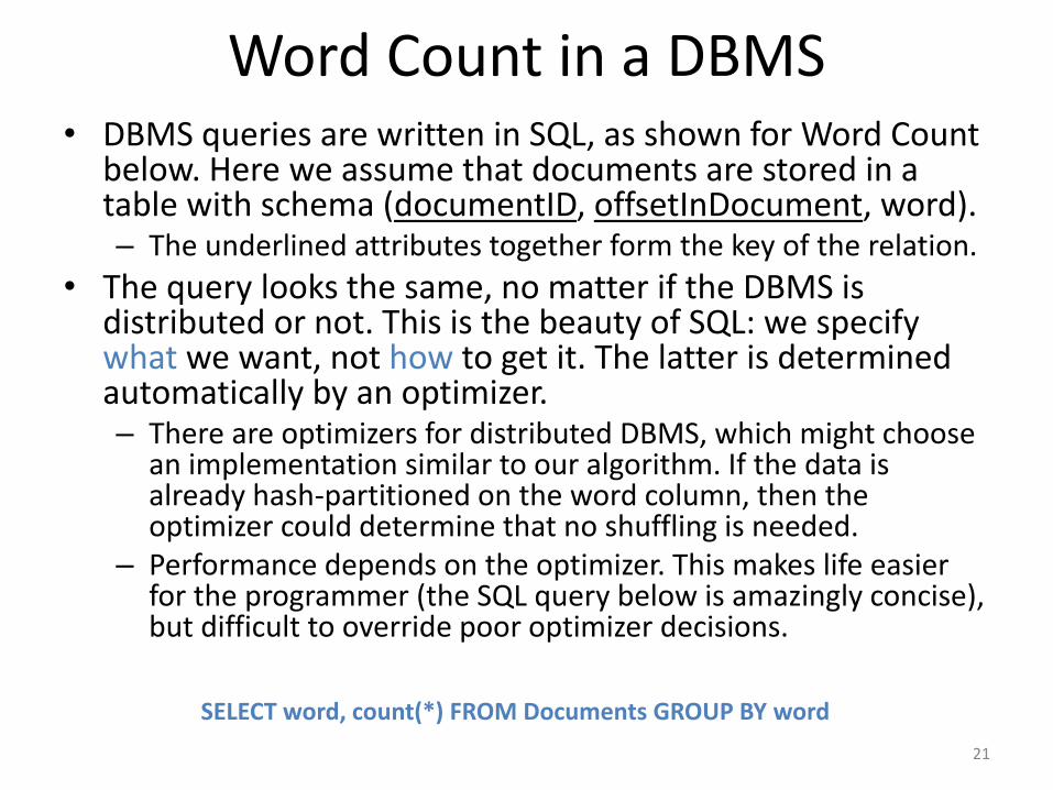
Word Count in a DBMS• DBMS queries are written in SQL, as shown for Word Count

below. Here we assume that documents are stored in a table with schema (documentID, offsetInDocument, word).– The underlined attributes together form the key of the relation.

• The query looks the same, no matter if the DBMS is distributed or not. This is the beauty of SQL: we specify what we want, not how to get it. The latter is determined automatically by an optimizer.– There are optimizers for distributed DBMS, which might choose

an implementation similar to our algorithm. If the data is already hash-partitioned on the word column, then the optimizer could determine that no shuffling is needed.

– Performance depends on the optimizer. This makes life easier for the programmer (the SQL query below is amazingly concise), but difficult to override poor optimizer decisions.

21

SELECT word, count(*) FROM Documents GROUP BY word

Word Count in MapReduce• The programmer specifies two functions: Map

and Reduce. They look like sequential functions, i.e., there is no multi-threading or parallelism in them. We simply define how to process a given input.– The program has a few more components, but we will

cover those later.

• Intuitively, Map sets up the shuffle phase, so that each Reduce call receives the right data for local computation.– It turns out that Map and Reduce can perfectly

implement local counting and final summation, respectively.

22

Word Count in MapReduce

23

b a c c

Map task 0 Map task 1 Map task 2

(a,1), (b, 1), (c, 2) (b, 3), (c, 1)(a,1), (b, 1), (c, 1), (d, 1)

Reduce task 0 Reduce task 1

Shuffle

(b, 5), (d, 1)(a,2), (c, 4)

a c d b b b c b

map( documentID d, word x )emit( x, 1 )

combine( word x, [n1, n2,…] )// Same as reduce below

reduce( word x, [n1, n2,…] )// Each n is a partial count for word x.total = 0for each n in input list

total += nemit( x, total )

Program Discussion• By default, for each file split, there is exactly one Map task

processing it. The Map task calls the Map function one-by-one on each record in the input file split. For word x, the Map call emits (x, 1) to signal that 1 more occurrence of x was found.– MapReduce works with key-value pairs. By convention, the first

component is the key; the second is the value.

• There is exactly one Reduce function call for every key, i.e., distinct word. It receives all local counts for that word and totals them.– Data is automatically moved by the MapReduce environment: it

groups all Mapper output by key and sends it to the corresponding Reduce task. The Reduce function call for a key receives all the values associated with that key, no matter which Map task emitted them on which worker.

• Note that in Map task 0, Map would emit (c, 1) twice instead of the desired (c, 2). Since Map here works on a single word at a time, it cannot produce the partial count. Fortunately, MapReduce supports a Combiner. It works like a Reducer but is executed in the Map task. Here it is identical to the Reducer.

24

Program Discussion (cont.)• The assignment of words to Reduce tasks is determined by

the Partitioner. The default hash Partitioner in MapReduce implements the desired assignment.

• The pseudocode is amazingly simple and concise. And it defines a parallel implementation that can employ hundreds or thousands of machines for huge document collections. The actual program, modulo boilerplate syntax in Java, is not much longer than the pseudocode!

• MapReduce does all the heavy lifting of grouping the intermediate results (i.e., those emitted by Map) by their key and delivering them to the right Reduce calls. Hence this program is even simpler than the corresponding sequential program that would need a HashMap data structure to count per word. Notice how MapReduce’s grouping by key eliminated the need for the HashMap!

25

Real Hadoop Code for Word Count

• We discuss the Word Count program that comes with the Hadoop 3.1.1 distribution.

• Large comment blocks were removed here for better readability. The full source code is available at http://khoury.northeastern.edu/home/mirek/code/WordCount.java

26

http://khoury.northeastern.edu/home/mirek/code/WordCount.java

27

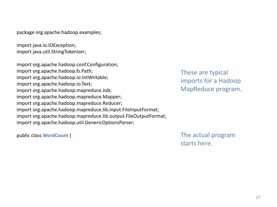
package org.apache.hadoop.examples;

import java.io.IOException;import java.util.StringTokenizer;

import org.apache.hadoop.conf.Configuration;import org.apache.hadoop.fs.Path;import org.apache.hadoop.io.IntWritable;import org.apache.hadoop.io.Text;import org.apache.hadoop.mapreduce.Job;import org.apache.hadoop.mapreduce.Mapper;import org.apache.hadoop.mapreduce.Reducer;import org.apache.hadoop.mapreduce.lib.input.FileInputFormat;import org.apache.hadoop.mapreduce.lib.output.FileOutputFormat;import org.apache.hadoop.util.GenericOptionsParser;

public class WordCount {

These are typical imports for a Hadoop MapReduce program.

The actual program starts here.

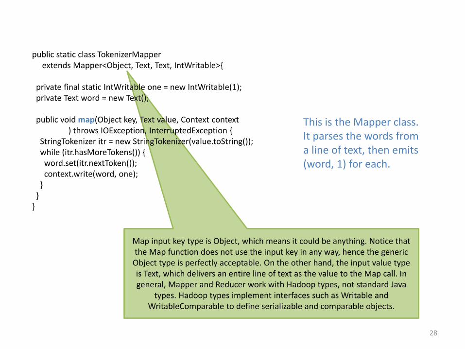
Map input key type is Object, which means it could be anything. Notice that the Map function does not use the input key in any way, hence the generic

Object type is perfectly acceptable. On the other hand, the input value type is Text, which delivers an entire line of text as the value to the Map call. In general, Mapper and Reducer work with Hadoop types, not standard Java

types. Hadoop types implement interfaces such as Writable and WritableComparable to define serializable and comparable objects.

28

public static class TokenizerMapperextends Mapper<Object, Text, Text, IntWritable>{

private final static IntWritable one = new IntWritable(1);private Text word = new Text();

public void map(Object key, Text value, Context context) throws IOException, InterruptedException {

StringTokenizer itr = new StringTokenizer(value.toString());while (itr.hasMoreTokens()) {word.set(itr.nextToken());context.write(word, one);

}}

}

This is the Mapper class. It parses the words from a line of text, then emits (word, 1) for each.

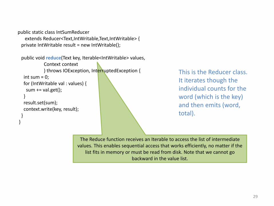
The Reduce function receives an Iterable to access the list of intermediate values. This enables sequential access that works efficiently, no matter if the

list fits in memory or must be read from disk. Note that we cannot go backward in the value list.

29

public static class IntSumReducerextends Reducer<Text,IntWritable,Text,IntWritable> {

private IntWritable result = new IntWritable();

public void reduce(Text key, Iterable<IntWritable> values, Context context) throws IOException, InterruptedException {

int sum = 0;for (IntWritable val : values) {sum += val.get();

}result.set(sum);context.write(key, result);

}}

This is the Reducer class. It iterates though the individual counts for the word (which is the key) and then emits (word, total).

Notice that the Combiner is set to the same class as the Reducer. This might not apply to other programs.

30

public static void main(String[] args) throws Exception {Configuration conf = new Configuration();String[] otherArgs = new GenericOptionsParser(conf, args).getRemainingArgs();if (otherArgs.length < 2) {System.err.println("Usage: wordcount <in> [<in>...] <out>");System.exit(2);

}Job job = Job.getInstance(conf, "word count");job.setJarByClass(WordCount.class);job.setMapperClass(TokenizerMapper.class);job.setCombinerClass(IntSumReducer.class);job.setReducerClass(IntSumReducer.class);job.setOutputKeyClass(Text.class);job.setOutputValueClass(IntWritable.class);for (int i = 0; i < otherArgs.length - 1; ++i) {FileInputFormat.addInputPath(job, new Path(otherArgs[i]));

}FileOutputFormat.setOutputPath(job,new Path(otherArgs[otherArgs.length - 1]));

System.exit(job.waitForCompletion(true) ? 0 : 1);}

}

The driver program puts everything together: It sets Mapper and Reducer class, and it controls the execution of the program.

Word Count in Spark• The Scala program below implements the same idea as the Hadoop

program:– The flatMap call splits a line of text into words.– The map call converts word x to (x, 1). Like MapReduce, the first component of

the pair is the key.– ReduceByKey automatically groups the (word, count) pairs by key and sums up

the counts.

• The program is very concise, but it does not reveal when data is shuffled. In a MapReduce program, we know that data is shuffled between Map and Reduce phase. For Spark we must know the semantics of operations like flatMap, map, and reduceByKey to know that only the latter requires shuffling.– It is also not obvious from the code if the equivalent of a Combiner is used.

31

val textFile = sc.textFile("hdfs://...")val counts = textFile.flatMap(line => line.split(" "))

.map(word => (word, 1))

.reduceByKey(_ + _)counts.saveAsTextFile("hdfs://...")

32

Let us now return to MapReduce and take a closer look at its features. Understanding MapReduce will help understanding the more complex Spark approach.

MapReduce Overview• MapReduce is a programming model and its implementation for

processing large data sets. The programmer essentially only specifies two (sequential) functions: Map and Reduce. At runtime, program execution is automatically parallelized.– MapReduce can be implemented on any architecture, but many design

decisions discussed in the Google paper, and implemented in Hadoop MapReduce, were influenced by the goal of running on a Warehouse-Scale Computer. Implementations for other architectures might affect design decisions to find the right balance between performance and fault tolerance.

• MapReduce provides a clever abstraction that works well for many real-world problems. It lets the programmer focus on the algorithm, while the system takes care of messy details such as:– Input partitioning and delivering data chunks to worker machines.– Creating and scheduling all tasks for execution on many machines.– Handling machine failures and slow responses.– Managing inter-machine communication to move intermediate results

from data producers to data consumers.

33

MapReduce Programming Model• A MapReduce program converts a list of key-value pairs to another list of key-value

pairs. Notice that the definitions below are more general than those in the Google paper. These general definitions correspond to Hadoop’s functionality.

• Map: (k1, v1) → list (k2, v2)– Map takes an input record, consisting of a key of type k1 and a value of type v1, and outputs a

list of intermediate key-value pairs, each of type k2 and v2, respectively. These types can be simple standard types such as integer or string, or complex user-defined ones.

– By design, Map calls are independent of each other. Hence Map can only perform per-record computations, but not combine information across different input records. For that, we need Combiners or similar task-level operations.

• MapReduce automatically groups all intermediate pairs with the same key together and passes them to Reduce.

• Reduce: (k2, list (v2)) → list (k3, v3)– Reduce combines information across records that share the same intermediate key. The

intermediate values are supplied via an iterator, which can read from a file.

• Terminology: There are 3 different types of keys: Map input keys k1, intermediate keys k2, and Reduce output keys k3. For MapReduce program design, only the intermediate keys matter, because they determine how records are assigned to Reduce calls. Following common practice, we will often simply say “key” instead of “intermediate key.”

34

MapReduce Execution Highlights• Each MapReduce job has its own application master, which schedules Map tasks

before Reduce tasks. It may schedule some Reduce tasks during the Map phase, so they can pull their data early from the Mappers.– The terms “Mapper” and “Reducer” are not used consistently. We use Mapper as a synonym

for Map task, which is an instance of the Mapper class; analogously for Reducer.

• When assigning Map tasks, the application master considers data location: It tries to assign a Map task to a machine that stores the corresponding input data chunk locally on disk. This avoids sending data across the network—an important optimization for big data. Since large files are already chunked up and distributed over many machines, this optimization is often very effective.– If no available machine has the chunk, then the master tries to assign the task to a machine in

the same rack as the data chunk. Moving data within a rack is faster (and only uses rack-local bandwidth) than sending it across the data center.

• A Mapper reads its file split from the distributed file system and emits its output to the local file system—partitioned by Reduce task and sorted by key within each of these partitions. The Mapper then informs the master about the file locations, who in turn informs the Reducers.

• Each Reducer pulls the corresponding data directly from the appropriate Mapper disk locations and merges the pre-sorted files locally by key before making them available to the Reduce function calls.

• The output emitted by Reduce is written to a local file. As soon as the Reduce task completes, this local file is atomically renamed (and moved) to a file in the DFS.

35

Summary of Important Hadoop Execution Properties

• Map calls inside a single Map task happen sequentially, consuming one input record at a time.

• Reduce calls inside a single Reduce task happen sequentially in increasing key order.

• There is no ordering guarantee between different Map tasks.

• There is no ordering guarantee between different Reduce tasks.

• Different tasks do not directly share any data with each other—not in memory and not on local disk.

36

Features Beyond Map and Reduce

• Even though the Map and Reduce functions usually represent the main functionality of a MapReduce program, there are several additional features that are crucial for achieving high performance and good scalability.

• We first take a closer look at the Combiner.

37

Combiner• Like a Reducer, the Combiner works on Map output by processing values

that share the same key. Often the code for a Combiner will be the same as the Reducer. Here are examples for when it is not:– Consider Word Count, but assume we are only interested in words that occur

at least 100 times in the document collection. The Reduce function computes the total count for a word, but outputs it only if it is at least 100. Should the Combiner do the same? No! The Combiner should not filter based on its local count. For instance, if there are 60 occurrences of “NEU” in one Mapper and 70 in another, then each is below 100, but the total exceeds the threshold and hence the count for “NEU” should be output.

– Consider computing the average of a set of numbers in Reduce. The Reduce function should output the average. The Combiner must output (sum, count) pairs to allow correct computation in the Reducer.

• Even though in Hadoop a Combiner is defined as a Reducer class, it is still executed in the Map phase. This has an interesting implication for its input and output types. Note that the Combiner’s input records are of type (k2, v2), i.e., Map’s output type. Since the Combiner’s output will be processed by a Reducer, and the Reducer input type is (k2, v2) as well, it follows that a Combiner’s input and output types must be identical.

38

Combiner (cont.)• Since the Combiner sees only a subset of the values for a key, the

Reducers still have work to do to combine the partial results produced by the Combiners. Such multi-step combining does not work for all problems. For example, it works for algebraic and distributive aggregate functions, but it cannot be applied to holistic aggregates.– For definitions of these classes of aggregates, see Jim Gray, Surajit Chaudhuri,

Adam Bosworth, Andrew Layman, Don Reichart, Murali Venkatrao, Frank Pellow, and Hamid Pirahesh. 1997. Data Cube: A Relational Aggregation Operator Generalizing Group-By, Cross-Tab, and Sub-Totals. Data Min. Knowl. Discov. 1, 1 (January 1997), 29-53. A summary is on the next slide.

• A Combiner represents an optimization opportunity. It can reduce data transfer cost from Mappers to Reducers (and the corresponding Reducer-side costs), but tends to increase Mapper-side costs for the additional processing.– Due to this tradeoff, Hadoop does not guarantee if or when a Combiner will be

executed. The programmer needs to ensure correctness, no matter how often and on what subset of the Map output records a Combiner might be executed. This includes ensuring correct behavior for cases where a Combiner execution works with both “raw” Map output and previously combined records.

39

Aggregates: Algebraic, Distributive, or Holistic?

• Consider a set of IJ values, which we assume to be arranged in a matrix { X(i,j) | i=1,…, I; j=1,…, J }. Intuitively, each row corresponds to a subset of the values we want to aggregate in the first round, while a second round combines the partial aggregates of the rows. Aggregate functions can be classified into 3 categories by their property of allowing such two-round aggregation:

• Aggregate function F() is distributive if there is a function G() such that F({ X(i,j) }) = G({ F({ X(i,j) | i=1,…, I}) | j=1,…, J }). COUNT(), MIN(), MAX(), SUM() are all distributive. In fact, F=G for all but COUNT(). G=SUM() for the COUNT() function.

• Aggregate function F() is algebraic if there is an M-tuple valued function G() and a function H() such that F({ X(i,j) }) = H({ G({ X(i,j) | i=1,…, I}) | j=1,…, J }). Average() and standard deviation are algebraic. For Average, function G() records the sum and count of the subset. The H() function adds component-wise and then divides to produce the global average. The key to algebraic functions is that a fixed size result (an M-tuple) can summarize the sub-aggregation.

• Aggregate function F() is holistic if there is no constant bound on the size of the storage needed to describe a sub-aggregate. That is, there is no constant M, such that an M-tuple characterizes the computation F({ X(i,j) | i=1,…, I}). Median(), MostFrequent() (also called the Mode()), and Rank() are common examples of holistic functions.

40

Partitioner• The Partitioner determines how intermediate keys are

assigned to Reduce tasks. Each Reduce task executes a Reduce function call for every key assigned to it.

• The MapReduce default Partitioner relies on a hash function to assign keys practically at random (but deterministically!) to Reduce tasks. This often balances load well, but there are many cases where clever design of the Partitioner can significantly improve performance or enable desired functionality. We will see examples in future modules.

• In Hadoop, we can create a custom Partitioner by implementing our own getPartition() method for the Partitioner class in org.apache.hadoop.mapreduce.

41

Maintaining Global State• Sometimes we would like to collect global statistics for a

MapReduce job, e.g., how many input records failed to parse in the Map phase. Unfortunately, tasks cannot directly communicate with each other and hence cannot agree on a global counter value.

• To get around this limitation, Hadoop supports global counters. These counters are modified by individual tasks, but all updates are propagated to the application master. The master therefore can maintain the value of each counter and make it available to the driver program.– The intended way of using counters is to (1) set an initial value in the

driver, then (2) increment or decrement the value in Mappers and Reducers, and (3) read the final value in the driver after the job completed.

• Since global counters are maintained centrally by the master and updates are sent from the different tasks, master and network can become a bottleneck if too many counters are managed. Hence it is not recommended to use more than a few hundred such counters.

42

Broadcasting Data to All Tasks• Hadoop supports two ways of sharing the same

data with all tasks.

• A small number of constants should be shared through the Context object, which is defined in the driver and passed to all tasks.

• For large data, use the file cache. By adding a file to the file cache, it will be copied to all worker machines executing MapReduce tasks.– No matter how many tasks a worker executes, it

receives only a single copy of the file and keeps it until the job completes. This avoids repeated copying of a file to the same worker.

43

Terminology Cheat Sheet• A MapReduce job consists of a Map phase and a Reduce phase,

connected through a shuffle phase.

• The Map phase executes several Map tasks. Each task executes the Map function exactly once for each input record in its input split.– Default number of Map tasks = number of input file splits– Number of Map function calls = number of input records

• The Reduce phase executes several Reduce tasks. Each task executes the Reduce function exactly once for each key in its input.– In Hadoop, Reduce function calls in a Reduce task happen in key order.– The number of Reduce tasks should be controlled by the programmer.– The assignment of keys to Reduce tasks is performed by the

Partitioner’s getPartition function. Given a key, it returns a Reduce task number.

44

Important Hadoop System Details

• The features discussed so far help the programmer implement their algorithm ideas. Below the surface, MapReduce does a lot of work that is hidden from the programmer, but still affects program performance. We will now take a closer look at some of these hidden features and processes.

45

Moving Data From Mappers to Reducers

• Data is transferred from Mappers to Reducers in the shuffle phase. It establishes a synchronization barrier between Map and Reduce phase, because no Reduce function call is executed until all Map output has been transferred. If a Reduce call were to be executed earlier, it might not have access to the complete list of input values.– During MapReduce job execution, reported Reduce progress may

exceed zero, while Map progress is still below 100%. How can this happen? Isn’t Reduce supposed to wait until all Mappers are done? Yes, it does! Here Hadoop already counts data transfer between Mappers and Reducers as Reduce progress.

• The shuffle phase can be the most expensive part of a MapReduce execution. It starts with Map function calls emitting data to an in-memory buffer. Once the buffer fills up, its content is partitioned by Reduce task (using the Partitioner) and the data for each task is sorted by key (using a key comparator than can be provided by the programmer). The partitioned and sorted buffer content is written to a spill file in the local file system. At some point spill files could be merged and the partitions copied to the corresponding Reducers.

46

Shuffle Phase Overview

47

Inputsplit

Map

Buffer in memory

Reduce

From other Maps

To other Reduce tasks

merge

Output

Map task Reduce taskSpill files on disk: partitioned by Reduce task, each partition sorted by key

Spilled to a new disk file when almost full

Spill files merged into a single output file

Fetch over HTTP

Reduce tasks can start copying data from a Map task as soon as it completes. Reduce cannot start processing the data until all Mappers have finished and all their output has arrived.

Merge happens in memory if data fits, otherwise also on disk

There are tuning parameters to control the performance of the shuffle phase.

Moving Data From Mappers to Reducers (Cont.)

• Each Reducer merges the pre-sorted partitions it receives from different Mappers. The sorted file on the Reducer is then made available for its Reduce calls. The iterator for accessing the Reduce function’s list of input values simply iterates over this sorted file.

• Notice that it is not necessary for the records assigned to the same partition to be sorted by key. It would be sufficient to simply group them by key. Grouping is slightly weaker than sorting, hence could be computationally less expensive.– In practice, grouping of big data is often implemented

through sorting anyway. Furthermore, the property that Reduce calls in the same task happen in key order can be exploited by MapReduce programs. We will see this in a future module for sorting and secondary sort.

48

Backup-Task Optimization• Toward the end of the Map phase, the application master might

create backup Map tasks to deal with machines that take unusually long for the last in-progress tasks (“stragglers”).– Recall that the Reducers cannot start their work until all Mappers have

finished. Hence even a single slow Map task would delay the start of the entire Reduce phase. Backup tasks, i.e., “copies” of a task that are started while the original instance of the task is still in progress, can address delays caused by slow machines.

• The same optimization can be applied toward the end of the Reduce phase to avoid delayed job completion due to stragglers.

• Will duplicate tasks jeopardize the correctness of the job result? No, they are handled by the MapReduce system. We will soon see how, when discussing failures.

• Side note: Sometimes the execution log of your MapReduce job will show error messages indicating task termination. Take a close look. Some of those may have been caused by backup task optimization when duplicate tasks were actively terminated by the application master.

49

Handling Failures• Since MapReduce was proposed for Warehouse-Scale

Computers, it must deal with failures as a common problem.

• MapReduce was designed to automatically handle system problems, making them transparent to the programmer.– The programmer does not need to write code for dealing with

slow responses or failures of machines in the cluster.

• When failures happen, typically the only observable effect is a moderate delay in program execution due to re-assignment of tasks from the failed machine.

• In Hadoop, hanging tasks are detected through timeout. The application master will automatically re-schedule failed tasks. It tries up to mapreduce.map.maxattempts many times (similar for Reduce).

50

Handling Worker Failures: Map• The master pings every worker machine periodically.

Workers who do not respond in time are marked as failed.

• A failed worker’s in-progress and completed Map tasks are reset to idle state and become available for re-assignment to another worker.– Why do we need to re-execute a completed Map task?

Mappers write their output to the local file system. When the machine that executed this Map task fails, the local file system is considered inaccessible and hence the result must be re-created on another machine.

• Reducers are notified by the master about the Mapper failure, so that they do not attempt to read from the failed machine.

51

Handling Worker Failures: Reduce

• A failed worker’s in-progress Reduce tasks are reset to idle state and become available for re-assignment to another worker machine. There is no need to restart completed Reduce tasks.

– Why not? Reducers write their output to the distributed file system. Hence even if the machine that produced the data fails, the file is still accessible.

52

Handling Master Failure• The application master rarely fails, because it is a single process. In

contrast, the probability of experiencing at least one failure among 100 or 1000 worker processes is much higher.

• The simplest way of handling a master failure is to abort the job. Users re-submit aborted jobs once the new master process is up. This works well if the master’s mean time to failure is significantly greater than the execution time of most MapReduce jobs.– To illustrate this, assume the master has a mean time to failure of 1

week. Jobs running for a few hours are unlikely to experience a master failure. However, a job running for 2 weeks has a high probability of suffering from a master failure. Abort-and-resubmit would not work well for such jobs, because the newly re-started instance of the job is likely to experience a master failure as well.

• As an alternative to abort-and-resubmit, the master could write periodic checkpoints of its data structures so that it can be re-started from a checkpointed state. Long-running jobs would pick up from this state, instead of starting from scratch. The downside of checkpointing is the higher cost during normal operation, compared to abort-and-resubmit.

53

Program Semantics with Failures• If Map, getPartition, and Combine functions are deterministic, then MapReduce

guarantees that the output of a computation, no matter the number of failures, is equivalent to a non-faulting sequential execution. This property relies on atomic commit of Map and Reduce outputs, which is achieved as follows:– An in-progress task writes its output to a private temp file in the local file system.– On completion, a Map task sends the name of its temp file to the master. The master ignores

this information if the task was already complete. (This could happen if multiple instances of a task were executed, e.g., due to failures or backup-task optimization.)

– On completion, a Reduce task atomically renames its temp file to a final output file in the distributed file system. This functionality needs to be supported by the distributed file system.

• For non-deterministic functions, it is theoretically possible to observe output that is not equivalent to a non-faulting sequential execution when (1) the re-execution of a task makes a different non-deterministic choice and (2) the output of both the original and the re-executed instance of the task are used in the computation. (This could be detected and fixed by MapReduce, at relatively high cost.)– Consider Map task m and Reduce tasks r1 and r2. Let e(r1) and e(r2) be the execution that

committed for r1 and r2, respectively. There can only be one committed execution for each Reduce task. Result e(r1) may have read the output produced by one execution of m, while e(r2) may have read the output produced by a different execution of m.

54

MapReduce in Action

• Let us discuss now how MapReduceperformed at Google.

• The results reported here are from Google’s original paper, published in 2004. While the specific numbers are outdated, the main message they convey has remained valid.

– And it is exciting to look at those original results ☺

55

MapReduce at Google• At the time, MapReduce was used at Google for implementing

parallel machine learning algorithms, clustering, data extraction for reports of popular queries, extraction of page properties, e.g., geographical location, and graph computations. Spark and high-level programming languages tailored to some of these applications have mostly replaced “raw” MapReduce.

• Google reported the following about their indexing system for Web search, which required processing more than 20 TB of data:– It consists of a sequence of 5 to 10 MapReduce jobs.– MapReduce resulted in smaller simpler code, requiring only about 700

LOC (lines of code) for one of the computation phases, compared to 3800 LOC before.

– MapReduce made it much easier to change the code. It is also easier to operate, because the MapReduce library takes care of failures.

– By design, MapReduce also made it easy to improve performance by adding more machines.

56

Experiments

• The experiments of the 2004 paper were performed on a cluster with 1800 machines. Each machine was equipped with a 2 GHz Xeon processor, 4 GB of memory, two 160 GB IDE disks. The machines were connected via a gigabit Ethernet link with less than 1 millisecond roundtrip time.

57

Grep

• The first experiment examines the performance of MapReduce for Grep. Grep scans 1010 100-byte records, searching for a rare 3-character pattern. This pattern occurs in 92,337 records, which are output by the program.

• The number of Map tasks is 15,000 (corresponding to the number of 64 MB splits); and there is only a single Reduce task.

• The graph above shows at which rate the Grep implementation in MapReduce consumes the input file as the computation progresses. Initially the rate increases as more Map tasks are assigned to worker machines. Then it drops as tasks finish, with the entire job being completed after about 80 sec.

• There is an additional startup overhead of about 1 minute beforehand, which is not shown in the graph. During this time, the program is propagated to the workers and the distributed file system is accessed for opening input files and getting information for locality optimization.

• Both the startup delay and the way how computation ramps up and then gradually winds down are typical for MapReduce program execution.

58

Sorting• The next experiment measures the time it takes to sort 1010

100-byte records, i.e., about 1 TB of data. The MapReduce program consists of less than 50 lines of user code. There are 15,000 Map tasks as for Grep, but the number of Reduce tasks is set to 4,000 to distribute the more substantial Reduce workload. For load balancing, key distribution information was used to enable intelligent partitioning. (We will discuss sorting in MapReduce in a future module.)

• Results:– The entire computation takes 891 sec.– It takes 1283 sec without the backup task optimization. This significant

slowdown by a factor of 1.4 is caused by a few slow machines.– Somewhat surprisingly, computation time increases only slightly to

933 sec if 200 out of 1746 worker machines are killed several minutes into the computation. This highlights MapReduce’s ability to gracefully handle even a comparably large number of failures.

59

60

We now discuss general principles for approaching a MapReduce programming problem, starting with the programming model’s expressiveness. In future modules we will see a variety of concrete examples.

Programming Model Expressiveness• The MapReduce programming model might appear limited, because it

relies on only a handful of functions and seems to have a comparably rigid structure for transferring data between worker nodes.

• However, it turns out that MapReduce is as powerful as the host language(e.g., Java) in which the programmer implements Map and Reduce functions. To see why, consider the following construction:– Consider a function F written in the host language that, given data set D,

outputs F(D). We show that we can write a MapReduce program that also returns F(D), no matter the input D.

– Map function: For input record r from D, emit (X, r).– Reduce function: Execute F on the list of input values.

• Since each record r is emitted with the same key X, the Reduce call for key X has access to the entire data set D. Hence it can execute F locally in the Reducer.

• Even though the above construction shows that every function F from the MapReduce host language can be computed in MapReduce, it would usually not result in an efficient or scalable parallel implementation. Our challenge therefore remains to find the best MapReduce implementation for a given problem.

61

Multiple MapReduce Steps• When multiple MapReduce jobs are needed to solve a more

complex problem, we can model such a MapReduce workflow as a directed acyclic graph. Its nodes are MapReduce jobs and an edge (J1, J2) indicates that job J2 is processing the output of job J1. A node may have multiple incoming and outgoing edges.

• We can execute such a workflow as a linear chain of jobs by executing the jobs in topological order. To run job J2 after job J1 in Hadoop, we need to create two Job objects and then include the following sequence in the driver program:– J1.waitForCompletion(); J2.waitForCompletion();

• Since job J1 might throw an exception, the programmer should include code that checks the return value and reacts to exceptions, e.g., by re-starting failed jobs in the pipeline.

• For more complex workflows, the linear chaining approach can become tedious. Then it is advisable to use frameworks with better workflow support, e.g., JobControl from org.apache.hadoop.mapreduce.lib.jobcontrol or Apache Oozie.

62

MapReduce Coding Summary1. Decompose a given problem into the

appropriate workflow of MapReduce jobs.2. For each job, implement the following:

1. Driver2. Mapper class with Map function3. Reducer class with Reduce function4. Combiner (optional)5. Partitioner (optional)

3. We might have to create custom data types as well, implementing the appropriate interfaces:1. WritableComparable for keys2. Writable for values

63

MapReduce Program Design Principles

• Focus on the question how to partition your input data and intermediate results.

• For tasks that can be performed independently on a data partition, use Map.

• For computation requiring data objects from different partitions, use Reduce.

• Sometimes it is easier to start program design with Map, sometimes Reduce. A good rule of thumb is to select intermediate keys and values such that the right objects end up together in the same Reduce function call.

64

High-Level MapReduce Development Steps

• Write Map and Reduce functions and create unit tests for them.• Write a driver program and run the job locally.

– Use a small data subset for testing and debugging on your development machine. Local testing can be performed using Hadoop’s local or pseudo-distributed mode.

• Once the local tests succeeded, run the program on the cluster using small input and few machines. Increase data size gradually to determine the relationship between input size and running time.

• Once you have an estimate of the running time on the full input, try it. Keep monitoring the cluster and cancel the job if it takes much longer than expected.

• Profile the code and fine-tune the program.– Analyze and think: where is the bottleneck and how do I address it?– Choose the appropriate number of Mappers and Reducers.– Consider Combiners. (We will discuss an alternative called in-Mapper

combining in a future module.)– Consider Map-output compression.– Explore Hadoop tuning parameters to optimize the shuffle phase between

Mappers and Reducers.

65

Local or Pseudo-Distributed Mode?• Hadoop’s local (also called standalone) mode runs the same

MapReduce user program as the distributed cluster version but executes it sequentially. It does not use any of the Hadoop daemons and it works directly with the local file system, hence does not require HDFS. This mode is perfect for development, testing, and initial debugging.– Since the program is executed sequentially, one can step through its

execution using a debugger, like for any sequential program.

• Hadoop’s pseudo-distributed mode also runs on a single machine but simulates a real Hadoop cluster by running all Hadoop daemons and using HDFS. This enables more advanced testing and debugging.– Consider a program using static members of Mapper or Reducer class

to share global state between all class instances. This does not work in a distributed system where the different class instances live in different JVMs. This bug would not surface in local mode.

• For most development, debugging, and testing, the local mode will be the better and easier choice.

66

Hadoop and Other Programming Languages

• The Hadoop Streaming API allows programmers to write Map and Reduce functions in languages other than Java. It supports any language that can read from standard input and write to standard output.

– Exchanging large objects through standard input and output may significantly slow down execution.

– The Hadoop Pipes API for C++ uses sockets for more efficient communication.

67

MapReduce Summary

• The MapReduce programming model hides details of parallelization, fault tolerance, locality optimization, and load balancing.

• The model is comparably simple, but it fits many common problems. The programmer provides a Map and a Reduce function, if needed also a Combiner and a Partitioner.

• The MapReduce implementation on a cluster scales to 1000s of machines.

68

69

Now we are ready to take a look at Spark as well.

Spark Overview• Spark builds on many of the same ideas as MapReduce, but

it hides data processing details even more from the programmer.– We will see the same functionality, including data partitioning,

combining, and shuffling.– Instead of just two functions (map, reduce), there are many

more. This reduces programming effort but makes it more challenging to select the right functions for a given problem.

• Spark increases the complexity of the program design space by letting programs manage data in memory across multiple rounds of local computation and data shuffling.– This creates opportunities for greater performance, but also for

making the wrong programming decisions.

• To better deal with Spark’s complexity, we will introduce its features and subtleties gradually over multiple modules.

70

Why Spark?• Spark introduced the notion of RDDs, a crucial abstraction

for distributed in-memory computation:– Ideally the input is loaded into memory once, then computation

happens in memory. This especially benefits iterative computations that repeatedly access the same data.

– This is not the same as using a shared-memory programming model: there is no notion of global data structures.

– In MapReduce, each job must load its input “from scratch.” Data cannot be kept in memory for later processing by another job.

• Lazy execution enables DBMS-style automatic optimization:– Spark can analyze and optimize an entire computation,

consisting of many non-trivial steps.– In MapReduce, a computation consists of independent jobs,

each consisting of a Map and a Reduce phase, which read from and write to slow storage, e.g., HDFS or S3. Optimization opportunities therefore are limited.

71

72

The following example illustrates thedifference between MapReduce andSpark for an iterative computation.

Compare data movement in each iteration, focusing on accesses to the DFS on the left. We discuss details when we introduce PageRank in a future lecture.

73

Typical iterative job (PageRank) in Hadoop MapReduce:

Typical iterative job (PageRank) in Spark:

GraphPR(nodeID, adjacency list,

PRvalue)

Worker(map)

Worker(reduce)Worker

(map)Worker(map)Worker

(map)

Worker(reduce)Worker

(reduce)Worker(reduce)

Graph

PR

Graph

Graph

new PR

PR up-dates

Graph(nodeID, adjacency list),

PR(nodeID, value)

Worker(map)Worker

(map)Worker(map)

Worker(Spark

executor)

Graph

PR

new PR

PR up-dates

Driver

new PR

One-time flow Per-iteration flow

Scala vs. Java

• Another argument you might hear: Spark programs are more elegant and concise, especially when written in Scala. MapReduce Java programs are more low-level, exposing messy implementation details.– One could write a compiler that converts a Spark

program to MapReduce. Similar things have been done before, e.g., for SQL (Hive) and PigLatin.

– However, since MapReduce lacks RDDs, the compiled program would still suffer from HDFS access cost, e.g., for iterative computations.

74

Spark Limitations• No in-place updates. MapReduce suffers from the same limitation,

but DBMS do support them.– Like MapReduce, Spark operations transform input to output. An

“update” would create a new copy of the modified dataset.– An OLTP workload in a DBMS consists of transactions that make

(small) changes to a (large) database. Creating an entire new copy of the database for an update is inefficient, therefore Spark does not support OLTP workloads well.

– Why this limitation? Without in-place updates, many problems of distributed data management go away (discussed in other modules).

• Optimized for batch processing. This also applies to MapReduce and DBMS, but the latter also excel at efficiently accessing small data fragments using indexes.– Like MapReduce, Spark shines when it comes to transforming a big

input “in bulk.” It therefore does not excel at real-time stream processing, where many small updates trigger incremental changes of a (large) system state.

– However, it can “simulate” stream processing by discretizing an input stream into a sequence of small batches.

75

Spark Components• The Spark system components mirror those of Hadoop MapReduce.• Client process: starts the driver, prepares the classpath and

configuration options for the Spark application, and passes application arguments to the application running in the driver.

• There is one driver per Spark application, which orchestrates and monitors the execution. It requests resources (CPU, memory) from the cluster manager, creates stages and tasks for the application, assigns tasks to executors, and collects the results.– Spark context and application scheduler are subcomponents of the

driver.

• Executor: a JVM process that executes tasks assigned to it by the driver. Executors have several task “slots” for parallel execution.– Each slot is executed as a separate thread. Their number could be set

greater than the number of physical cores available, in order to better use resources: while one thread is stalled waiting for data, another may take over a core.

76

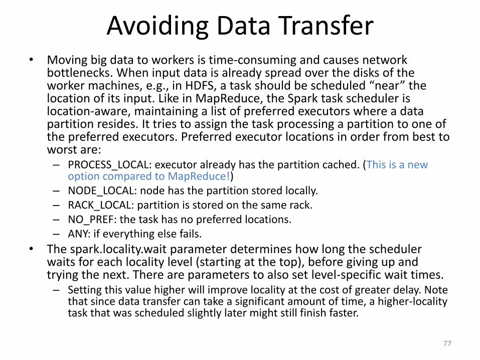
Avoiding Data Transfer• Moving big data to workers is time-consuming and causes network

bottlenecks. When input data is already spread over the disks of the worker machines, e.g., in HDFS, a task should be scheduled “near” the location of its input. Like in MapReduce, the Spark task scheduler is location-aware, maintaining a list of preferred executors where a data partition resides. It tries to assign the task processing a partition to one of the preferred executors. Preferred executor locations in order from best to worst are:– PROCESS_LOCAL: executor already has the partition cached. (This is a new

option compared to MapReduce!)– NODE_LOCAL: node has the partition stored locally.– RACK_LOCAL: partition is stored on the same rack.– NO_PREF: the task has no preferred locations.– ANY: if everything else fails.

• The spark.locality.wait parameter determines how long the scheduler waits for each locality level (starting at the top), before giving up and trying the next. There are parameters to also set level-specific wait times.– Setting this value higher will improve locality at the cost of greater delay. Note

that since data transfer can take a significant amount of time, a higher-locality task that was scheduled slightly later might still finish faster.

77

Spark Standalone Cluster• The Spark standalone cluster is appropriate when only Spark jobs execute on a

cluster. It uses Spark’s own scheduler to allocate resources.– For testing and debugging, use Spark local mode. A single JVM—the client JVM—executes

driver and a single executor. The executor can have multiple task slots, i.e., can execute tasks in parallel.

– For more advanced testing, local cluster mode runs a full Spark standalone cluster on the local machine. In contrast to full cluster mode, the master runs in the client JVM.

– For production, use the full cluster mode. Here the master process, which serves as the cluster resource manager, runs in its own JVM. To avoid slowing it down, it usually runs on a separate machine from the executors.

• The Spark scheduler has two policies for assigning executor slots to different Spark jobs: FIFO and FAIR. (Expect more to be added over time.)– With FIFO, resources are assigned in the order requested. Later jobs must wait in line. The

downside of this approach is that small jobs suffer from high latency when waiting for a big job to complete.

– FAIR addresses this issue by assigning executor slots to all active jobs round-robin. Hence a small job arriving late can still get resources quickly. However, big jobs take longer to finish. This can be fine-tuned through assignment to different scheduler pools.

• Spark also supports speculative execution (the same as backup-task optimization in MapReduce) to address the straggler problem: starting multiple instances of the same task as some tasks take too long or as the fraction of completed tasks reaches a certain threshold.

• There are two different modes, depending if the driver process is running in its own JVM on the cluster or in the client JVM: cluster- and client-deploy mode.

78

Cluster-Deploy Mode

79

Client JVM

Spark application

JVM heap

Scheduler

Spark context

Driver JVMJVM heap

T T

Executor JVM

JVM heap

T

Executor JVM

Cluster

Illustration based on Zecevic/Bonaci book

Interactions in Cluster-Deploy Mode

In a Spark standalone cluster, a “master” process acts as the cluster resource manager. Worker processes launch driver (in cluster-deploy mode only—in client-deploy mode it runs on the client!) and executors. If multiple applications are running concurrently on the same cluster, each has its own driver and executors.1. The client submits the application to the master.2. The master instructs a worker to launch the driver.3. The worker spawns a driver JVM.4. The master instructs the workers to launch executors

for the application.5. The workers spawn executor JVMs.6. Driver and executors communicate with each other

during execution.

80

Client-Deploy Mode

81

Spark application

JVM heap

Scheduler

Spark context

Client JVM

JVM heap

T T

Executor JVM

JVM heap

T

Executor JVM

Cluster

Driver


YARN Cluster• YARN is a popular cluster resource manager that was

originally introduced for Hadoop MapReduce. It supports different types of Java applications. On a YARN cluster, users may run Spark jobs as well as Hadoop jobs.

• YARN is a general resource manager as discussed earlier, i.e., it does not “understand” the anatomy or semantics of a Spark job. It simply communicates with the driver in terms of (1) receiving requests for resources and (2) making those resources available according to its scheduling policy.– The FIFO policy assigns resources as they become available to

the application who first requested them. Later requests must wait until earlier ones finish.

– The FAIR policy attempts to evenly balance resource assignment across requesters.

• Mesos is yet another option for cluster management, but we do not cover it.

82

83

Recall the discussion about YARN cluster interactions for resource requests.

Basic View of Cluster Resource Management

84

Client

Running on machine in-or outside the cluster

Cluster

Resource manager

1. Run this container. It needs 2 cores and 4 GB RAM.

2 cores4 GB Node

manager

Available: 1 core,16 GB

Node manager

Available: 8 cores,32 GB

Node manager


Node manager


Who Will Run the Application?

85

Client

Running on machine in-or outside the cluster

Cluster

Resource manager


2 cores4 GB Node

manager


Node manager


Node manager


Node manager


Too few cores.

Not enough memory

Possible

Possible

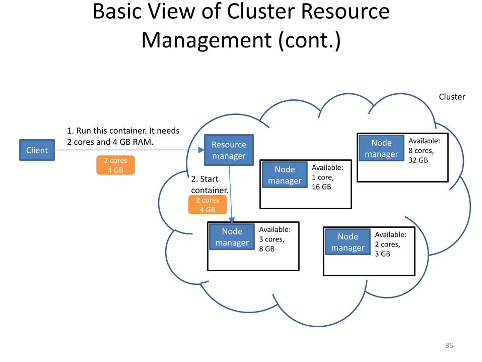
Basic View of Cluster Resource Management (cont.)

86

Client

Cluster

Resource manager


2 cores4 GB Node

manager


Node manager


Node manager


Node manager


2. Start container.

2 cores4 GB

Basic View of Cluster Resource Management (cont.)

87

Client

Cluster

Resource manager


2 cores4 GB Node

manager


Node manager


Node manager


Node manager


2. Start container.

2 cores4 GB

3. Application is running.

2 cores4 GB

3. Get status

88

Recall the discussion about starting up a Spark application in a YARN cluster.

89

Client JVM

Resource manager

Node manager

Node 1

Node 2

Node manager

YARN cluster (Spark in cluster deploy mode)


90

Client JVM

Resource manager

Node manager

Node 1

Node 2

Node manager

Get status



1: submit application

91

Client JVM

Resource manager

Node manager

Node 1

Node 2

Node manager

2: start application master (AM) container

Get status




92

Client JVM

Resource manager

Node manager

Scheduler

Spark context

Spark driver

Spark application master

JVM heap

Container

Node 1

Node 2

Node manager


3: launch AM container

Get status




93

Client JVM

Resource manager

Node manager

Scheduler

Spark context

Spark driver


JVM heap

Container

Node 1

Node 2

Node manager



4: request resources for application

Get status




94

Client JVM

Resource manager

Node manager

Scheduler

Spark context

Spark driver


JVM heap

Container

Node 1

Node 2

Node manager




5: start executor container


Get status




95

Client JVM

Resource manager

Node manager

Scheduler

Spark context

Spark driver


JVM heap

Container

Executor

JVM heap

Container

Node 1

Node 2

Node manager Executor

JVM heap

Container






6: launch executor container


Get status




96

Client JVM

Resource manager

Node manager

Scheduler

Spark context

Spark driver


JVM heap

Container

T

Executor

JVM heap

Container

Node 1

Node 2

Node manager

T

Executor

JVM heap

Container

T








7: Spark communication (independent of resource manager)

Get status




Programming in Scala

• We will use Scala to write Spark programs.

– It is the most elegant way of writing Spark programs.

– Some features are only available when using Scala.

– Spark is written in Scala.

– “Everybody” knows Java or Python, but Scala is a distinguishing skill.

– This course does not require advanced Scala skills,hence Scala should not become a heavy burden.

• However, if Scala represents too much of an obstacle for you, you can use Python or Java instead.

97

Compilation and Configuration Hints

• How do we include additional jar files in a Spark program? The recommended approach is to build an uberjar (aka fat jar).– Add each dependency to pom.xml.

– Use the maven-shade-plugin to have dependencies of dependencies recursively taken care off automatically.

• Spark configuration parameters can be set (1) on the commandline, (2) in Spark configuration files, (3) as system environment variables, and (4) by the user program. No matter what method you use, the parameters end up in the SparkConf object, which is accessible from SparkContext.– To view all parameters, use SparkContext’s getConf.getAll.

98

Addressing Memory Problems• Since Spark is optimized for in-memory execution, memory management

is crucial for performance.• The spark.executor.memory parameter determines the amount of

memory allocated for an executor. This is the amount the cluster manager allocates. The Spark tasks running in the executor must work with this amount.

• The executor uses spark.storage.memoryFraction (default 0.6) of it to cache data and spark.shuffle.memoryFraction (default 0.2) for temporary shuffle space.– spark.storage.safetyFraction (default 0.9) and spark.shuffle.safetyFraction

(default 0.8) provide extra headroom, because Spark cannot constantly detect exact memory usage. The actual part of the memory used for storage and shuffle is only 0.6*0.9 and 0.2*0.8, respectively.

• The rest of the memory is available for other Java objects and resources needed to run the tasks.

• Driver memory is controlled through spark.driver.memory (when starting the Spark application with spark-shell or spark-submit scripts) or the -XmxJava option (when starting from another application).

99

Spark Programming Overview

• Programming in Spark is like writing a “local” program in Scala for execution on a single machine.

• Parallelization, like in MapReduce, happens automatically under the hood.

• Pro: It is easy to write distributed programs.

– Compare Word Count in Spark with Hadoop.

• Con: It is also easy to write inefficientdistributed programs.

100

Refresher: Word Count in Spark

101

val textFile = sc.textFile("hdfs://...")

val counts = textFile.flatMap(line => line.split(" ")).map(word => (word, 1)).reduceByKey(_ + _)

counts.saveAsTextFile("hdfs://...")

Example from spark.apache.org/examples.html

Looking only at the code, can you tell when shuffling happens and if counts are aggregated within a task (like a Combiner) before shuffling?

Note: The reduce call could also be expressed equivalently as- reduceByKey((x,y) => (x+y)) or- reduceByKey(myFunction) // Assumes previous definition of myFunction(x:Int, y:Int) = x + y

Scala Function Literals• Functions play a crucial role in Scala. To understand what a program does,

we must understand the functions it uses. Let’s start with one of the simplest programs: return all lines in a text file that contain string “Spark.”

• The program first loads the input data:val myFile = sc.textFile( “/somePath/fileName” )– sc is the Spark Context and textFile loads the file into an RDD (a distributed

collection we will discuss soon) called myFile where each element is a line of text. Keyword val, in contrast to var, indicates that myFile is immutable.

– The path could refer to multiple files, e.g., using “*.txt”.

• The next line does all the work:val sparkLines = myFile.filter( line => line.contains(“Spark”) )– Filter returns all elements (i.e., lines of text) in myFile that satisfy the filter

condition, i.e., contain “Spark.”– The filter condition is also a function. It takes an element of myFile, named

line here, and returns true if that element contains “Spark” and false otherwise.• Function (x => y) converts x to y. In the example, x is a line of text and y is the output of

the contains() call on that line, checking if “Spark” is contained in the line.• It is an anonymous function, because it has no declared name. Hence it cannot be used

anywhere else. If we need the same function elsewhere, we need to define it again.• When do we use anonymous functions? When the function is not needed elsewhere, or

it is so simple that repeating it is preferable over separately defining and referencing it.

102

Alternative: Named Functions

103

Definition option 1:def hasSpark(line: String) = { line.contains(“Spark”) }

Definition option 2:val hasSpark = (line: String) => line.contains(“Spark”)

Usage:val sparkLines = myFile.filter(hasSpark)

Spark Data Representation• It helps to think of Spark’s abstractions for representing data as big

tables that are horizontally partitioned over multiple worker tasks.– A partition must fit into the worker task’s memory. If the cluster has

enough memory, all tasks of a Spark job may fit in memory at the same time, i.e., the entire table is spread over the combined cluster memory.

• Spark’s original data structure is the RDD. Intuitively, it is a table with a single column of type Object.

• The pair RDD is a table with two columns: key and value. It supports special _ByKey operations.

• A DataSet is a general table with any number of columns. It supports column operations such as grouping or sorting by one or more columns. DataFrame is a DataSet of tuples, which encodes relational tables for Spark SQL.

• We first illustrate the differences between the above data structures, then discuss them in more detail.

104

Spark Data Representation Example

105

Object of type String

(1, Amit, CS, 3.8)

(2, Bettina, CS, 4.0)

(3, Cong, ECE, 3.9)

Key of type String Value of type String

CS (1, Amit, 3.8)

ECE (2, Bettina, 4.0)

CS (3, Cong, 3.9)

ID: Int Name: String Department: String GPA: Float

1 Amit CS 3.8

2 Bettina ECE 4.0

3 Cong CS 3.9

RDD Pair RDD

DataSet, DataFrame

Discussion of the Example• RDDs feel familiar to many programmers: Each row contains some object or

record, making it easy to “dump” data into an RDD. However, when working with an RDD element, one must parse it on-the-fly to extract the relevant fields.

• For a pair RDD, the key must be chosen wisely so that the program can exploit the special _byKey operations.– Assume we want to analyze students by department. With department as the key, a simple

groupByKey() creates the desired value groups. With plain RDDs, each object must first be parsed using map() to extract the department field, before grouping can be applied.

• DataSet and DataFrame require the design of a table schema, but this investment will pay off in more elegant code and better performance.– Assume we want to compute the average GPA by department. The program can directly

specify a groupBy() on Department, followed by the aggregate on GPA. Realizing that the ID and Name columns are not referenced in the program, the Spark optimizer can automatically apply early projection, a classic database optimization technique that removes irrelevant table columns as early as possible, e.g., before shuffling.

– For both RDD and pair RDD, the GPA data is “hidden” inside a String object and hence needsto be extracted by the user program. Now the user is responsible for implementing early projection manually in user code.

• While it often is easier to find small code examples for (pair) RDDs, Spark is moving toward DataSets, because they offer greater flexibility and performance. An example is the Spark machine-learning library.

106

Shared Memory vs. Spark

107

B

C

A

B

A

C

Task 0

Task 1

Task 2

Shared memory: There are 3 different threads, concurrently trying to access the same shared data structure. This generally requires (1) the entire data structure to fit in memory and (2) careful use of locking or other concurrency-control mechanisms to prevent inconsistency. One can address (1) by

paging chunks of the data structure to secondary storage. Similarly, (2) could be addressed by careful ordering of operations, essentially simulating what happens in Spark.

Shared Memory vs. Spark

108

B

C

A

B

A

C

Task 0

Task 1

Task 2

Spark: Each task works on its own partition, processing it sequentially. No locking is necessary. Parallelism is achieved by scheduling multiple tasks concurrently. If there is enough memory for all 3

tasks, they can all be scheduled concurrently. Otherwise some tasks must wait until a previously scheduled task completes, freeing up a slot in the Spark Executor.

What is an RDD?

• Resilient Distributed Data Set = collection of elements that is– Immutable: one can read it, but not modify it.

(This avoids the hard problems in distributed data management.)

– Resilient: failures are transparent to the user, i.e., the user code does not need to handle those exceptions.

– Distributed: workers manages data partitions.

• The partitions field of an RDD is an Array, whose size corresponds to the number of partitions.

109

Working with RDDs

• Transformation = an operation that converts an RDD to another RDD. It does not trigger an actual execution (lazy evaluation).

• Action = an operation that triggers execution. It may return a result to the client program.

• From the name of the function, it is often not obvious which is which. Typically, actions return small (final) results.

110

Lazy Evaluation

• Transformations define a graph of operations—think “workflow”—the lineage of the RDD.

• Given the lineage and initial input, any partition of an RDD can be re-created.

– This is useful for fault tolerance or when RDD partitions are evicted from memory.

• An action triggers execution of all those transformations needed to produce the result of the action.

111

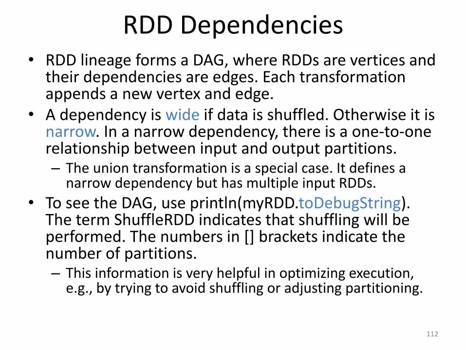
RDD Dependencies• RDD lineage forms a DAG, where RDDs are vertices and

their dependencies are edges. Each transformation appends a new vertex and edge.

• A dependency is wide if data is shuffled. Otherwise it is narrow. In a narrow dependency, there is a one-to-one relationship between input and output partitions.– The union transformation is a special case. It defines a

narrow dependency but has multiple input RDDs.

• To see the DAG, use println(myRDD.toDebugString). The term ShuffleRDD indicates that shuffling will be performed. The numbers in [] brackets indicate the number of partitions.– This information is very helpful in optimizing execution,

e.g., by trying to avoid shuffling or adjusting partitioning.

112

Program Execution

• A Spark job is divided into stages, defined by points where shuffles occur.

• For each stage, the driver creates tasks and sends them to the executors.

• The executors write their intermediate results to local disk. Shuffling is performed by special shuffle-map tasks.

• The last stage returns its results to the driver, using special results tasks.

113

114Example from on Zecevic/Bonaci book

val myList = List.fill(500) (scala.util.Random.nextInt(10) )val listRDD = sc.parallelize(myList, 5) // creates 5 partitions of the list

RDD lineage:

Driver

parallelize

listRDD

ParallelCollectionRDD

Stage 1


val myList = List.fill(500) (scala.util.Random.nextInt(10) )val listRDD = sc.parallelize(myList, 5) // creates 5 partitions of the listval pairs = listRDD.map(x => (x, x*x) )

RDD lineage:

Driver

parallelize map

listRDD pairs

ParallelCollectionRDD MapPartitionsRDD

OneToOnedependency

(narrow)

Stage 1


val myList = List.fill(500) (scala.util.Random.nextInt(10) )val listRDD = sc.parallelize(myList, 5) // creates 5 partitions of the listval pairs = listRDD.map(x => (x, x*x) )val reduced = pairs.reduceByKey( (v1, v2) => (v1+v2) )

RDD lineage:

Driver

parallelize map reduceByKey

listRDD pairs reduced

ParallelCollectionRDD MapPartitionsRDD ShuffledRDD

OneToOnedependency

(narrow)

Shuffledependency

(wide)

Stage 1 Stage 2


val myList = List.fill(500) (scala.util.Random.nextInt(10) )val listRDD = sc.parallelize(myList, 5) // creates 5 partitions of the listval pairs = listRDD.map(x => (x, x*x) )val reduced = pairs.reduceByKey( (v1, v2) => (v1+v2) )val finalRDD = reduced.mapPartitions( iter => iter.map({case(k, v) => “K=“+k+”, V=“+v}) ).collect()

RDD lineage:

Driver Driver

parallelize map reduceByKey map collect

listRDD pairs reduced finalRDD

ParallelCollectionRDD MapPartitionsRDD ShuffledRDD MapPartitionsRDD

OneToOnedependency

(narrow)

Shuffledependency

(wide)

OneToOnedependency

(narrow)

Stage 1 Stage 2

Pair RDD• Each element of a pair RDD is a key-value pair. This

corresponds to the way data is modeled in MapReduce. Often, a pair RDD is created by a function that emits output pairs, e.g., map(word => (word, 1)) in Word Count.

• Using a pair RDD, instead of a “plain” RDD, makes additional built-in functions available.– keys transformation returns the key “column” only. It is a

shortcut for map(_._1).– values transformation returns the value “column” only. It is

a shortcut for map(_._2).– countByKey() action returns a Scala Map containing each

key and its number of occurrences.– lookup(someKey) action returns the value for someKey.

118

More Pair RDD Functions• mapValues(oldVal => newVal) transformation

replaces for each key the old value with a new value. Here newVal stands not just for a constant but could be any kind of function applied to oldVal.

• flatMapValues(valueTransformationFunction) transformation associates each of the keys with zero or more new values. If the transformation function returns an empty list for a value, the corresponding element disappears. If the list has k>1 elements, the resulting pair RDD has k-1 additional elements.

119

More Pair RDD Functions• reduceByKey(mergeFunction) transformation

merges all values associated with the same key into a single value, using a merge function with signature (U, U) => U.– Input and output values of the merge function have

the same type. It merges two input values at a time, hence must be an associative function.

• foldByKey(zeroVal)(mergeFunction) transformation is the same as reduceByKey, but the additional parameter zeroVal allows more flexibility in defining the initial value.– The zeroVal is 0 for addition and counting, 1 for

multiplication, and Nil for lists.

120

foldByKey Example

121

RDD myNumberspartition 0: [(k1,2),(k5,4),(k1,6)]

myNumbers.foldByKey(0)((n1, n2) => n1+n2).collect()

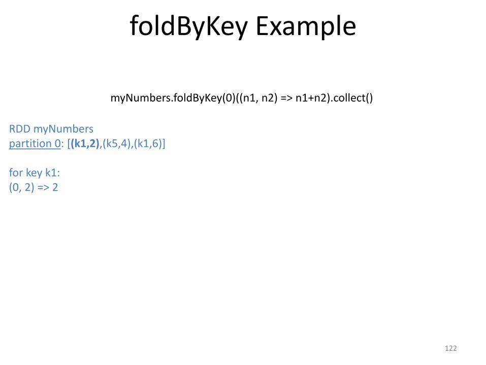
foldByKey Example

122


for key k1:(0, 2) => 2


foldByKey Example

123


for key k1:(0, 2) => 2

for key k5:(0, 4) => 4


foldByKey Example

124


for key k1:(0, 2) => 2

(2, 6) => 8

for key k5:(0, 4) => 4


foldByKey Example

125


for key k1:(0, 2) => 2

(2, 6) => 8

for key k5:(0, 4) => 4



for key k5:(0, 1) => 1

(1, 3) => 4

for key k1:(0, 5) => 5

foldByKey Example

126


for key k1:(0, 2) => 2

(2, 6) => 8

for key k5:(0, 4) => 4



for key k5:(0, 1) => 1

(1, 3) => 4

for key k1:(0, 5) => 5

Final aggregation:for key k1:(0, 8) => 8

(8, 5) => 13

for key k5:(0, 4) => 4

(4, 4) => 8

foldByKey Example

127


for key k1:(0, 2) => 2

(2, 6) => 8

for key k5:(0, 4) => 4



for key k5:(0, 1) => 1

(1, 3) => 4

for key k1:(0, 5) => 5

Final aggregation:for key k1:(0, 8) => 8

(8, 5) => 13

for key k5:(0, 4) => 4

(4, 4) => 8

What happens is we set zeroVal to 10, instead of 0?

aggregateByKey

• aggregateByKey(zeroVal)(transformFunction)(mergeFunction) transformation: The additional transformFunction with signature (U, V) => U “merges” values of type V into type U. Recall that mergeFunction has signature (U, U) => U, i.e., it can only aggregate type-U elements.– transformFunction is applied in each RDD partition to create

“local” aggregates. These are then merged, using mergeFunction.

128

aggregateByKey

• aggregateByKey(zeroVal)(transformFunction)(mergeFunction) transformation: The additional transformFunction with signature (U, V) => U “merges” values of type V into type U. Recall that mergeFunction has signature (U, U) => U, i.e., it can only aggregate type-U elements.– transformFunction is applied in each RDD partition to create

“local” aggregates. These are then merged, using mergeFunction.

129

What does this compute?

myNumbers.aggregateByKey((0, 0))(((s, c), v) => (s+v, c+1))(((s1,c1), (s2,c2)) => ((s1+s2), (c1+c2))).collect()

DataFrame and DataSet• Introduced in Spark 1.3, DataFrame is an RDD

with a schema. Like for a database table, the schema defines the name and type of each column.– The schema enables Spark to perform better

optimization of a computation.

• Introduced in Spark 1.6, DataSet generalizes DataFrame.

• They offer additional functionality compared to RDDs, similar to the key-based operations for pair RDDs.

• Internally, they are managed as RDDs. Hence all RDD functionality applies.

130

DataSet vs. Pair RDD• DataSet overall offers a better abstraction than

the limited pair RDD.– Consider a table with columns (year, month, day, sale).

To compute annual sales, a pair RDD needs to have year as the key. For an analysis of seasonal sales patterns, we need month as the key, or maybe a composite key (year, month). With pair RDDs, this requires clumsy data “re-formatting,” just to make the right column(s) become the key. With DataSets, all these different groupings can be performed on the same DataSet instance.

• Unfortunately, the semantics of DataSet functions can be a little more complex. This will be discussed in future modules.

131

Checkpointing

• Checkpointing persists an RDD and its lineage to disk. In contrast, RDD caching only manages the data, not the lineage.

• It is executed by the checkpoint operation, which must be called before any jobs are executed on the RDD.– Think of this as a materialized view.

• Checkpointing can be expensive, hence is typically used for large DAGs where re-creating partitions during failure would be too expensive.

132

Global State in Spark• Access to global state can simplify distributed-program design, but

maintaining global state requires communication—either among workers or with the application master.– Formally, global state requires consensus between participants. This is a well-

known challenging problem in distributed systems. Think about machines not responding, delayed responses, messages being lost or corrupted, and how to determine if a machine has really failed. (To learn more, check out concepts such as fail-stop and Byzantine failure.)

• To avoid high communication cost and delay, global state should be kept to a minimum:– Use it for variables that generate low update traffic. For instance, sum and

count aggregates can be accumulated locally, sending intermediate aggregates periodically to the master.

– Use it for critical program analysis, e.g., the amount of data generated globally or to count number of parsing errors across partitions.

– Use it for variables that would be difficult to compute otherwise, e.g., total PageRank mass in dangling nodes. (Discussed in a later module.)

– Do not use it for large objects that require frequent updates.

• To prevent programmers from writing inefficient code, Spark offers limited functionality for global variables: accumulators and broadcast variables.

133

Accumulators• Like global counters in MapReduce, accumulators implement global sums and

counts, allowing only adding of values. The older Accumulator and Accumulableclasses are deprecated as of Spark 2.0. Use AccumulatorV2 instead, which allows input and output type to differ.– Define custom accumulators by extending AccumulatorV2[IN, OUT], implementing functions

add, merge, copy, reset, isZero, and value.– It might be fun to subvert the accumulator by encoding complex objects in it. This may result

in poor performance and does not substitute for good distributed-algorithm design!

• How they should be used:– Create accumulator with Spark context in the driver; set initial value in the driver.– Update it in the executors.– Read its value in the driver. The value cannot be read by the executors, i.e., in a task.

134

// abstract class AccumulatorV2[IN, OUT] extends Serializable// class LongAccumulator extends AccumulatorV2[Long, Long]// spark refers to a SparkSession object.val lineCount = spark.sparkContext.longAccumulator

myRDD.foreach(line => lineCount.add(1)) // This operation is applied to an RDD partition, i.e., in a taskprintln(lineCount.value) // For println, the argument is sent to the driver. Hence this operation happens in the driver.

// This throws an exceptionmyRDD.foreach(line => lineCount.value) // This operation is applied to an RDD partition, i.e., in a task

Broadcast Variables• Broadcast variables can hold any serializable object. In contrast to accumulators,

they cannot be modified by executors. They are created in the driver, then sent to all executors.

• A broadcast variable’s value is sent at most once to each machine, where it is stored in memory.– When an executor tries to read the variable, it first checks if it has been loaded already. If not,

it requests it from the driver, one chunk at a time. By using this on-demand pull-based approach, a data transfer peak at job startup time is avoided.

– The broadcast uses a peer-to-peer gossip protocol like BitTorrent, i.e., the workers communicate directly with each other. This avoids a bottleneck at the master.

– Using destroy, a broadcast variable can be removed from executors and driver. Unpersist only removes it from executor cache. With these commands, resources, in particular memory, can be freed up earlier. (By default, Spark will unpersist the variable when it goes out of scope.)

• Spark configuration parameters specify the chunk size for transferring the broadcast variable and whether the data will be compressed for transfer.

135

// Broadcast data set myDataval bcastSet = sc.broadcast(myData)

// Accessing the broadcast data… bcastSet.value.someFunction(…)

Need for Broadcast Variables• Variables created in the driver and used by tasks are

automatically serialized and shipped with the tasks. Then why do we need special broadcast variables?

• Consider multiple tasks of a job assigned to the same executor. The above mechanism sends multiple copies of the same variable to the executor—one for each task that needs it. With a broadcast variable, there is only one copy per executor.– This is like MapReduce’s file cache.

• Of course, this is only worth the programming effort if the variable to be broadcast is fairly large.

• And it only reduces data traffic, if sufficiently many tasks need it: The default mechanism of shipping data to tasks only sends the data needed by the task!

136

Controlling RDD Partitions• The Partitioner object performs RDD partitioning. The

default is HashPartitioner. It assigns an element e to partition hash(e) % numberOfPartitions.– hash(e) is the key’s hash code for pair RDDs, otherwise the

Java hash code of the entire element.

– The default number of partitions is determined by Spark configuration parameter spark.default.parallelism.

• Alternatively, one can use RangePartitioner. It determines range boundaries by sampling from the RDD. (It should ideally use quantiles.)

• For pair RDDs, one can define a custom Partitioner.

137

Data Shuffling• Some transformations preserve partitioning, e.g.,

mapValues and flatMapValues.• Changes to the Partitioner, including changing the number

of partitions, requires shuffling.• map and flatMap remove the RDD’s Partitioner, but do not

result in shuffling. But any transformation that adds a Partitioner, e.g., reduceByKey, results in shuffling. Transformations causing a shuffle after map and flatMap:– Pair RDD transformations that change the RDD’s Partitioner:

aggregateByKey, foldByKey, reduceByKey, groupByKey, join, leftOuterJoin, rightOuterJoin, fullOuterJoin, subtractByKey

– RDD transformations: subtract, intersection, groupWith.– sortByKey (always causes shuffle)– partitionBy and coalesce with shuffle=true setting.

138

Challenge Question• Why does mapValues preserve the pair RDD’s

Partitioner, while map removes it?– In a pair RDD, the Partitioner depends only on the key.

– Function mapValues cannot modify the key, therefore the partitions of the resulting pair RDD are guaranteed to be consistent with the old Partitioner.

– Function map may modify the key. This means that the partitions of the resulting pair RDD may not be consistent with the old Partitioner.• To guarantee consistency, the new pair RDD would need to

be reshuffled, which is undesirable from a performance point of view and counterintuitive, because the programmer expects map to not shuffle data.

139

Challenge Question• Why does mapValues preserve the pair RDD’s

Partitioner, while map removes it?– In a pair RDD, the Partitioner depends only on the key.

– Function mapValues cannot modify the key, therefore the partitions of the resulting pair RDD are guaranteed to be consistent with the old Partitioner.

– Function map may modify the key. This means that the partitions of the resulting pair RDD may not be consistent with the old Partitioner.• To guarantee consistency, the new pair RDD would need to

be reshuffled, which is undesirable from a performance point of view and counterintuitive, because the programmer expects map to not shuffle data.

140

Changing Partitioning at Runtime• partitionBy(partitionerObject) transformation for pair

RDDs: If and only if the new Partitioner is different from the current one, a new RDD is created and data is shuffled.

• coalesce(numPartitions, shuffle?) transformation splits or unions existing partitions—depending if numPartitions is greater than the current number of partitions. It tries to balance partitions across machines, but also to keep data transfer between machines low.– repartiton is coalesce with shuffle? = true.

• repartitionAndSortWithinPartitions(partitionerObject) transformation for pair RDDs with sortable keys always shuffles the data and sorts each partition. By folding the sorting into the shuffle process, it is more efficient then applying partitioning and sorting separately.– Check: When would this be used in practice?

141

Mapping at Partition Granularity• mapPartitions(mapFunction) transformation: mapFunction has signature

Iterator[T] => Iterator[U]. Contrast this to map, where mapFunction has signature T => U.

• Why is this useful? Assume, like in Mapper or Reducer class in MapReduce, you want to perform setup and cleanup operations before and after, respectively, processing the elements in the partition. Typical use cases are (1) setting up a connection, e.g., to a database server and (2) creating objects, e.g., parsers that are not serializable, that are too expensive to be created for each element. You can do this by writing a mapFunction like this:– Perform setup operations, e.g., instantiate parser.– Iterate through the elements in the partition, e.g., apply parser to element.– Clean up.

• mapPartitionsWithIndex(idx, mapFunction) transformation also accepts a partition index idx, which can be used in mapFunction.

• Both operations also have an optional parameter preservePartitioning, by default set to false. Setting false results in removal of the partitioner.

142

Shuffle Implementation

• Shuffling is implemented by sorting or hashing.

• Parameter spark.shuffle.manager specifies which is used. Sort is the default, because it uses less memory and creates fewer files. However, sorting has higher computational complexity than hashing.

• Several other parameters control options such as consolidation of intermediate files, shuffle memory size, and if spilled data are compressed.

143

References• Jeffrey Dean and Sanjay Ghemawat. MapReduce: Simplified Data

Processing on Large Clusters. OSDI'04: Sixth Symposium on Operating System Design and Implementation, San Francisco, CA, December, 2004– https://scholar.google.com/scholar?cluster=10940266603640308767&

hl=en&as_sdt=0,22

• Matei Zaharia, Mosharaf Chowdhury, Michael J. Franklin, Scott Shenker, and Ion Stoica. 2010. Spark: cluster computing with working sets. In Proc. of the 2nd USENIX conference on Hot topics in cloud computing (HotCloud’10)– https://scholar.google.com/scholar?cluster=14934743972440878947&

hl=en&as_sdt=0,22

• Rundong Li, Ningfang Mi, Mirek Riedewald, Yizhou Sun, and Yi Yao. Abstract Cost Models for Distributed Data-Intensive Computations. In Distributed and Parallel Databases 37(3): 411-439 (2019), Springer– http://www.ccs.neu.edu/home/mirek/papers/2018-DAPD-

AbstractCostModels-preprint.pdf

144

https://scholar.google.com/scholar?cluster=10940266603640308767&hl=en&as_sdt=0,22


http://www.ccs.neu.edu/home/mirek/papers/2018-DAPD-AbstractCostModels-preprint.pdf

References

• Jim Gray, Surajit Chaudhuri, Adam Bosworth, Andrew Layman, Don Reichart, Murali Venkatrao, Frank Pellow, and Hamid Pirahesh. 1997. Data Cube: A Relational Aggregation Operator Generalizing Group-By, Cross-Tab, and Sub-Totals. Data Min. Knowl. Discov. 1, 1 (January 1997), 29-53

– https://scholar.google.com/scholar?cluster=10836794633940449959&hl=en&as_sdt=0,22

145
