overview of adiabatic quantum computationamchilds/talks/cifar13-tutorial.pdf · overview of...
TRANSCRIPT
Overview of adiabatic quantum computation
Andrew Childs
Adiabatic optimization
Quantum adiabatic optimization is a class of procedures for solving optimization problems using a quantum computer. !Basic strategy: • Design a Hamiltonian whose ground state encodes the
solution of an optimization problem. • Prepare the known ground state of a simple Hamiltonian. • Interpolate slowly. !Proposed in the context of quantum computation by Farhi, Goldstone, Gutmann, and Sipser (2000). Related ideas suggested by Kadowaki and Nishimori (1998), Brooke, Bitko, Rosenbaum, and Aeppli (1999), and others.
Outline• Quantum computation and Hamiltonian dynamics • Simulated vs. actual dynamics • The adiabatic theorem • Adiabatic optimization and spectral gaps • Examples • Robustness of adiabatic quantum computation • Universal quantum computation • Open problems
- Stoquastic Hamiltonains - Fault tolerance
Hamiltonian dynamics
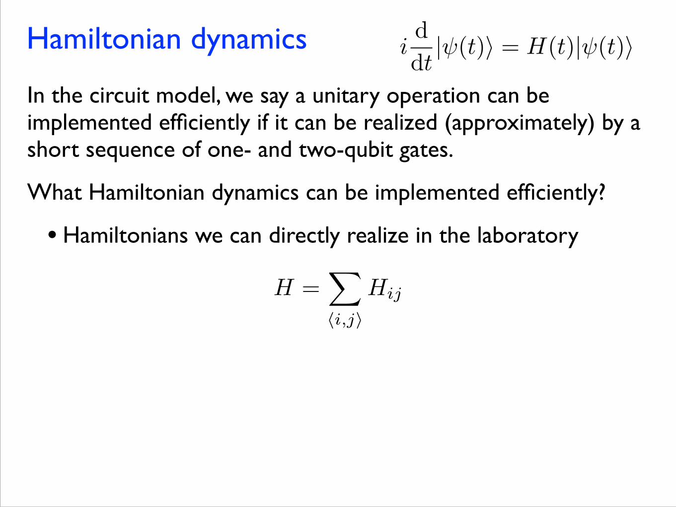
In the circuit model, we say a unitary operation can be implemented efficiently if it can be realized (approximately) by a short sequence of one- and two-qubit gates.
What Hamiltonian dynamics can be implemented efficiently?
iddt
| (t)i = H(t)| (t)i
Hamiltonian dynamics
In the circuit model, we say a unitary operation can be implemented efficiently if it can be realized (approximately) by a short sequence of one- and two-qubit gates.
What Hamiltonian dynamics can be implemented efficiently?
• Hamiltonians we can directly realize in the laboratory
H =X
hi,ji
Hij
iddt
| (t)i = H(t)| (t)i

Hamiltonian dynamics
In the circuit model, we say a unitary operation can be implemented efficiently if it can be realized (approximately) by a short sequence of one- and two-qubit gates.
What Hamiltonian dynamics can be implemented efficiently?
• Hamiltonians we can directly realize in the laboratory
!
!
• Hamiltonians we can efficiently simulate using quantum circuits (all of the above, plus sparse Hamiltonians, etc.)
H =X
hi,ji
Hij
iddt
| (t)i = H(t)| (t)i
Simulated vs. actual dynamics
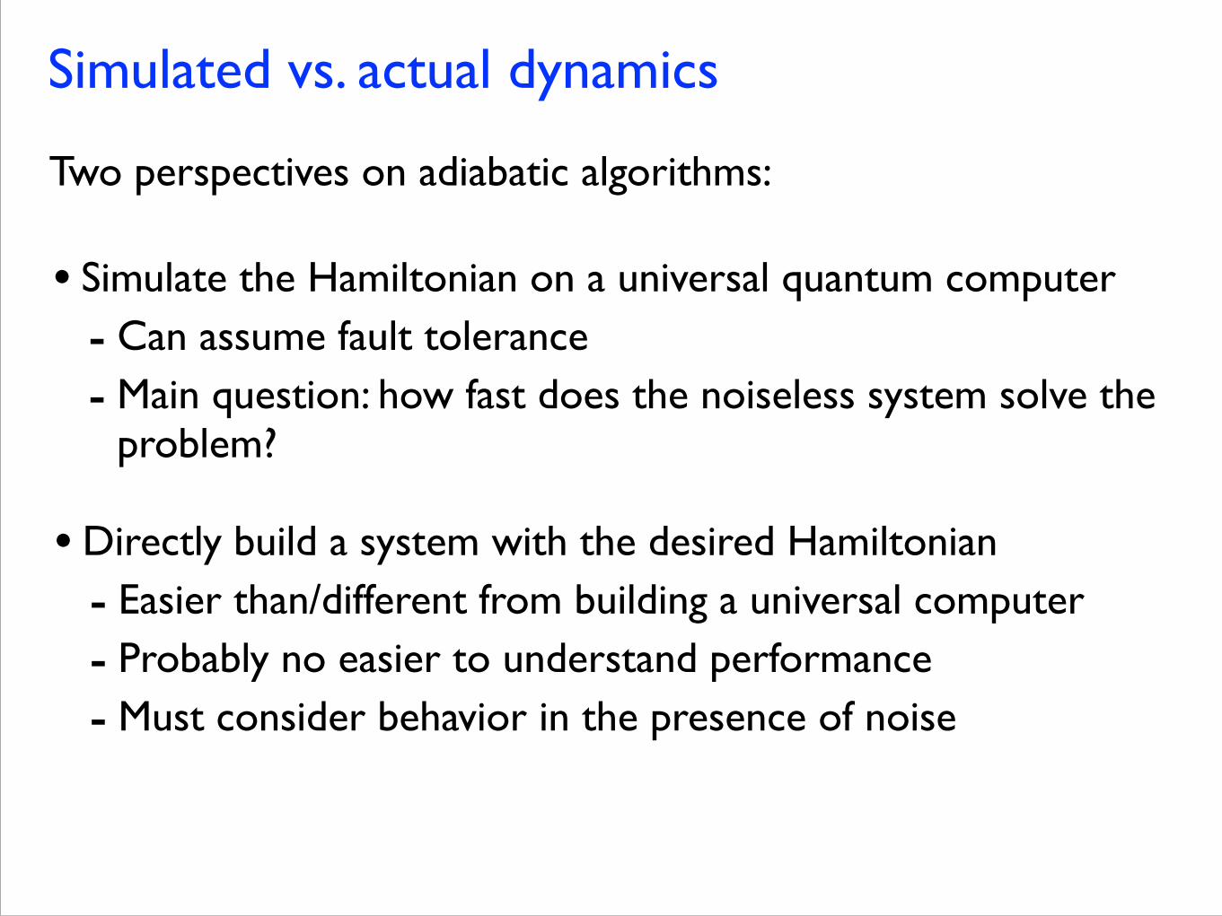
Two perspectives on adiabatic algorithms:
• Directly build a system with the desired Hamiltonian - Easier than/different from building a universal computer - Probably no easier to understand performance - Must consider behavior in the presence of noise
• Simulate the Hamiltonian on a universal quantum computer - Can assume fault tolerance - Main question: how fast does the noiseless system solve the
problem?
The adiabatic theorem
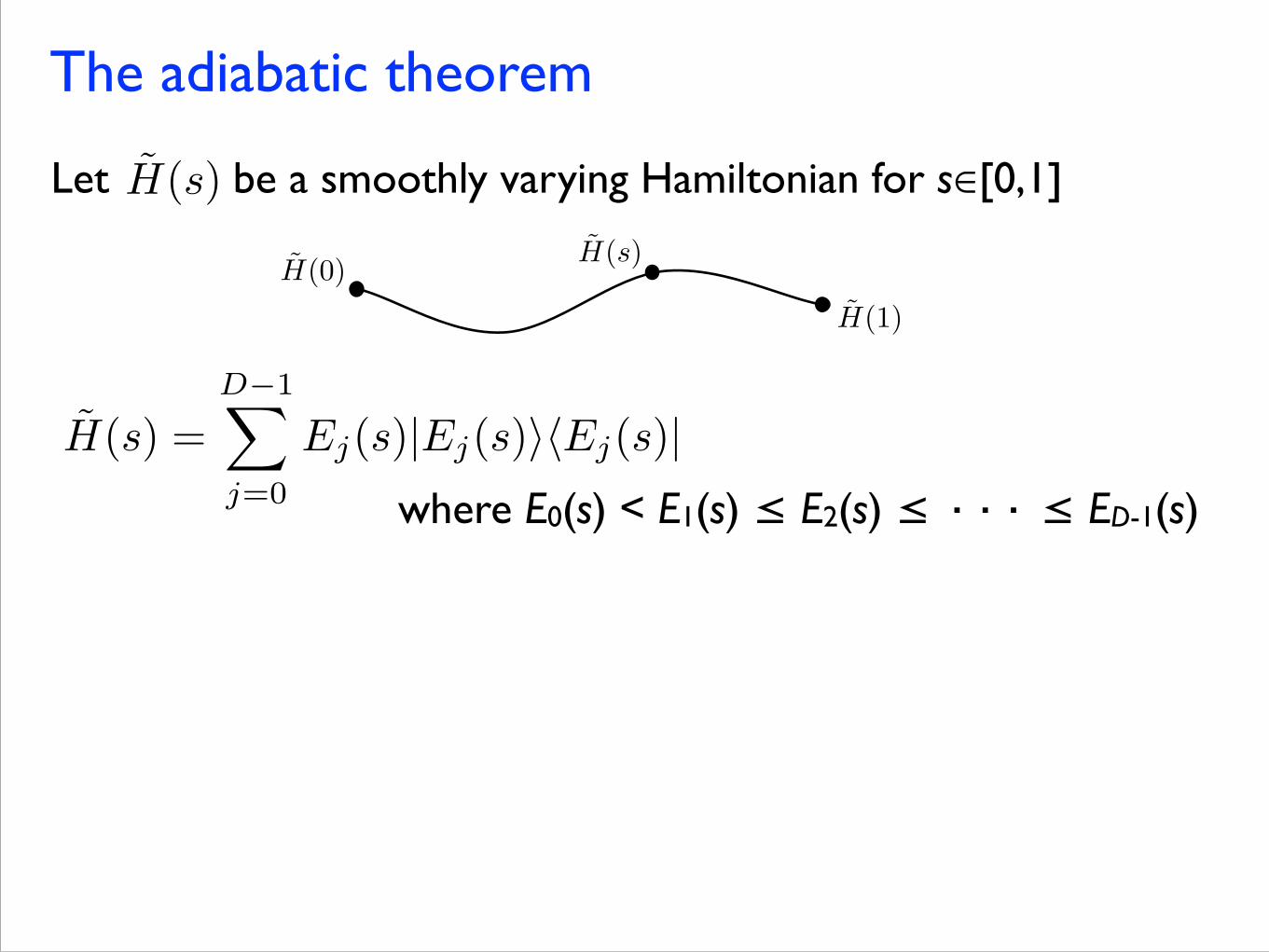
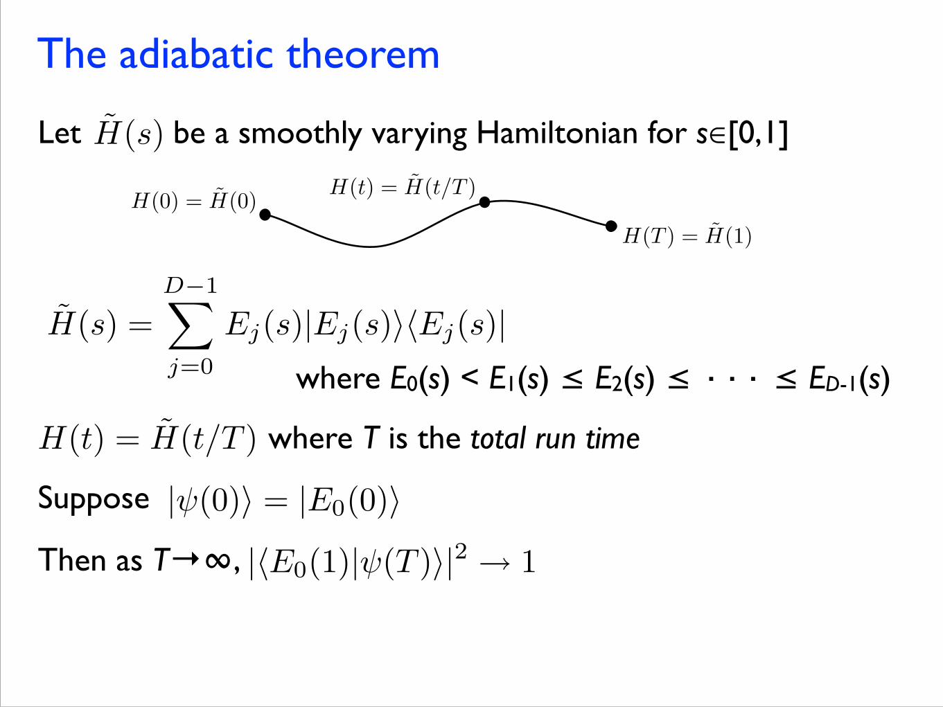
Let be a smoothly varying Hamiltonian for s∈[0,1]
!
!
!
where E0(s) < E1(s) ≤ E2(s) ≤ ··· ≤ ED-1(s)
H̃(s)
H̃(s) =D�1X
j=0
Ej(s)|Ej(s)ihEj(s)|
H̃(0)H̃(1)
H̃(s)
The adiabatic theorem
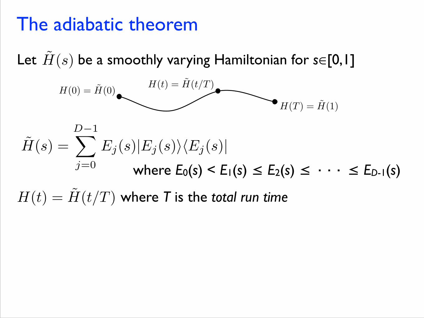
Let be a smoothly varying Hamiltonian for s∈[0,1]
!
!
!
where E0(s) < E1(s) ≤ E2(s) ≤ ··· ≤ ED-1(s)
where T is the total run time
H̃(s)
H̃(s) =D�1X
j=0
Ej(s)|Ej(s)ihEj(s)|
H(0) = H̃(0) H(t) = H̃(t/T )
H(T ) = H̃(1)
H(t) = H̃(t/T )
The adiabatic theorem
Let be a smoothly varying Hamiltonian for s∈[0,1]
!
!
!
where E0(s) < E1(s) ≤ E2(s) ≤ ··· ≤ ED-1(s)
where T is the total run time
Suppose
Then as T→∞,
H̃(s)
H̃(s) =D�1X
j=0
Ej(s)|Ej(s)ihEj(s)|
|hE0(1)| (T )i|2 ! 1
| (0)i = |E0(0)i
H(0) = H̃(0) H(t) = H̃(t/T )
H(T ) = H̃(1)
H(t) = H̃(t/T )

The adiabatic theorem
Let be a smoothly varying Hamiltonian for s∈[0,1]
!
!
!
where E0(s) < E1(s) ≤ E2(s) ≤ ··· ≤ ED-1(s)
where T is the total run time
Suppose
Then as T→∞,
For large T, . But how large must it be?
H̃(s)
H̃(s) =D�1X
j=0
Ej(s)|Ej(s)ihEj(s)|
|hE0(1)| (T )i|2 ! 1
| (0)i = |E0(0)i
| (T )i ⇡ |E0(1)i
H(0) = H̃(0) H(t) = H̃(t/T )
H(T ) = H̃(1)
H(t) = H̃(t/T )
Approximately adiabatic evolution
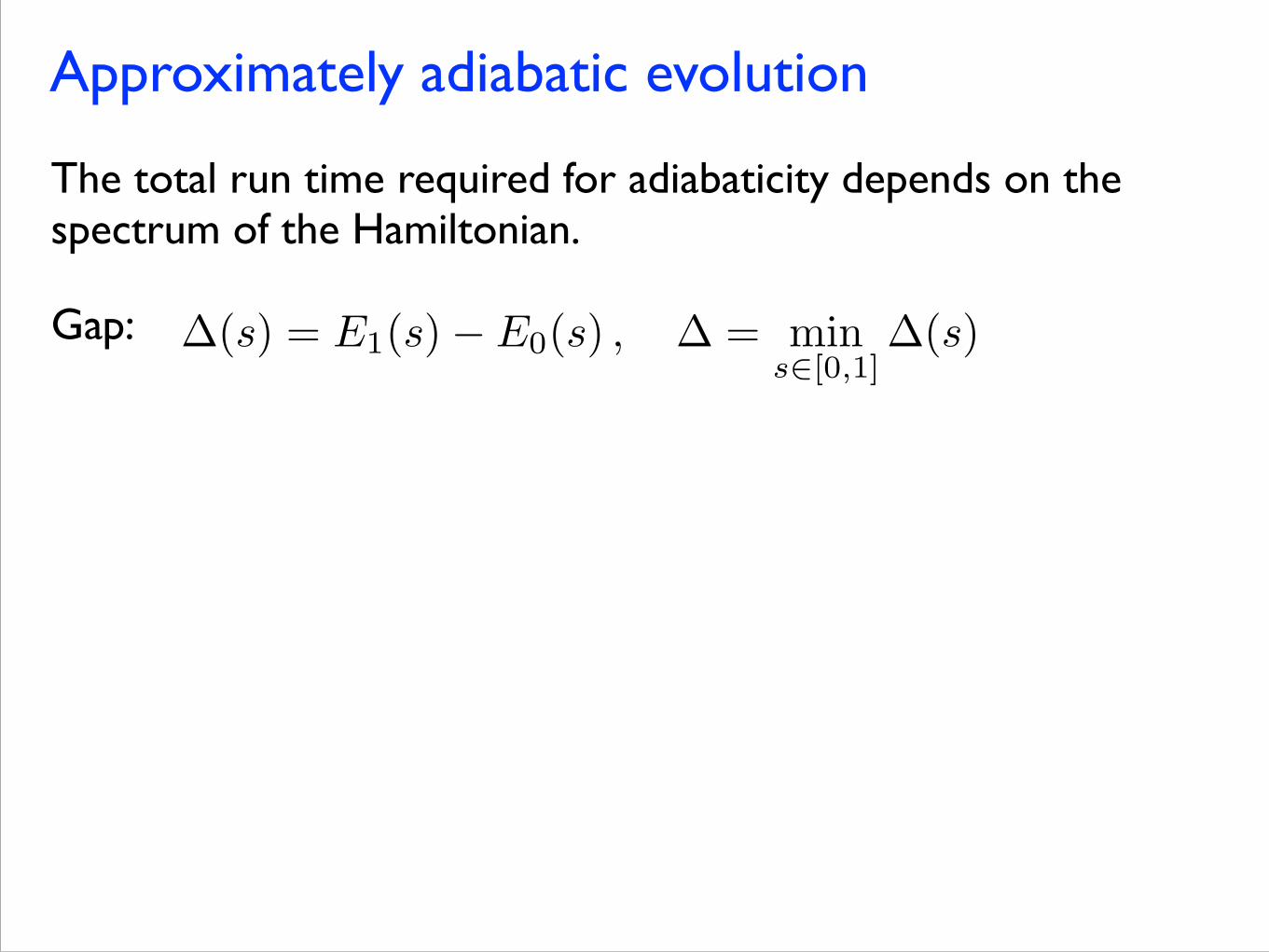
The total run time required for adiabaticity depends on the spectrum of the Hamiltonian.
Gap: �(s) = E1(s)� E0(s) , � = mins2[0,1]
�(s)
Approximately adiabatic evolution
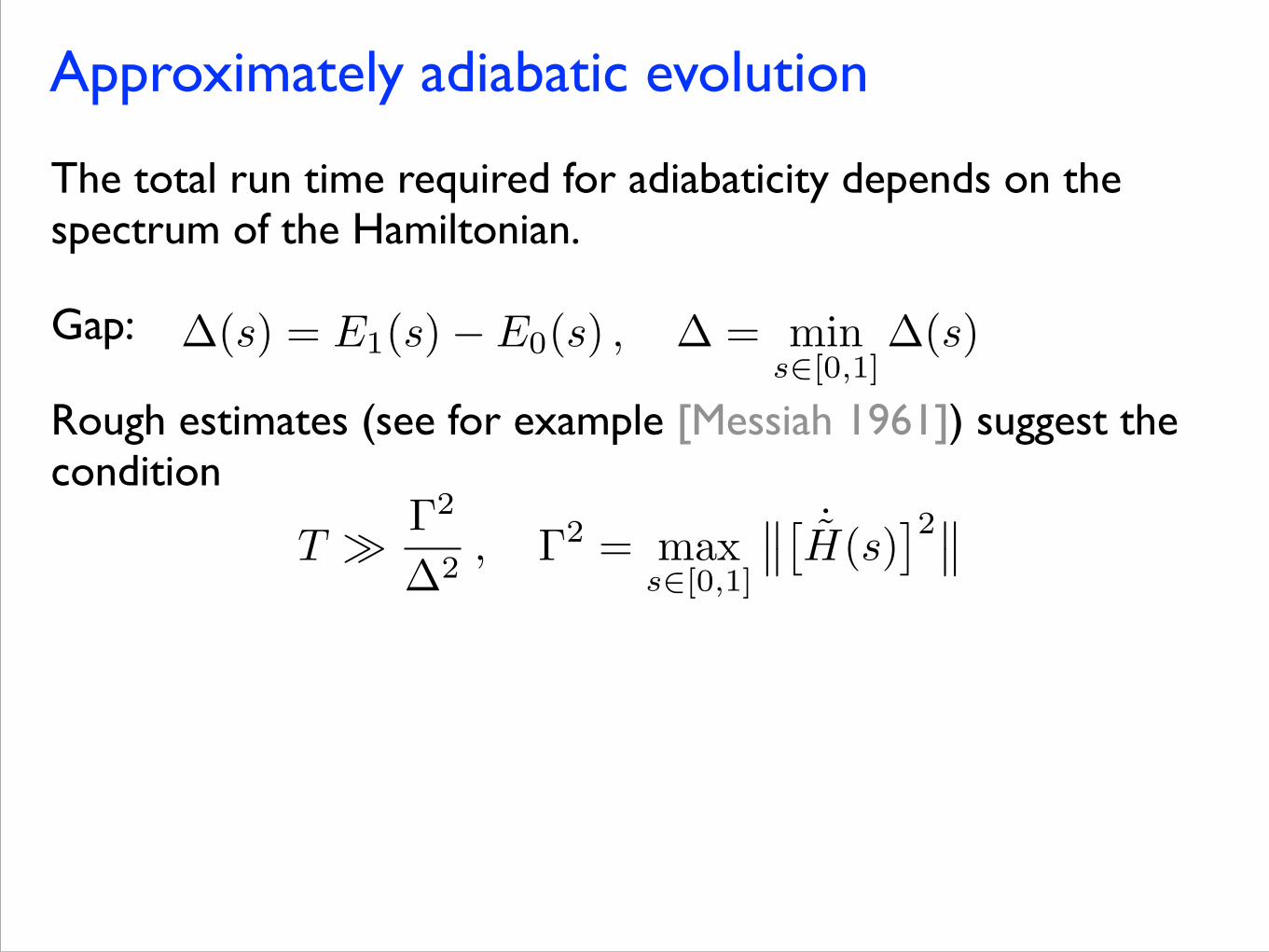
The total run time required for adiabaticity depends on the spectrum of the Hamiltonian.
Gap:
Rough estimates (see for example [Messiah 1961]) suggest the condition
T � �
2
�
2, �
2= max
s2[0,1]
��⇥˙
˜H(s)⇤2��
�(s) = E1(s)� E0(s) , � = mins2[0,1]
�(s)
Approximately adiabatic evolution
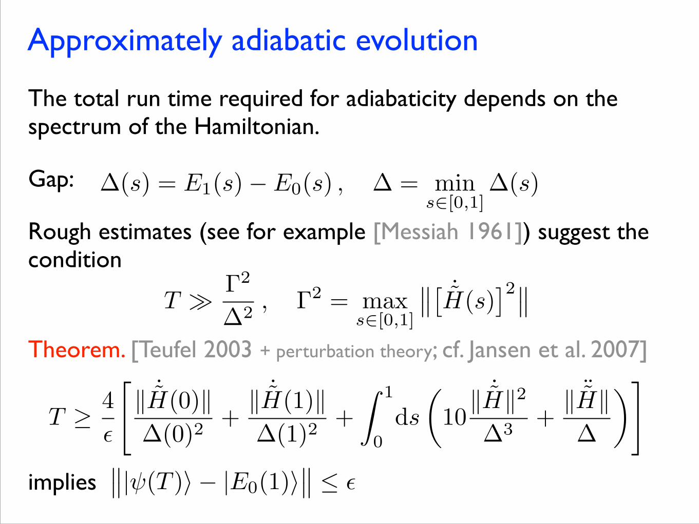
The total run time required for adiabaticity depends on the spectrum of the Hamiltonian.
Gap:
Rough estimates (see for example [Messiah 1961]) suggest the condition
!
Theorem. [Teufel 2003 + perturbation theory; cf. Jansen et al. 2007]
!
implies��| (T )i � |E0(1)i
�� ✏
T � �
2
�
2, �
2= max
s2[0,1]
��⇥˙
˜H(s)⇤2��
�(s) = E1(s)� E0(s) , � = mins2[0,1]
�(s)
T � 4✏
"k ˙̃H(0)k�(0)2
+k ˙̃H(1)k�(1)2
+Z 1
0ds
✓10k ˙̃Hk2
�3+k ¨̃Hk�
◆#
Satisfiability problems
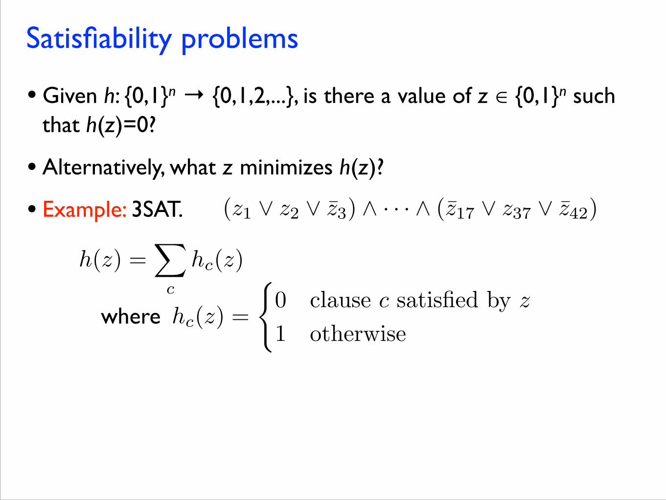
• Given h: {0,1}n → {0,1,2,...}, is there a value of z ∈ {0,1}n such that h(z)=0?
• Alternatively, what z minimizes h(z)?
• Example: 3SAT. where
(z1 _ z2 _ z̄3) ^ · · · ^ (z̄17 _ z37 _ z̄42)
h(z) =X
c
hc(z)
hc(z) =
(0 clause c satisfied by z
1 otherwise
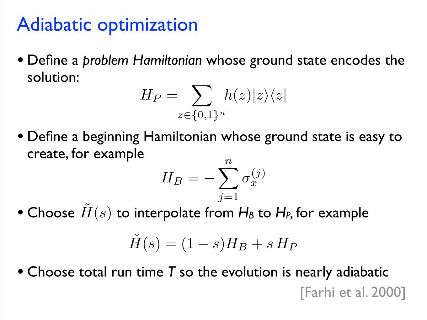
Adiabatic optimization
• Define a problem Hamiltonian whose ground state encodes the solution:
!
• Define a beginning Hamiltonian whose ground state is easy to create, for example
!
• Choose to interpolate from HB to HP, for example
!
• Choose total run time T so the evolution is nearly adiabatic
H̃(s)
H̃(s) = (1� s)HB + sHP
HP =X
z2{0,1}n
h(z)|zihz|
HB
= �nX
j=1
�(j)x
[Farhi et al. 2000]
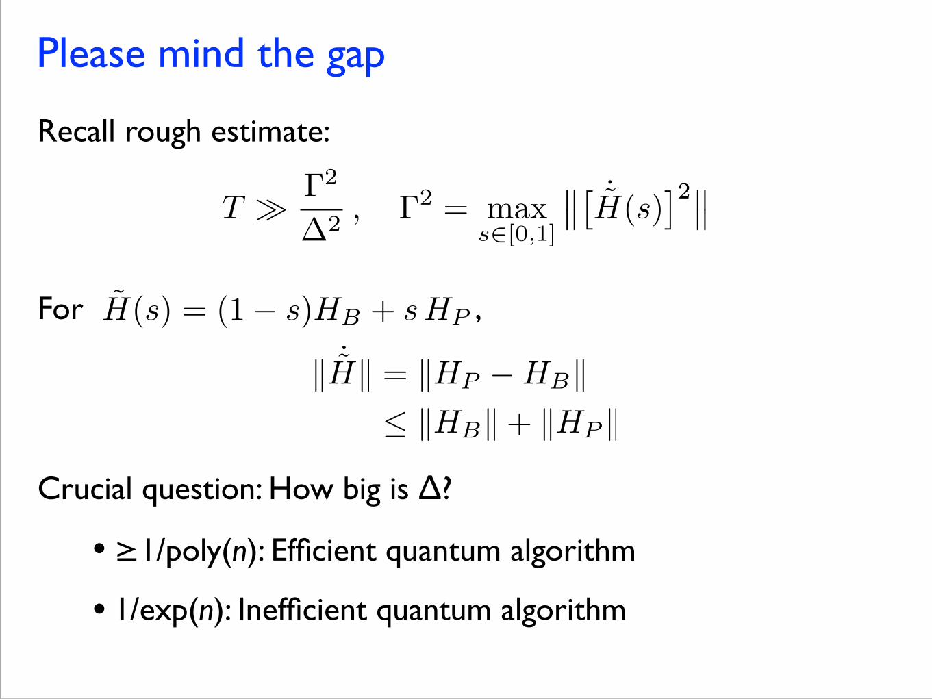
Please mind the gap
Recall rough estimate:
!
!
For ,
!
!
Crucial question: How big is Δ?
•≥1/poly(n): Efficient quantum algorithm
• 1/exp(n): Inefficient quantum algorithm
T � �
2
�
2, �
2= max
s2[0,1]
��⇥˙
˜H(s)⇤2��
H̃(s) = (1� s)HB + sHP
� ˙̃H� = �HP �HB�� �HB�+ �HP �
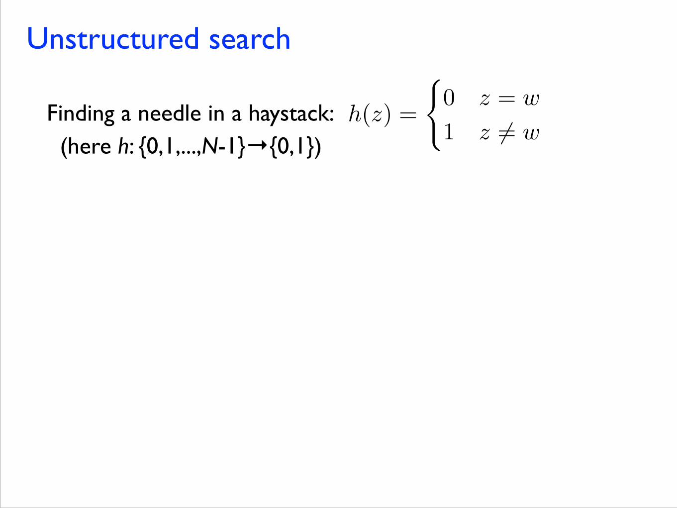
Unstructured search
Finding a needle in a haystack: (here h: {0,1,...,N-1}→{0,1})
h(z) =
(0 z = w
1 z 6= w
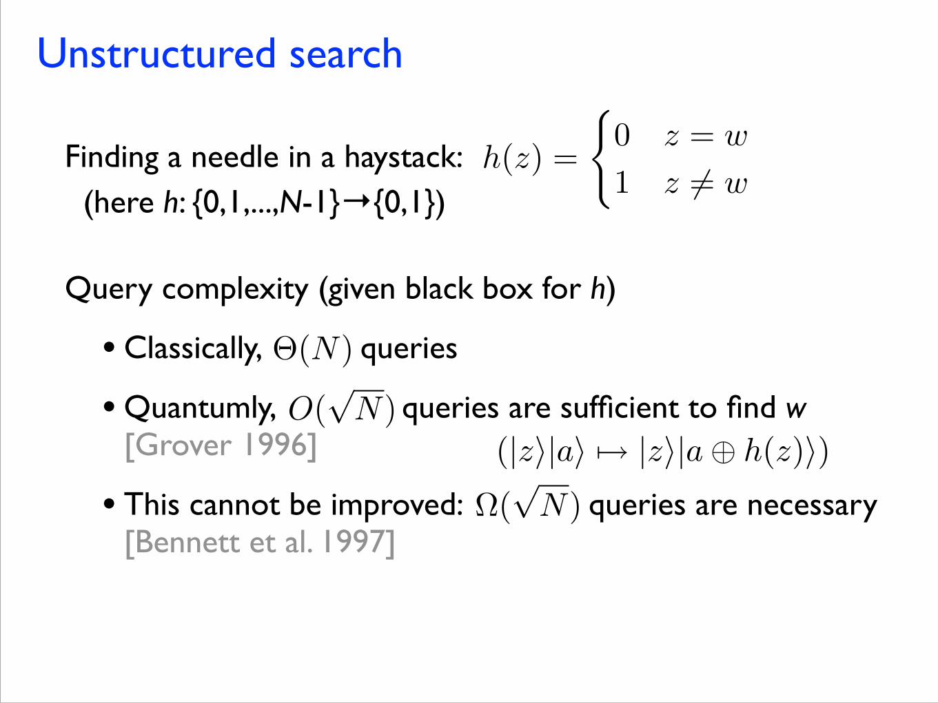
Unstructured search
Finding a needle in a haystack: (here h: {0,1,...,N-1}→{0,1}) !
Query complexity (given black box for h)
• Classically, queries
• Quantumly, queries are sufficient to find w [Grover 1996]
• This cannot be improved: queries are necessary [Bennett et al. 1997]
⇥(N)
O(p
N)
⌦(p
N)
h(z) =
(0 z = w
1 z 6= w
(|zi|ai 7! |zi|a� h(z)i)
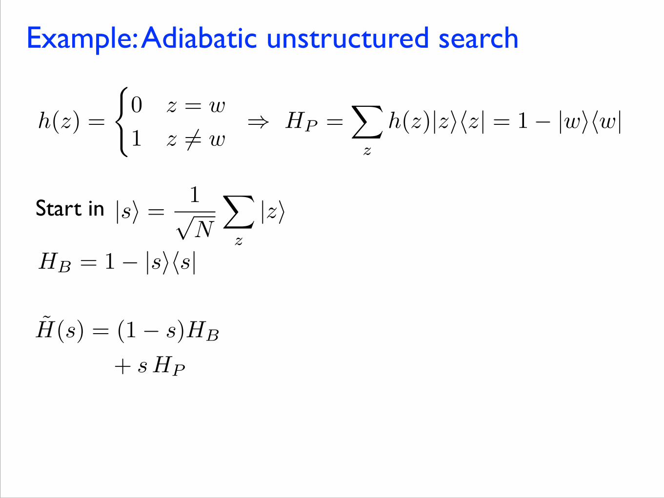
Example: Adiabatic unstructured search
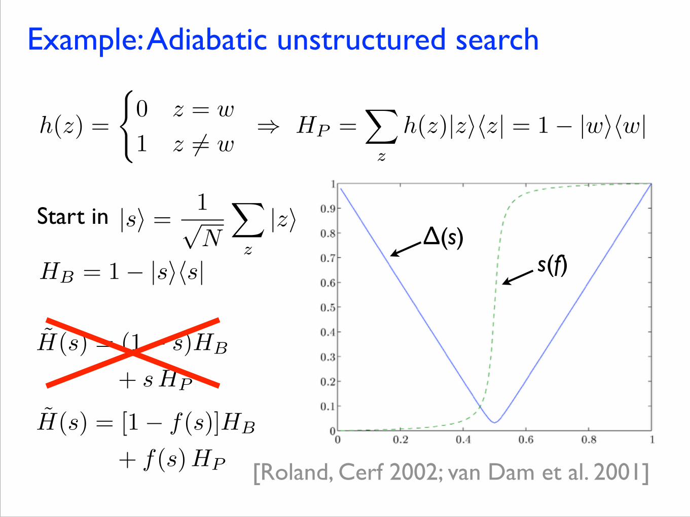
h(z) =
(0 z = w
1 z 6= w) HP =
X
z
h(z)|zihz| = 1� |wihw|
HB = 1 � |sihs|
|si =1pN
X
z
|ziStart in
H̃(s) = (1� s)HB
+ sHP
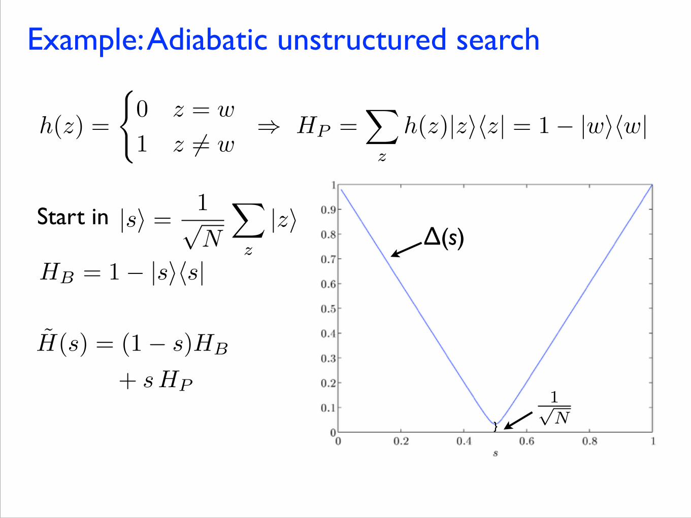
Example: Adiabatic unstructured search
h(z) =
(0 z = w
1 z 6= w) HP =
X
z
h(z)|zihz| = 1� |wihw|
HB = 1 � |sihs|
|si =1pN
X
z
|ziStart in
H̃(s) = (1� s)HB
+ sHP
Δ(s)
1pN}

Example: Adiabatic unstructured search
h(z) =
(0 z = w
1 z 6= w) HP =
X
z
h(z)|zihz| = 1� |wihw|
HB = 1 � |sihs|
|si =1pN
X
z
|ziStart in
H̃(s) = (1� s)HB
+ sHP
Δ(s)
1pN
1pN
}
}
Example: Adiabatic unstructured search
h(z) =
(0 z = w
1 z 6= w) HP =
X
z
h(z)|zihz| = 1� |wihw|
HB = 1 � |sihs|
|si =1pN
X
z
|ziStart in
H̃(s) = (1� s)HB
+ sHP
H̃(s) = [1� f(s)]HB
+ f(s) HP
Δ(s)s(f)
[Roland, Cerf 2002; van Dam et al. 2001]
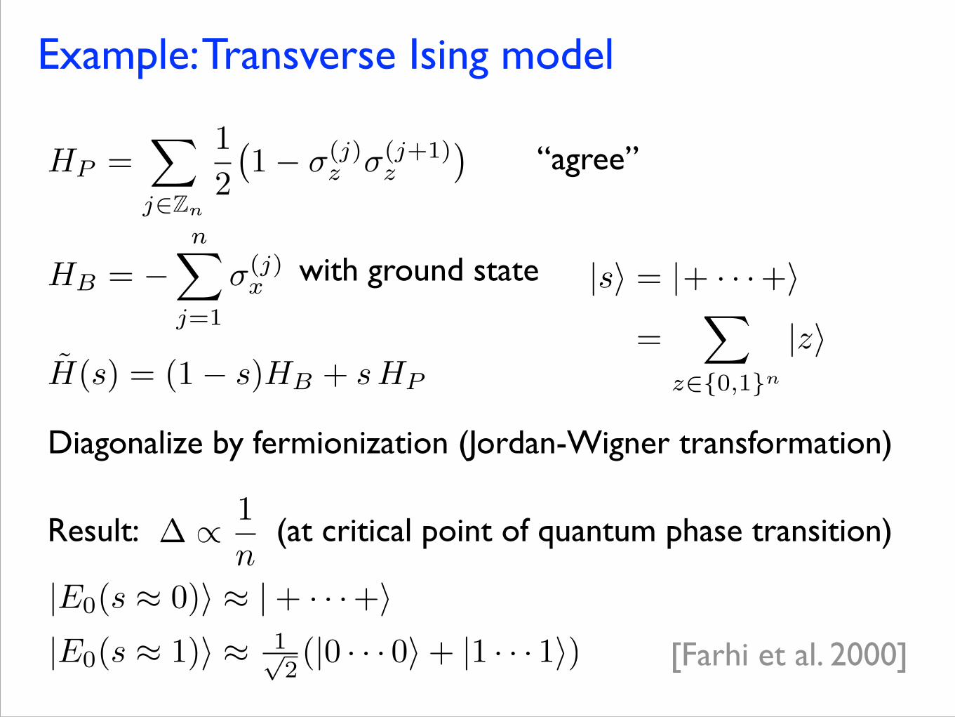
Example: Transverse Ising model
HB
= �nX
j=1
�(j)x
H̃(s) = (1� s)HB + sHP
Diagonalize by fermionization (Jordan-Wigner transformation)
Result: (at critical point of quantum phase transition)� / 1n
“agree”
with ground state
[Farhi et al. 2000]
|E0(s � 0)� � | + · · · +�|E0(s � 1)� � 1�
2(|0 · · · 0�+ |1 · · · 1�)
|s� = |+ · · · +�
=�
z�{0,1}n
|z�
HP =X
j2Zn
12�1� �(j)
z �(j+1)z
�
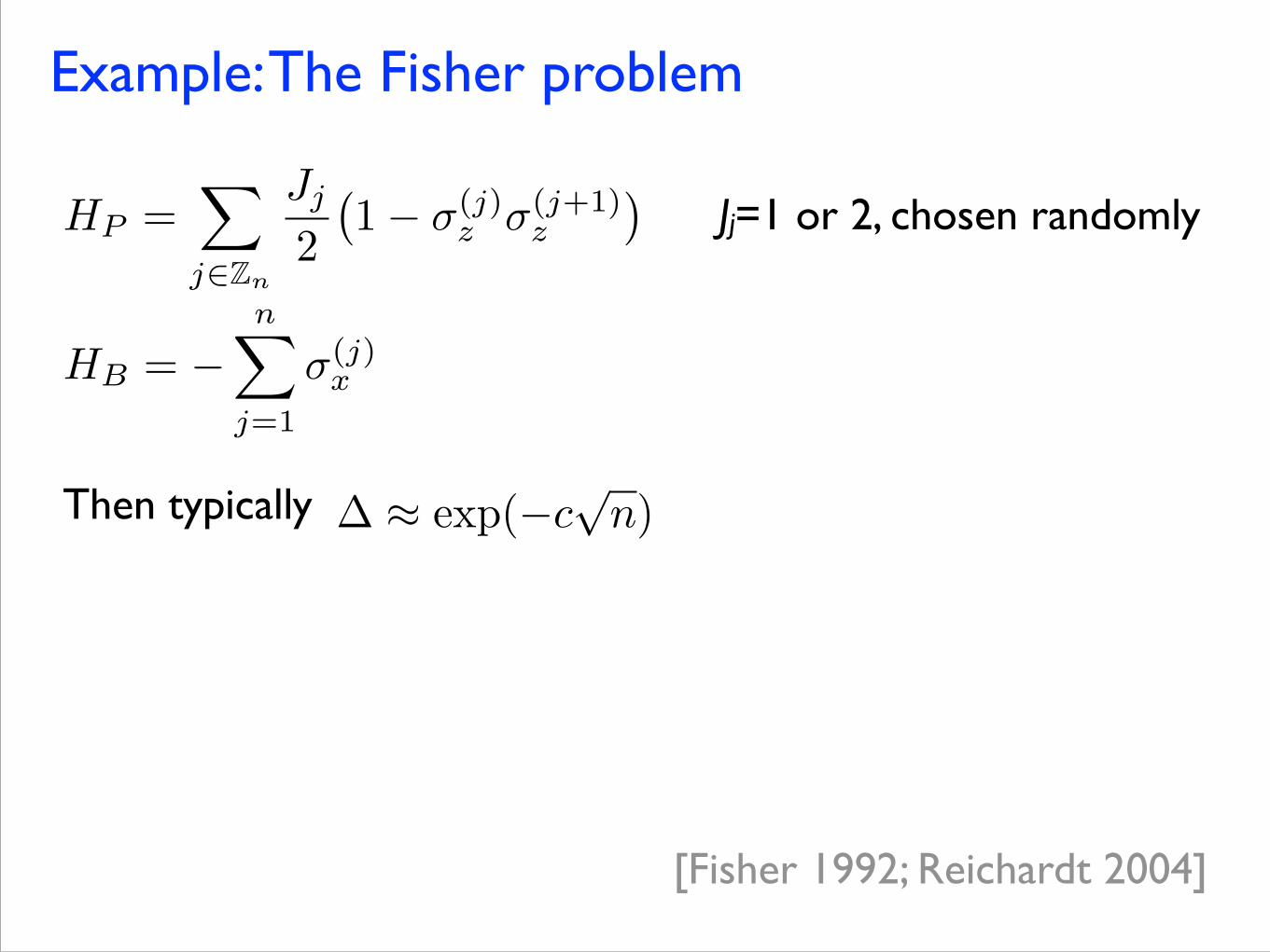
Example: The Fisher problem
[Fisher 1992; Reichardt 2004]
HB
= �nX
j=1
�(j)x
Jj=1 or 2, chosen randomly
Then typically� ⇡ exp(�c
pn)
HP =X
j2Zn
Jj
2�1� �(j)
z �(j+1)z
�
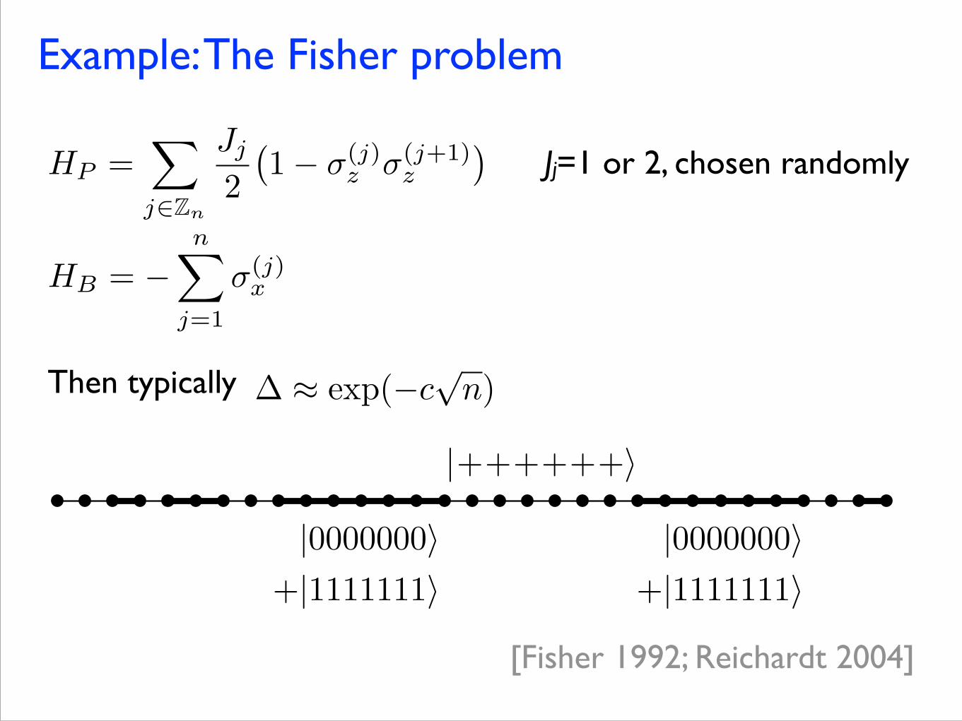
Example: The Fisher problem
[Fisher 1992; Reichardt 2004]
HB
= �nX
j=1
�(j)x
Jj=1 or 2, chosen randomly
Then typically� ⇡ exp(�c
pn)
|0000000�+|1111111�
|++++++�
|0000000�+|1111111�
HP =X
j2Zn
Jj
2�1� �(j)
z �(j+1)z
�
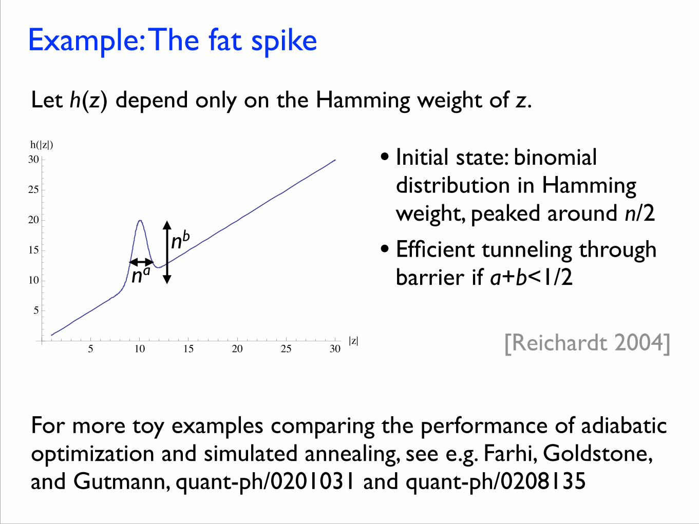
Example: The fat spike
For more toy examples comparing the performance of adiabatic optimization and simulated annealing, see e.g. Farhi, Goldstone, and Gutmann, quant-ph/0201031 and quant-ph/0208135
[Reichardt 2004]
Let h(z) depend only on the Hamming weight of z.
5 10 15 20 25 30»z»
5
10
15
20
25
30hH»z»L
• Initial state: binomial distribution in Hamming weight, peaked around n/2
• Efficient tunneling through barrier if a+b<1/2na
nb

Random satisfiability problems
Consider random instances of some satisfiability problem (e.g. 3SAT, Exact cover, ...) with a fixed ratio of clauses/bits.
Few clauses: underconstrained. Many solutions, easy to find. Many clauses: overconstrained. No solutions, easy to find a contradiction.

Random satisfiability problems
Consider random instances of some satisfiability problem (e.g. 3SAT, Exact cover, ...) with a fixed ratio of clauses/bits.
Few clauses: underconstrained. Many solutions, easy to find. Many clauses: overconstrained. No solutions, easy to find a contradiction.
Simulation results for random exact cover instances with unique satisfying assignments:
8 E. Farhi, J. Goldstone, S. Gutmann, J. Lapan, A. Lundgren, D. Preda
10 11 12 13 14 15 16 17 18 19 20
Number of Bits
0
5
10
15
20
25
30
35
40
45
50
55
60
Med
ian
Tim
e to
Get
Pro
bab
ilit
y 1
/8
New Quadratic Fit
Old Quadratic Fit
Figure 1: Each circle is the median time to achieve a success probability of 1/8 for 75 gusa
instances. The error bars give 95% confidence limits for each median. The solid line is a quadraticfit to the data. The broken line, which lies just below the solid line, is the quadratic fit obtainedin [6] for an independent data set up to 15 bits.
each instance with T = T (n). In Figure 2 the circles show the median probability of successat each n. Not surprisingly, these are all close to 1/8. We also show the tenth-worst andworst probability for each n. The good news for the quantum algorithm is that these do notappear to decrease appreciably with n.
To further explore this we generate 1000 new gusa instances of Exact Cover at both16 and 17 bits. In Figure 3 we show the histograms of the success probability when theinstances are run at T (16) and T (17), respectively. The histograms indicate that a gusa
instance with success probability at or below 0.04 is very unlikely.If an algorithm (classical or quantum) succeeds with probability at least p, then running
the algorithm k times gives a success probability of at least 1 − (1 − p)k. For example, ifp = 0.04, then 200 repetitions of the algorithm gives a success probability of better than0.9997. Suppose that as the number of bits increases it remains true that almost all gusa
instances have a success probability of at least 0.04 at the quadratic run time T (n). Thenany n-independent desired probability of success can be achieved with a fixed number ofrepetitions.
11 Instances with the number of clauses fixed in advance
To study the performance of the quantum algorithm on instances that do not necessarilyhave a usa, we generate new instances now by fixing the number of clauses in advance.Instances are generated with a fixed number of randomly chosen clauses and then separatedinto two categories, those with at least one satisfying assignment and those with none. Both
[Farhi et al. 2001]
Robustness of adiabatic QC
• Unitary control error
• Dephasing in instantaneous eigenstate basis
• Transitions between instantaneous eigenstates: thermal noise
Potential sources of error:
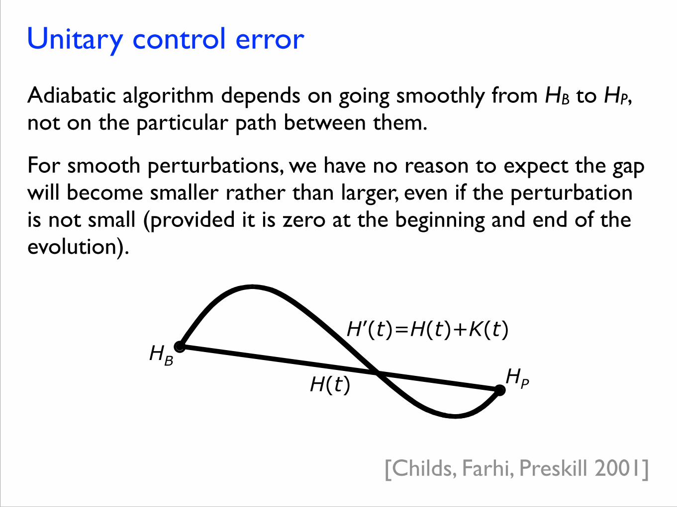
Unitary control error
Adiabatic algorithm depends on going smoothly from HB to HP, not on the particular path between them.
For smooth perturbations, we have no reason to expect the gap will become smaller rather than larger, even if the perturbation is not small (provided it is zero at the beginning and end of the evolution).
H(t)HB
HP
H’(t)=H(t)+K(t)
[Childs, Farhi, Preskill 2001]
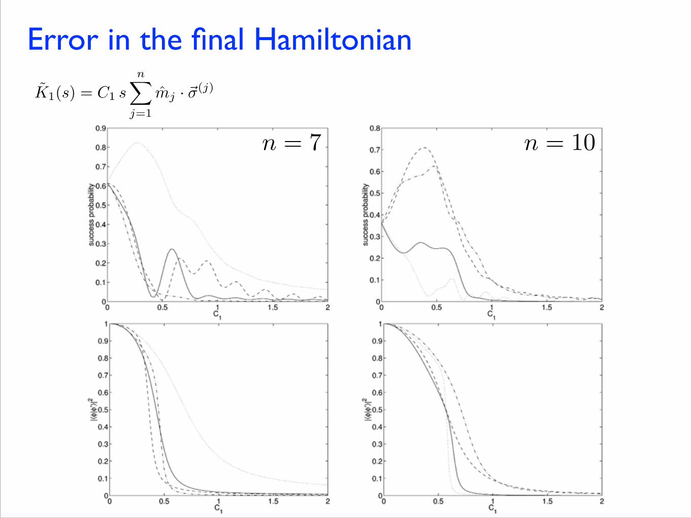
Error in the final Hamiltonian
K̃1(s) = C1 snX
j=1
m̂j · ~�(j)
n = 7 n = 10
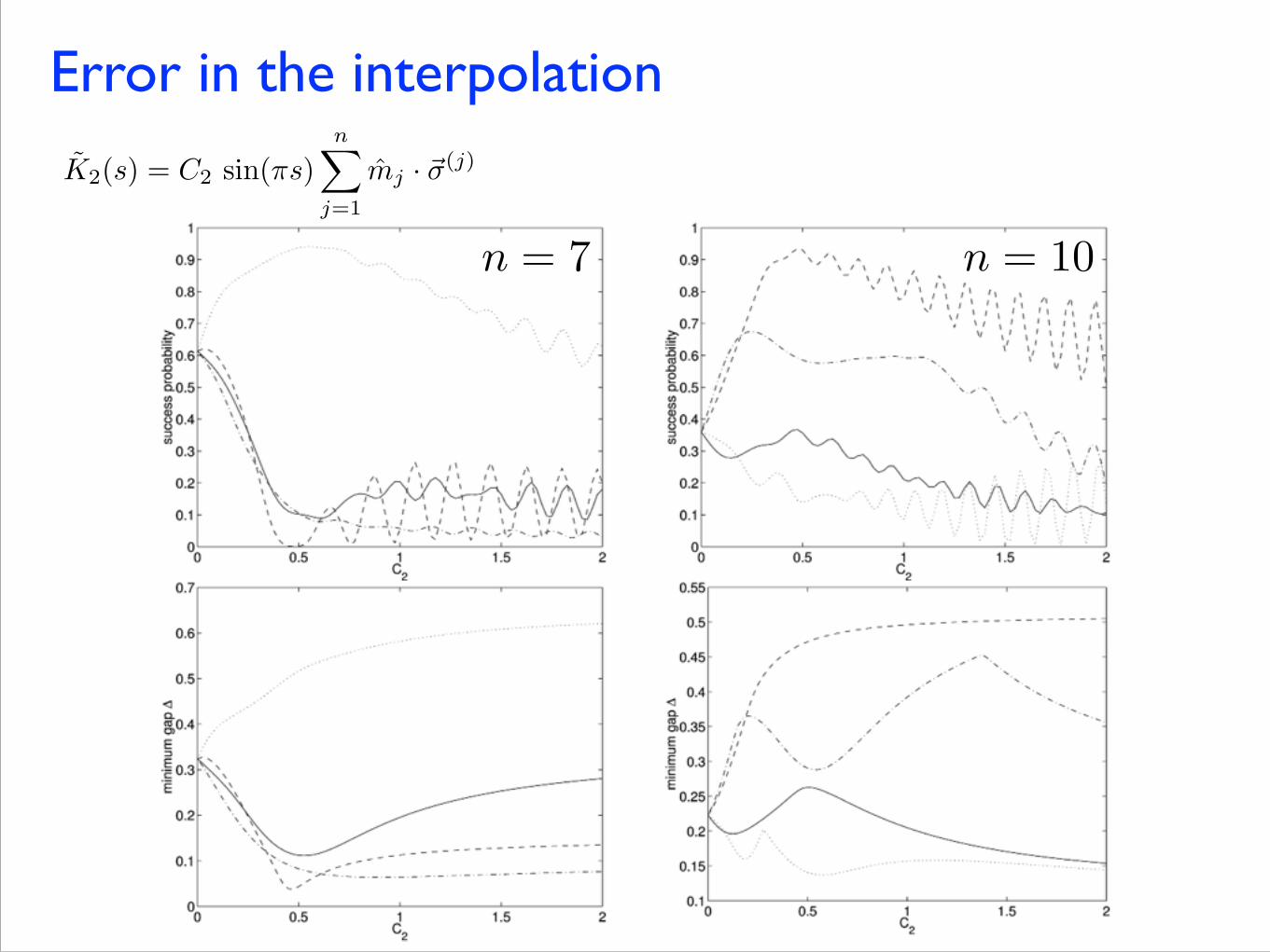
Error in the interpolation
n = 7 n = 10
K̃2(s) = C2 sin(⇡s)nX
j=1
m̂j · ~�(j)

K̃3(s) =12
sin(C3⇡s)nX
j=1
m̂j · ~�(j)
High frequency error
n = 10n = 8
n = 8 n = 10
Thermal noise
Efficient adiabatic quantum computation requires that the minimum gap Δ is not too small. !Provided kB T << Δ, thermal fluctuations are unlikely to drive the system out of the ground state. So a big gap not only allows for adiabaticity, but also provides protection against thermal noise! !Here it is important that H is the actual Hamiltonian of the of the quantum computer, not just a simulated Hamiltonian. !Even for tractable problems, typical gaps decrease as 1/poly(n), so this may not provide any asymptotic protection in realistic systems.
[Childs, Farhi, Preskill 2001]

Universal quantum computation
Adiabatic evolution with linear interpolation between local beginning and ending Hamiltonians can simulate arbitrary QC. !!
Universal quantum computation
Adiabatic evolution with linear interpolation between local beginning and ending Hamiltonians can simulate arbitrary QC. ![Feynman 1985]: !
H =kX
j=1
[Uj ⌦ |j + 1ihj| + U†j ⌦ |jihj + 1|]
Universal quantum computation
Adiabatic evolution with linear interpolation between local beginning and ending Hamiltonians can simulate arbitrary QC. ![Feynman 1985]: !!Basic idea [Aharonov et al. 2004]: Use this as -HP. !Final ground state: !HB enforces correct initial state. Add energy penalties to stay in an appropriate subspace.
H =kX
j=1
[Uj ⌦ |j + 1ihj| + U†j ⌦ |jihj + 1|]
1pk
kX
j=1
UjUj�1 · · · U1|0i ⌦ |ji
Universal quantum computation
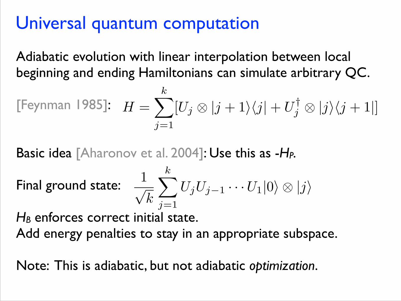
Adiabatic evolution with linear interpolation between local beginning and ending Hamiltonians can simulate arbitrary QC. ![Feynman 1985]: !!Basic idea [Aharonov et al. 2004]: Use this as -HP. !Final ground state: !HB enforces correct initial state. Add energy penalties to stay in an appropriate subspace. !Note: This is adiabatic, but not adiabatic optimization.
H =kX
j=1
[Uj ⌦ |j + 1ihj| + U†j ⌦ |jihj + 1|]
1pk
kX
j=1
UjUj�1 · · · U1|0i ⌦ |ji
Open questions: Stoquastic Hamiltonians
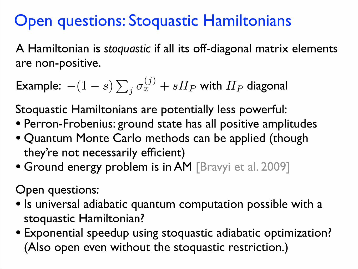
A Hamiltonian is stoquastic if all its off-diagonal matrix elements are non-positive.
Example: with diagonal�(1� s)P
j
�(j)x
+ sHP
HP
Stoquastic Hamiltonians are potentially less powerful: • Perron-Frobenius: ground state has all positive amplitudes • Quantum Monte Carlo methods can be applied (though
they’re not necessarily efficient) • Ground energy problem is in AM [Bravyi et al. 2009]
Open questions: • Is universal adiabatic quantum computation possible with a
stoquastic Hamiltonian? • Exponential speedup using stoquastic adiabatic optimization?
(Also open even without the stoquastic restriction.)
Open questions: Fault tolerance
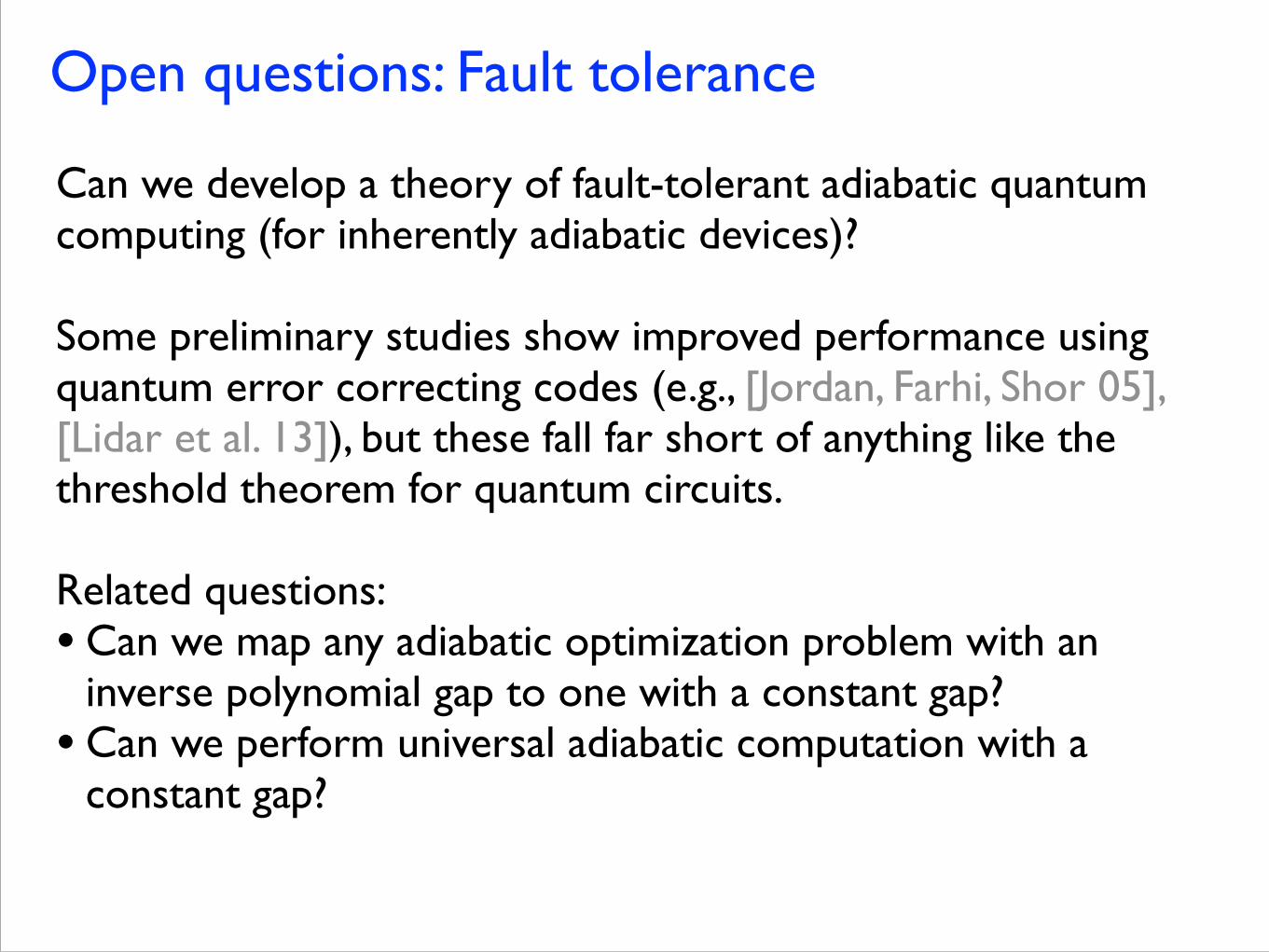
Can we develop a theory of fault-tolerant adiabatic quantum computing (for inherently adiabatic devices)?
Some preliminary studies show improved performance using quantum error correcting codes (e.g., [Jordan, Farhi, Shor 05], [Lidar et al. 13]), but these fall far short of anything like the threshold theorem for quantum circuits.
Related questions: • Can we map any adiabatic optimization problem with an
inverse polynomial gap to one with a constant gap? • Can we perform universal adiabatic computation with a
constant gap?