water

Review

Overview, Comparative Assessment andRecommendations of Forecasting Models forShort-Term Water Demand Prediction

Amos O. Anele 1,*, Yskandar Hamam 1, Adnan M. Abu-Mahfouz 1,2 ID and Ezio Todini 3

1 Department of Electrical Engineering, Tshwane University of Technology, Pretoria 0001, South Africa;hamama@tut.ac.za (Y.H.); AAbuMahfouz@csir.co.za (A.M.A.-M.)

2 Council for Scientific and Industrial Research, Pretoria 0081, South Africa3 Department of Biological, Geological and Environmental Sciences, University of Bologna, Via Zamboni,

33-40126 Bologna, Italy; eziotodini@gmail.com* Correspondence: anelea@tut.ac.za or aneleamos@gmail.com; Tel.: +27-12-382-4191

Received: 8 September 2017; Accepted: 6 November 2017 ; Published: 13 November 2017

Abstract: The stochastic nature of water consumption patterns during the day and week varies.Therefore, to continually provide water to consumers with appropriate quality, quantity andpressure, water utilities require accurate and appropriate short-term water demand (STWD) forecasts.In view of this, an overview of forecasting methods for STWD prediction is presented. Based onthat, a comparative assessment of the performance of alternative forecasting models from thedifferent methods is studied. Times series models (i.e., autoregressive (AR), moving average (MA),autoregressive-moving average (ARMA), and ARMA with exogenous variable (ARMAX)) introducedby Box and Jenkins (1970), feed-forward back-propagation neural network (FFBP-NN), and hybridmodel (i.e., combined forecasts from ARMA and FFBP-NN) are compared with each other for acommon set of data. Akaike information criterion (AIC), originally proposed by Akaike (1974) is usedto estimate the quality of each short-term forecasting model. Furthermore, Nash–Sutcliffe (NS) modelefficiency coefficient proposed by Nash–Sutcliffe (1970), root mean square error (RMSE) and meanabsolute percentage error (MAPE) are the forecasting statistical terms used to assess the predictiveperformance of the models. Lastly, as regards the selection of an accurate and appropriate STWDforecasting model, this paper provides recommendations and future work based on the forecastsgenerated by each of the predictive models considered.

Keywords: forecasting models; short-term; water demand simulation

1. Introduction

The most crucial factor in the planning, operation and management of water distribution systems(WDS) is the satisfaction of consumer demand. The stochastic nature of water demand during the dayand week is influenced by several factors; namely, climatic and geographic conditions, commercial andsocial conditions of people, population growth, industrialisation, technical innovation, cost of supply,and condition of WDS [1–4]. Therefore, water utilities need accurate and appropriate short-term waterdemand (STWD) forecasts in order to continually satisfy consumers with quality water in adequatevolumes, and at reasonable pressures [5–7]. STWD forecasting is an important component of thesuccessful operation, management, and optimisation of any existing WDS. As a result, the selection ofan accurate and appropriate STWD forecasting model is useful for [1,6,8–16]:

• explaining day-to-day demand variations• minimising the operating cost of pumping stations• pinpointing possible network failures (e.g., water leaks and pipe bursts)

Water 2017, 9, 887; doi:10.3390/w9110887 www.mdpi.com/journal/water

Water 2017, 9, 887 2 of 12

• helping utilities plan and manage water demands for near-term events• optimizing daily operations of the infrastructure (e.g., pump scheduling, control of reservoirs

volume, pressure management, and water conservation program)

In the light of the above, the first objective of this paper is to present an overview of forecastingmethods for STWD prediction. Based on that, the second objective is to conduct a comparativeassessment of the performance of alternative forecasting models from the different methods. As regardsthe selection of an accurate and appropriate model, the third objective of the paper is to presentrecommendations and future work for the forecasts generated by the forecasting models considered.

2. Overview of STWD Forecasting Methods

In this section, the overview of univariate time series (UTS), time series regression (TSR), artificialneural network (ANN), and hybrid methods for STWD prediction is presented (see also Table 1).

2.1. UTS Forecasting Methods

UTS methods forecast future water demand based on past observations and associatederror terms [17,18]. Exponential smoothing, autoregressive (AR), moving average (MA),autoregressive-moving average (ARMA), autoregressive integrated moving average (ARIMA) andseasonal ARIMA (SARIMA) are examples of UTS forecasting models. These models are useful forshort-term operational forecasts. However, they may not be the most accurate alternative when weatherchanges are likely to occur in the underlying determinants of water demands [11,18]. Furthermore,it is discussed in [11] that stochastic process models (i.e., AR, MA, ARMA, and ARIMA) are used sinceexponential smoothing models sometimes cease to be adequate when time series data exhibit morecomplex profiles. Based on that, to achieve the second objective of this paper, the model processes ofAR(p), MA(q), and ARMA(p, q) are respectively considered as given in Equations (1)–(3) [17,18].

Yt = µ +p

∑k=1

φkYt−k + εt (1)

Yt = µ + εt +q

∑k=1

θkεt−k (2)

Yt = µ +p

∑k=1

φkYt−k + εt +q

∑k=1

θkεt−k (3)

where p and q are the model orders, φ is the autoregressive parameter, θ is the moving averageparameter, µ is the mean value of the process, and εt is the forecast error at time t. Yt is the observedvalue of demand at time t, k is the number of historical periods, Yt−k and εt−k are the observation attime t−k.

2.2. Time Series Regression (TSR) Forecasting Methods

Unlike the UTS models, TSR forecasting models consider the effects of exogenous variables.This is because they generate forecasts based on the relationship between water demand and itsdeterminants [19–21]. TSR models include multiple linear regression (MLR), multiple and nonlinearregression (MNLR), ARMA with exogenous variable (ARMAX) and ARIMA with exogenous variable(ARIMAX). Among others, the ARMAX(p, q, b) model is considered to achieve the second objective ofthis paper. Equation (4) is useful in a case where the demand at time t is influenced by MA and ARterms, in addition to exogenous variables and their autoregressive terms [11].

Yt = µ +p

∑k=1

φkYt−k + εt +q

∑k=1

θkεt−k +b

∑k=0

βkxt−k (4)

Water 2017, 9, 887 3 of 12

where b is a single exogenous variable considered for the ARMAX model. Additionally, βk and xt−kare respectively the coefficient and observed value of the kth independent variable.

2.3. Artificial Neural Network (ANN) Forecasting Methods

ANNs were introduced following Rosenblatt’s concept of perceptron [22], and their applicationusually involves a comparative assessment of the performance with TSR models (e.g., feed-forwardback-propagation neural network (FFBP-NN), generalized regression neural networks (GRNNs),radial basis neural networks (RBNNs), and MLR) [1,10,23–26], with UTS models (e.g., dynamicartificial neural network (DAN2), ARIMA and FFBP-NN) [27] or with both UTS and TSR models(e.g., simple linear regression (SLR), MLR, UTS models, and ANN models) [5,28,29]. Nonetheless, inorder to achieve the second objective of this paper, FFBP-NN (see Equation (5)) is considered [1].

Yt = α0 +p

∑j=1

αj f (h

∑i=1

βijYt−j + β0j) + εt (5)

where p is the number of hidden nodes, h is the number of input nodes, f is a sigmoid transfer function,αj is the vector of the weights from hidden to the output nodes, βij are the weights from the input tohidden nodes, and α0 and β0j are the weights of the arcs leaving from the bias terms.

2.4. Hybrid Forecasting Methods

Forecasting with hybrid models (i.e., combined forecasts from two or more predictive models) hasfound wide application [6,11,24,30–34], since it leads to better forecasting performance. For instance,Equation (6) is applied in a case where forecasts from different models are combined in order to obtaina hybrid forecast. As regards achieving the second objective of this paper, the combined forecast isobtained by using a UTS model (i.e., ARMA) and an ANN model (i.e., FFBP-NN).

Yt = β0 +n

∑i=1

βiYi,t (6)

where Yi,t is the predicted value of the time series at time t using the ith model, β0 is the regressionintercept, βi coefficients are determined by optimisation or least squares regression to minimise themean square error (MSE) between the hybrid forecast Yi,t and the actual data [11].

Water 2017, 9, 887 4 of 12

Table 1. Brief summary of short-term water demand (STWD) forecasting methods and models. UTS: univariate time series; MA: moving average; AR: autoregressive;ARIMA: autoregressive integrated moving average; ARMA: autoregressive-moving average; SARIMA: seasonal ARIMA; TSR: time series regression; MNLR: multipleand nonlinear regression; ARMAX: ARMA with exogenous variable; MLR: multiple linear regression; ARIMAX: ARIMA with exogenous variable; ANN: artificialneural network; FFBP-NN: feed-forward back-propagation neural network; GRNN: generalized regression neural network; RBNN: radial basis neural network;DAN2: dynamic artificial neural network; GARCH: generalized autoregressive conditional heteroskedasticity.

Forecasting Methods and Models Quantitative Assessment of Forecast Accuracy Forecast Purpose

UTS models [18,27,29]: MA, AR, ARIMA,exponential smoothing, ARMA, SARIMA

It can exhibit more complex profiles. However, it does notaccount for the effect of exogenous variables (e.g., weatherdata or price) [11].

Useful for short-term operational forecasts (i.e., tominimise the operating cost of pumping stations, etc.)

TSR models [1,25,26]: MNLR, ARMAX,MLR and ARIMAX

TSR models produce forecasts on the basis of therelationship between water demand and its determinants(e.g., weather data, income, demographics) [19].

Useful for better prediction of daily waterdemand [24]. Relevant for setting water rates, revenueforecasting, and financial planning exercises.

ANN models: FFBP-NN, GRNN, RBNN,DAN2 [5,35]

Used with TSR models [1,24–27], with UTS models [27],or with both UTS and TSR models [5,28,29]. Accordingto [11], ANN outperforms UTS and TSR models.However, the results of [24,25] were inconclusive.

Useful for a better prediction of peak daily water demand.To inform optimal operating policy as well as pumpingand maintenance scheduling.

Hybrid models: FFBP-NN and AR [36],Holt–Winters, ARIMA, and GARCH [37],Fuzzy logic and AR [38]

Different forecasting models are able to capture differentaspects of the information available forprediction [11]. As a result, leading to better forecastingperformance [33,36]

Useful for real-time, near-optimal control of waterdistribution systems (WDS) [6]. Necessary for operationalpurposes [33,36].

Water 2017, 9, 887 5 of 12

3. Presentation and Discussion of Results

In this paper, ARIMA-based models (i.e., AR, MA, ARMA, ARMAX) together with the widelyused non-parametric forecasting model, FFBP-NN, have been compared with each other and againstthe hybrid model, a combination of two or more forecasting models (i.e., ARMA and FFBP-NN) for acommon set of data (see Figure 1). Figure 1a shows the average water consumption for the 24 h of eachday for a city in south-eastern Spain, obtained from all the available data provided in [1]. The predictivemodels considered in this paper were used to forecast hourly water demands. In addition, an averageweekly data of 168 h was used, and based on that, the proportion of data used for the training andtesting were 60% and 40% respectively.

Figure 1a shows a similar behaviour during the early morning (e.g., all curves grow from 6:00 a.m.until 10:00 a.m.). In addition, from 10:00 a.m. to 4:00 p.m., all the curves have decreasing and increasingtrend (except on weekends). According to [1], temperature is said to be the main factor that influencesmultiple sources of water consumption (e.g., showers, water for garden, etc.). Hence, Figure 1b showsthe single exogenous variable considered for ARMAX model.

The results shown in Figures 2–5 are obtained by computing Equations (1)–(6) in MATLAB.Figures 2–4 show the forecasts generated by AR and MA (see Figure 2), ARMA and ARMAX(see Figure 3), as well as FFBP-NN and hybrid model (see Figure 4). Figure 5a–c show the comparativeassessment of the predictive performance of these models by using forecasting statistical terms such asroot mean square error (RMSE), mean absolute percentage error (MAPE), and Nash–Sutcliffe (NS) [39].This assessment was achieved by computing Equations (7)–(9). In addition, the estimate of the relativequality of AR, MA, ARMA, ARMAX, and FFBP-NN is shown in Figure 5d, and it was obtained byapplying Akaike information criterion (AIC) [40], which is based on Equation (10). The forecastspresented in this paper were generated using the best model order, which is determined by the AIC.

Hour of the day [h]0 5 10 15 20 25

Ave

rage

wat

er c

onsu

mpt

ion

[m3]

5

10

15

20

25

30

35

MondayTuesdayWednesdayThursdayFridaySaturdaySunday

(a)Time of the Week [h]

0 20 40 60 80 100 120 140 160 180

Rel

ativ

e te

mpe

artu

re

0.42

0.425

0.43

0.435

0.44

0.445

0.45

0.455

0.46

0.465

0.47

(b)

Figure 1. (a) Daily water demand profile and (b) Single exogenous variable “relative temperature”.

Figures 2a,c, 3a,c, and 4a,c were obtained by using the training dataset, whereas the test datasetwas used to obtain Figures 2b,d, 3b,d, and 4b,d. Based on the application of AIC [40], Figure 2a,bshow that a model process of AR(p = 2) was used to generate the forecasts for the training and testdatasets. A model process of MA(q = 3) was also used to obtain the forecasts presented in Figure 2c,d.The forecasts shown in Figure 3a,b were obtained based on a model process of ARMA(p = 1, q = 1).The results of Figure 3c,d were obtained using a model process of ARMAX(p = 1, q = 1, b = 1).A model order of three was used to obtain the results shown in Figure 4a,b. The configuration of theneural network was achieved with a feed-forward neural network of one hidden layer (10 hiddenneurons) using a Levenberg–Marquardt optimisation-based backpropagation algorithm to train theneural network weights. The training was stopped using validation data (15% of the training datasets).This process was performed 10 times (i.e., 10 cross-validation) to select the feed-forward neural network

Water 2017, 9, 887 6 of 12

with the best predictive accuracy to compensate for neural network training variations. The modelorders mentioned in this paper are the best, and were obtained using AIC. Lastly, the optimal weightingof the hybrid forecast obtained using ARMA and FFBP-NN—as shown in Figure 4c,d—was achievedby using linear least square optimisation.

Time of the Week [h]0 20 40 60 80 100 120

Ave

rage

Wat

er D

eman

d [m

3]

10

12

14

16

18

20

22

24

26

28AR(2), RMSE = 2.37, MAPE = 10.07% and NS = 0.74

Trained Data ObservationPredicted Data

(a)Time of the Week [h]

100 110 120 130 140 150 160 170

Ave

rage

Wat

er D

eman

d [m

3]

5

10

15

20

25

30

35AR(2), RMSE = 2.67, MAPE = 11.59% and NS = 0.80

Tested Data ObservationPredicted Data

(b)

Time of the Week [h]0 20 40 60 80 100 120

Ave

rage

Wat

er D

eman

d [m

3]

10

12

14

16

18

20

22

24

26

28MA(3), RMSE = 2.46, MAPE = 10.67% and NS = 0.72

Trained Data ObservationPredicted Data

(c)Time of the Week [h]

100 110 120 130 140 150 160 170

Ave

rage

Wat

er D

eman

d [m

3]

5

10

15

20

25

30

35MA(3), RMSE = 2.59, MAPE = 11.42% and NS = 0.81

Tested Data ObservationPredicted Data

(d)

Figure 2. Forecasts generated using (a,b) AR model and (c,d) MA model. The best model orders,AR(p = 2) and MA(q = 3), were determined based on Akaike information criterion (AIC)computation [40]. MAPE: mean absolute percentage error; NS: Nash–Sutcliffe; RMSE: root meansquare error.

The RMSE and MAPE were used to evaluate the forecasting accuracy of the predictivemodels. In addition, NS was used to estimate the forecasting power of the models. The resultsof Figures 2b,d, 3b,d, and 4b,d show that the hybrid model was the best forecasting modelfor STWD prediction (i.e., RMSE = 0.82, MAPE = 3.56%, NS = 0.98) followed by ARMAX(i.e., RMSE = 1.03, MAPE = 3.86%, NS = 0.95), ARMA (i.e., RMSE = 1.85, MAPE = 7.63%, NS = 0.91), MA(i.e., RMSE = 2.59, MAPE = 11.42%, NS = 0.81), AR (i.e., RMSE = 2.67, MAPE = 11.59%, NS = 0.8),and FFBP-NN (i.e., RMSE = 2.8, MAPE = 12.31%, NS = 0.78). In addition, the plots of RMSE, MAPE,and NS versus model order variation are also presented in Figure 5a–c. Compared to AR, MA, ARMA,and FFBP-NN, Figure 5d shows that the AIC value for ARMAX is the smallest. This implies that thequality of the ARMAX model compared to others (i.e., AR, MA, ARMA, and FFBP-NN) is estimated tobe the best. The predictive accuracy of all models decreases as the model order increases. For instance,FFBP-NN model had a remarkable decrease in accuracy compared to other models. Due to theadditional piece of information (i.e., relative temperature) as shown in Figure 1b, the results obtainedin Figures 3 and 5 show that ARMAX(1,1,1) provided a better forecast than ARMA(1,1). Generally,

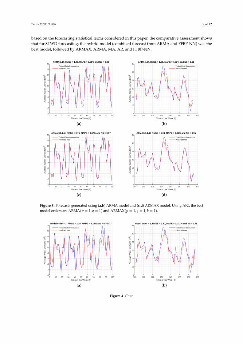
Water 2017, 9, 887 7 of 12

based on the forecasting statistical terms considered in this paper, the comparative assessment showsthat for STWD forecasting, the hybrid model (combined forecast from ARMA and FFBP-NN) was thebest model, followed by ARMAX, ARMA, MA, AR, and FFBP-NN.

Time of the Week [h]0 10 20 30 40 50 60 70 80 90 100

Ave

rage

Wat

er D

eman

d [m

3]

10

12

14

16

18

20

22

24

26

28ARMA(1,1), RMSE = 1.48, MAPE = 6.98% and NS = 0.89

Trained Data ObservationPredicted Data

(a)Time of the Week [h]

100 110 120 130 140 150 160 170

Ave

rage

Wat

er D

eman

d [m

3]

5

10

15

20

25

30

35ARMA(1,1), RMSE = 1.85, MAPE = 7.63% and NS = 0.91

Tested Data ObservationPredicted Data

(b)

Time of the Week [h]0 10 20 30 40 50 60 70 80 90 100

Ave

rage

Wat

er D

eman

d [m

3]

10

12

14

16

18

20

22

24

26

28ARMAX(1,1,1), RMSE = 0.76, MAPE = 3.37% and NS = 0.97

Trained Data ObservationPredicted Data

(c)Time of the Week [h]

100 110 120 130 140 150 160 170

Ave

rage

Wat

er D

eman

d [m

3]

5

10

15

20

25

30

35ARMAX(1,1,1), RMSE = 1.03, MAPE = 3.86% and NS = 0.95

Tested Data ObservationPredicted Data

(d)

Figure 3. Forecasts generated using (a,b) ARMA model and (c,d) ARMAX model. Using AIC, the bestmodel orders are ARMA(p = 1, q = 1) and ARMAX(p = 1, q = 1, b = 1).

Time of the Week [h]0 10 20 30 40 50 60 70 80 90 100

Ave

rage

Wat

er D

eman

d [m

3]

10

12

14

16

18

20

22

24

26

28Model order = 3, RMSE = 2.20, MAPE = 9.28% and NS = 0.77

Trained Data ObservationPredicted Data

(a)Time of the Week [h]

100 110 120 130 140 150 160 170

Ave

rage

Wat

er D

eman

d [m

3]

5

10

15

20

25

30

35Model order = 3, RMSE = 2.80, MAPE = 12.31% and NS = 0.78

Tested Data ObservationPredicted Data

(b)

Figure 4. Cont.

Water 2017, 9, 887 8 of 12

Time of the Week [h]0 10 20 30 40 50 60 70 80 90 100

Ave

rage

Wat

er D

eman

d [m

3]

10

12

14

16

18

20

22

24

26

28RMSE = 0.70, MAPE = 3.21% and NS = 0.98

Trained Data ObservationPredicted Data

(c)Time of the Week [h]

100 110 120 130 140 150 160 170

Ave

rage

Wat

er D

eman

d [m

3]

5

10

15

20

25

30

35RMSE = 0.82, MAPE = 3.56% and NS = 0.98

Tested Data ObservationPredicted Data

(d)

Figure 4. Forecasts generated using (a,b) FFBP-NN model and (c,d) Hybrid model. The hybrid forecastwas obtained by the combined forecast from ARMA and FFBP-NN.

Model order variation0 5 10 15 20 25

RM

SE

0

1

2

3

4

5

6MAARARMAARMAXFFBP-NNHYBRID

(a)Model order variation

0 5 10 15 20 25

MA

PE

(%

)

0

5

10

15

20

25

30

MAARARMAARMAXFFBP-NNHYBRID

(b)

Model order variation0 5 10 15 20 25

NS

0

0.1

0.2

0.3

0.4

0.5

0.6

0.7

0.8

0.9

1

MAARARMAARMAXFFBP-NNHYBRID

(c)Model order variation

0 5 10 15 20 25

AIC

val

ue

0

2

4

6

8

10

12

14

MAARARMAARMAXFFBP-NN

(d)

Figure 5. Comparative assessments of the STWD forecasting models using (a) RMSE; (b) MAPE;and (c) NS. (d) Estimated quality of AR, MA, ARMA, ARMAX, and FFBP-NN using AIC value.

Water 2017, 9, 887 9 of 12

MSE =1N

N

∑t=1

(Yt − Yt)2

RMSE =√

MSE (7)

MAPE =100N

N

∑t=1| Yt − Yt

Yt| (8)

NS = 1−

N∑

t=1(Yt − Yt)2

N∑

t=1(Yt − µYt)

2(9)

AIC = N log(RSS

N) + 2k (10)

where Yt is the real observation, Yt is the forecast value at time t, and µYt is the mean of real observation.RSS is the estimated residual of fitted model, and k is the number of estimated parameters in the model.

4. Recommendations of STWD Forecasting Models and Future Work

As regards the selection of accurate and appropriate forecasting models for STWD prediction,this section of the paper presents recommendations and future work based on the forecasts generatedby AR, MA, ARMA, ARMAX, FFBP-NN, and hybrid models.

Concerning UTS forecasting models (i.e., AR, MA, and ARMA), the results obtained inFigures 2 and 3a,b show that ARMA is the best predictive model. It is useful for STWD operationalforecasts to minimise the operating cost of pumping stations [1,6,15,16,18]. However, as regardsinfluencing future water demand, a major criticism of UTS predictive models is their failure to accountfor the effects of changing exogenous variables [11,18]. In reference to UTS models, TSR models(i.e., ARMAX) is preferred since it offers a straightforward framework for quantifying the effectsof exogenous variables (e.g., weather data, demographics) [11,19,24–26]. Figure 3d shows that theforecast generated by ARMAX is useful for better prediction of daily water demand and for settingwater rates.

It is discussed in the scientific literature that ANN models (i.e., FFBP-NN) are designed to detectcomplex nonlinear relationships that may be harder to summarise. In addition, it is also discussedthat it is useful for a better prediction of peak daily water demand to inform optimal operating policyas well as pumping and maintenance scheduling [1,5,24,26–29,35]. Nonetheless, it requires greatercomputational resources than most STWD forecasting methods [11]. Compared with AR, MA, ARMA,ARMAX, and hybrid model, the results obtained show that the forecasting performance of FFBP-NNwas the least [24,25]. However, by combining the forecasts generated by FFBP-NN and ARMA,the result obtained in Figure 4d shows that the best forecasting performance was obtained. This showsthat if ARMAX and FFBP-NN are used to generate a hybrid forecast, a better forecast compared to thecombination of ARMA and FFBP-NN will be obtained. Hybrid forecasting is necessary for operationalpurposes because it is useful for real-time near-optimal control of WDS [11,33–38].

This study shows that UTS models (i.e., ARMA), TSR models (i.e., ARMAX), and hybrid model(combined forecast from two or more models such as ARMA and FFBP-NN) may be considered as theaccurate and appropriate models for STWD prediction. However, these models are not applicable inmore general decision problem frameworks, since they cannot be used to understand and analyse the

Water 2017, 9, 887 10 of 12

overall level of uncertainty in future demand forecasts. Therefore, much more attention needs to begiven to probabilistic forecasting methods for STWD prediction, since such best single valued forecastsobtained by hybrid model do not guarantee reliable and robust decisions, which can only be obtainedvia Bayesian Decision approaches requiring the estimation of the full predictive density [11,15,41–47].Furthermore, given that the main objective of WDS management is to guarantee short-term user’sdemand, alternative approaches to predicting a future expected value as described in this paper will beanalysed in the future. These approaches [15,42], based on the Bayesian maximisation of an “expectedutility function”, require forecasting the entire predictive density instead of the sole expected value,and can guarantee more reliable and robust decisions.

5. Conclusions

The main objective of WDS management is to guarantee short-term user demand, which impliesmaking real-time rational decisions based on the best available information on future user demand.Deterministic forecasts such as the ones described in this paper are insufficient to provide the predictiveprobability distribution of future demand, conditional upon models’ forecasts, which can be regardedas the maximum information to be used in any educated decision making process.

The selection of an accurate and appropriate STWD forecasting model is useful for the successiveassessment of such predictive probability distribution. As a result, this paper overviews the forecastingmethods and models for STWD prediction, assesses the the forecasting performances of AR, MA,ARMA, ARMAX, FFBP-NN, and hybrid model from the different methods overviewed, and providesrecommendations and future work for the forecasts generated by these predictive models.

Furthermore, the forecasts generated by AR, MA, ARMA, ARMAX, FFBP-NN, and hybrid model(i.e., combined forecast using ARMA and FFBP-NN) have been compared with each other for acommon set of data. AIC is used to estimate the quality of each model and forecasting statisticalterms; namely, RMSE, MAPE, and NS model efficiency coefficient are used to assess the predictiveperformance of these models. The comparative assessment of the forecasting models show thatARMA, ARMAX, and the hybrid model may be considered as the best conditioning candidates for theassessment of the predictive probability distribution of future demands.

In a successive paper, we will show how to derive the above-mentioned predictive probabilitydistribution conditional on one or more predictive models as the fundamental tool for estimatingexpected benefits (or expected losses) to be maximised (or minimised), within a Bayesian decisionmaking framework.

Acknowledgments: The authors would like to thank the Council for Scientific and Industrial Research,South Africa and the Tshwane University of Technology, Pretoria, South Africa for their financial supports.

Author Contributions: Amos O. Anele, Yskandar Hamam and Adnan M. Abu-Mahfouz conceived and designedthe experiments; Amos O. Anele developed the algorithm in MATLAB, performed the simulation experimentsand analysed the results obtained; Ezio Todini contributed to the further analysis and interpretation of the results.The manuscript was written by Amos O. Anele with contribution from all co-authors.

Conflicts of Interest: The authors declare no conflict of interest.

References

1. Herrera, M.; Torgo, L.; Izquierdo, J.; Pérez-García, R. Predictive models for forecasting hourly urban waterdemand. J. Hydrol. 2010, 387, 141–150.

2. Gharun, M.; Azmi, M.; Adams, M.A. Short-term forecasting of water yield from forested catchments afterBushfire: A case study from southeast Australia. Water 2015, 7, 599–614.

3. Abu-Mahfouz, A.M.; Hamam, Y.; Page, P.R.; Djouani, K.; Kurien, A. Real-time dynamic hydraulic model forpotable water loss reduction. Procedia Eng. 2016, 154, 99–106.

4. Pacchin, E.; Alvisi, S.; Franchini, M. A Short-Term Water Demand Forecasting Model Using a MovingWindow on Previously Observed Data. Water 2017, 9, 172.

Water 2017, 9, 887 11 of 12

5. Jain, A.; Ormsbee, L.E. Short-term water demand forecast modeling techniques—Conventional methodsversus AI. J. Am. Water Works Assoc. 2002, 94, 64–72.

6. Alvisi, S.; Franchini, M.; Marinelli, A. A short-term, pattern-based model for water-demand forecasting.J. Hydroinf. 2007, 9, 39–50.

7. Khatri, K.; Vairavamoorthy, K. Water Demand Forecasting for the City of the Future Against the Uncertaintiesand the Global Change Pressures: Case of Birmingham. In Proceedings of the World Environmental andWater Resources Congress, Kansas, MO, USA, 17–21 May 2009; pp. 17–21.

8. Hamam, Y.M.; Hindi, K.S. Optimised on-Line Leakage Minimisation in Water Piping Networks UsingNeural Nets. In Proceedings of the IFIP Working Conference, Dagschul, Germany, 28 September–1 October1992; pp. 57–64.

9. Hindi, K.; Hamam, Y. Locating pressure control elements for leakage minimization in water supply networks:An optimization model. Eng. Opt. 1991, 17, 281–291.

10. Hindi, K.; Hamam, Y. Pressure control for leakage minimization in water supply networks Part 1: Singleperiod models. Int. J. Syst. Sci. 1991, 22, 1573–1585.

11. Donkor, E.A.; Mazzuchi, T.A.; Soyer, R.; Alan Roberson, J. Urban water demand forecasting: Review ofmethods and models. J. Water Resour. Plan. Manag. 2012, 140, 146–159.

12. Veiga, V.B.; Hassan, Q.K.; He, J. Development of Flow Forecasting Models in the Bow River at Calgary,Alberta, Canada. Water 2014, 7, 99–115.

13. Arampatzis, G.; Perdikeas, N.; Kampragou, E.; Scaloubakas, P.; Assimacopoulos, D. A Water DemandForecasting Methodology for Supporting Day-to-Day Management of Water Distribution Systems.In Proceedings of the 12th International Conference “Protection & Restoration of the Environment”,Skiathos, Greece, 29 June–3 July 2014.

14. Amponsah, S.; Otoo, D.; Todoko, C. Time series analysis of water consumption in the Hohoe municipality ofthe Volta region, Ghana. Int. J. Appl. Math. Res. 2015, 4, 393–403.

15. Alvisi, S.; Franchini, M. Assessment of predictive uncertainty within the framework of water demandforecasting using the Model Conditional Processor (MCP). Urban Water J. 2015, 14, 1–10.

16. Gagliardi, F.; Alvisi, S.; Kapelan, Z.; Franchini, M. A Probabilistic Short-Term Water Demand ForecastingModel Based on the Markov Chain. Water 2017, 9, 507.

17. Box, G.; Jenkins, G. Time Series Analysis: Forecasting and Control; Holden-Day: San Franciso, CA, USA, 1970.18. Billings, R.B.; Jones, C.V. Forecasting Urban Water Demand; American Water Works Association: Denver,

CO, USA, 2011.19. Polebitski, A.S.; Palmer, R.N.; Waddell, P. Evaluating water demands under climate change and transitions

in the urban environment. J. Water Resour. Plan. Manag. 2010, 137, 249–257.20. Qi, G.; Hamam, Y.; Van Wyk, B.J.; Du, S. Model-free Prediction based on Tracking Theory and Newton Form

of Polynomial. World Acad. Sci. Eng. Technol. 2011, 5, 882–889.21. Candelieri, A. Clustering and Support Vector Regression for Water Demand Forecasting and Anomaly

Detection. Water 2017, 9, 224.22. Rosenblatt, F. The perceptron: A probabilistic model for information storage and organization in the brain.

Psychol. Rev. 1958, 65, 386.23. Hindi, K.; Hamam, Y. Locating pressure control elements for leakage minimisation in water supply networks

by genetic algorithms. In Artificial Neural Nets and Genetic Algorithms, Springer: Vienna, Austria, 1993;pp. 583–587.

24. Jentgen, L.; Kidder, H.; Hill, R.; Conrad, S. Energy management strategies use short-term water consumptionforecasting to minimize cost of pumping operations. J. Am. Water Works Assoc. 2007, 99, 86.

25. Cutore, P.; Campisano, A.; Kapelan, Z.; Modica, C.; Savic, D. Probabilistic prediction of urban waterconsumption using the SCEM-UA algorithm. Urban Water J. 2008, 5, 125–132.

26. Adamowski, J.; Karapataki, C. Comparison of multivariate regression and artificial neural networks forpeak urban water-demand forecasting: evaluation of different ANN learning algorithms. J. Hydrol. Eng.2010, 15, 729–743.

27. Ghiassi, M.; Zimbra, D.K.; Saidane, H. Urban water demand forecasting with a dynamic artificial neuralnetwork model. J. Water Resour. Plan. Manag. 2008, 134, 138–146.

28. Jain, A.; Varshney, A.K.; Joshi, U.C. Short-term water demand forecast modelling at IIT Kanpur usingartificial neural networks. Water Resour. Manag. 2001, 15, 299–321.

Water 2017, 9, 887 12 of 12

29. Bougadis, J.; Adamowski, K.; Diduch, R. Short-term municipal water demand forecasting. Hydrol. Process.2005, 19, 137–148.

30. Hamam, Y.; Brameller, A. Hybrid method for the solution of piping networks. Proc. Inst. Electr. Eng. IET1971, 118, 1607–1612.

31. Zhou, S.L.; McMahon, T.A.; Walton, A.; Lewis, J. Forecasting daily urban water demand: A case study ofMelbourne. J. Hydrol. 2000, 236, 153–164.

32. Gato, S.; Jayasuriya, N.; Roberts, P. Temperature and rainfall thresholds for base use urban water demandmodelling. J. Hydrol. 2007, 337, 364–376.

33. Wang, X.; Sun, Y.; Song, L.; Mei, C. An eco-environmental water demand based model for optimising waterresources using hybrid genetic simulated annealing algorithms. Part I. Model development. J. Environ. Manag.2009, 90, 2628–2635.

34. Brentan, B.M.; Luvizotto, E., Jr.; Herrera, M.; Izquierdo, J.; Pérez-García, R. Hybrid regression model for nearreal-time urban water demand forecasting. J. Comput. Appl. Math. 2017, 309, 532–541.

35. Tiwari, M.; Adamowski, J.; Adamowski, K. Water demand forecasting using extreme learning machines.J. Water Land Dev. 2016, 28, 37–52.

36. Aly, A.H.; Wanakule, N. Short-term forecasting for urban water consumption. J. Water Resour. Plan. Manag.2004, 130, 405–410.

37. Caiado, J. Performance of combined double seasonal univariate time series models for forecasting waterdemand. J. Hydrol. Eng. 2009, 15, 215–222.

38. Altunkaynak, A.; Özger, M.; Çakmakci, M. Water consumption prediction of Istanbul city by using fuzzylogic approach. Water Resour. Manag. 2005, 19, 641–654.

39. Nash, J.E.; Sutcliffe, J.V. River flow forecasting through conceptual models part I—A discussion of principles.J. Hydrol. 1970, 10, 282–290.

40. Akaike, H. A new look at the statistical model identification. IEEE Trans. Autom. Control 1974, 19, 716–723.41. Todini, E. Using phase-state modelling for inferring forecasting uncertainty in nonlinear stochastic decision

schemes. J. Hydroinf. 1999, 1, 75–82.42. Todini, E. A model conditional processor to assess predictive uncertainty in flood forecasting. Int. J. River

Basin Manag. 2008, 6, 123–137.43. Anele, A.; Hamam, Y.; Todini, E.; Abu-Mahfouz, A. Predictive uncertainty estimation in water demand

forecasting using the model conditional processor. Water Resour. Manag. 2017, under review.44. Coccia, G.; Todini, E. Recent developments in predictive uncertainty assessment based on the model

conditional processor approach. Hydrol. Earth Syst. Sci. 2011, 15, 3253–3274.45. Todini, E. The role of predictive uncertainty in the operational management of reservoirs. In Proceedings

of the ICWRS2014—Evolving Water Resources Systems: Understanding, Predicting and ManagingWater-Society Interactions, Bologna, Italy, 16 September 2014; pp. 4–6.

46. Barbetta, S.; Coccia, G.; Moramarco, T.; Todini, E. Case study: A real-time flood forecasting system withpredictive uncertainty estimation for the Godavari River, India. Water 2016, 8, 463.

47. Reggiani, P.; Coccia, G.; Mukhopadhyay, B. Predictive Uncertainty Estimation on a Precipitation andTemperature Reanalysis Ensemble for Shigar Basin, Central Karakoram. Water 2016, 8, 263.

c© 2017 by the authors. Licensee MDPI, Basel, Switzerland. This article is an open accessarticle distributed under the terms and conditions of the Creative Commons Attribution(CC BY) license (http://creativecommons.org/licenses/by/4.0/).