Overturning moment analysis using the flat plank tyre tester

Citation for published version (APA):Merkx, L. (2004). Overturning moment analysis using the flat plank tyre tester. (DCT rapporten; Vol. 2004.078).Technische Universiteit Eindhoven.

Document status and date:Published: 01/01/2004

Document Version:Publisher’s PDF, also known as Version of Record (includes final page, issue and volume numbers)

Please check the document version of this publication:

• A submitted manuscript is the version of the article upon submission and before peer-review. There can beimportant differences between the submitted version and the official published version of record. Peopleinterested in the research are advised to contact the author for the final version of the publication, or visit theDOI to the publisher's website.• The final author version and the galley proof are versions of the publication after peer review.• The final published version features the final layout of the paper including the volume, issue and pagenumbers.Link to publication

General rightsCopyright and moral rights for the publications made accessible in the public portal are retained by the authors and/or other copyright ownersand it is a condition of accessing publications that users recognise and abide by the legal requirements associated with these rights.

• Users may download and print one copy of any publication from the public portal for the purpose of private study or research. • You may not further distribute the material or use it for any profit-making activity or commercial gain • You may freely distribute the URL identifying the publication in the public portal.

If the publication is distributed under the terms of Article 25fa of the Dutch Copyright Act, indicated by the “Taverne” license above, pleasefollow below link for the End User Agreement:www.tue.nl/taverne

Take down policyIf you believe that this document breaches copyright please contact us at:openaccess@tue.nlproviding details and we will investigate your claim.

Download date: 31. Dec. 2021

Depafiment, sf mechanical engineering

Overturning moment analysis using the

Flat plank tyre tester

Leon Merkx

DCT 2004-78

Preface This report is written to complete a short traineeship for the section Dynamics and Control. It is part of the curriculum for the fourth year. This report is written by Leon Merkx and it is supervised by Dr. Ir. I. Besselink and E. Meinders.

Abstract Roll-over is becoming a more important issue in vehicle dynamics for two main reasons:

S W and MPV market share becomes higher and these types of cars have a higher risk of roll-over. Mzximuzz speed rises for minivans, jeeps, etc and therefore the risk s f roil-over is enforced.

Because roll-over experiments are expensive, simulating these events is an important issue. For these simulations it is important to model the overturning moment generated by the tyres. For that reason measurements are done on the Flat plank tyre tester to find out if it is possible to make good overturning moment measurements on this tyre testing machine.

Table of contents Preface ................................................................................................................................ 1

................................................................................................................................ Abstract 2 ................................................................................................................. Table of contents 3

.............................................................................. List or" symbois ......................... ..... 5 ..................................................................................................................... 1 . Introduction 6

........................................................................................................ 2 . Overturning moment 7 .................................................................................................................. 2.1. Definition 7

.......................................................................................................... 2.2. Characteristics 8 ..................................................... 2.3. Magic Formula model (overturning moment) 1 0

...................................................................................... 3 . Measurements l Experiments 1 1 ............................................................................................... 3.1. Flat plank tyre tester 11

.................................................................. 3.2. Transformation of forces and moments 11 ............................................................................... 3.3. Measurement of loaded radius 1 3

.......................................................................................... 3.4. Measurement accuracy 1 4 ........................................................................................ 3.5. Measurement procedure 1 5

4 . Comparing and analysing the measurements ................................................................ 16 ........................................................................................... 4.1. Raw measurement data 16

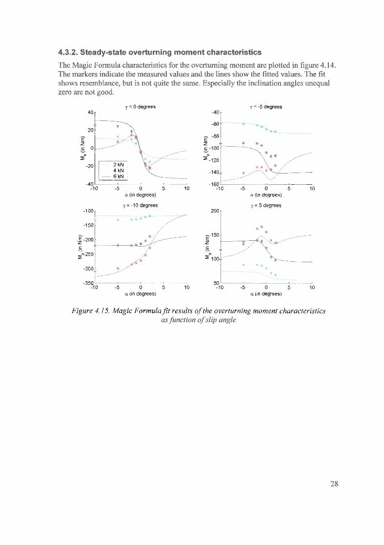
................................................................................................................... 4.2. Results -21 4.3. Magic Formula tyre model fit ................................................................................. 27

.................................................................................................................. 5 . Conclusions -29 ......................................................................................................... 6 . Recommendations 30

6.1. The research ............................................................................................................ 30 ............................................................................................... 6.2. Flat plank tyre tester 30

......................................................................................................................... References 32 ............................................................................................................................. Books 32 .......................................................................................................................... Articles -32

Course material .............................................................................................................. 32 A . Matlab files for the results ............................................................................................ 33

A.I. Loadflle.m .............................................................................................................. 33 .................................................................................................... A.2. L0adedRadius.m 33

.................................................................................. A.3. Conversion2AdaptedISO.m -33 A.4. 1nput.m ................................................................................................................... 34

...................................................................................................... A.5. C0mputedata.m 34 A.6. Fast.m ..................................................................................................................... 34

................................................................................................... A.7. FitStaticF0rces.m 35 ..................................................................................................... A . 8 . Measurement.m 36

A.9. PlotAl1.m ................................................................................................................ 37 .............................................................................................. A . 10 . Plot0verturning.m -37 ................................................................................................ A . 1 1 . P1otStaticforces.m 38

............................................................................................. A . 12 . P1otMeasurement.m 38 ................................................................................... B . Matlab structures for the results -39

......................................................................................................... B . 1 . Hub structure -39 ...................................................................................................... B . 2. Forces structure 39

........................................................................................................ B.3. Input structure 40

......................................................................... C . Matlab files for the Magic Formula fit 41 .................................................................................................... C . 1 . MagicFormulaFy 41

..................................................................................................................... C.2. FyObj 41

.................................................................................................................... C.3. FyCon -42 ................................................................................................. C.4. MagicFormulaMx -43

.................................................................................................................... C.5. MxObj 43 ...................................................................................................... C.6. LoadFittedData 44

................................................................................................... C.7. MagicFormulaFit A4 ........................................................................................................... C.8. PlotMagicFy 45 ......................................................................................................... C.9. PlotMagicMx 45

List of symbols

I Longitudinal force in the measuring hub I N K~ I Lateral force in the measuring hub

K7 1 Vertical force in the measuring hub

Tx I Longitudinal moment in the measuring hub

TY I Lateral moment in the measuring hub

T7 I Vertical moment in the measuring hub I Nm

FY I Lateral force in the contact point Fx

F, I Vertical load in the contact point I N

Longitudinal force in the contact point N

Mx

MY

M z

PP / Pneumatic scrub

a Y

Overturning moment in the contact point

Rolling resistance moment in the contact point

Self aligning moment in the contact point

Nominal load (Introduced to make parameters dimensionless in the Magic I

Nm

Nm

Nm

Slip angle Inclination angle

5

7,

rad rad

I moment I

Loaded radius (Length from the centre of wheel to the contact point)

Unloaded radius (Introduced to make parameters dimensionless in the Magic Formula model for overturning moment)

4sxx

h I Difference in height between centre of measuring hub and 1 m

m

m

Formula model for overturning moment) Parameter of the Magic Formula model for overturning -

h'

~ E T ( ET value of the wheel. I

a

arnh

track Difference in hei~ht between centre of wheel and track m Distance from centre of measuring hub to wheel centre Distance from centre of measuring hub to the rim

m m

1. Introduction More and more cars have a high centre of gravity, due to the growing market share of MPV's and SUV's. Roll-over is becoming a more important issue in vehicle dynamics. It is mostly dependent on the height of the centre of gravity. Conventional cars will slide before roll-over can occur. This is due to the low centre of gravity of these cars. Lateral accelerations needed to roll-over are not reached. Therefore roll-over accidents are mostly caused by tripping (A car rolls over due to an impact with an obstacle.). However SUV's and MPV's can come into a situation where lateral accelerations do get high enough to roll-over on even roads (without a tripping mechanism).

Real roll-over tests are precious, risky and hard to measure. That is why it is important to be able to simulate the behaviour precisely with a computer model. There are three important factors that determine the roll-over of a car:

Height of the centre of gravity: If the car is higher, the roll angles will be higher and the car rolls over quicker. Anti roll bar stiffness: If the car's roll stifhess is higher, the roll angles will be lower and the car rolls over less quickly. Overturning moment of the tyres: The forces and moments generated by the tyres contribute to the roll-over moment. Tvack width: If the car is smaller, the roll angles will be higher and the car rolls over quicker.

The subject of the traineeship will be: Is it possible to make a correct measurement of the overturning moment on the Flat plank tyre tester? Can the Magic Formula tyre model verzj?ed with these measurements? The model is based on measurements on the Flat track tyre tester and it is uncertain if the Magic Formula can still be used.

The report is divided in the following chapters:

First of all the overturning moment will be explained in chapter 2. This will include the definition and the characteristics. The Magic Formula model will also be given which is used for simulation models.

In chapter 3 the Flat plank tyre tester will be explained and how it will be used to meas-me the o v e ~ ~ r n g moment.

In chapter 4 the measurement data will be analysed and will be fitted with the Magic Formula model.

In chapter 5 some conclusions are drawn and in chapter 6 some recommendations are given.

2. Overturning moment 2.1. Definition

The overturning moment is the moment around the longitudinal axis of the wheel contact point. This cm be seec Ir? figme 2.1, ir, w h h d!!! forces, mme11ts m d mgks of the t y e are projected. These are all according to the adapted IS0 convention [ref. 81.

Z

Torque

Figure 2.1: Moments and forces [ . 31

The occurrence of the overturning moment is best explained with figure 2.2. When a tyre slips sideways, the tyre also tends to move sideways and the load distribution changes. The vertical load moves outside the contact point and a moment results: the overturning moment. Figure 2.2. shows that the overturning moment is the product of vertical load and pneumatic scrub. Both overturning moment and pneumatic scrub will have NEGATIVE sign when converted according to the adapted IS0 convention.

Figure 2.2: Overturning moment 1 6 3 1

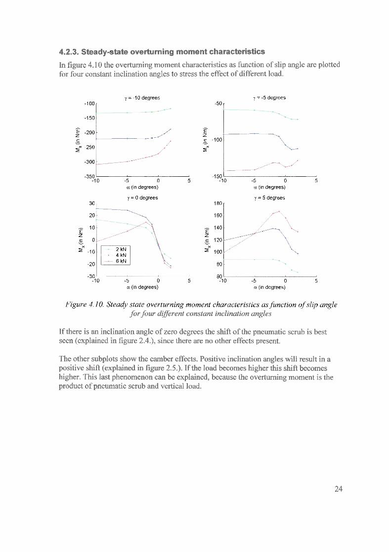
2.2. Characteristics In figure 2 straight (y

-3 the overturning moment characteristics are shown when the wheel = 0).

stands up

------- Figure 2.3. Overturning moment against slip angle

with constant inclination angle (y = 0) and various vertical loads [re$ I ]

It can be seen that the overturning moment switches sign when the vertical load changes. This is due to the fact that small vertical loads only use part of the tyre contact area. So the pneumatic scrub will be of opposite sign than the lateral force. The overturning moment will become negative. When the load increases the entire contact area is used. The pneumatic scrub gets the same sign as the lateral force and the overturning moment will become positive. This is shown in figure 2.4.

Figure 2.4. Overturning moment and vertical load dzflerence

The inclination angle changes have an important effect on the ovei-turning moment. Positive inclination angles shift the curves upward and negative inclination angles shift the curves downward. This shift in the curves is due to the shift of the contact point (C) which determines the pneumatic scrub (and thus the overturning moment). This phenomenon is explained in figure 2.5. The characteristics with inclination angle effects are shown in figure 2.6.

Figure 2.5. Overturning moment and inclination angle diference

Figure 2.6. Overturning moment against slip angle with various inclination angles and constant vertical load [veJ: I ]

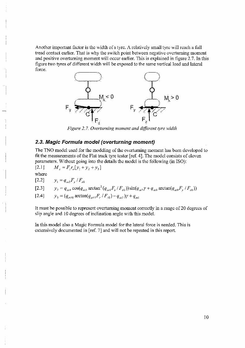
Another important factor is the width of a tyre. A relatively small tyre will reach a full tread contact earlier. That is why the switch point between negative overturning moment and positive overturning moment will occur earlier. This is explained in figure 2.7. In this figure two tyres of different width will be exposed to the same vertical load and lateral force.

f

Y 5 4

Figure 2.7. Overturning moment and dzferent tyre width

2.3. Magic Formula model (overturning moment)

The TNO model used for the modeling of the overturning moment has been developed to fit the measurements of the Flat track tyre tester [ref. 41. The model consists of eleven parameters. Without going into the details the model is the following (in ISO): P.11 M x = F z ~ , [ ~ , + ~ 2 + ~ 3 1 where

[2-21 Yl = q,,Fy K O

P.31 Y, = cos(qsx, arctm2 (q,,Fz 1 F z o )) sin(q,,y + q,, arctan(q,,Fy 1 S o ))

L2.41 Y3 = (4,10 arctan(q,ll< 4 0 ) - qsx2 )Y + 4,l

It must be possible to represent overturning moment correctly in a range of 20 degrees of slip angle and 10 degrees of inclination angle with this model.

In this model also a Magic Formula model for the lateral force is needed. This is extensively documented in [ref. 71 and will not be repeated in this report.

3. Measurements I Experiments 3. I. Flat plank tyre fester

The Flat plank tyre tester can be used to measure tyre behavior at a low speed. mxhine is shevm i~ f i p e 3.1.

-. F-F\

iciiuzrwr, gear be%.

:wsunng huh

I & I + ~ postton turn table adji*~t rnf:c:h.msn? " --7

I : ' 8-

The

Figure 3.1. Schematic view of the Flat plank tyre tester [re$ 61

A flat steel track moves horizontally. If this tracks rolls over the tyre forces and moments are generated in the wheel centre. These forces and moments are measured with the measuring hub and can be transformed to forces and moments in the contact point.

The following parameters can be adjusted, these include: Side slip angle

s inclination angle Constant vertical load or fixed axle height Track angle Track speed Braking

Instructions on how to operate the Flat plank tyre tester and a more detailed description can be fomd in the manual [ref. 51.

3.2. Transformafion of forces and momenfs

It is important to transform the measured values into forces and moments in the contact point. First the forces measured with the strain gauges need to be transformed into forces and moments in the centre of themeasuring hub. According to figure 3.2. these forces can be transformed as follows: (These are NOT the forces from Labview, but the forces converted in Adapted IS0 convention.)

Figure 3.2. Measuring hub [TI$ 61

[3.1] Kx=Gx1+Gx2

[3.2] Ky = Gy

[3.3] K, = G,, + G,, [3.4] Tx = ( a + b)G,, + bGZ2

[3.5] Ty = 0 ( 'Free rolling tyre' )

[3.6] TZ=(a+b)Gx,+bGx2

Now, according to figure 3.3, it is possible to transform the forces and moments in the measuring hub to the forces and moments in the contact centre:

Figure 3.3. The dzflerent axes

How to measure the loaded radius ( 5 ) correctly will be explained in the next section.

3.3. Measurement of loaded radius

The loaded radius is the most important variable in the computation of the overturning moment. Small changes in the loaded radius have a large effect on the overturning moment. This is due to the fact that the overturning moment is relatively small compared to the other moments and forces. An error of a mm can easily cause errors of 10 Nm in overturning moment. This will be explained with the following example. An error of a rnm in is an error of 3%0 in the loaded radius. The error in the product with the lateral load (of e.g. 3 kN) will then be 9 Nm. Off course, this will also be the error in the overturning moment.

The loaded radius can not be measured directly, instead the height between the wheel centre and the track and the inclination angle must be measured.

The adjustments in inclination angle can be achieved in two ways. The inclination angle itself can be adjusted and the track angle can be adjusted. Both methods have pros and cons and they are summed:

Inclination angle adjustment: It is difficult to adjust the inclination angle, because the procedure is difficult and it is difficult to get fhe angle right. The ET value (distance from wheel to wheel centre plane, see also in figure 3.5.) plays a role in determining the wheel centre and thus the loaded radius.

Track angle adjustment: Original vertical load need to be split in a vertical load on the track and an additional lateral force on the track.

0 Width cf the tyre plays importmt m!! h dctcmirAng the loaded rackis, beczise it detemlines where h e tyre contacts the track. The ET value plays a role in determining the wheel centre (and thus the loaded radius).

The inclination angle adjustment seems to be the best option, because it can be computed in the most direct way. According to figure 3.4. and 3.5. the loaded radius can be computed as follows:

gamma Figure 3.4. Loaded vadius

Figure 3.5. ET value and measuring hub [3.16] a = a,, -a,

The height between the wheel centre and the track could also be kept constant on the Flat plank tyre tester (instead of using a constant vertical load). This is not done, because one still has to calibrate the height correctly. If one measures height dynamically (e.g. with a LVDT) you aiso have to caiibrate the height once. The fixed axie height option only introduces a problem, because you no longer have a constant vertical load on the tyre.

3.4. Measurement accuracy

It is important to do the measurement with high accuracy. Small errors in particular quantities lead to severe errors in the overturning moment. Not only the loaded radius is important (as stated in the previous section). Static values of lateral force and the overturning moment in the wheel centre are important as well.

A static lateral force of 40 N may seem harmless (especially when the dynamic lateral force is in the order of thousands), but it will introduce a static overturning moment. The cause of this error could be an inaccuracy in the inclination angle and the track angle. A combined angle of 1 degree will result in a static lateral force which is approximately 2 % of the load Somewhat the same can be said about the overturning moment in the wheel centre. The inaccuracy of the inclination angle plays a role, it introduces an overturning moment (see section 2.2.). The distmce between the hub axle and the wheel centre can i~troduce a static overturning moment as well. An error of 1 mm will cause 2.5 Nm in the overturning moment.

3.5. Measurement procedure

The measurement procedure can be outlined in the following steps: The inclination angle and track angle need to be set to zero degrees. Therefore the static lateral force needs to be cancelled. The inclination angle can be measured precisely by turning the slip angle to 90 degrees. The track angle can no longer influence the static lateral force and the inclination angle can be adjusted. The static lateral force is purely due to the inclination angle. If the inclination angle is adjusted, it is possible to adjust the track angle. Off course this needs to be done with a slip angle of zero degrees on a non-moving track. If the static lateral force is close to zero, both inclination angle and track angle are set to zero. The angle between track and tyre is exactly 90 degrees. i%e height between the wheel centre and the track needs to be measuredprecisely. This needs to be done to be able to compute the loaded radius. It is measured by screwing a long bolt in the centre of the measuring hub and measure the distance till the track. Now the height can be measured with an accuracy of 0.5 mm, which is a reasonable accuracy. The distance between camber axis and the wheel centre needs to be 'measured '. (For simplicity the design sketches are used.) Adjust the inclination angle ifnecessary A digital clinometer can best be used for this purpose. Reset all channels when the tyve isfiee. All forces and the height variation are set to zero. The reference height is also set and can be read from the measuring rule on the back of the machine. (This reference height and the height variation has to be used to compute the loaded radius.) Start measurement.

4. Comparing and analysing the measurements In this chapter the measurement results are shown for a Continental tyre (205155 R16). In section 4.1. the raw data is shown. In section 4.2. the results are shown for lateral force, overturning moment and self aligning moment. The last section is used to fit lateral force and the o v e ~ ~ r m g moment with the use of the Magic %ornula.

4.1. Raw measurement data

In this section the raw data of the Flat plank tyre tester is shown. The data is computed and presented with Matlab. For now only a few measurements are shown. Measurements are done with different vertical loads (2, 4 and 6 kN), different slipangles (- 10, -5 , -2, - 1, 0, 1 and 2 degrees) and different inclination angles (-10, -5, 0 and 5 degrees). For now only a subset of the measurements is shown.

In figure 4.1. the moments and forces in the contact point (point C in figure 3.4.) are shown for a vertical load of 6 kN and an inclination angle of zero degrees. These moments and forces are plotted against travelled distance and with various slip angles.

The vertical load is kept constant pretty well with the use of the constant vertical load mechanism. Longitudinal force and rolling resistance moment are both negative, which indicates braking. The self aligning moment also behaves as expected. This corresponds with the literature (53 in ref 1 .). All plots show relaxation effects. After travelling a certain distance a steady state value is reached.

The lateral force for large slip angles is showing a strange dip at the end. It can be seen that this leads to a dip in the overturning moment as well. The lateral force with a slip angle of 10 degrees in the dip is the same as the lateral force with slip angle of 5 degrees in the top. When looking at the overturning moment the same can be said. This phenomenon will be explained in section 4.1.1.

Tnere is aiso a static overturning moment. This static value is assumed to be zero. Wnen the inclination angle is zero, the overturning moment needs to be zero when the tyre is not moving. These are errors in the setup of the Flat plank tyre tester and need to be compensated for. This is shown in section 4.1.2.

The lateral force also has a static value and is assumed to be zero. This can not be seen in figure 4.1, but it will be shown in 4.1.3.

Static measurement 8000:

Figure 4.5. Static measurement of overturning moment

4.4.3. Static lateral force

In the previous section the static overturning moment is explained. The same can be said about the static lateral force and the same measurement will show the static lateral force. This is shown in figure 4.6. The static lateral force will be used in the computed lateral force to compensate for the error in the setup.

Statrc measurement 8000 %

-1000 , 1 I -35 -30 -25 -20 -15 -10 -5 0 5

Fy jtn NN)

Figure 4.6. Static measurement of lateral force

The self aligning moment characteristics are shown in figure 4.9. The characteristics are as expected on the basis of the studied literature ($3 in ref 1 .).

-20 I -1 0 -5 0 5

a (in degrees)

-1 50 -1 0 -5 0 5

a (in degrees)

-100 -1 0 -5 0 5

a (in degrees)

y = -10 deg

--- y = 5 deg

Figure 4.9. Steady state self aligning moment characteristics ax function of slip angle for three vertical loads

5. Conclusions During this research experiments were done on the Flat plank tyre tester to measure the overturning moment generated by a tyre. These measurements are fitted with the Magic Formula tyre model to verify the model, which is based on measurements done on the Flat track tyre tester.

The conciusion of this research has to be that the Flat plank tyre tester is capable of doing fairly good overturning moment analysis. All possible causes for inaccuracies are minimized and that is why the inaccuracy in the overturning moment will be low enough.

The track angle and inclination angle can be set within tenths of degrees. This results in an error of 5 - 10 %, due to the higherllower lateral force. The static lateral force and static overturning moment are very close to zero. This results in a small absolute error (1 - 2 Nm). The loaded radius can be computed with an error of half a mm. This results in an error of 10 - 20 %.

All these inaccuracies combined will result in an error of approximately 10 % - 25 % in the overturning moment. At first this may seem a lot, but one has to keep in mind that the order of the overturning moment is a lot smaller than the vertical load (especially for inclination angles close to zero).

The Magic Formula fit for the overturning moment is not as good as expected. The shape of the fit is quite good, but it can not fit these data properly through the measured points. Especially the inclination angles unequal zero are not so good. This could be due to two reasons:

The tyre used now behaves different than the tyres which are used to model the Magic Formula. The Flat plank tyre tester gives different results than the Flat track tyre tester on which the Magic Formula is based. Flat track tyre tester uses a much higher speed and has a different setup. This can effect the overturning moment results.

6. Recommendations 6.1. The research

Because it was found that the measurement results could not be fitted accurately with the Magic Fomda, measwement results with the F!2t pplmuk tjre testa md the Flat trxk tyrs tester obtained under exactly the same conditions need to be compared. If the Flat track tyre tester gives different results with the same tyre under the saxe conditions, both machines need to be analysed thoroughly. The Magic Formula needs to be modified, if it appears that the Flat track tyre tester gives the same results, because it was found that the tyre behaves differently in comparison to the tyres used to develop the current Magic Formula model.

6.2. Flat plank tyre tester

In this section some recommendations are given to make the Flat plank tyre tester easier to work with.

Labview: The Labview model is not clear. It desperately needs to be rebuild. This need to be done by a programmer or a mechanical engineer with extended Labview experience. - The code must be structured in layers/subclasses. Only then the code is maintainable, readable and extendable. - The user interface must be split into a main menu and several separate windows. In the main menu it must be possible to open separate windows (some for input, output and options). - The axis system is not chosen properly [ref. 51. There are four conventions used in vehicle dynamics and the used axis system in Labview and in the manual is not one of them. In this report the adapted IS0 convention (Besselink) [ref. 81 is used. This could be used instead. - Initialisation is done several times in a loop and has to be done only once. Trigger: The trigger needs to be changed. It is better to use the rotational speed sensor of ihe plank to trigger a measurement (or trigger it manually). Track alignment: The Flat plank tyre tester shakes when the left side of the plank (front view) reaches the centre of the machine. There are also small vibrations in the measurements due to the track. Track alignment is already proposed in [ref. 61, but it is not possible to remove these vibrations. The only remedy: Do not use the constant height mechanism but use the constant force mechanism instead. Braking: The disk brake needs to be checked. If it can not be used properly, it needs to be replaced with some other braking mechanism. Motor control: The three rnotors (slip angle, track angle m-d track velocity) can be coupled with the computer. This makes the machine a lot more user friendly. Side slip angle: The side slip angle is measured with an encoder. This measures relative angles to the starting position. This starting point needs to be measured more precisely. Additional sensors: Some additional sensors are needed, which measure inclination angle and track angle.

e Wiring: The wiring needs to be checked and marked. There are loose connectors and unmarked wires. Constant force mechanisme: The operating device is at the front of the machine. This is not practical.

References Books

1. Pacejka, H.B., Tyre and vehicle dynamics, B.&te~worth-He?nernam (2002) ISBN 0 7506 5141 5

2. Beckwith, T.G.; Marangmi, R.3. Lienhard, J.H., Mechanical measurements, Addison-Wesley (1 995) ISBN 0 201 56947 7

Arficles

3. Takabashi, T.;Masatoshi, H., Modelling of Tire Overturning Moment Characteristics and the Analysis of n e i r Influence on Vehicle Rollover Behaviour, R&D Review of Toyota CRDL Vol. 38 No. 4 (2003)

4. Cortiana, G.; Oosten, J.J.M v., New Overturning Moment Model and Sensitivity Analysis of Roll-over Stability, TNO (2002)

5. Blom, R.E.A.;Vissers, J.P.M., Manual for the Flatplank tyre tester, TU/e (2003)

6. Blom, RE.A.;Vissers, J.P.M., Experiments on the Flat plank tyre tester, TU/e (2003)

7. Delft-Tyre, Using the MF-Tyre Model, TNO (2004)

Course material

8. Besselink, I.J.M., Vehicle Dynamics (Sheets), TU/e (2002-2003)

9. Rill, G., Vehice Dynamics (Lecture notes), Fachhochschule Regensburg (2003)

A. Matlab files for the results In this chapter the Matlab files will be shown for the processing of the results. In the next chapter the corresponding Matlab structures will be shown.

eval ( [ ' data=load ( ' ' '

%forces len = length (data ( : , 1 hub.forces.Kx = data( hub.forces.Ky = data( hub.forces.Kz = data(

ile ' ' ' ) ; ' I ) ;

hub.forces.Tx = data(:,4); hub.forces.Ty = zeros (1, len) ' ; hub.forces.Tz = -data(:,5);

%wheel parameters hub. wheel. angle = -data ( : ,9 ) ; %in Rad hub.wheel.velocity = data(:,8); %in Rad/s hub.wheel.slipangle = data(:,12); %in Degrees hub-wheel-dh = data(:,6) /1000; %Relative distance wheel centre to track

%in m %track parameters hub. track. displacement = -data ( : . 11) ; %in m hub.track.velocity = data(:, 10) ; %in m/s

% LoadedRadius % % Computation of the loaded radius

%Distance from turning point measuring hub to front of measuring hub a-mh = 0.3;

%Distance from turning point measuring hub to wheel centre a = a-mh + a - offset - a-et;

%Distance from wheel centre to track (lateral to track) hl = h + a*sin(gamma);

%Loaded radius (Distance from wheel centre to track in wheel plane) rl = hl/cos (gamma) ;

%moments conversion forces.Fx = hub.forces.Kx; forces.Fy = hub.forces.Ky*cos(gamma) + hub.forces.Kz*sin(gamma); forces.Fz = -hub.forces.Ky*sin(gamma) + hub.forces.Kz*cos(gamma);

%forces conversion forces.Mx = hub.forces.Tx - hub.forces.Ky.*rl; forces.My = hub.forces.Kx.*rl*cos(gamma) + hub.forces.Tz*sin(gamma); f0rces.M~ = -hub.forces.Kx.*rl*sin(gamma) + hub.forces.Tz*cos(gamma);

function input = Input (file) %----------------------------------------------------------

% Input %

% Check file, chop the data and put into an object % % Input: % - file: file (format ... \l.p .. a.h.g .-... ) % - defaultpath: path, which is added to file if neccessary P

% output % - input: object with all input parameters hidden in the filename , 1 -> load P p -> pressure % a -> slipangle , h -> reference height P g -> inclination angle (optional, default = 0) , - -> text for additional info (eg a number) %----------------------------------------------------------

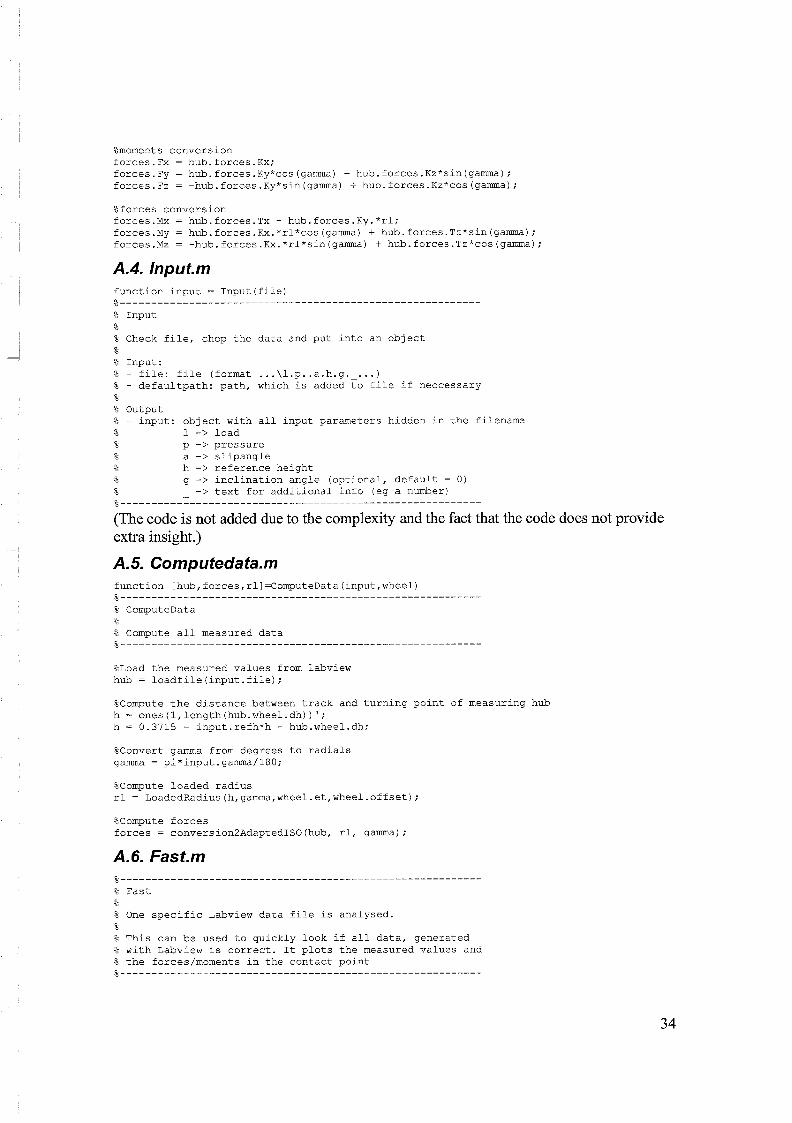
(The code is not added due to the complexity and the fact that the code does not provide extra insight.)

% ComputeData P

% Compute all measured data P----------------------------------------------------------

%Load the measured values from labview hub = loadfile (input. file) ;

%Compute the distance between track and turning point of measuring hub h = ones (1, length (hub. wheel. dh) ) ' ; h = 0.3715 - input.refh*h - hub.wheel.dh;

%Convert gamma from degrees to radials gamma = pi*input.gamma/l80;

%Compute loaded radius rl = LoadedRadius(h,gamma,wheel.et,wheel.offset);

%Compute forces forces = conversion2AdaptedISO(hub, rl, gamma);

clear all close all

%Default settings for used wheel wheel.et = 0.05; wheel.offset = 0.06;

defaultpath = 'e:\tue\stage\data\';

%Fetch the required parameters for the analysis file = input('Which file do you want to analyse? (Enter filename):','^');

%Fetch all data from the filename input = Input(file, defaultpath);

if input .valid input.gama = -input.gama;

%Compute all dara [hub, forces, rll = ComputeData (input,wheel) ;

%Plot all PlotAll (hub, forces, rl, 'k' )

else disp ('The file isn' 't valid' )

end

function staticforces = FitStaticForces(hub,forces,input) S - - - - - - - - - - - - - - - - - - - - - - - - - - - - - - - - - - - - - - - - - - - - - - - - - - - - - - - - - -

% FitStaticForces 9.

% All relevant static moments/forces are computed with a polynomial % fit of zero degree only in the constant part of the measurement. % These moments/forces are the overturning moment, self aligning moment % and lateral force. %----------------------------------------------------------

if input.angle < 2.5 %Long relaxation length disp begin = 1.2; %NO dip compensation disp-end = 0;

else %Short relaxation length disp-begin = 0.5; %Dip compensation disp-end = 1;

end

%Set the range tStart = 1; tEnd = length (forces .Mx) ; for i = 1:l:tEnd

if hub. track. displacement (i) > disp-begin %Starting point tStart = i; break

end end if disp-end == 1

for i = tStart:l:tEnd if hub.track.displacement(i) > disp-end

%Ending point tEnd = i; break

end end

end

%Find xf and yf for the fit for i = tStart:l:tEnd

xf(i - tStart + 1) = i - tStart + 1; Fy(i - tStart + 1) = forces.Fy(i); Mx(i - tStart + 1) = forces.Mx(i) ; Mz(i - tStart + 1) = forces.Mz(i);

end

%Fit the lateral force and overturning moment fitFy = polyfit (xf,Fy,O); fitMx = polyfit (xf ,Mx, 0) ; staticforces.Mz = polyfit (xf,Mz, 0) ;

%Correction by setting the static lateral force and overturning moment to zero %(See forcesweep file with camber zero for used values) switch input.load case 2000

staticforces.Fy = fitFy - 21; staticf0rces.M~ = fitMx + 1;

case 4000 staticf0rces.F~ = fitFy - 18; staticforces.Mx = fitMx - 7;

case 6000 staticforces.Fy = fitFy - 15; staticforces.Mx = fitMx - 13;

otherwise %No measurement done with this load staticforces.Fy = fitFy; staticforces.Mx = fitMx;

end

% Measurement P

% A set of Labview data file is analysed. s

% This file is used to compare several measurements with each % other. Mainly it is used comparing different slip angles at % constant load and constant inclination angle. % It plots several graphs and writes the relevant 'fitted' data % into a Matlab data file to use for further analysis. %----------------------------------------------------------

clear all close all

%Plot parameters files = {'12p25a2h5gO-top.fptt','12p25alh5gO_top.fptt', ... 1;

colors = {'b','rT,'k','r','b','m','g'};

defaultpath = 'e:\tue\stage\data\';

%Default settings for used wheel wheel.et = 0.05; wheel.offset = 0.06;

%Initialisation maxi = min(1ength (files) ,7) ;

for i = 1:l:maxi

file = files{i};

%Fetch all parameters from the filename input = Input (file, def aultpath) ;

if input .valid

end

%Display file parameters disp(' ' ) disp(['Computation for file: ' input.file]) disp(['Load: ' num2str(input.load/1000,2) ' kN'1) disp(['Tyre pressure: ' num2str(input.pressure,2) ' bar']) disp(['Slip angle: ' num2str(input.angle) ' degrees']) disp ( [ ' Inclination angle: ' nm2str (input. gamma) ' degrees' 1 )

%Compute all measured data [hub,forces,rl] = ComputeData(input,wheel);

%Plot all data PlotOverturning(hub,forces,rl,colors{i])

%Compute all static forces staticforces = FitStaticForces(hub,forces,input);

%Plot fitted data PlotStaticForces(hub,forces,input,staticforces,colors{i])

%Store all computed data eval ( eval ( eval ( eval ( eval ( eval ( eval ( eval (

hub',num2str (i) , '=hub; 'I) 'r11,num2str (i) , '=rl; ' 1 ) forces',num2str(i),'=forces;'l) 'input',nm2str (i) , '=input; 'I) fittedmx ( ' ,num2str (i) , ' ) =staticforces .Mx; ' I )

fittedfy ( ' ,num2str (i) , ' ) =staticforces .Fy; ' I ) fittedmz (',num2str(i), ')=staticforces.Mz; 'I) 'angles ( I , num2str (i) , ')=input .angle; 'I )

end

%Save all fitted data fz = inputl.load; eval(['save ..\data\l',num2str(inputl.load/1000),'g',num2str(inputl.gama),' fittedfy fittedmx fittedmz angles fz files'])

%Clear all local data clear hub rl forces input wheel maxi i file staticforces fz angles

% Pl0tAll P

% All pure data imported from labview is plotted in figure 11 and % figure 13 (resp. forces/moments and remaining data) from % one specific measurement. % All forces/moments in the contact point is plotted in figure 12 from % this specific measurement. % All forces/moments are in the adapted IS0 convention.

function [I = PlotOverturning (hub, forces, rl, color) %----------------------------------------------------------

% PlotStaticForces ,

% All relevant static moments/forces are plotted in figure 2 from % one specific measurement. % These moments/forces are the overturning moment, self aligning moment % and lateral force. %-- - - - - - - - - - - - - - - - - - - - - - - - - - - - - - - - - - - - - - - - - - - - - - - - - - - - - - - - -

% PlotMeasurement P

% All data from all measurements is plotted in six different % figures. % The first plot shows the lateral load. The next two plots show % the overturning moment. The fourth plot shows the self aligning % moment. The last two plots show the pneumatic scrub. %-- - - - - - - - - - - - - - - - - - - - - - - - - - - - - - - - - - - - - - - - - - - - - - - - - - - - - - - - -

B. Matlab structures for the results B. I . Hub structure

forces

wheel F

I 1 velocity

This stmctwe contains a!! Labview data cmverted ir, the adapted IS0 convention. This structure consists of the following fields "forces". "wheel" and "track". This structure contains all forces and moments in the measuring hub according to adapted ISO. This structure consists of the following fields "Kx", "Ky", "Kz", "Tx", "Ty" and "Tz". Longitudinal force in the measuring hub. Lateral force in the measuring hub. Vertical force in the measuring hub. Longitudinal moment in the measuring hub. Lateral moment in the measuring hub. Vertical moment in the measuring hub. This structure contains all wheel parameters. This structure consists of the following fields "angle", "velocity", "slipangle" and "dh". The rotational angle of the wheel. The rotational velocity of the wheel. The slip angle of the wheel The height difference from a certain reference point. This structure contains all track parameters. This structure consists of the following fields "forces", "wheel" and "track". The track displacement. The track velocity.

B.2. Forces structure

1 forces I This structure contains all forces and moments in the contact point I according to adapted ISO. This structure consists of the following fields "Fx", "Fy", "Fz", "Mx", "My" and "Mz".

1 Mz I Vertical moment in the contact point.

Fx FY Fz Mx Mu

Longitudinal force in the contact point. Lateral force in the contact point. Vertical force in the contact point. Longitudinal moment in the contact point. Lateral moment in the contact ~o in t .

5.3. Input structure

0 p + pressure in tenths of bars a + slip angle in degrees

input

Jile valid

h + reference height in cm g + inclination angle in degrees (optional, default is zero)

This structure contains all input parameters which are hidden in the filename. This structure consists of the following fields "file", "valid", "load", "pressure", "angle", "refh" and "gamma". Complete filename. Is the filename of the following form: 1 p a h-g-n-fptt

1 -+ load inkN

load pressure angle reJh amma g

n + number (optional) e .@tt + "flat plank tyre tester" file extension

Vertical load in N. Tyre pressure in Bar. Slip angle in degrees. Reference height in m. Inclination angle in degrees.

C. Matlab files for the Magic Formula fit In this chapter the Matlab files will be shown for the Magic Formula fit.

C. 1. Magic Formula Fy function Fy = MagicFormulaFy (x, alpha, gamma, Fz) ; 9----------------------------------------------------------

% MagicFormulaFy ,

% This is the function to compute the Fy component of the magic formula. % % Input: % - x: Magic Formula parameters s - alpha: slip angle % - gamma: inclination angle % - Fz: vertical load

global FzO

%Parameters of the Magic Formula pcyl = x(1) ; pdyl = x (2) ; pdy2 = x(3) ; pdy3 = x (4) ; peyl = x(5) ; pey2 = x (6) ; pey3 = x(7) ; pey4 = x(8) ; pkyl = x (9) ; pky2 = x (10) ; pky3 = ~ ( 1 1 ) ; phyl = ~ ( 1 2 ) ; phy2 = ~ ( 1 3 ) ; phy3 = x(l4) ; pvyl = ~ ( 1 5 ) ; pvy2 = x (16) ; pvy3 = ~ ( 1 7 ) ; pvy4 = ~ ( 1 8 ) ;

% Computation of the Fy component of the Magic Formula dFz = (Fz - FzO)/FzO; gammay = gamma;

shy = (phyl + phy2*dFz) + phy3*gammay; Svy = Fz * ((pvyl + pvy2*dFz) + (pvy3 + pvy4*dFz) * gammay ) ;

alphay = alpha + shy;

Ey = (peyl + pey2*dFz) * (1 - (pey3 + pey4*gammay) *sign(alphay) ) ; muy = (pdyl + pdy2"dFz) * (1 - pdy3*gammayA2);

Cy = pcyl; ~y = muy*Fz;

Fy = Dy * sin (Cy * atan (ByXalphay - Ey* (By*alphay - atan (By*alphay) ) ) ) + Svy;

C.2. FyObj function f = FyObj (x) ;

% for the Magic Formula fit (Fy component). % The objective function is based on a least square fit. %-- - - - - - - - - - - - - - - - - - - - - - - - - - - - - - - - - - - - - - - - - - - - - - - - - - - - - - - - -

global gamma Fz Fy alpha

f = 0; for i = 1 : 1 : length(Fy)

MFFY (i) = MagicFormulaFy (x, alpha (i) , gamma (i) , Fz (i) ) ; f = f + 100 * sqrt(((Fy(i) - MFFY(~))^~)/(FY(~)^~));

end f = f/length(Fy) ;

% Visualise how the fit is doing figure (11) plot (alpha,MFFY, 'r. ' ,alpha, Fy, 'ko') drawnow

C.3. FyCon function [g, geq] = FyCon(x) %--- - - - - - - - - - - - - - - - - - - - - - - - - - - - - - - - - - - - - - - - - - - - - - - - - - - - - - - -

% FyCon P

% This is the constraint function for Fy to compute the parameters % for the Magic Formula fit (Fy component). % This function computes inequality constraints and equality % constraints. %-- - - - - - - - - - - - - - - - - - - - - - - - - - - - - - - - - - - - - - - - - - - - - - - - - - - - - - - - -

global FzO global all-gammas all-loads

%Parameters of the Magic Formula pcyl = x(1) ; pdyl = x (2) ; pdy2 = x (3) ; pdy3 = x (4) ; peyl = x(5) ; pey2 = x(6); pey3 = x(7); pey4 = x(8) ; pkyl = x(9) ; pky2 = x(10) ; pky3 = ~ ( 1 1 ) ; phyl = x(12); phy2 = x(l3); phy3 = x(l4) ; pvyl = x (15) ; pvy2 = x(16) ; pvy3 = x(17); pvy4 = ~ ( 1 8 ) ;

%Inequality constraints (<= 0) i = 0; for il = 1 : length(al1-gammas)

for i2 = 1 :length(all-loads) i = i + l ;

dFz = (all-loads(i2)-FzO) / FzO; gammay = all-gammas (il) *pi/l8O;

Ey = (peyl + pey2*dFz) * (1 - (pey3 + pey4*gammay) ) ; g(2*i-1) = Ey - I;

Ey = (peyl + pey2*dFz) * (1 + (pey3 + pey4*gamrnay)); g(2*i) = Ey - 1;

end end

%Equality constraints (= 0) geq = 1 1 ;

C. 4. Magic Formula Mx Function Mx = MagicFormulaMx (x, alpha, gamma, Fz, Fy) ; %--- - - - - - - - - - - - - - - - - - - - - - - - - - - - - - - - - - - - - - - - - - - - - - - - - - - - - - - -

% MagicFormulaMx 3-

% This is the function to compute the Mx component of the Magic Formula. P

% Input: % - x: Magic Formula parameters % - alpha: slip angle % - gamma: inclination angle % - Fz: vertical load P - Fy: lateral force

global FzO RO

%parameters qsxl = x(1) ; qsx2 = x (2) ; qsx3 = x (3) ; qsx4 = x (4) ; qsx5 = x (5) ; qsx6 = x (6) ; qsx7 = x (7) ; qsx8 = x(8); qsx9 = x (9) ; qsxl0 = x (10) ; qsxll = x (11) ;

% Computation of the Mx component of the ~ a g i c Formula yl = qsx3 * Fy/FzO; y2 = qsx$ * cos (qsx5 * (atan(qsxG*Fz/FzO) ) "2) * sin(qsx7*gamma + qsx8*atan (qsxg*~y/FzO) ) ; y3 = (qsxlo * atan(qsxll*~z/~zO) - qsx2)*gamma + qsxl;

C.5. MxObj function f = MxObj (x) ;

global gamma Fz Fy Mx alpha global MFFyParams

f = 0; for i = 1 : 1 : length(Fy)

MFFy = ~agic~ormulaFy (MFFyParams, alpha (i) , gamma (i) , Fz (i) ) ; MFMX (i) = P!agicFormulaMx (x, alpha (i) , gamma (i) , Fz (i) , MFFy) ; f = f + 100 * sqrt(((Mx(i) - MF~~(i))"2)/(Mx(i)"2));

end

% Visualise how the fit is doing figure (12) plot (alpha,MFMX, 'r. ',alpha,Mx, 'ko') drawnow

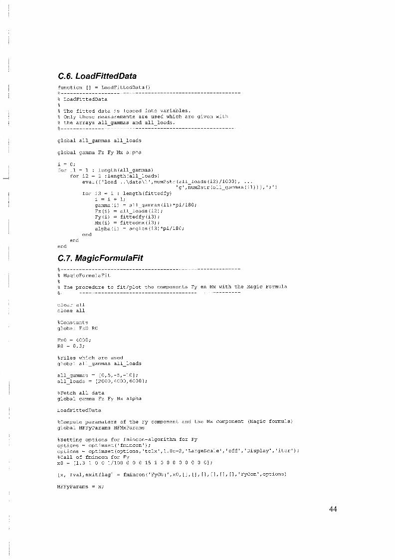
% LoadFittedData P

% The fitted data is loaded into variables. % Only those measurements are used which are given with % the arrays all - gammas and all-loads. %----------------------------------------------------------

global all-gammas all-loads

global gamma Fz Fy Mx alpha

i = 0; for il = 1 : length(al1-gammas)

for i2 = 1 :length(all-loads) eval(['load ..\data\l',num2str(all-loads(i2)/1000), . . .

'g',num2str(all-gammas(i1)) I , I ; ' )

for i3 = 1 : length(fittedfy) i = i + l ; gamma (i) = all-gammas (il) *pi/l8O; Fz (i) = all-loads (i2) ; Fy (i) = fittedfy (i3) ; Mx (i) = fittedmx (i3) ; alpha (i) = angles (i3) *pi/l8O;

end end

end

C. 7. MagicFormula Fit

clear all close all

%Constants global FzO RO

%Files which are used global all-gammas all-loads

all-gammas = [0,5,-5,-101; all-loads = [2000,4000,60001;

%Fetch all data global gamma Fz Fy Mx alpha

LoadFittedData

%Compute paramaters of the Fy component and the Mx component (Magic formula) global MFFyParams MFMxParams

%Setting options for fmincon-algorithm for Fy options = optimset('fmincon'); options = optimset(options,'to1x1,1.0e-2,'LargeSca1e','off','Disp1ay','iter'); %Call of fmincon for Fy x0 = [1.3 1 0 0 1/100 0 0 0 15 1 0 0 0 0 0 0 0 01;

[x, fva1,exitflagl = fmincon('FyObjt,xO, [I, [I, [I, [I, [I, [I, 'FyConl,options)

MFFyParams = x;

PlotMagicFy

%Setting options for fminunc-algorithm for Mx options = optimset('fminunc'); options = optimset(options,'tolx',l.0e-4,'LargeScale','off', ...

'HessUpdate','bfgsi, 'Display','itert); %Call of fmincon for Mx x 0 = [ 1 1 0 1 1 1 0 1 0 0 0 1 ;

[x, fval,exitflag] = fminunc ('MxObj ',xO,options) ;

MFMxParams = x;

PlotMagicMx

clear x xO fval exitflag options

C. 8. Plo tMagicFy

C. 9. PlotMagicMx