overlay networks formation: models and algorithms

POLITECNICO DI MILANODipartimento di Elettronica e Informazione

DOTTORATO DI RICERCA IN INGEGNERIA DELL’INFORMAZIONE

Overlay Networks Formation:Models and Algorithms

Doctoral Dissertation of:Jocelyne Elias

Advisor:Prof. Antonio Capone

Tutor:Prof. Michele D’Amico

Supervisor of the Doctoral Program:Prof. Patrizio Colaneri

2009-XXII

Abstract

Overlay networks have recently emerged as an effective means to provide a flexible,robust, and scalable platform for distributed applications, while leaving the underly-ing Internet infrastructure unchanged. This work tackles the overlay network designproblem considering both centralized and fully distributed approaches.

On one hand, we address the centralized overlay network design problem usingthe Service Overlay Network (SON) paradigm, and we propose several mathemat-ical models and heuristics for the optimal design of SONs. More specifically, weintroduce two network optimization models that determine the optimal assignmentof users to access overlay nodes, as well as the capacity reserved for each overlaylink, while taking accurate account of traffic routing. We also propose two overlaynetwork design models that further select the optimal number and location of theoverlay nodes to be deployed, as well as the optimal coverage of network users tomaximize the SON operator’s profit. Furthermore, we develop a set of efficient SONdesign heuristics to get near-optimal solutions for large-scale network instances in areasonable computation time. Finally, we perform an extensive performance evalua-tion of the proposed centralized optimization framework in several realistic networkscenarios.

On the other hand, this thesis also proposes two novel socially-aware overlaynetwork design games to deal with the fully distributed overlay network formationproblem. The first game combines both individual and social concerns in a unifiedand flexible manner, and the second game uses a Stackelberg approach, where theoverlay network administrator leads the users to a system-wide efficient equilibriumby buying an appropriate subset of the overlay network links. We evaluate the per-formance of the proposed games, through the determination of bounds on the Priceof Anarchy and other efficiency measures, as well as by simulating several realisticnetwork scenarios, including real ISP topologies.

Numerical results demonstrate that: (1) our proposed SON design models andheuristics plan very effective overlay networks, even in the case of very large net-work instances, and (2) our proposed distributed network formation algorithms areable to lead client users to form stable and efficient overlay networks, obtaining in

2

several cases the optimal solution that could be planned by a central authority. Hence,we conclude that the proposed solutions can be very effective when applied to realInternet scenarios.

3

Riassunto

Le reti overlay rappresentano una tecnologia efficace per fornire una piattaformaflessibile, robusta e scalabile per le applicazioni distribuite, mentenendo al contempointatta la struttura della rete Internet. La tesi di dottorato affronta il problema deldesign di reti overlay sia da un punto di vista centralizzato che totalmente distribuito.

Per prima cosa e stato affrontato il problema del design centralizzato di reti over-lay utilizzando il paradigma delle cosiddette Service Overlay Networks (SONs), pro-ponendo diversi modelli matematici ed euristiche per il progetto ottimale delle SON.Piu in dettaglio, sono stati introdotti due modelli di ottimizzazione che determinanol’assegnazione ottimale degli utenti ai nodi overlay di accesso, assieme al routing edalla capacita ottimale riservata su ogni link overlay.

Inoltre, sono stati proposti due modelli che selezionano anche il numero e la po-sizione ottimale dei nodi overlay da installare, cosı come la copertura piu efficientedegli utenti della rete al fine di massimizzare il profitto delloperatore di rete. Sonostate poi sviluppate delle euristiche efficienti per il design di reti SON, che ottengonorisultati vicini all’ottimo in breve tempo, anche per reti di grandi dimensioni. Infine,si e effettuata un’accurata valutazione delle prestazioni degli algoritmi e modelli pro-posti in diversi scenari di rete realistici.

Come ulteriore contributo, si sono proposti due nuovi giochi “socially-aware” peril design distribuito delle reti overlay, in particolare, e piu in generale per il problemadella formazione distribuita delle reti di telecomunicazione. Il primo gioco permettedi combinare sia interessi di tipo egoistico che sociale in modo unificato, mentre ilsecondo gioco utilizza un approccio alla Stackelberg nel quale l’amministratore dellarete stimola gli utenti a raggiungere un equilibrio di Nash globalmente efficiente,contribuendo alla formazione di un sottoinsieme appropriato dei link della rete over-lay. Si sono valutate le prestazione dei giochi proposti, determinando dei limiti al“price of anarchy” e ad altre misure di efficienza, simulando inoltre diversi scenaridi rete che includono anche topologie reali di Internet Service Provider. In sintesi, irisultati numerici hanno dimostrato che: (1) i modelli proposti per il design delle retiSON sono in grado di pianificare reti overlay molto efficienti, anche in presenza diistanze di rete molto grandi e (2) gli algoritmi distribuiti proposti per la formazione

4

delle reti conducono gli utenti a formare reti overlay stabili ed efficienti, ottenendonella maggior parte dei casi la soluzione ottimale che potrebbe essere progettata daun’autorit centrale.

List of Related Publications

1. J. ELIAS, F. Martignon, K. Avrachenkov, G. Neglia, Socially-Aware NetworkDesign Games, in Proceedings of the 29th IEEE Conference on ComputerCommunications (INFOCOM 2010), March 2010, San Diego, CA, USA.

2. E. Altman, J. ELIAS, F. Martignon, A Game Theoretic Framework for jointRouting and Pricing in Networks with Elastic Demands, in Proceedings ofthe Fourth International Conference on Performance Evaluation Methodolo-gies and Tools (VALUETOOLS 2009), October 2009, Pisa, Italy.

3. J. ELIAS, F. Martignon, G. Carello, Very Large-Scale Neighborhood SearchAlgorithms for the Design of Service Overlay Networks, submitted to Telecom-munication Systems, March 2009.

4. A. Capone, J. ELIAS, F. Martignon, Routing and Resource Optimization inService Overlay Networks, Elsevier Computer Networks, vol. 53, no. 2, 13February 2009, pp. 180-190.

5. A. Capone, J. ELIAS, F. Martignon, Models and Algorithms for the Design ofService Overlay Networks, IEEE Transactions on Network and Service Man-agement, vol. 5, no. 3, September 2008, pp. 143-156.

6. A. Capone, J. ELIAS, F. Martignon, Optimal Design of Service Overlay Net-works, in Proceedings of the Fourth International Telecommunication Net-working Workshop on QoS in Multiservice IP Networks, IT-NEWS 2008,Venice, Italy, February 2008.

Acknowledgements

I would like to thank my advisor, Professor Antonio Capone, for his support andguidance during my P.hD. studies at Dipartimento di Elettronica e Informazione,Politecnico di Milano. I will always appreciate his cheerful encouragement overthese three years.

I would also like to thank Professor Luigi Fratta and my tutor Michele D’Amicofor supporting me during my P.hD. studies.

I would like to express my sincere thanks to Professors Vicente Casares Ginerand Konstantin Avrachenkov for accepting to be my Thesis Reviewers.

I would like to thank Mr. Fabio Martignon for collaborating with me on severalvaluable ideas.

I am particularly grateful to Professors Philippe Nain, Eitan Altman, KonstantinAvrachenkov, Giovanni Neglia and all the MAESTRO team for my research visits atINRIA, Sophia Antipolis.

I wish to thank all my colleagues and friends at DEI, Politecnico di Milano.This thesis is dedicated to my family, to my parents on both sides and to all my

village.There is a long list of people to thank. All contributed in one way or another to

this thesis. To them all - I am forever thankful.

Table of contents

1 Introduction 11.1 Service Overlay Network Design . . . . . . . . . . . . . . . . . . . 21.2 Distributed Overlay Network Formation . . . . . . . . . . . . . . . 41.3 Thesis Contributions . . . . . . . . . . . . . . . . . . . . . . . . . 61.4 Thesis Structure . . . . . . . . . . . . . . . . . . . . . . . . . . . . 7

2 Related Work 92.1 Centralized Optimal Design of Service Overlay

Networks . . . . . . . . . . . . . . . . . . . . . . . . . . . . . . . 92.2 Distributed Overlay Network Design . . . . . . . . . . . . . . . . . 11

3 Service Overlay Networks Design: Models and Algorithms 133.1 User Assignment and Routing Models in Service Overlay Networks 14

3.1.1 Full Coverage User Assignment and Routing model . . . . . 163.1.2 Profit Maximization User Assignment and Routing Model . 18

3.2 Service Overlay Network Design Models . . . . . . . . . . . . . . 193.2.1 Full Coverage SON Design Model . . . . . . . . . . . . . . 203.2.2 Profit Maximization SON Design Model . . . . . . . . . . 21

3.3 Heuristics to Solve the SON Design Problems - Continuous relax-ation and randomized rounding based heuristics . . . . . . . . . . . 213.3.1 H-FCSD: a Heuristic to solve the Full Coverage SON

Design Problem . . . . . . . . . . . . . . . . . . . . . . . . 223.3.2 H-PMSD: a Heuristic to solve the Profit Maximization SON

Design Problem . . . . . . . . . . . . . . . . . . . . . . . . 26

4 Service Overlay Networks Design: Performance Evaluation 294.1 Random Topology Generators and Parameters

Setting . . . . . . . . . . . . . . . . . . . . . . . . . . . . . . . . . 304.2 User Assignment and Routing Models . . . . . . . . . . . . . . . . 31

i

4.3 Network Design Models and Heuristics . . . . . . . . . . . . . . . 37

5 Very Large-Scale Neighborhood Search Algorithms for the Design ofService Overlay Networks 565.1 User Assignment and Overlay Node Placement

Model . . . . . . . . . . . . . . . . . . . . . . . . . . . . . . . . . 575.2 Neighborhoods Definition . . . . . . . . . . . . . . . . . . . . . . 59

5.2.1 Polynomial Size Neighborhoods . . . . . . . . . . . . . . . 605.2.2 Very Large-Scale Neighborhood (VLSN) for the Allocation

Problem . . . . . . . . . . . . . . . . . . . . . . . . . . . . 615.3 TS-MCSD: a Very Large-Scale Neighborhood

Search Heuristic to Solve the MCSD Problem . . . . . . . . . . . . 645.3.1 Initial Solution . . . . . . . . . . . . . . . . . . . . . . . . 655.3.2 Iterative Very Large-Scale Tabu Search . . . . . . . . . . . 665.3.3 Post Optimization Step . . . . . . . . . . . . . . . . . . . . 69

5.4 Numerical Results . . . . . . . . . . . . . . . . . . . . . . . . . . . 69

6 Introduction to Game Theory 776.1 Strategic Games . . . . . . . . . . . . . . . . . . . . . . . . . . . . 776.2 Dominant Strategies . . . . . . . . . . . . . . . . . . . . . . . . . . 786.3 Nash Equilibrium . . . . . . . . . . . . . . . . . . . . . . . . . . . 796.4 Algorithmic Game Theory . . . . . . . . . . . . . . . . . . . . . . 80

6.4.1 Existence of Nash Equilibria . . . . . . . . . . . . . . . . . 816.4.2 Computing Nash Equilibria . . . . . . . . . . . . . . . . . 816.4.3 Bounding the prices of Anarchy and Stability . . . . . . . . 81

7 Socially-Aware Overlay Network Design Games 837.1 The Socially-Aware Network Design Game . . . . . . . . . . . . . 847.2 Best Response Algorithm . . . . . . . . . . . . . . . . . . . . . . . 867.3 Bounds on the Price of Anarchy, Price of Stability and Reachable

Price of Anarchy for the SAND game . . . . . . . . . . . . . . . . 877.4 The Network Administrator-Driven Socially-Aware Network Design

game . . . . . . . . . . . . . . . . . . . . . . . . . . . . . . . . . . 927.5 Numerical Results . . . . . . . . . . . . . . . . . . . . . . . . . . . 94

8 Conclusion 1008.1 Discussion and Concluding Remarks . . . . . . . . . . . . . . . . . 1008.2 Future Research Issues . . . . . . . . . . . . . . . . . . . . . . . . 101

References 102

ii

A Appendix A 111A.1 Overview of the Hub Location Problem . . . . . . . . . . . . . . . 111A.2 Overview of the Generalized Steiner and Steiner Tree Problems . . 112A.3 AMPL: A Modeling Language for Mathematical Programming . . . 113

List of Acronyms 114

List of Figures 115

List of Tables 118

iii

Chapter 1

Introduction

The Overlay Network paradigm has recently emerged as a viable and very effec-tive means to avoid network-level inefficiencies in the Internet, enabling, at the sametime, a variety of popular applications including peer-to-peer file sharing, contentdistribution and server deployment. Overlay Networks today represent an alterna-tive and very promising architecture able to provide end-to-end Quality of Serviceguarantees in the Internet, while leaving the underlying Internet infrastructure un-changed [1, 2, 3, 4].

Overlay networks are virtual topologies that use a combination of shared and ded-icated resources, to provide a simple network view that conceals unnecessary detailsabout the underlying topology. A typical overlay network architecture is depictedin Figure 1.1, where overlay nodes reside in the underlying ISP networks, and areinterconnected by virtual links which correspond to one or more IP-layer links.

Figure 1.1: Overlay Network Architecture.

1

The choice of where to install overlay nodes, which links establish between suchnodes and, in general, how to allocate resources to the overlay network has a deepimpact on the effectiveness of the resulting network and on its overall cost.

This thesis investigates two alternative approaches for the design of efficient over-lay networks, namely:

1. a centralized network optimization approach, which is based on the ServiceOverlay Network (SON) paradigm [1];

2. a fully distributed approach, where the overlay network design and operationis carried out by a large number of independent actors (e.g., the overlay userclients), all of whom seek to selfishly optimize their own utility.

In the remainder of this Chapter, we first illustrate the proposed centralized opti-mization approach for the overlay network design problem, introducing at the sametime the SON paradigm. Then, we focus on distributed overlay network manage-ment, proposing two novel overlay network formation games that lead user clients toform efficient overlay networks in a fully distributed, non-cooperative manner. Fi-nally, we summarize the main contributions and give the detailed structure of thisthesis.

1.1 Service Overlay Network Design

Service Overlay Networks (SONs) have recently emerged as alternative and verypromising architectures able to provide end-to-end Quality of Service guarantees inthe Internet, while leaving the underlying Internet infrastructure unchanged [1, 2, 3,4, 5].

A SON is an application-layer network built on top of traditional IP-layer net-works. In general, the SON is operated by a third-party ISP that owns a set ofoverlay nodes residing in the underlying ISP domains. These overlay nodes per-form service-specific data forwarding and control functions, and are interconnectedby virtual overlay links which correspond to one or more IP-layer links [1].

The service overlay architecture is based on business relationships between theSON, the underlying ISPs, and the users. The SON establishes bilateral service levelagreements with the individual underlying ISPs to install overlay nodes and purchasethe bandwidth needed for serving its users. On the other hand, the users subscribeto SON services, which will be guaranteed regardless of how many IP domains arecrossed by the users’ connection. The SON gains from users’ subscriptions. Al-though the quality requirements that a SON must satisfy may be different (e.g. band-width, delay, delay jitter, packet loss), we assume they are mapped to an equivalent

2

bandwidth [1, 5]. To assure the bandwidth for the SON, the underlying ISPs haveseveral technical options: they can lease a transmission line to the SON, use band-width reservation mechanisms or create a separate Label Switched Path if MPLS [6]is available in their networks.

Obviously, the deployment of Service Overlay Networks can be a capital-intensiveinvestment. It is therefore imperative to develop efficient network design tools thatconsider the cost recovery issue for a SON. The main costs of SON deployment in-clude the overlay nodes installation cost and the cost of the bandwidth that the SONmust purchase from the underlying network domains to support its services.

The topology design problem for Service Overlay Networks is considered by veryfew works [5, 7, 8, 9, 10, 11, 12, 13] which make several limiting assumptions:

• the number and location of overlay nodes are pre-determined, while the overlaynode placement is a critical issue in the deployment of the SON architecture.

• A full coverage of all traffic demands must be provided, while the main goalof a SON operator would be to maximize its profit by choosing which users toserve based on the expected revenue.

• The capacities of overlay nodes/links are unlimited, thus assuming that theunderlying ISPs will always be able to provide bandwidth to the SON.

• Only small network instances are considered, with a limited number of con-nections and overlay nodes.

This thesis overcomes these limitations by first addressing the joint user assign-ment and traffic routing problem, proposing two novel optimization models that de-termine the optimal assignment of users to access overlay nodes, as well as the ca-pacity reserved for each overlay link, while taking accurate account of traffic routing.The first model minimizes the network installation cost while providing full coverageto all the network’s users. The second model maximizes the SON profit by furtherselecting which users to serve in order to make its operation profitable, and also in-cludes a budget constraint that the SON operator can specify to limit its economicrisks in the deployment of the overlay network. We then extend such models to con-sider the more complex SON design problem, where the number and positions ofoverlay nodes to be deployed are optimized. To this end we present two SON designmodels that jointly optimize (1) the number and location of overlay nodes, (2) theuser assignment to access overlay nodes, (3) the traffic routing and (4) the capacitydimensioning of overlay links.

The SON design problems are NP-hard, however, the proposed Mixed IntegerLinear Programming (MILP) formulations can be solved to the optimum for realistic-size instances in reasonable time. More specifically, the formulation that considers

3

only the user assignment and routing problem can be solved to the optimum even forlarge-scale instances in a short computing time.

To tackle large-size instances for the global SON design problem, we propose twosimple but effective heuristic approaches able to provide near-optimal solutions in areasonable computation time. The proposed algorithms are based on the decomposi-tion of the model into sub-problems and on the solution of the continuous relaxation.0-1 feasible solutions are then obtained using a randomized rounding technique.

Regrettably, in some scenarios the proposed heuristics are unable to provide agood solution to the SON design problem due, in particular, to huge memory con-sumption and computational effort.

For this reason, we further propose an efficient tabu search based approach thatuses polynomial size and Very Large-Scale Neighborhoods (VLSN). VLSN is usedonce the local minimum is reached, to “escape” from it and widen the set of ex-plored solutions; it can therefore be seen as a diversification step for the tabu search.We demonstrate that the proposed VLSN-based heuristic is able to design efficientoverlay networks even in very large-scale topology scenarios.

1.2 Distributed Overlay Network Formation

In many scenarios, the overlay network design is not enforced by a central authority,but arises from the interactions of several self-interested agents: each user client candecide the set of connections to establish.

Network design with selfish users has been the focus of several recent works [14,15, 16, 17, 18, 19, 20], which have modeled how independent selfish agents canbuild or maintain a large network by paying for possible edges. Each user’s goal isto connect a given set of terminals with the minimum possible cost. Game theoryis the natural framework to address the interaction of such self-interested users (orplayers). A Nash Equilibrium (NE) is a set of users choices, such that none of themhas an incentive to deviate unilaterally. For this reason the corresponding networksare said to be stable.

However, Nash equilibria in network design games can be much more expensivethan the optimal, centralized solution. This is mainly due to the lack of cooperationamong network users, which leads to design costly networks.

Actually, the majority of existing works assume that users are completely non-cooperative. However, this assumption is not entirely realistic, for example whennetwork design involves long-term decisions (e.g., in the case of Autonomous Sys-tems peering relations). Moreover, incentives could be introduced by some externalauthority (e.g., the overlay administrator) in order to increase the users’ cooperation

4

level.In this work we overcome this limitation by first proposing a novel overlay net-

work design game, the Socially-Aware Network Design (SAND) game, where usersare characterized by an objective function that combines both individual and socialconcerns in a unified and flexible manner. More specifically, the cost function ofeach user is a combination of its own path cost (the selfish component) and the over-all network cost, which represents the social component. A parameter (α) weightsthe relative importance of the network cost with respect to the user path cost. Chang-ing the value of α permits to take into account different levels of social awareness oruser cooperation.

We investigate systematically the impact of cooperation among network agentson the system performance, through the determination of bounds on the Price ofAnarchy (PoA), the Price of Stability (PoS) and the Reachable Price of Anarchy(RPoA) of the proposed game. They all quantify the loss of efficiency as the ratiobetween the cost of a specific stable network and the cost of the optimal network,which could be designed by a central authority. In particular the PoA, first introducedin [21], considers the worst stable network (that with the highest cost), while thePoS [14] considers the best stable network (that with the lowest cost); finally, theRPoA considers only Nash equilibria reachable via best response dynamics fromthe empty solution [19]. Hence, PoA and RPoA indicate the maximum degradationdue to distributed users decisions (anarchy), while the PoS indicates the minimumcost to pay to have a solution robust to unilateral deviations.

Our analytical results show that as α increases, i.e., when users are more sensi-tive to the social cost, the PoS converges to 1, i.e., the best stable network is moreefficient, as expected. Surprisingly, an opposite result holds for the worst case. In-deed, for large α values (highly socially-aware users) the worst stable network canbe much more expensive than the networks designed by purely selfish users.

For this reason, we further propose a Stackelberg approach, the Network Ad-ministrator - Driven SAND game (NAD-SAND), which enables very efficient Nashequilibria, avoiding worst-case scenarios: a leader (e.g., the network administrator)buys an appropriate subset of the network links (i.e., those belonging to the min-imum cost generalized Steiner tree covering all source/destination pairs), inducingthe followers (the network users) to reach an efficient Nash equilibrium.

Summary of the main Numerical Results

We evaluate the performance of the proposed centralized and distributed overlaynetwork design approaches: first, we provide numerical results for the centralized

5

overlay network design approach in a set of realistic-size instances and investigatethe impact of different parameters on the SON design problem, such as number andinstallation cost of overlay nodes, bandwidth costs, traffic demands and SON oper-ator’s budget. We further determine bounds to the performance achievable by anyoptimization algorithm solving continuous relaxations of the proposed models. Thenumerical results show that in the considered network scenarios the proposed heuris-tics perform very close to the optimal solution provided by the integer models with ashort computing time.

Then, we measure the performance of the proposed distributed overlay networkformation games in several network topologies, including realistic scenarios whereplayers build an overlay on top of real Internet Service Provider networks, and weobserved that socially-aware users always generate better networks. Furthermore,we observe that the proposed Stackelberg approach achieves dramatic performanceimprovements in all the considered scenarios, even for small α values, since it leadsmost of the times to the optimal (least cost) network. Hence, introducing some in-centives to make users more socially-aware could be an effective solution to achievestable and efficient networks in a distributed way.

1.3 Thesis Contributions

In summary, the main contributions of this thesis are:

• two network optimization models that determine the optimal assignment ofusers to access overlay nodes, as well as the capacity reserved for each overlaylink, while taking accurate account of traffic routing.

• Two overlay network design models that further select the optimal number andlocation of the overlay nodes to be deployed, as well as the optimal coverageof network users to maximize the SON operator’s profit.

• A set of efficient SON design heuristics that get near-optimal solutions forlarge-scale instances in a reasonable computation time.

• An extensive performance evaluation of the proposed centralized optimizationframework in several realistic network scenarios.

• Two novel socially-aware overlay network design games: the Socially-AwareNetwork Design game, which combines both individual and social concernsin a unified and flexible manner, and a Stackelberg game where the overlaynetwork administrator leads the users to a system-wide efficient equilibriumby buying an appropriate subset of the overlay network links.

6

• A thorough numerical evaluation of the proposed games, through the deter-mination of bounds on the Price of Anarchy, the Price of Stability and theReachable Price of Anarchy of such games, as well as by simulation of severalrealistic network scenarios, including real ISP topologies.

1.4 Thesis Structure

The thesis is structured as follows:Chapter 2 discusses the most notable works related to the centralized overlay

design problem and to the distributed overlay network formation approach. Further-more, the novelties of the approaches proposed in this thesis are underlined comparedto existing network design schemes.

In Chapter 3, we first propose two novel user assignment and routing optimizationmodels, based on mathematical programming, which take into account the individualrequirements of the end-users, the connectivity between overlay nodes and the man-agement of traffic flows. The objective of the first model is the minimization of theoverall network installation cost while ensuring full coverage of all end-users. Thesecond model maximizes the SON profit by choosing which users to serve based onthe expected gain and budget constraints specified by the SON operator. We thenaddress the topology design problem for Service Overlay Networks, optimizing thenumber and positions of the overlay nodes to be deployed in addition to all the vari-ables considered in the user assignment and routing problem. Finally, we introducetwo efficient heuristics that obtain near-optimal solutions for large-scale instances ina reasonable computation time. Such heuristics are based on continuous relaxationand randomized rounding techniques.

Chapter 4 evaluates the performance of the models and heuristics introduced inthe previous Chapter in several realistic network scenarios.

In Chapter 5, we develop a novel and efficient heuristic approach that solvesthe user assignment and overlay node placement problem using tabu search alongwith polynomial size and very large-scale (VLSN) neighborhoods. VLSN is used toperform the diversification step on the local optimum obtained by tabu search. Wefinally provide numerical results of the proposed heuristic on a set of realistic, large-size instances, and discuss the effect of different parameters on the characteristics ofthe planned networks.

In Chapter 6, we give a short introduction to Game Theory, including strategicgames, dominant strategies, the Nash equilibrium concept and algorithmic game the-ory. An overview is provided on the existence and computation of Nash equilibria,as well as the definition of the price of anarchy and the price of stability performance

7

figures.In Chapter 7, we address the distributed overlay network formation problem us-

ing the game theory paradigm. To this aim, we first propose the Socially-AwareNetwork Design (SAND) game, where overlay clients are partially socially-awarebecause their utility function is a weighted sum of individual and global costs. Wealso study the efficiency of the equilibria achieved by our game, deriving boundsto the Price of Anarchy, the Price of Stability and the Reachable Price of Anarchy.Then, we introduce the Network Administrator-Driven SAND (NAD-SAND) gameusing a Stackelberg approach, where a leader (e.g., the overlay network administra-tor) architects the desired network buying an appropriate subset of network’s links,inducing the followers (the network users) to reach an efficient Nash equilibrium.The performance of the SAND and NAD-SAND games is measured in several net-work scenarios, including real ISP topologies, where players build an overlay on topof real Internet Service Provider networks.

Conclusions and directions for future work are presented in Chapter 8. Finally,Appendix A provides an overview of the Hub Location problem, the GeneralizedSteiner and Steiner Tree problems. A brief description of AMPL is also given.

8

Chapter 2

Related Work

This Chapter reviews the most notable works related to the centralized optimizationof overlay networks (Section 2.1) and to the distributed overlay network formationproblem (Section 2.2). In both cases, we point out the limitations of existing worksand the main novelties introduced in this thesis.

2.1 Centralized Optimal Design of Service OverlayNetworks

Several works have appeared in the literature with the purpose of providing optimalrouting and topology design in different contexts, such as wired backbone networks[22, 23, 24, 25], wireless networks [26, 27], and recently Service Overlay Networks[5, 7, 8, 9, 10, 11, 12, 13].

An adaptive topology design framework for SONs is presented in [5] to assureinter-domain QoS, and a set of heuristics is proposed to solve the least-cost topologydesign problem. A similar problem is investigated in [7], where end-systems andoverlay nodes are connected through ISPs that support bandwidth reservations; sim-ulated annealing is used as heuristic to provide solutions for large-sized networks.Another set of heuristics for SON design is proposed in [8]; these heuristics aim toconstruct an overlay topology maintaining the connectivity between overlay nodesunder various IP-layer path failure scenarios. However, all these works formulatethe design problem considering full coverage of all traffic demands and assumingthat locations of overlay nodes are given and the underlying ISPs are always able toprovide resources to the SON.

The work in [28] considers a generalized cost model in the formulation of thedesign problem, and provides both exact and approximate solutions.

9

A generalized framework for the SON design problem is proposed in [29] wheredifferent characteristics are considered: 1) single-homed/multi-homed end-systems2) usage-based/fixed cost model and 3) capacitated/uncapacitated networks. Optimaland approximation algorithms are also provided.

Reference [9] deals with dynamic topology construction to adapt to the underly-ing network topology changes. An architecture for topology-aware overlay networksis proposed to enhance the availability and performance of end-to-end applications byexploring the dependency between overlay paths. Several clustering-based heuristicsfor overlay node placement and a routing mechanism are also introduced.

The dynamic overlay network reconfiguration issue is addressed in [10], wherethe main goal is to find the optimal reconfiguration policies that can both accom-modate time-varying communication requirements and minimize the total overlaynetwork cost.

The problem of overlay node placement is addressed in [11, 12, 13]. In [11] theauthors consider how to place service nodes optimally in a network, balancing theneed to minimize the number of nodes and to limit the distance between users andservice nodes. This work, however, only proposes optimization algorithms for theuncapacitated version of the coverage problem. The work in [12] focuses on design-ing an overlay network that maximizes the number of unicast and multicast connec-tions with deterministic delay requirements, without considering link costs. Finally,the overlay node placement problem is investigated in [13] to improve routing reli-ability and TCP performance. This paper, however, assumes that overlay nodes andlinks have infinite capacities, and does not take into account the costs involved in thedeployment of the overlay network.

The construction of efficient multicast trees in overlay networks is the primaryfocus of several studies [30, 31, 32, 33], and is not considered in this thesis since wefocus our analysis on unicast traffic.

In summary, the above cited techniques are less general than our current worksince they deal with the design problem considering at least one of the followingspecial cases: 1) the number and location of overlay nodes are pre-determined,2) the routing is fixed and known, 3) there are no capacity constraints on overlaylinks/nodes, 4) full coverage of all network users is provided without consideringthe SON profit maximization issue, and 5) only small and medium-size topologiesare considered, with a limited number of connections and overlay nodes. Our worktackles the SON design problem taking into account all these issues within a generaloptimization framework that in addition considers the expected profit of the SONoperator and a budget constraint that can limit the economic risk. Furthermore, weunderline that none of the above works uses VLSN search techniques to solve theSON design problem. A survey on such techniques can be found in [34, 35].

10

2.2 Distributed Overlay Network Design

Several recent works focused on network design with selfish users [14, 15, 16, 17,18, 19].

The so-called Shapley network design game is proposed in [14]. In this game,each player chooses a path from its source to its destination, and the overall networkcost is shared among the players in the following way: each player pays for eachedge a proportional share of the edge cost, i.e., the edge cost divided by the numberof players that pass through such edge.

Of all the ways to share the social cost among the players, this proportionalsharing method enjoys several desirable properties. First, it is budget balanced, inthat it partitions the social cost among the players. Second, it can be derived fromthe Shapley value, and as a consequence is the unique cost-sharing method satisfy-ing certain fairness axioms. Third, it admits pure strategy NEs. Specifically, An-shelevich et al. showed in [14] that a pure-strategy Nash equilibrium always ex-ists, that PoA = k and the Price of Stability is equal to the k-th harmonic number,i.e. PoS = Hk =

∑ki=1 1/i = O(ln(k)).

The network design model presented in [15] by Anshelevich et al. is general anddoes not admit pure Nash equilibria, even for very simple network instances. Briefly,in such model each player i has a set of terminal nodes that he must connect. Astrategy of a player is a payment function pi, where pi(e) is how much player i isoffering to contribute to the cost of edge e. Any edge e such that

∑i pi(e) ≥ c(e)

is considered bought (c(e) being the link cost), and Gp denotes the graph of boughtedges with the players offering payments p = (p1, ..., pk). Since each player mustconnect its terminals, all of the player’s terminals must be connected in Gp. However,each player i tries to minimize its total payments,

∑e∈E pi(e).

The authors in [16] have extended the network design model in [14], includingweighted players: if wi denotes the weight of player i, then i’s cost share of an edge eis ce ·wi/We, where We is the total weight of the players that use a path containing theedge e. But while easy to define, this weighted network design game is challengingto analyze. In particular, it is shown in [16] that:

• Pure-strategy Nash equilibria exist in all weighted Shapley network designgames with two players.

• There are no larger classes of weighted Shapley network design games thatalways possess pure-strategy Nash equilibria. For example, it is illustrated a3-player game that does not possess a Nash equilibrium.

The works in [17, 18] study the existence of strong Nash equilibria (i.e., equilib-ria where no coalition can improve the cost of each of its members) in network design

11

games under different cost sharing mechanisms. Strong Nash equilibria ensure sta-bility against deviations by every conceivable coalition of agents. More specifically,the authors in [17] show that there are graphs that do not admit strong Nash equilib-ria, and then give sufficient conditions on the existence of approximate strong Nashequilibria.

Furthermore, the problem of designing a protocol that optimizes the equilibriumbehavior of the induced network game is investigated in [19]. The authors study thedesign of optimal cost-sharing protocols for undirected and directed graphs, single-sink and multicommodity networks, different classes of cost-sharing methods, anddifferent measures of the inefficiency of equilibria. Moreover, they provide upperand lower bounds on the best possible performance of non-uniform cost-sharing pro-tocols.

Few works have considered individual and social concerns of user agents whiledealing with different types of networking problems [36, 37].

A proposition that takes into account individual and social benefits has been con-sidered in [36] in the general context of multi-agent systems, where individual andsocial concerns can conflict, leading to inefficient system performance. To addresssuch problem, the authors have proposed a formal decision making framework, basedon social welfare functions, that combines both social and individual perspectives.

An experimental investigation of the impact of cooperation in the context of rout-ing games is conducted in [37]. The game is studied considering particular networktopologies (i.e., parallel links and load balancing networks), shared by several users.Each user seeks to optimize either its own performance or some combination be-tween its own performance and that of other users, by controlling the routing of itsgiven flow demand.

However, unlike our work, none of the above papers applies these concepts tothe network design game, nor provides a theoretical analysis of the efficiency of theachieved Nash equilibria.

12

Chapter 3

Service Overlay Networks Design:Models and Algorithms

Service Overlay Networks (SONs) create a virtual topology on top of the Internet,thus providing a valuable platform able to guarantee end-to-end quality of servicewithout requiring support by the underlying network.

The optimization of the resources utilized by a SON is a fundamental issue foran overlay operator owing to the costs involved and the need to satisfy user require-ments. Careful decisions are necessary to provide enough capacity to overlay links,to route traffic, to assign users to access nodes and to deploy overlay nodes.

This Chapter takes into account all these issues, proposing two mathematical pro-gramming models for the user assignment problem, the traffic routing optimizationand the dimensioning of the capacity reserved on overlay links in SONs. The firstmodel minimizes the SON installation cost while providing full access to all users.The second model maximizes the SON profit by selecting which users to serve, basedon the expected gain, and taking into consideration budget constraints of the SONoperator. Furthermore, we extend these models to include the optimization of thenumber and position of overlay nodes. Finally, we introduce two efficient heuristicsto get near-optimal solutions for large-scale instances in a reasonable computationtime.

The Chapter is structured as follows: Section 3.1 describes the proposed userassignment and traffic routing models, while Section 3.2 introduces the SON designformulations. Finally, Section 3.3 illustrates the proposed heuristics to plan large-scale overlay networks.

13

3.1 User Assignment and Routing Models in ServiceOverlay Networks

Table 3.1: Basic Notation for the SON design problem.I Set of Test Points (TPs)D Set of Destination Nodes (DNs)R Set of Overlay Nodes installed in the SONcBjl Cost for buying one bandwidth unit between CSs j and l

cAij Access cost per bandwidth unit between TP i and CS j

cEjk Egress cost per bandwidth unit between CS j and DN k

dik Traffic generated by TP i towards DN k

ujl Maximum capacity that can be reserved on overlay link (j, l)vj Maximum capacity of the access link of CS j

hjk Maximum capacity that can be reserved on egress link (j, k)aij 0-1 parameter that indicates if TP i can access the SON through CS j

ejk 0-1 parameter that indicates if CS j can be connected to DN k

bjl 0-1 parameter that indicates if CSs j and l can be connected with an overlay linkgi Revenue per bandwidth unit obtained for serving TP i

B SON operator’s budgetS Set of Candidate Sites (CSs)cIj Cost for installing an overlay node in CS j

xij 0-1 variable that indicates if TP i is assigned to CS j

wjk 0-1 variable that indicates if CS j is connected to DN k

yjl 0-1 variable that indicates if there is an overlay link between nodes j and k

fkjl Flow variable which denotes the traffic flow routed on link (j, l) destined to DN k

fjk Flow variable which denotes the traffic flow routed on egress link (j, k)zj 0-1 variable that indicates if an overlay node is installed in CS j

A common approach to the user assignment and routing problem is to considerfeasible positions of traffic concentration points in the service area (Test Points, TPs),which generate traffic towards one or more Destination Nodes (DNs) [22]; the place-ment of TPs and DNs depends on the expected traffic distribution. Although theconcept of test point is distinguished from end-user (formally, the end-user is thetraffic generation agent that is placed in a TP), we will use the two terms as syn-onyms throughout the thesis. Destination nodes can represent either terminal nodesor access points to other networks.

14

Let I = 1, . . . , n denote the set of TPs, D = 1, . . . , p the set of destinations andR = 1, . . . , r the set of overlay nodes installed in the SON. The basic notation usedin this Chapter is presented in Table 3.1.

The cost for the SON operator to buy one bandwidth unit between overlay nodes jand l from the underlying ISPs is denoted by cB

jl, while cAij is the access cost per

bandwidth unit required between TP i and node j. Finally, cEjk represents the cost

per bandwidth unit for the traffic transmitted on the egress link between node j anddestination node k ∈ D.

The traffic generated by TP i towards destination node k is given by the parameterdik, i ∈ I, k ∈ D. The maximum capacity that can be reserved by the SON operatorbetween nodes j and l on the overlay link (j, l) is denoted by ujl, j, l ∈ R, while themaximum capacity of the access link of node j is denoted by vj , j ∈ R.

According to TPs, DNs and overlay nodes’ geographic location and the underly-ing physical topology, the following connectivity parameters can be calculated.

Let aij, i ∈ I, j ∈ R be the test point coverage parameters:

aij =

⎧⎨⎩

1 if TP i can access the SON throughoverlay node j

0 otherwise

Similarly, let ejk, j ∈ R, k ∈ D denote destination nodes coverage parameters:

ejk =

⎧⎨⎩

1 if overlay node j can be connectedwith destination node k

0 otherwise

Obviously, aij depends on the proximity of TP i to node j, that is on the accesscoverage provided by the SON operator with node j through agreements with localnetwork operators. Similarly, ejk is related to the distance between DN k and node j.

Let bjl, j, l ∈ R denote the connectivity parameters between two different over-lay nodes, which may depend on the proximity of the overlay nodes j and l in theunderlay network, as well as on the agreements between the SON and the differentISPs.

bjl =

⎧⎨⎩

1 if nodes j and l can be connectedwith an overlay link

0 otherwise

Decision variables of the problem include TP assignment variables xij , i ∈ I ,j ∈ R:

15

xij =

{1 if TP i is assigned to overlay node j0 otherwise

destination assignment variables wjk, j ∈ R, k ∈ D:

wjk =

{1 if node j is connected to destination node k0 otherwise

connection variables yjl, j, l ∈ R:

yjl =

{1 if there is an overlay link between nodes j and l0 otherwise

and finally flow variables f kjl which denote the traffic flow routed on link (j, l) des-

tined for destination node k ∈ D. The special variables fjk denote the traffic flow onthe egress link between node j and destination node k.

Given the above parameters and variables, we propose two different user assign-ment and routing formulations. The first, called Full Coverage User Assignment andRouting model (FC-UAR), optimizes the user assignment and traffic routing mini-mizing the total network cost while ensuring full coverage of all end-users. The sec-ond formulation, called Profit Maximization User Assignment and Routing model(PM-UAR), maximizes the total network profit, choosing which users to serve basedon the revenue generated by their subscription to the SON services and the cost nec-essary to cover them.

3.1.1 Full Coverage User Assignment and Routing model

The Full Coverage User Assignment and Routing model (FC-UAR) optimizes theusers’ assignment and traffic routing minimizing the total network cost while ensur-ing full coverage of all end-users.

Minimize

{ ∑j,l∈R

∑k∈D

cBjlf

kjl +

+∑

i∈I,j∈R,k∈D

cAijdikxij +

∑j∈R,k∈D

cEjkfjk

}(3.1)

s.t.

16

∑j∈R

xij = 1, ∀i ∈ I (3.2)

xij ≤ aij , ∀i ∈ I, j ∈ R (3.3)

∑i∈I

dikxij +∑l∈R

(fklj − fk

jl) − fjk = 0, ∀j ∈ R, k ∈ D (3.4)

∑k∈D

fkjl ≤ ujlyjl, ∀j, l ∈ R (3.5)

∑i∈I,k∈D

dikxij ≤ vj, ∀j ∈ R (3.6)

fjk ≤ hjkwjk, ∀j ∈ R, k ∈ D (3.7)

yjl ≤ bjl, ∀j, l ∈ R (3.8)

wjk ≤ ejk, ∀j ∈ R, k ∈ D (3.9)

xij , wjk, yjl ∈ {0, 1}, ∀i ∈ I, j, l ∈ R, k ∈ D (3.10)

The objective function (3.1) accounts for the Service Overlay Network cost, in-cluding the costs related to the connection of overlay nodes, users’ access and egresscosts.

Constraints (3.2) provide full coverage of all TPs, while constraints (3.3) arecoherence constraints ensuring that TP i can be assigned to overlay node j only if ican be connected to j.

Constraints (3.4) define the flow balance in node j for all the traffic destined fornode k. These constraints are the same as those adopted for classical multicommodityflow problems. The term

∑i∈I dikxij is the total traffic generated by the assigned

TPs destined for destination node k,∑

l∈R fklj is the total traffic received by j from

neighboring nodes,∑

l∈R fkjl is the total traffic transmitted by j to neighboring nodes,

and fjk is the traffic transmitted towards the destination node k.Constraints (3.5) impose that the total flow on the link between overlay nodes j

and l does not exceed the capacity of the link itself (ujl). Constraints (3.6) imposefor each overlay node that the ingress traffic serviced by such network device doesnot exceed the capacity of the link used for the access, whilst constraints (3.7) force

17

the flow between node j and the destination node k to zero if node j is not connectedto k, and impose that such flow does not exceed the maximum capacity (hjk) of theegress link between overlay node j and destination node k.

Constraints (3.8) define the existence of an overlay link between nodes j and l,depending on the connectivity parameters bjl. Constraints (3.9) are coherence con-straints ensuring that a node j can be connected to a destination node k only if kis located in the proximity of node j. Finally, constraints (3.10) are the integralityconstraints for the binary decision variables.

It is easy to see that this problem is equivalent to the integer multi-commodityflow problem and therefore is NP-hard [38]. We show in Chapter 4, however, thatthis problem can be solved to the optimum even for large-size instances with a shortcomputing time.

Note that we can consider alternative formulations to the FC-UAR model. Forexample, we might want end-users to be connected to more than one overlay node,for redundancy. This is easily accomplished by modifying constraints (3.2) as:∑

j∈R

xij = η, ∀i ∈ I (3.11)

where η is the number of overlay nodes per end-user.

3.1.2 Profit Maximization User Assignment and Routing Model

The Profit Maximization User Assignment and Routing model (PM-UAR) maxi-mizes the SON operator’s profit, choosing which users to serve based on the revenuegenerated by their subscription to the SON services and the required cost to the SONprovider for covering them.

The objective function (3.1) is therefore changed as follows:

Maximize∑

i∈I,j∈R,k∈D

gidikxij −{ ∑

j,l∈R

∑k∈D

cBjlf

kjl

+∑

i∈I,j∈R,k∈D

cAijdikxij +

∑j∈R,k∈D

cEjkfjk

}(3.12)

where gi, ∀i ∈ I , represents the revenue per bandwidth unit that the SON operatorobtains covering Test Point i. Here we assume for simplicity that the price paid bythe i− th user is proportional to the amount of traffic the user introduces in the SON,∑

k∈D dik, with gi being the proportionality coefficient, but some general pricingmodels can be easily accounted for.

18

Constraints (3.2) are changed as follows, while all the other constraints are thesame as in the FC-UAR model: ∑

j∈R

xij ≤ 1, ∀i ∈ I (3.13)

With such formulation, the SON operator maximizes the network profit, obtainedby subtracting the total revenue, achieved by covering a subset of the Test Points, tothe cost necessary to deploy an overlay network satisfying the users’ requirements.Note that, differently from constraints (3.2) in the FC-UAR model, in this formula-tion constraints (3.13) do not impose full coverage of all TPs.

The Service Overlay Network designer may be required to stay within a givencost budget (B) to limit the economic risks in the deployment of the network. ThePM-UAR formulation can be modified to account for budget limitation simply by theaddition of the following constraint:∑

j,l∈R

∑k∈D

cBjlf

kjl +

∑i∈I,j∈R,k∈D

cAijdikxij +

∑j∈R,k∈D

cEjkfjk ≤ B (3.14)

3.2 Service Overlay Network Design Models

In this Section, we extend the models presented in Section 3.1, proposing two novelService Overlay Network design formulations, namely Full Coverage SON Designand Profit Maximization SON Design models, which also optimize the number andlocation of overlay nodes to be deployed.

To this end, in addition to Test Points and Destination Nodes, we consider fea-sible positions, called Candidate Sites (CSs), where overlay nodes can be installed[22]. The placement of CSs depends on the underlying network topology and theagreements of the SON operator with ISPs. Let S = 1, . . . , m denote the set of CSs,and cI

j the cost associated with installing an overlay node at CS j.Decision variables now include overlay node installation variables zj , j ∈ S:

zj =

{1 if an overlay node is installed in CS j0 otherwise

All the other variables and parameters are the same as defined in Section 3.1,where the overlay nodes set R is now replaced by the set of Candidate Sites, S.

19

3.2.1 Full Coverage SON Design Model

The Full Coverage SON Design model (FCSD), whose formulation is reported be-low, optimizes the number and location of overlay nodes minimizing at the same timethe total network cost and ensuring full coverage of all SON users.

The objective function can be obtained from (3.1) including the overlay nodesinstallation costs:

Minimize

{∑j∈S

cIjzj +

∑j,l∈S

∑k∈D

cBjlf

kjl +

+∑

i∈I,j∈S,k∈D

cAijdikxij +

∑j∈S,k∈D

cEjkfjk

}(3.15)

The problem variables are subject to constraints (3.2), (3.4)-(3.8) and to the fol-lowing constraints.

TP i can be assigned to CS j only if an overlay node is installed in j and if i canbe connected to j:

xij ≤ zjaij , ∀i ∈ I, j ∈ S (3.16)

The existence of an overlay link between CSs j and l depends on the installationof nodes in j and l, and is defined by:

yjl ≤ zj, yjl ≤ zl, ∀j, l ∈ S (3.17)

Coherence constraints ensure that a CS j can be connected to a destination nodek only if an overlay node is installed in j and if k can be connected to j:

wjk ≤ ejkzj , ∀j ∈ S, k ∈ D (3.18)

Finally, the integrality constraints for the binary decision variables are:

xij , zj , wjk, yjl ∈ {0, 1}, ∀i ∈ I, j, l ∈ S, k ∈ D (3.19)

The FCSD problem is therefore defined by the objective function (3.15) subjectto constraints (3.2), (3.4)-(3.8) and (3.16)-(3.19).

20

3.2.2 Profit Maximization SON Design Model

The Profit Maximization SON Design model (PMSD) maximizes the SON operator’sprofit, selecting the optimal number and location of overlay nodes to be deployed,and choosing which users to serve based on the expected gain and the cost necessaryto satisfy their traffic demands.

The PMSD formulation is obtained by modifying the objective function (3.15) asfollows:

Maximize∑

i∈I,j∈S,k∈D

gidikxij −{∑

j∈S

cIjzj +

+∑j,l∈S

∑k∈D

cBjlf

kjl +

∑i∈I,j∈S,k∈D

cAijdikxij +

∑j∈S,k∈D

cEjkfjk

}(3.20)

and by introducing constraints (3.21), as for the PM-UAR model:∑j∈S

xij ≤ 1, ∀i ∈ I (3.21)

All other constraints are the same as in the FCSD model.Finally, a cost budget can be introduced in PMSD simply by adding the following

constraint:

∑j∈S

cIjzj +

∑j,l∈S

∑k∈D

cBjlf

kjl +

+∑

i∈I,j∈S,k∈D

cAijdikxij +

∑j∈S,k∈D

cEjkfjk ≤ B (3.22)

3.3 Heuristics to Solve the SON Design Problems -Continuous relaxation and randomized roundingbased heuristics

The computing time required to obtain an optimal solution for both the FCSD andPMSD problems might be very long for medium-to-large-size instances. As an ex-ample, the average computing time required to solve at optimum random network in-stances with the FCSD model grows exponentially from 10 s for CS=30 up to 4600 sfor CS=50, when run on an Intel Pentium 4 (TM) processor with CPUs operating at

21

3 GHz and with 1024 Mbyte of RAM, which is the workstation used to obtain thenumerical results reported in the next Chapter. For this reason, we propose hereaftertwo simple but effective heuristics, named H-FCSD and H-PMSD, that provide near-optimal solutions in a reasonable amount of time for the Full Coverage and the ProfitMaximization SON Design problems, respectively.

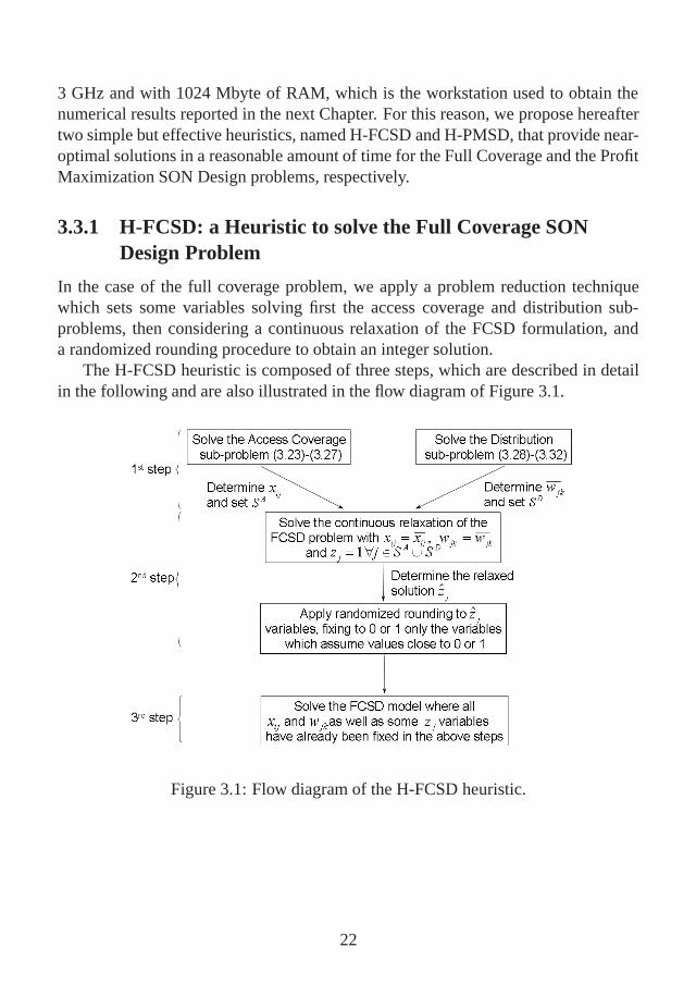
3.3.1 H-FCSD: a Heuristic to solve the Full Coverage SONDesign Problem

In the case of the full coverage problem, we apply a problem reduction techniquewhich sets some variables solving first the access coverage and distribution sub-problems, then considering a continuous relaxation of the FCSD formulation, anda randomized rounding procedure to obtain an integer solution.

The H-FCSD heuristic is composed of three steps, which are described in detailin the following and are also illustrated in the flow diagram of Figure 3.1.

Figure 3.1: Flow diagram of the H-FCSD heuristic.

22

First Step

In this step we solve separately the access coverage and the distribution sub-problems,whose formulations are reported below. All the variables and parameters have thesame definition as described in the previous Section for the FCSD model.

The minimum-cost access coverage sub-problem consists in computing the opti-mal location of the overlay nodes through which end-users can access the SON withminimum cost, and it is formulated as follows:

Minimize∑

i∈I,j∈S,k∈D

cAijdikxij +

∑j∈S

cIjzj (3.23)

s.t.

∑j∈S

xij = 1, ∀i ∈ I (3.24)

xij ≤ zjaij , ∀i ∈ I, j ∈ S (3.25)

∑i∈I,k∈D

dikxij ≤ vj , ∀j ∈ S (3.26)

xij , zj,∈ {0, 1}, ∀i ∈ I, j ∈ S (3.27)

The objective function (3.23) accounts for the access cost, composed of the costsrelated to the users’ access and the installation cost of access nodes. Constraints(3.24), (3.25) and (3.26) are the same as constraints (3.2), (3.16) and (3.6) in theFCSD problem formulation, while (3.27) are the integrality constraints for the deci-sion variables.

The minimum-cost distribution sub-problem consists in determining the optimallocation of the overlay nodes that can deliver with minimum cost the SON traffic todestination nodes, and it is formulated as follows:

Minimize∑

j∈S,k∈D

cEjkfjk +

∑j∈S

cIjzj (3.28)

s.t.

23

fjk ≤ hjkwjk, ∀j ∈ S, k ∈ D (3.29)

wjk ≤ ejkzj , ∀j ∈ S, k ∈ D (3.30)

∑j∈S

fjk =∑i∈I

dik, ∀k ∈ D (3.31)

zj , wjk ∈ {0, 1}, ∀j ∈ S, k ∈ D (3.32)

The objective function (3.28) calculates the egress cost, including the costs re-lated to distribute egress traffic and the installation cost of egress overlay nodes.Constraints (3.29) and (3.30) are the same as constraints (3.7) and (3.18). Constraints(3.31) are coherence constraints which impose that all the traffic destined to desti-nation node k (

∑i∈I dik) is effectively routed in the egress assignment sub-problem.

Finally, (3.32) are the integrality constraints for the decision variables.Solving the access coverage problem (3.23)-(3.27) we determine the optimal as-

signment of each TP to a corresponding CS, xij ; at the same time, we select thesubset SA ⊆ S of CSs where overlay nodes must be installed to cover all TPs (i.e.SA = {j ∈ S|zj = 1}).

In the same way, solving the distribution problem (3.28)-(3.32) we determineboth the optimal egress connections between CSs and DNs, wjk, and the subset SD ⊆S of CSs where overlay nodes must be installed to guarantee a connection with theegress nodes (i.e. SD = {j ∈ S|zj = 1}).

Let SF = SA ∪SD be the subset of CSs where an overlay node must be installedas determined either in the access coverage or distribution sub-problems.

Second Step

In this step we solve a continuous relaxation of the FCSD problem (3.2), (3.4)-(3.8)and (3.15)-(3.19), i.e. the FCSD problem (3.2), (3.4)-(3.8) and (3.15)-(3.18) with theintegrality constraints (3.19) replaced as follows:

xij , zj , wjk ∈ [0, 1], ∀i ∈ I, j ∈ S, k ∈ D (3.33)

and where, in addition, the xij , wjk and zj |j ∈ SF variables are constrained toassume the values determined in the first step. To this aim, the following constraintsare added:

xij = xij , ∀i ∈ I, j ∈ S (3.34)

24

wjk = wjk, ∀j ∈ S, k ∈ D (3.35)

zj = 1, ∀j ∈ SF (3.36)

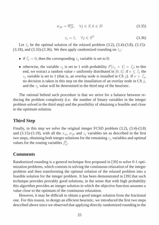
Let zj be the optimal solution of the relaxed problem (3.2), (3.4)-(3.8), (3.15)-(3.18), and (3.33)-(3.36). We then apply randomized rounding on zj :

• if zj = 0, then the corresponding zj variable is set to 0;

• otherwise, the variable zj is set to 1 with probability P [zj = 1] = zj ; to thisend, we extract a random value v uniformly distributed in [0, 1]: if v ≤ zj thezj variable is set to 1 (that is, an overlay node is installed in CS j). If v > zj ,no decision is taken in this step on the installation of an overlay node in CS j,and the zj value will be determined in the third step of the heuristic.

The rational behind such procedure is that we strive for a balance between re-ducing the problem complexity (i.e. the number of binary variables in the integerproblem solved in the third step) and the possibility of obtaining a feasible and closeto the optimum solution.

Third Step

Finally, in this step we solve the original integer FCSD problem (3.2), (3.4)-(3.8)and (3.15)-(3.19), with all the xij , wjk and zj variables set as described in the firsttwo steps, obtaining both integer solutions for the remaining zj variables and optimalvalues for the routing variables f k

ij .

Comments

Randomized rounding is a general technique first proposed in [39] to solve 0-1 opti-mization problems, which consists in solving the continuous relaxation of the integerproblem and then transforming the optimal solution of the relaxed problem into afeasible solution for the integer problem. It has been demonstrated in [39] that suchtechnique provides provably good solutions, in the sense that with high probabilitythis algorithm provides an integer solution in which the objective function assumes avalue close to the optimum of the continuous relaxation.

However, it may be difficult to obtain a good integer solution from the fractionalone. For this reason, to design an efficient heuristic, we introduced the first two stepsdescribed above since we observed that applying directly randomized rounding to the

25

fractional variables of the relaxed FCSD problem leads very often to unfeasible solu-tions where several constraints are violated; then, the computation of a feasible andnear to the optimum solution is not very efficient even applying scaling techniquesas proposed in [39].

Note that in the first step several optimal solutions may exist to the access cov-erage and distribution sub-problems, and it is therefore interesting to extend the H-FCSD algorithm considering different initial solutions. This can also increase theprobability that a feasible solution is obtained in the third step. Obviously, there ex-ists a trade-off between the execution time of the heuristic (which grows with thenumber of different initial solutions considered) and the improvement in the totalnetwork cost. To evaluate this issue we performed several tests, considering up to15 initial solutions, and we found that in all the considered network scenarios themaximum improvement obtained in the cost of the planned SON was less than 2%.For this reason, in Chapter 4 we report numerical results obtained considering onlyone optimal solution in the first step of the H-FCSD heuristic.

3.3.2 H-PMSD: a Heuristic to solve the Profit Maximization SONDesign Problem

In general, determining the optimal subset of end-users to cover in order to maximizethe SON operator’s profit is a more difficult problem than designing the minimumcost overlay network that provides full coverage to a given set of users.

The H-PMSD heuristic tackles such difficulty determining preliminarily whichusers to serve, and then designing the minimum cost SON that covers such users.H-PMSD is therefore composed of two steps, as illustrated in the flow diagram ofFigure 3.2 and detailed in the following.

First Step: determining which users to cover

In this step, a continuous relaxation of the PMSD problem is solved. Let xij be theoptimal solution for the TPs assignment variables. Then, for each TP i we considerthe quantity Qi =

∑j∈S xij , which assumes values in the [0, 1] interval and can

be interpreted intuitively as the probability with which the ith Test Point should becovered by the SON. We then perform randomized rounding on Qi: a random valuev uniformly distributed in [0, 1] is extracted; if v ≤ Qi, then TP i is selected to becovered by the SON; otherwise, TP i is not selected. Let I c ⊆ I be the subset of TPschosen in this step to be covered by the SON.

26

Solve the continuous relaxationof the PMSD problem

For each TP i apply randomizedrounding to the quantity

Determine the minimum cost SONthat covers all TPs in Ic

using the H-FCSD heuristic

Determine the assignment variables

ijx

Determine the subset Ic ofTPs that is convenient to cover

Sj iji xQ ˆ

1st step

2nd step

Figure 3.2: Flow diagram of the H-PMSD heuristic.

Second Step: designing the minimum cost SON

In this step we use the H-FCSD heuristic to design the minimum cost SON thatcovers all the TPs ∈ Ic chosen in the previous step.

Note that the heuristic may be unable to find any feasible solution of the problemsince the cost for covering the selected TPs is higher than the revenue.

H-PMSD with Budget constraints

A cost budget constraint can be taken into account in the first step of the H-PMSDheuristic, introducing constraint (3.22) in the continuous relaxation of the PMSDproblem. With B the budget, if the cost of the SON planned in the second step isnot greater than B, then the computed solution is acceptable. Otherwise, to obtaina feasible solution we apply a scaling technique [39] in the randomized roundingprocedure of the first step. Such technique consists in multiplying the solution of therelaxed problem by a factor γ < 1, which corresponds to using γQi in the first stepof H-PMSD. If γ decreases, the probability that user i is covered by the SON, andas a consequence the total network cost, is reduced until the budget constraint is notviolated.

27

In our work we perform a simple iterative procedure that proceeds as follows:

1. Initialize γ = 1

2. Solve the first step of H-PMSD using γQi

3. Solve the second step of H-PMSD

4. If the cost of the SON planned in the second step of H-PMSD is ≤ B thenSTOP (a feasible solution has been obtained). Otherwise reduce the γ value by0.1 and go to 2)

However, a finer tuning of the γ parameter could be performed, using for examplea binary search technique, to find the γ value which guarantees at the same timefeasibility and a good quality of the solution.

28

Chapter 4

Service Overlay Networks Design:Performance Evaluation

In this Chapter we evaluate the performance of the models and heuristics illustratedin the previous Chapter using a set of realistic and large-size instances, and discussthe effect of different parameters on the characteristics of the planned networks.

More specifically, we test the sensitivity of our models and heuristics to differentparameters like the number of candidate sites and test points, the traffic demands,the installation costs as well as the revenue obtained by covering end-users and theSON operator’s budget. We compare the performance of the exact and heuristicapproaches in terms of the obtained results and computing time. We also providebounds to the performance achievable by any optimization algorithm solving contin-uous relaxations of the integer models.

To this end we consider both randomly generated network instances and real ISPtopologies mapped by the Rocketfuel tool [40, 41]. Random network topologiesare obtained using a custom generator as well as hierarchical (Transit-Stub) modelsgenerated by the GT-ITM topology generator [42, 43], and finally using a degree-based generator (BRITE [44, 45]) to obtain topologies with node degree power laws.

This Chapter is structured as follows: Section 4.1 illustrates the parameters set-tings as well as the random topology generators used in our numerical results. InSection 4.2 we discuss the numerical results obtained by the user assignment andtraffic routing models. Finally, in Section 4.3 we analyze the results of the SONdesign models and heuristics, providing a thorough comparison with the user assign-ment and routing models.

29

4.1 Random Topology Generators and ParametersSetting

To generate random network instances, we have implemented a topology generatorwhich considers a square area with edge equal to 1000, and randomly extracts theposition of m Candidate Sites (CSs), n Test Points (TPs) and p Destination Nodes(DNs). The area is divided into N Internet Service Providers (ISPs); for sake ofsimplicity in this Chapter we consider N = 25 ISPs obtained dividing the wholearea into L × L squares, with L = 200. The same procedure is used to generatenetwork instances with r overlay nodes for the model where their position is given.

Unless stated otherwise, we assume that each TP and DN can be connected toa CS only if the CS is at a distance not greater than 100 from the TP or DN.

As for the connectivity parameters between different CSs, we assume that eachCS can be directly connected with an overlay link to any other CS (i.e., bjl =1, ∀j, l ∈ S); this allows our models to investigate all possible link configurationsto find the optimal overlay topology.

The cost matrix for bandwidth (cBjl) is then generated. If CSs j and l belong to

the same ISP, we assume that cBjl is fixed and equal to 1 monetary unit per Mb/s. On

the other hand, if CSs j and l belong to different ISPs, cBjl depends on the peering

agreements between such ISPs. For the sake of simplicity, we assume that in thiscase cB

jl is a random variable uniformly distributed between C/2 and 3C/2, with C

being equal to Ljl

L, that is the distance between j and l (Ljl) divided by the width of

an ISP domain (L), i.e. 200 with the above settings.If not specified differently, the installation cost of an overlay node is equal to 10

monetary units. As for the access and egress cost, we assume they are fixed and equalto 1 monetary unit per Mb/s.

The maximum capacity that can be reserved between CSs j and l on the overlaylink (j, l) ujl, j, l ∈ S is set equal to 50 Mb/s, as well as the maximum capacity of theaccess link of CS j, vj, j ∈ S. The capacity of the egress links connecting overlaynodes to destination nodes is hjk = 100 Mb/s, for all j ∈ S and k ∈ D.

Obviously, none of the above assumptions affects the proposed models and heuris-tics which are general and can be applied to any problem instance and network topol-ogy.

Identifying Candidate Sites can be a difficult task in real ISPs networks. To solvethis problem, a topology-aware node placement heuristic could be used, as proposedin [9], to decide the potential locations for overlay nodes inside an ISP. Such tech-niques can be used together with our heuristics and models, thus representing a fur-ther research topic worth pursuing.

30

All the results reported hereafter are the optimal and approximate solutions ofthe considered instances obtained, respectively, by formalizing the proposed modelsin AMPL [46] (see Appendix A.3) and solving them with CPLEX [47], or using theproposed heuristics, on workstations equipped with an Intel Pentium 4 (TM) proces-sor with CPUs operating at 3 GHz, and with 1024 Mbyte of RAM. For each networkscenario, the results are obtained averaging each point on 10 network instances.

4.2 User Assignment and Routing Models

We first tackle the user assignment and routing problem, considering different net-work scenarios and varying several parameters such as the number of overlay nodes,the traffic demands, the gain the SON operator obtains serving end-users and the costbudget.

a) Effect of the Traffic Demands: Random network instances

We first consider the Full Coverage User Assignment and Routing model (FC-UAR)in a random network scenario with n = 20 TPs and p = 20 DNs. Each test pointoffers the same amount of traffic dik to all destination nodes.

Figure 4.1 reports an example of the planned networks when applying the FC-UAR model to the same instance with r = 40 overlay nodes and with two differentrequirements on the end-user traffic, dik = 500 kb/s and dik = 2 Mb/s for all TPs andDNs. Overlay nodes, TPs and DNs are represented respectively by circles, trianglesand squares. We observe that increasing the traffic demands forces the model to use ahigher number of overlay nodes and to install more links to convey the traffic towardsthe destination nodes.

Table 4.1 analyzes the characteristics of the solutions in the same scenario whenvarying the number of overlay nodes r. For each couple (r, dik) we report the num-ber of installed overlay links (NL), the network cost (i.e. the value of the objectivefunction (3.1), page 16) and the processing time to get the optimal solution.

Table 4.1 suggests three main comments. First, the very same effect of trafficincrease observed in Figure 4.1 is evident also in averaged results. In fact, owingto capacity constraints, just increasing the link bandwidth is not sufficient and it isnecessary to use more overlay nodes and links. Second, for a given traffic value,increasing the number of overlay nodes (r) in the FC-UAR model increases the solu-tion space; as a consequence, the model favors the solutions providing connectivityat a lower cost, which in turn decreases with r.

31

0

200

400

600

800

1000

0 200 400 600 800 1000

(a) 500 kb/s

0

200

400

600

800

1000

0 200 400 600 800 1000

(b) 2 Mb/s

Figure 4.1: Sample SONs planned by the FC-UAR model with increasing trafficdemands (500 kb/s and 2 Mb/s). The number of TPs and DNs is 20, while the numberof overlay nodes is 40. Overlay nodes, TPs and DNs are represented respectively bycircles, triangles and squares.

32

Table 4.1: Solutions provided by the FC-UAR model with 20 TPs and DNs.dik=500 kb/s dik=1000 kb/s

r NL Cost Time (s) NL Cost Time (s)30 184.6 783.1 0.5 195.8 1568.9 0.640 217.3 765.6 1.2 231.4 1532.7 1.250 239.8 746.8 2.2 249.4 1494.6 2.3

100 305.7 698.0 23.6 320.4 1395.6 22.8200 414.6 661.6 220.9 431.9 1323.5 223.4300 452.3 643.3 718.3 470.8 1285.9 765.7

Finally, it can be noted that the FC-UAR model solves the user assignment androuting problem even for large-scale network instances with a short computing time.

We then simulated a scenario with a higher number of traffic flows, considering100 TPs and 10 DNs, where DNs can be seen as acting like concentrator nodes oraccess points to other networks. The results obtained with the FC-UAR model areshown in Table 4.2 with r ranging from 30 to 300 and for different dik values, andthey are in line with the observations reported above.

Table 4.2: Solutions provided by the FC-UAR model with 100 TPs and 10 DNs.dik=20 kb/s dik=40 kb/s

r NL Cost Time (s) NL Cost Time (s)30 260.5 77.3 0.2 260.5 154.7 0.240 290.8 74.7 0.3 290.9 149.4 0.350 323.7 73.2 0.6 324.0 146.4 0.6

100 425.1 69.0 5.9 425.2 138.1 5.8200 547.0 65.8 68.0 547.1 131.5 68.2300 631.7 64.2 239.8 631.9 128.3 242.8

b) Effect of the Traffic Demands: Transit-Stub topologies

To investigate the behavior of the FC-UAR model with a large number of trafficflows, we generated large-scale Transit-Stub topologies using GT-ITM [42].

In such scenarios, the Internet is modeled as a collection of interconnected rout-ing domains, which can be classified as either Transit domains (that contain backbone

33

nodes) or Stub domains (which have one or more gateway nodes that are connectedto transit domains).

We considered 10 random Transit-Stub topologies with r = 50, 100, 200 overlaynodes and an average number of links equal to 400, 550 and 1200, respectively,including access and egress links; each link can be selected as an overlay link. Foreach topology we generated 10 random distributions of n = 100 TPs and p = 100DNs, where each TP offers the same amount of traffic dik = 10 kb/s to all destinationnodes. All other parameters are the same as in the previous network scenarios.

The numerical results obtained with the FC-UAR model, averaged over all net-work topologies and random TPs/DNs distributions, are shown in Table 4.3. Weobserve that owing to the hierarchical structure of Transit-Stub topologies, a largenumber of overlay links is selected in the planned SON; furthermore, the time nec-essary to compute the optimal solution is very short.

Table 4.3: Transit-Stub topologies: solutions provided by the FC-UAR model with100 TPs, 100 DNs and dik=10 kb/s.

r NL Cost Time (s)50 341.9 700.0 0.5

100 418.6 873.8 5.7200 449.6 1040.4 10.5

c) Effect of the Gain parameter on Profit Maximization

We evaluate the effect of the gain parameter on the Profit Maximization User As-signment and Routing model (PM-UAR) considering a scenario with 50 TPs, 50DNs and r = 100 overlay nodes. We assume that the gain per bandwidth unit thatthe SON operator obtains for serving an end-user (the parameter gi in the objectivefunction (3.12), page 18) is a random variable with average equal to G and a uniformdistribution between G/2 and 3G/2, with G ranging between 0 and 0.01 monetaryunits per Mb/s.

Figure 4.2 shows the number of end-users covered by the SON as a function ofG. Obviously, for small G values, the SON is not profitable enough to cover any ofthe end-users; as G increases, the SON covers more end-users, and eventually all ofthem. Similar results have been observed with different values of r.

Table 4.4 reports, for the same scenario, the number of installed links, the SONoperator’s profit (i.e. the value of the objective function (3.12)), the network cost

34

and processing time, as a function of G. Note that when G increases, the plannednetwork covers more end-users, and as a consequence it uses more overlay links.

0 0.002 0.004 0.006 0.008 0.010

5

10

15

20

25

30

35

40

45

50

Average Gain per Mb/s

Num

ber

of U

sers

Figure 4.2: Number of end-users covered by the SON as a function of the averagegain per bandwidth unit (PM-UAR model), with 50 TPs, 50 DNs, 100 overlay nodesand dik=100 kb/s.

Table 4.4: Solutions provided by the PM-UAR model with 50 TPs and DNs, 100overlay nodes and dik=100 kb/s.

G NL Profit Cost Time (s)0.005 703.3 383.7 682.1 42.20.006 755.7 608.7 792.6 42.10.007 771.4 847.7 847.6 42.00.008 780.7 1091.6 865.2 41.90.009 780.8 1336.2 865.2 42.00.010 780.9 1580.8 865.2 41.8

35

d) Effect of the Budget parameter

Finally, to evaluate the effect that a budget constraint has on the planning of an SON,we consider several budget (B) values in the 500 to 1000 range, solving the PM-UAR model in a random network scenario with 20 TPs and DNs, 40 overlay nodesand dik=500 kb/s.

Figure 4.3 illustrates the number of end-users covered by the SON as a functionof the operator’s budget, for different G values. For each value of G, as the budgetincreases, the number of end-users accepted in the network increases until it reachesits maximum.

Table 4.5 reports in detail the characteristics of the solutions provided by thePM-UAR model in such a scenario, for G = 0.01 monetary units per Mb/s and fordifferent budget values. The results show that deploying higher-cost networks allowsthe SON operator to achieve higher network profits. This, however, also increases theeconomic risk faced by the SON operator in the deployment of the overlay network.

500 600 700 800 900 100010

11

12

13

14

15

16

17

18

19

20

SON Operator Budget

Num

ber

of U

sers

G=0.005G=0.006G=0.007G=0.008G=0.009G=0.010

Figure 4.3: Number of end-users covered by the SON as a function of the budget fordifferent values of the average gain per bandwidth unit G (PM-UAR model), with 20TPs, 20 DNs and 40 overlay nodes.

36

Table 4.5: Solutions provided by the PM-UAR model with 20 TPs and DNs, 40overlay nodes, G=0.01 monetary units per Mb/s and dik=500 kb/s.

B Users NL Profit Cost Time (s)500 13.0 175.1 1015.3 492.8 40.2600 15.4 192.7 1118.3 583.8 37.4700 18.0 209.0 1203.2 686.9 33.7800 20.0 217.4 1241.6 765.6 2.8900 20.0 217.4 1241.6 765.6 2.7

1000 20.0 217.4 1241.6 765.6 2.7

4.3 Network Design Models and Heuristics

We now present the results of the SON design models, providing a thorough com-parison with the continuous relaxation, the proposed heuristics as well as the userassignment and routing models. Also in this case we analyze the impact on theplanned overlay networks of traffic demands, installation and bandwidth costs, gainand budget parameters.


To gauge the effect of the traffic demands on the Full Coverage SON Design (FCSD)model, let us consider a random network scenario with n = 20 TPs, p = 20 DNs anda variable number of Candidate Sites, m. Each test point offers the same amount oftraffic dik to all destination nodes.

Figure 4.4 reports an example of the planned networks when applying the FCSDmodel to the same instance with m = 40 candidate sites and with two differentrequirements on the end-user traffic, dik = 500 kb/s and dik = 1 Mb/s for all TPsand DNs. CSs, TPs and DNs are represented with circles, triangles and squares,respectively. As expected, increasing the traffic demands forces the model to install ahigher number of overlay nodes and links to convey the traffic towards the destinationnodes.

Table 4.6 analyzes the characteristics of the solutions of the FCSD model, itscontinuous relaxation and the H-FCSD heuristic in the same scenario when varyingthe number of candidate sites.

For each couple (m, dik) and optimization algorithm, the Table reports the num-ber of installed overlay nodes (NR) and links (NL), the total network cost and thecomputing time (measured in seconds) to obtain the solution.

37

(a) 500 kb/s

(b) 1000 kb/s

Figure 4.4: Sample SONs planned by the FCSD model with increasing traffic de-mands (500 and 1000 kb/s). The number of TPs and DNs is 20, while the numberof CSs is 40. CSs, TPs and DNs are represented with circles, triangles and squares,respectively.

38

For small instances we could obtain the exact solutions with the FCSD model,which enabled a comparison between the H-FCSD heuristic and optimal integer solu-tions; column gapI reports the percentage gap between the cost provided by H-FCSDand the optimal cost obtained with the FCSD model. This gap shows how close isH-FCSD to the optimum obtained by FCSD, in terms of the objective function value.

We also reported the results obtained solving the continuous relaxation of theFCSD model, which provides a lower bound on the network cost that can be ob-tained with any optimization algorithm; column gapB shows the percentage gap be-tween the cost provided by the H-FCSD heuristic and such lower bound. Note thatsuch relaxation is used exclusively to provide a reference point, especially for largenetwork instances where solutions using FCSD cannot be obtained.

Finally, column gapL shows the percentage gap between the cost provided by theFCSD model and that obtained solving the continuous relaxation of FCSD. Thus,gapL measures how far is the optimal integer solution from the relaxed one.

Three main results come from the observation of the Table: first, the very sameeffect of traffic increase observed in Figure 4.4 is evident also on averaged results;in fact, the number of installed nodes and links increases when increasing the trafficdemands.

Second, for a given traffic value, increasing the number of CSs (m) increases thesolution space; as a consequence, the model favors the solutions providing connec-tivity that have a lower impact on the network cost, which in turn decreases with m.

Finally, the proposed heuristic performs very close to the optimal solutions (lessthan 4.2% for dik = 500 kb/s and less than 3.1% for dik = 1 Mb/s), and in all casesthe computation time is below 30 seconds for all the tested instances. Even whencompared to the bound provided by the continuous relaxation, the performance gapis less than 20% in all network scenarios.

Since for small network sizes (m = 30, 40, 50) it can be observed that gapI issignificantly smaller than gapB , we can guess that even for larger topologies (whereFCSD cannot be solved and consequently gapI cannot be computed) H-FCSD per-forms considerably closer to the optimal integer solution than what is indicated bythe gapB value.

We further observe that the gapL value is quite small (less than 10%) for all net-work instances, which motivates the choice to use the continuous relaxation in ourheuristics as a basis to obtain good integer solutions applying the randomized round-ing technique.

To compare the results obtained with FCSD with those of the FC-UAR model,we assume that the set S of candidate sites considered in FCSD is the same as theset R of overlay nodes used in FC-UAR (as a consequence, m = r). In this way,

39

Tabl

e4.

6:So

lutio

nspr

ovid

edby

the

FCSD

mod

el,t

heFC

SDco

ntin

uous

rela

xatio

nan

dth

eH

-FC

SDhe

uris

tic,w

ith20

TPs

and

20D

Ns.

dik

=50

0kb

/sFC

SDFC

SDC

ontin

uous

Rel

axat

ion

H-F

CSD

mN

RN

LC

ost

Tim

egap

L%

NR

NL

Cos

tT

ime

NR

NL

Cos

tT

ime

gap

I%

gap B

%30

19.6

150.

110

01.3

12.4

7.72

13.8

205.

392

9.5

0.3

19.8

146.

310

32.0

0.5

3.07

11.0

340

19.2

146.

699

3.2

244.

89.

0813

.926

9.5

910.

50.

721

.015

4.2

1025

.91.

33.

2912

.67

5019

.514

8.3

981.

946

65.8

9.71

13.9

321.

289

5.0

1.8

21.4

153.

710

22.6

1.6

4.15

14.2

660

13.8

380.

687

9.8

3.2

22.2

160.

010

18.2

3.2

15.7

380

13.7

491.

585

8.3

10.9

23.3

163.

510

17.9

8.2

18.5

910

013

.760

3.4

845.

528

.023

.616

3.1

1013

.415

.919

.86

dik

=10

00kb

/sFC

SDFC

SDC

ontin

uous

Rel

axat

ion

H-F

CSD

mN

RN

LC

ost

Tim

egap

L%

NR

NL

Cos

tT

ime

NR

NL

Cos

tT

ime

gap

I%

gap B

%30

21.7

167.

818

13.4

5.6

4.54

15.5

208.

217

34.6

0.3

22.2

165.

818

30.8

0.6

0.96

5.55

4022

.717

4.8

1795

.165

.35.

7215

.926

6.3

1697

.90.

723

.217

3.2

1829

.91.

31.

947.

7750

22.9

175.

117

76.1

3655

.56.

6015

.832

4.1

1666

.21.

924

.617

8.3

1829

.53.

53.

019.

8060

15.8

380.

616

39.6

3.2

26.1

187.

018

23.2

6.3

11.2

080

15.4

492.

715

93.7

11.0

27.2

187.

818

21.3

13.2

14.2

810

015

.559

5.5

1568

.027

.728

.019

0.5

1817

.530

.015

.91

40

the solution of the FCSD model measures the advantage obtained by optimizing thenumber and position of the installed overlay nodes, in addition to the user assign-ment and traffic routing optimization performed by the FC-UAR model. For the sakeof comparison we also added two columns in Table 4.7 that show the network costachieved with the FC-UAR model and the percentage gap (gapc) between the costprovided by the FCSD model and that obtained solving FC-UAR. To make a faircomparison between the two models, in the Table we reported for FC-UAR the ob-jective function value (3.1) increased by the cost necessary to install r overlay nodes(r · 10 monetary units, with the settings used in this scenario). Table 4.7 reports thenumber of installed overlay nodes (NR), overlay links (NL), the total network costand the processing time to get the optimal solution. We note that the gap between thecosts obtained with FC-UAR and FCSD is remarkable and it increases with increas-ing m values.

Table 4.7: Solutions provided by the FCSD model with 20 TPs and 20 DNs.dik=500 kb/s

FCSD FC-UARm NR NL Cost Time (s) Cost gapc(%)30 19.6 150.1 1001.3 12.4 1086.8 8.540 19.2 146.6 993.2 244.8 1172.9 18.150 19.5 148.3 981.9 4665.8 1246.8 27.0

dik=1000 kb/sFCSD FC-UAR

m NR NL Cost Time (s) Cost gapc(%)30 21.7 167.8 1813.4 5.6 1879.2 3.640 22.7 174.8 1795.1 65.3 2119.7 18.150 22.9 175.1 1776.1 3655.5 2185.4 23.0

We also simulated large-scale network scenarios with n = 100 TPs and p = 10DNs, which can be seen as acting like concentrator nodes or access points towardsother networks.

The results obtained with the H-FCSD heuristic and the continuous relaxationof the FCSD model are shown in Table 4.8, with m ranging from 100 to 300 andfor different dik values (viz. 20 kb/s and 40 kb/s), and they are in line with theobservations reported above.

41

Table 4.8: Large-size instances: solutions provided by the FCSD continuous relax-ation and the H-FCSD heuristic, with 100 TPs and 10 DNs.

dik=20 kb/sFCSD Continuous Relaxation H-FCSD

m NR NL Cost Time NR NL Cost Time gapB %100 23.3 570.1 303.7 7.3 27.3 241.9 351.1 4.8 15.61200 21.7 1036.0 284.8 128.9 27.2 236.3 350.0 58.8 22.89300 20.8 1564.9 274.7 792.1 27.1 236.3 348.2 241.8 26.76

dik=40 kb/sFCSD Continuous Relaxation H-FCSD

m NR NL Cost Time NR NL Cost Time gapB %100 23.4 570.8 374.8 7.6 27.4 242.3 429.8 4.8 14.67200 21.8 1035.1 353.5 131.3 27.4 237.6 429.7 57.9 21.56300 20.9 1567.6 342.1 979.9 27.1 236.3 425.8 248.4 24.47

On the other hand, the results summarized in Table 4.9, are obtained with theFCSD and FC-UAR models, with n = 100 TPs and p = 10 DNs, m ranging from30 to 50 overlay nodes and for dik= 20 kb/s and 40 kb/s, and they are also in linewith what was reported above. In this case the processing time to obtain the optimalsolutions is almost negligible.

A variation of the above scenarios is further considered, where the offered trafficis not constant, but uniformly distributed at random between 1

2dik and 3

2dik. We ob-

served that the results obtained are very close to those reported in Tables 4.6 and 4.8,with a maximum gap inferior to 1%.

b) Effect of the Traffic Demands: Transit-Stub topologies

To evaluate the behavior of the FCSD model with Transit-Stub topologies, we con-sidered the same scenarios illustrated previously for FC-UAR.

The numerical results obtained with the FCSD model, its continuous relaxationand the H-FCSD heuristic, averaged over all network topologies and random TPs/DNsdistributions, are shown in Table 4.10. It can be seen that due to the hierarchicalstructure of Transit-Stub topologies, a large number of overlay links is selected inthe planned SON. Moreover, even in this scenario H-FCSD performs close to theoptimal solution provided by the FCSD model.

If now we compare the results of the FCSD model with those obtained with FC-

42

Table 4.9: Solutions provided by the FCSD model with 100 TPs and 10 DNs.





UAR (Tables 4.3 and 4.11), we can observe that the FCSD model installs, in average,considerably fewer overlay nodes and links than FC-UAR, thus reducing consistentlythe cost of the planned network.

Table 4.10: Transit-Stub topologies: solutions provided by the FCSD model, the FCSD con-tinuous relaxation and the H-FCSD heuristic, with 100 TPs, 100 DNs, 100 CSs and dik=10kb/s.

FCSD FCSD Continuous Relaxation H-FCSDNR NL Cost Time gapL % NR NL Cost Time NR NL Cost Time gapI % gapB %

38.0 338.1 1272.4 484.1 7.61 27.5 508.8 1182.4 5.3 48.5 347.2 1434.1 1.5 12.71 21.29

c) Effect of the Traffic Demands: Power Law topologies

To better capture the power law distributions for node degrees that characterize In-ternet topologies, we further considered BRITE, a degree-based topology generator[44, 45]. BRITE was used to generate power law topologies with 100 CSs, 20 TPsand 20 DNs on a square area with edge equal to 1000; the Barabasi − Albert model[48] was adopted with default parameters provided by BRITE.

43

Table 4.11: Transit-Stub topologies: solutions provided by the FCSD model with100 TPs, 100 DNs and dik=10 kb/s.

FCSD FC-UARm NR NL Cost Time (s) Cost gapc(%)50 25.3 310.9 954.6 1.6 1200.0 25.7

100 38.0 338.1 1272.4 484.1 1873.8 47.3200 72.3 386.9 1768.7 2436.0 3040.4 71.9

The area was divided into N = 25 ISPs, each occupying an L × L square, withL = 200. Moreover, the bandwidth cost matrix was generated as for the customtopology generator.

Table 4.12 reports the numerical results obtained with such topologies, with anoffered traffic dik equal to 500 and 1000 kb/s. The results confirm the behavior al-ready observed for the random instances obtained with the custom generator, wherethe number of installed overlay nodes and links increases with increasing traffic de-mands. H-FCSD plans SON topologies with a reasonable cost in a very short com-puting time, which is almost independent of the traffic offered to the network.

Table 4.12: Power Law topologies: solutions provided by the FCSD model, the FCSDcontinuous relaxation and the H-FCSD heuristic in the topologies with node degree powerlaws generated using BRITE, with 100 CSs, 20 TPs and 20 DNs.

FCSD FCSD Continuous Relaxation H-FCSDdik NR NL Cost Time gapL % NR NL Cost Time NR NL Cost Time gapI % gapB %500 17.1 87.8 987.9 70.1 11.58 11.3 146.0 885.4 0.6 22.5 96.6 1272.7 0.3 28.83 43.74

1000 24.4 110.7 2022.8 48.8 12.18 15.3 155.9 1803.2 0.7 29.6 119.6 2583.2 0.4 27.70 43.26

d) Effect of the Traffic Demands: Rocketfuel topologies

We considered four diverse ISP backbone topologies, listed in Table 4.13, collectedby Rocketfuel [40, 41], an Internet mapping tool.

In such topologies, all routers can be selected to install overlay nodes and all linkscan be selected as overlay links. The cost of each overlay link was set proportionalto its length. For each topology we generated 10 random distributions of n = 20TPs and p = 20 DNs, where each TP offers the same amount of traffic dik to alldestination nodes. All other parameters are the same as in the previous networkscenarios.

44

Table 4.13: Rocketfuel-inferred ISP topologies: number of backbone routers andlinks (including access and egress links).

Network Location Routers LinksEbone EU 88 362Tiscali EU 164 696Exodus US 80 334

Abovenet US 145 788

The numerical results, averaged over all network topologies and random TPs/DNsdistributions, are shown in Table 4.14 for dik = 500 and 1000 kb/s.

For these topologies we further measured the average length of the paths chosenby the FCSD model to route traffic flows; the path length is expressed in terms of thenumber of hops traversed by the flow (Hop Count, HC). Such performance figure isreported in the last column of Table 4.14.

Note that in all such real scenarios the proposed heuristic performs very well andclose to the optimum, thus representing a practical solution for the planning of SONs.Furthermore, the average path length increases with increasing traffic demands, sincean increasing fraction of the offered traffic must be routed on longer (and generallycostlier) paths due to capacity constraints.

e) Effect of the Installation and Bandwidth Reservation Costs

We evaluate the effect of the bandwidth cost as well as the nodes’ installation cost onour models’ performance, considering a random network scenario with n = p = 20TPs and DNs and m = 50 CSs. The offered traffic dik is equal to 500 kb/s. Thesolution, and in particular the number of installed nodes and links, intuitively de-pends on two factors: the ratio β between the overlay nodes’ installation cost and thebandwidth reservation cost, and the ratio δ between the cost of a link connecting twoCSs which belong to different ISPs and that of a link connecting two CSs belongingto the same ISP.

Tables 4.15 and 4.16 report the results obtained varying, respectively, the param-eters β and δ. Table 4.15 shows that if the cost of installing an overlay node decreaseswith respect to the bandwidth reservation cost, the proposed models and heuristicstend to install more overlay nodes.

Note that the computing time of the H-FCSD heuristic is very short and the ap-proximate solution is very close to the optimal solution provided by the FCSD model.Moreover, when β diminishes, the performance gap between H-FCSD and both the

45

Tabl

e4.

14:

Roc

ketf

uelt

opol

ogie

s:so

lutio

nspr

ovid

edby

the

FCSD

mod

el,t

heFC

SDco

ntin

uous

rela

xatio

nan

dth

eH

-FC

SDhe

uris

tic,w

ith20

TPs

and

20D

Ns.

dik

=50

0kb

/sFC

SDFC

SDC

ontin

uous

Rel

axat

ion

H-F

CSD

Net

wor

kN

RN

LC

ost

Tim

egap

LN

RN

LC

ost

Tim

eN

RN

LC

ost

Tim

egap

Igap B

HC

Ebo

ne26

.811

5.6

2150

.310

5.4

7.43

15.8

171.

220

01.6

0.4

34.9

135.

024

18.0

0.3

12.4

520

.80

4.96

Tis

cali

26.7

111.

420

21.3

79.2

7.72

16.3

184.

518

76.5

0.6

34.5

128.

523

94.4

0.4

18.4

627

.60

5.14

Exo

dus

25.8

116.

334

32.9

36.3

4.32

14.2

159.

132

90.8

0.4

32.4

131.

337

29.6

0.3

8.64

13.3

34.

33A

bove

net

24.0

114.

050

71.2

193.

92.

4913

.921

5.2

4948

.01.

033

.513

5.6

5605

.90.

710

.54

13.3

04.

74

dik

=10

00kb

/sFC

SDFC

SDC

ontin

uous

Rel

axat

ion

H-F

CSD

Net

wor

kN

RN

LC

ost

Tim

egap

LN

RN

LC

ost

Tim

eN

RN

LC

ost

Tim

egap

Igap B

HC

Ebo

ne32

.113

5.5

4069

.38.

34.

8320

.417

5.0

3907

.40.

641

.515

5.9

4438

.60.

38.

3613

.59

5.17

Tis

cali

32.1

135.

438

13.7

20.7

4.80

20.7

183.

836

39.0

0.6

41.5

156.

144

08.7

0.5

15.6

021

.15

5.30

Exo

dus

30.3

134.

066

59.0

5.4

2.55

19.1

160.

164

93.4

0.5

37.5

152.

171

70.5

0.2

7.68

10.4

34.

55A

bove

net

29.8

138.

599

96.8

27.4

1.79

17.1

223.

398

21.0

1.0

40.4

166.

411

057.

50.

610

.61

12.5

94.

92

46

FCSD model and the lower bound greatly decreases.Similarly, when δ increases, we observed that our model and heuristic tend to

deploy more overlay nodes and links; the majority of these links connect overlaynodes belonging to the same ISP, thus diminishing the number of longer (and costlier)links that traverse different ISPs in the planned SON. This behavior is reflected in thenumerical results reported in Table 4.16.

Table 4.15: Variable cost ratio β: solutions provided by the FCSD model, the FCSD con-tinuous relaxation and the H-FCSD heuristic with 20 TPs, 20 DNs, 50 CSs and dik=500kb/s.

FCSD FCSD Continuous Relaxation H-FCSDβ NR NL Cost Time gapL % NR NL Cost Time NR NL Cost Time gapI % gapB %10 19.5 148.3 981.9 4665.8 9.71 13.9 321.2 895.0 1.5 21.4 153.8 1018.2 1.6 3.70 13.771 30.8 209.9 783.5 108.9 2.45 16.0 266.5 764.8 1.3 31.4 192.7 800.6 1.3 2.18 4.68

1/10 50.0 239.6 748.5 1.7 0.00 50.0 239.4 748.5 1.1 50.0 237.8 762.2 1.6 1.83 1.83

Moreover, Table 4.17 illustrates the effect of the costs in a network scenario with20 TPs, 20 DNs, 40 CSs and dik = 500 kb/s. These results are in line with thosereported in Table 4.14. For comparison, the results obtained with FC-UAR are alsoreported in the last row of the Table since they represent a bound for FCSD corre-sponding to a negligible cost of the overlay nodes.

f) Effect of the Gain parameter

We then evaluate the Profit Maximization SON Design problem, considering a ran-dom network scenario with 20 TPs, 20 DNs, m = 40 CSs and offered traffic dik=500kb/s. We assume, as for PM-UAR, that the gain per bandwidth unit gi is a randomvariable with average equal to G and a uniform distribution between G/2 and 3G/2,where G ranges between 0 and 0.01 monetary units per Mb/s.

Figure 4.5 reports an example of the planned networks when applying the PMSDmodel to the same instance considered in Figure 4.4 with m = 40 CSs and with twodifferent requirements on the end-user traffic, dik = 500 kb/s and dik = 1 Mb/s forall TPs and DNs; G is equal to 0.005 monetary units per Mb/s. CSs, TPs and DNs arerepresented with circles, triangles and squares, respectively. In this case the plannedSONs cover only a subset of the TPs to maximize the operator’s profit.

Figure 4.6 shows the number of end-users covered by the SON as a function ofG for both the PMSD model and the H-PMSD heuristic. Note that the two curvesalmost overlap, as the H-PMSD heuristic is quite accurate in determining the optimalnumber of users to serve to maximize the SON operator’s profit. Obviously, forsmall G values, the SON is not profitable enough to cover any of the end-users; as

47

Tabl

e4.

16:

Var

iabl

eco

stra

tioδ:

solu

tions

prov

ided

byth

eFC

SDm

odel

,the

FCSD

cont

inuo

usre

laxa

tion

and

the

H-F

CSD

heur

istic

with

20T

Ps,2

0D

Ns,

50C

Ssan

dd

ik=

500

kb/s

.FC

SDFC

SDC

ontin

uous

Rel

axat

ion

H-F

CSD

δN

RN

LC

ost

Tim

egap

L%

NR

NL

Cos

tT

ime

NR

NL

Cos

tT

ime

gap

I%

gap B

%1

19.5

148.

398

1.9

4665

.89.

7113

.932

1.2

895.

01.

521

.415

3.8

1018

.21.

63.

7013

.77

221

.815

4.3

1355

.913

853.

69.

5014

.532

9.7

1238

.31.

424

.216

2.4

1404

.72.

83.

6013

.44

526

.616

8.8

2356

.070

60.3

7.48

15.1

281.

321

92.0

1.5

30.3

174.

324

41.7

4.7

3.64

11.3

910

31.1

182.

939

25.7

2780

.55.

4615

.625

6.5

3722

.41.

335

.218

4.5

4058

.63.

43.

399.

03

48

Table 4.17: Variable cost ratio β: solutions provided by the FCSD model with 20TPs, 20 DNs, 40 CSs and dik=500 kb/s.

β NR NL Cost Time (s)10 19.3 148.5 987.0 203.41 28.7 197.2 795.3 12.0

1/10 40.0 215.9 767.9 0.7

FC − UAR 40.0 217.3 765.6 1.2

G increases, the SON covers more end-users, eventually all of them. Similar resultshave been observed in several network topologies with a varying number of CSs.

Table 4.18 reports, for the PMSD model, its continuous relaxation and the H-PMSD heuristic, the total number of installed nodes and links, the SON operator’sprofit (i.e., the value of the objective function ((3.20), page 21) or the approximatevalue obtained with H-PMSD) and computing time, as a function of G. Note thatwhen G increases, the planned network covers more end-users, and as a consequenceit comprises more overlay nodes and links.

Column gapI shows the percentage gap between the profit provided by the H-PMSD heuristic and the optimal profit obtained with the PMSD model, while col-umn gapB reports the gap between H-PMSD and the upper bound provided by thecontinuous relaxation of the PMSD model. Column gapL provides the gap betweenthe PMSD model and its continuous relaxation. The performance gap is slightlylarger with respect to the full coverage design problem; this is mainly due to the dif-ficulty in determining the optimal subset of users to cover. However, note that theperformance gap is still largely acceptable since in all cases it is less than 30%, andit greatly decreases with increasing values of G.

Finally, Figure 4.7 compares the number of end-users covered by the SON forthe PMSD and PM-UAR models (r = m) as a function of G. Since the cost ofinstalling overlay nodes is not considered in PM-UAR, such model tends to covermore end-users than PMSD for all G values.

We further tested the H-PMSD heuristic with large-scale network instances. Ta-ble 4.19 reports the numerical results obtained with 50 TPs, 50 DNs, 100 CSs anddik=20 kb/s for both the H-PMSD and the PMSD continuous relaxation. Even in thisnetwork scenario the proposed heuristic provides accurate solutions with a consider-ably reduced computing time.

49

Tabl

e4.

18:

Solu

tions

prov

ided

byth

ePM

SDm

odel

,the

H-P

MSD

heur

istic

and

the

cont

inuo

usre

laxa

tion

with

20T

Psan

dD

Ns,

40C

Ssan

dd

ik=

500

kb/s

.PM

SDPM

SDC

ontin

uous

Rel

axat

ion

H-P

MSD

GN

RN

LPr

ofit

Tim

egap L

%N

RN

LPr

ofit

Tim

eN

RN

LPr

ofit

Tim

egap I

%gap B

%0.

005

15.0

103.

071

.956

0.8

56.5

09.

723

4.1

165.

30.

614

.311

5.5

51.0

1.4

29.0

769

.15

0.00

617

.212

5.7

241.

835

9.5

25.8

111

.224

8.0

325.

90.

617

.912

8.2

213.

11.

511

.87

34.6

10.

007

18.2

138.

042

2.7

326.

116

.31

12.7

261.

850

5.1

0.6

18.6

144.

239

0.0

1.6

7.74

22.7

90.

008

18.9

142.

861

6.3

263.

311

.76

13.4

267.

969

8.4

0.6

20.1

149.

758

5.0

1.5

5.08

16.2

40.

009

19.2

146.

581

4.8

190.

59.

1713

.827

0.7

897.

10.

620

.715

3.4

786.

51.

63.

4712

.33

0.01

019

.214

6.5

1015

.019

5.0

7.51

13.8

270.

710

97.4

0.6

20.7

153.

598

7.4

1.6

2.72

10.0

2

50

(a) 500 kb/s

(b) 1000 kb/s

Figure 4.5: Sample SONs planned by the PMSD model with increasing traffic de-mands (500 and 1000 kb/s). The number of TPs and DNs is 20, while the numberof CSs is 40. The average gain per bandwidth unit, G, is equal to 0.005 monetaryunits per Mb/s. CSs, TPs and DNs are represented with circles, triangles and squares,respectively.

51

0 0.002 0.004 0.006 0.008 0.010

2

4

6

8

10

12

14

16

18

20


Num

ber

of U

sers

PMSD

H−PMSD

Figure 4.6: Number of end-users covered by the SON with the PMSD model and theH-PMSD heuristic as a function of the average gain per bandwidth unit, with 20 TPs,20 DNs, 40 CSs and dik=500 kb/s.

Table 4.19: Large-size instances: solutions provided by the H-PMSD heuristic andthe PMSD continuous relaxation, with 50 TPs, 50 DNs, 100 CSs and dik=20 kb/s.

PMSD Continuous Relaxation H-PMSDG NR NL Profit Time NR NL Profit Time gapB %

0.005 13.6 127.5 213.0 78.8 27.2 269.6 13.2 123.0 92.380.006 16.2 131.3 416.5 71.6 29.0 312.5 215.5 114.6 48.260.007 17.9 134.4 642.0 66.3 29.5 331.5 444.3 111.7 30.790.008 18.8 134.9 879.5 68.9 30.1 342.4 683.6 114.8 22.270.009 19.5 134.3 1120.7 66.3 30.5 351.4 929.3 111.8 17.080.010 19.9 134.4 1363.9 67.2 31.0 361.4 1171.8 111.9 14.08

g) Effect of the Budget parameter

Finally, we evaluate the impact of the budget parameter on the PMSD model consid-ering a random network scenario with 20 TPs and DNs, 40 CSs, dik = 500 kb/s andseveral budget (B) values in the 500 to 1000 range.

52

0 0.002 0.004 0.006 0.008 0.010

2

4

6

8

10

12

14

16

18

20


Num

ber

of U

sers

PMSD

PM−UAR

Figure 4.7: Number of end-users covered by the SON as a function of the averagegain per bandwidth unit, with 20 TPs, 20 DNs and 40 CSs.

Figure 4.8 shows the number of end-users accepted in the SON as a function ofthe budget, for different G values. Similarly to the PM-UAR model, given a G value,the number of end-users covered by the SON increases as the budget increases, untilit reaches its maximum, which can be obtained from Figure 4.6.

For small budget values (B ≤ 700), all curves practically overlap except for thatcorresponding to G = 0.005 monetary units per Mb/s. This is due to the fact that forG > 0.005 the number of users covered by the PMSD model is limited by the budgetconstraint, so that the model chooses the most profitable users that can be accepted inthe SON given the budget value. On the other hand, for G = 0.005 it is not profitableto cover the same number of users than for G > 0.005, even if the budget wouldallow the SON operator to serve them.

Table 4.20 illustrates in detail the characteristics of the solutions provided in suchscenario by the PMSD model, its continuous relaxation and the H-PMSD heuristic,for G = 0.010 monetary units per Mb/s and for different budget values. Note that inthis scenario the scaling technique described in Section 3.3.2 was used for H-PMSD.

The results show that higher profits are achieved by deploying higher-cost SONs.However, this also increases the economic risk the SON operator faces in the deploy-ment of the overlay network.

Finally, note that the performance gap between H-PMSD and PMSD is quite

53

small and decreases with increasing budget values.

500 600 700 800 900 10000

2

4

6

8

10

12

14

16

18

20

SON Operator Budget

Num

ber

of U

sers

G=0.005G=0.006G=0.007G=0.008G=0.009G=0.010

Figure 4.8: Number of end-users covered by the SON with the PMSD model as afunction of the budget for different values of the average gain per bandwidth unit G,with 20 TPs, 20 DNs, 40 CSs and dik=500 kb/s.

54

Tabl

e4.

20:

Solu

tions

prov

ided

byth

ePM

SDm

odel

,its

cont

inuo

usre

laxa

tion

and

the

H-P

MSD

heur

istic

with

20T

Psan

dD

Ns,

40C

Ss,

G=

0.01

0m

onet

ary

units

per

Mb/

san

dd

ik=

500

kb/s

.PM

SDPM

SDC

ontin

uous

Rel

axat

ion

H-P

MSD

BN

RN

LPr

ofit

Tim

egap L

%N

RN

LPr

ofit

Tim

eN

RN

LPr

ofit

Tim

egap I

%gap B

%50

014

.387

.258

8.1

3956

.627

.76

8.4

230.

481

4.1

1.9

16.4

87.0

433.

82.

426

.24

46.7

160

015

.610

1.8

723.

113

94.5

21.0

79.

824

6.4

916.

11.

517

.099

.050

7.2

2.2

29.8

544

.63

700

16.4

111.

982

7.4

1420

.817

.05

11.3

251.

199

7.5

1.2

18.1

112.

062

7.4

2.1

24.1

737

.10

800

17.4

126.

891

3.5

920.

813

.68

12.5

264.

010

58.3

1.1

18.8

123.

768

6.0

1.9

24.9

135

.18

900

18.2

136.

097

3.2

674.

911

.07

13.5

270.

710

94.4

0.9

20.4

141.

280

8.9

1.8

16.8

826

.09

1000

19.2

145.

610

08.2

339.

98.

1313

.827

0.7

1097

.40.

720

.614

7.0

877.

11.

813

.00

20.0

8

55

Chapter 5

Very Large-Scale NeighborhoodSearch Algorithms for the Design ofService Overlay Networks

The SON design problem is NP-hard and computationally intractable for large-sizenetwork instances; a practical approach is to employ a heuristic that can find nearlyoptimal solutions within a reasonable amount of time. However, the heuristics weintroduced in Chapter 3 for solving the SON design problem are, in some networkscenarios, unable to provide a good solution due to huge memory consumption andcomputational effort.

For this reason, to deal with large-scale network scenarios, in this Chapter we re-formulate the Minimum Cost SON design problem in a way that allows us to solve itin a very effective way, even for large instances, using an efficient tabu search basedheuristic.

As for the models proposed in Chapter 3, the model illustrated in the followingselects the optimal number and position of overlay nodes, as well as the capacityreserved on each overlay link, and assigns users to access overlay nodes. Our tabusearch based heuristic combines in an innovative way polynomial and very large-scale neighborhoods (VLSN), where the VLSN of the local minimum given by thetabu search is explored efficiently to obtain in a short time a new solution that is bothfar from the current solution and cost-decreasing.

We provide numerical results of the proposed heuristic on a set of realistic, large-size instances, and discuss the effect of different parameters on the characteristicsof the planned networks. Furthermore, we compare such results with the boundobtained solving our SON design model in medium-scale network scenarios. Weshow that in the considered network topologies the proposed heuristic performs very

56

close to the optimum with a short computing time, thus permitting to plan large-scaleSONs very efficiently.

The Chapter is structured as follows: Section 5.1 presents the novel formula-tion of the Minimum Cost SON design model. Section 5.2 defines the polynomialsize and very large-scale neighborhoods considered in our heuristic, as well as themethods used to search them efficiently. Section 5.3 introduces the proposed tabusearch based heuristic, which solves small-to-very-large-size instances of the SONdesign problem. Finally, Section 5.4 presents numerical results that show the effectof different parameters on the characteristics of the planned network.

5.1 User Assignment and Overlay Node PlacementModel

In this Section we slightly re-formulate the Minimum Cost SON Design model in away that allows us to solve it efficiently with a tabu search based approach. To thisend, we adopt the same variable definitions and notations used in Chapter 3, whichare summarized in Table 5.1, along with novel variables and parameters which arenecessary to our formulation.

Table 5.1: Basic Notation for the MCSD problem.S Set of Candidate SitesI Set of Test PointscIj Cost for installing an overlay node in CS j

cBjl Cost for buying one bandwidth unit between CSs j and l

cAij Access cost per bandwidth unit between TP i and CS j

cEjk Egress cost per bandwidth unit between CS j and TP k

wik Traffic generated by TP i towards TP k

Γj Maximum capacity of the overlay node installed at CS j

oi Total traffic originating from TP i

di Total traffic destined to TP i

aij 0-1 parameter that indicates if TP i can access the SON through CS j

bjl 0-1 parameter that indicates if CSs j and l can be connected with an overlay link

zj 0-1 variable that indicates if an overlay node is installed in CS j

xij 0-1 variable that indicates if TP i is assigned to CS j

f ijl Traffic flow originating from TP i and routed on link (j, l)

57

Let cEjk denote the cost per bandwidth unit for the traffic transmitted on the egress

link between CS j and TP k ∈ I .The traffic generated by TP i towards TP k is given by the parameter wik, i, k ∈ I .

Each overlay node j is now characterized by a maximum capacity, denoted by Γj,which restricts the volume of the total traffic flow incoming from the test points thatare assigned to such overlay node.

To simplify the notation, we define oi =∑

k∈I wik and di =∑

k∈I wki, whichrepresent, respectively, the total traffic originating from and destined to TP i.Finally, flow variables f i

jl represent the traffic flow originating from TP i ∈ I androuted on link (j, l).

Given the above parameters and variables, the Minimum Cost SON Design (MCSD)problem can be formulated as follows:

min

{∑j∈S

cIjzj +

∑i∈I

∑j∈S

(oicAij + dic

Eji)xij +

∑i∈I

∑j∈S

∑l∈S

cBjlf

ijl

}(5.1)

s.t.

∑j∈S

xij = 1, ∀i ∈ I (5.2)

xij ≤ zjaij , ∀i ∈ I, j ∈ S (5.3)

∑i∈I

oixij ≤ Γjzj , ∀i ∈ I, j ∈ S (5.4)

∑l∈S

f ijl −

∑l∈S

f ilj = oixij −

∑k∈I

wikxkj , ∀i ∈ I, j ∈ S (5.5)

f ijl ≤ bjlM, ∀i ∈ I, j, l ∈ S (5.6)

zj , xij ∈ {0, 1}, ∀i ∈ I, j ∈ S (5.7)

f ijl ≥ 0, ∀i ∈ I, j, l ∈ S (5.8)

The objective function (5.1) imposes the minimization of the sum of the nodes’installation costs and the flow transportation costs (access, egress and transport costs).Constraints (5.2) and (5.3) dictate that each test point is assigned to one overlay node

58

subject to the test point coverage parameters. Constraints (5.4) require that the ca-pacity of each overlay node is not violated. Constraints (5.5) are the flow conser-vation equations at the overlay nodes. Constraints (5.6) impose that traffic flow canbe routed on the overlay link (j, l) only if such link exists (M being a very largeconstant value). Finally, constraints (5.7) and (5.8) are integrality and non-negativeconstraints on the problem variables.

Note that capacity over-provisioning is one of the most widely accepted dimen-sioning criterion for providing QoS in the Internet backbone. For this reason, wedo not consider capacity bounds for the SON backbone links since we assume thatenough capacity is always available between overlay nodes. However, it is easy toextend the MCSD model taking into account also overlay links capacities, simplychanging constraints (5.6) as follows:

f ijl ≤ bjlUjl, ∀i ∈ I, j, l ∈ S (5.9)

where Ujl represents the capacity of overlay link (j, l).Finally, we observe that the above model is NP-hard since it includes the Hub

Location problem [38, 49, 19] as special case. The reader is referred to AppendixA.1 for more details on the Hub Location problem.

5.2 Neighborhoods Definition

The MCSD model (5.1)-(5.8) can be solved in a reasonable computational time onlyfor small and medium-size network instances, as we will show in Section 5.4. There-fore, in the following we describe the proposed heuristic for solving the MinimumCost SON Design problem (named TS-MCSD), which is based on a tabu search ap-proach.

In TS-MCSD, the SON design problem is split into two subproblems: a locationproblem, in which it is decided where the overlay nodes should be installed, and anallocation problem, in which it is determined to which overlay node each test pointshould be allocated. The rationale of this approach is that a neighborhood searchboth on the location and the allocation problem would be too expensive in terms ofcomputational effort.

Since TS-MCSD is based on the concept of search in the neighborhood of a givensolution, in this Section we define the neighborhoods considered in our heuristic andthe techniques used to search them efficiently. Then we proceed by illustrating indetail the TS-MCSD heuristic (Section 5.3).

We consider two types of neighborhoods: polynomial size and very large-scaleneighborhoods (VLSN). The first neighborhood is applied both to the location and to

59

the allocation problem. VLSN is applied only to the allocation problem, as we willexplain later in this Section.

5.2.1 Polynomial Size Neighborhoods

We define two polynomial size neighborhoods: the first is considered for the locationproblem, while the second for the allocation problem.

Polynomial Size Location Neighborhood (PSLN)

For the location problem, given a set of installed overlay nodes N , the neighborhoodis generated by applying three moves:

• m1: remove one overlay node from N , i.e. close one overlay node;

• m2: add a candidate overlay node to N , i.e. install a new overlay node;

• m3: swap an overlay node in the set N with an overlay node which is in thecandidate site set S but not in N .

The size of the neighborhood corresponding to applying m1, m2 and m3 isO(|N |2).

Polynomial Size Allocation Neighborhood (PSAN)

For the allocation problem, the set of installed overlay nodes is fixed and the solutionis represented by the allocation of each test point to an overlay node. The neighbor-hood is generated by applying two moves:

• a1: allocate a TP i to an overlay node j different from the one to which it isallocated in the current solution;

• a2: swap the overlay nodes to which any two TPs are allocated; for example,supposing that in the current solution TP i is allocated to overlay node j andTP k is allocated to overlay node l, in the neighboring solution, i is allocatedto l and k to j.

The size of this neighborhood is O(|I|2). Note that we accept only swap movesthat lead to an improvement in the sum of the allocation costs (i.e., the access andegress costs).

60

5.2.2 Very Large-Scale Neighborhood (VLSN) for the AllocationProblem

We now define the Cyclic Exchange Neighborhood (CEN) [34, 35], which is theparticular type of Very Large-Scale Neighborhood used in our work. CEN is used toperform cyclic exchanges of test points among a fixed set of overlay nodes.

We first introduce some notation, then we describe how to build the test pointimprovement graph and how to explore the single test point cyclic exchange neigh-borhood.

Basic Notation for VLSN

Let F be a feasible solution to the MCSD problem (5.1)-(5.8). The set F can be rep-resented as a partition of the test point set I into m subsets, i.e., F = {I1, I2, ..., Im},where each subset Ij , j = 1, ..., m, corresponds to a potential overlay node and con-tains the set of test points assigned to that overlay node in the solution F . Eventually,Ij can be empty if no overlay node is installed at candidate site j.

The cost of each subset Ij, in terms of the installation costs and allocation costs(i.e., the access and egress costs), is given by

C(Ij) =

{cIj +

∑i∈Ij

Cij if Ij �= ∅0 otherwise

where Cij = oicAij + dic

Eji.

The cost of the whole partition F is therefore

C(F ) =

m∑j=1

C(Ij).

A solution F is feasible if the following inequality holds for j = 1, ..., m:

O(Ij) =∑i∈Ij

oi ≤ Γj.

The residual capacity rj of each subset Ij, i.e., the capacity still available at an over-lay node installed at j, is defined as:

rj = Γj − O(Ij) ≥ 0.

In the following, we denote by H(i), i ∈ I , the overlay node serving test point i.

61

Test Point Exchanges

Given a solution F to the SON design problem, the single test point cyclic exchangeneighborhood of F is defined as the set of new solutions obtainable from F by ex-changing test points among overlay nodes in a cyclic manner.

Such a neighborhood is constructed by moving among the overlay nodes singletest points conveniently chosen. The single test point neighborhood is defined interms of single test point cyclic exchanges as follows.

A single test point cyclic exchange with respect to a solution F is defined as atest point sequence R = (i1, i2, ..., iq), such that each test point ir in the sequenceis assigned to a different overlay node in F , i.e., H(ir) �= H(is) for r �= s, r, s =1, ..., q. The cyclic exchange represents therefore the following exchange of testpoints: test point i1 is relinquished from overlay node H(i1) and assigned to overlaynode H(i2), test point i2 is relinquished from overlay node H(i2) and assigned tooverlay node H(i3), and so on until test point iq is relinquished from overlay nodeH(iq) and assigned to overlay node H(i1).

A cyclic exchange R is feasible if the capacity constraint of each overlay nodeinvolved in the cycle is still respected after the exchange, i.e., if oir−1 ≤ rH(ir) + oir

for r = 2, ..., q, and oiq ≤ rH(i1) + oi1 .A cyclic exchange R is profitable, with respect to the total allocation cost, if the

new solution F ′ obtained from F through R is such that C(F ′) < C(F ).Note that the test point cyclic exchange R can be profitable for the allocation

problem but not for the MCSD problem as a whole since this latter includes furtherthe inter-overlay node bandwidth costs. Hence, once a profitable cyclic exchange Ris found, the total cost of the new solution must be compared with the cost of thecurrent solution to decide whether the cyclic exchange R is really profitable or notfor the SON design problem.

Each feasible single test point cyclic exchange generates a new feasible solutionF ′ from the current solution F . The set of all the new solutions obtainable from Fthrough a feasible exchange R defines the single test point cyclic exchange neigh-borhood of F .

In order to efficiently detect improving single test point moves, such neighbor-hood is searched only partially using a heuristic approach which detects special neg-ative cost cycles in a suitably defined graph, called the test point improvement graph[50, 51]. The improvement graph along with negative subset-disjoint cycles are de-scribed in the following Subsections.

62

The Test Point Improvement Graph

Given a solution F of the MCSD problem, the test point improvement graph relativeto F is a directed graph Gi(F ) = (N i(F ), Ai(F )) defined as follows. The set ofnodes N i(F ) contains a regular node, i, for each test point i ∈ I .

The set of arcs Ai(F ) contains an arc (i, k) for each pair of regular nodes i and kin N i(F ), provided that test points i and k are assigned to two different overlay nodesin F , i.e., H(i) �= H(k), and that after the insertion of i in IH(k) and the removal ofk from it, the capacity of overlay node H(k) is not exceeded, i.e., oi − ok ≤ rH(k).An arc connecting two nodes i and k, in fact, signifies that test point i leaves overlaynode H(i) and is assigned to overlay node H(k), which in turn relinquishes test pointk.

The cost αik of the arc (i, k) reflects the allocation cost variation of overlay nodeH(k) and it is therefore defined as:

αik = CiH(k) − CkH(k),

where CiH(k) = oicAiH(k) + dic

EH(k)i.

Negative subset-disjoint cycles

Having provided a description of the test point improvement graph, we can nowdefine negative subset-disjoint cycles in it. A directed cycle (n1, ..., nq), with nr ∈N i(F ), r = 1, ..., q, in the improvement graph Gi(F ) associated with solution F , isa negative subset-disjoint cycle if each one of its nodes is associated with a differentoverlay node and if the sum of the costs of its arcs is negative. It can be shown thatthe problem of detecting a negative subset-disjoint cycle in Gi(F ) is equivalent tothe problem of finding a feasible profitable multi-exchange for F [52].

There is a one-to-one correspondence between the set of feasible cyclic exchangesrelative to the current solution F and the set of subset-disjoint cycles in Gi(F ). Eachcyclic exchange is profitable if and only if the corresponding subset-disjoint cycleis negative. In particular, the fact that the test point improvement graph includesonly feasible arcs with respect to the capacity constraints ensures that each exchangecorresponding to a cycle in Gi(F ) is a feasible exchange.

Note that the way we define the costs of the arcs in Ai(F ), considering only testpoints’ allocation costs (access and egress costs), implies that the cost of each cycle inGi(F ) reflects only the allocation cost variation of the solution due to the correspond-ing test point exchanges. Hence, if the cycle cost is negative, the associated exchangeis said to be profitable for the SON design problem if and only if the total cost of the

63

corresponding solution, including installation costs, allocation (access/egress) costsand transfer costs, is smaller than the cost of the current solution.

Search for negative subset-disjoint cycles

As previously stated, the problem of finding an improving move in the single testpoint neighborhood can be reformulated as the problem of identifying negative-costsubset-disjoint cycles in Gi(F ). This problem is known to be NP-complete [52].

A heuristic algorithm has been proposed in [51] to detect negative-cost subset-disjoint cycles for the Capacitated Minimum Spanning Tree problem and such algo-rithm is then used in the Facility Location problem for the same goal [50]. Briefly, thealgorithm is based on a modification of the label-correcting algorithm for the shortestpath problem and changes are introduced to check for path subset-disjointness. Thereader is referred to [50, 51] for further details concerning this algorithm.

5.3 TS-MCSD: a Very Large-Scale NeighborhoodSearch Heuristic to Solve the MCSD Problem

To solve the SON design problem, we develop a novel and efficient heuristic (namedTS-MCSD) that uses the tabu search approach along with the polynomial size (PSANand PSLN) and the Cyclic Exchange (CEN) Neighborhood concepts described inSection 5.2.

As stated before, the SON design problem is split into two subproblems: a loca-tion problem (i.e., the overlay node installation problem) and an allocation problem(i.e., the problem of allocating a TP to an overlay node).

In summary, the TS-MCSD heuristic proceeds as follows:

• Computing a feasible initial solution.

• Performing an iterative procedure (called Iterative Very Large-Scale Tabu Search)which consists of:

1. an optimization step where the location problem is solved using a tabusearch on the polynomial size location neighborhood (PSLN, Section 5.2.1);

2. given the solution obtained in the optimization step, a diversificationstep is performed using the very large-scale neighborhood search (Sec-tion 5.2.2).

64

• Performing a post optimization step which consists in applying a local searchto the polynomial size allocation neighborhood (PSAN) of the best solutionfound by the iterative procedure.

In the following we describe in detail the steps which compose the proposedheuristic.

5.3.1 Initial Solution

The initial solution is computed by means of the greedy algorithm described in thefollowing, which is an extension of the one proposed in [53] for the Hub Locationproblem.

Given as input the problem parameters (namely: the traffic demand matrix, thecosts and the capacity bounds), the algorithm provides an initial feasible solution inwhich all the test points are allocated. The pseudo-code in Algorithm 1 details howthis procedure works.

Starting with an empty set of overlay nodes, a new overlay node is added until wereach a set that provides enough capacity to accommodate the whole flow originatedat test points.

Overlay nodes are added according to a function that considers the cost of allo-cating all test points to the set of chosen overlay nodes. For each overlay node j,test point i is ordered according to non-decreasing access cost (Access Cost Order,ACord[i]) and according to non-decreasing amount of flow offered to the network(Traffic Order, Tord[i]). Then, test point i is considered according to a weightedcombination of the positions in the described orders, Wpos[i] (see Algorithm 1 fordetails).

All the test points that can be assigned to the overlay node j without violatingits capacity constraint are labeled as covered by j, unless they are already labeled ascovered by another overlay node. The overlay node providing the maximum numberof covered test points is chosen and installed.

Once a set of overlay nodes providing enough capacity to accommodate thewhole flow is obtained, the allocations are computed by means of a greedy procedurebased on the algorithm proposed in [54] to solve the General Assignment Problem.Such greedy procedure is detailed in Algorithm 3 (Section 5.3.2), since it is also usedin the optimization step.

If the capacity constraint is satisfied, an initial feasible solution is found, other-wise the solution evaluated is taken as infeasible. In this latter case, other overlaynodes are added to the set of chosen overlay nodes until a feasible solution is ob-tained.

65

Algorithm 1 Pseudo-code specification for computing the initial solution.for each candidate overlay node j do

order test points according to non-decreasing access costACord[i] = position of test point i in the orderorder test points according to non-decreasing amount of the total flow (pro-vided by the traffic demand matrix)Tord[i] = position of test point i in the orderWpos[i] = |I| − Tord[i] + 2 · ACord[i]order test points according to non-decreasing value of Wpos[i]while solution is not feasible do

determine the number (NNCov) of non covered test points that eachoverlay node can cover, according to Wpos[i]open an overlay node in location j such that NNCov[j] is maximumif not all test points are covered then

continueelse

allocate test points (using the Greedy Allocation algorithm, Algo-rithm 3)check if the capacity constraints are satisfied (check the feasibilityof the solution)

end ifend while

end for

5.3.2 Iterative Very Large-Scale Tabu Search

The Iterative Very Large-Scale Tabu Search (I-VLS-TS) is an iterative procedurewhich consists of an optimization step, where the location problem is solved using atabu search on the polynomial size location neighborhood (PSLN), and of a diversi-fication step, which is performed applying the cyclic exchange neighborhood (CEN)search to the allocation problem.

CEN is applied to the local optimum determined by the tabu search, and it issearched only once in an attempt to obtain a new solution which is both far from thelocal optimum and cost-decreasing. Note that if the new solution is not profitable interms of the total cost with respect to the current one, such solution is discarded. Thepseudo-code of I-VLS-TS is given in Algorithm 2.

In the following, we first describe the tabu search approach and then the opti-mization step which is based on tabu search.

66

Algorithm 2 Pseudo-code specification of I-VLS-TS.Initialize the current solution (xcurr) to the initial solution found using Algorithm 1Initialize tabu list size and stopping criterionrepeat

(1) Compute the local minimum (xTS) using tabu search: xTS =TabuSearch(xcurr)(2) Apply once the Cyclic Exchange Neighborhood search to xTS: xCEN =CENSearch(xTS)

Set xcurr = xCEN

until stopping criterion is met

Tabu Search

Tabu search is a local search based optimization method [55, 56] that can acceptcost-increasing solutions in order to escape from local minima. This feature allowsthe neighborhood search to explore other parts of the solution space.

For each neighborhood, the best neighbor solution is used as new current solutionand, if it improves upon the best solution found so far, it replaces this latter. This maycause the algorithm to cycle. To avoid cycles, a memory is kept of the last solutionsaccepted as current solution, and such solutions are forbidden. The moves leading tonew current solutions are stored in a list (tabu list) for a certain number of iterations.

A solution produced by a move belonging to the tabu list, which we refer to astabu move, is discarded. To avoid discarding good solutions, an aspiration criterion isdefined: a solution generated by a tabu move is accepted if it satisfies the aspirationcriterion. Tabu search stops when it reaches its stopping condition, for instance aftera given number of visited neighborhoods without improvement in the best solutionfound. The tabu search parameters (tabu list dimension, stopping and aspirationcriteria) play a fundamental role in implementing such metaheuristic, and in thiswork they have been set according to computational experience [53]:

• Tabu moves: a tabu move is represented by the node or the nodes involved inthe move to be forbidden.

• Tabu list size: a static tabu list is considered containing up to 6 moves.

• Stopping criterion: the algorithm stops after 10 consecutive neighborhoodsearches without improvements in the best solution found.

• Aspiration criterion: a solution generated by a tabu move is accepted if it im-proves upon the best solution found so far.

67

Optimization Step

The optimization step is performed using the tabu search approach and the PSLNneighborhood. The solution is represented by the set of sites in which an overlaynode is opened. Then, the allocation of test points to such overlay nodes is performedusing the greedy algorithm, presented as Algorithm 3.

Algorithm 3 Pseudo-code specification of the Greedy Allocation algorithm.while not all test points are allocated do

for each test point i not allocated doorder overlay nodes according to non-decreasing value of fij =cAij/

∑k∈I wik

t1[i] = first overlay node in the ordert2[i] = second overlay node in the orderΔ[i] = |fit1(i) − fit2(i)|

end forselect test point i such that Δ[i] is maximumif no capacity constraint is violated then

allocate i to t1[i]end if

end while

We recall that cAij is the per-unit flow access cost between test point i and overlay

node j, while wik represents the amount of flow that must be routed from test point ito test point k. The algorithm allocates the test points one by one according to a

parameter fij =cAijP

k∈I wik, which takes into account both the allocation cost and the

total amount of flow originating from the test point.A test point is allocated to an overlay node if and only if the allocation does not

violate the capacity constraint.For each test point, not yet assigned, the overlay nodes are ordered according

to non-decreasing value of fij . Then, for each test point i the first and the secondoverlay nodes in the order, t1(i) and t2(i), are considered. The test point with themaximum value of |fit1(i) − fit2(i)| is selected and assigned to t1(i) if the capacityconstraint is satisfied. The main idea behind this procedure is to assign first those testpoints which would suffer the greatest disadvantage in case they are not assigned tothe closest overlay node.

Given as input the set of overlay nodes, the algorithm attempts to allocate all testpoints to these nodes. If it fails, the set is discarded as infeasible.

68

Diversification Step

In this step, the Cyclic Exchange Neighborhood of the local optimum determinedin the optimization step is searched using the techniques described in Section 5.2.2,trying to find a new solution that is both far from such local optimum and cost-decreasing.

5.3.3 Post Optimization Step

Finally, in this step we perform a local search of the polynomial size allocation neigh-borhood (PSAN) of the best solution found by I-VLS-TS in order to improve thechosen assignments. More specifically, starting from the best solution found by theI-VLS-TS procedure, the PSAN is generated and then visited by the local search withthe aim of finding a new solution that improves the objective function value.

5.4 Numerical Results

This Section tests the sensitivity of the proposed heuristic to different parameters likethe number of candidate sites and test points, the traffic demands, the installation aswell as the bandwidth costs. The performance of the exact and heuristic approachesare compared for small and medium-size network instances in terms of the obtainedresults and computing time.

To this end we consider both randomly generated network instances and realISP topologies provided by Telecom Italia Lab (TILab). Random network topolo-gies are obtained using the same topology generator already described in Section 4.1(page 30), as well as BRITE, a degree-based generator, to produce power law topolo-gies.

We assume that each TP can be connected to a CS only if the CS is at a distancenot greater than r from the TP, with r = 200 and 400 for sparse and dense networks,respectively.

If not specified differently, the installation cost of an overlay node is equal to 10monetary units. As for the access and egress cost, we assume they are fixed and equalto 1 monetary unit per Mb/s. The maximum capacity of an overlay node j (Γj) is setequal to 50 Mb/s for all j ∈ S.

All the results reported hereafter are the optimal and approximate solutions ofthe considered instances obtained, respectively, by formalizing the proposed modelin AMPL [46] and solving it with CPLEX [47], or using the proposed heuristic ap-proach. For each network scenario, the results are obtained averaging each point on10 network instances.

69


We first consider the SON design problem in a random network scenario with n = 20TPs. Each test point offers the same amount of traffic wik.

Figure 5.1 reports an example of the planned networks when applying the MCSDmodel to the same instance with m = 40 candidate sites and with two differentrequirements on the end-user traffic, wik = 500 kb/s and wik = 1 Mb/s for all TPs.The Test Point coverage radius r is equal to 200. CSs and TPs are represented withcircles and triangles, respectively. As expected, increasing the traffic demands forcesthe model to install a higher number of overlay nodes and links to convey the traffictowards the destinations.

0

200

400

600

800

1000

0 200 400 600 800 1000

(a) 500 kb/s

0

200

400

600

800

1000

0 200 400 600 800 1000

(b) 1000 kb/s

Figure 5.1: Sample SONs planned by the MCSD model with increasing traffic de-mands (500 and 1000 kb/s). The number of TPs is 20, while the number of CSs is40. The Test Point coverage radius r is equal to 200. CSs and TPs are representedwith circles and triangles, respectively.

Table 5.2 analyzes the characteristics of the solutions of the MCSD model andthe TS-MCSD heuristic in the same scenario when varying the number of candidatesites.

For each couple (m, wik) and optimization algorithm, the Table reports the num-ber of installed overlay nodes (NR) and links (NL), the total network cost and thecomputing time (measured in seconds) to obtain the solution.

For small instances (m = 30 − 80) we could obtain the exact solutions with theMCSD model, which enabled a comparison between the TS-MCSD heuristic and

70

optimal integer solutions; column gap reports the percentage gap between the costprovided by TS-MCSD and the optimal cost obtained with the MCSD model. Thisgap shows how close is TS-MCSD to the optimum obtained by the integer model, interms of the objective function value. Note that solving the MCSD model for densenetworks (i.e. r = 400), requires an extremely long computational time even for verysmall m values, so that only the proposed heuristic can be applied in practice.

Similarly to the results obtained with the models and heuristics introduced inChapter 3, here we can observe that (1) the number of installed nodes and linksincreases when increasing the traffic demands, (2) the network cost decreases withm and (3) the proposed heuristic performs very close to the optimal solutions (lessthan 2% for wik = 500 kb/s and less than 4% for wik = 1 Mb/s) and the computationtime is small for all the tested instances. Furthermore, we verified that in severalnetwork instances TS-MCSD solved the SON design problem to the optimum.

We then considered a variation of this network scenario with large-size instancescontaining n = 100 TPs.

The results obtained using the TS-MCSD heuristic are shown in Tables 5.3 and 5.4for r = 200 and 400, respectively, with m ranging from 100 to 500 and for differentwik values. These results are in line with the observations reported above. Sincefor r = 400 the solution space is larger than in the r = 200 case, TS-MCSD plansService Overlay Networks with a lower cost.

b) Effect of the Traffic Demands: Power Law topologies

We now consider BRITE to generate power law topologies with 500 CSs and 20 TPson a square area with edge equal to 1000; the Barabasi − Albert model [48] wasadopted, as in Section 4.3 (c), with default parameters provided by BRITE and anaverage node degree equal to 10. Then, the bandwidth cost matrix was generated asfor the custom topology generator.

Table 5.5 illustrates the numerical results obtained with such topologies, with anoffered traffic wik equal to 500 and 1000 kb/s. The results confirm the behavior al-ready observed for the random instances obtained with the custom generator, wherethe number of installed overlay nodes and links increases with increasing traffic de-mands.

c) Effect of the Bandwidth and Installation Costs

The impact of the bandwidth as well as the nodes’ installation costs on the MCSDmodel are evaluated, considering a random network scenario with n = 100 TPs andm = 100 CSs. The offered traffic wik is equal to 50 kb/s and we consider dense

71

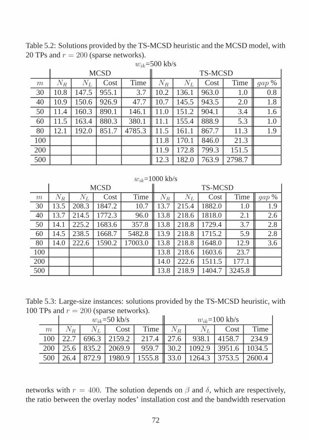
Table 5.2: Solutions provided by the TS-MCSD heuristic and the MCSD model, with20 TPs and r = 200 (sparse networks).

wik=500 kb/sMCSD TS-MCSD

m NR NL Cost Time NR NL Cost Time gap %30 10.8 147.5 955.1 3.7 10.2 136.1 963.0 1.0 0.840 10.9 150.6 926.9 47.7 10.7 145.5 943.5 2.0 1.850 11.4 160.3 890.1 146.1 11.0 151.2 904.1 3.4 1.660 11.5 163.4 880.3 380.1 11.1 155.4 888.9 5.3 1.080 12.1 192.0 851.7 4785.3 11.5 161.1 867.7 11.3 1.9

100 11.8 170.1 846.0 21.3200 11.9 172.8 799.3 151.5500 12.3 182.0 763.9 2798.7

wik=1000 kb/sMCSD TS-MCSD

m NR NL Cost Time NR NL Cost Time gap %30 13.5 208.3 1847.2 10.7 13.7 215.4 1882.0 1.0 1.940 13.7 214.5 1772.3 96.0 13.8 218.6 1818.0 2.1 2.650 14.1 225.2 1683.6 357.8 13.8 218.8 1729.4 3.7 2.860 14.5 238.5 1668.7 5482.8 13.9 218.8 1715.2 5.9 2.880 14.0 222.6 1590.2 17003.0 13.8 218.8 1648.0 12.9 3.6

100 13.8 218.6 1603.6 23.7200 14.0 222.6 1511.5 177.1500 13.8 218.9 1404.7 3245.8

Table 5.3: Large-size instances: solutions provided by the TS-MCSD heuristic, with100 TPs and r = 200 (sparse networks).

wik=50 kb/s wik=100 kb/sm NR NL Cost Time NR NL Cost Time

100 22.7 696.3 2159.2 217.4 27.6 938.1 4158.7 234.9200 25.6 835.2 2069.9 959.7 30.2 1092.9 3951.6 1034.5500 26.4 872.9 1980.9 1555.8 33.0 1264.3 3753.5 2600.4

networks with r = 400. The solution depends on β and δ, which are respectively,the ratio between the overlay nodes’ installation cost and the bandwidth reservation

72

Table 5.4: Large-size instances: solutions provided by the TS-MCSD heuristic, with100 TPs and r = 400 (dense networks).

wik=50 kb/s wik=100 kb/sm NR NL Cost Time NR NL Cost Time

100 20.5 600.9 2142.6 210.6 27.1 908.8 4145.2 260.1200 22.2 678.3 2065.1 933.4 29.8 1066.6 3933.8 1180.0500 24.8 799.2 1969.0 2144.7 32.1 1207.4 3748.5 2452.4

Table 5.5: Power Law topologies: solutions provided by the TS-MCSD heuristic inthe topologies with node degree power laws generated using BRITE, with 500 CSsand 20 TPs.

wik (kb/s) NR NL Cost Time500 4.0 52.0 823.6 1297.7

1000 10.0 130.0 2914.9 2493.4

cost, and the ratio between the cost of a link connecting two CSs which belong todifferent ISPs and that of a link connecting two CSs belonging to the same ISP.

The results obtained varying, respectively, the ratios β and δ are summarized inTables 5.6 and 5.7, and they are in line with those reported in Section 4.3 (e). Morein detail, it can be observed that (1) if β decreases, TS-MCSD tends to deploy moreoverlay nodes and (2) when δ increases, TS-MCSD tends to install less overlay nodesand links, thus diminishing the number of longer (and costlier) links that traversedifferent ISPs in the planned SON.

Table 5.6: Variable cost ratio β: solutions provided by the TS-MCSD heuristic with100 TPs, 100 CSs, wik=50 kb/s and r = 400 (dense networks).

β NR NL Cost Time10 20.5 600.9 2159.2 210.65 26.8 896.9 2041.5 233.81 33.9 1325.5 1914.6 255.4

1/10 36.3 1494.6 1880.0 256.4

73

Table 5.7: Variable cost ratio δ: solutions provided by the TS-MCSD heuristic with100 TPs, 100 CSs, wik=50 kb/s and r = 400 (dense networks).

δ NR NL Cost Time1 20.5 600.9 2159.2 210.62 14.2 390.9 3032.4 177.55 12.3 340.0 4870.0 179.0

10 11.7 326.1 7400.8 186.8

d) Real ISP Topologies

Finally, we considered three diverse ISP topologies which have been provided byTelecom Italia Lab (TILab). Table 5.8 lists, for each topology, the number of testpoints (n) and candidate sites (m), the overlay node installation cost (cI

j ) and capacity(Γj). All candidate sites have the same installation cost and the same capacity. Thetraffic demands, the access/egress costs and the transport costs are those provided byTILab for each network instance.

Table 5.9 shows the results obtained using the TS-MCSD heuristic on the TILabnetwork instances. Note that in all such real scenarios the proposed heuristic solvedthe MCSD problem with almost negligible computing time, thus representing a prac-tical solution for the planning of SONs.

Table 5.8: TILab Network instances: number of test points and candidate sites, over-lay node installation cost and capacity.

Network n m cIj Γj

TILab1 15 12 20 2000TILab2 39 17 100 500TILab3 49 49 60000 10000

We then derived other instances by reducing the overlay nodes capacities by afactor of 0.6 and 0.8, and by reducing the installation costs by a factor of 0.1, 0.01 and0.001. Tables 5.10 and 5.11 show the numerical results obtained in the three TILabtopologies with, respectively, the overlay node capacity reduction of 0.6 and 0.8, andthe installation cost reduction of 0.1, 0.01 and 0.001. For comparison reasons, inthese Tables we also reported the numerical results obtained without applying anyreduction factor (which are those already shown in Table 5.9).

74

Table 5.9: TILab topologies: solutions provided by the TS-MCSD heuristic.

Network NR NL Cost TimeTILab1 3.0 36.0 6412.3 0.1TILab2 4.0 90.0 13612.9 0.8TILab3 7.0 140.0 46590955.4 11.1

When the overlay nodes capacity decreases, the heuristic is forced to install moreoverlay nodes, and the total SON cost increases (see Table 5.10). On the other hand,when the overlay nodes installation cost decreases, TS-MCSD tends to install moreoverlay nodes (see Table 5.11, network topology TILab2), and the overall networkcost decreases. Finally, note that also for such network instances the computing timeof our proposed heuristic is very short.

Table 5.10: TILab topologies: solutions provided by the TS-MCSD heuristic. Anoverlay node capacity reduction of 0.6 and 0.8 has been applied. For comparisonreasons, the results obtained without capacity reduction (i.e., capacity reduction fac-tor = 1) are also reported.

Network Cap. Reduction Factor NR NL Cost TimeTILab1 0.6 4.0 42.0 7261.1 0.2TILab1 0.8 3.0 36.0 6538.3 0.2TILab1 1 3.0 36.0 6412.3 0.1

TILab2 0.6 5.0 98.0 13691.9 1.0TILab2 0.8 5.0 98.0 13691.9 1.1TILab2 1 4.0 90.0 13612.9 0.8

TILab3 0.6 10.0 188.0 49374604.8 11.5TILab3 0.8 8.0 154.0 47310633.0 13.2TILab3 1 7.0 140.0 46590955.4 11.1

75

Table 5.11: TILab topologies: solutions provided by the TS-MCSD heuristic. Theoverlay nodes installation costs have been reduced by a factor of 0.1, 0.01 and 0.001.For comparison reasons, the results obtained without cost reduction (i.e., cost reduc-tion factor = 1) are also reported.

Network Cost Reduction Factor NR NL Cost TimeTILab1 1 3.0 36.0 6412.3 0.1TILab1 0.1 3.0 36.0 6358.3 0.2TILab1 0.01 3.0 36.0 6352.9 0.2TILab1 0.001 3.0 36.0 6352.3 0.2

TILab2 1 4.0 90.0 13612.9 0.8TILab2 0.1 10.0 168.0 13057.0 1.0TILab2 0.01 10.0 168.0 12967.0 1.0TILab2 0.001 10.0 168.0 12958.0 1.0

TILab3 1 7.0 140.0 46590955.4 11.1TILab3 0.1 7.0 140.0 46241653.3 12.1TILab3 0.01 7.0 140.0 46203853.3 12.1TILab3 0.001 7.0 140.0 46200073.3 12.1

76

Chapter 6

Introduction to Game Theory

In this chapter we give a short introduction to Algorithmic Game Theory in orderto provide the reader with the fundamental framework for understanding the nextChapter. A more extensive discussion can be found in [57].

6.1 Strategic Games

There are a lot of situations occurring in real life in which we seek for the maximiza-tion of our own benefit and very often the final outcome of our efforts also dependson the behavior of other people we have no control on. This is what is usually calleda strategic game.

Definition 1 A strategic game G consists of a set I of k ≥ 2 players, where eachplayer i ∈ I has a (finite) set of strategies Si and a payoff function J i: S1×. . .×Sk →R+, for 1 ≤ i ≤ k.

One of the most famous strategic games is the Prisoner’s Dilemma that we recallin the sequel for the sake of completeness.

EXAMPLE (Prisoner’s Dilemma)

Two suspects in a major crime are held in separate cells. There is enough evidenceto convict each of them of a minor offense, but not enough evidence to convict eitherof them of the major crime unless one of them acts as an informer against the other(finks). If they both stay quiet, each will be convicted of the minor offense and spendone year in prison. If one and only one of them finks, he will be freed and used as awitness against the other, who will spend four years in prison. If they both fink, each

77

will spend three years in prison. This situation can be modeled as a strategic game inwhich we have two players 1 and 2. The set of strategies is the same for both of themand is Si = {Quiet, F ink}, for i ∈ {1, 2}. Finally, the payoff function is depictedin Table 6.1, in which the rows represent the first player strategies and the columnsthe second player ones.

Table 6.1: The Prisoner’s Dilemma.Quiet Fink

Quiet (2,2) (0,3)Fink (3,0) (1,1)

Once defined a particular strategic game, the next step is that of characterizingthe players’ behavior. In other words, we have to determine which strategy will bechosen by each player in the game. Before settling out this question, it is necessaryto fix some important points about the players’ nature and how powerful is theirdecision-making process. The classical assumption is that each player acts rationallyand selfishly, that is, he tries to maximize his own payoff and is not interested incooperating with other players unless this can improve his payoff. It is also usuallyassumed that a player knows the strategy chosen by all the other players at any time.

Definition 2 Given a game G, a state s of G is an assignment of a strategy to eachplayer. More formally, s is an element of the set S = S1 × . . . × Sk.

The outcome of a strategic game is usually defined as a stable state, that is a statein which all players are satisfied with their payoff so that none of them is willing tochange his chosen strategy.

6.2 Dominant Strategies

In any game, a player’s strategy strictly dominates another strategy if it is superior,no matter what the other players do.

Definition 3 In a strategic game with k players, we say that player i’s strategysi ∈ Si strictly dominates his strategy s′

i ∈ Si, if J i(s1, . . . , si, . . . , sk) ≥J i(s1, . . . , s

′i, . . . , sk), for every strategy sj ∈ Sj adopted by any other player j ∈

{1, . . . , k}, j �= i. A dominant strategy for player i is a strategy si ∈ Si that strictlydominates any other strategy s′i ∈ Si.

78

In the Prisoner’s Dilemma, for example, the strategy Fink strictly dominates thestrategy Quiet; regardless of his opponent’s strategy, a player prefers the outcomewhen he chooses Fink to the outcome when he chooses Quiet. Since there are onlytwo strategies, it follows that Fink is a dominant strategy. Clearly, because of hisrational behavior, a player will always adopt a dominant strategy each time he hasan available one. Thus, if each player has a dominant strategy, the outcome of thegame will be the stable state in which each player adopts his dominant strategy. Inparticular, for the Prisoner’s Dilemma the outcome will be s = {Fink, F ink}. Inthe sequel, we will call each such a state s, a Dominant Strategies Equilibrium.

6.3 Nash Equilibrium

The use of dominant strategies in order to characterize the outcome of a strategicgame is perfectly reasonable and appropriate. The problem is that the existence of adominant strategy for each player is a very strong property and the majority of thegames we can think of does not satisfy it.

Starting from this point, John Nash in his Ph.D. thesis [58] elaborated his char-acterization of stable state in a strategic game by introducing his famous concept ofequilibrium point.

Definition 4 A state s = (s1, . . . , si, . . . , sk) is a Nash Equilibrium (NE) if for everyplayer i and strategy s′i ∈ Si it holds thatJ i(s1, . . . , si, . . . , sk) ≥ J i(s1, . . . , s

′i, . . . , sk).

It can soon be noted the similarity of this definition with the one of dominantstrategies. In effects, the strategy adopted by a player in any NE is a dominant strat-egy once fixed the strategy adopted by any other player. Hence, Nash introduced aweaker but still reasonable form of dominance thus making his notion of equilibriummore practical (in the sense that we can expect games not having a Dominant Strate-gies Equilibrium to possess a NE), but clearly not immune from criticisms. The firstof them is that a NE is a stable state of a game as soon as we consider non-cooperativegames, that is games in which no coalitions of players can be formed. In fact, thedominance condition required in a NE only involves one player at time, but nothingis said when two or more players jointly decide to choose a different strategy. An-other important fact is that a game can admit more than just a single NE thus arisingthe problem of discriminating among them.

Finally, the adoption of NE as model of behavior does not settle out definitivelythe problem of determining the outcome of a strategic non-cooperative game sinceeven existence of NE cannot be guaranteed in any game.

79

6.4 Algorithmic Game Theory

A very novel and fascinating research area is developing from the intersection ofGame Theory with Theoretical Computer Science. In Christos Papadimitriou’s words:“If the second half of the Twentieth Century has been devoted to the understanding ofthe power of the von Neumann’s machine as a computational model, in the next yearsone of the major goals of our community will be that of providing a good mathemat-ical formulation, understanding and analysis of the new millennium’s computationalmodel: the Internet”. The main implication coming from this assumption is that nowthe way in which the classical optimization problems on networks can be addressedand solved has to be heavily reviewed. In non-cooperative networks, in fact, it isusually the case that the variables defining a given combinatorial problem are therepresentation of independent agents that may not be willing to implement the (op-timal, approximate or competitive) solution computed with the classical techniques,for several reasons. It is well known that the lack of cooperation among the playersin a game may result in suboptimal situations. To explain how we can define andmeasure the quality of a stable state, let us recall the Prisoner’s Dilemma game. Inthe only stable state of the game (no matter if we use Dominant Strategies Equilibriaor NE for its definition), s = {Fink, F ink}, both players get a payoff equal to 1,while if they cooperate to agree on the state s′ = {Quiet, Quiet} the payoff wouldbe equal to 2 for both of them. This is a classical example showing that stable statesfail in optimizing the social outcome of a game, where the social outcome of a gameis defined here as the sum of the players’payoffs, but can be represented by any func-tion f : S → R+ defined over the set of states of the game and not necessarily relatedto the players’ payoffs.

In practice, this means that the selfish behavior of the agents populating a non-cooperative system can result in a stable state whose social value may be far fromthe social optimum, thus resulting in an unbearable degradation of the system’s per-formances. There are several approaches that has been developed in order to copewith the selfish behavior of the players in a game so as to keep the social outcomewithin some acceptable bounds, or simply to force players to act fairly and coop-eratively while preserving their independence. All these techniques aim to designsimple games so as their outcome will result in the desired one.

In spite of some of its faults, the classical theory of NE has been accepted and ex-ploited worldwide to model the stable outcome of strategic games in non-cooperativenetworks and, at the same time, is being enriched with the notions of computationalcomplexity and efficiency. Thus, in the main approaches followed in the literature byboth Economists and Computer Scientists, stable states are usually modeled as NE.In what follows we give a brief overview of the main challenges posed by the study

80

of NE in non-cooperative strategic games.

6.4.1 Existence of Nash Equilibria

It is not difficult to convince oneself that the first concern one has to due with whenapproaching a non-cooperative strategic game is to prove that it admits at least oneNE. In fact, if the game we are facing does not possess this basic property, no stablestate can be reached by the players and so no further study on such a game can beconsidered plausible.

6.4.2 Computing Nash Equilibria

One of the fundamental aspects of NE is that they are stable states which can bereached by players independently by simply performing improving steps. But whatabout the problem of computing a NE? This is a very interesting computational prob-lem since its complexity is still astonishingly open. On the other hand, if we are in-teresting in computing extreme NE, that is NE minimizing or maximizing the socialfunction, they can be usually proved to be NP-hard to compute. In the case of ourinterest of computing NE, we observe that, if convergence is proved through a po-tential function Φ, then Φ can be used to implement an algorithm determining a NEby repeatedly computing for any state s ∈ S, the state s′ ∈ S such that Φ(s) −Φ(s′)is maximized. Unfortunately, such an algorithm cannot achieve in general a polyno-mial running time. For an interesting analysis on the complexity of determining NE,see [59]. It is also worth noting that, when the social function f we want to optimizeis defined as the sum of all players’ payoffs, any NE corresponds to a local optimumfor the optimization problem having S as set of feasible solutions and f as objectivefunction, and viceversa. Thus any NE can be seen as the solution returned by a localsearch algorithm defined by a 1-neighborhood function and the price of anarchy ofthe game becomes the approximation ratio of such an algorithm.

6.4.3 Bounding the prices of Anarchy and Stability

Once we know that a game possesses a NE an intriguing issue is that of determiningthe quality of a NE. In order to measure the loss of optimality that an unregulatedsystem has to suffer because of the lack of coordination of his agents with respectto some social function, Koutsoupias and Papadimitriou [21] introduced the notionof price of anarchy of a game as the supremum over all NE of the ratio between thesocial value of a NE and the social optimal. More formally,

81

Definition 5 Given a game G and a social function f , let N be the set of all NE ofG and OPT be a state of G optimizing f . The price of anarchy PoAG(f) of game Gaccording to f is defined as

PoAG(f) = sups∈N

f(s)

f(OPT )

The price of anarchy is defined as a worst case evaluation of the social value of aNE.

In [14] the term price of stability has been introduced as the ratio between thebest NE and the social optimum.

Definition 6 Given a game G and a social function f , let N be the set of all NE ofG and OPT be a state of G optimizing f . The price of stability PoSG(f) of game Gaccording to f is defined as

PoSG(f) = infs∈N

f(s)

f(OPT )

This notion measures the minimum loss in optimality that an unregulated systemhas to suffer. Its importance is strictly related to the problem of computing NE.

In fact, if it is possible to compute the best NE, say s ∈ S, in polynomial time,we can imagine a scenario in which a trusted authority suggests an initial choice toeach player when entering the game so that the resulting state is exactly s. No playerwill have an improving step and so the loss in optimality will be exactly equal to theprice of stability, that is the minimum possible one.

82

Chapter 7

Socially-Aware Overlay NetworkDesign Games

In many scenarios, network design is not enforced by a central authority, but arisesfrom the interactions of several self-interested agents. This is the case of the Inter-net, where connectivity is due to Autonomous Systems’ choices, but also of overlaynetworks, where each user client can decide the set of connections to establish.

Recent works have used game theory, and in particular the concept of Nash Equi-librium, to characterize stable networks created by a set of selfish agents. The major-ity of these works assume that users are completely non-cooperative, leading, in mostcases, to inefficient equilibria. However, this assumption is not entirely realistic, forexample when network design involves long-term decisions. Moreover, incentivescould be introduced by some external authority (e.g., the overlay administrator) inorder to increase the users’ cooperation level.

This Chapter overcomes this limitation by first proposing a novel network for-mation game, the Socially-Aware Network Design game, where users are partiallysocially-aware because their utility function is a weighted sum of individual andglobal costs. We study the efficiency of the equilibria achieved by our game, deriv-ing bounds to the Price of Anarchy, the Price of Stability and the Reachable Price ofAnarchy. These results suggest that the more sensitive users are to the global cost,the more efficient the best stable network is. However, we show that highly socially-aware users can also design networks much more expensive than purely selfish users.

For this reason, to eliminate worst-case scenarios while enabling at the same timemore efficient Nash equilibria, we further propose a Stackelberg (leader-follower) ap-proach, where a leader (e.g., the overlay network administrator) architects the desirednetwork buying an appropriate subset of network’s links, driving in this way the usersto overall efficient Nash equilibria.

83

Finally, we measure the performance of the proposed schemes in several networkscenarios, including realistic topologies where players build an overlay on top of realInternet Service Provider networks.

The Chapter is organized as follows: Section 7.1 introduces the proposed Socially-Aware Network Design game. Section 7.2 proposes a greedy algorithm that imple-ments best response dynamics, which permits to reach a Nash equilibrium in the pro-posed game. Section 7.3 provides precise bounds on the Price of Anarchy, the Priceof Stability and the Reachable Price of Anarchy for the SAND game. Section 7.4describes the proposed Stackelberg game (the Network Administrator-Driven SANDgame), which enables very efficient Nash equilibria. Finally, Section 7.5 presentsnumerical results that demonstrate the effectiveness of the SAND and NAD-SANDgames in several realistic network scenarios.

7.1 The Socially-Aware Network Design Game

This Section illustrates the proposed Socially-Aware Network Design (SAND) game,motivating the reason to introduce such model.

The SAND game occurs in a directed graph G = (V, E), where each edge e has anonnegative cost ce, and each player i ∈ I = {1, 2, . . . k} is identified with a source-sink pair (si, ti). Every player i picks a path Si from its source to its destination,thereby creating the network (V,∪iSi) with total cost equal to

∑e∈∪iSi

ce, which willbe referred to as social cost. We will refer to the path Si also as the strategy chosenby player i.

This social cost is assumed to be shared among the players in the following way:let xe denote the number of overlay paths that go through overlay link e; if edge e liesin xe of the chosen paths, then each player choosing such an edge pays a proportionalshare πe = ce

xeof the cost.

The objective function J i that user i wants to minimize is therefore given by:

J i =∑e∈Si

πe + α∑

e∈∪jSj

ce (7.1)

The first term takes into account the selfish nature of each player, since it is thecost for user i to buy the edges belonging to the chosen path, Si; on the other hand,the second term represents the total network cost (i.e., the social cost), α being aparameter that permits to give more weight to one component with respect to theother.

An alternative interpretation of objective function (7.1) is also possible: we canthink that users are completely selfish, but the social-aware term in cost function (7.1),

84

α∑

e∈∪jSjce, is imposed by the network operator. The advantage of such approach

is that the operator does not need to solve a large-scale Integer Linear Programmingproblem in order to optimize the routing choices for every change in the network(either in the topology, links cost, players location etc . . . ), but can let the users solvethe problem in a distributed way, converging to a good and stable solution.

Note that for α = 0 objective function (7.1) corresponds to that of the Shapleynetwork design game proposed in [14], which represents a particular case of ourproposed game. Furthermore, in our game, users need only a limited amount ofinformation, which is exactly equal to that of the Shapley network design game.

The SAND game belongs to the class of potential games, which has been iden-tified in [60]. Such games are characterized by a real-valued function, Φ, on thestrategy vector (S) which measures exactly the difference in the cost that any playersaves if he is the only player to deviate. Mathematically, if we define:

• S = (S1, S2, . . . , Sk) the vector of players’ strategies,

• S ′i �= Si an alternate strategy for some player i,

• S−i the strategy played by all other players than i, and

• S ′ = (S ′i, S−i),

then a potential game with k players is characterized by a potential function, Φ(S),such that for any user i we have Φ(S) − Φ(S ′) = J i(S) − J i(S ′).

Potential games have nice properties, such as existence of at least one pure Nashequilibrium, namely the strategy S that minimizes Φ(S) [57]. Furthermore, in suchgames, best response dynamics always converge to a Nash equilibrium.

It is easy to verify that the SAND game is characterized by the following potentialfunction:

Φ(S) =∑e∈E

xe∑x=1

ce

x+ α

∑e∈∪jSj

ce. (7.2)

We observe that the SAND game is a potential game without being at the sametime a congestion game on the given graph G [61]. In fact, the cost incurred by playeri, J i, is not simply the sum of the costs incurred by such player from each link in thechosen path Si, but it includes a further term, the total network cost (multiplied bythe parameter α.)

Since we have introduced a term proportional to the network cost in the objectivefunction of each player, we expect that players should design better networks, eventhough Section 7.3 shows that this is not necessarily the case. Before addressing this

85

issue, we present in the following Section a possible asynchronous users operationthat implements best response dynamics and hence converges to a Nash equilibrium.

Comments

The SAND game can be easily extended to take into account performance metricscommonly used in routing problems in communication networks. For example, wecan imagine that users are sensitive not only to link costs but also to the allocatedrate on each link e, which we can assume is inversely proportional to the number ofusers (xe) that pass through such link (like in congestion games [61]).

The extension can be performed adding a third term (a congestion cost) to costfunction (7.1), which becomes as follows:

J i =∑e∈Si

πe + α∑

e∈∪jSj

ce + γ∑e∈Si

xe

re

(7.3)

where re is the maximum transmission rate of link e (i.e., the link’s capacity), andγ is a weight that expresses the user’s sensitivity to congestion costs. The rationaleof adding γ

∑e∈Si

xe

reto the cost function is that the congestion cost of using link e

increases with the number of players that choose such link, since the allocated rate( re

xe) decreases accordingly.The extended SAND game is still a potential game, with the following potential

function:

Φ(S) =∑e∈E

xe∑x=1

(ce

x+ γ

x

re

)+ α

∑e∈∪jSj

ce. (7.4)

Therefore, the existence of pure Nash equilibria is guaranteed, as well as the conver-gence of best response dynamics.

Finally, we note that the best response algorithm illustrated in the next Sectioncan be extended straightforwardly to take into account the newly added congestioncost.

7.2 Best Response Algorithm

We now describe a simple algorithm that implements best response dynamics, al-lowing each user to improve its cost function in the proposed SAND game. Suchalgorithm, detailed in the following, is the best response strategy for a user minimiz-ing objective function (7.1), assuming other users are not changing their strategies.

86

We still consider a directed graph G = (V, E), where each edge e has a nonneg-ative cost ce.

Let us consider a vector of players’ strategies S = (S1, S2 . . . Sk), where Si ⊂ Eis a set of edges that connect the source-sink pair (si, ti). Let us denote by S−i =∪j �=iSj the set of edges used by all players except player i; as a consequence, the setE −S−i contains all links that are not used by the set of all players except i. Finally,let ke denote the number of times that edge e lies in the paths chosen by such players(i.e., all players except player i).

Algorithm 4 allows user i to determine the best response to all other users’ strate-gies. The rationale behind such algorithm is very simple: the link weights are setequal to the cost incurred by user i to choose them, according to objective func-tion (7.1). Then, the shortest path corresponds to the choice that minimizes the user’scost, and it represents therefore its best response. Note that, if multiple shortest pathsexist with the same cost, the player chooses one of them randomly.

Algorithm 4 Pseudo-code specification for the best response dynamics for the SANDgame.

1: if e ∈ S−i then2: Set Cost(e) = ce

ke+1

3: else4: Set Cost(e) = ce · (1 + α)5: end if6: Compute the least-cost path (using for example the Dijkstra algorithm) with link

costs Cost(e)7: Set Si equal to the set of links contained in the least-cost path

7.3 Bounds on the Price of Anarchy, Price of Stabil-ity and Reachable Price of Anarchy for the SANDgame

In this Section, we derive bounds on the Price of Anarchy (PoA), the Price of Sta-bility (PoS) and the so-called Reachable Price of Anarchy (RPoA) for the Socially-Aware Network Design game, and compare them with the results presented in [14]for the Shapley Network Design game. This allows us to determine the worst andbest case performance of our proposed game.

87

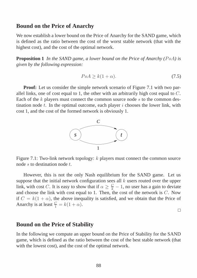
Bound on the Price of Anarchy

We now establish a lower bound on the Price of Anarchy for the SAND game, whichis defined as the ratio between the cost of the worst stable network (that with thehighest cost), and the cost of the optimal network.

Proposition 1 In the SAND game, a lower bound on the Price of Anarchy (PoA) isgiven by the following expression:

PoA ≥ k(1 + α). (7.5)

Proof: Let us consider the simple network scenario of Figure 7.1 with two par-allel links, one of cost equal to 1, the other with an arbitrarily high cost equal to C.Each of the k players must connect the common source node s to the common des-tination node t. In the optimal outcome, each player i chooses the lower link, withcost 1, and the cost of the formed network is obviously 1.

ts

1

C

Figure 7.1: Two-link network topology: k players must connect the common sourcenode s to destination node t.

However, this is not the only Nash equilibrium for the SAND game. Let ussuppose that the initial network configuration sees all k users routed over the upperlink, with cost C. It is easy to show that if α ≥ C

k− 1, no user has a gain to deviate

and choose the link with cost equal to 1. Then, the cost of the network is C. Nowif C = k(1 + α), the above inequality is satisfied, and we obtain that the Price ofAnarchy is at least C

1= k(1 + α).

�

Bound on the Price of Stability

In the following we compute an upper bound on the Price of Stability for the SANDgame, which is defined as the ratio between the cost of the best stable network (thatwith the lowest cost), and the cost of the optimal network.

88

Proposition 2 In the SAND game, the Price of Stability (PoS) is upper bounded bythe following expression:

PoS ≤ Hk + α

1 + α. (7.6)

Proof: It is shown in [14, 57] that the function Ψ(S) =∑

e∈E

∑xe

x=1ce

xis an

exact potential function for the Shapley network design game revised in Section 2.2,page 11. Furthermore, it is shown in [57] that such function satisfies the followinginequalities:

cost(S) ≤ Ψ(S) ≤ Hkcost(S) (7.7)

where cost(S) =∑

e∈∪jSjce and Hk =

∑ki=1 1/i is the kth harmonic number.

The potential function of the SAND game, Φ(S), is directly related to that of theShapley network design game, Ψ(S). In fact, from expression (7.2) it can be easilyseen that Φ(S) = Ψ(S)+α·cost(S). Hence, if we replace Ψ(S) = Φ(S)−α·cost(S)in expression (7.7), it follows that:

(1 + α)cost(S) ≤ Φ(S) ≤ (Hk + α)cost(S). (7.8)

Finally, Theorem 19.13 in [57] states that if a potential game with potential func-tion Φ(S) satisfies the following inequality:

cost(S)

A≤ Φ(S) ≤ Bcost(S) (7.9)

with A and B positive constants, then the Price of Stability (PoS) is at most AB.Therefore, in our problem, we obtain that the Price of Stability is at most Hk+α

1+α.�

Bound on the Reachable Price of Anarchy

We now derive a bound on the so-called Reachable Price of Anarchy (RPoA), aquantity defined in [19]. The denominator of this ratio is the cost of the sociallyoptimal network, which we denote by C opt; the numerator is the largest cost of anequilibrium reachable via the following process: the k players enter the game one-by-one in an arbitrary order, and each picks a path of minimum cost (according toobjective function (7.1)), given the choices of previous players. After all playershave entered, the game proceeds exactly as for the SAND game, with each player re-optimizing its path, given the current strategies of all other players (using for example

89

the best response algorithm illustrated in the previous Section). When the processreaches a Nash equilibrium (as it must, since it is a potential game), it stops.

Proposition 3 In the SAND game, the Reachable Price of Anarchy (RPoA) is upperbounded by the following expression:

RPoA < kα + 1

α + 1k

. (7.10)

Proof: Let Sopti define the path from source node si to destination node ti for

player i in the optimal outcome (the least cost network), and let Si denote the pathchosen by player i in its first move in the game. Let C(Sopt

i ) =∑

e∈Sopti

ce and

C(Si) =∑

e∈Sice denote the costs of such two paths.

For the first player that enters the network, the following inequality holds:∑e∈S1

πe + α∑e∈S1

ce = (1 + α)C(S1) < (1 + α)C(Sopt1 ).

For the second player, the following inequality holds:∑e∈S2

πe + αC(S1 ∪ S2) <∑

e∈Sopt2

πe + αC(S1 ∪ Sopt2 )

which can also be expressed as follows, observing that C(S1 ∪ Sopt2 ) < C(S1) +

C(Sopt2 ), and that

∑e∈Sopt

2πe ≤ C(Sopt

2 )∑e∈S2

πe + αC(S1 ∪ S2) < (1 + α)C(Sopt2 ) + αC(Sopt

1 ).

It can be further observed that: ∑e∈Si

πe ≥ 1

kC(Si),

since in the best outcome, each of the links belonging to the path chosen by player iis shared by all k players.

If we proceed iteratively, we finally obtain the following inequality:

(α +1

k)C(

k⋃i=1

Si) < (1 + α)

k∑i=1

C(Sopti )

which can be rewritten as follows, observing that∑k

i=1 C(Sopti ) ≤ kCopt :

90

(α +1

k)C(

k⋃i=1

Si) < (1 + α)kCopt.

This allows us to obtain the following result:

C(⋃k

i=1 Si)

Copt< k

α + 1

α + 1k

. (7.11)

Hence, the cost of the network reached after the first move of each of the k play-ers, C(

⋃ki=1 Si), is no more than k α+1

α+ 1k

times the optimal cost, C opt. Since subsequent

best response moves performed by players decrease the potential function value Φ(S)given by expression (7.2) (simulating a local search on it), the players will convergeto a Nash equilibrium whose cost is still within k α+1

α+ 1k

times the optimum.

Therefore, we can conclude that the Reachable Price of Anarchy is at most k α+1α+ 1

k

.

�

Comments

For α = 0 the SAND game is equivalent to the original Shapley network designgame. Indeed, expressions (7.5) and (7.6) confirm the results already demonstratedin [14]: PoA = k and PoS = Hk. In the SAND game, for increasing α values, theupper bound on the PoS decreases, and tends to 1 for α → ∞ (then also PoS → 1).This can be easily explained since for α → ∞ the social component of objectivefunction (7.1) is predominant. In this limiting behavior, all users share the sameutility function, which is the second term of expression (7.1); in such a situation, thesocial network optimum (i.e., the network with the minimum total cost) is obviouslyalso a Nash equilibrium, since the objective function of each single player coincideswith the social network cost (multiplied by α).

On the other hand, our lower bound on the PoA increases when α increases. Thiscorresponds to the (quite counter-intuitive) fact that, in some cases, more socially-aware users can design less efficient networks. This happens for example in thesimple instance of Figure 7.1. Such inefficiency is due to the myopic decision cri-terion: each player only considers the effect of its own choice (i.e., changing theselected path), without considering eventual future decisions from the other players.

However, it can be observed from expression (7.10) that the RPoA of the SANDgame strictly decreases for increasing α values. For large α values (notably, forα → ∞), the RPoA is less than k. Therefore, if the SAND game is played starting

91

from an empty network, worst-case scenarios like that illustrated in Figure 7.1 areeliminated.

Finally, our simulations show that the Nash equilibria reached in the SAND gameare, in average, consistently better than those achieved by the Shapley game, as wewill show in Section 7.5.

7.4 The Network Administrator-Driven Socially-AwareNetwork Design game

We now illustrate a variation of the SAND game, named the Network Administrator-Driven SAND (NAD-SAND) game, where a network administrator plays before theusers, and his aim is to drive them to the best Nash equilibrium possible.

Since computing the optimal Stackelberg strategy is NP-hard, we present in thisChapter a simple strategy that achieves consistent performance improvements. Suchapproach is implemented via the following heuristic:

1. Given the network topology, the network administrator solves a generalizedSteiner Tree problem [62], determining the minimum-cost subnetwork suchthat the source/destination nodes of each player are connected by a path. LetEopt be the set of edges belonging to such optimal subnetwork.

2. The network administrator chooses all links belonging to E opt, thus offering toshare eventually their cost with the other players. Therefore, using the notationintroduced in Section 7.1, after this step we have xe = 1, ∀e ∈ Eopt (that is,the network administrator has already chosen all links that are optimal from asocial point of view).

3. At this point, all the k users play the SAND game, each trying to optimize itsown objective function, which is the same of expression (7.1).

The reader is referred to Appendix A.2 for a brief overview of the Steiner Treeproblems in networks.

The rationale behind the proposed NAD-SAND game is the following: the net-work administrator tries to motivate all players to use the links that belong to thesocially optimal solution by sharing their cost with network users. We will show inthe next Section that such heuristic is very effective, and permits to obtain dramaticperformance improvements with respect to the SAND game.

We observe that the first step of the NAD-SAND game involves solving an NP-Complete problem. However, several efficient heuristics and approximation algo-rithms have been proposed to solve such problem in a reasonable computation time [62,

92

63, 64]. In the numerical results presented in the next Section we were able to com-pute exactly the minimum cost generalized Steiner tree using a simple ILP formula-tion, and solving it with the CPLEX solver [47].

Finally, we observe that as α → ∞, the NAD-SAND game always reaches theminimum cost network since for each player the cost of choosing any link that doesnot belong to the minimum-cost subnetwork (i.e., to E opt) has an exceedingly largecost. As a consequence, PoA → 1 as α → ∞.

We now derive a lower bound on the Price of Anarchy for the NAD-SAND game.

Proposition 4 In the NAD-SAND game, a lower bound on the Price of Anarchy(PoA) is given by the following expression:

PoA ≥ k

2(1 + α)(7.12)

for α ≤ k2− 1.

Proof: Let us consider the network scenario illustrated in Figure 7.2, where eachof the k players must connect the source node si to the common destination node t.Link ν → t has a cost equal to C, with 2 ≤ C ≤ k.

The minimum cost generalized Steiner Tree is in this case formed by all linkssi → ν (with cost zero) and by link ν → t, so that its cost is equal to C. Hence, thenetwork administrator will choose all these links, which constitute the E opt set.

In the optimal outcome, each player i chooses the si → ν → t path, and the costof the formed network is C.

1 111 1

s1 s2 s3 sksk−1

0 0 0 0 0

. . . .

. . . .

. . . .

Cv

t

Figure 7.2: Parallel link topology: bound on the Price of Anarchy for the NAD-SAND game.

93

The NAD-SAND game, however, admits another Nash equilibrium. Let us sup-pose that initially all k users are routed over the direct path, si → t, with total cost k.It can be easily seen that if α ≤ C

2− 1, no user has a gain to deviate and choose the

si → ν → t path, with cost equal to C.Then, the cost of the network is k. Now if C = 2(1 + α), the above inequality is

satisfied, and we obtain that the Price of Anarchy is at least kC

= k2(1+α)

.�

7.5 Numerical Results

In this Section, we report the results obtained by the proposed Socially-Aware Net-work Design (SAND) and Network Administrator - Driven SAND (NAD-SAND)games in random network topologies as well as in real ISP topologies, comparingthem both to the Shapley network design game [14] and to the social optimum.To this end, we consider both randomly generated network instances and real ISPtopologies mapped by the Rocketfuel tool [40, 41]. Random networks are obtainedusing a custom generator as well as a degree-based generator (BRITE [44, 45]) tocreate topologies with a power law distribution of node degrees.

In all cases, we start from the empty network and we apply iteratively the bestresponse algorithm illustrated in Section 7.2, until a Nash equilibrium is reached.

For each scenario we report the total network cost obtained by the proposedgames for different α values, as well as the optimal network cost (the ILP column),obtained formulating the generalized Steiner Tree problem [62] with an Integer Lin-ear Program (ILP), using AMPL [46], and solving it with the CPLEX solver [47].Solving such problem provides the least-cost network topology that connects allsource/destination pairs, thus representing a term of comparison for the efficiencyof the equilibria reached by our proposed games.

Finally, we evaluated numerically the Price of Anarchy and the Price of Stabilityin all our simulation settings, and we found that they are, respectively, always lessthan 1.78 and 1.56, hence consistently lower than the bounds provided in Section 7.3.

Full-Mesh Topologies

We first consider full-mesh network topologies with 50 nodes randomly distributedon a 1000 × 1000 square area and 20 players (source/destination pairs). The cost ofeach link is equal to its length, and the numerical results, averaged over 20 randomextractions, are reported in Table 6.1.

The SAND game permits to obtain network equilibria with a cost significantly

94

lower (approximately 13%) than that obtained with the Shapley network design game(i.e., the SAND row with α = 0), even though there is still room for improvements,as demonstrated by the gap existing between the SAND game and the optimal cost(the ILP column).

This gap is filled by the NAD-SAND game, which achieves consistently cheaperNash equilibria for all α values (up to more than 30%), including the α = 0 case,thus representing a very effective approach also when applied to the original Shapleynetwork design game. Furthermore, when α is sufficiently large (≥ 10), the NAD-SAND game reaches exactly the optimum (i.e., the generalized Steiner Tree cost).

Table 7.1: Full-Mesh topology with 50 nodes randomly distributed on a 1000 ×1000 area and 20 players: average network costs for the SAND and the NAD-SANDgames. The optimal network cost is also reported. The cost of each link is set equalto its length.

Game α = 0 α = 1 α = 10 α = 50 α = 100 α = 1000 ILPSAND 6956.17 6124.62 6037.53 6043.82 6050.94 6046.66

4214.63NAD-SAND 5718.86 4707.48 4214.63 4214.63 4214.63 4214.63

Random Topologies

To generate random network instances, we have implemented a topology generatorwhich considers a square area with edge equal to 1000, and randomly extracts theposition of N nodes, uniformly distributed on the square area.

As for the network links, which can be bought by players to connect their end-points, we consider two alternative choices:

• Random geometric graphs: links exist between any two nodes located withina range R. The link cost is set equal to its length.

• Random network model “Uniform”: a given number of links, L, is generatedbetween randomly extracted couples of nodes. The cost of each link is uni-formly distributed in the 0 to C range (C being the maximum link cost).

Given a random network, 20 random selections of k = 20 source/destinationcouples are considered.

Figure 7.3 shows the networks resulting at the Nash equilibria with the SANDgame in a random geometric graph scenario with 50 nodes, range R = 500, 20source/destination pairs, and two different α values (viz., α = 0 and α = 50).

95

0 100 200 300 400 500 600 700 800 900 10000

100

200

300

400

500

600

700

800

900

1000

(a) α = 0

0 100 200 300 400 500 600 700 800 900 10000

100

200

300

400

500

600

700

800

900

1000

(b) α = 50

Figure 7.3: Nash equilibria obtained by the SAND game in a random geometricnetwork with 50 nodes, R = 500, 20 source/destination pairs, and different α values(α = 0 and α = 50).

We observe that for α = 50 the topology is much closer to a tree-like topologythan that obtained by the Shapley network design game (α = 0). This is reflected inthe total network cost, which is equal to 7046.3 for α = 0 and to 5336.2 for α = 50,thus resulting in a gain of more than 24%.

Table 6.2 illustrates the results obtained in the same random network scenario ofFigure 7.3, with 50 nodes, range R = 500 and 20 source/destination pairs (players).The results are averaged on 20 source/destination random selections, and also on 5

96

random topologies. The Table reports the total cost of the network planned by theSAND and NAD-SAND games, as well as the optimal network cost. Also in thisscenario, the SAND game achieves improved equilibria with respect to the Shapleynetwork design game (up to 13.2%). The NAD-SAND game outperforms the SANDgame, further decreasing the planned network cost, and reaches, for α ≥ 10, thesocial optimum.

Table 7.2: Random geometric graphs; random networks with 50 nodes, R = 500 and20 players: average network costs for the SAND and the NAD-SAND games. Theoptimal network cost is also reported.


4213.82NAD-SAND 5645.44 4675.13 4213.82 4213.82 4213.82 4213.82

Table 6.3 shows the numerical results obtained using Random network model“Uniform” in networks with 100 nodes, L = 2000 links, maximum link cost C = 100and 20 source/destination pairs. The total network costs are illustrated in the Table forboth the SAND and NAD-SAND games, while the ILP column reports the optimalnetwork cost. Although there is still room for improvement, in this scenario theSAND game approaches the ILP bound, and consistently improves the quality ofnetwork equilibria with respect to the α = 0 case.

Also in this case, the NAD-SAND game performs better than the SAND game,lowering the overall network cost of more than 11%, reaching the socially optimaloutcome for α ≥ 50.

Table 7.3: Random network model “Uniform”; random networks with 100 nodes,2000 links, maximum link cost C = 100, 20 players: average network costs for theSAND and the NAD-SAND games. The optimal network cost is also reported.


263.25NAD-SAND 295.85 274.38 263.70 263.25 263.25 263.25

Power Law topologies

We further considered BRITE, a degree-based topology generator, which was usedto generate power law topologies; the Barabasi − Albert model was adopted withdefault parameters provided by BRITE.

97

We generated two different power-law network scenarios: one with 100 nodesand average node degree equal to 3, which contained about 300 links; the other with300 nodes and average node degree equal to 5, which contained about 1500 links.The cost of each link was set equal to its length.

Table 6.4 reports the corresponding numerical results, including the optimal net-work cost obtained solving the ILP model.

In this case, the Nash equilibria reached by the Shapley network design gameare already close to the optimum. This is mainly due to the fact that power lawtopologies, which result in short characteristic path lengths and heavy clustering, arethe result of social concerns that eventually bring efficiency to the network design(even though not explicitly expressed in the underlying routing protocols design).

The SAND and NAD-SAND games, however, permit to improve the efficiencyof such equilibria, finally obtaining the minimum cost network provided by the ILPmodel.

Table 7.4: Power law topologies generated using BRITE: average network costs forthe SAND and the NAD-SAND games. The optimal network cost is also reported.

100 nodesGame α = 0 α = 1 α = 10 α = 50 α = 100 α = 1000 ILPSAND 15980.20 15684.28 15596.31 15593.69 15593.43 15602.21

15314.14NAD-SAND 15479.98 15314.14 15314.14 15314.14 15314.14 15314.14

300 nodesGame α = 0 α = 1 α = 10 α = 50 α = 100 α = 1000 ILPSAND 22580.82 22312.27 22224.65 22210.97 22210.55 22210.55

21927.41NAD-SAND 22052.06 21987.68 21927.41 21927.41 21927.41 21927.41

Real ISP topologies

Finally, we consider three real ISP topologies mapped using Rocketfuel [40, 41],listed in Table 6.5, with an increasing number of nodes and links. Table 6.6 shows theresults obtained in such topologies, that is, the total network costs as well as the opti-mal network costs obtained solving the ILP model. The link costs are those providedby Rocketfuel, and we performed 20 random selections of 20 source/destinationpairs.

In the small-size Telstra topology, the equilibria found by the SAND game (aswell as those of the Shapley network formation game) are very close to the optimum,

98

Table 7.5: Rocketfuel-inferred ISP topologies: number of network nodes and links.Network Location Nodes LinksTelstra AU 108 306

Sprintlink US 141 748Abovenet US 315 1944

which is reached by the NAD-SAND game for α ≥ 50. As for the other ISP topolo-gies, the SAND game diminishes the total network costs, and approaches the optimalILP solution, while the NAD-SAND game always plans cheaper networks, achievingthe optimal outcome already for relatively small α values.

Table 7.6: Rocketfuel topologies, 20 source/destination pairs: average network costsfor the SAND and the NAD-SAND games. The optimal network cost is also re-ported.

Network Game α = 0 α = 1 α = 10 α = 50 α = 100 α = 1000 ILP

TelstraSAND 165.55 164.55 163.15 163.10 163.10 163.10

157.95NAD-SAND 163.25 160.70 158.55 157.95 157.95 157.95

SprintlinkSAND 286.25 282.60 280.90 280.30 280.30 280.30

255.60NAD-SAND 270.30 263.35 256.85 255.65 255.60 255.60

AbovenetSAND 301.30 292.65 287.45 287.45 287.05 287.05

261.55NAD-SAND 282.95 272.50 262.10 261.55 261.55 261.55

A final interesting point that we would like to mention is the resilience of theproposed network design game solutions to link failures. In particular, for the threeISP scenarios described above we individuated the most congested link (i.e., the oneused by the largest number of players), dropped it and recomputed new equilibria. Itturns out that the new network costs in all the cases are at most 2% higher than thecosts of the original networks.

99

Chapter 8

Conclusion

8.1 Discussion and Concluding Remarks

In this thesis, we addressed two alternative approaches for the design of overlay net-works: (1) a centralized network optimization approach, which is based on the Ser-vice Overlay Network (SON) paradigm, and (2) a fully distributed approach, wherethe overlay network is designed by a large number of independent actors who seekto selfishly optimize their own utility.

We first investigated the topology design problem for Service Overlay Networksin terms of deciding the number and location of the overlay nodes to be deployed, theassignment of users to access overlay nodes, the traffic routing, the capacity reservedon each overlay link as well as the optimal subset of end-users to be covered in orderto maximize the SON operator’s profit.

To this end, we proposed efficient SON design models, based on mathematicalprogramming, which take into account the individual requirements of the end-users,the connectivity between overlay nodes and the management of the traffic flows.Our proposed models can solve two different problems: the minimization of theoverall network installation cost while ensuring full coverage of all end-users, andthe maximization of the SON profit by choosing which users to serve based on theexpected gain and budget constraints specified by the SON operator.

Furthermore, we introduced a broad set of efficient heuristics that obtain near-optimal solutions for large-scale instances in a reasonable computation time.

As for the fully distributed approach, in this thesis we also proposed two novelsocially-aware network design games. In the first game we incorporated a socially-aware component in the users’ utility functions, while in the second game we usedadditionally a Stackelberg (leader-follower) approach to improve efficiency.

We provided numerical results of the proposed models and heuristics for the SON

100

design problem on a set of realistic and large-scale instances, and discussed the effectof different parameters on the characteristics of the planned networks. We showedthat in the considered network scenarios the proposed heuristics perform close to theoptimum with a short computing time.

We further measured the performance of the proposed overlay network formationgames in several network scenarios, including real ISP topologies, and we showedhow they outperform classical network formation games (like the Shapley networkdesign game), often obtaining the socially optimal outcome.

Numerical results demonstrated that (1) introducing some incentives to makeusers more socially-aware is an effective solution to achieve stable and efficient net-works in a distributed way, and (2) the proposed Stackelberg approach permits toachieve dramatic performance improvements, obtaining almost always the sociallyoptimal network, which could be designed by a central authority. Hence, we con-clude that the proposed approaches can be very effective to design efficient overlaynetworks.

8.2 Future Research Issues

Several research issues are worth pursuing, and are discussed in the following:

• As for the proposed VLSN search heuristic, we observe that in our work, givena local optimum obtained either using local or tabu search, we applied onlyone iteration of VLSN to obtain a new solution that is both cost-decreasingand far from the local optimum. It may be interesting to investigate the ef-fect of performing several iterations of VLSN on the local optimum obtainedby the local/tabu search instead of one iteration, in a variable neighborhoodsearch-like way. Another future issue could be to incorporate strategic oscilla-tions [65, 66] into the local search and tabu search approaches accepting alsonon-feasible solutions in order to correct greedy bad behaviors. Within thisframework, one promising issue can be to use VLSN for computing feasibleallocation solutions. Finally, it may be interesting to use the so-called VariableNeighborhood Search [67, 68], which consists in starting from a given solu-tion and applying iteratively two procedures (shaking and local search) untila given stopping condition is satisfied. The shaking procedure aims to givea reasonable initial solution while local search attempts to improve the initialsolution yielding a local optimum.

• As for the distributed overlay network design approach, it would be interestingto (1) investigate the coalition formation game among overlay users and (2)

101

test the proposed network formation games in real testbed scenarios (like forexample the One-Lab platform) in order to gather a feedback on real networkbehavior.

102

References

[1] Z. Duan, Z.-L. Zhang, and Y. Hou, “Service overlay networks: SLAs, QoS, andbandwidth provisioning,” IEEE/ACM Transactions on Networking, pp. 870–883, vol. 11, no. 6, December 2003.

[2] Z. Li and P. Mohapatra, “QRON: QoS-aware Routing in Overlay Networks,”IEEE Journal on Selected Areas in Communications, pp. 29–40, vol. 22, no. 1,January 2004.

[3] L. Subramanian, I. Stoica, H. Balakrishnan, and R. H. Katz, “OverQoS: Offer-ing Internet QoS Using Overlays,” in Proceedings of the 1st Workshop on HotTopics in Networks HotNets-I, October 2002.

[4] J. Touch and S. Hotz, “The X-Bone,” in Proceedings of the third Global InternetMini-Conference, pp. 75–83, 1998.

[5] H. Tran and T. Ziegler, “A design framework towards the profitable operationof service overlay networks,” Computer Networks, pp. 94–113, vol. 51, 2007.

[6] E. Rosen, A. Viswanathan, and R. Callon, “Multiprotocol Label Switching Ar-chitecture,” in IETF RFC 3031, January 2001.

[7] S. L. Vieira and J. Liebeherr, “Topology Design for Service Overlay Networkswith Bandwidth Guarantees,” in the 12th IEEE International Workshop onQuality of Service, IWQoS, pp. 211–220, Montreal, Canada, June 2004.

[8] Z. Li and P. Mohapatra, “On investigating overlay service topologies,” Com-puter Networks, pp. 54–68, vol. 51, 2007.

[9] J. Han, D. Waston, and F. Jahanian, “Topology Aware Overlay Networks,” inProc. IEEE Infocom’05, Miami, FL, 13-17 March 2005.

[10] J. Fan and M. Ammar, “Dynamic Topology Configuration in Service OverlayNetworks: A Study of Reconfiguration Policies,” in Proceedings IEEE Info-com’06, Barcelona, Spain, April 2006.

103

[11] S. Shi and J. Turner, “Placing servers in overlay networks,” in Proceedingsof the International Symposium on Performance Evaluation of Computer andTelecommunication Systems (SPECTS) 2002, San Diego, CA, July 2002.

[12] B. Vleeschauwer, F. Turck, B. Dhoedt, and P. Demeester, “On the construc-tion of QoS enabled overlay networks,” in Proceedings of the Fifth Interna-tional Workshop on Quality of future Internet Services (QofIS04), pp. 164–173,Barcelona, Spain, October 2004.

[13] S. Roy, H. Pucha, Z. Zhang, Y. Hu, and L. Qiu, “Overlay Node Placement:Analysis, Algorithms and Impact on Applications,” in Proceedings of the 27thInternational Conference on Distributed Computing Systems, Toronto, Canada,June 2007.

[14] E. Anshelevich, A. Dasgupta, J. Kleinberg, E. Tardos, T. Wexler, and T. Rough-garden, “The price of stability for network design with fair cost allocation,”in Proc. of the 45th Annual Symposium on Foundations of Computer Science(FOCS), pp. 295–304, Rome, Italy, October 17-19, 2004.

[15] E. Anshelevich, A. Dasgupta, E. Tardos, and T. Wexler, “Near-optimal networkdesign with selfish agents,” in Proc. of the 35th Annual ACM Symposium onTheory of Computing (STOC), pp. 511–520, San Diego, CA, USA, 2003.

[16] H.-L. Chen and T. Roughgarden, “Network design with weighted players,” inProc. of the 18th ACM Symposium on Parallelism in Algorithms and Architec-tures (SPAA’06), Cambridge, MA, USA, July 30-August 2, 2006.

[17] S. Albers, “On the value of coordination in network design,” in Proc. of the 19thannual ACM-SIAM symposium on Discrete algorithms (SODA), pp. 294–303,San Francisco, CA, USA, 2008.

[18] A. Epstein, M. Feldman, and Y. Mansour, “Strong equilibrium in cost sharingconnection games,” in Proc. of the 8th ACM conference on Electronic com-merce, pp. 84–92, San Diego, CA, USA, June 2007.

[19] J. Chen, “A note on solution of the capacitated single allocation hub locationproblem,” International Journal of Applied Management Science, vol. 1, no. 2,no. 2, pp. 198–216, 2008.

[20] G. Smaragdakis, V. Lekakis, N. Laoutaris, A. Bestavros, J. Byers, and M. Rous-sopoulos, “EGOIST: overlay routing using selfish neighbor selection,” in Pro-ceedings of the 2008 ACM CoNEXT Conference, ACM New York, NY, USA,2008.

104

[21] E. Koutsoupias and C. Papadimitriou, “Worst-case equilibria,” in Proc. of the16th Annual Symposium on Theoretical Aspects of Computer Science, pp. 404–413, Trier, Germany, 4-6 March 1999.

[22] R. Boorstyn and H. Frank, “Large-Scale Network Topological Optimization,”IEEE Transactions on Communications, pp. 29–47, vol. 25, no. 1, January1977.

[23] M. Pioro and D. Medhi, Routing, Flow, and Capacity Design in Communicationand Computer Networks. Morgan Kaufmann Publishers, 2004.

[24] S. Ratnasamy, M. Handley, R. Karp, and S. Shenker, “Topologically-awareoverlay construction and server selection,” in Proceedings IEEE Infocom’02,pp. 1190–1199, vol.3, New York, NY, June 2002.

[25] A. Kershenbaum, P. Kermani, and G. Grover, “MENTOR: an algorithm formesh network topological optimization and routing,” IEEE Transactions onCommunications, pp. 503–513, vol. 39, no. 4, April 1991.

[26] A. Hills, “Large-Scale Wireless LAN Design,” IEEE Communications Maga-zine, pp. 98–107, vol. 39, no. 11, November 2001.

[27] E. Amaldi, A. Capone, M. Cesana, and F. Malucelli, “Optimization Models forthe Radio Planning of Wireless Mesh Networks,” in Proceedings of Networking2007, Atlanta, GA, USA, 14-18 May 2007.

[28] L. Zhou and A. Sen, “Topology Design of Service Overlay Network with aGeneralized Cost Model,” in Proceedings of IEEE Global TelecommunicationsConference, GLOBECOM, pp. 75–80, November 2007.

[29] A. Sen, L. Zhou, B. Hao, B. Shen, and S. Ganguly, “On Topological Designof Service Overlay Networks,” in Proceedings of the thirteenth InternationalWorkshop on Quality of Service, IWQoS, pp. 54–68, 2005.

[30] S. Shi and J. Turner, “Multicast routing and bandwidth dimensioning in over-lay networks,” IEEE Journal on Selected Areas in Communications, pp. 1444–1455, vol. 20, no. 8, October 2002.

[31] D. Pompili, C. Scoglio, and L. Lopez, “Multicast algorithms in service overlaynetworks,” Computer Communications, accepted for publication, August 2007.

[32] C. Yeo, B. Lee, and M. Er, “A survey of application level multicast techniques,”Computer Communications, pp. 1547–1568, vol. 27, no. 15, September 2004.

105

[33] S. Fahmy and M. Kwon, “Characterizing Overlay Multicast Networks and theirCosts,” IEEE/ACM Transactions on Networking, pp. 373–386, vol. 15, no. 2,April 2007.

[34] R. Ahuja, O. Ergun, J. Orlin, and A. Punnen, “A survey of very large-scaleneighborhood search techniques,” Discrete Applied Mathematics, pp. 75–102,vol. 123, 2002.

[35] R. Ahuja, J. Orlin, and D. Sharma, “Very large-scale neighborhood search,”International Transactions in Operational Research, pp. 301–317, vol. 7, 2000.

[36] L. Hogg and N. Jenning, “Variable sociability in agent-based decision making,”Lecture Notes in Computer Science, pp. 305–318, vol. 1757/2000, 2000.

[37] A. Azad, E. Altman, and R. El-Azouzi, “From altruism to non-cooperation inrouting games,” INRIA Technical Report, 18 October 2008.

[38] H. Hamacher, M. Labbe, S. Nickel, and T. Sonneborn, “Adapting polyhedralproperties from facility to hub location problems,” Discrete Applied Mathemat-ics, vol. 145, no. 1, no. 1, pp. 104–116, 2004.

[39] R. Raghavan and C. Thompson, “Randomized rounding: A technique for prov-ably good algorithms and algorithmic proofs,” Combinatorica, pp. 365–374,vol. 7, no. 4, 1987.

[40] N. Spring, R. Mahajan, and D. Wetherall, “Measuring ISP topologies withRocketfuel,” in Proc. of ACM SIGCOMM 2002, Pittsburgh, PA, USA, August2002.

[41] R. Mahajan, N. Spring, D. Wetherall, and T. Anderson, “Inferring link weightsusing end-to-end measurements,” in Proc. of the 2nd Internet MeasurementWorkshop, Marseille, France, November 2002.

[42] “GT-ITM: Modeling Topology of Large Internetworks.” Available athttp://www.cc.gatech.edu/projects/gtitm/.

[43] E. Zegura, K. Calvert, and S. Bhattacharjee, “How to model an Internetwork,”in Proceedings IEEE Infocom’96, pp. 594–602, vol.2, San Francisco, CA,March 2006.

[44] A. Medina, A. Lakhina, I. Matta, and J. Byers, “BRITE: an approach to univer-sal topology generation,” in Proc. of MASCOTS 2001, Cincinnati, OH, USA,August 2001.

106

[45] A. Medina, I. Matta, and J. Byers, “On the origin of power-laws in Internettopologies,” ACM Communications Review, pp. 18–28, vol. 30, no. 2, April2000.

[46] “AMPL: a modeling language for mathematical programming.” available athttp://www.ampl.com.

[47] ILOG Optimization Products, “ILOG CPLEX.” available at http://www-01.ibm.com/software/integration/optimization/cplex/.

[48] A. L. Barabasi and R. Albert, “Emergence of scaling in random networks,”Science, pp. 509–512, vol. 286, no. 5439, 1999.

[49] G. Carello, “Hub Location Problems in Telecommunication Networks.” PhDthesis, Politecnico di Torino, Italy, February 2004.

[50] R. Ahuja, J. Orlin, S. Pallottino, M. Scaparra, and M. Scutella, “A multi-exchange heuristic for the single source capacitated facility location problem,”Management Science, pp. 749–760, vol. 50, no. 6, June 2004.

[51] R. Ahuja, J. Orlin, and D. Sharma, “Multi-exchange neighborhood search al-gorithms for the capacitated minimum spanning tree problem,” MathematicalProgramming, pp. 71–97, vol. 91, 2001.

[52] P. Thompson and J. Orlin, “Theory of cyclic transfers.” Working paper, Opera-tions Research Center, MIT, 1989.

[53] G. Carello, F. D. Croce, M. Ghirardi, and R. Tadei, “Solving the Hub loca-tion problem in telecommunication network design: A local search approach,”Networks, pp. 94–105, vol. 44, no. 2, 2004.

[54] S. Martello and P. Toth, Knapsack Problems - Algorithms and Computer Imple-mentations. Wiley and Sons, 1990.

[55] F. Glover, “Tabu Search. Part I,” Orsa Journal on Computing, pp. 190–206, vol.1, 1989.

[56] F. Glover, “Tabu Search. Part II,” Orsa Journal on Computing, pp. 4–32, vol. 2,1990.

[57] N. Nisan, T. Roughgarden, E. Tardos, and V. V. Vazirani, “Algorithmic gametheory,” Chapter 19, Network Formation Games, pp. 487–516, Cambridge Uni-versity Press, 2007.

107

[58] J. NASH, “Equilibrium points in n-person games,” in Proceedings of the Na-tional Academy of Sciences, pp. 4849, vol. 36, 1950.

[59] A. Fabrikant, C. Papadimitriou, and K. Talwar, “On the complexity of pureequilibria,” in Proc. 37th Annuals Symp. on Theory of Computing (STOC),2004.

[60] D. Monderer and L. Shapley, “Potential games,” Games and Economic Behav-ior, pp. 124143, vol. 14(1), May 1996.

[61] R. W. Rosenthal, “A class of games possessing pure-strategy Nash equilibria,”International Journal of Game Theory, pp. 65–67, vol. 2, no. 1, 1973.

[62] B. Awerbuch, Y. Azar, and Y. Bartal, “On-line generalized Steiner problem,”Theoretical Computer Science, pp. 313–324, vol. 324, no. 2–3, September2004.

[63] A. Agrawal, P. Klein, and R. Ravi, “When Trees Collide: An ApproximationAlgorithm for the Generalized Steiner Problem on Networks,” SIAM Journalon Computing, pp. 440–456, vol. 24, no. 3, June 1995.

[64] M. X. Goemans and D. P. Williamson, “A general approximation technique forconstrained forest problems,” Proc. of the 3rd Annual ACM-SIAM Symposiumon Discrete algorithms, pp. 307–316, 1992.

[65] K. Dowsland, “Nurse scheduling with tabu search and strategic oscillation,”European Journal of Operational Research, pp. 393–407, vol. 106, no. 2–3,1998.

[66] R. Aringhieri and M. Dell’Amico, “Comparing metaheuristic algorithms for theSONET network design problems,” Journal of Heuristics, pp. 35–57, vol. 11,2005.

[67] N. Mladenovic and P. Hansen, “Variable neighborhood search,” Computers andOperations Research, pp. 1097–1100, vol. 24, 1997.

[68] P. Hansen and N. Mladenovic, “Variable neighborhood search: Principles andapplications,” European Journal of Operational Research, pp. 449–467, vol.130, 2001.

[69] Z. Drezner and H. Hamacher, Facility Location: Applications and Theory.Springer, 2002.

108

[70] J. Campbell, “Integer programming formulations of discrete hub location prob-lems,” European Journal of Operational Research, pp. 387–405, vol. 72, 1994.

[71] A. Ernst and M. Krishnamoorthy, “Efficient algorithms for the uncapacitatedsingle allocation p-hub median problem,” Location Science, pp. 139–154, vol.4, 1996.

[72] A. Ernst and M. Krishnamoorthy, “Exact and heuristic algorithms for the un-capacitated multiple allocation p-hub median problem,” European Journal ofOperational Research, pp. 100–112, vol. 104, no. 1, 1998.

[73] A. Ernst and M. Krishnamoorthy, “Solution algorithms for the capacitated sin-gle allocation hub location problem,” Annals of Operations Research, pp. 141–159, vol. 86, 1999.

[74] J. Ebery, M. Krishnamoorthy, A. Ernst, and N. Boland, “The capacitated multi-ple allocation hub location problem: Formulations and algorithms,” EuropeanJournal of Operational Research, pp. 614–631, vol. 120, no. 3, 2000.

[75] G. Mayer and B. Wagner, “HubLocator: an exact solution method for the mul-tiple allocation hub location problem,” Computers and Operations Research,pp. 715–739, vol. 29, no. 6, 2002.

[76] M. Labbe, H. Yaman, and E. Gourdin, “A branch and cut algorithm forhub location problems with single assignment,” Mathematical Programming,pp. 371–405, vol. 102, no. 2, 2005.

[77] B. Wagner, “An exact solution procedure for a cluster hub location problem,”European Journal of Operational Research, pp. 391–401, vol. 178, no. 2, 2007.

[78] J. Chen, “A hybrid heuristic for the uncapacitated single allocation hub locationproblem,” Omega, Elsevier, pp. 211–220, vol. 35, no. 2, 2007.

[79] I. Rodrıguez-Martın and J. Salazar-Gonzalez, “Solving a capacitated hub loca-tion problem,” European Journal of Operational Research, pp. 468–479, vol.184, no. 2, 2008.

[80] J. Elias, “Neighborhood based heuristics for the Hub Location Problem,” Po-litecnico di Milano, Technical Report # 2008.19, September 2008.

[81] H. Yaman, “Concentrator location in telecommunication networks.” PhD thesis,Universit Libre de Bruxelles, Belgium, 2002. Available at http://smg.ulb.ac.be/.

109

[82] H. Yaman and G. Carello, “Solving the hub location problem with modular linkcapacities,” Computers and Operations Research, pp. 3227–3245, vol. 32, no.12, 2005.

[83] J. Klincewicz, “Hub location in backbone/tributary network design: a review,”Location Science, pp. 307–335, vol. 6, 1998.

[84] R. Karp, “Reducibility among combinatorial problems,” Complexity of com-puter computations, vol. 43, pp. 85–103, 1972.

[85] P. Winter, “Steiner problem in networks: a survey,” Networks, vol. 17, no. 2,no. 2, pp. 129–167, 1987.

[86] N. Alon and Y. Azar, “On-line Steiner trees in the Euclidean plane,” Discreteand Computational Geometry, vol. 10, no. 1, no. 1, pp. 113–121, 1993.

[87] J. Westbrook and D. Yan, “Greedy algorithms for the on-line Steiner tree andgeneralized Steiner problems,” in Proceedings of the Third Workshop on Algo-rithms and Data Structures, pp. 622–633, 1993.

[88] M. Imase and B. Waxman, “Dynamic Steiner tree problem,” SIAM Journal onDiscrete Mathematics, vol. 4, pp. 369–384, 1991.

110

Appendix A

A.1 Overview of the Hub Location Problem

The Hub Location problem (HLP) is a well known optimization problem which findslarge applicability in many sectors, such as air transportation, rapid transit, postalnetworks, service network design, trucking and telecommunications. Such probleminvolves locating hub facilities and assigning non-hub nodes to these facilities.

Hub Location problems consist of two kinds of nodes: the non-hub nodes andhubs. The non-hub nodes represent origins and destinations which must exchangeflow but cannot be directly connected. Therefore, non-hub nodes are directly con-nected to hubs which collect the flow from the origins and route it through other hubstowards the destinations.

Different variants of HLPs are described in the literature. These Hub Locationproblems differ for the capacity constraints, the constraint on the number of hubsor the assignment requirements. A recent and less recent survey on Hub Locationproblems and on proposed algorithms can be found in [69] and in [70], respectively.

Several works have addressed different kinds of Hub Location problems [71, 72,73, 74, 75, 76, 77, 78, 79].

The Uncapacitated Single and Multiple Allocation p-Hub Median problems areaddressed in [71, 72]. In these versions, it is required to locate p uncapacitated hubsamongst n nodes that exchange traffic in a network. Non-hub nodes are to be allo-cated either uniquely ([71]) or multiply ([72]) to the chosen p hubs. There is no costfor establishing a hub. The objective is to minimize the total transportation costs inthe network.

The same authors have also tackled in [73] the Capacitated Single AllocationHub Location problem (CSAHLP) which is similar to the Hub Location problemconsidered in [80]. CSAHLP is an NP-hard problem (see [69, 81] for the proof forspecial cases). The authors have developed heuristic algorithms for solving CSAHLPbased on simulated annealing and random descent.

111

In [74, 75], the Capacitated and Uncapacitated Multiple Allocation Hub Locationproblems are investigated. A shortest-path based heuristic algorithm is proposed in[74] to deal with the Capacitated Multiple Allocation Hub Location problem andsuch heuristic is then incorporated as an upper bound in a linear-programming basedbranch-and-bound solution procedure. A branch-and-bound procedure is introducedin [75] for the Uncapacitated Multiple Allocation Hub Location problem.

Moreover, polyhedral properties of Hub Location problems with single assign-ment are studied in [76] and a branch-and-cut algorithm is introduced to solve theQuadratic Capacitated Hub Location problem with single assignment.

The Uncapacitated Single Allocation Hub Location problem (USAHLP), withthe hub-and-spoke network structure, is studied in [78]. To resolve USAHLP, twoapproaches are introduced: the first one determines the upper bound for the numberof hubs and the second one is a hybrid heuristic which is based on the simulatedannealing method, tabu list and improvement procedures.

In [79], the authors address a Capacitated Hub Location problem in where thearcs connecting the hubs are not assumed to create a complete graph. A mixed inte-ger linear programming formulation is presented and two decomposition-techniquebased branch-and-cut algorithms are described for small size instances. Also, aheuristic approach based on a linear programming relaxation of the mixed integermodel is proposed for larger instances.

Finally, many works have been published on similar problems related to telecom-munication networks [49, 53, 81, 82]. A survey on general Backbone/Tributary Net-work Design Problems can be found in [83].

A.2 Overview of the Generalized Steiner and SteinerTree Problems

The Generalized Steiner Problem (GSP) is defined as follows. We are given a graphwith non-negative weights and a set of pairs of vertices. The algorithm has to con-struct minimum weight subgraph such that the two nodes of each pair are connectedby a path. This problem [63, 64] has received a lot of attention in combinatorialoptimization, networking, and distributed computing communities.

Agrawal et al. and Goemans et al. [63, 64] have shown a polynomial-time2(1 − (1/n))-approximation algorithm. However, these algorithms are inapplicablein either on-line or distributed environments.

The special case of the GSP problem where all pairs of some subset of verticeshave to be connected is the Steiner tree problem. It is one of the most notoriousNP-hard problems [84, 85]. The problem has been studied in a series of papers

112

including [86, 87, 88].

A.3 AMPL: A Modeling Language for MathematicalProgramming

AMPL is an algebraic modeling language for linear and nonlinear optimization prob-lems, in discrete or continuous variables. Developed at Bell Laboratories, AMPLallows to formulate optimization models and examine solutions, while the computermanages communication with an appropriate solver. AMPL’s flexibility and conve-nience make it ideal for rapid prototyping and model development, while its speedand control options make it an efficient choice for repeated production runs. Formore details, the reader can refer to [46].

113

List of Acronyms

AMPL A Modeling Language for Mathematical ProgrammingBRITE Boston university Representative Internet Topology gEnerator

CEN Cyclic Exchange NeighborhoodCS Candidate SiteDN Destination Node

FC-UAR Full Coverage User Assignment and RoutingFCSD Full Coverage SON Design

GT-ITM Georgia Tech Internetwork Topology ModelsH-FCSD Heuristic to solve the Full Coverage SON Design ProblemH-PMSD Heuristic to solve the Profit Maximization SON Design Problem

ILP Integer Linear ProgrammingIP Internet Protocol

ISP Internet Service ProviderI-VLS-TS Iterative Very Large-Scale Tabu Search

LP Linear ProgrammingMCSD Minimum Cost SON DesignMILP Mixed Integer Linear ProgrammingMPLS Multiprotocol Label Switching

NAD-SAND Network Administrator-Driven Socially-Aware Network DesignNE Nash EquilibriumNP Non-deterministic Polynomial-time

PM-UAR Profit Maximization User Assignment and RoutingPMSD Profit Maximization SON Design

PoA Price of AnarchyPoS Price of Stability

PSAN Polynomial Size Allocation NeighborhoodPSLN Polynomial Size Location Neighborhood

QoS Quality of ServiceRPoA Reachable Price of Anarchy

SAND Socially-Aware Network Design

114

SON Service Overlay NetworkTP Test Point

TS-MCSD Very Large-Scale Neighborhood Search Heuristic for the MCSDProblem

VLSN Very Large Scale Neighborhood

115

List of Figures

1.1 Overlay Network Architecture. . . . . . . . . . . . . . . . . . . . . 1

3.1 Flow diagram of the H-FCSD heuristic. . . . . . . . . . . . . . . . 223.2 Flow diagram of the H-PMSD heuristic. . . . . . . . . . . . . . . . 27

4.1 Sample SONs planned by the FC-UAR model with increasing trafficdemands (500 kb/s and 2 Mb/s). The number of TPs and DNs is 20,while the number of overlay nodes is 40. Overlay nodes, TPs andDNs are represented respectively by circles, triangles and squares. . 32

4.2 Number of end-users covered by the SON as a function of the averagegain per bandwidth unit (PM-UAR model), with 50 TPs, 50 DNs,100 overlay nodes and dik=100 kb/s. . . . . . . . . . . . . . . . . . 35

4.3 Number of end-users covered by the SON as a function of the budgetfor different values of the average gain per bandwidth unit G (PM-UAR model), with 20 TPs, 20 DNs and 40 overlay nodes. . . . . . . 36

4.4 Sample SONs planned by the FCSD model with increasing trafficdemands (500 and 1000 kb/s). The number of TPs and DNs is 20,while the number of CSs is 40. CSs, TPs and DNs are representedwith circles, triangles and squares, respectively. . . . . . . . . . . . 38

4.5 Sample SONs planned by the PMSD model with increasing trafficdemands (500 and 1000 kb/s). The number of TPs and DNs is 20,while the number of CSs is 40. The average gain per bandwidth unit,G, is equal to 0.005 monetary units per Mb/s. CSs, TPs and DNs arerepresented with circles, triangles and squares, respectively. . . . . . 51

4.6 Number of end-users covered by the SON with the PMSD model andthe H-PMSD heuristic as a function of the average gain per band-width unit, with 20 TPs, 20 DNs, 40 CSs and dik=500 kb/s. . . . . . 52

4.7 Number of end-users covered by the SON as a function of the averagegain per bandwidth unit, with 20 TPs, 20 DNs and 40 CSs. . . . . . 53

116

4.8 Number of end-users covered by the SON with the PMSD model asa function of the budget for different values of the average gain perbandwidth unit G, with 20 TPs, 20 DNs, 40 CSs and dik=500 kb/s. . 54

5.1 Sample SONs planned by the MCSD model with increasing trafficdemands (500 and 1000 kb/s). The number of TPs is 20, while thenumber of CSs is 40. The Test Point coverage radius r is equal to200. CSs and TPs are represented with circles and triangles, respec-tively. . . . . . . . . . . . . . . . . . . . . . . . . . . . . . . . . . 70

7.1 Two-link network topology: k players must connect the commonsource node s to destination node t. . . . . . . . . . . . . . . . . . 88

7.2 Parallel link topology: bound on the Price of Anarchy for the NAD-SAND game. . . . . . . . . . . . . . . . . . . . . . . . . . . . . . 93

7.3 Nash equilibria obtained by the SAND game in a random geometricnetwork with 50 nodes, R = 500, 20 source/destination pairs, anddifferent α values (α = 0 and α = 50). . . . . . . . . . . . . . . . . 96

117

List of Tables

3.1 Basic Notation for the SON design problem. . . . . . . . . . . . . . 14

4.1 Solutions provided by the FC-UAR model with 20 TPs and DNs. . . 334.2 Solutions provided by the FC-UAR model with 100 TPs and 10 DNs. 334.3 Transit-Stub topologies: solutions provided by the FC-UAR model

with 100 TPs, 100 DNs and dik=10 kb/s. . . . . . . . . . . . . . . . 344.4 Solutions provided by the PM-UAR model with 50 TPs and DNs,

100 overlay nodes and dik=100 kb/s. . . . . . . . . . . . . . . . . . 354.5 Solutions provided by the PM-UAR model with 20 TPs and DNs, 40

overlay nodes, G=0.01 monetary units per Mb/s and dik=500 kb/s. . 374.6 Solutions provided by the FCSD model, the FCSD continuous relaxation and the

H-FCSD heuristic, with 20 TPs and 20 DNs. . . . . . . . . . . . . . . . . . 404.7 Solutions provided by the FCSD model with 20 TPs and 20 DNs. . . 414.8 Large-size instances: solutions provided by the FCSD continuous

relaxation and the H-FCSD heuristic, with 100 TPs and 10 DNs. . . 424.9 Solutions provided by the FCSD model with 100 TPs and 10 DNs. . 434.10 Transit-Stub topologies: solutions provided by the FCSD model, the FCSD

continuous relaxation and the H-FCSD heuristic, with 100 TPs, 100 DNs,100 CSs and dik=10 kb/s. . . . . . . . . . . . . . . . . . . . . . . . . 43

4.11 Transit-Stub topologies: solutions provided by the FCSD model with100 TPs, 100 DNs and dik=10 kb/s. . . . . . . . . . . . . . . . . . 44

4.12 Power Law topologies: solutions provided by the FCSD model, the FCSDcontinuous relaxation and the H-FCSD heuristic in the topologies with nodedegree power laws generated using BRITE, with 100 CSs, 20 TPs and 20DNs. . . . . . . . . . . . . . . . . . . . . . . . . . . . . . . . . . . 44

4.13 Rocketfuel-inferred ISP topologies: number of backbone routers andlinks (including access and egress links). . . . . . . . . . . . . . . . 45

4.14 Rocketfuel topologies: solutions provided by the FCSD model, the FCSD contin-

uous relaxation and the H-FCSD heuristic, with 20 TPs and 20 DNs. . . . . . . 46

118

4.15 Variable cost ratio β: solutions provided by the FCSD model, the FCSDcontinuous relaxation and the H-FCSD heuristic with 20 TPs, 20 DNs, 50CSs and dik=500 kb/s. . . . . . . . . . . . . . . . . . . . . . . . . . 47

4.16 Variable cost ratio δ: solutions provided by the FCSD model, the FCSD continuous

relaxation and the H-FCSD heuristic with 20 TPs, 20 DNs, 50 CSs and d ik=500 kb/s. 484.17 Variable cost ratio β: solutions provided by the FCSD model with 20

TPs, 20 DNs, 40 CSs and dik=500 kb/s. . . . . . . . . . . . . . . . 494.18 Solutions provided by the PMSD model, the H-PMSD heuristic and the continuous

relaxation with 20 TPs and DNs, 40 CSs and dik=500 kb/s. . . . . . . . . . . 504.19 Large-size instances: solutions provided by the H-PMSD heuristic

and the PMSD continuous relaxation, with 50 TPs, 50 DNs, 100 CSsand dik=20 kb/s. . . . . . . . . . . . . . . . . . . . . . . . . . . . . 52

4.20 Solutions provided by the PMSD model, its continuous relaxation and the H-

PMSD heuristic with 20 TPs and DNs, 40 CSs, G = 0.010 monetary units per

Mb/s and dik=500 kb/s. . . . . . . . . . . . . . . . . . . . . . . . . . . 55

5.1 Basic Notation for the MCSD problem. . . . . . . . . . . . . . . . 575.2 Solutions provided by the TS-MCSD heuristic and the MCSD model,

with 20 TPs and r = 200 (sparse networks). . . . . . . . . . . . . . 725.3 Large-size instances: solutions provided by the TS-MCSD heuristic,

with 100 TPs and r = 200 (sparse networks). . . . . . . . . . . . . 725.4 Large-size instances: solutions provided by the TS-MCSD heuristic,

with 100 TPs and r = 400 (dense networks). . . . . . . . . . . . . . 735.5 Power Law topologies: solutions provided by the TS-MCSD heuris-

tic in the topologies with node degree power laws generated usingBRITE, with 500 CSs and 20 TPs. . . . . . . . . . . . . . . . . . . 73

5.6 Variable cost ratio β: solutions provided by the TS-MCSD heuristicwith 100 TPs, 100 CSs, wik=50 kb/s and r = 400 (dense networks). 73

5.7 Variable cost ratio δ: solutions provided by the TS-MCSD heuristicwith 100 TPs, 100 CSs, wik=50 kb/s and r = 400 (dense networks). 74

5.8 TILab Network instances: number of test points and candidate sites,overlay node installation cost and capacity. . . . . . . . . . . . . . . 74

5.9 TILab topologies: solutions provided by the TS-MCSD heuristic. . . 755.10 TILab topologies: solutions provided by the TS-MCSD heuristic. An

overlay node capacity reduction of 0.6 and 0.8 has been applied. Forcomparison reasons, the results obtained without capacity reduction(i.e., capacity reduction factor = 1) are also reported. . . . . . . . . 75

119

5.11 TILab topologies: solutions provided by the TS-MCSD heuristic.The overlay nodes installation costs have been reduced by a factorof 0.1, 0.01 and 0.001. For comparison reasons, the results obtainedwithout cost reduction (i.e., cost reduction factor = 1) are also reported. 76

6.1 The Prisoner’s Dilemma. . . . . . . . . . . . . . . . . . . . . . . . 78

7.1 Full-Mesh topology with 50 nodes randomly distributed on a 1000 ×1000 area and 20 players: average network costs for the SAND andthe NAD-SAND games. The optimal network cost is also reported.The cost of each link is set equal to its length. . . . . . . . . . . . . 95

7.2 Random geometric graphs; random networks with 50 nodes, R =500 and 20 players: average network costs for the SAND and theNAD-SAND games. The optimal network cost is also reported. . . . 97

7.3 Random network model “Uniform”; random networks with 100 nodes,2000 links, maximum link cost C = 100, 20 players: average net-work costs for the SAND and the NAD-SAND games. The optimalnetwork cost is also reported. . . . . . . . . . . . . . . . . . . . . . 97

7.4 Power law topologies generated using BRITE: average network costsfor the SAND and the NAD-SAND games. The optimal network costis also reported. . . . . . . . . . . . . . . . . . . . . . . . . . . . . 98

7.5 Rocketfuel-inferred ISP topologies: number of network nodes andlinks. . . . . . . . . . . . . . . . . . . . . . . . . . . . . . . . . . . 99

7.6 Rocketfuel topologies, 20 source/destination pairs: average networkcosts for the SAND and the NAD-SAND games. The optimal net-work cost is also reported. . . . . . . . . . . . . . . . . . . . . . . 99

120

overlay networks formation: models and algorithms

Documents