112 TRANSPORTATION RESEARCH RECORD 1286

Overlay Design Method for Flexible Pavements in Arizona

MICHAELS. MAMLOUK, JOHN P. ZANIEWSKI, WILLIAM N. HOUSTON,

AND SANDRA L. HOUSTON

A rational overlay design method for flexible pavements in Ari­zona, which includes roughness, fatigue, and plastic deformation models, has been developed. The roughness model is based on an analysis of the change in roughness because of overlay and the rate of change in roughness after overlay for typical Arizona roads. The fatigue model uses a shift factor to adjust existing fatigue criteria for the rate of crack development of pavements in the state. The plastic deformation model ensures that the over­lay is thick enough so that expected traffic loads will not induce significant plastic deformations in underlying layers. The three design models are incorporated into a microcomputer program for computing the optimum oveday thickness, estimating the remaining life of an exi ·ring pavement; evaluating the life of a user-specified overlay, and performing economic analyses. Twenty in-service pavement sites were selected from Arizona highways covering various geographical and environmental regions, soil types, pavement conditions, and traffic volumes. Nondestructive tests were performed on these sites using the falling weight deflec­tometer at several stress levels, as well as Dynaflect tests. The layer elastic moduli were back calculated and adjusted for tem­perature. Asphalt concrete cores and undisturbed subgrade sam­ples were collected and tested in the lab for modulus and 01her prop rties . The overlay design pr cedure has been veriri d with typical pavement secti n. in the tate. Although the procedure in it current form applie to conditions in Arizom1 primarily. the design concepts can be used with conditions in other states.

For a variety of reasons, the number of new highway con­struction projects is steadily decreasing. As a consequence, a higher percentage of highway agency resources is being devoted to upgrading and maintaining existing highways. Thus, over­lay design has moved into the forefront of pavement engi­neering.

The primary goal in overlay design is to provide a pavement that can withstand the applied traffic loads, throughout the design life, without failure, such as excessive cracking, rutting, or loss in serviceability. Fundamental engineering decisions include assessing which sections of highway require overlaying and how much overlay is needed. Mechanistically based design methods should be developed to close the gap between theory and practice and to upgrade the performance of the existing highway system.

The most commonly used overlay design approaches are (a) engineering judgment, (b) standard thickness, (c) empir­ical, and (d) mechanistic or mechanistic-empirical (1). Mechanistic approaches are preferred over others since they characterize the response of the pavement to a load based on

Department of Civil Engineering and Center for Advanced Research in Transportation, Arizona State University, Tempe, Ariz. 85287.

basic parameters such as strains or stresses. On the other hand, failure is normally defined by specific mechanisms such as fatigue cracking or rutting, or both. Currently, no com­pletely mechanistically based overlay design method exists. All mechanistically based methods depend in part on empir­ical relations between pavement parameters and the number of load applications the pavement can support before failure.

A number of overlay design methods for flexible pavements are available (2-6). Although these methods cover a wide variety of design concepts and applications, they may not be completely applicable to the conditions in Arizona. The main purpose of this study was to develop a mechanistic-empirical method of overlay design for flexible pavements that could be used by the highway personnel of the Arizona Department of Transportation (ADOT) with a high degree of confidence. In this study, the available overlay design methods were reviewed including a method that was developed by ADOT (7). It was decided that sufficient new data were available and could be collected to develop a new procedure tailored to the conditions in Arizona.

The overlay design method presented in this study was developed by the Center for Advanced Research in Trans­portation (CART) at Arizona State University. The design method was named CODA, which stands for CART Overlay Design for Arizona.

DATA COLLECTION

Currently, the existing highway network in Arizona is approx­imately 6,000 miles, including Interstate highways, U.S. routes, and state roads. The majority of this network is paved with asphalt. More than 50 percent of these roads are in excellent to good condition, whereas about 25 percent are in poor con­dition. In this study the data collection process can be divided into three groups: (a) data base search; (b) deflection mea­surement; and (c) sample collection and laboratory testing, as discussed in the following paragraphs.

Data Base Search

The Arizona Department of Transportation has an efficient, computerized pavement management system (PMS) file that includes various pavement data dating back to 1972. For each milepost of the highway network in the state, and for each year, data such as Maysmeter roughness, cracking, and fric­tion number are available. Rutting data are available for

Mam/ouk et al.

Interstate highways starting in 1986. Traffic data include aver­age daily traffic, 18-kip equivalent single axle load (ESAL) in the current year, and the average annual traffic growth for the last 10 years. Other data are also available, such as the number of lanes, lane width, and shoulder width.

In addition to the PMS file, a pavement construction history file is available. The construction history file includes layer thicknesses, material types, and year of construction of each layer of the pavement network. These data are stored by construction project.

Deflection Measurement

Although a deflection data file is available in the ADOT computer data base, the available data were incomplete and taken at various dates and for various conditions. Therefore, falling weight deflectometer (FWD) tests were performed at 20 selected sites distributed throughout the state with good historical records. The criteria for the site selection include

1. availability of traffic data, 2. availability of material properties, 3. overlay history of the site, 4. current pavement condition, 5. geographical location, and 6. materials in the pavement structure.

Because one objective of the evaluation of the pavement sites was to permit the evaluation or development of perfor­mance models for overlaid pavements, factor 3 was very important. The most desirable pavement site would be one that had beeri overlaid one time with an overlay near the end of its service life. Sites that meet these criteria would provide direct data on the service life of overlaid pavements in Arizona.

The search process showed that it was not possible to iden­tify 20 sites that completely met the criteria. Therefore, the selection was aimed at satisfying most of the criteria. The selected sites were uniformly distributed throughout the state and covered various climatic zones, as shown in Figure 1. The sites also covered a wide range of traffic volume, roughness, cracking, rutting, and friction number. The material types and layer thicknesses at the test sites are given in Table 1.

For the purpose of this study, FWD testing was performed in the outside wheel track at each site. Ten stations at 10-ft intervals were tested at each site starting at the milepost and proceeding in the direction of traffic. The pavement surface temperature was measured during the test to allow for tem­perature corrections in the computed modulus values for the asphalt bound layers. The FWD was operated at three load levels (6, 9, and 12 kip) at stations 1, 5, and 10 at each site, whereas a 9-kip load was used at the other stations. In addition to FWD, some sites were also tested using the Dynaflect for comparison and for the possible correlation between FWD results and those from previously gathered Dynaflect data. As expected, the FWD and the Dynaflect results were not well correlated. For the remainder of the study the FWD data were used in the development of the overlay design proce­dure, because the FWD can represent truck loads more accu­rately than can the Dynaflect. FWD tests were also conducted at a few locations using 6-, 9-, 12-, 15-, 18-, and 21-kip load

113

FIGURE 1 Selected test sites in Arizona.

TABLE 1 MATERIAL TYPES AND LAYER THICKNESSES AT THE TEST SITES

AC Base Subbase AASHTO Site Thickness Matenal Thickness Material Thickness Subgrade

(in.) (in.) (in .) ClassificaLion

1 8.5 AB 3 SM 12 A-2-4 (0)

2 6 AB 3 SM 6 A-4(2)

3 12.5 BTB 3 SM 6 A-4 (3)

4 12.5 BTB 3 SM 6 A-2-4 (0)

5 12.5 BTB 3 SM 6 A-2-4 (0)

6 12 AB 6 SM 10 -7 7.5 CTB 6 SM 6 A-2-4 (0)

8 11 CTB 6 SM 6 A-4(5)

9 6 AB 2 Sm 17 A-7-b (7)

10 6.5 AB 6 SM 22

11 3.5 BS 2 A-4(1)

12 6.5 AB 6 SM 15 A-1-b (11)

13 4 BS 3 AB 3 . 14 9 BS 4 AB 4 A-7-b (11)

15 6.5 BS 3 AB 6 A-1-b(O)

16 4.5 BS 2 SM 9 A-2-4 (0)

17 3 BS 2 SM 6

18 4 AB 4 SM 15 A-1-b (0)

19 7 AB 3 SM 6 A-4(2)

20 9.5 AB 4 SM 15 A-1-a (Ol

Note AC= Asphalt Conrete AB = Aggregate Bas< BTB :::: Bilurninous Treated Base CTB = Cement Treated Base BS =Bituminous Treated Surface SM = Select Material

114

levels for the purpose of development of the plastic defor­mation models.

In addition to deflection measurements, cone penetration tests (CPT) were performed at all 20 sites to investigate the homogeneity of the subgrade material and to measure the depth to bedrock, if any. The CPT provided some under­standing of the layering system within the subgrade. However, the test has proven to be impractical for design purposes, primarily because of the high cost and the lack of a precise relationship between CPT and modulus. Therefore, the CPT test results were not used in the development of the overlay design procedure. The analysis of the CPT data is discussed elsewhere (8).

Sample Collection and Laboratory Testing

At each of the 20 sites, cores were taken from asphalt concrete layer and the stabilized base layer if available. Disturbed sam­ples were also taken from untreated base and subbase mate­rials as well as from subgrade materials. Undisturbed samples were also collected from subgrade materials using Shelby tubes. During the sampling process, material types and layer thick­nesses were recorded, to a depth of about 25 ft , unless bedrock was encountered at a shallower depth.

Asphalt concrete cores were trimmed and tested in the laboratory to determine their diametral resilient modulus according to ASTM D4123 test procedure. The test was per­formed at temperatures of 41°F, 77°F, and 104 °F. Several cores from each site were tested.

The undisturbed subgrade samples were tested in the lab­oratory using the triaxial resilient modulus test. The test fol­lowed the AASHTO T274 test procedure with some modi­fications (8). At least one sample was tested from each site . In addition to resilient modulus testing, sieve analysis and Atterberg limits were performed on subgrade materials. Sieve analysis tests were also conducted on untreated base and sub­base materials.

BACK CALCULATION OF MODULI AND COMPARISON WITH LABORATORY MODULI

For the development of the overlay design method, the layer moduli were back calculated using an operator-controlled trial­and-error computer procedure rather than one of the available computer back calculation programs. The reasons for this trial-and-error procedure were to allow for better estimation of moduli values and to allow for the use of five layers above the bedrock to model the pavement system. Thus, the pave­ment system was represented by asphalt concrete layer, base, subbase, 9-in. compacted subgrade layer, and uncompacted subgrade. In this procedure, a set of typical layer moduli and a specific depth to bedrock were assumed, and the Chevron program (9) was used to compute the surface deflections . The layer moduli, as well as the depth to bedrock, were then varied based on the fact that deflections remote from the loaded area are primarily governed by the stiffness of deeper layers . This process was repeated until the computed deflections were close to the measured deflections.

The trial-and-error back calculation procedure was used as a research tool only, in an effort to enhance understanding

TRANSPORTA TION RESEARCH RECORD 1286

of the problem and to aid in the subsequent simplification. For the purpose of the routine overlay design, the microcom­puter program BKCHEVM was developed to provide an automated back calculation procedure (8). The BKCHEVM program is based on the CHEVDEF program (10), developed by the U.S. Army Corps of Engineers, with some modifica­tions to simplify use and to improve convergence.

The back calculated moduli of both asphalt concrete surface and subgrade materials were compared with laboratory mod­uli. In general, back calculated and laboratory moduli were not wdl correlated. A number of factors that might contribute to these differences were considered and verified with the results obtained from cone penetration testing. The detailed results of this comparison are presented elsewhere (8). For the purpose of overlay design, it was concluded that the mod­uli back calculated from FWD testing are more appropriate for the design process than those obtained from laboratory testing ( 8).

DEVELOPMENT OF OVERLAY DESIGN METHODOLOGY

The majority of roads in Arizona are built with asphalt. These roads vary from heavily traveled Interstate highways to sparsely traveled secondary roads . The state covers a large area from hot desert to snowy highland. Subgrade material type also varies from one part of the state to another, whereas moisture conditions vary depending on the location and season.

Based on the experience of ADOT personnel and the avail­able pavement management data base, the primary mode of failure for flexible pavements in Arizona is roughness . In fact, about 80 percent of overlaid pavements in the state were overlaid because of excessive roughness, about 15 percent because of excessive cracking, and about 5 percent because of rutting. Therefore , three separate design criteria were developed in this study for roughness, fatigue cracking, and plastic deformation as a part of CODA,method.

Figure 2 shows the flow of calculations required to meet the problem constraints. A general set of input data is required to define the parameters of the problem. The analyst can then select one or more of four options: overlay design, remaining life of an existing pavement, life of a user-specified overlay, or economic analysis. If the user selects the overlay design option, the roughness, fatigue, and plastic deformation models are used to obtain the required overlay thickness. If the user selects the remaining life option , the program uses both roughness and fatigue models to evaluate the remaining life . If the user selects a specific overlay thickness, the program determines its life based on both roughness and fatigue models. Finally, the user has the option of performing an economic analysis to determine the equivalent uniform annual cost of four rehabilitation strategies: overlay only, mill plus overlay, mill and recycle plus overlay, and reconstruction. The devel­opment of the roughness, fatigue, and plastic deformation models are described in the following sections.

Roughness Model

Roughness is the single measure of pavement performance or condition that correlates with the highway user's opinion of

Mamlouk el al. 115

INPUT DATA

OPTION 1

Overlay Design

Roughness Model

Fatigue Design for 10 years

OPTION 2 Remaining Lile al

Existing Pavement

Roughness and Fatigue Models

Life

Fatigue Design for <10years

Check Plastic Deformation Model

Overlay Thickness

OPTION 3 Lile of a

Specified Overlay

Roughness and Fatigue Models

Lile

OPTION4 Economic Analysis

Select Among Four Rehabil itation

Alternatives:

1 Overlay 2. Mill and Overlay 3. Mill, Recycle and

Overlay 4 Reconstruction

Equivalent Uniform Annual Cost

FIGURE 2 Flow chart of the overlay design procedure.

the quality of the pavement . Roughness criteria are a major factor in the project selection process used in ADOT's pave­ment management system. Thus, a roughness model is an important component in the overlay design process.

Roughness is generally defined as random variations in the longitudinal profile of the pavement surface . The develop­ment of random variations in the profile depends on such factors as traffic loads, environment, soil support, and con­struction variations. The number of variables, and their inter­actions, that contribute to the development of roughness are too numerous to permit rigorous mathematical modeling. Hence, empirical methods are used for the development of roughness models. Fortunately, the ADOT pavement man­agement data base provides an extensive source of data for the development of roughness performance models. All ADOT roughness data are measured by using the Maysmeter device. A correlation model is available to convert from Maysmeter roughness reading to present serviceability rating (7) .

In an overlay design method, two forms of roughness models are required: the change in roughness of the pavement caused by overlay and the rate of roughness development as a func­tion of either time or traffic.

For the development of roughness performance models, the ADOT microcomputer PMS data base was queried to identify all overlay projects constructed since 1960. The proj­ects selected for the analyses had "conventional" overlays, i.e., an asphalt concrete layer placed directly on an existing pavement surface. Other rehabilitation options such as mill­ing , recycling , and asphalt-rubber membranes, were excluded from the data base analyzed during this project.

The data were separated into homogeneous overlay proj­ects. A homogeneous overlay project is defined as having a constant project number, route number , direction, and over­lay thickness. The data fields were then averaged across each milepost included in each project. Thus, the roughness data used for statistical analyses consisted of the average for the project for each year. Data for Interstate, state , and U.S. routes were analyzed separately.

Change in Roughness Caused by Overlay

Included in the analysis of the change of roughness are all overlay projects performed since 1972. The initial roughness after an overlay is modeled as the roughness before the over­lay minus the reduction in roughness caused by the overlay. The data were analyzed by using various statistical models. The level of roughness after overlay and the change in rough­ness caused by the overlay were used as dependent variables. The roughness before overlay, thickness of overlay, and type of surfacing layer were used as independent variables.

A multiple regression analysis was performed to define equations for the change in roughness. Only routes with roughness of more than 100 in. per mile before overlay were included in the regression analysis. The smooth pavements were removed from the analysis to avoid placing an artificial limit on the change in roughness that could be obtained with an overlay. For each highway type , there was a strong rela­tionship between the change in roughness and the roughness before overlay.

116

The reduction in roughness caused by overlays versus the roughness before overlay is shown in Figure 3 for Interstate highways. There is a definite trend between the change in roughness and the roughness before overlay. This trend is expected simply because there is a greater opportunity to improve the roughness of rough roads than to improve the roughness of smooth roads. It is interesting to note from this graph that several routes with relatively low roughness were overlaid. Similar trends were also obtained for U.S. and state routes.

An indicator variable was used to determine if the con­struction project included an asphalt concrete friction course, ACFC. All Interstate projects had ACFC layers, so this factor could not be evaluated for Interstates. ACFC layers were used on about one-third of both U.S. and state routes. The regres­sion equations for change in roughness are

6.R = -61.76 + 0.940Rb

6.R = - 78.82 + 0.900Rb + O.l04KRb

6.R = -97.12 + 0.938Rb + O.l53KR,,

R2 = 0.86

R2 = 0.88

R2 = 0.89

(1)

(2)

(3)

for Interstates, U.S. routes, and state routes, respectively, where

6.R = roughness before overlay - roughness after overlay (in./mi);

Rb = roughness before overlay (in./mi); K = ACFC indicator; K = 1 if ACFC was placed; and K = 0 for no ACFC.

It is interesting to note that the slope of tue relationship between the change in roughness and the roughness before overlay is almost identical across the three highway types.

280

> ct ...J a: 240 UJ > 0 0 I- 200 UJ :::> c en-en _gi 160 -w·-zE J:--, ~:§. :::> 0 a:

120 -Do

aoa a a

~ z 80 -0 I= 0 0 :::> 40 -Q 0 UJ

a a a

dP a 0

~ 0 0 0

DO OJ 0 0

a: n Jo or:P

0 I

a

I

40 80 120 160

TRANSPORTATION RESEARCH RECORD 1286

The change in roughness versus overlay thickness is shown in Figure 4 for Interstate highways. This figure does not show any identifiable correlation between overlay thickness and the change in roughness caused by the overlay. Again, similar trends were obtained for U .S. and state routes.

Rate of Change in Roughness

For each project a regression analysis was performed between roughness and time to find the rate of increase of roughness (inches per year) after an overlay. For projects overlaid before 1972, the rate was calculated using the data between 1972 and 1987 because no roughness data before 1972 were available. A linear model was used for the change of roughness versus time. Nonlinear models were tested, but they led to improved correlation. The slope of the relationship between roughness and time was used to define the rate of change in roughness. Figure 5 shows a typical relationship between roughness and years since overlay for Interstate highways. U.S . and state routes provided similar trends.

For most projects, there was a strong correlation between roughness and time. The average changes in roughness per year in inches per mile, as measured with the Maysmeter, are 6.7 for Interstates, 5.1 for U.S. routes, and 5.8 for state highways.

The independent variables available in the data base were the regional factor, ESAL, structural number, and the overlay thickness. Graphs of the rate of change of roughness (inches per year) and the above variables for Interstates, U.S. routes, and state routes were analyzed but did not show any specific trends. A multiple regression analysis was performed for each class of highway taking the rate of increase of roughness as the dependent variable and the regional factor, ESAL, struc-

[J

0

200

[J

0

D

0

D

240

n a

a

I

280 320 360

ROUGHNESS BEFORE OVERLAY (in./mile)

FIGURE 3 Reduction in roughness caused by overlay versus roughness before for Interstate highways.

Mamlouk et al. 117

280 0

> 0 <t ..J 0 a: 240 -w > 0 0 0 I- 200 -w :::>

0 Q en~ en~ 160 - 0 w ·-zE D :c--, g Cl.= 0 :::> ~ 120

0 0 0 0 B 0

a: ~

D D

z 80 - § g D 0 D D D j:: D 0 D CJ 0 0 0 :::> 40 - D 0 Q D D 0 w a: so D D D

0 D 0 I I I I I I I I I

3 5 7 9 11

OVERLAY THICKNESS (in.)

FIGURE 4 Reduction in roughness caused by overlay versus overlay thickness for Interstate highway .

tural number, and overlay thickness as independent variables. Forward stepwise regression analyses were performed but no correlations were detected .

Since none of the independent variables was correlated with the rate of change in roughness, models could not be devel­oped for predicting the increase in roughness as a function of pavement design variables. Hence, the average rate of change in roughness for each highway type can be used for estimating the performance of overlays .

120

100 -

~ § g

BO -en en w z :c Cl :::> 0 60 -

0 a:

D

40 - a 0

I I I

76 78 80

0

Overlay Life

The conceptual model used to develop the roughness model is shown in Figure 6. The life of an overlay may be estimated by

(4)

D a

[)

0 D

0

I I I I I

82 84 86

YEAR ( 19--)

FIGURE 5 Typical rate of change of roughness versus time for an Interstate overlay project.

118

en fil z :r: (.!) :J n a:

t.R >­<( ....J a: LU > u

c _ _ J

N

TIME

FIGURE 6 Conceptual model for roughness.

where

N = life of overlay until roughness failure in years; RL = limiting criteria for roughness (in./mi); Rb = roughness before overlay (in./mi);

tJ.R = predicted change in roughnes caused by overlay (in./mi); and

C = rate of change in roughness per year.

The roughness of the section to be overlaid (Rb) is deter­mined by direct mea. urement with the May meter. Alter· natively, Rb may be determined from the ADOT PMS data base. The change in roughness (tJ.R) is estimated with Equa­tion 1, 2, or 3 for Interstate, U.S., or state routes, respectively. The roughness level corresponding t the failure of the overlay is designated by RL. Using relation ·hip previou ly developed by ADOT RL would equal 260 for a present ·erviceability rating (PSR) of2.5, and 190 for a P~R of 3.0 (7). The election of an RL value i. a policy deci ion by ADOT and is in line with the procedures used in the department's pavemem man­agemcm system . The value of RL can be selected a a function of highway type .

Since Equation 4 is not a function of overlay thickne s, it cannot be used to determine the thickness requirements directly. In other words, previous experience with Arizona highways indicates that any practical overlay thickness will support approximately the ame number of load application before reaching the roughness fai lure condi tion. Since the normal overlay design life in Arizona is lO year -, Equati · n 4 can be u ed to check if a 10-year life is foa ible. If the roughnes equation re ults in an overlay life f 10 years or more, the roughne. s model i ati fi ed and the overlay is later designed for a 10-year life u ing the fatigue model. On the other hand , if the roughness equation re ults in a predicted overlay life of les than 10 ye<irti , this shorter life i u d as the fatigue life for the fatigue deformation model unless milling or another special treatment is used.

Fatigue Model

The evaluation of fatigue life for asphalt concrete pavements is complex and has been the subject of ·tudy by a number of researcher for many years (11). The form of the farigue rela­tions in common use is derived from a logarithmic relation

TRANSPORTATION RESEARCH RECORD 1286

between strain and the number of load cycles to fatigue fail­ure. The relations between the logarithm of strain and the logarithm of load cycles are considered t be linear for a phalt concrete, which results in the following general equation:

(5)

where

N, = number of load cycles at strain level i until fatigue failure,

E; = calculated tensile strain at the bottom of asphalt layer, and

K 1 , K 2 = empirical material constants.

A very important problem with this form of fatigue life characterization is the extreme sensitivity of the equation to small variations in K 2 • A number of fatigue models have been developed in previou · studie as ·hown in Figure 7 (J J). The slope · (K2) of the e logarithmic functions hown in Figure 7 range between 2.70 and 5.51 with an average value of 3.84.

Model Development

he fatigue model developeu in this study is based on data obtained from the 20 selected sites and the fatigue model previously developed by other researchers (Figure 7). Using the 20 Arizona sites, the first step was to compute the cumu­lative ESALs in the design lane that were applied on the first AC layer , the fir l overlay (if any), the second overlay (if any), and o on.

Because each site has environmental conditions different from those of other sites, the ESAL data had to be normal­ized. The regional factor that is current ly u ed by ADOT was elected as an adjustment factor to account f r th difference

in environmentill conditions among variou sites (12). It was further assumed that the regional factor changes the effect of traffic loads in a linear manner.

Another adjustment that had to be considered wa because of the tensile strain at the bottom of the AC layer caused by standard wheel load changes when the pavement is overlaid. In other words, changing the pavement cross-section changes the strain level that the pavement is exposed to when the same load is appli d at the pavement surface. Therefore, the ESAL application had to be adjusted to a single strain level for each site.

For the original pavement, the critical strain for fatigue is at the hottom of the AC layer and when an overlay is placed, the critical strain is still at the bottom of the original AC layer (as long as there is no cracking); however the strain is reduced becau e of the verlay. In this case Equation 5 becomes

Ni= Ki (tr2

N2 =Ki (tr2

(6)

(7)

Mamlouk et al. 119

c:: c:: 10,000

'f 0 ,.... z < a: I-(/)

1,000 w -I (i5 z w I-w I-w a: 100 (.) z 0 (.)

I--I ct J: ll. (/) 10 ct

103 104 105 10 6 10 7 108

STRAIN REPETITIONS

FIGURE 7 Some fatigue relations obtained by other researchers (11).

From Equations 6 and 7,

(8)

where E1 and E2 are the strains at the bottom of the original AC before and after overlay, respectively. Thus, the ESAL after overlay has to be adjusted according to Equation 8, then added to the ESAL before overlay to calculate the total ESAL that is matching the tensile strain before overlay (reference strain). The K 2 value was taken as 3.84, which is the average of K 2 values of existing fatigue functions (11). If the old AC layer is cracked, the ESAL before overlay cannot be added to the ESAL after overlay and the periods before and after overlay have to be treated separately. In this study the AC layer was considered to be cracked if cracking was 10 percent or more. It was also assumed that cracking is caused only by fatigue.

The tensile strain was calculated by using the Chevron com­puter program (9) for a standard dual-tire load of 9,000 lb and a tire pressure of 100 psi. The back calculated layer moduli previously obtained and adjusted to a standard temperature of 70°F were used. No adjustment was used for tire pressure since the tire pressure in Arizona has not changed significantly in recent years, with an average value in the high 90s and an 80th percentile of slightly more than 100 psi (13). In addition, the FHW A study (14) showed that the strain at the bottom of the AC layer is not largely affected by minor changes in tire pressure.

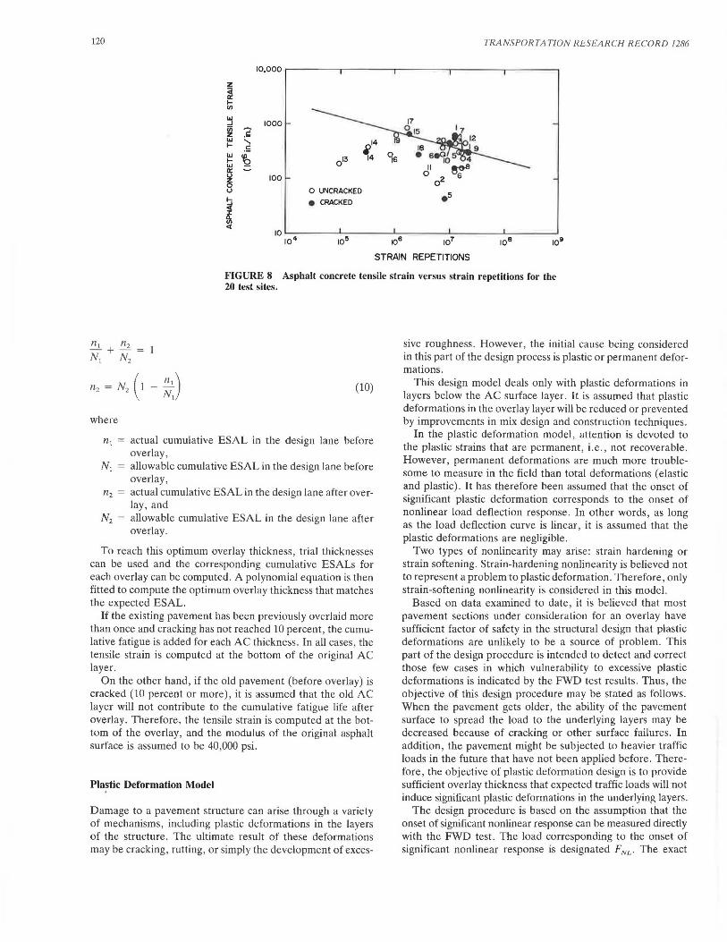
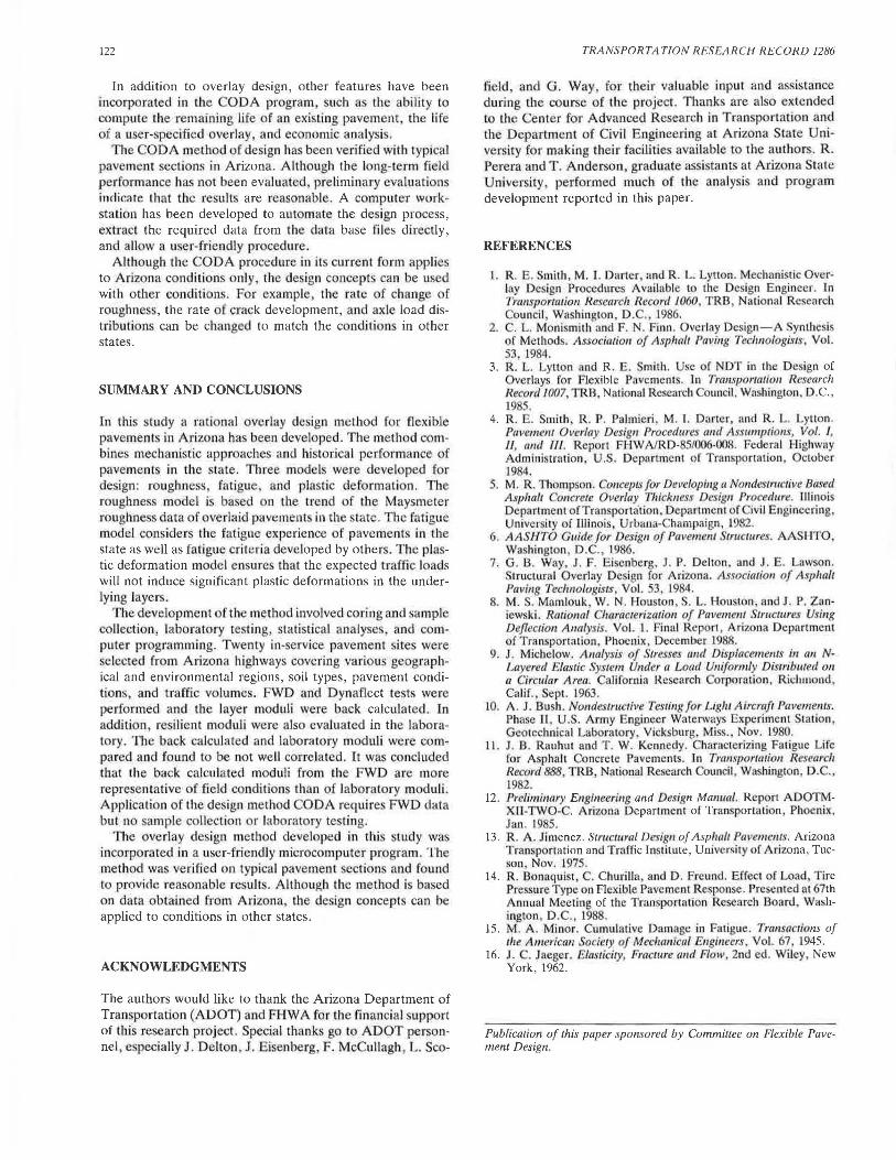
The total adjusted cumulative ESAL was plotted versus the reference tensile strain using a log-log scale as shown in Figure 8. A straight line (fatigue function) was selected close to the upper boundary of the band of previous fatigue functions (11) with a slope of 3.84. This selected fatigue line lies above most of the uncracked pavement sections, which indicates that

uncracked sections have some remaining life. A few uncracked sections lie above the fatigue line, and several cracked sections lie below the line, which indicate some discrepancies. These discrepancies are, however, considered acceptable. The equa­tion of the selected fatigue function is

( )

3 .84

N = 9.33 x 10-7 -1-

EAc (9)

where

N = theoretical number of ESAL repetitions until fatigue failure, and

EAc = tensile strain at the bottom of the AC layer.

Equation 9 is valid for various conditions such as various regions and temperatures because these conditions were nor­malized to standard conditions. Therefore, if the tensile strain at the bottom of the AC layer is known under these standard conditions, the number of ESAL repetitions until fatigue fail­ure can be computed.

Use of the Fatigue Model

To use the fatigue model, a multilayer elastic program such as Chevron can be used to compute the tensile strain at the bottom of the AC layer caused by a 9,000-lb dual-tire load. The layer moduli can be obtained from the FWD back cal­culation as discussed earlier.

In many cases the pavement is overlaid before it is signif­icantly cracked. Therefore, the remaining fatigue life of the existing pavement has to be considered and added to the overlay life. This calculation can be accomplished by using the concept of cumulative damage (Minor's law) (15). Thus, the optimum overlay thickness is the one that satisfies the following equation.

120 TRA NSPORTATION RESEA RCH R ECORD 1286

10,000 r------.-----~------...----~---~

z ~ I-

"' ~ ii ~

1000

... ...., I- ·= ... ~ I-...

~ 100

0 UNCRACKED .5 e CRACKED

u

i ct

10 10 4 10~ 1()6 107 108 109

STRAIN REPETITIONS

FIGURE 8 Asphalt concrete tensile strain versus strain repetitions for the 20 test sites.

(10)

where

n, actual cumulative ESAL in the design lane before overlay,

N 1 allowable cumulative ESAL in the design lane before overlay,

n2 = actual cumulative ESAL in the design lane after over­lay, and

N2 = allowable cumulative ESAL in the design lane after overlay.

To reach this optimum overlay thickness, trial thicknesses can be used and the corresponding cumulative ESALs for each overlay can be computed. A polynomial equation is then fitted to compute the optimum overlay thickness that matches the expected ESAL.

If the existing pavement has been previously overlaid more than once and cracking has not reached 10 percent, the cumu­lative fatigue is added for each AC thickness. In all cases, the tensile strain is computed at the bottom of the original AC layer.

On the other hand , if the old pavement (before overlay) is cracked (10 percent or more), it is assumed that the old AC layer will not contribute to the cumulative fatigue life after overlay. Therefore, the tensile strain is computed at the bot­tom of the overlay, and the modulus of the original asphalt surface is assumed to be 40,000 psi.

Plastic Deformation Model

Damage to a pavement structure can arise through a variety of mechanisms , including plastic deformations in the layers of the structure. The ultimate result of these deformations may be cracking, rutting, or simply the development of exces-

sive roughness. However, the initial cause being considered in this part of the design process is plastic or permanent defor­mations.

This design model deals only with plastic deformations in layers below the AC surface layer. It is assumed that plastic deformations in the overlay layer will be reduced or prevented by improvements in mix design and construction techniques.

In the plastic deformation model, attention is devoted to the plastic strains that are permanent, i.e., not recoverable. However, permanent deformations are much more trouble­some to measure in the field than total deformations (elastic and plastic). It has therefore been assumed that the onset of significant plastic deformation corresponds to the onset of nonlinear load deflection response. In other words, as long as the load deflection curve is linear, it is assumed that the plastic deformations are negligible.

Two types of nonlinearity may arise: strain hardening or strain softening. Strain-hardening nonlinearity is believed not to represent a problem to plastic deformation. Therefore, only strain-softening nonlinearity is considered in this model.

Based on data examined to date, it is believed that most pavement sections under consitleralion for an overlay have sufficient factor of safety in the structural design that plastic deformations are unlikely to be a source of problem. This part of the design procedure is intended to detect and correct those few cases in which vulnerability to excessive plastic deformations is indicated by the FWD test results . Thus, the objective of this design procedure may be stated as follows. When the pavement gets older, the ability of the pavement surface to spread the load to the underlying layers may be decreased because of cracking or other surface failures. In addition , the pavement might be subjected to heavier traffic loads in the future that have not been applied before. There­fore, the objective of plastic deformation design is to provide sufficient overlay thickness that expected traffic loads will not induce significant plastic deformations in the underlying layers.

The design procedure is based on the assumption that the onset of significant nonlinear response can be measured directly with the FWD test. The load corresponding to the onset of significant nonlinear response is designated FNL· The exact

Mamlouk et al.

point at which deviation from linear behavior occurs is difficult to select. Therefore, FNL has been defined as the load at which the load deformation curve deviates 10 percent, measured horizontally, from the straight-line extension of the early por­tion of the curve, as shown in Figure 9.

The detailed step-by-step procedure for the plastic defor­mation overlay design is as follows.

1. Input existing pavement structure geometry, moduli from back calculation analyses, and highway type (Interstate, U. S., or state).

2. Input FWD data for loads from 6 kip to 15 kip or more. Use 6- 12-kip data to establish the straight line (least-squares fit) and check the higher loads for deviation from the straight line at each sensor.

3. If none of the loads shows 10 percent or more deviation, report that FNL is greater than the maximum FWD applied load and bypass plastic deformation design. If one or more loads show deviation 2:::10 percent, proceed to step 4.

4. Use linear interpolation to find the load corresponding to 10 percent deviation (FNL).

5. In comparing the stress states, several different stresses at various points in the underlying layers were considered. The maximum octahedral shear stress, (T0 c1)ma» in the subgrade was chosen because it reflects all the components of the stress tensor (16). Therefore, use Chevron program with FNL applied to the FWD plate to calculate the maximum T 0 e1 that occurs in the subgrade.

6. Determine the design load (Fdes), which is the load on a dual wheel that can be used in checking the adequacy of a trial overlay design thickness. The value of Fdes is chosen so that the probability of an actual dual wheel load exceeding this value is very small. The degree of conservatism in thi part of the design can be controlled through the choice of this probability. A sample of axle loads obtained from Arizona highways showed that the selected probabilities were 0.00001, 0.00008, and 0.00008 for Inter tate, U.S., and state highways, respective ly. These probabilities resulted in an expected num­ber of dual wheel load values exceeding Fdes of about seven in 1 year.

7. Use Chevron program with Fdes applied to a dual wheel and calculate the maximuin T0 c1 in the subgrade.

A

LOAD

DEFORMATION

FIGURE 9 Nonlinearity of underlying layers and definition of onset of significant nonlinear response.

121

8. H -r,"1 caused by F,1<-< is less than or equal to -r0 c1 caused by FNL report this fact and bypass plastic deformation de ign. If not, proceed to step 9.

9. With the overlay obtained from fatigue analysis in place , use Chevron program with F,,., applied to a dual wheel and calculate -r0 cr in the subgrade.

10. If T0 c1 in step 9 is less than or equal to T because of F Nu

the pavement is safe against plastic deformation with the over­lay. If T0 c1 in step 9 is more than 'T 0 c1 caused by FNL> proceed to step 11.

11. Increment the thickness of the overlay in steps until -r0 c1

caused by Fd,,, is equal to T0 c1 caused by FNL·

The preceding step-by-step procedure including compu­tation of TQ<I ha been programmed in the CODA program . The needed parameters have been fixed and the entire plastic def rmation design procedure ha. been automated. The u er i. required only to input the data indicated in tep l and 2. Of cour e, modifications to the • fixed value ' can be made readily to the program if desired. Users who desire to u e the plastic deformation model independent of the fatigue analy is should proceed to step 11 after tep 8.

It should be noted that the plastic deformation model deserves to be cal.led mechanistic becau e it add.re es permanent defonnation a particular mechanism of damage. Even though ome plastic deformation occurs with every l ad application,

the intent of this procedure i to keep the plastic deformation small . Thi intention corresponds to an attempt to maintain the deformations almo t entirely within the ela tic range. An extension of this method to include an e timate of th "expected life ' of a pavement structure with respect to plastic defor­mation, i theoretically possible. However, the art and science of predicting pla tic deformations is not sufficiently well devel­oped to ju ·tify thi extension at the present time.

Complete Overlay Design

The three models-roughness, fatigue and pla tic defor­mation-were incorporated in the overlay microcomputer program ODA. The traffic load requirement in this method of overlay de! ign i · the cumulative 18-kip ESAL in the design lane during the de i~n period. ome exi ting pavement con­dition parameter are also needed, uch a May meter rougb­ne reading and cracking. Pavement layer thickne ·se , mate­rial type previ.ous overlays, if any and year of con truction are also needed.

ince both fatigue and plastic deformation models require the knowledge of pavement and ubgrade layer moduli the first step in the procedure is lo run the FWD test on the pavement section under con ideration. The fatigue mod I requjres performing the FWD te t at a load level of 9 0 0 lb only, wherea thepla tic deformation model (if used) requires ruJming the FWD tc tat several load levels as discus ed earlier.

The FWD deflection data at a 9,000-lb load level are further used to back calculate the pavement and ubgrade .layer mod­uli. Since the modulu. of the AC layer is significantly affected by temperature a subroutine wa develope I in th CODA program to adjust the A modulus to a standard temperature of 70°F based on the AA HTO guide (6).

122

In addition to overlay design, other features have been incorporated in the ODA program , uch a. the ability to compute the remaining life of an exi ting pavement , the life of a u er-specified overlay, and economic analysis.

The CODA method of design bas been verified wilh cypicaJ pavement ·ections in Arizona. Although the I ng-rerm field performance bas not been evaluated , preliminary evaluations in<lir.::ire that the results are reasonable. A computer work­station has been developed to automate the design process, extract the required data from the data base files directly, and au w a u ·er-friendly procedure.

Although the ODA procedure in it current form appli to Arizona conditio.n only the design concepts can be u ed with other conditi.on . For example, the rale of change of roughness, the rate of crack development, and axle load dis­tributions can be changed to match the conditions in other states.

SUMMARY AND CONCLUSIONS

In this study a rational overlay de ign method for flexible pavements in Arizona ha. been developed . The method com­bine mechanistic approaches and historical performance of pavemenr in the state. Three mode l were developed for de ign: roughness fatigue, and pla tic deformation . The roughness model i based on the trend of the Maysmeter roughnes · data of overlaid pavi;ment in the. late. The fatigue model considers the fatigue experience of pavement in the state as well as fatigue criteria developed by others. The plas­tic deformation model ensure that the expected traffic loads will not induce significant plastic deformations in the under­lying .layers.

The developmen t of the metbod involved coring and sample collection, laboratory testing, statistical analyse · and com­puter programming. Twenty in-service pavement sire were selected from Arizona highways covering various geograph­ical and environmental regions, soil types, pavement condi­tions, and traffic volumes. FWD and Dynaflect lestli were perfonned and the layer moduli were back calculated. In addition, re ilient moduJi were also evaluated in the labora­t0ry. The back calculated and laboratory moduli were com­pared and found to be not well corre:lated. lt wa concluded that the back calculated moduli from the FWD are more representative of field condition than of laboratory m duli. Application of the design method ODA requires FWD data but no ample collection or laboratory te ting.

The overlay de ign method deve loped in this tucly was incorporated in a user-friendly microcomputer program . Th method was verified on typical pavement ection and found to provicfe reasonable result . Allbough the method is based on data obtained from Arizona the design concepts can be applied to conditions in other states.

ACKNOWLEDGMENTS

The authors would like to thank the Arizona Department of Tran portation (ADOT) and FHWA for the financial supp rt of this research project. Special thanks go to ADOT per-on­nel , especially J. Delton , J. Eisenberg F. McCuJiagh L. co-

TRANSPORTATION RESEARCH RECORD 1286

field, and G. Way for their valuable input and assistance during the course of the project. Thanks are also extended l tl1e Center for Advanced Research in Tran portati n and the Department of Civil Engineering at Arizona tale Uni­versity for making their facilities available to the authors. R. Perera and T. Anderson, graduate a istant at Arizuna tate University , performed much of the analysis and program development reported in this paper.

REFERENCES

1. R. . Smith , M. I. Darter, and R. L. Lytton . Mechanistic Ove r­lay Design Procedures Available to the Design Engineer. In Trmrsportation Rese(lrch Re ord 1060, TRB , National Research Council, Washington , D.C., J986.

2. C. L. Moni mith and F. N. Finn. Ove rlay Design-A Synthe i of Methods. Association of Asphalt Paving T11clr11ologis1s , Vol. 53 1984.

3. R. L. Lylton and R . E. Smith. U e of DT in the D esign of Overlays for Flexible Pavements. Jn Tran.wortatio11 Research Record 1007, TRB. National Research ouncil , Wa hingron . D .C., 19 - .

4. R. E. Smith, R . P . Palmieri , M. T. Darter, and R . L. Lytton. P11ve111e111 Overl"Y Design Procedures and Assumptions, Vol. I, II, and /II. R port FHWA/RD-85/006·008. Federal Highway Administration. U .. Department o( Tran p rtalion, October 19 4.

S. M. R. 111ompson. Concepts for Developing a Nondestru,·tive Based Asphalt Concrete Overl"Y 111icknes Design Procedure. Illinois Department ofTrnnsporta'tion Department of Civil Engineering, University of Illinois, Uruan - hampaign, L982.

6. AASHTO Guide for Design of Pavement Str11c111re . AASHTO, Washington D .. , L986.

7. G. B. Way J . F. Ei enberg, J . P. Delton and J.E. Lawson. Structurnl Overlay De ign for Arizona. Associmion of Asplr"lt Paving Teclmologists , Vol. 53, 1984.

8. M. S. Mamlouk W. N. Houston , S. L. H.011 ton , and J . P. Zan­iewski. Rational haracterization of Pavement Structures U. i11g Deflection Analysis. Vol. I. Final Report , Arizona Department of Tran portation , Phoenix , December 1988.

9. J. Michelow. Analysis of Slre ·ses and Displacements in an N­La ered Elastic System Under a Load Uni/ ormly Distributed 011

a Circular Are<1. California Research rporation, Ricl1111ond, Calif., ept. 1963.

10. A. J. Bu h. Nonde lmcrive Testing for Light Aircraft Pm1oments. Phase H, U .. Army Engineer Waterways Experiment Station, Geotechnical Laboratory Vick burg, Miss. ov. 1980.

U. J . B. Rauhut and T. W. Kennedy. haractcrizing Fatigue Life for Asphalt oncrete Pavements . . In Transportation Resetirc/1 Record 888, TRB, National Research Cow1cil , Washington, D.C., 1982.

12. Pre/imi11t1ry Engineering and Design Ma1111(1l. Report ADOTM­Xfl-TWO· . Arizona Department of Transportation, Phoenix, Jan. 1985.

13. R . A. Jimenez. Strucwral Design of Asphalt Pavements. Arizona Tran portation and Traffic Institute , Univcr.~i1y of Arizona, Tuc­son, Nov. 1975.

14. R. Bonaqui t, . Churilla and D. Freund. Effect or Load, Tire Pre urc Typ ·on Flexible Pavcmeni Response. Presented at 67th Annual Meeting of the Tran portation Research Board. Wa~h­ington , D . ., 19 .

15. M. A. Minor. Cumulative Damage in Fatigue. Trcmsacrions of tlie Americ;(ln Sot.icty of Mechanical E11gi11eers , Vol. 67, 1945.

16. J. C. Jaeger. Elasticity Fracture and Flow, 2nd ed . Wiley, New York , 1962.

Publication of this paper sponsored by Cammi/lee on Flexible Pave­ment Design.