outsourcing, firm innovation, and industry dynamics in the ... · outsourcing, firm innovation, and...
TRANSCRIPT

Outsourcing, Firm Innovation, and
Industry Dynamics in the Production of Semiconductors
Jeff Thurk*
March 2019
PRELIMINARY
Abstract
I build a dynamic oligopoly model to identify the factors which explain the increase in factoryless
production in the global semiconductor industry. Firms enter the industry each period and
choose whether to invest in developing proprietary fabrication facilities or instead outsource
production to a competitive third-party fabrication industry. The estimated model demonstrates
that factoryless production enables firms to significantly reduce upfront capital expenditure
thereby lowering the costs of entry. The increasing availability of venture capital investment
also played an important role, while the possibility of growth through future R&D investment
and the benefits of lower production costs, due to sourcing either domestically or globally, had
little impact on equilibrium entry. Factoryless and integrated firms co-exist in the long run
equilibrium since the latter firms are able to vertically differentiate their products, enabling
them to maintain significant market share despite significant entry of factoryless firms.
* I thank Victor Aguirregabiria, Tom Holmes, Mathew Mitchell, Amil Petrin, Benjamin Pugsley, Mar Reguant,Joel Waldfogel, and Kevin Williams for comments and suggestions as well as conference participants at the 2018Barcelona GSE Summer Forum and the Society for Economic Dynamics at Mexico City. I also thank ShrikantLohokare and Jessica Mueller at the Global Semiconductor Alliance. Financial support was provided by theInstitute for Scholarship in the Liberal Arts at the University of Notre Dame. All errors are my own. Corre-spondence: University of Notre Dame, Department of Economics, Notre Dame, IN 46556. E–mail: [email protected];http://www.nd.edu/ jthurk/.

1 Introduction
Over the past forty years the world has become much more integrated as reductions in trade costs
due to technological advancements (Hummels, 2007) and import tariffs (Bergstrand, Larch, and
Yotov, 2015) increased bilateral trade significantly. An important feature of this increase in trade is
that roughly two-thirds of international trade occurs in intermediate inputs (Johnson and Noguera,
2017) which indicates that global supply chains have become an integral part of the world economy.
Much of this is driven by vertical specialization as different countries vie for segments of the global
supply chain which align with their comparative advantage (Hummels, Ishii, and Yi, 2001). All of
this serves to point out the quantitative importance of global supply chains and the importance of
understanding the impact of sourcing decisions upon not only firm production costs but also the
subsequent decisions that lower marginal costs may enable (Antras, Fort, and Tintelnot, 2017). The
impact of sourcing on the evolution of industries, particularly the role of sourcing in influencing the
equilibrium entry and exit decisions of firms and the subsequent evolution of the industries they
inhabit, is not well understood, however.
I study the impact of sourcing on firm entry and exit in the semiconductor industry –
an industry which produces goods (e.g., microprocessors) which enable nearly every facet of our
modern digital life. The industry is highly-competitive and fast-paced as firms dedicate substantial
resources towards creating new products. It has also changed substantially over the years as
technological innovations increased the performance of its products and growing demand led to
increases in industry revenue as well as the number of firms.1 During the 1970s and 1980s, the
industry was dominated by vertically-integrated device manufacturers (IDMs) which managed all
components of the value chain (design, fabrication, testing, and distribution) in-house. Vertical
integration provides these firms an opportunity to coordinate all facets of production and helps
ensure the protection of intellectual property. These firms operate fabrication facilities around the
world to take advantage of the comparative advantages (including tax benefits) offered by different
countries.
While IDMs produce in-house (and potentially off-shore production elsewhere), an increas-
ingly popular business model is to outsource all production to third-party, low-cost foundries
overseas, largely Taiwan and China. Firms choosing this business model lack an internal fabrication
facility and are known as “Fabless.” Today, Fabless firms account for roughly 90% all semicon-
ductor firms and generate one-third of industry revenue. The Fabless business model proposes
two advantages to the traditional IDM. First, outsourcing fabrication enables these firms to avoid
the substantial capital investment required to build a fabrication facility. Second, outsourcing,
often overseas, enables these firms to take advantage of scale to lower input costs as they pool
production with other Fabless firms in third-party foundries. Outsourcing overseas also enables
1 This amounts to a financial corollary to Intel founder Gordon Moore’s 1965 prediction, known as “Moore’s Law”,that the processing power of an integrated circuit doubles every year.In 1975 Moore amended his prediction to everytwo years – a prediction that fit the data amazingly well until 2012 when the pace of technological improvementsbegan to slow.
– 1 –

firms to reduce take advantage of lower foreign wages and weaker environmental standards. Thus,
the Fabless business model is thought to decrease upfront costs as well as on-going production costs.
Unfortunately, it also constrains the degree of specialization embedded in a product and exposes
the firm to imitation risk. Consequently, it is unclear whether there exists a clear dominant business
strategy, IDM or Fabless, in the long-run; or perhaps the two can coexist as they offer similar but
differentiated products for consumers.
My objective is to evaluate the impact of outsourcing on the firm dynamics in this high-
tech industry. To do so I develop a dynamic oligopoly model in which firms strategically choose
whether operate in-house fabrication facilities or outsource production to a perfectly-competitive
third-party fabrication industry. To account for changing exogenous upfront entry costs, on-going
production costs, and industry growth; I consider firm strategies which vary over time as the
industry transitions between long-run equilibria. Therefore, the equilibrium concept I adopt is
a non-stationary modification to the Moments-based Markov Equilibrium (MME) of Ifrach and
Weintraub (2016). In a MME, firms have limited capacity to monitor the entire distribution of
rivals and instead focus on a few sufficient statistics. In a non-stationary MME (nMME) I maintain
this assumption but allow for the industry to transition between two long-run MME equilibria. The
first MME provides a starting point for the initial industry state while the second stationary MME
provides firms information for their long-run value function. Importantly, the second stationary
MME need not be contained in the data but can rather occur at an arbitrary future date provided
one is willing to assume that model primitives which had induced the transition are fixed, or
equivalently are growing at a constant rate.
In the first stationary MME the implicit assumption is that not only is the industry in
a stationary MME but also that the changes in the industry which drive the transition to the
second stationary MME are unexpected. In my setting this is the establishment of the first
“pure play” foundry, Taiwan Semiconductor Manufacturing Company (TSMC), by Morris Chang
in 1987. Chang, a Ph.D. electrical engineer trained at Stanford, had risen through the ranks at
Texas Instruments, one of the largest IDMs, until ultimately becoming head of all semiconductor
operations at the company. At a time when most people might have considered retirement, he was
recruited by the Taiwanese government to found TSMC with the intent of boosting the country’s
high-tech sector in order to compete with firms in Japan and the United States.
Unitl TSMC’s founding, innovation appeared to be limited as entrepreneurs equipped with
good ideas lacked the immense capital required to make their designs a reality:
When I was at TI and General Instrument I saw a lot of IC designers wanting to leave
and set up their own business, but the only thing, or the biggest thing that stopped
them from leaving those companies was that they couldn’t raise enough money to form
their own company. Because at that time it was thought that every company needed
manufacturing, needed wafer manufacturing, and that was the most capital intensive
part of a semiconductor company, of an IC company. And I saw all those people wanting
– 2 –

to leave, but being stopped by the lack of ability to raise a lot of money to build a wafer
fab.
Furthermore, the location of TSMC in Taiwan played to the country’s comparative advantage:
We had no strength in research and development, or very little anyway. We had no
strength in circuit design, IC product design. We had little strength in sales and
marketing, and we had almost no strength in intellectual property. The only possible
strength that Taiwan had, and even that was a potential one, not an obvious one, was
semiconductor manufacturing, wafer manufacturing. And so what kind of company
would you create to fit that strength and avoid all the other weaknesses? The answer
was pure-play foundry.
This speaks to the changing role of the boundary of the firm enabled by international trade (Atalay,
Hortacsu, Li, and Syverson, 2017). In the model, I treat the Taiwanese government’s to develop
TSMC as an exogenous and unforeseen (to the rest of the IDM semiconductor firms) shock in the
industry.
The model serves two purposes. First, I use it as a theoretical framework to identify four
potential channels which drive outsourcing. First, the model predicts that outsourcing can enable
entry of small firms by reducing the upfront costs of commercializing their product. Put differently,
the model predicts that outsourcing may relax liquidity constraints facing firms much in the same
way a government subsidy on capital expenditure lowers the cost of market entry. Second, I show
that when outsourcing reduces marginal costs of production, firm profits may increase leading to
greater discounted future profits. The degree to which profits increase due to outsourcing, however,
depends on the endogenous market power of the firms, or equivalently the degree to which reductions
in cost are passed-through to consumers (Weyl and Fabinger, 2013). Third, outsourcing overseas
to take advantage of lower variable costs (e.g., wages) further increases the expected value of entry.
Finally, if Fabless firms are able to lever their reduced capital expenditure and lower marginal costs
to invest in research and design, future growth opportunities may be brighter for an outsourcing
firm relative to a vertically-integrated IDM.
Put together, I use the model to demonstrate that outsourcing may encourage market entry
by both lowering costs and increasing pay-offs and that these effects are particularly relevant for
small firms who normally would not have been able to secure financing through other market
mechanisms such as venture capital.2 For an incumbent firm, the model predicts that, all else
equal, an increase in discounted profits due to outsourcing increases the willingness to stay in the
market.
As the model is also tractable, the second purpose is to test the quantitative significance of
these predictions. I do so by estimating the model using proprietary data from the semiconductor
2 Venture capital firms are often the primary investors in the high-tech industry but they also require a returnon investment of roughly 10x and have short investment horizons (5-7 years) so securing financing to cover theproduction of a new but not revolutionary chip design is practically infeasible.
– 3 –

industry, including detailed wafer pricing data which enable me to identify the cost savings firms
enjoy by outsourcing production abroad. The estimated model replicates moments in the data well
and generates reasonable and statistically significant parameter values. I show that the growth of
outsourcing was largely due to the ability of firms to avoid the large cost of building a fabrication
facility rather than lower production costs due to economies of scale from third-party facilities,
either domestic or abroad, or future growth possibilities from conducting research. I also find
that the industry’s evolution is sensitive to changes in the venture capital industry which would
have impacted financing rates and therefore capital expenditure costs. These results indicate that
outsourcing amounted to a new financial technology which decreased entry costs and enabled entry
of smaller companies. Increased entry of Fabless firms ultimately led to increased competition for
the traditional, vertically-integrated IDMs leading to less profits for these firms.
Finally, I use the estimated model to forecast the long-run evolution of the industry. I show
that vertical-differentiation between IDM and Fabless firms enables the two business models to
co-exist. The long-run industry equilibrium is therefore best characterized as one in which IDMs
account for only 20% of semiconductor firms though they generate 60% of industry revenue.
Related Literature. In this paper I empirically investigate the impact of outsourcing production
overseas on the dynamics of an industry in which innovation is driven by both incumbent firms
and new entrants. As such I contribute to two branches of economics: industrial organization and
international trade.
The closest paper is that of Igami (2018) who uses a dynamic oligopoly model to explore
the incentives of firms to offshore in the hard disk drive industry. This paper is, however, different
in three dimensions. First, my focus is on outsourcing rather than offshoring so my contribution
is to show how globalization redefines the boundaries of the firm as well as its span of control
(Lucas, 1978). Second, firms produce differentiated goods in this industry (and in the model) which
provides for the long-run co-existence of both IDM and Fabless firms. Third, my objective is to
use the estimated model to evaluate the relative contributions of each channel towards explaining
the relative roles each played. This also enables me to identify an important mechanism which
further increased market entry of these firms: venture capital. This is an important finding since
there exists few empirical studies in the literature which quantify the merits of the venture capital
industry despite the fact of its omnipresence in innovation epicenters such as Silicon Valley, CA
and Seattle, WA.
As an empirical model of dynamic oligopoly, the paper aligns with the models of firm
innovation such as Goettler and Gordon (2011), Ryan (2012), Collard–Wexler (2013), and Igami
(2017, 2018). As in Goettler and Gordon (2011) and Igami (2017, 2018) my estimates are based on
solving the static and dynamic parameters simultaneously – what has become known as the “full-
solution approach.” While this increases the computational burden, it also alleviates endogeneity
– 4 –

concerns which may arise when employing a two-step estimation as in Bajari, Benkard, and Levin
(2007).3
In the semiconductor industry, early studies focused on the patenting motives4 while later
studies have focused on linking patenting behavior with R&D expense. Hall and Ziedonis (2001) is
the most relevant paper to this one. The authors reason that the aggregate data used in Kortum and
Lerner (1998) hid industry-specific effects of the shift in patent protection. Using both empirical and
survey evidence, they conclude that patent reform had two effects. First, it promoted fragmentation
by enabling fabless firms to enter and secure their place in the industry. Second, it resulted in large
firms becoming engaged in patent portfolio races in order to streamline future innovation.5
This paper also contributes to a growing literature on the importance of international
markets and global supply chains. Here, the closest paper is Antras, Fort, and Tintelnot (2017)
who study the interaction of global sourcing on firm production costs and export decisions. My
contribution is to study extend the analysis of global supply chains to entry decisions and industry
dynamics.
The remaining paper is structured as follows. In Section 2, I present information about the
global Semiconductor industry and discuss important defining features of the data. In Section 3, I
present the dynamic oligopoly model and discuss how I extend the MME to a non-stationary setting.
Section 4 provides details on the estimation and presents the estimation results. In Section 5, I
use the estimated model to measure whether the increase in factoryless production was due to
reductions in upfront costs; lower on-going production costs due to sourcing from either domestic
or global third-party facilities; or future growth prospects from investments in research & design.
I also discuss the long-run equilibrium implications of factoryless production in this industry. I
provide concluding remarks and discuss areas for further research in Section 6.
3 See Berry and Compiani (2017).4 See Tilton (1971), Taylor and Silbertson (1973), Levin (1982), and von Hippel (1988).5 Their results are supported by Hunt (1996), who finds evidence of a significant shift in competition during the late
1980s or early 1990s. Whereas reverse-engineering had previously enabled innovations to diffuse to competitors,his empirical results indicate that semiconductor firms moved to protect their innovations with patents. Theconsequence was a shift towards creating next-generation technologies based on competitors’ licensed, rather thanimitated, ideas.
– 5 –

2 The Semiconductor Industry
In this section I discuss details of the semiconductor industry and pay particular attention areas
which map to model. Semiconductor firms are those firms engaged in the design and/or fabrica-
tion of semiconductors – any material whose electrical conductivity has values between that of a
conductor and a insulator. Integrated circuits (ICs) comprise the bulk of industry revenue6 and
are generally considered any network of transistors fabricated on a surface to process binary data
by switching on and off.
The semiconductor industry forms the backbone of the hi-tech industry, hence is a prime
driver of economic growth. For example, the industry’s $204 billion in 2004 global sales, enabled
$1.2 trillion in electronic systems business and $5 trillion in business services, or approximately
10% of global GDP.7 While the industry provides products for a wide-variety of hi-tech sectors,
personal computers still account for the majority of industry sales.
There are four kinds of products in the industry; three of which I include in the analysis
(Table I). Firms such as Intel and Advanced Micro Devices (AMD) produce microprocessors which
amount to integrated circuits containing one or more central processing units (CPUs). Example
products include personal computers, tablets, and servers. The 32- and 64-bit microprocessors
in PCs and servers are based on x86, POWER, and SPARC chip architectures while tablets are
usually based on an ARM chip architecture. Less powerful microprocessors (e.g., 8, 16, and 24-bit)
are often employed in toys and vehicles.
Table I: Semiconductor Firms and Products
Semiconductor Products Example Firms Example End-Products
1. Microprocessors AMD, Intel, ... Computers, servers
2. “System on a Chip” Broadcom, Nvidia, Qualcomm, ... Mobile phones
3. Commodity integrated circuits Analog Devices, Xilinx, ... Bar code scanners
4. Memory IBM, Samsung, Toshiba, ... Computers, flash drives
The second category “system on a chip” (or SoC) is the newest kind of semiconductor chip as
it combines all the necessary components for an entire system on a single chip. These products are
popular among small devices such as smartphones as they integrate CPUs with graphics, camera,
as well as audio and video processing. Primary firms in this market include Nvidia, Broadcom,
Qualcomm.8 The third category included in the analysis is commodity integrated circuits commonly
used in simple technological devices such as bar code scanners. The final category commonly
6 ICs accounted for 85% of total industry revenue in 2004 - World Semiconductor Trade Statistics, “WSTS Semicon-ductor Market Forecast, Autumn 2004,” Press Release, November 2, 2004. (www.wsts.org).
7 http://en.wikipedia.org/wiki/Semiconductor industry8 To further indicate the importance of this industry: In early 2018 Singapore-based Broadcom attempted a hostile
takeover of Qualcomm ($120 billion) which was later invalidated for national security reasons by the Trumpadministration. Intel has since expressed interest in acquiring Qualcomm to solidify its position to deliver 5gmobile services in the future.
– 6 –

commonly considered as part of the industry is the area of memory chips, particularly flash memory
which are produced by large technological conglomerates such as IBM and Samsung. As these
companies create a large array of products outside the industry, identifying the importance of
outsourcing towards the evolution of this product group was difficult and I therefore excluded them
from the analysis.
There are four primary components of the value chain: design, fabrication, testing, and
sales/ distribution. During the design stage, skilled design engineers construct prototypes of next-
generation chips using high-end, expensive electronic design automation (EDA) software. Upon
completion, these plans are delivered to a potentially external fabrication facility where the chip
circuits are constructed in successive layers on the surface of a flat silicon wafers. Firms which
conduct this stage internally must incur a large fixed capital investment (≈$2 billion) to build a
plant (a “fab”) consisting of a wide variety of expensive equipment capable of building the chips
under extreme environmental requirements for cleanliness. During the Assembly stage, the wafers
are split into individual chips (a “die”) for distribution to customers.
Comparative advantage comes through innovation and innovation is a fast-paced, cumula-
tive effort in which tomorrow’s new product depends heavily on a broad set of today’s products
and ideas. In a 1965 paper, Intel co-founder Gordon E. Moore noted that the capabilities of the
integrated circuit doubled roughly every 18 months.9 This prediction became known as “Moore’s
Law” and has held remarkably true in the 40 plus years since. Moore’s Law also speaks to the
short-life associated with any current product and the need to develop tomorrow’s great idea
today. Accordingly, R&D comprises a significant component of firm expense and this dependence
has increases from 11% of firm sales in the early 1980s to 31% of firm sales for the period 2000-2005.
2.1 A Changing Marketplace
Semiconductor firms tend to be large and international in scope, with most of the major players
located in Japan, Korea, and the United States. In Figure 6 I document that the industry has
undergone a significant transformation. In panel (a) I document that total industry sales have grown
substantially since the early 1990s, driven primarily though increasing expenditures on personal
and commercial information technology. Concurrent with this growth was a shift in business model
from vertically integrated device manufacturers (IDMs) towards niche design firms which outsource
manufacturing to low cost fabrication plants. Since this latter group lacks any kind of production/
fabrication abilities, they became known as as “fabless.” Today, roughly one-third of all industry
revenue is generated by fabless firms. In panel (b) I document the dramatic increase in Fabless
entry after the establishment of TSMC, particularly in the later 1990s. Whereas nearly every firm
prior to TSMC’s establishment was vertically-integrated, 90% of all firms today are Fabless – a
dramatic shift.
9 At the time, he was referring to the number of transistors a firm could inexpensively place on a single silicon wafer.Today, advancement generally refers more generically to processor speed.
– 7 –

Figure 1: A Growing and Changing Industry
0
50
100
150
200
250
300
350
400
450
Rev
enue
($2
010
Bn)
1980 1985 1990 1995 2000 2005 2010 2015
Year
Compustat WSTS
Total Industry Revenue
(a) Total Industry Revenue
TSMC Established (1987)
020406080
100120140160180200
Num
ber
of E
ntra
nts
1980 1985 1990 1995 2000 2005 2010 2015
Year
IDM Firms Fabless Firms
Market Entry by Type
(b) Firm Entry
Notes: In panel a, I present total industry revenue over time using two different approaches. In the solid line Ipresent the time series based on Compustat financial information for firms identifies as semiconductor firms bythe Global Semiconductor Alliance. In the dashed line I present the time series based on industry equity analysts(source: WSTS Semiconductor Market Forecast Autumn 2017). In panel b, I present the time series of firm entryfor IDM and Fabless firms (source: Global Semiconductor Alliance).
2.2 An International Market for Semiconductor Fabrication
Growth of the fabless business model (i.e., of outsourcing) is predicated on the ability of firms to
produce quality goods at efficient scale. Outsourcing fabrication is particularly attractive in this
industry as semiconductors tend to be high value but weigh little thereby incurring little trans-
portation cost. As many low-wage countries lack the technical expertise and capital infrastructure
to establish viable foundries, most foundries are located in a small set of countries including China,
Europe, Japan, Taiwan, and the United States (Table VI). While the vast majority of outsourcing is
done overseas (where Taiwan accounts for approximately 59% of all outsourced wafers produced),
the United States foundries account for four percent of all third-party wafers produced. This
indicates that global supply chains have played an important though not necessarily pivotal role in
facilitating growth of the fabless business model.
The majority of third-party foundries which produce Fabless products are located in South-
east Asia (Table II). The common story for this concentration is that these countries have a
sufficiently skilled workforce to enable the complex production of semiconductor wafers while low
wages and relatively weak regulations (e.g., environmental standards) enable low-cost production
without sacrificing much in terms of quality. I quantify the reductions in production cost from
outsourcing using data on semiconductor wafer fabrication prices attained from a proprietary
database collected by the Global Semiconductor Alliance (GSA). The GSA is a nonprofit industry
organization consisting of fabless firms. Each quarter the organization surveys its members to collect
information on prices, quantities, and characteristics of their orders from both domestic and foreign
foundries. Responses are anonymous and firms which participate are granted access to the results.
The dataset consists of 14,692 individual quarterly responses to the “Wafer Fabrication & Back-End
– 8 –

Table II: Fabless Production Market Share by Country
Year China Japan Korea Singapore Taiwan USA Other
2004 11.07 6.07 5.78 14.56 45.42 3.75 13.352005 2.47 4.89 2.47 6.04 69.06 2.66 12.412006 2.36 7.37 5.58 13.35 57.26 3.54 10.542007 6.38 2.95 3.18 18.74 57.81 2.19 8.752008 6.44 6.42 4.69 14.97 57.90 2.00 7.582009 6.87 6.82 2.22 9.49 64.83 4.30 5.472010 7.42 11.73 3.42 6.90 58.75 7.16 4.622011 13.84 8.02 4.44 4.05 59.07 6.48 4.102012 4.99 4.01 7.43 3.19 68.53 4.45 7.402013 5.97 14.45 5.70 2.83 62.91 3.74 4.402014 9.30 24.09 5.97 5.26 46.31 4.14 4.93
Total 7.17 8.38 4.71 8.70 59.38 4.13 7.53
Notes: Author’s calculation based on GSA wafer pricing survey (2004-2015). Statistics reflect the share ofwafers produced by third-party fabrication facilities in a given year. “Other” includes Europe and othercountries with small market shares (e.g., India, Israel).
Pricing Survey” covering years 2004-2015. According to GSA the sample is representative of the
industry and accounts for roughly one-fifth of all fabless semiconductor wafers produced worldwide.
The data include nominal price paid, the number of wafers purchased, and the foundry’s
country location. I also observe characteristics about the wafer, including the line width, wafer
size, and number of layers. I can therefore examine how foundry wafer prices vary by foundry
location after controlling for physical characteristics. U.S. foundaries produced on average 3.96%
of the wafers during the sample. In comparison, fabrication plants in Taiwan, Singapore, and China
accounted for 58.22%, 9.06%, and 7.42% of the market, respectively. I cannot identify the specific
foundry which fulfilled each order though the dominance of Taiwan Semiconductor Manufacturing
Corportation (TSMC) in the Taiwanese market, Semiconductor Manufacturing International Cor-
poration (SMIC) in Chinese market, and Chartered Semiconductor in Singapore market suggests
that transactions which involve wafers fabricated in the Taiwan, Chinese, and Singapore markets
where fulfilled by these firms. Thus, while there are a variety of foundries producing semiconductor
wafers for fabless semiconductor firms, the bulk of the wafers are produced overseas in Taiwan,
presumably by TSMC.10
The data therefore enable me to evaluate differences in production cost (proxied by foundry
price) across countries. I can therefore estimate the price of fulfilling an order with a US-based
foundry versus a foundry based in Asia. If one is willing to assume that the US foundry price
is a good approximation for the marginal cost of producing in-house, the estimated differences in
foundry prices also pins down the cost benefits underlying outsourcing.
In Table III I present a series of hedonic price regressions to uncover why TSMC has such
dominant market share. In column (1) I project log price onto foundry location using foundries
located in the United States as the reference category and only controlling for differences in price
over time via year fixed effects. This regression explains little about the variation in price (low R2)
10Unfortunately, there is no information regarding buyers.
– 9 –

Table III: Cost Advantages of Outsourcing
dep: log(Price) (1) (2) (3) (4)
China/ Taiwan -0.2695***(0.0328)
China -0.2845*** -0.5108*** -0.5152***(0.0397) (0.0304) (0.0310)
Taiwan 0.2752*** -0.2366*** -0.2469***(0.0285) (0.0339) (0.0342)
Malaysia -0.4033*** -0.5883***(0.0775) (0.0629)
Singapore -0.1096** -0.3320***(0.0347) (0.0358)
Metal Layers 0.1142*** 0.1200*** 0.1279***(0.0060) (0.0060) (0.0061)
Process Masks 0.0114*** 0.0117*** 0.0120***(0.0011) (0.0011) (0.0011)
Poly Layers 0.0306** 0.0206 0.0069(0.0108) (0.0115) (0.0119)
lnQ -0.0464*** -0.0471*** -0.0513***(0.0027) (0.0029) (0.0029)
Constant 6.9291*** 6.7414*** 6.7403*** 6.7345***(0.0274) (0.0518) (0.0510) (0.0519)
Time FEs X X X XProduct FEs X X X
R2 0.0743 0.8022 0.8003 0.7930N 10,685 10,685 9,468 9,468
Notes: Table presents projections of log wafer price onto foundry location controlling for locations. Referencecategory is foundries located in the United States. Robust standard errors reported in between parentheses withp-values denoted by * p < 0.10, ** p < 0.05, and *** p < 0.01.
and suggests TSMC actually charges a higher price relative to U.S. foundries. In the remaining
columns I include covariates for product characteristics as well as product-level fixed effects which
I define as the process size and wafer size pair.
Including product characteristics increases the models’ overall fit dramatically. We also
observe intuitive coefficients on product characteristics where increasing the number of metal layers,
process masks, or poly layers increases the complexity of the production process leading to a higher
price. The industry also appears to offer quantity-discounts as larger orders lead to lower prices.
Adding product characteristic information has no qualitative effects on the estimated dif-
ferences in price across foundries located in different countries. We still observe substantial price
variation by location where wafers produced in China overseas are half as expensive to produce as
in the United States while contracting with TSMC amounts to a 24% reduction in price. When
I restrict attention to just variation between fabless contracts in the United States, China, and
Taiwan (i.e., the majority of the observations) we observe that contracting with a foundry in the
– 10 –

either China or Taiwan is 26.95% less expensive than contracting with a foundry in the United
States – a significant cost advantage.
The fact that foreign countries can produce products less expensively is a necessary but
not sufficient condition for outsourcing and there are additional factors which facilitated growth
of the Fabless business model. First, doing business overseas can be expensive since doing so
requires shipping finished product back to the United States and paying any relevant import duties.
An additional motivating factor therefore is the fact that international trade costs have fallen
significantly since the 1970s. Some of this is due to multilateral trade agreements which have
driven import tariffs to historic lows (Bergstrand, Larch, and Yotov, 2015) while some is do to
reductions in transportation cost (Hummels, 2007).
Figure 2: Reductions in Trade Costs
1.33%
0.12%0.0% 0.0% 0.0%
0.000.100.200.300.400.500.600.700.800.901.001.101.201.301.40
Sem
icon
duct
or Im
port
Tar
iff (
%)
1990 1995 2000 2005 2010
Import Tariff Across Time
Pre-WTOPost-WTO
(a) Import Tariff
70
75
80
85
90
95
100
105
Air
Fre
ight
Pric
e In
dex
(199
0=10
0)
1990 1995 2000 2005 2010 2015
Year
Air Freight Costs Across Time
(b) Inbound U.S. Air Freight Prices
Notes: Panel (a) is the official import tariff applied to semiconductor devices (e.g., wafers). Source: United Nations TradeAnalysis Information System (TRAINS). Panel (b) presents the real inbound air freight price index as calculated by the U.S.Bureau of Labor Statistics and deflated using U.S. consumer price index. Benchmark year is 1990.
In Figure 2 I show that the semiconductor industry benefited from both of these effects.
In panel (a) we see that import tariffs for semiconductors fell to zero after the implementation of
the Uruguay Trade round – the same trade round which created the World Trade Organization. In
panel (b) we see that the cost of air freight, the primary transportation medium of semiconductors,
also fell during the period in which we observe an increase in outsourcing. Hummels (2007)
documents that transport costs for products traveling inbound to the United States during the
1990s amounted to 8− 13% of total product value – a significant amount.
2.3 A Role for Venture Capital
Venture capital firms are often the primary investors in the high-tech industry but they also require
a return on investment of roughly 10x and have short investment horizons (5-7 years) so securing
financing to cover the production of a new but not revolutionary chip design may not be practically
infeasible. This is a similar argument put forth by Morris Chang when he was asked for the
motivation behind founding TSMC.
– 11 –

While funding an IDM may require significant investment to enable construction of a
fabrication facility, Chang’s argument that third-party foundries can enable new ideas to avoid
this step and gain funding elsewhere. In Figure 3, I present statistics about the venture capital
industry – an industry which proved to be a primary funding source of Fabless firms. We observe
that both in terms of value and number of deals, the venture capital industry grew significantly
around the time the Fabless business model gained significant popularity. While this relationship
was likely beneficial for both industries, it suggests that the venture capital industry may have
played a critical role in securing funding for Fabless firms.
Figure 3: The Growth of Venture Capital
02468
10121416182022242628
Ven
ture
Cap
ital S
tart
up D
isbu
rsem
ents
($20
10 B
n)
1990 1991 1992 1993 1994 1995 1996 1997 1998 1999 2000
Year
Venture Capital Startup Disbursements
(a) Total Investments
0
500
1,000
1,500
2,000
2,500
3,000
3,500
4,000
4,500
Ven
ture
Cap
ital I
nves
tmen
ts (
N)
1980 1985 1990 1995 2000 2005 2010 2015
Year
All Rounds Initial Round Only
Venture Capital Startup Disbursements (All High Tech.)
(b) Number of Semiconductor Investments
Notes: In panel a, I present venture capital investments during the beginning of the sample (source: NSF Science& Engineering Indicators, 2002). In panel b, I present the number of investments made by venture capital firms intechnology-oriented industries, including semiconductors. (source: Refinitiv).
2.4 Financial Performance Across Business Models
In Table IV I compare characteristics of IDM and Fabless firms. As noted earlier, entry of of Fabless
firms far out-paced IDM entry leading to a greater number of these firms in the marketplace. Fabless
firms are also more likely to be privately-owned (17% vs. 37%), expend roughly half as much of
their sales revenue on capital expenditure, and have enterprise values much lower than IDMs. Like
IDMs, however, they tend to be headquartered in the United States, Taiwan, and China.
In terms of static profitability I focus on gross margins defined as firm revenue minus
“cost of goods sold” divided by revenue. Both IDM and Fabless firms have market power across
the sample and Fabless firms, on average, have higher margins. Firms in this market also invest
significant resources in research and development: As a percent of sales, Fabless and IDM firms
invest 9.2% and 6.1% of sales in research and development, respectively. To put these numbers
in perspective, the average R&D expense rate in Manufacturing (SIC 2000-3999), Computers and
Electronic Equipment (SIC 357X, 3861), and Pharmaceuticals (SIC 283X) sectors were 10.7%,
16.0% and 55.3% during the sample, respectively.
– 12 –

Table IV: Summary Statistics for Fabless and IDM Firms
Fabless IDM
Governance:
Number of Firms (2014) 1,046 267
% Public 17.21% 36.70%
Headquarters 1. USA (38.2%) 1. USA (35.75%)2. Taiwan (12.35%) 2. China (17.3%)3. Japan (11.61%) 3. Taiwan (15.96%)4. China (9.73%) 4. Israel (4.97%)5. Germany (5.24%) 5. UK (3.82%)
Financial Performance:
Gross Margin (Revenue−COGSRevenue
) 44.02% 38.84%
Capital Expense / Revenue 8.12% 15.34%
R&D Expense / Revenue 9.19% 6.10%
% Rev. Increase 60.11% 58.67%
Enterprise Value ($M) 1,192.07 2,555.50
Notes: Upper panel based on information from the Global Semiconductor Alliance.Lower panel financial statistics based on financial disclosures of publicly-heldFabless and IDM firms.
Of course merely investing in research and development does not guarantee a successful
innovation. I define successful R&D as a research expense which increases the firm’s period t + 1
revenue (Rj,t+1) relative to its period t revenue (Rj,t). To isolate improvements in revenue relative
to the competition from increases in overall market revenue (Figure6, Panel a), I evaluate the
percent of firms who successfully increase their competitive position (i.e., “% Rve. Increase”) as
follows: Define average period t revenue as Rt. I say firm j’s research is successful if its revenue
relative to the competition increases from across periods, i.e.,Rj,t
Rt<
Rj,t+1
Rt+1. Based on this metric,
research efforts of both firm types are generally successful and there little exists variation across
the sample.
– 13 –

3 Theory
In this section I present the model for the semiconductor industry. The model builds on the dynamic
oligopoly framework of Ericson and Pakes (1995). Time is discrete and infinite. Each period t is
labeled t = 1, 2, . . . ,∞. In a given period there nt incumbent firms of which nIt are IDMs and nFt are
Fabless. Each incumbent firm is assumed to produce a single product and firms are heterogenous
in the “quality” of their product where a product of a higher “quality” increases demand for the
firm’s product. Thus, product “quality” captures vertical-differentiation in the industry.11 In each
period t incumbent firms choose price to maximize static, one-period profits taking into account
the distribution of of product qualities among competing firms (µt) as well as the demand of Mt
heterogenous, utility-maximizing consumers. For simplicity, I assume that consumers are myopic.
I define the industry state as st = (µt,Mt).
The industry evolves according to the following timing: (1) Each incumbent firm i enters
period t with knowledge of its product quality xi and receives a non-negative real-valued sell-off
value φit that is private information and is independently and identically distributed using a well-
defined density function with finite moments. (2) Firms simultaneously set their product prices
taking into account the industry state st = (µt,Mt) and profits are realized. (3) Firms compare
their private sell-off values with the value of remaining in the industry. If the sell-off value exceeds
the value of remaining in the industry, the firm chooses to exit and earns the sell-off value. Exiting
firms cease to exist permanently and do not consider any option value of re-entry. (4) Surviving
firms transition to a different product quality state similar to the quality-ladder process of Goettler
and Gordon (2011) though for simplicity I assume this transition is exogenous. At the same time,
entrepreneurs create new IDM and Fabless firms taking into account the future evolution of the
industry. The industry state therefore changes to st+1.
The equilibrium concept commonly applied in this type of dynamic oligopoly model is that of
the symmetric pure strategy Markov perfect equilibrium (MPE) of Maskin and Tirole (1988), where
period t firms to condition their behavior upon full knowledge of the industry state, particularly
the distribution of firm types µt. The limitation of the MPE concept is that it requires that firms
have a lot of information about the competition (i.e., they know µt) which ultimately implies that
the possible industry states a firm must consider when addressing the dynamic consequences of its
move grows quickly in with both the number of firms and the number of potential states a firm
can occupy. For the researcher, MPE is a limitation which enables analysis of only industries with
few players (e.g., Collard–Wexler, 2013). More generally, if we believe that in larger industries
our models do indeed capture the strategic interactions among many firms, MPE seems to be an
unrealistic approximation of firms’ information sets.
As computing the MPE for an industry populated by hundreds of firms is both intractable
and likely unrealistic, I instead restrict firm information sets to account for only sufficient statistics
11 In the data firms produce many products so product “quality” amounts to an aggregation across the firm’s productportfolio.
– 14 –

from the distribution µt as in the moments-based Markov Equilibrium (MME) of Ifrach and Wein-
traub (2016).12 Moreover, since my interest is in identifying the economic mechanisms underlying
the increase in fabless production, I generalize MME to account for non-stationary transition
dynamics.
3.1 Spot Market Equilibrium
I begin by discussing the period t equilibrium consumer demand, firm prices, and firm profits
conditional on the firm composition of the industry. Each firm produces a single product r of
quality x. Firms produce their products via an in-house, proprietary fabrication facility or may
outsource production to a low-cost third-party. Firms that produce in-house are denoted with a
superscript “I” while outsourcing firms are denoted with a superscript “F.” At the beginning of each
period firms choose price in spot-markets and each consumer chooses the product which maximizes
his or her utility. I assume that each period there exists Mt utility-maximizing consumers. I make
two simplifying assumptions which increase the model’s empirical tractability significantly. First,
consumers are myopic and maximize static utility. Second, firms have perfect foresight so the vector
of consumers {Mt}∞t=1 is both exogenous and known to firms when they make decisions.
Consumer Demand. Consumer demand follows the large literature of discrete choice in the
Industrial Organization literature, though “consumers” in those models are often thought of as
human beings whereas the term “consumer” here is best thought of as a downstream technology
company (e.g., Lenovo).13 In each period t a consumer i of Mt chooses the optimal product among
the set of differentiated products offered by the firms. A consumer therefore purchases the good
which offers her the highest level of utility taking into account differences in both prices and product
“quality” x among the products. There is no storage so the consumer’s optimization problem is
static.14
Mathematically, consumer i derives an indirect utility from buying good r at time t that
depends on price and product j’s quality xr ∈ X :
uirt = xr + αprt + 1{j∈I}ξI + εijt ,
where i = 1, . . . ,Mt; r = 1, . . . , Jt ,(1)
where ξI is a demand shifter for type I firms, α ∈ R1 accounts for the marginal utility of money,
and Jt is the set of products available to the consumer. Note that product “quality”amounts
12Whereas Ifrach and Weintraub (2016) demonstrate that MME can serve as a good approximation to MPE, I amassuming that firm behavior is best captured by the usage of sufficient statistics to keep track of µt.
13Alternatively, one could think of consumers in the model as end-users in the event that downstream competition isperfectly-competitive or monopolistically competitive so final retail price is a percentage markup above wholesaleprice (p). In the latter case, part of the price coefficient α would account for the fixed downstream markup.
14 In contrast, Goettler and Gordon (2011) model the consumer’s choice problem as dynamic where consumersoptimally wait to upgrade their technology.
– 15 –

to a demand shifter and α attenuates the degree to which consumers value quality versus price
where higher priced goods. For simplicity I assume that (α, ξI) are time-invariant. Consumers have
heterogenous tastes which I define as εijt and I assume these differences are random and follow
an i.i.d. type I extreme value distribution. For simplicity I assume there is no outside option so
each consumer chooses to purchase one of the products offered. Conditional on the set of product
qualities and prices, the set of consumers which purchase product r depends on consumer differences
in these heterogenous tastes for quality:
Art(x·, p·t, ;α, ξ
I)
= {εirt|uirt ≥ uikt ∀k = 0, 1, . . . , Jt} , (2)
My assumption that these differences are random and distributed extreme value is useful as it
enables the researcher to integrate over the distribution of εit to obtain the probability of observing
Art analytically. I define drt as the probability that consumer i purchases product r in period t:
drt(p) =exp(xr + αprt + 1{r=I}ξ
I)∑k∈Jt exp(xk + αpkt + 1{k=I}ξI)
(3)
As consumers are ex ante identical, drt is also the predicted market share for a period t
firm with quality x which faces competition (i.e.,∑
k∈Jt,k 6=r exp[xk +αpkt + 1{k=I}ξ
I]). Consumer
demand in terms of quantity follows immediately: yrt(p) = drt(p) ×Mt. All else equal, a firm’s
demand is increasing in its product quality q, the number of consumers in the market (via M), and
if it produces product in-house (provided ξ > 0); but decreasing price (provided α < 0) and the
number of competitors in the market.
Profits. Labor is the only input into the production process and is supplied inelastically by
households.15 The marginal cost of production therefore is simply the wage rate where I set the
marginal cost of type “I” firms equal to one and set the marginal cost of type “F” firms as λt where
for values of λt less than one these firms have an advantage in production cost in period t.
As consumer demand is static and production costs are fixed (i.e., I ignore the possibility
of learning-by-doing effects), equilibrium prices are found as the solution to a static period t non-
cooperative Bertrand-Nash game among the competing firms. I define as the expected industry
state µ as the measure of product qualities in the industry where µ(x, I) is the mass of type “I” firms
with product quality x while µ(x, F ) corresponds to the mass of type “F” firms with product quality
x. Since consumer demand (Equation 3) is not a function of the identity of product r explicitly but
15For capital-intensive industries (as in the empirical application considered here), one should view the labor inputas “effective” labor units which combine both capital and manual labor.
– 16 –
rather solely on its quality (x), how it is produced (ξ), the product qualities of competing varieties
µ, and upon the prices chosen by the firms (p); we can rewrite (3) to as follows:16
djt(x, p;µ) =
exp
(x+ αpjt + 1{j=I}ξ
I
)∑
k∈{I,F}∑
x∈Q µkt (x)× exp
(x+ αpkt + 1{k∈I}ξI
) . (4)
The firm of type j = {I, F} which produces product r in period t therefore chooses price
pjt(x;µ) to maximize static profits taking into account the product qualities (x·t), market shares
dj(x, p;µ), and prices of the competition (p·t) satisfying the following first-order condition:
pIt(x;µt) = 1 +
[∂dI
t(x, p;µt)
∂pIt
]−1
× dIt(x, p;µt)︸ ︷︷ ︸
bIt(x, p;µt)
pFt (x;µt) = λt +
[∂dF
t (x, p;µt)
∂pFt
]−1
× dFt (x, p;µt)︸ ︷︷ ︸
bFt (x, p;µt)
(5)
where period t subscripts indicate that equilibrium prices can vary across time due to changes in
type “F” firm marginal cost (λt) and changes in the firm size distribution (µt). The terms bjt(x, p;µ)
are per-unit equilibrium markups which depend upon the firm’s product quality and the price it
chooses plus the prices chosen by its competition, including both type “F” and “I” firms. Thus,
markups are not assigned exogenously but are rather derived endogenously via the firms’ optimal
pricing decisions.
I restrict attention in the pricing game to pure strategy equilibria and given that these
single product firms face a constant marginal cost, there exists a unique Nash equilibrium in pure
strategies denoted pj?(x, µ) ∀j ∈ {F, I} which solves the system of equations defined by (5) (Caplin
and Nalebuff, 1991). Moreover, two firms of the same product quality and business model will
optimally choose the same prices while two firms of the same product quality but different business
model will choose different prices because of differences in marginal cost due to λ 6= 1 and differences
in consumer demand captured through sj(x, p;µ).
Equilibrium profit for a firm which produces a product of quality x in industry state µ is
thenπI?t (x;µt,Mt) =
[pI?t (x;µt)− 1
]× dI?
t
(x, p?t ;µt
)×Mt,
πF?t (x;µt,Mt) =
[pF?t (x;µt)− λt
]× dF?
t
(x, p?t ;µt
)×Mt.
(6)
16This is a common approach to modeling consumer demand which dates back to Lancaster (1966).
– 17 –

3.2 Dynamic Evolution of the Industry
I turn now to the dynamic decisions faced by firms and discuss the evolution of the endogenous
distribution of µ. There are two ways in which the industry firm distribution changes from one
period to the next. I begin first by describing the exogenous stochastic movement of firms across
quality levels. I then turn to the evolution of µ through the endogenous exit and entry of IDM
and Fabless firms in response to changes in market size (Mt), entry costs (f Ie,t, f
Fe,t), and Fabless
production costs (λt). As with spot-market profits, I focus on pure-strategy equilibria and define
σi,t as the pure strategy exit and entry decisions of firm i and σ−i,t as the pure strategy exit and
entry decisions of other firms. The inclusion of period t subscripts indicates that these strategies
may vary over time.
Exogenous Incumbent Research. The product quality for firms which do not exit the industry
then evolves according to the following exogenous process: A firm of product quality x increases
(decreases) its quality by ∆x with probability kjt (1 − kjt ). This R&D process exhibits two traits.
First, this step-by-step process implies that a firm which produces a high quality product today is
likely to produce a high quality product tomorrow. Second, I allow for differential research abilities
between the two firm types and across time but not across firms of different product quality. The
model therefore is consistent with Gilbrat’s Law as in Atkeson and Burstein (2010).
Firm Value and Exit. I assume there exists an exogenous, positive, and constant-over-time
world interest rate which in equilibrium pins down the discount factor β ∈ (0, 1). At the beginning
of each period, incumbent firms observe a private, real-valued sell-off value φ. After profits are
realized, each firm i compares its private sell-off value with the continuation value of remaining in
the industry. If the sell-off value exceeds the value of remaining in the industry, firm i chooses to
exit and earns the sell-off value. Once a firm is sold, the exiting firm ceases to exist permanently and
the entrepreneur which owns the firm retains no knowledge which would provide her a comparative
advantage of re-entering the industry relative to other entrepreneurs. Thus, I exclude the possibility
of serial entrepreneurs.17
An individual firm of type j ∈ {F, I} which produces a product of quality x and faces
industry state st solves the following recursive problem:
V jt (xt, φt;µt) =
Static Profit︷ ︸︸ ︷πjt (xt;µt) +
Exit︷ ︸︸ ︷max
{φt, E
[V jt+1(xt+1, φt+1;µt+1) | xt, µt
]}(7)
s.t. µt+1 = P (µt;σi,t, σ−i,t), Mt+1 = Ψ(Mt)︸ ︷︷ ︸Perfect Foresight
.
17Firms are assumed to exit the industry which benefits all firms roughly the same. In practice, 79% of exiting firmsare acquired by a competitor so much of the benefit of acquisition is internalized by a single firm. In a companionpaper, I assess the equilibrium effects of mergers & acquisitions of firm investment and market entry.
– 18 –

where the continuation value of the firm is determined by the evolution of the firm’s product quality
and the industry state where I assume the evolution of the M is exogenous and firms have perfect
foresight over this process.18 The inclusion of period subscripts communicates the fact that I allow
for variation in period t profits due to changes in the underlying costs of Fabless production which
in turn affects the period t valuation of the firm.
Entry. Market entry is similar to that of Seim (2006). There exists a large set of prospective firms
N which may enter each period. A period t prospective entrant has thee choices. It can choose to
enter the industry to become a type “I” firm, it can choose to enter the industry to become a type
“F” firm, or it can choose to not enter the industry. Entering either as a type “I” or type “F”firm
requires a one-time entry cost of f Ie + εI and fF
e + εF where (f Ie, f
Fe ) are common to all firms but
(εI, εF) are random idiosyncratic draws from an extreme value distribution.19 Upon paying the
entry cost each firm receives an initial quality from the time-invariant product quality distribution
G which is common to firms of both business types. Define V jt (st) as the expected discounted value
of entry as a type j ∈ {F, I} firm conditional on industry state st where
V It (µt) = β
∑x∈X
V It (x, µt+1)dG(x) (8)
V Ft (µt) = β
∑x∈X
V Ft (x, µt+1)dG(x) (9)
s.t. µt+1 = P (µt;σi,t, σ−i,t) .
In expectation each entrant earns nonnegative profits so the probability a prospective
entrant chooses to be a type “I” firm is
PrIt(entry) =
exp(V It − f I
e,t)
1 + exp(V It − f I
e,t) + exp(V Ft − fF
e,t)
while the probability a prospective entrant chooses to become a type “F” firm is
PrFt (entry) =
exp(V Ft − fF
e,t)
1 + exp(V It − f I
e,t) + exp(V Ft − fF
e,t).
The number of entrants of each firm type is {E I, EF} is simply
E It = PrI
t(entry)×N (10)
EFt = PrF
t (entry)×N , (11)
18Alternatively, one could test for firm beliefs consistent with the evolution of the industry as in Jeon (2019).19 In contrast Seim (2006) assumes that firms have idiosyncratic product qualities which are distributed i.i.d. extreme
value.
– 19 –

where market entry will vary over time due to variation in the expected discounted profits of entry
(Equations 8 & 9).
We are now in a position to characterize the law of motion for the industry defined thus far
as Pσi,t;σ−i,t :µt→µt+1. Specifically, for all firm types j ∈ {I,F} the industry state evolves according
to the following law of motion:
µjt+1(x) = Pr(φ < V j
t (x−∆x, µt))︸ ︷︷ ︸
Prob. Continue
×[kjt × µ
jt (x−∆x)︸ ︷︷ ︸
Firms successfullyimprove quality
]+
Pr(φ < V j
t (x+ ∆x, µt))︸ ︷︷ ︸
Prob. Continue
×[ (
1− kjt)× µjt (x+ ∆x)︸ ︷︷ ︸
Firms unsuccessfullyimprove quality
]+ Ejt dG(x)︸ ︷︷ ︸
Entry
. (12)
3.3 Moments-based Markov Equilibrium
Thus far I have described the model as a function of the entire firm size distribution µt. In this
section, I describe how to modify the model such that firms best respond to the competition based
on a select set of sufficient moments / statistics of µt rather than the whole distribution itself.
A moments-based Markov equilibrium (MME) is therefore an equilibrium of moment-based firm
strategies. Define st as a particular set of useful moments which firms will condition their pure
strategy pricing, exit, and entry decisions.
Static Firm Pricing and Profits. From 5 we observe that firms set prices by adding a markup
above their marginal production costs. If we assume that firms are sufficiently small such that they
do not internalize the aggregate effects of their pricing decisions as in Besanko, Perry, and Spady
(1990), firm markups bj are constant and common across quality levels as well as firm types:
pI?t = 1− α
pF?t = λt − α
where α < 0 corresponds to downward-sloping demand. Given that there are hundreds of firms
in the semiconductor industry, assuming monopolistic competition among the firms amounts to a
good approximation of optimal price-setting in the more general Bertrand-Nash equilibrium.
Period t profits for a type-j firm of product quality x are therefore impacted by changes in
the Fabless production cost λt, the industry moment st, and market size Mt:
πI?t (x; st,Mt) =
Mt×(pI?t −1)×exp(x+αpI?t +ξI
)st
,
πF?t (x; st,Mt) =
Mt×(pF?t −λt)×exp
(x+αpF?
t
)st
(13)
– 20 –

where I define st as the industry price index:
st =∑x∈Q
exp(x+ αpI?
t + ξI)µIt(x) +
∑x∈Q
exp(x+ αpF?
t
)µFt (x) (14)
Dynamic Firm Decisions. I now turn to re-defining the firm value function and corresponding
firm decision rules based on the industry state s where firm value depends not only on the exogenous
evolution of its own state but also on its perceived evolution of the industry state due to the
endogenous exit and entry of IDM and Fabless firms. Formally, the value of type-j firm i with
quality x in industry state st is
V jt (xt, φt; st) = πjt (xt; st) + max
{φt, E
[V jt+1(xt+1, φt+1; st+1) | xt, st
]}(15)
s.t. st+1 = Pt(st;σi,t, σ−i,t)
where I maintain that firms have perfect foresight over the evolution of aggregate demand Mt, and
the expectation is taken with respect to the perceived transition kernel Pσi,t,σ−i,t which specifies
probabilities from moving from the current industry state st to future industry states st+1. It is
important to note that this process need not be constitute a Markov process even if the underlying
state’s evolution (xt, µt) is a Markov process. Ifrach and Weintraub (2016) demonstrate, however,
the Markov process in an equilibrium where all firms use moment-based strategies based on this
transition Kernel amounts to a good approximation to the non-Markovian evolution of (xt, st).
Firm entry satisfies
EFt (st) =
exp(V It (st)− f I
e,t)
1 + exp(V It (st)− f I
e,t) + exp(V Ft (st)− fF
e,t)×N (16)
EFt (st) =
exp(V Ft (st)− fF
e,t)
1 + exp(V It (st)− f I
e,t) + exp(V Ft (st)− fF
e,t)×N , (17)
where the dependence of these strategies upon the transition kernels is implied through the entry
value functions(V It (st), V
Ft (st)
).
Non-stationary Aspects. My objective is in this study is to assign levels of importance to
various factors which could explain the rise of the Fabless business model. I therefore allow for
profit functions, value functions, and firm strategies to vary across time. While this provides the
flexibility to use the model to address my research question, such flexibility introduces a great deal
of complexity which I address here.
I solve the model by assuming there exist two stationary MME on either side of the
transition. In particular, I assume that data between 1980 and 1990 amounts to the first stationary
MME and there exists a stationary MME at some point beyond 2013. The first MME provides a
starting point for the initial industry state while the second stationary MME provides the period T
– 21 –

value function. In the first stationary MME the implicit assumption is that not only is the industry
in a stationary MME but also changes in the industry (e.g., Fabless entry and production costs)
which drive the transition to the second stationary MME is unexpected and therefore did not affect
firm innovation decisions. For the second stationary I assume that all model primitives, including
aggregate demand are fixed at those found in 2013. This does not, however, require that the values
of the profit or value function are fixed so firm entry, exit, and type (IDM vs. Fabless) decisions
which follow period T strategies in 2013 (for T > 2013) may continue to evolve to a recurrent set of
values consistent with the stationary MME. For example, in the second stationary MME it could
be the case that 200 to 250 firms populate the industry while the model predicts 500 firms in 2013.
In the equilibrium as the industry evolves from 2013 to T and firms follow period T strategies
thereafter, the equilibrium number of firms eventually reaches 250 firms and remains between 200
and 250 firms thereafter.
Solving the game in this manner amounts to solving a finite-period game as in Goettler and
Gordon (2011) and Igami (2017, 2018) so generating equilibrium value functions (and hence firm
strategies) along the transition path is achieved via backwards-induction. As the second stationary
MME amounts to an infinite-period game, the issue of equilibrium multiplicity remains whereas
there exists a unique equilibrium in the finite setting of Goettler and Gordon (2011) and Igami
(2017, 2018) by assumption.
3.4 Definition of the Non-stationary Moments-Based Markov Equilibrium
A non-stationary Moments-based Markov Equilibrium (nMME) is comprised of period t entry, exit,
firm-type strategies σt such that for a periods t:
1. The incumbent firm exit strategy solves (15).
2. Firm entry and type strategies satisfy equations (16) and (17).
3. Strategies generate period t transition kernels Pσt(s′, s
).
Existence follows directly from the existence of MME (Ifrach and Weintraub, 2016), while unique-
ness of equilibria is not guaranteed.
– 22 –

4 Estimation
My empirical approach to understanding the factors which explain the rise of the Fabless business
model requires estimating the model from Section 3 using the data from Section ??. In this section
I describe how I estimate key model parameters, discuss identification, and present estimation
results.
4.1 Preliminaries
Time periods are defined in years where t = 1990, ..., 2013. I assume that all new entrants regardless
of business model draw their initial quality level from a time-invariant Pareto distribution with
shape parameter equal to one (also known as the Zipf distribution). I model sell-off values are firm
type-specific (IDM or Fabless) are composed of two components: a common component (C > 0)
and a multiplicative random component which is drawn i.i.d. from exponential distribution. Thus,
the probability a type-j firm of quality x chooses remain in the industry is
Prj(φC < EV j
t+1(xt+1, st+1))
= 1− exp(− ηj×EV j
t+1(xt+1, st+1)/C)
I found it helpful to set the common component C>0 equal to Mt=1990 in order to keep exit rates
well-behaved throughout the nMME solution algorithm. Allowing for the random draws to vary by
firm type (i.e., ηj) provides for the possibility that the sell-off values across IDM and Fabless firms
are different. For instance, an IDM is composed of valuable tangible assets while Fabless firms are
largely intangible assets (e.g., chip designs, customer contacts) so it is reasonable to suspect that,
to the extent tangible assets are indeed valuable, two firms of equal quality but different business
types will receive different offers to sell.
I use the long-term average return of 5% for US Treasury Bonds to pin-down β. I chose the
interval between the product quality ladders, ∆q, such that the standard deviation of the growth
rate of employment for large firms is 25% per year – a value consistent with Atkeson and Burstein
(2010) and Davis, Haltiwanger, Jarmin, and Miranda (2007). It is important to note that product
qualities q are latent variables observed only through differences in firm revenue so the quality
ladder firms use to differentiate themselves is important not in levels but rather in differences
between quality rungs and the relative position of the competition. Moreover, differences in firm
quality are revealed in the data via differences in firm revenue. The exogenous changes in quality
kjt , therefore, correspond to the probability that period t IDM and Fabless firms increases their
revenue state from one year to the next. For example, 65% of IDMs and 64% of Fabless firms
increased their revenues between 1994 and 1995. The grid for product quality contains 100 states
which ensures that the boundaries never impact the firm size distribution. For the industry state
vector, I consider a state space consisting of 500 points. Given the fact that this vector must hold
the recurrent industry states for both stationary MME as well as the transition path, I found it
necessary to make this space vector large which also increases the computational burden of solving
– 23 –

for the firm decision rules, particularly the firm value function required to solve for equilibrium exit
strategies.
Transition Kernel for the Industry State. Firm value functions, and therefore strategies, re-
quire each firm i to accurately forecast industry state transitions via the transition kernel Pσi,t,σ−i,t .
Fundamentally, this comes down to taking a stand on how firms form beliefs about the future.
My intent here is not to identify the best model of learning and belief formation consistent with
an industry as in Dickstein and Morales (2018) and Jeon (2019). I instead assume that firms
are able to solve the dynamic game and construct these transition kernels explicitly given the
equilibrium behavior of firms in the industry. For the first stationary MME equilibrium, this
amounts to assuming that period transitions amount to long-term observed transitions between
aggregate industry states. Thus, the manager firm i “knows” Pσi,t,σ−i,t from experience. This is
a similar notion as the Experience Based Equilibrium of Fershtman and Pakes (2012). Formally,
I construct the transition kernel in the first stationary MME by simulating transitions between
industry states using the observed visits to each industry state:
Pσi,t,σ−i,t
(s′, s
)= lim sup
T→∞
∑Tt=1 1{s′ = st+1, s = st}
1{s = st}(18)
Transition kernel 18 is defined only for industry states actually visited while firm strategies exist
on the entire support of potential industry states. For industry states outside this recurrent set,
I assume the industry state remains constant from period t to period t.20 I also utilize (18) to
construct the transition kernel for the second stationary MME as well as the transition between
stationary MME. This approach is valid so long as period t firms follow the above solution algorithm
to construct the equilibrium transition Kernel. In all cases, the assumption is that all firms are
sufficiently small that they fail to account for the effect of their own actions (i.e., entry, firm-type,
or exit) on the evolution of the industry state.
4.2 A Simulated Minimum Distance Estimator
Estimating the model requires identification of the remaining parameters which I define as θ =
{α, ξ, λt,Mt, fIe,t, f
Fe,t}. I estimate these parameters via the Simulated Minimum Distance estimator
proposed by Hall and Rust (2003) and used in Goettler and Gordon (2011). The estimator amounts
to a special case of the indirect inference estimator (e.g., Gourieroux, Monfort, and Renault 1993)
as well as the generalized method of moments estimator of Hansen (1982) later modified to include
simulation by Pakes and Pollard (1989). The underlying idea is to choose parameters which generate
equilibrium moments consistent with the data. Put differently, the estimator minimizes the distance
between key moments in the data and their simulated counterparts in the model. It therefore
20This is an arbitrary assumption which is difficult to test empirically. Ifrach and Weintraub (2016) refer to thisassumption as the firms having “status quo” perceptions and investigate equilibrium effects of perturbations of thisassumption.
– 24 –

resembles calibration techniques common in the macroeconomics literature. A key difference from
calibration, however, is that under reasonable assumption regarding identification and asymptotic
stationarity, one can calculate standard errors for the estimated parameters.
Define gdT as the vector of L > |θ| identifying moments from the data and the vector gS,T (θ)
as the corresponding moments from the simulated equilibrium where the inclusion of the T and
S subscripts remind the reader that these moments may vary across time and, in the case of the
model, depend on the total number of simulations S. The estimator then solves
θ = argminθ
[gS,T (θ)− gdT
]′A
[gS,T (θ)− gdT
](19)
subject to
TRdt︸︷︷︸
Total Revenuein Data
=∑
j∈{I,F}
∑x∈Q
µjt (x)pjt (x, µ)djt (x, µ)Mt︸ ︷︷ ︸Total Revenue Predicted
by the Model Conditional on θ,M,N
where
gS,T (θ) ≡
gS,t=1(θ) = 1
S
∑Ss=1 gt=1(θ)
...
gS,t=T (θ) = 1S
∑Ss=1 gt=T (θ)
As L > |θ| the estimator solves an over-identified system of equations and utilizes the L-by-L
positive-definite matrix A to weight the importance of the moments in identifying the elements in
θ. To maximize the estimator’s efficiency, I construct A using the inverse of the variance-covariance
matrix from bootstrapped samples of the data.21 Equation (19) therefore places more weight on
moments which provide better identification of θ. To increase the probability of finding a global
minimum to (19), I employed a state-of-the-art minimization software (KNITRO) and repeated
the minimization from different initial guesses for θ.22 In practice, the estimator exhibited smooth
convergence to the same θ solution.
Solving the Model. Applying the model to the semiconductor industry involves solving for the
nMME for each parameter guess θ. The non-stationary aspect of the equilibrium complicates
analysis as it requires solving for the set of period t = 1, ..., T profit functions, value functions,
exit strategies, and entry strategies which comprise the equilibrium given θ. As noted above, I
solve the nMME by (1) solving the first MME, (2) solving the second MME, and (3) using the
period T > 2013 value functions to work backwards along the transition path thereby solving for
equilibrium period t decision rules between the stationary MME consistent with the implied period
21Define Nd as the number of firms in the data set. I construct the bootstrap sample by drawing Nd of these firmswith replacement and solving for the vector of moments. I repeat this step 1,000 times.
22Simulation-based estimators also suffer from simulation bias. I therefore chose the number of simulations S to besufficiently high (1,000) so such bias is extremely small.
– 25 –

t transition kernels. I update all transition kernels by simulating the evolution of the industry state
1, 000 times.
Identification. Identification of θ derives from the role each parameter plays in the model.
Identification of Mt is via total market share via the constraint in (19). Define the following
operator which connects predicted market size (i.e., total revenue) and observed market size:
Mnt = Mo
t ×Rdt
Rt(θ,Mot )
where Rdt is the total revenue observed in the data and Rt(θ,Mot ) is the industry revenue at market
size guess Mot . At the fixed point Mn
t = Mot the model predicts industry revenue exactly equal to
the level observed in the data and the constraint in (19) is satisfied by construction.23
Identification of the entry costs (f Ie,t, f
Fe,t) comes via the entry of firms by business type
E It , EF
t relative to the expected value of entry: V It , V
Ft . I therefore identify (f I
e,t, fFe,t) by comparing
the expected period t predicted by the model with the levels observed in the data. This yields 48
moments to identify the 48 parameters of (f Ie,t, f
Fe,t).
The exit parameters (ηI, ηF) modulate the exit rates of firms. I assume these are constant
across the sample (variation in sell-off values comes from variation in market size via Mt). Given
that entry costs pin-down the number of entrants of each firm type, I identify (ηI, ηF) by targeting
the number of IDM and Fabless firms in 2013. As noted earlier, this value may not be the
equilibrium number of firms in the second stationary MME but instead by merely be the number
of firms in a particular year (2013) along a much larger transition path as the industry moves to
the second stationary equilibrium.
The marginal utility of money, α, modulates the importance of price in determining demand
versus differences in quality. Quality become more important to consumers as α ↑ 0 so high-quality
firms enjoy market power and can set high prices to extract consumer surplus. As α ↓ −∞ just the
opposite happens as consumers become increasingly responsive to changes in price and firm market
power decreases. Consequently, α is identified by differences in firm profit margins where is I use
the gross margin defined as (“total firm revenue minus cost of goods sold” / “total firm revenue”
) as the data analog to p(q)−cp(q) where “c” is the firm’s marginal cost (i.e., its “cost of goods sold”).
These margins are heterogenous in the data as well as in the model so for each period t I compute
the average.
23Note that this operator is reminiscent of the mean utility contraction mapping in the discrete choice demandliterature, specifically Berry (1994). See also Dube, Fox, and Su (2012) for a discussion connection the constraintin 19 to this contraction operator.
– 26 –

By a similar argument, Fabless marginal cost parameters {λt} are identified using the
differences in the gross margin of IDM and Fabless firms (since marginal cost of IDMs is normalized
to one) where we recall that Fabless firms on average have higher margins (Table IV). Thus,
IDM Gross Margin ≡ pIt − 1
pIt
<pFt − λtpFt
≡ Fabless Gross Margin
whenever λt < 1 provided pIt and pF
t are not too different. Thus, α and λt are identified in the
data by average gross margins across period t firms. Since α is constant throughout the sample, its
identification is based on the average IDM margin in the sample whereas variation changes in Fabless
margins across periods identifies λt. This yields 48 moments to identify α, λt (25 parameters).
The IDM demand shifter (ξI) is identified by the ratio of the enterprise value of IDM and
Fabless firms where “enterprise value” is the actuarial equivalent of the firm value functions in the
model. Specifically, “enterprise value” is defined as market value of common stock + market value
of preferred equity + market value of debt + minority interest - cash and investments. Modulation
of ξI therefore changes the relative value of IDM and Fabless firms; i.e., the ratio of V Ft (x, s) to
V It (x, s) decreases as ξI ↑. This yields 24 moments to identify ξI.
4.3 Estimation Results
I this section I discuss the estimated model. Overall, the estimates are reasonable, statistically
significant, and congruent with the descriptive statistics of the semiconductor industry presented
in Section 2. In Table V, I present the estimation results for the demand-side parameters alongside
their identifying moments. I find that in order to generate gross margins of nearly 50%, the model
requires a price coefficient α = −1.7279 which is significantly different than zero.
Table V: Estimation Results
Parameter Value S.E. Identifying Moments (L) Data Model
Price Coefficient (α) -1.5458 (0.0162) Gross Margin (24) 0.4535 0.4490
IDM Demand Shifter (ξI) 2.1500 (0.0356) Avg. EV (Fabless)Avg. EV (IDM)
(24) 0.3176 0.3202
IDM sell-off (ηI) 0.0800 (0.0016) Number of 2013 IDM Firms (1) 273 248.3954
Fabless sell-off (ηF) 0.0149 (0.0004) Number of 2013 Fabless Firms (1) 1,010 1,113.3413
Notes: Statistics for identifying moments correspond to the average over the periods in the sample. Number of
identifying moments in parentheses.
In Figure 4, I present the estimated entry costs implied by the model. We observe that entry
costs for both firm types are significant but that entry costs for Fabless firms are much less than for
the IDM. In the data this is due to the fact that Fabless firm can avoid the expensive capital outlay
to build a fabrication facility and this difference materializes in lower capital expenditure per firm.
In the model this is captured by the combination of the number of firms of each business type plus
– 27 –

Figure 4: Estimated Entry Costs: f Ie,t, fFe,t
1.01.52.02.53.03.54.04.55.05.56.06.57.0
Entry
Cos
t Est
imat
es($
2010
Bn)
1990
1992
1994
1996
1998
2000
2002
2004
2006
2008
2010
2012
2014
IDM Fabless
Entry Cost Estimates
Notes: Points correspond to the estimated entry costs implied by free-entry conditions(16, 17). Bars correspond to the 95/5 confidence interval.
the IDM demand shifter ξI via the entry equations (16, 17). Interestingly, the difference between
entry costs across the firm types is growing as time progresses. This could be due to technological
improvements which reduced coordination costs of outsourcing firms (Fort, 2015).
Figure 5: Model Fit: Fabless Gross Margin
0.3
0.4
0.5
0.6
0.7
0.8
0.9
1.0
Fabl
ess
Mar
gina
l Cos
t Est
imat
es
1990
1992
1994
1996
1998
2000
2002
2004
2006
2008
2010
2012
2014
Estimate 95% CI
Fabless Marginal Cost Estimates
(a) Fabless MC {λt}
30
35
40
45
50
55
Gro
ss M
argi
n
1990
1992
1994
1996
1998
2000
2002
2004
2006
2008
2010
2012
2014
Data Model
Gross Margin (FAB)
(b) Fabless Gross Margin
In Figure 5 I present the estimated Fabless marginal costs (λt) in Panel (a) alongside the
identifying gross margins (Panel b). As with the estimates of Table V, the model is sufficiently
flexible to replicate the margins observed in the data across the sample.
– 28 –

4.4 Is Outsourcing the Dominant Long-run Strategy?
Igami (2018) documents that off-shoring in the hard-disk drive industry became necessary for
incumbents to survive. The estimated model here, however, indicates that while Fabless firms
face lower upfront and on-going costs, operating an in-house fabrication facility enables IDMs to
deliver “higher quality” products. This suggests that the long-run stationary equilibrium could be
segmented where Fabless and IDM firms sell to different sets of consumers. I test this hypothesis
in Figure 6 where I present the long-run stationary MME implied by the estimated model.
Figure 6: A Growing and Changing Market
End of Sample (2013)
0
10
20
30
40
50
60
70
80
90
100
Fabl
ess
Rev
enue
Sha
re
1990
1995
2000
2005
2010
2015
2020
2025
2030
Year(a) Revenue Share
End of Sample (2013)
0
10
20
30
40
50
60
70
80
90
100
Shar
e of
Firm
s w
hich
are
IDM
1990
1995
2000
2005
2010
2015
2020
2025
2030
Year(b) Composition of Firms
Notes: In panel (a) I document the estimated Fabless revenue share over the sample. In panel (b) I document the changingcomposition of firms.
From Figure 6 we observe that in the long-run equilibrium IDM firms account for only about
20% of all firms (panel b) but they generate 60% of industry sales. Thus, product differentiation
enables this industry to support both business models in the long-run equilibrium.
5 Why do Firms Outsource Production?
In this section I use the estimated model to evaluate the factors which drive firms to outsource
production. Underlying this analysis lie the model’s entry conditions which I repeat here for clarity:
PrIt(entry) =
exp(V It − f I
e,t)
1 + exp(V It − f I
e,t) + exp(V Ft − fF
e,t)
PrFt (entry) =
exp(V Ft − fF
e,t)
1 + exp(V It − f I
e,t) + exp(V Ft − fF
e,t)
Any factor which increases the value of being a Fabless firm (V Ft ), decreases the entry cost
of creating a Fabless firm (fFe,t), or decreases the value of becoming an IDM (V I
t ) will increase the
likelihood that the Nt prospective entrants choose to introduce a Fabless firm. The estimated model
– 29 –
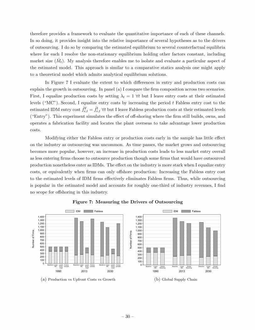
therefore provides a framework to evaluate the quantitative importance of each of these channels.
In so doing, it provides insight into the relative importance of several hypotheses as to the drivers
of outsourcing. I do so by comparing the estimated equilibrium to several counterfactual equilibria
where for each I resolve the non-stationary equilibrium holding other factors constant, including
market size (Mt). My analysis therefore enables me to isolate and evaluate a particular aspect of
the estimated model. This approach is similar to a comparative statics analysis one might apply
to a theoretical model which admits analytical equilibrium solutions.
In Figure 7 I evaluate the extent to which differences in entry and production costs can
explain the growth in outsourcing. In panel (a) I compare the firm composition across two scenarios.
First, I equalize production costs by setting λt = 1 ∀t but I leave entry costs at their estimated
levels (“MC”). Second, I equalize entry costs by increasing the period t Fabless entry cost to the
estimated IDM entry cost fFe,t = f I
e,t ∀t but I leave Fabless production costs at their estimated levels
(“Entry”). This experiment simulates the effect of off-shoring where the firm still builds, owns, and
operates a fabrication facility and locates the plant overseas to take advantage lower production
costs.
Modifying either the Fabless entry or production costs early in the sample has little effect
on the industry as outsourcing was uncommon. As time passes, the market grows and outsourcing
becomes more popular, however, an increase in production costs leads to less market entry overall
as less entering firms choose to outsource production though some firms that would have outsourced
production nonetheless enter as IDMs. The effect on the industry is more stark when I equalize entry
costs, or equivalently when firms can only offshore production: Increasing the Fabless entry cost
to the estimated levels of IDM firms effectively eliminates Fabless firms. Thus, while outsourcing
is popular in the estimated model and accounts for roughly one-third of industry revenues, I find
no scope for offshoring in this industry.
Figure 7: Measuring the Drivers of Outsourcing
0100200300400500600700800900
1,0001,1001,2001,3001,400
Num
ber o
f Firm
s
1990 2013 2030
Baseline LowerMC
LowerEntryCost
FutureGrowth
Baseline LowerMC
LowerEntryCost
FutureGrowth
Baseline LowerMC
LowerEntryCost
FutureGrowth
IDM Fabless
(a) Production vs Upfront Costs vs Growth
0100200300400500600700800900
1,0001,1001,2001,3001,400
Num
ber o
f Firm
s
1990 2013 2030
Baseline LowerMC
GlobalSourcing
Baseline LowerMC
GlobalSourcing
Baseline LowerMC
GlobalSourcing
IDM Fabless
(b) Global Supply Chain
– 30 –

In panel b, I evaluate the role of global supply chains on composition of firms in this
industry. I do so by adjusting the production cost advantage afforded to Fabless firms to eliminate
the gains of overseas production found in Table III.24 The results indicate that outsourcing does
decrease when we remove overseas markets but the effect is not dramatic. Thus, outsourcing in
this industry is not solely motivated by factors which drive global supply chains such as reductions
in transportation costs or import tariffs.
5.1 Measuring the Impact of Venture Capital
Thus far I have treated the estimated entry costs as a primitive while in reality they represent
a variety of inputs required to establish a firm, including financing where venture capital has
traditionally played a significant role. Interestingly, growth of the semiconductor industry, and
particularly of the Fabless business model, is closely-aligned with growth of the venture capital
industry as the latter enables financing and operational expertise to start-ups.
In Figure 8 I evaluate how changes in the venture capital industry could have impacted
the semiconductor industry. I do so via the interest rate charged to the prospective entrepreneur
thinking of starting either an IDM or Fabless firm in period t where I assume the entry costs can
be decomposed into a principal amount required to start a IDM or Fabless firm and a “Financing
Charge”:
f je,t = f j
e,t × (1 + “Financing Charge”) ,
where the left-hand side is the estimated entry cost incurred by period t IDM or Fabless firms. The
“Financing Charge” is simply a markup required to secure financing though it may also reflect any
additional costs required to find funding.
Under the estimated model, I decompose the estimated entry costs into actual capital
expenditure (i.e., money spent on buildings and equipment) and interest expense where I assume
a 20% interest rate – a rate of return consistent with venture capital benchmarks. I then simulate
an increase in the entry costs of firms (both IDM and Fabless) by increasing the interest rate to
30% and 40% which increases entry costs.
An increase in the financing rate decreases the number of firms in the industry significantly
indicating the industry’s sensitivity to changes in start-up costs and reliance on financing channels
such as venture capital (panel a). While the increased financing cost decreased firm entry and
consequently the equilibrium number of firms in the industry, the fact that both IDM and Fabless
firms are financed through venture capital had little impact on the changing composition of firms
(panel b). Interestingly, at financing costs the growth of Fabless firms, as a percent of total, is
24Recall that in Table III I used to the detailed wafer pricing data to show that outsourcing production to anoverseas firm (e.g., Taiwan Semiconductor) represented a 26.95% reduction in cost relative to outsourcing to a USfirm. In columns marked “Domestic” I resolve the non-stationary equilibrium when Fabless production costs areλt = λt/(1− 0.2695).
– 31 –

Figure 8: The Role of Venture Capital Funding
End of Sample (2013)
0100200300400500600700800900
1,0001,1001,2001,3001,4001,500
Tota
l Num
ber o
f Firm
s in
the
Indu
stry
1990 1995 2000 2005 2010 2015 2020 2025 2030
Year
20% 30% 40%
(a) Number of Firms
End of Sample (2013)
0
10
20
30
40
50
60
70
80
90
100
Shar
e of
Firm
s w
hich
are
IDM
1990 1995 2000 2005 2010 2015 2020 2025 2030
Year
20% 30% 40%
(b) IDM Share
slower than in the estimated model at the beginning of the 1990s but accelerates at the end of the
1990s to reach the same steady state level by 2000.
6 Conclusion
In this paper I addressed the equilibrium effects of outsourcing on the evolution of the semiconductor
industry. I did so by developing a dynamic oligopoly model of innovation in which firms strategically
outsource production overseas and invest to increase the quality of their product. To account for
exogenous market growth I consider firm strategies which vary over time as the market grows
and transitions between steady-states. I then estimated the model using detailed data from the
semiconductor industry – an industry in which outsourcing has become a significant business model.
The estimated model replicates moments in the data well and generates reasonable and statistically
significant parameter values.
I show that growth of outsourcing was largely due to the ability of firms to avoid the
large cost of building a fabrication facility rather than lower production costs due to economies
of scale from third-party facilities. I also find that the industry’s evolution is sensitive to changes
in the venture capital industry which would have impacted financing rates and therefore capital
expenditure costs. These results indicate that outsourcing amounted to a new financial technology
which decreased entry costs and enabled entry of smaller companies. Increased entry of Fabless
firms ultimately led to increased competition for the traditional, vertically-integrated IDMs leading
to less profits for these firms and ultimately less entry.
While the model captures many of the important characteristics of the industry, there are
potential avenues for improvement. Including research spillovers as in Goettler and Gordon (2011),
endogenous research effort, and accounting for mergers are all promising avenues for future research.
– 32 –

References
Antras, P., T. C. Fort, and F. Tintelnot (2017): “The Margins of Global Sourcing: Theoryand Evidence from U.S. Firms,” American Economic Review, 107(9), 2514–64.
Atalay, E., A. Hortacsu, M. J. Li, and C. Syverson (2017): “How Wide Is the FirmBorder?,” Working Paper 23777, National Bureau of Economic Research.
Atkeson, A., and A. T. Burstein (2010): “Innovation, Firm Dynamics, and InternationalTrade,” Journal of Political Economy, 118(3), 433–484.
Bajari, P., C. L. Benkard, and J. Levin (2007): “Estimating Dynamic Models of ImperfectCompetition,” Econometrica, 75(5), 1331–1370.
Bergstrand, J., M. Larch, and Y. Yotov (2015): “Economic integration agreements, bordereffects, and distance elasticities in the gravity equation,” European Economic Review, 78,307–327.
Berry, S. (1994): “Estimating Discrete-Choice Models of Product Differentiation,” RAND Journalof Economics, 25, 242–262.
Berry, S., and G. Compiani (2017): “An Instrumental Variables Approach to Dynamic Models,”mimeo.
Besanko, D., M. Perry, and R. Spady (1990): “The Logit Model of Monopolistic Competition:Brand Diversity,” The Journal of Industrial Economics, 38, 397–415.
Caplin, A., and B. Nalebuff (1991): “Aggregation and Imperfect Competition: On the Exis-tence of Equilibrium,” Econometrica, 59, 1–23.
Collard–Wexler, A. (2013): “Demand Fluctuations in the Ready-Mix Concrete Industry,”Econometrica, 81(3), 1003–1037.
Davis, S., J. Haltiwanger, R. Jarmin, and J. Miranda (2007): “Volatility and Dispersion inBusiness Growth Rates: Publicly Traded versus Privately Held Firms,” in NBER Macroe-conomics Annual 2006, Volume 21, pp. 107–180. National Bureau of Economic Research,Inc.
Dickstein, M. J., and E. Morales (2018): “What do Exporters Know?*,” The QuarterlyJournal of Economics, 133(4), 1753–1801.
Dube, J., J. T. Fox, and C. Su (2012): “Improving the Numerical Performance of Static andDynamic Aggregate Discrete Choice Random Coefficients Demand Estimation,” Economet-rica, 80(5), 2231–2267.
Ericson, R., and A. Pakes (1995): “Markov-perfect industry dynamics: a framework forempirical work,” Review of Economic Studies, 62(1), 53–82.
Fershtman, C., and A. Pakes (2012): “Dynamic Games with Asymmetric Information: AFramework for Empirical Work,” Quarterly Journal of Economics, 127(4), 1611–1661.
Goettler, R. L., and B. R. Gordon (2011): “Does AMD Spur Intel to Innovate More?,”Journal of Political Economy, 119(6), 1141 – 1200.
– 33 –

Gourieroux, C., A. Monfort, and E. Renault (1993): “Indirect Inference,” Journal ofApplied Econometrics, 8, S85–S118.
Hall, B. H., A. B. Jaffe, and M. Trajtenberg (2001): “The NBER Patent Citation DataFile: Lessons, Insights and Methodological Tools,” Working Paper 8498, National Bureauof Economic Research.
Hall, B. H., and R. H. Ziedonis (2001): “The Patent Paradox Revisited: An Empirical Study ofPatenting in the U.S. Semiconductor Industry, 1979-1995,” RAND Journal of Economics,32(1), 101–28.
Hall, G., and J. Rust (2003): “Simulated Minimum Distance Estimation of a Model of OptimalCommodity Price Speculation with Endogenously Sampled Prices,” mimeo.
Hansen, L. P. (1982): “Large Sample Properties of Generalized Method of Moments Estimators,”Econometrica, 50, 1029–1054.
Hummels, D. (2007): “Transportation Costs and International Trade in the Second Era ofGlobalization,” Journal of Economic Perspectives, 21(3), 131–154.
Hummels, D., J. Ishii, and K.-M. Yi (2001): “The nature and growth of vertical specializationin world trade,” Journal of International Economics, 54(1), 75–96.
Hunt, R. (1996): “The Value of R&D in the U.S. Semiconductor Industry: What Happened inthe 1980s?,” mimeo.
Ifrach, B., and G. Y. Weintraub (2016): “A Framework for Dynamic Oligopoly in Concen-trated Industries,” The Review of Economic Studies, 84(3), 1106–1150.
Igami, M. (2017): “Estimating the Innovator’s Dilemma: Structural Analysis of Creative Destruc-tion in the Hard Disk Drive Industry, 1981–1998,” Journal of Political Economy, 125(3),798–847.
(2018): “Industry Dynamics of Offshoring: The Case of Hard Disk Drives,” AmericanEconomic Journal: Microeconomics, 10(1), 67–101.
Jeon, J. (2019): “Learning and Investment under Demand Uncertainty in Container Shipping,”mimeo.
Johnson, R. C., and G. Noguera (2017): “A Portrait of Trade in Value-Added over FourDecades,” The Review of Economics and Statistics, 99(5), 896–911.
Kortum, S., and J. Lerner (1998): “Stronger protection or technological revolution: what isbehind the recent surge in patenting?,” Carnegie-Rochester Conference Series on PublicPolicy, 48(1), 247–304.
Lancaster, K. J. (1966): “A New Approach to Consumer Theory,” Journal of Political Economy,74.
Levin, R. C. (1982): “The Semiconductor Industry,” in Government and Technical Progress: ACross-Industry Analysis (Pergamon. Press.
Lucas, R. E. (1978): “On the Size Distribution of Business Firms,” The Bell Journal of Economics,9(2), 508–523.
– 34 –

Maskin, E., and J. Tirole (1988): “A Theory of Dynamic Oligopoly, I: Overview and QuantityCompetition with Large Fixed Costs,” Econometrica, 56(3), 549–69.
Pakes, A., and D. Pollard (1989): “Simulation and the Asymptotics of Optimization Estima-tors,” Econometrica, 57(5), 1027–1057.
Ryan, S. P. (2012): “The Costs of Environmental Regulation in a Concentrated Industry,”Econometrica, 80(3), 1019–1061.
Seim, K. (2006): “An Empirical Model of Firm Entry with Endogenous Product-Type Choices,”The RAND Journal of Economics, 37(3), 619–640.
Standard & Poor’s Compustat (1980-2014): http://wrds.wharton.upenn.edu/.
Taylor, C., and Z. Silbertson (1973): The Economic Impact of the Patent System: A Studyof the British Experience. New York: Cambridge University Press.
Tilton, J. E. (1971): International diffusion of technology; the case of semiconductors [by] JohnE. Tilton. Brookings Institution Washington,.
von Hippel, E. (1988): The Sources of Innovation. Oxford University Press.
Weyl, E., and M. Fabinger (2013): “Pass-Through as an Economic Tool: Principles of Incidenceunder Imperfect Competition,” Journal of Political Economy, 121, 528–583.
– 35 –

A Other Results
Figure 9: A Growing Market (Mt)
0255075
100125150175200225250275300325350375
Mar
ket S
ize
(M)
1990
1992
1994
1996
1998
2000
2002
2004
2006
2008
2010
2012
2014
Year
Market Size (M)
Table VI: The Foundry Market
Company Type Country Revenue ($M) % of Total
1. TSMC Pure-play Taiwan 13,332 46.67
2. UMC Pure-play Taiwan 3,824 13.39
3. GlobalFoundries Pure-play United States 3,520 12.32
4. SMIC Pure-play China 1,554 5.44
5. Dongbu HiTek Pure-play South Korea 512 1.79
6. TowerJazz Pure-play Israel 509 1.78
7. Vanguard (VIS) Pure-play Taiwan 505 1.77
8. IBM IDM United States 500 1.75
9. MagnaChip IDM South Korea 410 1.44
10. Samsung Semiconductor IDM South Korea 390 1.37
Others - - 3,510 12.29
Total - - 28,566 100.00
Source: Gartner. “Pure-play” foundries are fabrication plants in which all production is of chips designed
by other companies. “IDM” foundries are internal fabrication facilities. In 2015 IBM exited the foundry
business and sold its operations to GlobalFoundries.
– 36 –