Outline:

1 Witsenhausen’s counterexample.

2 Signaling strategies.

3 The infinite-length Witsenhausen counterexample.

4 The finite-dimensional problem.

Pulkit Grover, Anant Sahai and Se Yong Park.

“The finite-dimensional Witsenhausen Counterexample”Control over Communication Channels (ConCom), 2009.

Slides available: www.eecs.berkeley.edu/∼pulkit/ConCom09Slides.pdfThis Handout: . . . /∼pulkit/ConCom09Handout.pdfFurther discussion and references can be found in the paper.

1 The Witsenhausen counterexample

min{

k2E

[

u12]

+ E[

x22]}

.

Encoder ++ Decoder

E[

u12]

≤ P

x0 ∼ N (0, σ2

0) w ∼ N (0, 1)

x1u1u2x̂1=

min E[

(x1 − x̂1)2]

x1 − x̂1

The Witsenhausen counterexample [Witsenhausen’68] is adistributed Linear-Quadratic-Gaussian problem for whichnonlinear control laws outperform the optimal linear con-trol law. The optimal control law is still elusive — and thenon-Gaussian relaxation of the problem is known to be NP-complete [Papadimitriou and Tsitsiklis ’86].

The counterexample has an implicit channel that makes ithard. The first controller modifies the initial state and at-tempts to communicate the modified state to the second con-troller through a noisy channel. Solving the problem of min-imizing MMSE error in estimating x̂1 with an average powerconstrained u1 is an equivalent formulation.

2 Signaling strategies over the implicit channel

-

2

-

1

0 2 x0

u1

x1

1

[Mitter and Sahai, 99] used quantization-based signaling strategiesthat beat the optimal linear strategy by a factor that can be arbi-trarily large, depending on the problem parameters. However, itwas unclear if there exists a strategy that beats quantization-basedstrategies also by an arbitrarily large factor.

3 Vector version of Witsenhausen’s counterexample

E ++ D x̂1

x1u1

E[

‖u1‖2]

≤ mP

x0 ∼ N (0, σ2

0I) w ∼ N (0, I)

min1

m

E[‖x1 − x̂1‖

2]

x1 − x̂1

The counterexample can be extended to a vector problem ofvector length m [Ho, Kastner and Wong ’78]. The asymptot-ically infinite length extension offers simplification becauseit allows us to avoid the complications associated with thegeometry of finite-dimensional spaces.

3.1 Vector quantization (VQ)

Vector quantization

points

shell oftypical initial states

m(s - P)20

initial state

ms20

x0

x1

u1

Provided the number of quantization points is sufficiently small,they can be decoded correctly at the second controller. Asymp-totic cost is k2σ2

w and 0 for the first and the second stage respec-tively.

3.2 Our lower bound

Witsenhausen’s lower bounding technique does not extendto the vector case (and further, is loose for the scalar case).We provide the following new lower bound to the optimalcosts which is valid for all vector lengths m ≥ 1,

C̄min ≥ infP≥0

k2P +((√

κ(P ) −√

P )+)2

,

where κ(P ) =σ2

0σ2

w

σ2

0+2σ0

√P+P+σ2

w

, where σ2w = 1 is the obser-

vation noise variance. This bound is tighter than Witsen-hausen’s bound for the scalar problem in some cases.

The ratio of optimal linear costs to the lower bound increasesto infinity in the small-k large-σ regime.

−10−5

05

10

−20−10

010

20

1

2

3

4

5

log10

(k)log10

(σ02)

Rat

io

Ratio of upper and lower bounds usingthe JSCC strategy and two linear strategies

The ratio of our upper bound (obtained by using the vectorquantization strategy and two linear schemes of zero-inputand zero-forcing) and our lower bound is bounded by 4.45for the VQ strategy. Analytically, we can show that theratio is bounded by 11. Observe that the ratio is quite closeto 1 for “most” values of k and σ2

0 .

3.3 Improved ratio using Dirty-Paper Coding (DPC) based strategies

u1

x0

αx0

x0

u1

x1

αx0

√

m(P + α2σ

2

0)

An interpretation of the "slopey"

quantization strategies of [Baglietto et al]

The exact same sequence of steps yields

the DPC-based strategy!

!!

!"

#

"

!"!$

#$

"$

$%"

$%!

$%&

$%'

"

log10(k)

log10(!0

2)

Ratio

()*+,-,.-/0012-)34-5,612-7,/348-/8+39*:1-;,<7+3)*+,3-=>?@-A-5+31)2B-8*2)*19C

!0

2 = 0.618

Ratio of costs attained by combination (DPC+linear) strategy

and our lower bound

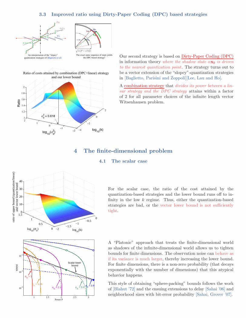
Our second strategy is based on Dirty-Paper Coding (DPC)in information theory where the shadow state αx0 is drivento the nearest quantization point . The strategy turns out tobe a vector extension of the “slopey”-quantization strategiesin [Baglietto, Parisini and Zoppoli][Lee, Lau and Ho].

A combination strategy that divides its power between a lin-ear strategy and the DPC strategy attains within a factorof 2 for all parameter choices of the infinite length vectorWitsenhausen problem.

4 The finite-dimensional problem

4.1 The scalar case

−2−1.5

−1−0.5

0

0

0.5

1

1.50

10

20

30

40

log10

(k)log10

(σ0)

ratio

of u

pper

bou

nd (

quan

tizat

ion/

linea

r)an

d ve

ctor

low

er b

ound

For the scalar case, the ratio of the cost attained by thequantization-based strategies and the lower bound runs off to in-finity in the low k regime. Thus, either the quantization-basedstrategies are bad, or the vector lower bound is not sufficientlytight.

1 1.5 2 2.5 3

10−6

10−4

10−2

Power P

MM

SE

Scalar lower bound

σG

= 1

σG

= 1.25σ

G = 2.1 σ

G = 3.0

σG

= 3.9

A “Platonic” approach that treats the finite-dimensional worldas shadows of the infinite-dimensional world allows us to tightenbounds for finite dimensions. The observation noise can behave asif its variance is much larger, thereby increasing the lower bound.For finite dimensions, there is a non-zero probability (that decaysexponentially with the number of dimensions) that this atypicalbehavior happens.

This style of obtaining “sphere-packing” bounds follows the workof [Blahut ’72] and the ensuing extensions to delay [Sahai ’06] andneighborhood sizes with bit-error probability [Sahai, Grover ’07].

−2

−1

0

00.20.40.60.812

4

6

8

log10

(k)log10

(σ0)

ratio

of u

pper

and

low

er b

ound

s

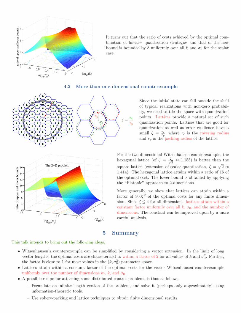
It turns out that the ratio of costs achieved by the optimal com-bination of linear+ quantization strategies and that of the newbound is bounded by 8 uniformly over all k and σ0 for the scalarcase.

4.2 More than one dimensional counterexample

x0

rc

rp

ζ =

rc

rp

rc

Since the initial state can fall outside the shellof typical realizations with non-zero probabil-ity, we need to tile the space with quantizationpoints. Lattices provide a natural set of suchquantization points. Lattices that are good forquantization as well as error resilience have asmall ζ = rc

rp, where rc is the covering radius

and rp is the packing radius of the lattice.

−2

−1

0

00.5

11.5

2

4

6

8

10

12

14

16

log10

(k)log

10(σ

0)

ratio

of u

pper

and

low

er b

ound

s

The 2−D problem

For the two-dimensional Witsenhausen counterexample, thehexagonal lattice (of ζ = 2√

3≈ 1.155) is better than the

square lattice (extension of scalar-quantization, ζ =√

2 ≈1.414). The hexagonal lattice attains within a ratio of 15 ofthe optimal cost. The lower bound is obtained by applyingthe “Platonic” approach to 2-dimensions.

More generally, we show that lattices can attain within afactor of 300ζ2 of the optimal costs for any finite dimen-sion. Since ζ ≤ 4 for all dimensions, lattices attain within aconstant factor uniformly over all k, σ0, and the number ofdimensions. The constant can be improved upon by a morecareful analysis.

5 Summary

This talk intends to bring out the following ideas:

• Witsenhausen’s counterexample can be simplified by considering a vector extension. In the limit of longvector lengths, the optimal costs are characterized to within a factor of 2 for all values of k and σ2

0. Further,the factor is close to 1 for most values in the (k, σ2

0) parameter space.

• Lattices attain within a constant factor of the optimal costs for the vector Witsenhausen counterexampleuniformly over the number of dimensions m, k, and σ0.

• A possible recipe for attacking some distributed control problems is thus as follows:

– Formulate an infinite length version of the problem, and solve it (perhaps only approximately) usinginformation-theoretic tools.

– Use sphere-packing and lattice techniques to obtain finite dimensional results.