Out of site out of mind: Quantifying the long-term off-site economic impacts of land degradation in Kenya

By

Ephraim Nkonya1, Patrick Gicheru2, Johannes Woelcke3, Barrack Okoba2,

Daniel Kilambya2, and Louis N. Gachimbi2,

1 International Food Policy Research Institute (IFPRI) 2033 K Street N.W., Washington D.C. 2006, USA

2 Kenya Agricultural Research Institute (KARI)

P.O. Box 14733, Nairobi Kenya

3 World Bank 1818 H Street, Washington D.C. 20433 USA

Selected paper prepared for presentation at the American Agricultural Economics Association Annual Meeting, Long Beach, California, July 23-26, 2006.

Copyright by Ephraim Nkonya, Patrick Gicheru, Johannes Woelcke, Barrack Okoba, Daniel Kilambya, and Louis N. Gachimbi. All rights reserved. Readers may make verbatim copies of this document for non-commercial purposes by any means, provided that this copyright notice appears on all such copies.

Land degradation in sub-Saharan Africa (SSA) is a serious problem that is threatening

livelihoods of the poor who depend on agriculture. The problem also poses a challenge to

economic development since economies of most countries in the region are based on agriculture.

Land degradation also leads to sedimentation of surface water bodies, runoff and flooding and

other off-site effects (Pagiola, 1999; Scherr and Yadav, 1996; Schroeder, 1993; Unruh, et al.,

1993) at local and national level. At global scale, land degradation has been identified as one of

the factors that contribute to climate change and loss of biodiversity. Contribution of land

degradation to climate change mainly results from emission of Greenhouse Gases (GHG) as a

result of bush and crop residue burning and other processes that lead to disruption of the carbon

cycle. Degraded land also loses vegetative cover that absorbs the shortwave radiation, leading to

global warming (Glasdottir and Stocking 2005). Another effect of changes in vegetative cover is

a change in albedo (reflectivity), which changes the absorption of energy. Albedo may have

positive or negative effects on warming, depending on the albedo of what replaces the

vegetation.

Soil erosion and soil nutrient depletion are the major forms of land degradation in SSA

(Pieri, 1989; Oldeman, 1994; Oldeman, et al., 1991; Voortman, et al., 2000). In addition to

contributing to fall in agricultural productivity and the consequent food and nutrition insecurity,

soil nutrient depletion and erosion could also contribute to deforestation and loss of biodiversity

since farmers may be forced to abandon nutrient-starved soils and cultivate more marginal areas

such as hillsides and rainforests. Loss of biodiversity and poor water quality in turn could

contribute to increase in pests and diseases (Scherr, 2000).

Given the real and potential on-farm and off-site negative impacts of land degradation

discussed above, governments in SSA and their development partners have been designing

1

strategies and policies to address the problem as part of their poverty reduction and

environmental conservation efforts. This study was conducted with the purpose of determining

the on-farm and off-farm economic impacts of land degradation in central Kenya.

Accounting for off-site effects of land degradation

There are many types of land degradation with equally numerous off-site effects. We will

therefore focus on only two, namely soil erosion and degradation of vegetation on crop plots and

their potential on-farm and off-site impacts. We analyze the offsite effects that we can attribute

to land degradation unambiguously and those which we were able to get the costs and benefits

data. We quantify the offsite impacts related to sedimentation and how it affects the cost of

potable water production. We also analyze the amount of carbon stored in the planted trees,

shrubs and grasses, and soil carbon saved due to soil and water conservation or lost due to soil

erosion and other channels. Our study is based on a case study of Sasumua water treatment plant

located in the Kinale/Kikuyu watershed, which is in the central provinces of Kenya.1 We

consider two scenarios, namely farmer practices that use what we call Sustainable Land

Management (SLM) and those who do not practice SLM. The SLM practices considered in this

study include:

(i) Agroforestry to help control soil erosion, increase carbon stock, improve soil fertility and

other agroforestry benefits (see Sanchez, et al., 1997).

(ii) Application of organic and inorganic fertilizer and incorporation of crop residues

(iii) SWC practices to control soil erosion and to conserve moisture and water.

2

Though these technologies are highly interrelated, they are separated in this research to

emphasize their importance. The SLM practices are assumed to address the offsite effects of soil

erosion and degradation of vegetation.

We use the common indicators for economic returns, i.e. Net Present Value (NPV) and

the Internal Rate of Return (IRR) to determine whether the SLM practices are profitable from the

social perspective. The social Cost-Benefit Analysis (CBA) takes into account the on-farm and

off-farm costs and benefits at farm level and at society (community, district, national, regional

and global) level. The social NPV will be compared with the private NPV to reflect the benefits

and costs that farmers realize when they ignore the off-site effects of production. Hence,

comparing the social and private NPV will reflect the impacts of externalities of agricultural

production on profit.

We do the social CBA by considering the market failures or policy-induced distortions

might distort price signals perceived by agricultural producers; and externalities of land

degradation, which might impose costs or benefits on the society.2 Although the importance of

off-site effects of land degradation is widely recognized, most studies focus exclusively on on-

farm effects. This is mainly due to difficulties encountered in quantifying and valuing off-site

effects. This study quantified the off-site effects of land degradation using data obtained from the

Kinale/Kikuyu watershed in the central provinces of Kenya. We assess the cost and benefit with

and without SLM practices over a 50 year period. Using a discount rate of 10% (see Pagiola,

1996),3 the NPV of the costs and benefits is computed with and without soil fertility

management, agroforestry and SWC structures, which are the three main components of the

SLM considered in this study. If soil erosion is the major form of land degradation in the study

area, the effects of continued erosion on agricultural productivity is estimated Using the returns

3

to the investment, which are obtained by taking the difference between the streams of discounted

costs and benefits, with and without the adoption of the soil conservation practices. This

valuation technique is commonly called the ‘change of productivity approach’.4 This approach

will be used in this study. The approach estimates only the discounted returns to the specific

conservation measure being examined.

Due to data availability problems, a simple, flexible and less data intensive model was

used to determine the soil loss due to erosion. This model is the Revised Universal Soil Loss

Equation (RUSLE) (Renard, et al., 1991). The RUSLE model relates soil loss from a field to the

climate, type of soil, topography, and management variables as follows:

A = RKLSCP

Where A is the mean annual soil loss (metric tons per hectare), R is the rainfall erosivity index,

K is the soil erosivity index, L is the slope length, S is the slope steepness, C is the crop factor,

and P is the conservation practice factor.

The weakness of this approach is related to the fact that the crop yield response to soil

erosion over time is complex hence controlling for all factors is difficult (Enters, 1998).

Additionally, most soil erosion data are exaggerated since they are based on small plots and then

extrapolated to larger areas such as a catchment, district, region, etc (Glasdottir and Stocking,

2005; Koning and Smaling, 2005). Even though the RUSLE results don’t account for

redeposition, they give a reasonable order of magnitude estimate of on-site costs of erosion from

highlands, since these areas are more sources than recipients of erosion. However, due to its

parsimonious data requirement and simplicity, RUSLE remains one of the most widely used soil

erosion prediction model and has been used in Kenya and many other SSA countries.

4

The quantity of soil eroded is related to the corresponding crop yield in order to

determine the loss of crop productivity due to soil erosion. Since crop yield is determined by

many factors, the best estimate is obtainable under experimental conditions, in which most of

such factors are controlled. Once the functional relationship between crop yield and soil erosion

is determined, the value of crop yield loss due to erosion is computed and used to determine the

benefits and costs of investing in controlling soil erosion. Likewise, the value of loss of crop

productivity due to soil fertility mining is determined using data from a long-term soil fertility

experiment conducted in Kabete, Kenya. This value is also used to determine the benefits and

costs of practicing soil fertility management technologies.

The impact of deforestation and reduction of carbon stock in general is estimated after

determining the amount of lost carbon using various silvicultural methods. A value is then

imputed on the quantity of carbon lost. Land degradation is often correlated with increased soil

carbon dioxide emissions and a reduced ability to store carbon. However, as Pagiola (1999)

notes, the links between land degradation and carbon dioxide emission are numerous and

complex and hence difficult to quantify. Some actions which cause land degradation can increase

carbon emissions directly, e.g. bush and crop burning. Some forms of degradation reduce soil

carbon, since erosion carries away Soil Organic Matter (SOM). However, this does not

necessarily lead to increased emissions, because much of the carbon carried away by erosion

may be deposited under conditions where it may be well preserved (e.g. in riverbeds and

reservoirs). Land degradation also affects the soil carbon cycle. Lower production of crops and

pasture due to degradation will result in lower carbon inputs in subsequent periods. Due to these

complex relations the effect of land degradation on soil carbon sequestration is difficult to

quantify. Hence, we will use coefficients generated by previous studies and adapt them to the

5

Kenyan conditions. Once carbon sequestration (and emission) has been quantified for both with-

and without SLM scenarios a value will be attached to the – most likely – reduced emissions.

Other studies usually value the CO2 emission reduction at US$ 3-4 per ton of carbon.

Analytical methods and data

Analytical methods

We quantify the impact of each of the three SLM practices and assess the profitability of

adopting them. We begin by specifying the CBA model (profit function) and then specify the

biophysical relationships that attribute the impact of SLM practices on agricultural productivity.

Equation (1) and (2) specify the profit of adopting or not adopting the SLM practices:

Profit with SLM

(1) ( )c c c ct t t t tY P Zπ λ= − ±

Where: ctπ = Profit with SLM practices in year t

c = Crop yield with SLM practices in year t tY

Pt = Social price of output in year t

ctZ = Social cost of production of one unit of c

tY

ctλ = Off-site costs/benefits with SLM practices per unit produced in year t

Profit without SLM

(2) ( )d d d dt t t t tY P Zπ λ= − ±

Where: dtπ = Profit without SLM practices in year t

6

= Crop yield without SLM practices in year t dtY

dtZ = Cost of production of one unit of d

tY

dtλ = Off-site costs/benefits without SLM practices per unit produced in year t

The social NPV (NPVs) of adopting SLM practices is therefore given by

(3) 0

( )T

t c dt t

t

sNPV ρ π π=

= −∑

Where T = farmers’ planning horizon

ρt = 11

t

r⎛ ⎞⎜ +⎝ ⎠

⎟ = farmers’ discount factor, where r is the farmer’s private discount rate

Farmers will find it profitable to adopt SLM practices if NPV>0. However, farmers’

decision to adopt SLM practices does not take into account the off-site costs and benefits that

result from adoption or non-adoption of SLM practices. This also doesn’t account for risk, credit

constraints, size and irreversibility of investment. The literature on these issues also establishes

that a positive NPV may be far from sufficient to induce investment (e.g., Pender 1996; Dixit

and Pindyck 1994; Fafchamps and Pender 1997).

Following its definition, the IRR is given by:

(4) 0

( )1 0

1

tTc dt t

t

NPVIRR

π π=

= −⎛ ⎞ =⎜ ⎟+⎝ ⎠∑ :

The greater the IRR, the higher the rate of returns to investment.

7

The first step to computing equations (1) through (3) is to find how crop yields

( and ) are affected by the SLM practices, namely, soil fertility management, agroforestry

and SWC structures. Ideally, we need data from an experiment that included all three SLM types

and conducted over many years to capture the long-term biophysical changes and the

corresponding crop yield changes. To the best of our knowledge, there is no such experiment in

SSA or other countries with biophysical characteristics similar to Kenya. However, there are

three sets of long-term and short-term experiments conducted in Kenya that investigated

separately the response of crop yield to (i) organic and inorganic fertilizer and crop residue

management, (ii) SWC structures and (iii) agroforestry (Calliandra and Napier grass)

treatments.

ctY d

tY

5 We will use the results of these experiments to establish the relationship between

crop yield and the three SLM practices.

To simplify the modeling approach, we assume that crop yield is affected by soil

moisture, soil quality (chemical and biophysical characteristics such as soil nutrients present in

the soil, bulk density), and topsoil depth. In low external input agriculture -- such as the study

area, agronomists use topsoil depth to determine SOM and soil fertility in general (Koning and

Smaling, 2005; Mantel and van Engelen, 2000; Nkonya, 1999).

(5) Crop yield = f(soil moisture, soil quality, topsoil depth, εt)

Where εt is a random error.

Topsoil depth (x) may not be a good indicator of soil quality since two soils of the same topsoil

depth may have quite different SOM levels due to its different uses. Hence we introduce the soil

quality term to account for such possibility. All three SLM practices affect soil quality and

topsoil depth. There are many attributes of soil quality that are not easy to model. Holding land

8

management and biophysical conditions constant, these attributes will change over time if the

farmer practices continuous cultivation. For example, in the long-term Kabete soil fertility trial,

crop yield under continuous cultivation decreases largely due to decline in SOM over time even

in treatments receiving the highest rates of organic and inorganic fertilizer (Nandwa and

Bekunda, 1998).6 This implies inorganic and organic fertilizers cannot replenish some nutrients

required for increasing or maintaining crop productivity. Hence, holding land management and

most biophysical conditions constant,7 SOM will be strongly correlated with the number of years

of continuous cultivation. Hence we assume that under controlled long-term soil fertility

experimental conditions, the change in crop yield over years will largely be attributable to

changes in the SOM. However, since researchers of the soil fertility experiments in Kenya did

not control for rainfall changes (e.g., using irrigation), we need to control for rainfall amount.

Controlling for soil depth (through effective control of soil erosion), the cumulative soil erosion,

xt = 0, hence the empirical model representing the impact of soil quality on crop yield with SLM

practices over years is:

(6) = f(rainfall, yearly trend of changes of soil quality, εctY t)

The impact of rainfall on crop yield is likely to be positive exponential since crop yield response

to rainfall will be very strong under moisture stress conditions but it will taper off when moisture

stress decreases. Eventually, crop yield will not respond to rainfall when soil moisture reaches a

certain threshold.

Exploratory investigation of the Kenyan long-term soil fertility trial showed that the

maize crop yield declined exponentially over years.8 Hence equation (6) is explicitly specified in

the following model that also shows the expected signs:

9

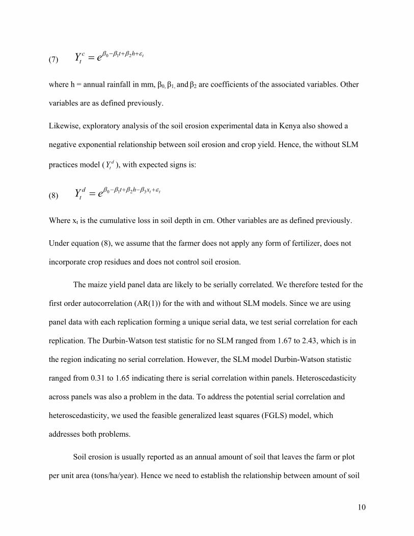
(7) 0 1 2 tt hctY eβ β β ε− + +=

where h = annual rainfall in mm, β0, β1, and β2 are coefficients of the associated variables. Other

variables are as defined previously.

Likewise, exploratory analysis of the soil erosion experimental data in Kenya also showed a

negative exponential relationship between soil erosion and crop yield. Hence, the without SLM

practices model ( ), with expected signs is: dtY

(8) 0 1 2 3 t tt h xdtY eβ β β β ε− + − +=

Where xt is the cumulative loss in soil depth in cm. Other variables are as defined previously.

Under equation (8), we assume that the farmer does not apply any form of fertilizer, does not

incorporate crop residues and does not control soil erosion.

The maize yield panel data are likely to be serially correlated. We therefore tested for the

first order autocorrelation (AR(1)) for the with and without SLM models. Since we are using

panel data with each replication forming a unique serial data, we test serial correlation for each

replication. The Durbin-Watson test statistic for no SLM ranged from 1.67 to 2.43, which is in

the region indicating no serial correlation. However, the SLM model Durbin-Watson statistic

ranged from 0.31 to 1.65 indicating there is serial correlation within panels. Heteroscedasticity

across panels was also a problem in the data. To address the potential serial correlation and

heteroscedasticity, we used the feasible generalized least squares (FGLS) model, which

addresses both problems.

Soil erosion is usually reported as an annual amount of soil that leaves the farm or plot

per unit area (tons/ha/year). Hence we need to establish the relationship between amount of soil

10

lost per unit area per year and the corresponding loss of depth of topsoil. This relationship was

established in Kenya by Mantel and van Engelen (2000) as follows:

(9) 4 * *10010E Tx

B⎛ ⎞= ⎜ ⎟⎝ ⎠

Where: x = topsoil loss (cm)

E = Soil erosion risk in kg ha-1yr-1.

T = number of years in the planning horizon. In this study we seek to understand the loss

of topsoil depth in 50 years.

B = bulk density of topsoil in kg m-3.

Since agroforestry is one of the technologies for controlling soil erosion and improving of soil

quality, it is implicitly incorporated into equation (7) and (8). However, its impact will be

explicitly specified when estimating equations (1) through (3). Details on how we treated

agroforestry are given in the next (data) section.

Data

The data section describes how we computed the costs and benefits with and without

SLM practices. We use data from the Kinale/Kikuyu watershed, which is located in the central

provinces. The watershed is one of the sources of potable water for the city of Nairobi, which is

the capital city of Kenya. To capture the long-term response of crop yield to SLM practices, this

study uses mainly data from maize experiments conducted at Kabete and Embu research stations

in Kenya. The stations are in the Kinale/Kikuyu watershed. Both stations are located in the high

potential areas of the Kinale/Kikuyu watershed. The Kabete long-term soil fertility trial has been

11

running for the past 30 years (since 1976). This trial combines three levels of inorganic fertilizers

and farm yard manure and two types of crop residue management. All possible combinations of

farm yard manure (0, 5, & 10 tons/ha), nitrogen and phosphorus (0, 90, & 180 kgNP/ha) and

crop residue management (incorporation or no incorporation) were combined to form a total of

18 treatments, which were planted in four replications each year.

To analyze the with and without SLM scenarios, we use only two treatments of this trial

that reflect recommended fertilizer rates in the study area:

(i) Application of 90kgN/ha plus 30kgP/ha of inorganic fertilizers, 5 tons of farm yard manure

and incorporation of crop residues.

(ii) No application of inorganic and organic fertilizers and no incorporation of crop residues.

This is the control treatment that reflects the without soil fertility management practice that leads

to soil nutrient depletion.

This experiment is the longest running soil fertility trial in Kenya. Hence it captures the

long-term impact of soil fertility management practices on crop yield. Thus, the data of this trial

will be used as benchmark for SLM practices considered in this study.

Data from two experiments conducted at the Embu agricultural research station were

used to quantify the impact of SWC structures and agroforestry practices on maize. The first

Embu experiment sought to determine the impact of multipurpose shrubs, namely Calliandra and

Napier grass strips and a combination of the two on crop yield. This experiment was conducted

for five years (1993-1997). This is a short period, hence not reflecting the long-term impacts of

the agroforestry practices. To address this problem, we will use the Kabete fertility trial to

compute the long-term crop yield trend but modify this trend to reflect the yield increase due to

increase of SOM and other yield enhancing attributes of agroforestry practices. This approach is

12

based on the fact that the Kabete agroecological conditions are similar to those at Embu.

Studies by ICRAF (2005) in western Kenya have shown that agroforestry practices have the

potential to increase crop yield by two to four times the yield on plots that receive no organic or

inorganic fertilizers and without agroforestry practices. However, the impact of agroforestry

practices on crop yield is likely to be much smaller on plots with high SOM or those that receive

organic and/or inorganic fertilizers. Hence in this study, we will assume that the agroforestry

practices have no significant impact on crop yield in the first few years of the with SLM

scenario. In the later years, we introduce a coefficient that adds a certain percent of crop yield to

reflect the agroforestry potential to maintain high crop yield on continuously cultivated plots.

However, we will use the results from the Kabete experiment as the benchmark since the Embu

agroforestry trial was conducted for only few years and does not give the long-term impact of

agroforestry on maize yield.

Let = crop yield with SLM practices including agroforestry in year t, atY

= estimated crop yield with SLM practices in year t ˆ ctY

Equation (7) then becomes

(10) ˆa ct tY Y tα=

Where αt is the rate of crop yield increase due to agroforestry practices in time t. As discussed

above, αt = 0 in the first few years (five years according to the Embu experiment).

The objective of the second Embu experiment was to determine the impact of soil erosion

on maize grain yield. The experiment was conducted for five years from 1993 to 1997.9 The

experiment was set at plots with slope ranging from 15% to 20%, which reflects the average

slope of the Kinale/Kikuyu watershed.10 Hence for the case of the without SLM scenario, we

13

also use the Kabete experiment but reduce estimated crop yield by a certain percentage to reflect

the impact of soil erosion on crop yield.11 Results from the experiment showed that maize yield

declined at an average of 5% per centimeter of soil lost.12 This is in the range of estimates

provided by Weibe (2003) based on an exhaustive review of experimental studies of soil erosion

impacts. He found that most studies showed yield reduction of 0.01 – 0.04% per ton/ha. Of soil

lost, and generally lower in temperate regions. Assuming that soil has a bulk density of 1.3

tons/m3, one cm of soil is equal to 130 tons/ha, and this converts to 1.3 – 5.2% yield loss per cm

of soil lost.

In addition to increasing crop yield, agroforestry practices have other benefits that affect

the profitability of SLM practices. These benefits are considered in computing the benefits and

costs in equation (1):

(i) Calliandra and Napier grass are used to stabilize SWC structures and/or replace them in

moderately sloping areas. Hence, planting of shrubs and grass on SWC structures reduces

their maintenance costs.13 Discussion with soil scientists conducting agroforestry and soil

erosion in Kenya revealed that planting Calliandra hedgerows and Napier grass strips could

reduce labor for maintaining SWC structures by 75%. Accordingly, we reduced the labor

for maintaining SWC structures by 75% for the with SLM practice scenario.

(ii) Calliandra biomass is harvested and used to prepare dairy meal and Napier biomass is used

as fodder. The prices of the dairy meal and Napier fodder are reported in table 1.

(iii) Calliandra and Napier biomass above the ground has the potential to absorb carbon dioxide

from the atmosphere (Unruh, et al., 1993; Woomer, et al., 1998; Sanchez, et al., 1997)

while the underground biomass (roots and stems) store carbon (Batjes, 2004). To account

for these global benefits, we impute a value equivalent to the benefits of sequestration

14

offered by the agroforestry practices. As mentioned earlier, studies of carbon sequestration

impute a value of US$3.5 per ton of carbon biomass stored above or below the ground

(table 1). Raw data of the Embu agroforestry experiment show that Calliandra and Napier

grass biomass left on the ground after harvesting is about equal to the amount of biomass

harvested. Calliandra and Napier grass grow after their biomass is harvested. During the

growing time, which lasts approximately four to six months, they provide the

environmental services of storing carbon and absorbing carbon dioxide. The underground

carbon (roots and other stem tissues) not harvested continue providing such services

throughout the year.

(iv) When agroforestry trees, shrubs and grass are planted in crop plots, there is potential

competition with crops for space, light, nutrients and moisture (Ibid; Unruh, et al., 1993).

The Embu trial showed that Calliandra and Napier did not cause a statistically significant

change in maize grain yield for the first five years. This is probably due to the rich SOM on

the experimental site that led to poor response to nitrogen fixation and the organic matter

added by the Calliandra and Napier in the first few years.14 Another possible explanation

for this is the low competition for nutrients, water and light during the first few years in an

agroforestry system, and limited competition for water and nutrients due to the high rainfall

and good soils of the area. Competition for nutrients was minimized since Calliandra

releases nutrients from decomposition of the leaves/roots and fixes atmospheric nitrogen.

Researchers also added inorganic fertilizer. Annual harvesting of Calliandra above ground

biomass also reduced the competition for light. To account for the area lost to planting

Calliandra hedgerow and Napier grass strip, we reduce the maize grain yield by 3% as

explained below. There were five Calliandra hedgerows or Napier grass strips per hectare.

15

Each row occupies a space of 0.6m each and is 100 m long. Hence, the space taken up by

Calliandra hedgerows and Napier grass is about 3% of one hectare of maize. The costs of

establishing the agroforestry practices and other costs are considered and reported in table

2.

To allow Calliandra and Napier to grow, their biomass was not harvested in the first year

after planting. Their biomass increased for the first three years and leveled off in the fourth year.

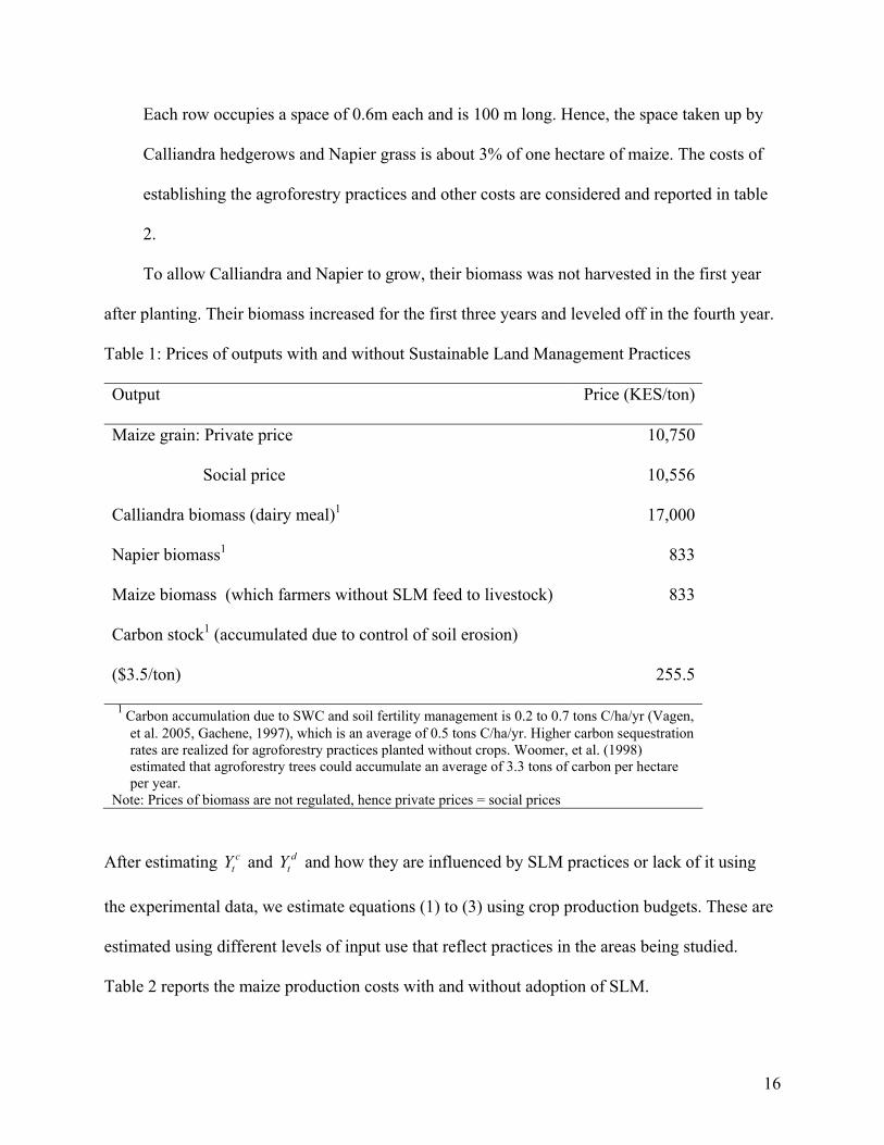
Table 1: Prices of outputs with and without Sustainable Land Management Practices

Output Price (KES/ton)

Maize grain: Private price 10,750

Social price 10,556

Calliandra biomass (dairy meal)1 17,000

Napier biomass1 833

Maize biomass (which farmers without SLM feed to livestock) 833

Carbon stock1 (accumulated due to control of soil erosion)

($3.5/ton) 255.5

1 Carbon accumulation due to SWC and soil fertility management is 0.2 to 0.7 tons C/ha/yr (Vagen, et al. 2005, Gachene, 1997), which is an average of 0.5 tons C/ha/yr. Higher carbon sequestration rates are realized for agroforestry practices planted without crops. Woomer, et al. (1998) estimated that agroforestry trees could accumulate an average of 3.3 tons of carbon per hectare per year.

Note: Prices of biomass are not regulated, hence private prices = social prices

After estimating and and how they are influenced by SLM practices or lack of it using

the experimental data, we estimate equations (1) to (3) using crop production budgets. These are

estimated using different levels of input use that reflect practices in the areas being studied.

Table 2 reports the maize production costs with and without adoption of SLM.

ctY d

tY

16

Since we are analyzing social CBA, we account for the input and output price distortions. Kenya

imports all of its inorganic fertilizer. Fertilizer is classified by the Kenya Revenue Authority as

an essential import, hence does not attract an import tax. This implies the Kenya fertilizer price is

not distorted. Kenya produces most of its maize seed locally and the government does not

regulate the maize seed price, suggesting that both inputs (fertilizer and seeds) have negligible

price distortions. However, the government participates in the maize market, contributing to

market distortions. For example the National Cereal and Produce Board (NCPB), which is a

government institution, bought 0.18 million tons of grain in the 2005/06 season, representing

about 6.7% of the maize demand in Kenya. NCPB buys maize grain at KES 13.33/kg but the

maize market price is KES 10.56/kg. However, NCPB price is paid only to 6.7% of maize

consumed in Kenya. Hence the weighted average price of maize after government intervention is

KES 10.75 (13.33*0.067+10.56*0.933) per kg suggesting that the estimated price distortion is

around KES 0.19/kg or KES 190/ton. Prices of Calliandra, crop residues, and Napier grass are

not regulated or taxed, hence have no distortions.

Kenya does not import a large volume of maize under normal circumstances. For

example, only a net of about 10,000 tons of maize was imported in 2003 (CBS, 2004) at a tariff

of 50% of CIF. Since only a small volume of maize was imported into the country, we do not

introduce the import tariff distortion in this analysis.

Estimation of off-site costs of land degradation is always difficult due to lack of data. As

discussed earlier, there are many potential local, national and global off-site effects of land

degradation. Our study will focus on the off-site effects related land management practices that

affect soil erosion and carbon stock on cropped farmland. The major off-site effects of soil

erosion include sedimentation of surface water bodies such as lakes, ponds, reservoirs and

17

18

waterways. Siltation increases the costs of water facility maintenance and replacement, and

purification and treatment of potable water, (Moore and McCarl, 1987). Soil erosion also affects

soil organic carbon and above ground vegetation. However, contribution of agriculture to

anthropogenic soil erosion is not well-known. Other anthropogenic activities such as roads could

cause significant soil erosion (Pagiola, 1999).15 Soil eroded from agricultural land also gets

deposited elsewhere within the farm or in neighboring farms while soil reaching waterways

could be deposited on the streambed. Hence the share of eroded soil reaching surface water

bodies and reservoirs is always very small. For example in large watersheds, sediment delivery

ratio, the sediment that exits the watershed as share of the gross erosion, is only 0.05 (Stocking,

1996).

In this study we estimated the costs of potable water production from Kinale/Kikuyu water

catchment is the siltation of the water reservoir at Sasumua water treatment plant, which supplies

around 20% of Nairobi city potable water. The Sasumua water treatment plant staff estimated

that the costs of water treatment and purification during the dry season reflect the costs of water

treatment and purification when all farmers effectively control soil erosion such that water

production is not affected significantly by soil erosion and other agricultural activities that

pollute water. The water treatment and purification costs with land degradation were simulated

using the rainy season. The nature of the potable water problem is siltation and pollution.

Untreated and unpurified water is characterized by higher turbidity due to solids such as soil,

crop residues, animal droppings, etc., higher bacterial count and pH, coloration and agrochemical

loading. To address these problems, water has to be treated and purified using greater amount of

alum (aluminum sulphate) - a coagulant - to purify water and chlorine to disinfect the water

(table 3).

19

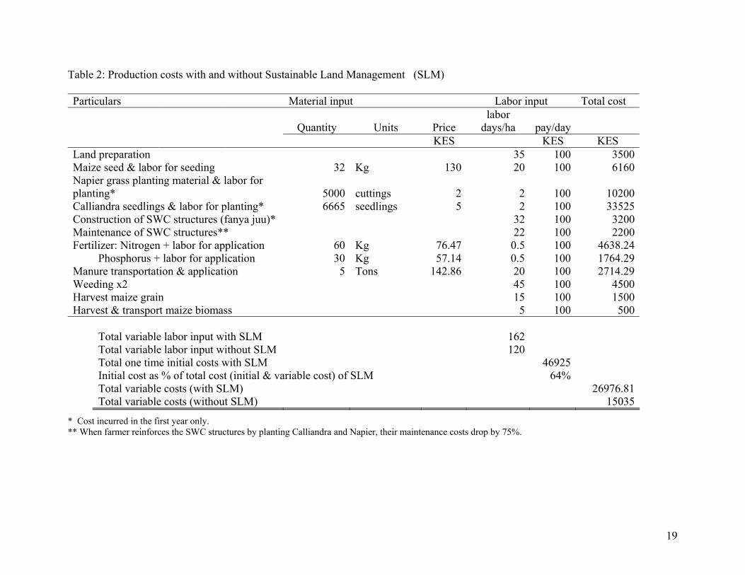
Particulars Material input Labor input Total cost

Quantity Units Price labor

days/ha pay/day KES KES KES

Land preparation 35 100 3500Maize seed & labor for seeding 32 Kg 130 20 100 6160Napier grass planting material & labor for planting* 5000 cuttings 2 2 100 10200Calliandra seedlings & labor for planting* 6665 seedlings 5 2 100 33525Construction of SWC structures (fanya juu)* 32 100 3200Maintenance of SWC structures** 22 100 2200Fertilizer: Nitrogen + labor for application 60 Kg 76.47 0.5 100 4638.24 Phosphorus + labor for application 30 Kg 57.14 0.5 100 1764.29Manure transportation & application 5 Tons 142.86 20 100 2714.29Weeding x2 45 100 4500Harvest maize grain 15 100 1500Harvest & transport maize biomass 5 100 500 Total variable labor input with SLM 162 Total variable labor input without SLM 120 Total one time initial costs with SLM 46925 Initial cost as % of total cost (initial & variable cost) of SLM 64% Total variable costs (with SLM) 26976.81 Total variable costs (without SLM) 15035

Table 2: Production costs with and without Sustainable Land Management (SLM)

* Cost incurred in the first year only. ** When farmer reinforces the SWC structures by planting Calliandra and Napier, their maintenance costs drop by 75%.

Due to elevated use of alum, there is sludge buildup that requires frequent backwashing. This process

requires use of a large amount of water that has to be disposed of after backwashing. The buildup of

silt in the water reservoirs and intakes is also cleaned by dredging. It is estimated that use of alum,

chlorine, backwashing and removal of siltation has increased water production cost by KES

9,904,041 per year.

Table 3: Increase in the cost of water treatment and purification due to land degradation

Type of treatment/purification

Treatment agent Cost without SLM (Million KES per 7 months)

With SLM (Million KES per 5 months)

Incremental cost (Million KES/year)

Purification of water Alum 8.30 1.78 5.81 Treating water Chlorine 0.39 0.16 0.17 Sludge removal Flush with water 0.53 0.11 0.43 Cleaning siltation Dredge sediments 3.50 Total incremental cost 9.91 Notes: The incremental costs are computed by multiplying additional costs of water treatment during the

wet season times the number of wet season months, rather than the difference of costs with and without SLM.

Results

Figure 1 shows that maize yield declines for both the with and without fertilizers

and crop residues. Figure 1 also shows the regression results of the crop yield model. The

rate of decline for the without fertilizer and crop residue is much faster than the case with

SLM practices, and the intercept is also lower without SLM. The predicted maize yield of

the two scenarios (figure 1) shows that in a 100 year period, maize yield with fertilizer

and crop residue in the first year was 5.5 tons/ha but will decline at a rate of 2.5%

annually, which is equivalent to about 135 kg of grain yield reduction from yield in the

previous year.. However, this rate of decline decays over time as yield decreases. The

corresponding rate of maize yield decline for the without fertilizer and crop residue

20

scenario is 3.8% per year. The crop yield trend shows the long-term impact of land

degradation resulting from continuous cultivation, which is a common problem in areas

with high population density.

Economic viability of SLM practices

An analysis was done to evaluate the economic viability of SLM practices namely

application of the recommended inorganic and organic fertilizers, incorporation of crop

residue, and use of SWC structures and stabilizing them with Calliandra hedgerow and

Napier grass. .We first consider the private and social NPV and IRR of SLM practices.

We do this by examining the NPV per hectare for all the SLM practices and the

contribution of offsite costs and benefits to NPV. There are two options that a farmer

could take to implement the initial investment. The first option involves implementing all

initial investments in the first year, namely constructing SWC structures and stabilizing

them with Calliandra and Napier grass. The second option is staggering the initial

investment over a period of time that gives the farmer the opportunity to stagger the

expensive initial investments. Investigation of the two options showed that staggering the

initial investment was more efficient than the option of investing in all technologies in the

first year.

If a farmer takes the first option by adopting all SLM practices in the first year, she will

realize a total 50 year private NPV of KES 152.31/ha. The corresponding total social

NPV is KES 176.05/ha. The initial fixed costs account for 64% of the total cost (fixed

and variable cost) of SLM practices in the first year (table 3). Almost 50% of the initial

cost is contributed by Calliandra seeds, suggesting that the legume is likely to be one of

the most important barriers to adoption if its planting material is not made cheaper and

21

more easily available. The high initial cost underscores the barrier to adoption of SLM

practices that farmers are likely to face in the initial SLM investment. This barrier may be

difficult to address for poor households.

Figure 1: Regression equation lines showing maize yield with and without SLM based on

the Kabete fertility experiment.

0.00

1.00

2.00

3.00

4.00

5.00

6.00

0 2 4 6 8 10 12 14 16 18 20 22 24 26 28 30 32 34 36 38 40 42 44 46 48

Years

tons

/ha

Maize yield w ith SLM Maize yield w ith no SLM

Y = exp(8.51+ 0.0000038rain-0.025year) P>|t| 0.000 0.960 0.007 R square 0.62

Y = exp(8.6 + 0.00004rain - 0.038year) P>|t| 0.000 0.061 0.016 R square 0.59

With SLM

With no SLM

Table 4: Fifty year social and private NPV, IRR and off-site benefits and costs

Private Social Total NPV (‘000 KES/ha) 152.31 176.05 Average NPV/year (‘000 KES/ha) 3.05 3.53 Value of carbon sequestered as % of NPV 10.00 Cost of water treatment and purification as % of NPV 4.79 IRR (%) 30.70 39.00 Notes: (i) The total water treatment costs were divided by the total area cultivated in the catchment

(ii) Carbon sequestered include carbon saved in the crop plot due to control of soil erosion (0.5 tons/ha/year) and Calliandra and Napier underground and above ground carbon

22

Staggering investment lowered significantly the losses incurred if a farmer follows a one

time investment plan from around KES 50,000/ha for the private NPV to total of only

KES 15,430/ha if initial investments are staggered over a period of four years. The IRR

rates obtained in this study (39% for the social NPV and 30.7% the private NPV), are

comparable to those obtained in other SWC studies conducted in Central America and the

Caribbean, where SWC IRR ranged from 11% to 84% (Lutz, et al., 1994). The social

NPV and IRR results suggest that holding all else constant, adoption of SLM practices is

profitable. The private NPV and IRR also show that this is true even when we ignore the

offsite costs and benefits.

The social NPV is higher than the private NPV due to valuation of the carbon

stock resulting from biomass production of Calliandra and Napier grass and due to

imputing costs of the off-site negative impact of soil erosion for the without SLM

scenario (table 4). The global benefits resulting from carbon sequestration account for

about 10% of the total NPV/ha and the costs due to water treatment and purification was

about 5% of the social NPV. The contribution of offsite costs and benefits is significant

and indicates the large costs that farmers may have to pay to account for costs that they

do not have direct benefits. Farmers and other land users always receive no compensation

for the environmental services they provide to the public. This contributes to their

common attitude of disregarding the externalities of their production and sub-optimal

land use. In The case of Kenya, Payment for Environmental Services (PES) is still limited

to services related to game parks. Most environmental services offered by farmers do not

receive compensation.

23

To understand the robustness of the results, we need to analyze the sensitivity of

the NPV and IRR to changes in the input and output prices.

Sensitivity analysis

We analyze the sensitivity of the NPV and IRR to input and output prices and to

presence or absence of a dairy sector. We halve the maize price and double the fertilizer

price and analyze the response of NPV and IRR to such changes. In table 5, we take a

pessimistic scenario whereby the price of maize falls by 50% from KES 10,750 to KES

5,375 per ton. This leads to a 25% drop in the social 50 year total NPV from KES

176,050 to 131,990 per hectare for farmers with SLM practices (table 5). The private

NPV drops by 28% while the private and social IRRs drop only slightly. The drop of

NPV for the farmers who practice SLM is cushioned by the revenue from Calliandra and

Napier biomass, suggesting that adoption of agroforestry practices involving multi-

purpose trees and shrubs reduces risk exposure.

If the fertilizer prices double, the social and private NPV decreases to levels

comparable to those experienced after the 50% fall in maize price. If fertilizer prices

double and maize price falls by 50%, the total 50 year social NPV for adopting SLM

practices will fall by about 50% but the corresponding IRR for adopting SLM practices

will be greater than the discount rate of 10% (table 5). These results suggest that adoption

of SLM practices is profitable over a wide range of output and input prices.

We investigated the feasibility of adopting the SLM practices in an area with no

economic use for the Calliandra and Napier biomass. Such areas could have weak or no

dairy production activities. Table 5 shows that if Calliandra and Napier grass biomass are

not used for dairy production, the total 50 year social and private NPV drop dramatically

24

to KES 39,190 and KES 7,790 per hectare respectively. The corresponding IRR is 10%

for the social scenario and about 1.9% for the private scenario (table 5). These results

demonstrate that profitability of the SLM practices heavily depends on the dairy sector or

other synergistic benefits of the SLM practices. Without dairy production, the NPV and

IRR for adopting SLM practices are also very sensitive to changes in input and output

prices. A 50% decrease in maize price leads to negative 50 year total NPV for both

private and social scenarios. In general changes of all input prices leads to negative social

and private NPV. The results suggest that in areas with weak or no dairy production or

other enterprises that have synergies with some practices, SLM practices have low

returns and are risky and hence not likely to be adopted. Hence in the absence of PES or

other incentives, farmers in areas with weak or no dairy production are not likely to adopt

the SLM practices analyzed in this research and consequently prevent the negative offsite

effects of land degradation. This is a major concern that needs to be addressed while

promoting adoption of the SLM practices in areas with weak or no dairy production.

Table 5: Sensitivity analysis of NPV and IRR with no dairy sector, double fertilizer prices

Change Social NPV (KES ‘000)

Private NPV (KES ‘000)

Social IRR (%)

Private IRR (%)

Baseline (no change) 176.05 152.31 39.00 30.70Half maize price 131.99 109.03 42.0 29.5

Half maize price and double fertilizer price

90.29 67.33 25.0 15.8

Fertilizer prices rise by 50% 134.55 110.61 27.0 19.7

No dairy 39.19 7.79 10.0 1.9

No dairy, half maize price -4.86 -35.49 - -

No dairy, double fertilizer price -2.51 -33.91 - -

No dairy, double fertilizer price, & half maize price

-46.52 -77.19 - -

25

Conclusions and implications

This study investigated the private and social returns to the Sustainable Land

Management (SLM) practices with an objective of finding practices that will reduce the

on-farm and off-farm negative effects land degradation. The Net Present Value (NPV) of

the SLM practices was much greater than zero indicating SLM practices are profitable

when they are complementary. In particular, use of Soil and Water Conservation (SWC)

structures and reinforcing them with agroforestry practices are profitable when the

agroforestry practices (Calliandra and Napier) are used as fodder for dairy cows. These

results suggest that SLM practices have the potential to be adopted in areas with a strong

dairy production. This will address both the on-farm and off-farm negative impacts of

land degradation.

One of the major concerns for widespread adoption of SLM practices is the high

initial investment cost required to establish SWC structures and reinforce them with

multipurpose agroforestry shrubs and grass. This concern comes from the fact that most

farmers have limited capacity to invest and consequently high private discount rates. The

initial costs account for 64% of the total cost of maize production in the first year. If a

farmer decides in the first year to adopt all the SLM practices, she will incur a loss of

about Kenyan Shillings (KES) 50,000/ha in the first year, which is about a third of the

household income in Kenya. The initial investment cost is certainly a barrier to adopting

SWC structures and agroforestry and this explains their low adoption. One strategy that

farmers are likely to use to address this constraint is to stagger the initial investments

over several years. Even after staggering the initial investment costs over a period of

three to four years, the farmer will still incur initial losses of about KES 15,430/ha over

26

the four year investment period, implying that some farmers may not be able to adopt

SLM practices even if they have the option to stagger the initial investment.

These results have important implications for addressing the off-site impacts of

land degradation. There is need to facilitate availability of credit in the operational areas

to help farmers’ finance these initial investment costs. However, credit in the form of

cash may not work due to the fungible nature of cash. In kind credit, such as providing

agroforestry planting materials could help farmers to obtain them easily. Establishment of

commercial agroforestry nurseries will greatly help the largest initial cost of buying

Calliandra and Napier or any other agroforestry tree/shrubs/grasses in the first year.

To reflect the biophysical and socio-economic diversity in the study area, we

investigated the profitability of SLM practices in areas that have a weak or no dairy

production sector. The results show that in areas with weak or no dairy production, the

SLM practices to be promoted by this project are risky when agricultural prices change

significantly. These results suggest the need to promote SLM practices that complement

each other and other farm enterprises. This also implies that promoting a package of

complementary technologies is likely to make them more profitable and less risky. As

discussed above however, a package of technologies implies high initial fixed costs or

variable costs, and hence the need to promote financing services. In the quest to promote

a package of technologies, stepwise adoption (Byerlee, et al., 1986) of components of the

technologies should be expected. For example, SWC structures need to be planned such

that they involve agroforestry practices that have alternative uses such as dairy, firewood,

etc. Our study has shown that promotion of agroforestry practices for the sake of control

of soil erosion and its off-site effects only may not work.

27

If promotion of a mix of complementary enterprises is not feasible, high value

crops are likely to make SLM practices more profitable (Place, et al., 2002). However,

risk and access to market are likely to be of concern for high value crops.

In areas where SLM practices are not profitable, promotion of alternative livelihoods is

necessary. For example, non-farm activities are likely to give farmers alternatives to their

land degrading agricultural activities. For example, a study in Uganda showed that

farmers who had non-farm activities were more likely to fallow than those without

(Nkonya, et al., 2005).

Another approach that could increase the feasibility of adoption of SLM practices

is Payment for Environmental Services (PES). For PES to be sustainable it needs to be

win-win, i.e. it increases returns to SLM practices and also helps downstream

communities to avoid or minimize the off-site effects of land degradation. For example, if

the Sasumua Water Treatment Plant were to pay farmers to adopt soil and water

conservation technologies, it could reduce its potable water production costs and help

farmers to realize profit by adopting SLM practices. The project will need to explore the

possibility of PES since such environmental service payments are not necessarily feasible

or economic wherever there are off-site costs, considering the costs of establishing and

monitoring such a payment system.

28

Endnotes:

1 The Sasumua dam, located on Chania river, receives water from a catchment of around

128 km2 (Annandale, 2002).

2 As it will be shown later, the price distortions relevant for this study are negligible.

3 Other studies report higher private discount rates (for example Holden, et al., 1998 for

evidence from Ethiopia, and Pender, 1996 for evidence from south India).

4 Alternative valuation techniques include the ‘hedonic pricing approach’ and the

‘replacement costs approach’. However, the ‘change of productivity approach’ is the

most commonly applied and widely accepted tool (for more details on the various tools

see Enters, 1998).

5 More details of these experiments are given in the data section below.

6 In addition to depleting SOM, continuous cultivation even with adequate N, P, and K

inorganic fertilizers could lead to depletion of nutrients other than N, P, and K, and

degradation of biological physical properties of the soil.

7 Except rainfall that is controlled for in equation (5), and (6).

8 More details in the data section.

9 Since Embu is located in the high potential area as most of the watersheds, these soil

erosion trial data reflect better the biophysical environment of the selected watersheds

than the Machakos soil erosion experimental results that were used by Pagiola (1996).

Machakos is located in much drier areas with different soil characteristics.

10 The Kenya Agriculture Act (Cap 318) of 1980 prohibits agricultural activities on land

with slope exceeding 35%. The law also requires that farmers must have SWC structures

on crop plots with slope of 12% to 35% (Government of Kenya, 1986).

29

11 The experiment at Kabete is established on plots with very small slope that does not

require any form of SWC structure. Hence it reflects the yield of crops planted on steep

slopes but with SWC structures that effectively control soil erosion.

12 Results from a similar experiment conducted at Machakos Kenya showed that one cm

loss of soil topsoil depth led to a loss of 0.13 tons of maize grain yield/ha (Pagiola, 1996),

which was equivalent to about 7% of the yield with zero soil loss. The rate of loss of crop

yield due to erosion is less in more fertile soils such as volcanic soils (andosols and

nitisols) that are rich in nutrients (Mantel and van Engelen, 2000).

13 Agroforestry practices also increase soil nutrient inputs; enhances internal flows;

decrease nutrient losses and other provide environmental benefits (Sanchez, et al., 1997)

14 Maize yield in the Kabete long-term soil fertility trial also showed poor response to

fertilizers in the first few years, probably due to the same reason (high SOM on plots

after opening a virgin land). The agroforestry trees and shrubs are likely to show stronger

impact on yield of crops grown on land with low SOM and soil nutrients (Sanchez, et al.,

1997; Woomer, et al., 1998). Hence it was expected that maize yield in the Embu

agroforestry trial will show a greater response to the agroforestry treatment in the

subsequent years.

15 Ecological erosion can also contribute significantly to soil erosion. It is estimated that

ecological erosion of undisturbed forest area is about 20 – 30 t/km2/year (Shepherd, et al.,

2000).

30

References

Annandale, G. 2002. Assessment of Reservoir and Intake Sedimentation at Selected Sites

in Kenya. Consultancy Report by Engineering and hydrosystems Inc. submitted to

the World Bank, Washington D.C.

Batjes, N.H. 2004. “Soil carbon stocks and projected changes according to land use and

management: a case study for Kenya,” Soil Use and Management, 20(3):350-356.

Byerlee, D. and H.E. de Polanco. 1986. “Farmers Adoption Stepwise Adoption of

Technological Packages: Evidence from the Mexican Altiplano.” American

Journal of Agricultural Economics, 68:519-527.

Dixit, A.K. and R.S. Pindyck. 1994. Investment under Uncertainty. Princeton, N.J.:

Princeton University Press.

Duxbury, I. 1995. “The significance of Greenhouse Gas Emission from Soils of Tropical

Agroecosystems.” In Lal, R., J. Kimble, E. Levine, and B. Stewart, (eds). Advances in

Soil Science, Boca Raton:CRC Press.

Enters, T., 1997. Methods for the Economic Assessment of the On- and Off-Site Impacts

of Soil Erosion. International Board for Soil Research and Management. Issues in

Sustainable Land Management No. 2. Bangkok: IBSRAM.

Fafchamps, M. and J. Pender. 1997. Precautionary Saving, Credit Constraints, and

Irreversible Investment: Theory and Evidence from Semiarid India. Journal of

Business and Economic Statistics 15(2): 180-194.

31

Government of Kenya. 1986. Laws of Kenya: The Agriculture Act. Government Printer,

Nairobi Kenya.

Holden, S., B. Shiferaw., M. Wik. 1998. Poverty, Credit Constraints and Time Preference

of Relevance for Environmental Policy Environment and Development Economics,

3:105-130.

ICRAF (International Center for Research in Agroforestry). 2005. Trees of Change: A

Vision for an Agroforestry Transformation in the Developing World. World

Agroforestry Center, Nairobi Kenya.

Koning, N., E. Smaling. 2005. Environmental Crisis or ‘Lie of the Land’? The Debate on

Soil Degradation in Africa. Land Use Policy 221):3-11.

King, G. 1993. “Conceptual Approaches for Incorporating Climatic Change into the

Development of Forest Management options for Sequestering Carbon.” Climate

research 3:61-78.

Lutz, E., Pagiola, S., and C. Reiche. 1994. Economic and Institutional Analyses of Soil

Conservation Projects in Central America and the Caribbean. World Bank

Environment Paper Number 8. Washington D.C.: The World Bank.

Mantel, S., V. Van Engelen. 2000. “Assessment of the Impact of Water Erosion on

Productivity of Maize in Kenya: an Integrated Modeling Approach,” Land

Degradation & Development 10(6):577 – 592.

Moore, W., and B. McCarl. 1987. “Off-site Costs of Soil Erosion: A Case Study in

Willamette Valley.” Western Journal of Agricultural Economics, 12(1):42-49.

32

Nandwa, S.M. and M.A. Bekunda. 1998. “Research on Nutrient Flows and Balances in

East and Southern Africa: State of the art,” Agriculture, ecosystems and Environment

71:5-18.

Nkonya, E.M. 1999. Modeling Soil Erosion, Fertility Mining, and Food Import Quality

Enforcement: The Case of Wheat in Northern Tanzania. A Dssertation Submitted in

Partial Fulfillment of the Requirements for the Degree Doctor of Philosophy,

Department of Agricultural Economics, College of Agriculture, Kansas State

University, Manhattan, Kansas.

Nkonya, E.M., J. Pender, C. Kaizzi, K. Edward, and S. Mugarura. 2005. Policy Options

for Increasing Crop Productivity and Reducing Soil Nutrient Depletion and Poverty

in Uganda. Environment and Production Technology Division (EPTD) Discussion

Paper # 134. International Food Policy Research Institute (IFPRI), Washington D.C.

Oldeman, L.R.; R.T. Hakkeling, W. Sombroek. 1991. World Map of the Status of

Human-induced Soil Degradation. International Soil Reference and Information

Center. Wageningen and United Nations Environmental Program, Nairobi Kenya.

Oldeman, R. 1994. “The Extent of Global Soil Degradation” In: Greenland D., and I

Szabolics (eds). Soil Resilience and Sustainable Land Use, CAB International,

U.K.

Pieri, J.M. 1989. Fertility of soils. A Future for Farming in the West African Savannah.

Springer-Verlag, New York.

33

Pagiola, S., 1999. Global Environmental Benefits of Land Degradation Control on

Agricultural Land. World Bank Environment Paper No. 16. Washington D.C.: The

World Bank.

Pagiola, S., 1996. Price Policy and Returns to Soil Conservation in Semi-Arid Kenya. In:

Environmental and Resource Economics 8: 255-271.

Pender, J. 1996. “Discount Rates and Credit Markets: Theory and Evidence from Rural

India.” Journal of Development Economics, 50, 257-296.

Place, F. and P. Hazell. 1993. “Productivity effects of indigenous land tenure systems in

sub-Saharan Africa.” American Journal of Agricultural Economics 75(1): 10-19.

Place, F., Swallow, B.M., Wangila, J.W., Barrett, C.B. 2002. “Lessons for Natural

Resource Management Technology Adoption and Research,” in Barrett, C.B.,

Place, F., Abdillahi, A., (eds), 2002b. Natural Resources Management in African

Agriculture: Understanding and Improving Current Practices, CABI,

Wallingford, UK.

Renard, K.G., G.R. Foster, G.A. Weesies, and J.P. Porter. 1991.” RUSLE: Revised

Universal Soil Loss Equation.” Journal of Soil and Water Conservation 46(1):

30-33.Scherr, S. and S. Yadav. 1996. Land Degradation in the Developing World:

Implications for Food, Agriculture and the Environment to 2020. Food,

Agriculture and Environment Discussion Paper #14., International Food Policy

Research Institute, Washington D.C.

Sanchez, P.A, R.J. Buresh, R. R. Leakey. 1997. “Trees, Soils, and Food Security.”

Philosophical Transactions of the Royal Society of London, Series B, 352:949-961

34

Scherr, S. 2000. “A Downward Spiral? Research Evidence on the Relationship between

Poverty and Natural Resource Degradation.” Food Policy, 25:479-498.

Scherr, S. and S. Yadav. 1996. Land Degradation in the Developing World: Implications

for Food, Agriculture and the Environment to 2020. Food, Agriculture and

Environment Discussion Paper #14., International Food Policy Research Institute,

Washington D.C.

Shepherd, K., M. Walsh, F. Mugo, C. Ong, T. Svan Hansen, B. Swallow, A. Awiti, M.

Hai, D. Nyantika, D.Ombalo, M. Grunder, F. Mbote and D. Mungai. 2000.

Improved land management in lake Victoria basin: Linking Land and Lake,

Research and Extension, Catchment and Lake Basin. International Centre for

Research in Agroforestry and Kenya Ministry of Agriculture and Rural

Development, Soil and Water Conservation Branch, National Soil and Water

Conservation Programme. Working Paper 2000-2 International Centre for

Research in Agroforestry (ICRAF).

Schroeder, P. 1993. “Agroforestry Systems: Integrated Land Use to Store and Conserve

Carbon.” Climate Research 3:53-60.

Stocking, M. 1996. “Soil Erosion: Breaking New Ground.” In: M. Leach and R.

Mearns (eds.), The Lie of the Land: Challenging Received Wisdom on the African

Environment. London: The International African Institute in association with

James Currey, pp 140-154.

Unruh, J.D., R.A. Houghton and P.A. Lefebvre. 1993. “Carbon Storage in Agroforestry:

an Estimate for Sub-Saharan Africa”, Climate Research 3:39-52.

35

Vagen, T.-G., Lal, R. and B.R. Singh, 2005. “Soil Carbon Sequestration in Sub-Saharan

Africa: A Review.” In: Land Degradation and Development 16, 53-71.

Voortman, R., B. Sonneveld and M. A. Keyzer. 2000. African Land Ecology:

Opportunities and Constraints for Agricultural Development. CID Working

Papers no 37. Harvard University: Center for International Development.

Weibe, K. 2003. Linking Land Quality, Agricultural Productivity and Food Security.

Agricultural Economic Report No. 823, Economic Research Service, U.S.

Department of Agriculture.

Woomer, P.L., C. Palm, J.Qureshi, J. Kotto-Same. 1998. “Carbon Sequestration and

Organic Resource Management in African Smallholder Agriculture.” In: Lal, R.,

J. Kimble, R. Follett, and B. Stewart (eds). Management of Carbon Sequestration

in Soil. Advances Soil Science. CRC Press: 153-173.

World Bank. 2005. Word Development Indicators 2005. World Bank, Washington DC.

36