1

Our first lecture will address basic quantities and units in radiological physics.

2

The objectives of this lecture will be to enable you to become familiar with the basic units of radiological physics.

At the conclusion of this lecture, you should be able to differentiate between a physical quantity and its unit of measurement; we will classify quantities as basic quantities, supplementary quantities, derived quantities, and special quantities.

In addition, I want you to become comfortable in converting units of measurement.

Next we will review how we write numbers in scientific notation. I think that should be a review for all of you as you have likely seen scientific notation in your various college science courses.

3

Then we will identify the various prefixes used in SI, the international system of units.

We will then differentiate between stochastic and deterministic quantities. Certain quantities we encounter in Radiation Physics are stochastic and others are deterministic. We want to know which is which, what the difference is between the two, and how they are related.

We will then talk about accuracy and precision in measurement. Most of what we do in radiological physics involves measurement so we need to be able to differentiate between accuracy and precision.

And finally, we want to know what the sources of error in doing measurements are and we want to be able to estimate our error.

4

We will begin our lecture with a discussion of physical quantities and units.

We define a physical quantity as something that characterizes a physical phenomenon, something that we can measure, in terms that are amenable to numerical specification.

I want to appeal to a gut understanding of what a physical quantity is: some of these physical quantities are length, mass, velocity, etc. Every physical quantity can be written it in terms of two entities, the numerical value for the physical quantity and the unit associated with the physical quantity. The unit is just a selected reference sample of that quantity.

I am going to give you a word of advice when you are doing problems in medical physics: keep track of units. Very often if you don’t quite know how to solve a problem, by trying to sort out units you may get some insight into how to solve the problem. It is one of the strategies we can use.

Also keeping track of units will keep you from making horrendous mistakes. Like for example, expressing energy in ergs rather than in joules. The difference between the two is a factor of about 107. You don’t want to make errors of the magnitude of 107. Those kinds of errors are disastrous.

Nor do you want to make errors of 101 or 102. Those could also be disastrous too.

By keeping track of units you may be able to avoid or mitigate the risk of those kinds of errors.

If I see on any problem set that you’ve left off units, you are going to be dinged pretty badly for that. Keep in mind that keeping track of units is very important.

5

It is also important to differentiate between a physical quantity and a unit of measurement.

Here is an example: The mass of a rock is 83 kg. In this case, the physical quantity is the mass, the numerical value of the physical quantity is 83, and the units are kilograms.

6

We are not allowed to define a physical quantity as a certain number of units of that physical quantity.

Why do I make this distinction? I am making this distinction partially for historical reasons. There was a time when a quantity called “radiation exposure” was defined to be the number of Roentgens. Well that is completely wrong. We cannot define something in terms of its units. Physicists very shortly after they did this realized the mistake they made and developed a new definition of exposure in term of physical quantities. We’ll talk about that a bit later. It gets a bit tricky when we are trying to define some radiation quantities.

We do not define a quantity in term of its units.

We are not allowed to say “Mass is the number of kilograms.”

We are not allowed to say “Distance is the number of meters.”

Mass and distance are quantities; kilograms and meters are the units that we use to measure the quantities.

7

We also have systems of units.

There is an organization called the International Commission on Weights and Measures, abbreviated CIPM. Note that in French, everything is reversed. They have adopted what is called the International System of Units, abbreviated SI. Most of the quantities that we deal with in radiological physics are expressed in terms of SI units. There will be a few exceptions, and I will identify those exceptions when we encounter them, but most of the quantities will be expressed in SI units.

If you want to publish a paper in any of the standard radiological journals, or radiological physics journals, you have to use SI units -- it is the rule of the journal.

There are special units that we use in radiation, and there is an organization called the International Commission on Radiation Units and Measurements, abbreviated ICRU. (Fortunately this uses the English language; otherwise it would be called CIUR). The ICRU, and you will be hearing about the ICRU all throughout your careers, has advised the adoption of some special units for radiation.

So what are these quantities; what are the basic quantities, what are the derived quantities and what are the special quantities.

8

Basic quantities are defined really arbitrarily: they include length, mass, and time as basic quantities. In effect, we say these are almost like mathematical axioms.

In mathematics we say: Here are a couple of statements we assume to be true.

Similarly, here we will say: Here are a couple of units that we don’t really define; we kind of have an intuitive feel for what length is, the distance between two points. Well then, what’s distance, the length of a line between two points. You can see wedevelop some circular reasoning.

Basic quantities also include mass and time.

It is interesting that one of the basic quantities is electric current. I have no idea why electric current is basic. I would think the charge is more basic than electric current. I am not going to argue with the folks that generate the SI units.

Temperature is another basic unit. Amount of a substance is a basic unit. Luminous intensity is also a basic unit. If you are doing Imaging Physics you might have to worry about luminous intensity. And maybe if you are doing some work with lasers, you will have to deal with luminous intensity.

9

So now that we now have the basic quantities we need to know the units for the basic quantities. In fact, we need to know the SI units.

The actual units themselves are maintained by standards laboratories, and everything that we measure is compared against a standard. It used to be that the unit of length was measured by two scratches in a metallic bar inside of a vault kept just outside of Paris. Now we are a little more sophisticated and we need to be much more precise, so we define our units in terms of a certain wavelength of light.

Whatever they are, there are standards and we compare everything to the standards.

The standard unit of length is the meter. The standard unit of mass is the kilogram; why it is not the gram, I am not sure, but it is the kilogram. The unit of time is the second. The unit of electric current is the Ampere. The unit of temperature is the Kelvin. The unit of the amount of a substance is the mole and the unit of luminous intensity is the candela.

10

There are some supplementary quantities. Some of these are dimensionless having to do with angles, such as the plane angle. The unit of plain angle is the radian. We are also going to talk a lot about solid angles and the unit of measurement of solid angle is the steradian.

There are 4π steradian in a sphere; 2π radian in a circle.

Those are some of the supplementary quantities. We are especially interested in the angles. We are going to be talking about scatter of radiation. We are going to be concerned about where the radiation is going off. How much is going off in what direction. We will see that a little bit later on in the course.

11

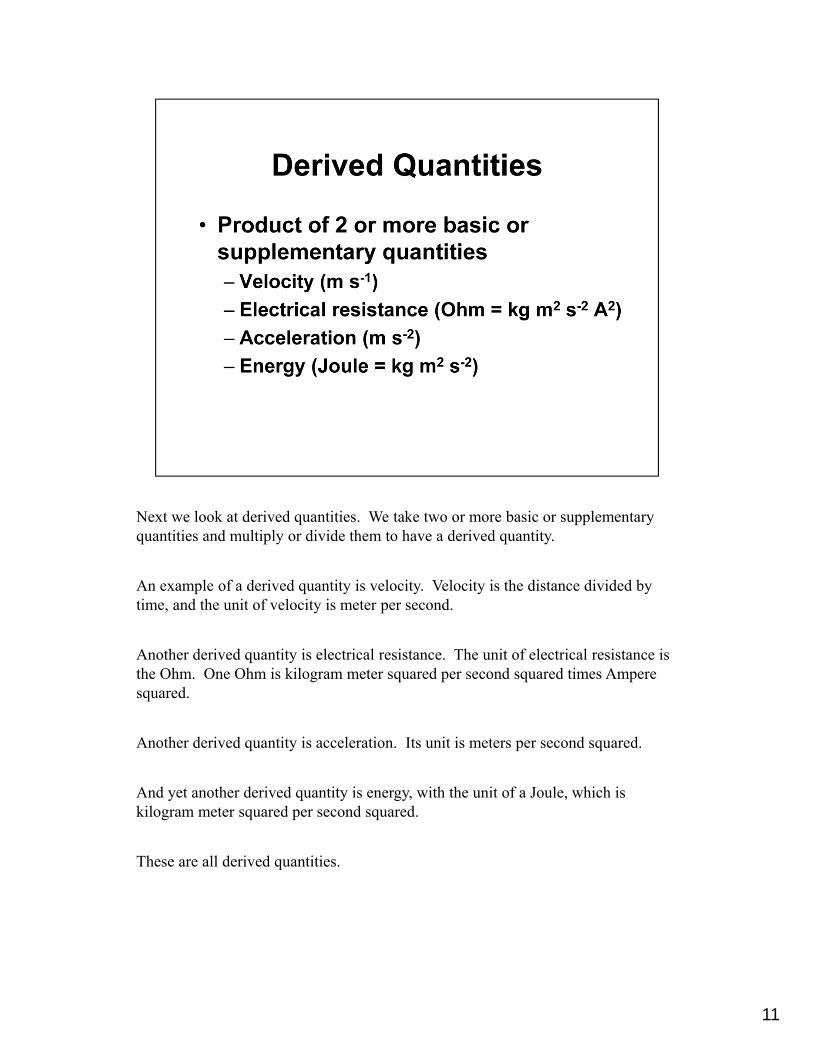
Next we look at derived quantities. We take two or more basic or supplementary quantities and multiply or divide them to have a derived quantity.

An example of a derived quantity is velocity. Velocity is the distance divided by time, and the unit of velocity is meter per second.

Another derived quantity is electrical resistance. The unit of electrical resistance is the Ohm. One Ohm is kilogram meter squared per second squared times Ampere squared.

Another derived quantity is acceleration. Its unit is meters per second squared.

And yet another derived quantity is energy, with the unit of a Joule, which is kilogram meter squared per second squared.

These are all derived quantities.

12

Finally, there are special quantities. These are quantities that are specific to a field of physics. They are recognized by the official authorities, which for us is the ICRU (International Commission on Radiation Units).

Here is an example: The SI unit of radioactivity is the Becquerel. It is equal to one disintegration per second. One reciprocal second – one per second.

But that is specific to radioactivity.

Another example of a specific unit is the Hertz. One Hertz is one per second.

One per second is a Hertz. One per second is a Becquerel. How many Becquerel are there in a Hertz? The answer is undefined. The Becquerel and the Hertz are specific to two different areas of physics. The Becquerel is specific to radioactive decay, while the Hertz is specific to electrical frequencies. We can’t measure electrical frequency in Becquerel even though we can measure frequency in reciprocal seconds.

So we use the Hertz for frequency and we use the Becquerel for radioactivity. Even though they have the same units, we have to use them in their specific applications.

13

Let’s now talk about keeping track of units. Many physical problems can be simplified and errors prevented by keeping track of units.

You need to keep track of units explicitly.

You are going to have a couple of problems on your problem sets where you need to convert from one set of units to another.

Here’s an example: A radioactive source emits radiation at a dose rate of one rad, (whatever a rad is—it’s an old unit of radiation dose) per hour per square meter. What is this dose rate in Gray per second per square centimeter? This is an example of the kind of calculation you should be able to do with your eyes closed.

14

We start with one rad per hour per meter squared.

First of all we must convert rad to Gray, 10-2 Gray per rad. One rad is the same as a centigray. Rad is the old unit, Gray is the new unit.

You have to multiply by 10-2 Gray per rad in the numerator. In the denominator we multiply 60 minutes per hour to get rid of the hours, 60 seconds per minute to get rid of the minutes, 100 centimeters per meter quantity squared to get rid of the meter squared. So it’s10-2 Gray divided by 3600, 60 x 60, times 104 seconds square centimeters. So this radioactive source dose rate is 2.8 x 10-10 Gy per second per centimeter squared. That’s how we do this kind of problem.

This conversion of units should be fairly straightforward.

15

We will be using a lot of large and small numbers in this course, and we have scientific notation to reduce the numbers to manageable sizes.

In expressing a number in scientific notation, we place the decimal point immediately before or immediately after the first significant figure. As an example, the number 4,321 can be expressed either as 4.321 x 103 or as 0.4321 x 104. The number 0.001234 can be expressed either as 1.234 x 10-3 or as 0.1234 x 10-2.

Use scientific notation, in general, for most of your problems, as it will be easier to handle than a lot of zeros.

In order to express quantities in scientific notation, we need to introduce the concept of significant figures. Significant figures are defined to be those digits that carry meaning contributing to the precision of a quantity. Generally, all digits carry meaning with the following exceptions:

Leading and trailing zeroes that serve as placeholders to indicate the scale of a number are not significant figures.

Spurious digits that are introduced, for example, by calculations carried out to greater accuracy than that of the original data, or measurements reported to a greater precision than the equipment supports are not significant figures.

An example of the latter is expressing a patient dose as 6325.4 cGy. That extra 0.4 cGy implies a precision greater than what is warranted and is really misleading. Generally radiation doses are expressed to the nearest cGy; I would even venture to say that expressing the dose as 6320 cGy is even more indicative of the actual precision.

16

How do we determine which figures are significant? We use the following rules:

1. All non-zero digits are considered significant. So in the number 123.45, all digits are significant.

2. Zeros appearing anywhere between two non-zero digits are significant. In the number 101.12, the 0 is a significant digit.

3. Leading zeros are not significant. In the number 0.00012, none of the zeros are considered significant figures.

17

4. Trailing zeros are always significant figures. Consequently it is important to note that when you write a number and include trailing zeros, you are saying something about the precision of a number. There is a difference between 12.23 and 12.2300.

18

Finally, there is some ambiguity in trailing zeros in a number not containing a decimal point. For example, it is not clear whether the number 1300 is accurate to the nearest unit, in which case the two zeros would be significant, or it is accurate to the nearest hundred, in which case the two zeros are not significant figures. If the former is indeed the case, the ambiguity could be removed by writing the number as 1300. Note that this number is different from 1300.0, in which the zero after the decimal point is a significant figure.

19

20

Let’s move on to the SI prefixes, which are shorthand for powers of tens.

SI rules say you have to have prefixes for 10 to the plus or minus 1, plus or minus 2, plus or minus 3, and then in increments of 3, that is, plus or minus 6, plus or minus 9, plus or minus 12. Here are a whole bunch of them; I think you are probably familiar with these.

21

We can even go further; we can go down all the way to 10-24 and 10+24. I don’t know if you have even heard of some of these. Anyway, you now have them and you can refer to them at anytime.

You can really impress your friends.

A very important concept in radiation physics is the difference between stochastic and deterministic quantities

22

23

A stochastic quantity has a value that occurs randomly. There is no way that we can predict the explicit value of a stochastic quantity. Its values are probabilistic and the probability is determined by a distribution. Stochastic values are defined for finite as opposed to infinitesimal domains only. The value of a stochastic quantity varies discontinuously with space and time.

I’ll give you some examples of stochastic quantities in a few minutes.

It is meaningless to speak of the rate of change of a stochastic quantity because a stochastic quantity represents an isolated event. The expectation value, however, of a stochastic quantity is the mean value of the measured values as the number of observations approaches infinity. The expectation value of a stochastic quantity is a deterministic one.

24

A deterministic quantity is represented as a point function. It’s continuous, and it’s a differentiable quantity of time and space. We can talk about gradients of a deterministic quantity; we can talk about the rate of change of a deterministic quantity. A deterministic quantity can be predicted by calculation and it can be estimated as the average value of observed values of associated stochastic quantity.

25

Here’s a connection: A quantity that is subjected to statistical fluctuations is stochastic but the mean value of this quantity is deterministic.

So far, the differentiation between stochastic and deterministic has been sort of abstract. Let me give you some examples that ought to illustrate this difference more clearly.

Let’s look at a coin flip. If I flip a coin, can anybody tell me with absolute certainty whether I will get heads or tails?

Of course not. Flipping a coin is a stochastic process; we can’t predict the outcome of an individual coin flip. On the other hand I may ask that if I flip a coin a hundred times what is the most likely value for number of heads. It’s going to be fifty unless I have a loaded coin. The expectation value of heads is 0.5. The expectation value of tails is 0.5. So the expectation value is deterministic. The individual coin flip is stochastic.

26

Here’s another example. I have a radioactive cobalt source. Now I want to look at a specific cobalt nucleus. I know that it’s going to decay. Do I know when it’s going to decay?

Absolutely not.

I have no idea of when a specific nucleus is going to decay. But I do know, however, that in one month, 1.5% of the nuclei will undergo radioactive decay. The stochastic process is the decay of an individual cobalt nucleus. The deterministic process is the 1.5% per month activity. We will learn about activity in our next lectures.

27

28

Here is yet another example:

We are looking at an individual event in which a photon deposits energy into an atom. The energy imparted in a specific interaction, that is the energy per unit mass, is called the specific energy. The specific energy is a stochastic quantity because we have no idea whether or not an interaction will take place, or if it does, how much energy will be deposited in the target. The interaction is a single isolated event. However the mean energy deposited per unit mass, which is the absorbed dose, is a deterministic quantity. We can do calculations involving the absorbed dose.

We can’t do very much with the specific energy because we never really know when the specific interaction occurs.

Isolated events are stochastic quantities; mean expectation values of these events, when you have a large number of them, are deterministic quantities. We will primarily be working with deterministic quantities in this course, but at times we will look at stochastic quantities.

When you are measuring radiation dose you are looking at the transfer of energy from the incident radiation to target atoms and molecules. The events in which the transfer occurs are individual stochastic events. The distribution of measured values of these independent stochastic events follows what’s called a Poisson distribution. When we have a large number of such events, we can approximate the Poisson distribution by a Gaussian distribution.

The equation shown here is the equation for a Gaussian distribution. The factor of one over root 2 π is simply there to normalize the distribution, to make the integral of the probability from minus infinity to plus infinity equal to one. The key component of the Gaussian distribution is this exponential. The quantity x is the measured value, is the mean value, and is a measure of the spread of the distribution.

A small value of means a highly peaked distribution; a large value of means a fairly broad distribution.

So with the Gaussian distribution we will see a lot of things and we will follow a lot of quantities.

29

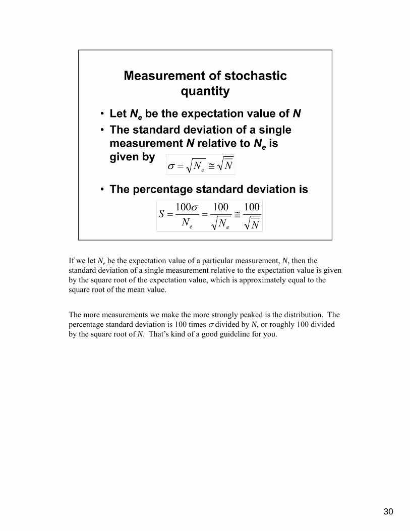
If we let Ne be the expectation value of a particular measurement, N, then the standard deviation of a single measurement relative to the expectation value is given by the square root of the expectation value, which is approximately equal to the square root of the mean value.

The more measurements we make the more strongly peaked is the distribution. The percentage standard deviation is 100 times divided by N, or roughly 100 divided by the square root of N. That’s kind of a good guideline for you.

30

What do we mean by , the standard deviation of a Gaussian distribution?

If the measured values of the stochastic quantities behave according to a Gaussian distribution, a single measurement will have a 68.3% chance of lying within plus or minus 1 of the expectation value, a 95.5% chance of lying within 2 , and a 99.7% chance of lying within 3 of the expectation value.

If we know what is for a particular set of measurements, we can have some idea of what is the probability that a particular measurement lies within a certain distance from the expectation value of the measurements.

31

But we approximate this expectation value by the mean of measured values – that’s all we can do. All we can obtain is the measured values, so we do a lot of measurements; we take the mean value and say the mean values is the expectation value. For a large number of measurements, the expectation value will approach the mean value.

Keep I mind, however, that the expectation value is not exactly the mean value. We have only taken a finite number of measurements. For example, you’re measuring the output of a linear accelerator, and every time you measure the numbers are going to be a little different. That’s the fact of measuring. So how many measurements to do you need in order to be confident that your measurements are within a certain distance of the mean value?

32

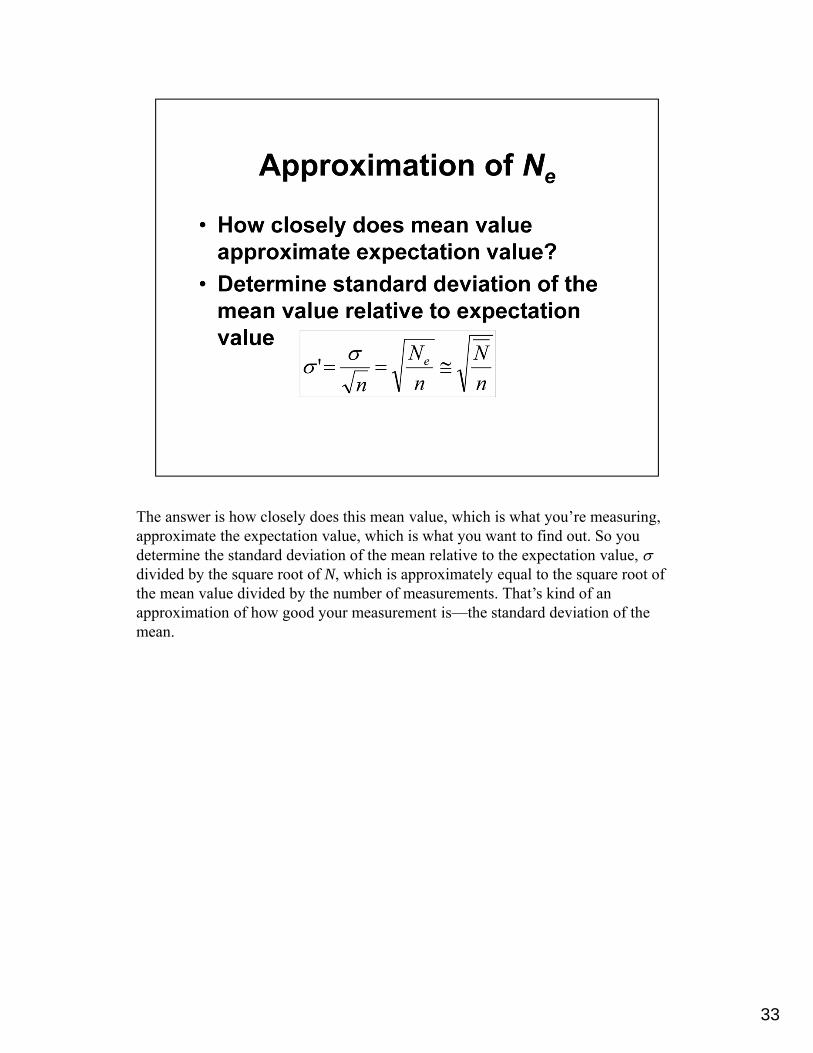
The answer is how closely does this mean value, which is what you’re measuring, approximate the expectation value, which is what you want to find out. So you determine the standard deviation of the mean relative to the expectation value, divided by the square root of N, which is approximately equal to the square root of the mean value divided by the number of measurements. That’s kind of an approximation of how good your measurement is—the standard deviation of the mean.

33

Percent standard deviation of the mean is approximately equal to 100 divided by the square root of the total number of events detected in all N measurements. Most of what we are doing has to deal with measurements, and we have to recognize that anytime we’re doing a measurement, there is a certain level of uncertainty in our measurements. We want to try to minimize what that certain level of uncertainty is. So you are going to see this treatment being repeated probably in your Medical Physics III course when you will be measuring the output of linear accelerators, and in your Radiation Detection course when you really will be focusing in on the whole concept of measurement.

34

The standard deviation is often confused with the standard deviation of the mean.

A standard deviation is based on the assumption that the distribution of data is truly random. In reality most measured data is not truly random since we take a sample of the data. If we perform an experiment and obtain some data, we will obtain a mean value of the data, but if we repeat the experiment, we may obtain a slightly different mean value. If we build a distribution, not of the raw data, but of the mean values, we will find that the distribution has a standard deviation, which is the standard deviation of the mean.

The standard deviation of the mean is often considered a better indicator of the precision of a set of measurements.

An excellent description of the difference between standard deviation and standard deviation of the mean can be found in this YouTube video: http://www.youtube.com/watch?v=MKnclPpnslg

35

Let us conclude the discussion of stochastic versus deterministic by comparing stochastic effects to deterministic effects, specifically with the effects of radiation.

Some radiation effects are stochastic. These are characterized by the fact that (1) the severity of the radiation effect is independent of absorbed dose, (2) there is no dose threshold, and (3) the probability of occurrence of the effect depends on the dose. Thus the greater the dose, the more likely the effect, not the more severe the effect.

Examples of stochastic effects of radiation include radiation-induced carcinogenesis and possible genetic effects of radiation such as mutations.

Stochastic effects are primarily low-dose effects. It is conceivable that a single ionizing event could induce cancer. Highly unlikely, but still possible. Increasing the dose does not increase the severity of cancer induction, only the probability of cancer induction.

36

Other radiation effects are deterministic. For deterministic effects, the extent of radiation damage depends on the absorbed dose, and a threshold exists below which there is no damage.

Examples of deterministic effects of radiation include cataracts and erythema (skin reddening); in fact, most acute radiation effects that we see in patients undergoing radiation therapy are deterministic effects.

Erythema, for example, will not occur at very low doses of radiation. Above some threshold dose, erythema will occur, and the extent of skin reaction will increase with increased dose.

37

38

When we do measurements, we will need to differentiate between accuracy and precision.

The accuracy of a measurement is a measure of how correct is the result of the measurement; how close does the measurement approach truth. Precision says how reproducible is the result of the measurement; how close is a single measurement to the expectation value of the quantity.

We can estimate both precision and accuracy. To estimate precision if we let Ni be the value obtained as the value of a single measurement of a set of N measurements, then an estimate of precision is approximately equal to the root mean square deviation of the measured value from the average value.

39

But more important is to estimate the precision of the mean value of nmeasurements. The precision of the mean value is where you take n minus the mean value of the measurement, sum them up over all the measurements, divide by n times n-1 and take the square root. That’s an estimate of your precision.

40

Keeping that in mind, let’s do an example. Let’s do some radiation detection. Here is an example out of the Attix book.

We have a gamma ray detector with a 100% counting efficiency, so it can count every gamma ray that passes through it. We’re putting this detector in a uniform radiation field.

We make 10 measurements of equal duration. The duration of the measurement is 100 seconds, and we’re counting ionizing events, so we’re just detecting radiation and we’re not measuring the energy.

In each measurement the average number of counts of these 10 measurements is 1.00 × 105 counts. What is the mean value of count rate and what is the precision of the measurement?

41

There’s a mean value of 105 counts in each measurement, and you are doing 10 measurements. The standard deviation of the mean is approximately equal to the square root of the mean number of counts, 105, divided by the number of measurements, which is 10. So the standard deviation of the mean is 102 counts.

If we wanted to decrease that standard deviation, that is, get higher precision, we would need to take more measurements. But notice, because things go as 1 over the square root of the number of measurements, if we wanted to change the precision from 102 counts to 101 counts, we’d have to do a thousand measurements. That’s a lot of measurements. So somehow we have to strike a comfortable balance in the real world.

Now the mean is 1×105, the standard deviation of the mean is ± 102, so the count rate is the number of counts divided by the time interval or 105 ± 102 divided by 102

or 103 ± 1 count per second.

And that’s how we can determine precision.

42

However, we still are not sure that the number is accurate. The precision just tells us how reproducible the measurements are. We could have some kind of an error that causes inaccuracy.

43

44

An error is defined to be the difference between a calculated or observed value and the true value. It’s very important to recognize what the sources of error are.

There are three kinds of errors. There are illegitimate errors, there are systematic errors, and then there are random errors. It’s important to be able to recognize what the extent of these errors are. In fact, we don’t even like to use the term “error.” Error implies some kind of a mistake. Very often, it’s not a mistake you’re making, but simply an inherent uncertainty in the nature of your measurement process.

We don’t make mistakes. We sometimes do, but there are ways to catch them. We make sure we have ways to catch them. So we often prefer to call errors, especially random error, “uncertainties.”

45

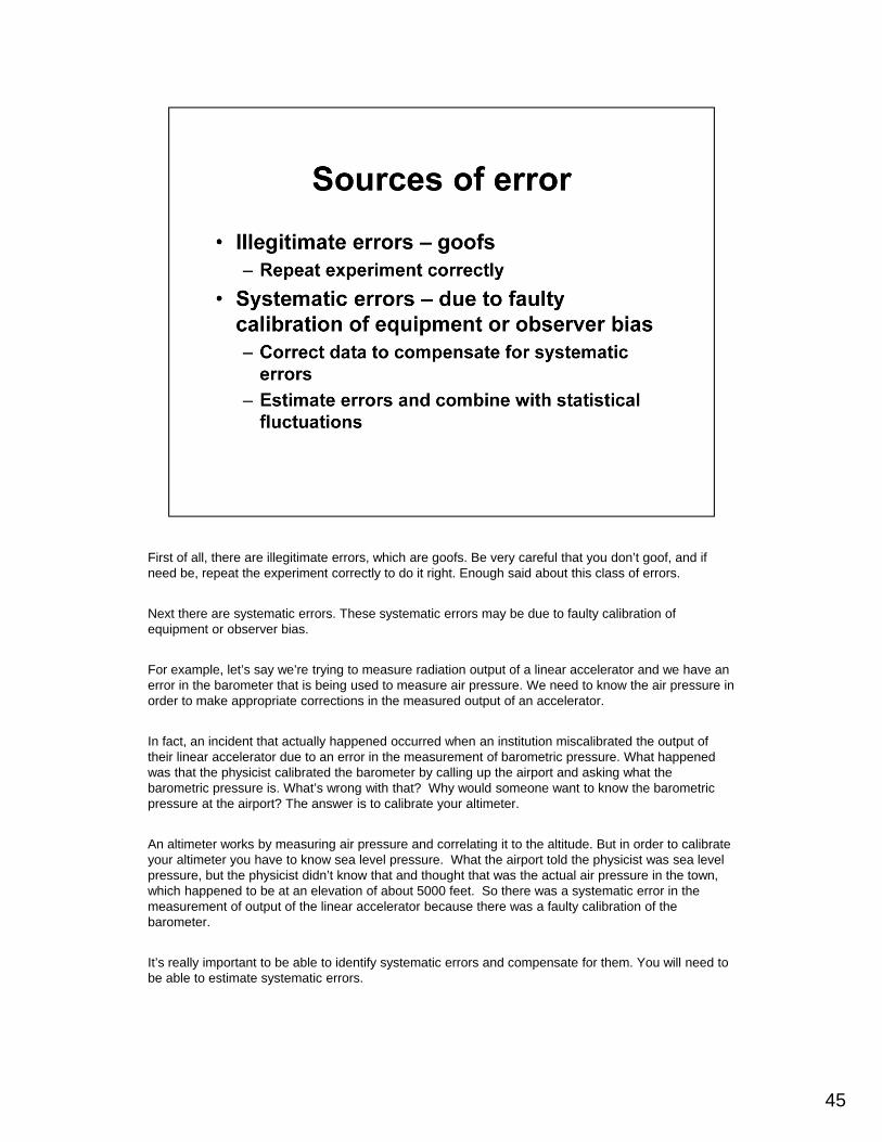
First of all, there are illegitimate errors, which are goofs. Be very careful that you don’t goof, and if need be, repeat the experiment correctly to do it right. Enough said about this class of errors.

Next there are systematic errors. These systematic errors may be due to faulty calibration of equipment or observer bias.

For example, let’s say we’re trying to measure radiation output of a linear accelerator and we have an error in the barometer that is being used to measure air pressure. We need to know the air pressure in order to make appropriate corrections in the measured output of an accelerator.

In fact, an incident that actually happened occurred when an institution miscalibrated the output of their linear accelerator due to an error in the measurement of barometric pressure. What happened was that the physicist calibrated the barometer by calling up the airport and asking what the barometric pressure is. What’s wrong with that? Why would someone want to know the barometric pressure at the airport? The answer is to calibrate your altimeter.

An altimeter works by measuring air pressure and correlating it to the altitude. But in order to calibrate your altimeter you have to know sea level pressure. What the airport told the physicist was sea level pressure, but the physicist didn’t know that and thought that was the actual air pressure in the town, which happened to be at an elevation of about 5000 feet. So there was a systematic error in the measurement of output of the linear accelerator because there was a faulty calibration of the barometer.

It’s really important to be able to identify systematic errors and compensate for them. You will need to be able to estimate systematic errors.

46

Now there are other sources of error. The other sources are random uncertainty due to the finite precision of the experiment. Ways to decrease random uncertainty would be to improve the experiment, refine your technique, and sometimes you are still left with the random uncertainty.

Very often by repeating the experiment over and over again, doing it several times, you can decrease random uncertainty.

Let me conclude our discussion of uncertainties by giving you a real-life example extracted from the dissertation of one of our former graduate students.

We want to know how accurately we can set up patients for the treatment of lung cancer. We performed a study in which we implanted inert gold markers around the tumor and imaged the patient using the radiation beam. This imaging technique is called “portal imaging.” We would then see where these implanted fiducials are. Patients are normally set up using external markings on the skin surface. So if we look at the image of the fiducials every day we can determine two quantities. First, we can determine the mean position of the fiducials, and second, we can determine the spread of the distribution of the fiducials.

The deviation of the mean fiducial position from where we think it was supposed to be on the original treatment plan is a measure of the systematic uncertainty in setting up the patient. We think we are setting up the patient in one place, but because of systematic differences in the position of the patient on the image data set used for planning, we introduced a systematic uncertainty in the patient position.

The spread of the fiducial position is the random uncertainty, and that’s something we can’t really do very much about. This uncertainty is inherent in the process of setting up a patient. In order to reduce this random uncertainty, we would have to modify the way we set up our patient.

One of the approaches proposed to reduce systematic uncertainty is to image the patient at treatment several times, determine the mean position of the tumor for these times, and re-set up the patient in that mean position. We can thus correct for systematic uncertainty, but the random uncertainty still remains.

47

So, to reduce the systematic uncertainty, we can reposition the patient, but to reduce the random uncertainty, we just cannot do that unless we use a more precise method of aligning the patient than the use of external markings.

We will have to deal with systematic uncertainties, we will have to deal with random uncertainties. The way in which one handles the two types of uncertainties is different. It is important when doing measurements to understand these types of uncertainties.

48