osmotically driven pipe flows and their relation to sugar transport in

J. Fluid Mech. (2009), vol. 636, pp. 371–396. c© Cambridge University Press 2009

doi:10.1017/S002211200900799X

371

Osmotically driven pipe flows and their relationto sugar transport in plants

KARE H. JENSEN1,2, EMMANUELLE RIO1,3,RASMUS HANSEN1, CHRISTOPHE CLANET4

AND TOMAS BOHR1†1Center for Fluid Dynamics, Department of Physics, Technical University of Denmark, Building 309,

2800 Kgs. Lyngby, Denmark2Center for Fluid Dynamics, Department of Micro- and Nanotechnology, Technical University of

Denmark, DTU Nanotech Building 345 East, 2800 Kgs. Lyngby, Denmark3Laboratoire de Physique des Solides, Univ. Paris-Sud, CNRS, UMR 8502,

F-91405 Orsay Cedex, France4IRPHE, Universites d’Aix-Marseille, 49 Rue Frederic Joliot-Curie BP 146,

F-13384 Marseille Cedex 13, France

(Received 28 May 2008; revised 28 April 2009; accepted 28 April 2009)

In plants, osmotically driven flows are believed to be responsible for translocation ofsugar in the pipe-like phloem cell network, spanning the entire length of the plant – theso-called Munch mechanism. In this paper, we present an experimental and theoreticalstudy of transient osmotically driven flows through pipes with semi-permeable walls.Our aim is to understand the dynamics and structure of a ‘sugar front’, i.e. thetransport and decay of a sudden loading of sugar in a water-filled pipe which isclosed in both ends. In the limit of low axial resistance (valid in our experimentsas well as in many cases in plants) we show that the equations of motion for thesugar concentration and the water velocity can be solved exactly by the method ofcharacteristics, yielding the entire flow and concentration profile along the tube. Theconcentration front decays exponentially in agreement with the results of Eschrich,Evert & Young (Planta (Berl.), vol. 107, 1972, p. 279). In the opposite case of verynarrow channels, we obtain an asymptotic solution for intermediate times showinga decay of the front velocity as M−1/3t−2/3 with time t and dimensionless numberM ∼ ηκL2r−3 for tubes of length L, radius r , permeability κ and fluid viscosity η. Theexperiments (which are in the small M regime) are in good quantitative agreementwith the theory. The applicability of our results to plants is discussed and it is shownthat it is probable that the Munch mechanism can account only for the short distancetransport of sugar in plants.

1. IntroductionThe translocation of sugar in plants, which takes place in the phloem sieve tubes, is

not well understood on the quantitative level. The current belief, called the pressure-flow hypothesis (Nobel 1999), is based on the pioneering work of Ernst Munch in the1920s (Munch 1930). It states, that the motion in the phloem is purely passive, due tothe osmotic pressures that build up relative to the neighbouring xylem in response to

† Email address for correspondence: [email protected]

372 K. H. Jensen, E. Rio, R. Hansen, C. Clanet and T. Bohr

Sinks

Fruit

Sink

10–50 μm

0.1–3 mm

Sugar

Sieve plates

Semi-permeablecell wall

Phloem Xylem

Xylem

Sources

Phloem

(a)

(b)

Figure 1. In plants, two separate pipe-like systems are responsible for the transport of waterand sugar. The xylem conducts water from the roots to the shoot while the phloem conductssugar and other nutrients from places of production to places of growth and storage. Themechanism believed to be responsible for sugar translocation in the phloem, called the Munchmechanism or the pressure-flow hypothesis (Nobel 1999), states the following: As sugar isproduced via photosynthesis in sources it is actively loaded into the tubular phloem cells. Asit enters the phloem, the chemical potential of the water inside is lowered compared to thesurrounding tissue, thereby creating a net flux of water into the phloem cells. This influx ofwater in turn creates a bulk flow of sugar and water towards the sugar sink shown in (b),where active unloading takes place. As the sugar is removed, the chemical potential of thewater inside the phloem is raised resulting in a flow of water out of the sieve element.

loading and unloading of sugar in different parts of the plant, as shown in figure 1.This mechanism is much more effective than diffusion, since the osmotic pressuredifferences caused by different sugar concentrations in the phloem create a bulk flowdirected from large concentrations to small concentrations, in accordance with thebasic need of the plant. Such flows are often called osmotically driven pressure flows(Thompson & Holbrook 2003), or osmotically driven volume flows (Eschrich, Evert &Young 1972).

To study the osmotically driven flows, Eschrich et al. (1972) conducted simple modelexperiments. Their set-up consisted of a semi-permeable membrane tube submergedin a water reservoir, modelling a phloem sieve element and the surrounding water-filled tissue. At one end of the tube a solution of sugar, water and dye was introducedto mimic the sudden loading of sugar into a phloem sieve element. In the case ofthe closed tube, they found that the sugar front velocity decayed exponentially in

Osmotically driven pipe flows and their relation to sugar transport in plants 373

time as it approached the far end of the tube. Also, they found the initial velocity ofthe sugar front to be proportional to concentration of the sugar solution. Throughsimple conservation arguments, they showed that for a flow driven according to thepressure-flow hypothesis, the velocity of the sugar front is given by

uf =L

t0exp

(− t

t0

)where t0 =

r

2κΠ, (1.1)

where t is time, L is the length of the sieve element and r its radius, κ is thepermeability of the membrane and Π is the osmotic pressure of the sugar solution.For dilute solutions, Π ≈ RT c (Landau & Lifshitz 1980), where R is the gas constant,T the absolute temperature and c the concentration in moles per volume. Theconservation argument for (1.1) is the following: for incompressible flow in a widerigid semi-permeable tube of length L imbedded in water, we imagine part of the tubeinitially filled with sugar solution and the rest with pure water. For a wide tube withslow flow, viscous effects and thus the pressure gradient along the tube is negligibleand the pressure is simply equal to the osmotic pressure Π averaged over the tube,i.e. RT c where c is the constant average sugar concentration. The water (volume)flux through the part of the tube ahead of the sugar front xf (where there is noosmosis) is −2πrκRT c(L − xf ), where κ is the permeability of the tube and the flowis negative since water flows out. This will be equal to the rate of change of volumeahead of xf and thus, due to incompressibility, is equal to −πr2dxf /dt . Putting thesetwo expressions together we get

dxf

dt=

2LpRT c

r(L − xf ) =

1

t0(L − xf ) (1.2)

leading to uf = dxf /dt given by (1.1).In the experiments performed by Eschrich et al. (1972) good qualitative agreement

with (1.1) was obtained, but on the quantitative level the agreement was rather poor.We thus chose to perform independent experiments along the same lines. Eschrich etal. (1972) used dye to track the sugar, and in one of our set-ups we can check thismethod by directly following the sugar without using dye. Also, we make independentmeasurements of the membrane properties, which then allow detailed comparison withthe predictions showing good quantitative agreement.

Simultaneously with the experiments, we develop the theory for osmotic flows. Theabove derivation of the front propagation is simplified by the lack of viscosity anddiffusion and, indeed, by the very assumption that a well-defined sugar front exists. Togo beyond this we must use the coupled equations for the velocity and concentrationfields as they vary along the tubes and in time. Here we follow the footsteps of a largenumber of authors, as discussed later. Our main contribution is the analysis of thedecay of an initially localized sugar concentration in a channel closed in both endsdescribed by (4.9) and (4.10). Here we point out that the main dimensionless number(termed as Munch number) can be chosen as

M =16ηL2κ

r3, (1.3)

where η is the fluid viscosity. We show how to simplify the equations and obtain exactsolutions in the regimes M � 1 (the regime of the experiments in this paper and ofthose of Eschrich et al.) and asymptotic solutions for M � 1. Both regimes are foundin plants and we propose an effective way for numerical integration of the equationsin the general case using Green’s functions. In the regime M � 1 the solubility of the


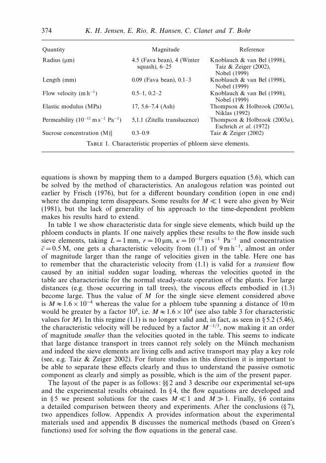
Quantity Magnitude Reference

Radius (μm) 4.5 (Fava bean), 4 (Winter Knoblauch & van Bel (1998),squash), 6–25 Taiz & Zeiger (2002),

Nobel (1999)Length (mm) 0.09 (Fava bean), 0.1–3 Knoblauch & van Bel (1998),

Nobel (1999)Flow velocity (m h−1) 0.5–1, 0.2–2 Knoblauch & van Bel (1998),

Nobel (1999)Elastic modulus (MPa) 17, 5.6–7.4 (Ash) Thompson & Holbrook (2003a),

Niklas (1992)Permeability (10−11 m s−1 Pa−1) 5,1.1 (Zitella translucence) Thompson & Holbrook (2003a),

Eschrich et al. (1972)Sucrose concentration (M)] 0.3–0.9 Taiz & Zeiger (2002)

Table 1. Characteristic properties of phloem sieve elements.

equations is shown by mapping them to a damped Burgers equation (5.6), which canbe solved by the method of characteristics. An analogous relation was pointed outearlier by Frisch (1976), but for a different boundary condition (open in one end)where the damping term disappears. Some results for M � 1 were also given by Weir(1981), but the lack of generality of his approach to the time-dependent problemmakes his results hard to extend.

In table 1 we show characteristic data for single sieve elements, which build up thephloem conducts in plants. If one naively applies these results to the flow inside suchsieve elements, taking L =1 mm, r =10 μm, κ = 10−11 m s−1 Pa−1 and concentrationc =0.5 M, one gets a characteristic velocity from (1.1) of 9 mh−1, almost an orderof magnitude larger than the range of velocities given in the table. Here one hasto remember that the characteristic velocity from (1.1) is valid for a transient flowcaused by an initial sudden sugar loading, whereas the velocities quoted in thetable are characteristic for the normal steady-state operation of the plants. For largedistances (e.g. those occurring in tall trees), the viscous effects embodied in (1.3)become large. Thus the value of M for the single sieve element considered aboveis M ≈ 1.6 × 10−4 whereas the value for a phloem tube spanning a distance of 10 mwould be greater by a factor 108, i.e. M ≈ 1.6 × 104 (see also table 3 for characteristicvalues for M). In this regime (1.1) is no longer valid and, in fact, as seen in § 5.2 (5.46),the characteristic velocity will be reduced by a factor M−1/3, now making it an orderof magnitude smaller than the velocities quoted in the table. This seems to indicatethat large distance transport in trees cannot rely solely on the Munch mechanismand indeed the sieve elements are living cells and active transport may play a key role(see, e.g. Taiz & Zeiger 2002). For future studies in this direction it is important tobe able to separate these effects clearly and thus to understand the passive osmoticcomponent as clearly and simply as possible, which is the aim of the present paper.

The layout of the paper is as follows: §§ 2 and 3 describe our experimental set-upsand the experimental results obtained. In § 4, the flow equations are developed andin § 5 we present solutions for the cases M � 1 and M � 1. Finally, § 6 containsa detailed comparison between theory and experiments. After the conclusions (§ 7),two appendices follow. Appendix A provides information about the experimentalmaterials used and appendix B discusses the numerical methods (based on Green’sfunctions) used for solving the flow equations in the general case.


pt

ber

gt

(a)

(b)

spm

10 mm

spm

gtsswr

30 mmss

l

L30 cm

wr

sc

ds

rs

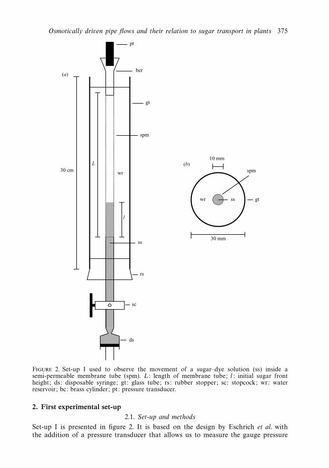
Figure 2. Set-up I used to observe the movement of a sugar–dye solution (ss) inside asemi-permeable membrane tube (spm). L: length of membrane tube; l: initial sugar frontheight; ds: disposable syringe; gt: glass tube; rs: rubber stopper; sc: stopcock; wr: waterreservoir; bc: brass cylinder; pt: pressure transducer.

2. First experimental set-up2.1. Set-up and methods

Set-up I is presented in figure 2. It is based on the design by Eschrich et al. withthe addition of a pressure transducer that allows us to measure the gauge pressure


1 2 3 4 5

Mean sugar concentration, c (mM) 1.5 ± 0.3 2.10 ± 0.03 2.4 ± 0.2 4.2 ± 0.7 6.8 ± 0.1Osmotic pressure, Π (bar) 0.14 ± 0.02 0.15 ± 0.01 0.31 ± 0.03 0.39 ± 0.01 0.68 ± 0.02Membrane tube length, L (cm) 28.5 20.8 28.5 28.5 20.6Initial front height, l (cm) 4.9 3.7 6.6 6.5 4.8

Table 2. Data for the experimental runs shown in figure 3.

(which is what we from now on will refer to as ‘pressure’) inside the membrane tubecontinuously. More precisely, it consisted of a 30 cm long, 30 mm wide glass tube inwhich a semi-permeable membrane tube of equal length and a diameter of 10 mm wasinserted. At one end, the membrane tube was fitted over a glass stopcock equippedwith a rubber stopper. On the other end, the membrane tube was fitted over a brasscylinder equipped with a holder to accommodate a pressure transducer for measuringthe pressure inside the membrane tube.

After filling the 30 mm wide glass tube with water, water was pressed into thesemi-permeable tube with a syringe. Care was taken so that no air bubbles werestuck inside the tube. For introducing the sugar solution into the tube, a syringe wasfilled with the solution and then attached to the lower end of the stopcock which waskept closed. After fitting the syringe, the stopcock was opened and the syringe pistonwas very slowly pressed in, until a suitable part of the tube had been filled with thesolution. Care was also taken to avoid any mixing between the sugar solution andthe water already present in the semi-permeable tube. The physical characteristics ofthe membranes and of the sugar we used are discussed in appendix A. To track themovement of the sugar solution it was mixed with a red dye and data was recordedby taking pictures of the membrane tube at intervals of 15 min using a digitalcamera.

2.2. Experimental results obtained with set-up I

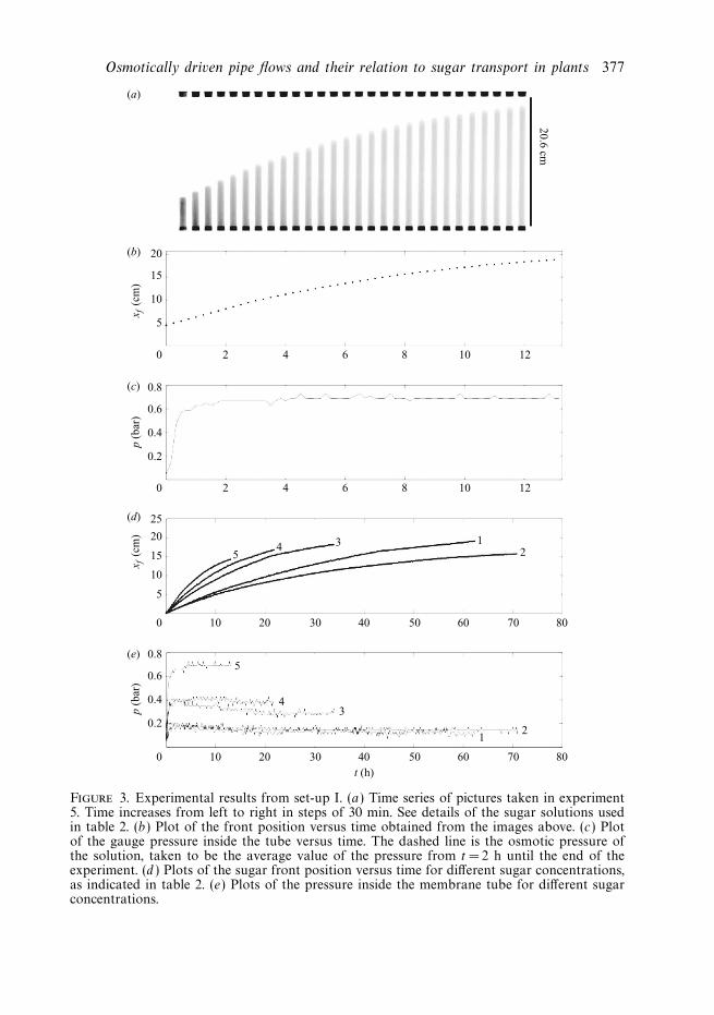
An example of a set of data is shown in figure 3. In figure 3(a) are the raw images,which after processing give figure 3(b) showing the position of the sugar front, xf ,as a function of time. The error bars on xf are estimated to be ±1 mm, but are toosmall to be seen. Finally, figure 3(c) shows the pressure inside the tube as a functionof time. At first, a linear motion of the front is observed with a front velocity of∼ 1 cmh−1. This is then followed by a decrease in the front velocity as the frontapproaches the end of the tube. The pressure is seen to rise rapidly during the firsthour before settling to a constant value, indicated by the dashed line. This constantvalue is taken to be the osmotic pressure Π of the sugar solution. Looking at figure3(a), one observes that diffusion has the effect of dispersing the front slightly astime passes. Below the front, the concentration seems to be uniform throughout thecross-section of the tube, and there is no indication of large boundary layers formingnear the membrane walls.

Similar experiments with different sugar concentrations were made and a plot of theresults can be seen in figure 3(d,e). The experimental conditions for the five differentsets of experiments are given in table 2. Qualitatively the motion of the front and thepressure increase follows the same pattern. One notices that the speed with which thefronts move is related to the mean sugar concentration inside the membrane tube,with the high-concentration solutions moving faster than the low-concentration ones.


20

15

10

5

0 42

t (h)

6 8 10 12

20.6

cm

0 42

10 20 30 40 50 60 70 80

6 8 10 12

x f (

cm)

25

20

15

10

5

5

5

43

21

413

2

0

10 20 30 40 50 60 70 800

x f (

cm)

0.8

0.6

0.4

0.2

p (b

ar)

0.8

0.6

0.4

0.2

p (b

ar)

(a)

(b)

(c)

(d)

(e)

Figure 3. Experimental results from set-up I. (a) Time series of pictures taken in experiment5. Time increases from left to right in steps of 30 min. See details of the sugar solutions usedin table 2. (b) Plot of the front position versus time obtained from the images above. (c) Plotof the gauge pressure inside the tube versus time. The dashed line is the osmotic pressure ofthe solution, taken to be the average value of the pressure from t = 2 h until the end of theexperiment. (d ) Plots of the sugar front position versus time for different sugar concentrations,as indicated in table 2. (e) Plots of the pressure inside the membrane tube for different sugarconcentrations.


(a)sg

sg

sg

Prism-

Top view

Side view

z

y

x

y

30 cm

7 cm

5 cm

Screen(b)

Semi-permeable membrane

Las

er s

heet

Water reservoir

Sugar solution

Water

Water reservoir

Water

Sugar solution

- Semi-permeable membrane

Water reservoir

x

y

z

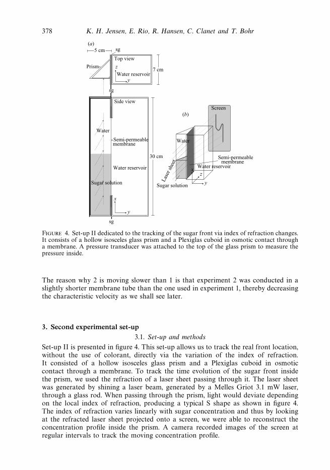
Figure 4. Set-up II dedicated to the tracking of the sugar front via index of refraction changes.It consists of a hollow isosceles glass prism and a Plexiglas cuboid in osmotic contact througha membrane. A pressure transducer was attached to the top of the glass prism to measure thepressure inside.

The reason why 2 is moving slower than 1 is that experiment 2 was conducted in aslightly shorter membrane tube than the one used in experiment 1, thereby decreasingthe characteristic velocity as we shall see later.

3. Second experimental set-up3.1. Set-up and methods

Set-up II is presented in figure 4. This set-up allows us to track the real front location,without the use of colorant, directly via the variation of the index of refraction.It consisted of a hollow isosceles glass prism and a Plexiglas cuboid in osmoticcontact through a membrane. To track the time evolution of the sugar front insidethe prism, we used the refraction of a laser sheet passing through it. The laser sheetwas generated by shining a laser beam, generated by a Melles Griot 3.1 mW laser,through a glass rod. When passing through the prism, light would deviate dependingon the local index of refraction, producing a typical S shape as shown in figure 4.The index of refraction varies linearly with sugar concentration and thus by lookingat the refracted laser sheet projected onto a screen, we were able to reconstruct theconcentration profile inside the prism. A camera recorded images of the screen atregular intervals to track the moving concentration profile.


t →

5 10 150

0.2

0.4

0.6

0.8

1.0

(a)

(b)

(d) (e) ( f)

(c)

x (cm)

c (1

/c0)

5 10 150

0.2

0.4

0.6

x (cm)

dc/

dx

[1/(

c 0 c

m)]

0 10 20 30 4010

12

14

16

18

20

Time (days)

x (c

m)

5 100

0.1

0.2

0.3

0.4

0.5

Pre

ssure

(bar

)

Time (h)32 34 36

0

0.1

0.2

0.3

0.4

0.5

Time (days)

Pre

ssure

(bar

)

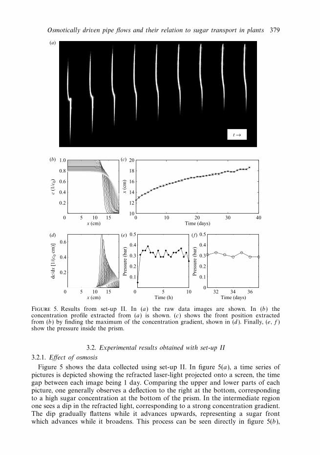
Figure 5. Results from set-up II. In (a) the raw data images are shown. In (b) theconcentration profile extracted from (a) is shown. (c) shows the front position extractedfrom (b) by finding the maximum of the concentration gradient, shown in (d ). Finally, (e, f )show the pressure inside the prism.

3.2. Experimental results obtained with set-up II

3.2.1. Effect of osmosis

Figure 5 shows the data collected using set-up II. In figure 5(a), a time series ofpictures is depicted showing the refracted laser-light projected onto a screen, the timegap between each image being 1 day. Comparing the upper and lower parts of eachpicture, one generally observes a deflection to the right at the bottom, correspondingto a high sugar concentration at the bottom of the prism. In the intermediate regionone sees a dip in the refracted light, corresponding to a strong concentration gradient.The dip gradually flattens while it advances upwards, representing a sugar frontwhich advances while it broadens. This process can be seen directly in figure 5(b),


2 4 6 8 10 120

5

10

15

x (cm)

|dc/

dx|

(m

M c

m–1)

0 20 40 60 80 100 120 1404

5

6

7

t (h)

x f (c

m)

0 2 4 6 8 10 12

5

10

15(a)

(b)

(c)

x (cm)

c (m

M)

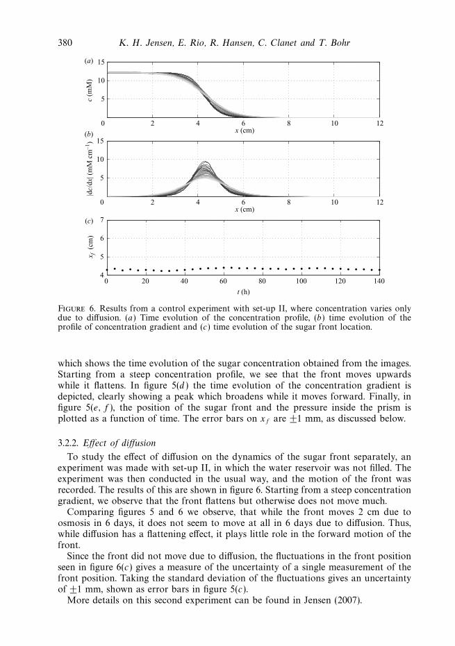
Figure 6. Results from a control experiment with set-up II, where concentration varies onlydue to diffusion. (a) Time evolution of the concentration profile, (b) time evolution of theprofile of concentration gradient and (c) time evolution of the sugar front location.

which shows the time evolution of the sugar concentration obtained from the images.Starting from a steep concentration profile, we see that the front moves upwardswhile it flattens. In figure 5(d ) the time evolution of the concentration gradient isdepicted, clearly showing a peak which broadens while it moves forward. Finally, infigure 5(e, f ), the position of the sugar front and the pressure inside the prism isplotted as a function of time. The error bars on xf are ±1 mm, as discussed below.

3.2.2. Effect of diffusion

To study the effect of diffusion on the dynamics of the sugar front separately, anexperiment was made with set-up II, in which the water reservoir was not filled. Theexperiment was then conducted in the usual way, and the motion of the front wasrecorded. The results of this are shown in figure 6. Starting from a steep concentrationgradient, we observe that the front flattens but otherwise does not move much.

Comparing figures 5 and 6 we observe, that while the front moves 2 cm due toosmosis in 6 days, it does not seem to move at all in 6 days due to diffusion. Thus,while diffusion has a flattening effect, it plays little role in the forward motion of thefront.

Since the front did not move due to diffusion, the fluctuations in the front positionseen in figure 6(c) gives a measure of the uncertainty of a single measurement of thefront position. Taking the standard deviation of the fluctuations gives an uncertaintyof ±1 mm, shown as error bars in figure 5(c).

More details on this second experiment can be found in Jensen (2007).


S

Ar

0 xi–lΔx

xf xi–l L

Water reservoir

Semi-permeable membrane

Sugar

Water flux

Figure 7. Sketch of the tube.

4. Theoretical analysis4.1. Front propagation via flow equations

The equations of motion for osmotically driven flows have been derived and analysedthoroughly several times in the literature (Weir 1981) and have been studied carefullynumerically (Henton 2002; Thompson & Holbrook 2003a, b). For the sake ofcompleteness, we shall include a short derivation of these.

We consider a tube of length L and radius r , as shown in figure 7. The tubehas a constant cross-section of area A= πr2 and circumference S = 2πr and its wallsare made of a semi-permeable membrane with permeability κ . Inside the tube is asolution of sugar in water with concentration c(x) = c(x, t). Throughout this paper,we study the transient dynamics generated by an asymmetrical initial concentrationdistribution, where the sugar is initially localized to one end of the tube with aconcentration level c0. The tube is surrounded by a water reservoir, modelling thewater surrounding the membrane tube in set-up I.

We shall assume that L � r and that the radial component of the flow velocityinside the tube is much smaller than the axial component, as is indeed the casein the experiments. With these assumptions, we will model the flow in the spirit oflubrication theory and consider only a single average axial velocity component u(x, t).Also, we will assume that the concentration c is independent of the radial position ρ

an assumption that can be verified experimentally in set-up II.Let us now consider the equation for volume conservation by looking at a small

section of the tube between xi−1 and xi . The volume flux into the section due toadvection is

A(ui−1 − ui), (4.1)

where the axial flow velocities are taken to be ui−1 and ui at xi−1 and xi , respectively.The volume flux inwards across the membrane due to osmosis (Schultz 1980) is

S�xκ(RT c(x, t) − p(x, t)), (4.2)

where p is the local difference of pressure across the membrane and c is the localconcentration. For clarity we use the van’t Hoff value Π = RT c for the osmoticpressure, which is valid only for dilute (ideal) solutions. In appendix A.3, we show thatthe linear relation between Π and c is verified experimentally as Π = (0.1 ± 0.01 barmM−1)c. Assuming conservation of volume, we get

A(ui−1 − ui) + S�xκ(RT c − p) = 0. (4.3)


Letting �x → 0 and using that the cross-section to perimeter ratio reduces to r/2, thisbecomes

r

2

∂u

∂x= κ(RT c − p). (4.4)

For these very slow and slowly varying flows, the time dependence of the Navier–Stokes equation can be neglected and the velocity field is determined by theinstantaneous pressure gradient through the Poiseuille or Darcy relation (for a circulartube)

u = − r2

8η

∂p

∂x, (4.5)

where η is the dynamic viscosity of the solution, typically ∼ 1.5 × 10−3 Pa s in ourexperiments.

Differentiating (4.4) with respect to x and inserting the result from (4.5) we get forthe conservation of water that

RT∂c

∂x=

r

2κ

∂2u

∂x2− 8η

r2u. (4.6)

The final equation expresses the conservation of sugar advected with velocity u anddiffusing with molecular diffusivity D

∂c

∂t+

∂uc

∂x= D

∂2c

∂x2. (4.7)

The set of equations (4.6) and (4.7) is equivalent to those of Thompson & Holbrook(2003b) except for the fact that we have removed the pressure by substitution, andthat we do not consider elastic deformations of the tube.

4.1.1. Non-dimensionalization of the flow equations

To non-dimensionalize (4.6) and (4.7), we introduce the following scaling

c = c0C, u = u0U, x = LX, t = t0τ,

L has been chosen such that the spatial domain is now of the unit interval X ∈ [0, 1],u0 = L/t0 and c0 is the initial concentration level in one end of the tube. Choosingfurther

t0 =r

2κRT c0

, M =16ηL2κ

r3and D =

D

u0L=

Dr

2RT c0L2κ, (4.8)

and inserting in (4.6) and (4.7), we get the non-dimensional flow equations

∂2U

∂X2− MU =

∂C

∂X, (4.9)

∂C

∂τ+

∂UC

∂X= D

∂2C

∂X2. (4.10)

The parameter M corresponds to the ratio of axial to membrane flow resistance,which we shall refer to as the Munch number. This is identical to the parameter F inThompson & Holbrook (2003b). The second parameter D is the Peclet number. Thus,the longer the tube the less important the diffusion becomes and the more importantthe pressure gradient due to viscous effects becomes.

Values of the parameters M and D in different situations can be seen in table 3.The typical magnitude of the parameters M and D in plants are found from the


M D

Set-up I 2 × 10−8 6 × 10−5

Set-up II 10−9 2 × 10−2

Single sieve element (L= 1 mm) 5 × 10−4 5 × 10−4

Leaf (L= 1 cm) 5 × 10−2 5 × 10−5

Branch (L = 1 m) 5 × 102 5 × 10−7

Small tree (L = 10 m) 5 × 104 5 × 10−8

Table 3. Values of the parameters M and D in various situations.

following values (also given in table 3):

r = 10 μm, η = 1.5 × 10−3 Pa s, u0 = 2 m h−1, κ = 2 × 10−11 m (Pa s)−1.

We observe, that M and D are small in both experiments, and that for short distancetransport in plants this is also the case. However, over length scales comparable to abranch (L = 1 m) or a small tree (L = 10 m) M is large, so in this case the pressuregradient is not negligible.

When deriving the equations for osmotically driven flows, we have assumed thatthe concentration inside the tube was a function of x and t only. However, the realconcentration inside the tube will also depend on the radial position ρ in the formof a concentration boundary layer near the membrane, in the literature called anunstirred layer (Pedley 1983). Close to the membrane, the concentration cm is loweredcompared to the bulk value cb because sugar is advected away from the membraneby the influx of water. This, in turn, results in a lower influx of water, ultimatelycausing the axial flow inside the tube to be slower than expected. In our experimentswe see no signs of such boundary layers and apparently their width and their effecton the bulk flow are very small.

5. Solutions of the flow equationsWe will now analyse (4.9) and (4.10). We will show that they can be solved quite

generally for M = D = 0 by the method of characteristics. For an arbitrary initialcondition, this method will generally yield an implicit solution.

For arbitrary values of M and D, we cannot solve the equations of motionanalytically and thus have to incorporate numerical methods. This topic has been thefocus of much work both in the steady-state case (Thompson & Holbrook 2003a)and in the transient case (Henton 2002). However, no formulation fully exploiting thepartially linear character of the equations capable of handling all different boundaryconditions has so far been presented. Therefore, we show that using Green’s functions,the equations of motion can be transformed into a single integro-differential equation,which can be solved using standard numerical methods with very high precision. Thistechnical numerical part is detailed in appendix B.

5.1. Results for small Munch number

In the limit M = D =0 the equations become

∂2U

∂X2=

∂C

∂X, (5.1)

∂C

∂τ+

∂UC

∂X= 0. (5.2)


By integrating (5.1) with respect to X, we get

∂U

∂X= C + F (τ ). (5.3)

If we choose U (0) = U (1) = 0, F (τ ) becomes

F (τ ) = −∫ 1

0

C dX ≡ −C(τ ). (5.4)

Using (5.3) in (5.2) gives

∂

∂X

[∂U

∂τ+ U

(∂U

∂X+ C

)]= −dC

dτ= 0, (5.5)

where the last equality follows from integrating X from 0 to 1, observing that allterms in the square bracket vanish at the end points due to the boundary conditionu(X =0, τ ) = u(X = 1, τ ) = 0. Thus C is a constant in time since the tube is closed.Integrating with respect to X and using the boundary conditions on U , this becomes

∂U

∂τ+ U

∂U

∂X= −CU. (5.6)

Equation (5.6) is a damped Burgers equation (Gurbatov, Malakhov & Saichev 1991),which can be solved using Riemann’s method of characteristics. The characteristicequations are

dU

dτ= −CU (5.7)

dX

dτ= U. (5.8)

Equation (5.7) has the solution

U = U0(ξ ) exp(−Cτ ), (5.9)

where the parametrization ξ (X, τ ) of the initial velocity has to be found from

X = ξ +1

CU0(ξ )(1 − exp(−Cτ )), (5.10)

where ξ = X at τ =0.

5.1.1. Exact solutions for simple initial conditions

An experimental condition close to that of our experiments is to use a Heavisidestep function as initial condition on C, making C initially constant in some interval[0, λ]

C(X, τ = 0) = CIH (λ − X) =

{CI for 0 � X � λ.

0 for λ < X � 1.(5.11)

Equation (5.3) now enables us to find the initial condition on the velocity

U (X, τ = 0) =

∫ X

0

(C(X′, 0) − C) dX′ =

∫ X

0

(C(X′, 0) − λCI ) dX′ (5.12)

=

{(CI − C)X for 0 � X � λ.

C(1 − X) for λ < X � 1.(5.13)


From (5.13), we have

U0(ξ ) =

{(CI − C)ξ for 0 � ξ � λ.

C(1 − ξ ) for λ < ξ � 1.(5.14)

Then, solving for ξ (X, τ ) in (5.10) gives

ξ (X, τ ) =

⎧⎪⎪⎨⎪⎪⎩

X

1 + (1/λ)(1 − λ)(1 − exp(−Cτ )for X ∈ I1,

X − 1 + exp(−Cτ )

exp(−Cτ )for X ∈ I2,

(5.15)

where the intervals I1 and I2 are defined by

I1 = [0, 1 − (1 − λ) exp(−Cτ )], (5.16)

I2 = [1 − (1 − λ) exp(−Cτ ), 1]. (5.17)

Finally, U (X, τ ) is calculated from (5.9)

U (X, τ ) =

⎧⎪⎨⎪⎩

(CI − C) exp(−Cτ )X

(1/λ)(1 − λ)(1 − exp(−Cτ ))for X ∈ I1,

C(1 − X) for X ∈ I2,

(5.18)

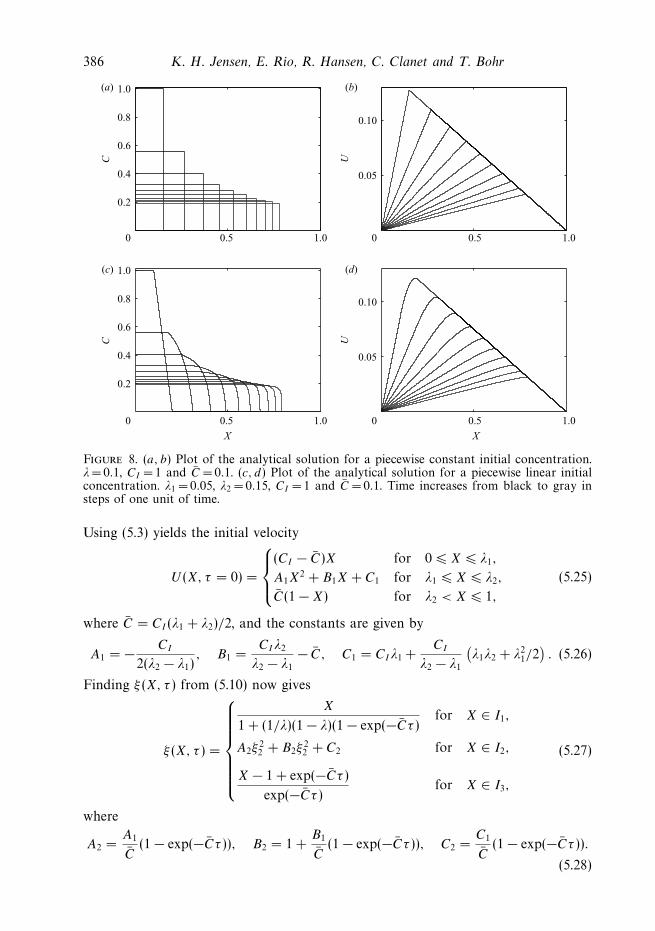
which is equivalent to the result obtained by Weir (1981). The solution is plotted infigure 8(a, b). We can now calculate the instantaneous sugar front position Xf andvelocity Uf using the right boundary of I1 from (5.16)

Xf (τ ) = 1 − (1 − λ) exp(−Cτ ), (5.19)

Uf (τ ) =dXf

dτ= C(1 − λ) exp(−Cτ ). (5.20)

Similarly, C(X, τ ) is given by

C(X, τ ) =C

1 − (1 − λ) exp(−Cτ )H (Xf − X). (5.21)

Going back to dimensional variables, (5.19) and (5.20) become

xf (t) = L − (L − l) exp(

− t

t 0

)and (5.22)

uf (t) =L

t0exp

(− t

t0

), (5.23)

where L is the length of the membrane tube, l is the initial front position and thedecay time t0 is in accordance with the simple argument given in § 1.

As noted earlier we can use the method of characteristics on arbitrary initialconditions, including the more realistic case, where the initial jump in concentrationis replaced by a continuous variation, say, a linear decrease from CI to 0 taking placebetween λ1 and λ2, i.e.

C(X, τ = 0) =

⎧⎪⎪⎨⎪⎪⎩

CI for 0 � X � λ1.

CI

λ2 − X

λ2 − λ1

for λ1 � X � λ2.

0 for λ2 < X � 1.

(5.24)


0.5 1.00

0.2

0.4

0.6

0.8

1.0(a) (b)

(c) (d)

0.5 1.00

0 00.5 1.0

X

0.5 1.0

X

C

0.05

0.10

U

0.2

0.4

0.6

0.8

1.0

C

0.05

0.10

U

Figure 8. (a, b) Plot of the analytical solution for a piecewise constant initial concentration.λ=0.1, CI = 1 and C = 0.1. (c, d) Plot of the analytical solution for a piecewise linear initialconcentration. λ1 = 0.05, λ2 = 0.15, CI = 1 and C = 0.1. Time increases from black to gray insteps of one unit of time.

Using (5.3) yields the initial velocity

U (X, τ = 0) =

⎧⎪⎨⎪⎩

(CI − C)X for 0 � X � λ1,

A1X2 + B1X + C1 for λ1 � X � λ2,

C(1 − X) for λ2 < X � 1,

(5.25)

where C = CI (λ1 + λ2)/2, and the constants are given by

A1 = − CI

2(λ2 − λ1), B1 =

CIλ2

λ2 − λ1

− C, C1 = CIλ1 +CI

λ2 − λ1

(λ1λ2 + λ2

1/2). (5.26)

Finding ξ (X, τ ) from (5.10) now gives

ξ (X, τ ) =

⎧⎪⎪⎪⎪⎪⎪⎨⎪⎪⎪⎪⎪⎪⎩

X

1 + (1/λ)(1 − λ)(1 − exp(−Cτ )for X ∈ I1,

A2ξ22 + B2ξ

22 + C2 for X ∈ I2,

X − 1 + exp(−Cτ )

exp(−Cτ )for X ∈ I3,

(5.27)

where

A2 =A1

C(1 − exp(−Cτ )), B2 = 1 +

B1

C(1 − exp(−Cτ )), C2 =

C1

C(1 − exp(−Cτ )).

(5.28)


Here

ξ2 =−B2 +

√B2

2 − 4A2(C2 − X)

2A2

, (5.29)

where the plus solution has been chosen to ensure that ξ → X as τ → 0. Finally,

I1 =

[0, λ1 +

λ1

C(CI − C)(1 − exp(−Cτ ))

], (5.30)

I2 =

[λ1 +

λ1

C(CI − C)(1 − exp(−Cτ )), 1 + (λ2 − 1) exp(−Cτ )

], (5.31)

I3 =[1 + (λ2 − 1) exp(−Cτ ), 1

]. (5.32)

Plugging into (5.9) gives U (X, τ ) as

U (X, τ ) =

⎧⎪⎪⎪⎨⎪⎪⎪⎩

(CI − C) exp(−C)X

1 + (1/λ)(1 − λ)(1 − exp(−Cτ )for X ∈ I1,(

A1ξ22 + B1ξ

22 + C1

)exp(−Cτ ) for X ∈ I2,

C (1 − X) for X ∈ I3,

(5.33)

as shown in figure 8 along with C found from (5.3), i.e.

C =∂U

∂X+ C. (5.34)

Note that the interval I2 does not shrink to 0 in time (I2 → [λ1C1/C, 1] for τ → ∞),but the curvature around the right-hand end point grows without bound so that thelimiting shape of the concentration profile again becomes a discontinuous Heavisidefunction.

5.2. Results for large Munch number

In the limit of large M � 1 we cannot neglect the pressure gradient along the channeland this term dominates the advective term in (4.9), i.e. the second derivative in U .Thus

∂C

∂X= −MU (5.35)

∂C

∂τ+

∂CU

∂X= D

∂2C

∂X2(5.36)

giving the nonlinear diffusion equation

∂C

∂τ= M−1 ∂

∂X

[C

∂C

∂X

]+ D

∂2C

∂X2. (5.37)

If we neglect molecular diffusion the resulting universal nonlinear diffusion equationcan be written as

∂C

∂τ= M−1 ∂

∂X

[C

∂C

∂X

]. (5.38)

This can be done as long as M−1C � D ≈ 10−5. If M becomes even larger normaldiffusion will take over. Equation (5.38) belongs to a class of equations which havebeen studied, e.g. in the context of intense thermal waves by Zeldovich et al. and flowthrough porous media by Barenblatt (1996) in the 1950s. The Munch number M canbe removed by rescaling the time according to τ = Mt , so when M is large we get


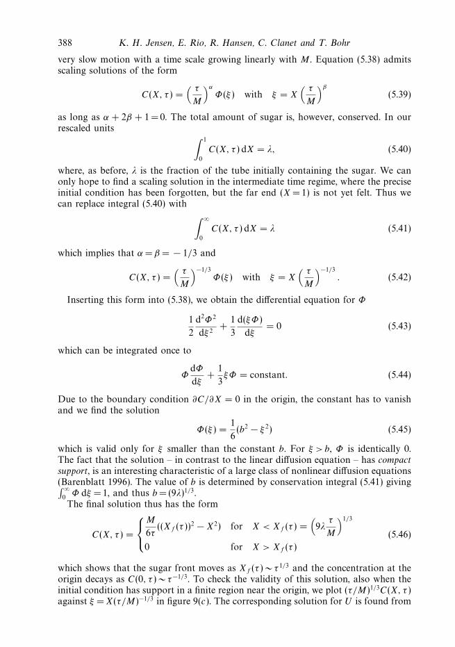
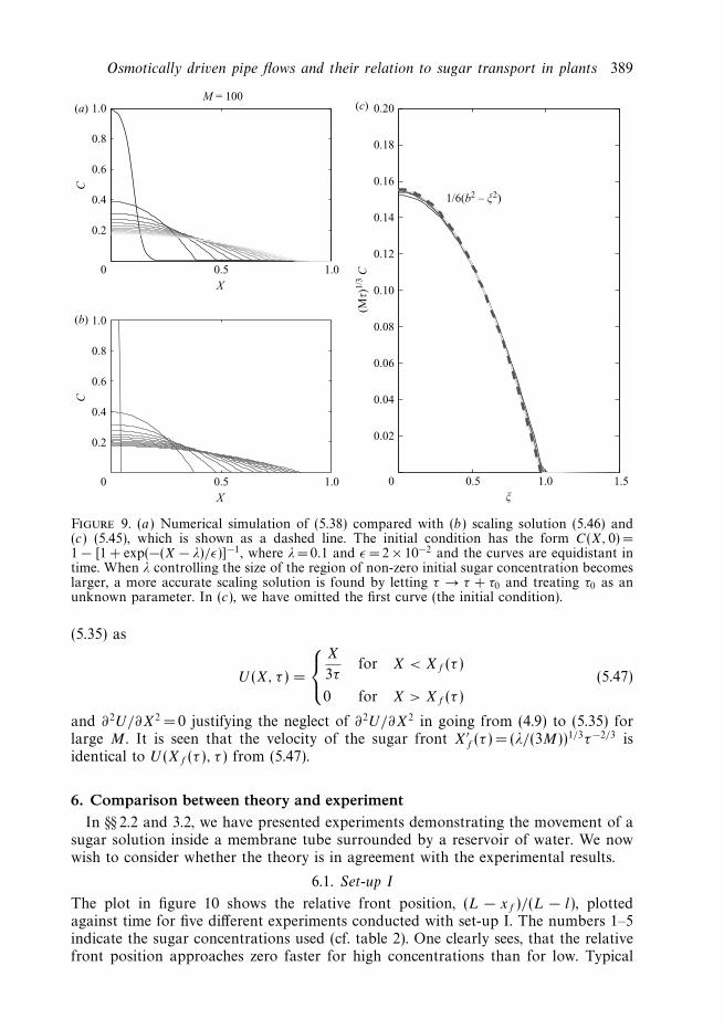
very slow motion with a time scale growing linearly with M . Equation (5.38) admitsscaling solutions of the form

C(X, τ ) =( τ

M

)α

Φ(ξ ) with ξ = X( τ

M

)β

(5.39)

as long as α + 2β + 1 = 0. The total amount of sugar is, however, conserved. In ourrescaled units ∫ 1

0

C(X, τ ) dX = λ, (5.40)

where, as before, λ is the fraction of the tube initially containing the sugar. We canonly hope to find a scaling solution in the intermediate time regime, where the preciseinitial condition has been forgotten, but the far end (X = 1) is not yet felt. Thus wecan replace integral (5.40) with ∫ ∞

0

C(X, τ ) dX = λ (5.41)

which implies that α = β = − 1/3 and

C(X, τ ) =( τ

M

)−1/3

Φ(ξ ) with ξ = X( τ

M

)−1/3

. (5.42)

Inserting this form into (5.38), we obtain the differential equation for Φ

1

2

d2Φ2

dξ 2+

1

3

d(ξΦ)

dξ= 0 (5.43)

which can be integrated once to

ΦdΦ

dξ+

1

3ξΦ = constant. (5.44)

Due to the boundary condition ∂C/∂X = 0 in the origin, the constant has to vanishand we find the solution

Φ(ξ ) =1

6(b2 − ξ 2) (5.45)

which is valid only for ξ smaller than the constant b. For ξ > b, Φ is identically 0.The fact that the solution – in contrast to the linear diffusion equation – has compactsupport, is an interesting characteristic of a large class of nonlinear diffusion equations(Barenblatt 1996). The value of b is determined by conservation integral (5.41) giving∫ ∞

0Φ dξ = 1, and thus b = (9λ)1/3.

The final solution thus has the form

C(X, τ ) =

⎧⎨⎩

M

6τ((Xf (τ ))2 − X2) for X < Xf (τ ) =

(9λ

τ

M

)1/3

0 for X > Xf (τ )

(5.46)

which shows that the sugar front moves as Xf (τ ) ∼ τ 1/3 and the concentration at theorigin decays as C(0, τ ) ∼ τ−1/3. To check the validity of this solution, also when theinitial condition has support in a finite region near the origin, we plot (τ/M)1/3C(X, τ )against ξ =X(τ/M)−1/3 in figure 9(c). The corresponding solution for U is found from


0.5 1.0

(a)

(b)

(c)

0.2

0.4

0.6

0.8

1.0

X

0.5 1.0

X

C

0

0

0.2

0.4

0.6

0.8

1.0

CM = 100

0.5 1.0 1.50

0.02

0.04

0.06

0.08

0.10

0.12

0.14

0.16

0.18

0.20

ξ

(Mτ)

1/3

C

1/6(b2 – ξ2)

Figure 9. (a) Numerical simulation of (5.38) compared with (b) scaling solution (5.46) and(c) (5.45), which is shown as a dashed line. The initial condition has the form C(X, 0) =1 − [1 + exp(−(X − λ)/ε)]−1, where λ= 0.1 and ε = 2 × 10−2 and the curves are equidistant intime. When λ controlling the size of the region of non-zero initial sugar concentration becomeslarger, a more accurate scaling solution is found by letting τ → τ + τ0 and treating τ0 as anunknown parameter. In (c), we have omitted the first curve (the initial condition).

(5.35) as

U (X, τ ) =

⎧⎨⎩

X

3τfor X < Xf (τ )

0 for X > Xf (τ )

(5.47)

and ∂2U/∂X2 = 0 justifying the neglect of ∂2U/∂X2 in going from (4.9) to (5.35) forlarge M . It is seen that the velocity of the sugar front X′

f (τ ) = (λ/(3M))1/3τ−2/3 isidentical to U (Xf (τ ), τ ) from (5.47).

6. Comparison between theory and experimentIn §§ 2.2 and 3.2, we have presented experiments demonstrating the movement of a

sugar solution inside a membrane tube surrounded by a reservoir of water. We nowwish to consider whether the theory is in agreement with the experimental results.

6.1. Set-up I

The plot in figure 10 shows the relative front position, (L − xf )/(L − l), plottedagainst time for five different experiments conducted with set-up I. The numbers 1–5indicate the sugar concentrations used (cf. table 2). One clearly sees, that the relativefront position approaches zero faster for high concentrations than for low. Typical


0.5 1.0 1.5 2.0 2.5× 105

0

0.1

0.2

0.3

0.4

0.5

0.6

0.7

0.8

0.9

1.0

4

(L –

xf)

/(L

– l)

log [

(L –

xf)

/(L

– l)

]

t (s) × 105t (s)

2

135

0 0.5 1.0 1.5 2.0 2.5

0(a) (b)

–0.5

–1.0

–1.5

–2.0

–2.5

–3.0

4

2

13

5

Figure 10. (a) Experimental (black dots) and fits to (5.22) for the relative front positionversus time, shown as dashed lines. (b) Semi-logarithmic version of (a).

10–2

10–2 100 102

10–1

100

101

102

103

t0 Theory (104 s)

t 0 E

xper

imen

t (1

04 s

)

Eschrich 1972, a

Eschrich 1972, b

Set-up I

Set-up II

Figure 11. Our experimentally obtained values of t0 plotted together with the results foundby Eschrich et al. (1972). Data points marked with an ‘a’ represent results from closed tubeexperiments and points marked with a ‘b’ represent results from semi-closed experiments takenfrom figures 8 and 9 of the original paper.

values of M and D are M ∼ 10−8 and D ∼ 10−5, so it is reasonable to assume thatwe are in the domain where the analytical solution for M = D = 0 is valid. To testthe result from (5.19) against the experimental data, the plot in figure 10 shows thelogarithm of the relative front position plotted against time. For long stretches oftime the curves are seen to approximately follow straight lines in good qualitativeagreement with theory. The dashed lines are fits to (5.19), and we interpret theslopes as − 1

t0, the different values plotted in figure 11 against the theoretical values.

The theoretically and experimentally obtained values of t0 are in good quantitative


10 20 30 400

0.2

0.4

0.6

0.8

1.0

1.2

t (days) t (days)0 10 20 30 40

(L –

xf)

/(L

– l)

log [

(L –

xf)

/(L

– l)

]

(b)(a) –0.5

–0.5

0

–1.5

–2.0

–2.5

–3.5

–3.0

–1.0

Figure 12. (a) Experimental data obtained using set-up II showing the relative front position(black dots) as a function of time. (b) Lin–log plot of the experimental data shown on the left.The solid line is a fit to (5.22) with t0 = 1.6 × 106 s.

agreement, within 10 %–30 %. Generally, theory predicts somewhat smaller valuesof t0 than observed, implying that the observed motion of the sugar front is a littleslower than expected from the pressure-flow hypothesis. Nevertheless, as can beseen in figure 11 these results are a considerable improvement to the previous resultsobtained by Eschrich et al. as we find much better agreement between experiment andtheory.

6.2. Set-up II

The plot in figure 12 shows the relative front position, (L − xf )/(L − l), plottedagainst time for the experiment conducted with set-up I. On the semi-logarithmicplot, the curves are seen to follow straight lines in good qualitative agreement withthe simple theory for M = D = 0. As can be seen in figure 11, we also found verygood quantitative agreement between the experiment and theory for set-up II.

To test how well the motion of the sugar front observed in the experiments with set-up II was reproduced by our model, we solved the equations of motion numericallystarting with the initial conditions from figure 5. For M = D = 0, the results are shownin figure 13(b). While the front positions are reproduced relatively well, the shapeof the front is not, so diffusion must play a role. This can be seen in figure 13(c)which shows the result of simulation with M = 10−9, D = 6.9 × 10−11 m2 s−1. Clearly,the model which includes diffusion reproduces the experimental data significantlybetter.

To study the shape of the front in greater detail, consider the plots in figure 13(d–f ).Here the gradient of the concentration curves on the left in figure 13 is shown. Infigure 13(d ) we clearly see a peak moving from left to right while it gradually broadensand flattens. In figure 13(e) also we see the peak advancing, but the flattening andbroadening is much less pronounced. In figure 13(f ) we see that the model whichincludes diffusion reproduces the gradual broadening and flattening of the front verywell.

7. ConclusionIn this paper we have studied osmotically driven transient pipe flows. The flows

are generated by concentration differences of sugar in closed tubes, fully or partly


2 4 6 8 10 120

5

10

15(a)

(b)

(c)

(d)

(e)

(f)

2 4 6 8 10 120

5

10

15

2 4 6 8 10 120

5

10

15

2 4 6 8 10 120

x (cm)

c (m

M)

2 4 6 8 10 120

5

10

15

2 4 6 8 10 120

5

10

15

5

10

15

|dc/

dx|

(m

M c

m–1)

Figure 13. Results from set-up II showing the experimental data (a, d ) and the numericalmodel for M = D = 0 (b, e) and for M = 10−9, D = 6.9 × 10−11 m2 s−1 (c, f ).

enclosed by semi-permeable membranes surrounded by pure water. The flows areinitiated by a large concentration in one end of the tube and we study the approachto equilibrium, where the sugar is distributed evenly within the tube. Experimentally,we have used two configurations: the first is an updated version of the set-up ofEschrich et al. where the flow takes place in a dialysis tube and the sugar is followedby introducing a dye. The advantage is the relatively rapid motion, due to the largesurface area. The disadvantage is that the sugar concentration cannot be inferredaccurately by this method and for this reason we have introduced our second set-up,where the sugar concentration can be followed directly by refraction measurements.

On the theoretical side, we first re-derive the governing flow equations and introducethe dimensionless Munch number M . We then show that analytical solutions can beobtained in the two important limits of very large and very small M . In the generalcase we show how numerical methods based on Green’s functions are very effective.


Finally, we compare theory and experiment with very good agreement. In particularthe results or the velocity of the front (as proposed by Eschrich et al.) can be verifiedrather accurately.

Concerning the application to sap flow, the quantitative study we performed leadsto the following conclusions: for a large tree it seems improbable that sugar transport,e.g. from leaf to root by this sole passive mechanism would be sufficiently efficient. Inthis case active transport processes might play an important role. On the other hand,transport over short distances, e.g. locally in leaves or from a leaf to a nearby shootmight be more convincingly described by the pressure-flow hypothesis.

It is a pleasure to thank Francois Charru, Marie-Alice Goudeau-Boudeville, HervCochard, Pierre Cruiziat, Alexander Schulz, N. Michele Holbrook and VakhtangPutkaradze for many useful discussions. Much appreciated technical assistance wasprovided by Erik Hansen. This work was supported by the Danish National ResearchFoundation, Grant No. 74.

Appendix A. Materials: sugar and membraneA.1. Sugar

The sugar used was a dextran (Sigma-Aldrich, St Louis, MO, USA, type D4624)with an average molecular weight of 17.5 kDa. The dye used was a red fruit dye(Flachsmann Scandinavia, Rød Frugtfarve, type 123000) consisting of an aqueousmixture of the food additives E-124 and E-131 with molecular weights of 539 Daand 1159 Da, respectively (PubChem-Database 2007). Even though the molecularweights are below the MWCO of the membrane, the red dye was not observed toleak through the membrane. This, however, was observed when using another type ofdye, Methylene blue, which has a molecular weight of 320 Da.

A.2. Membrane

The membrane used in both set-ups was a semi-permeable dialysis membrane tube(Spectra/Por Biotech cellulose ester dialysis membrane) with a radius of 5 mm,a thickness of 60 μm and a MWCO (molecular weight cut off) of 3.5 kDa. Thepermeability Lp was determined by applying a pressure and measuring the flow rateacross the membrane

Lp = (1.8 ± 0.2) × 10−12 m (Pa s)−1. (A 1)

A.3. Osmotic strength of dextran

Figure 14(left) shows the relation between dextran concentration and osmotic pressurefound from the experiments shown in figure 3. A linear fit gives

Π = (0.1 ± 0.01 bar mM−1)c (A 2)

where Π has unit bar, and c is measured in mM. This is in good agreement withvalues given by Jonsson (1986).

Appendix B. Numerical methods for non-zero M and D

For non-zero values of M and D, the equations of motion,

∂2U

∂X2− MU =

∂C

∂X(B 1)


1 2 3 4 5 6 70

0.1

0.2

0.3

0.4

0.5

0.6

0.7

0.8

c (mM)

Osm

oti

c pre

ssure

, Π

(bar

)

Figure 14. van’t Hoff relation for 17.5 kDa dextran.

and

∂C

∂τ+

∂CU

∂X= D

∂2C

∂X2(B 2)

cannot be solved analytically. However, they can be written as a single integro-differential equation, which is straightforward to solve on a computer. If we choosea set of linear boundary conditions, BX[U ] = ai , for (B 1), the solution can be writtenas

U =

∫ 1

0

G(X, ξ )∂C

∂ξdξ + U2. (B 3)

Here, G(X, ξ ) is the Green’s function for the differential operator ∂2/∂X2 − M withboundary conditions BX[U ] = 0 and U2 fulfils the homogeneous version of (B 1) withBX[U ] = ai . Plugging this into (B 2) yields

∂C

∂τ+

∂

∂X

(C

(∫ 1

0

G(X, ξ )∂C

∂ξdξ + U2

))= D

∂2C

∂X2. (B 4)

For the closed tube, i.e. for the boundary conditions U (0, τ ) = U (1, τ ) = 0, G(X, ξ ) isgiven by

G(X, ξ ) =

⎧⎪⎪⎨⎪⎪⎩

−sinh(a(1 − X))

a sinh asinh aξ for ξ < X,

−sinh aX

a sinh asinh(a(1 − ξ )) for ξ > X,

(B 5)

and U2 = 0. To increase numerical accuracy, it is convenient to transform (B 4) bydefining

∂f

∂X= C − C (B 6)

and choosing f (0) = f (1) = 0 such that f (X) =∫ X

0(C − C)dξ . Inserting in (B 4), we

get

∂f

∂t= D

∂2f

∂X2−

(f (X) −

∫ 1

0

∂K(X, ξ )

∂ξf (ξ )dξ

)(∂f

∂X+ C

), (B 7)


0 0.2 0.4 0.6 0.8

M = 0.01

M = 1

M = 10

1.0

0 0.2 0.4 0.6 0.8 1.0

0 0.2 0.4x x

0.6 0.8 1.0

0

0.05

0.10

0.15

0.20

0.05

0.10

0.15

0.20

0.05

0.10

0.15

0.20

0.2 0.4 0.6 0.8 1.0

0

0

0.2 0.4 0.6 0.8 1.0

0.2 0.4 0.6 0.8 1.0

0.2

0.4

0.6

0.8

1.0

0.2

0.4

0.6

0.8

1.0

0.2

0.4

0.6c U

0.8

1.0

Figure 15. Results of numerical simulation of (B 4) using the boundary conditions U (0, τ ) =U (1, τ ) = 0 for different values of M . D is kept constant at 10−5. The initial condition wasC(X, 0) = 1 − 1/(1 + exp(−(X − λ)/ε)) where λ= 0.2 and ε = 2 × 102.

where

∂K(X, ξ )

∂ξ=

⎧⎪⎨⎪⎩

−asinh(a(1 − X))

sinh asinh aξ for ξ < X,

−asinh aX

sinh asinh(a(1 − ξ )) for ξ > X.

(B 8)

To solve (B 7) we used Matlab’s built-in time solver ode23t which is based on anexplicit Runge–Kutta formula along with standard second-order schemes for the first-and second-order derivatives. For the spatial integration, the trapezoidal rule wasused (Press 2001). Results of a numerical simulation for different values of M areshown in figure 15.

REFERENCES

Barenblatt, G. I. 1996 Scaling, Self-Similarity, and Intermediate Asymptotics. Cambridge UniversityPress.

Eschrich, W., Evert, R. F. & Young, J. H. 1972 Solution flow in tubular semipermeable membranes.Planta(Berl.) 107, 279–300.

Frisch, H. L. 1976 Osmotically driven flow in narrow channels. Trans. Soc. Rheol. 20, 23–27.

Gurbatov, S. N. Malakhov, A. N. & Saichev, A. I. 1991 Nonlinear Random Waves and Turbulencein Nondispersive Media: Waves, Rays, Particles. Manchester University Press.


Henton, S. M. 2002 Revisiting the Munch pressure-flow hypothesis for long-distance transport ofcarbohydrates: modelling the dynamics of solute transport inside a semipermeable tube. J.Exp. Bot. 53, 1411–1419.

Jonsson, G. 1986 Transport phenomena in ultrafiltration: membrane selectivity and boundary layerphenomena. J. Pure Appl. Chem. 58, 1647–1656.

Jensen, K. H. 2007 Osmotically driven flows and their relation to sugar transport in plants. MScThesis, The Niels Bohr Institute, University of Copenhagen.

Knoblauch, M. & van Bel, A. J. E. 1998 Sieve tubes in action. The Plant Cell 10, 35–50.

Landau, L. D. & Lifshitz, E. M. 1980 Statistical Physics. Pergamon Press.

Munch, E. 1930 Die Stoffbewegung in der Pflanze. Verlag von Gustav Fisher.

Niklas, K. J. 1992 Plant Biomechanics – An Engineering Approach to Plant Form and Function. TheUniversity of Chicago Press.

Nobel, P. S. 1999 Physicochemical & Environmental Plant Physiology. Academic Press.

Pedley, T. J. 1983 Calculation of unstirred layer thickness in membrane transport experiments: asurvey. Quart. Rev. Biophys. 16, 115–150.

Press, W. H. 2001 Numerical Recipes in Fortran 77, Vol. 1 Cambridge University Press.

PubChem–Database 2007 http://pubchem.ncbi.nlm.nih.gov/ National Library of Medicine

Schultz, S. G. 1980 Basic Principles of Membrane Transport. Cambridge University Press.

Taiz, L. & Zeiger, E. 2002 Plant Physiology. Sinauer Associates.

Thompson, M. V. & Holbrook, N. M. 2003a, Application of a single-solute non-steady-state phloemmodel to the study of long-distance assimilate transport. J. Theor. Biol. 220, 419–455.

Thompson, M. V. & Holbrook, N. M. 2003b, Scaling phloem transport: water potential equilibriumand osmoregulatory flow. Plant, Cell Environ. 26, 1561–1577.

Weir, G. J. 1981 Analysis of Munch theory. Math. Biosci. 56, 141–152.

osmotically driven pipe flows and their relation to sugar transport in

Documents