i

FINAL PROJECT REPORT

OSCILLATION DETECTION AND ANALYSIS

Prepared for CIEE By:

Pacific Northwest National Laboratory

Project Manager: Ning Zhou Authors: Ning Zhou, Zhenyu Huang, Francis Tuffner, Shuanshaung Jin, Jenglung

Lin, Matthew Hauer Date: August, 2010

A CIEE Report

ii

ACKNOWLEDGEMENTS The project entitled “Oscillation Detection and Analysis” is funded by the California Energy Commission’s Public Interest Energy Research (PIER) Program, through the California Institute of Energy and Environment. The preparation of this report was conducted with support from the California Energy Commission’s PIER Program and support from the Transmission Reliability Program of the Department of Energy’s Office of Electricity Delivery and Energy Reliability.

The authors would like to thank Mr. Merwin Brown, Mr. Jim Cole and Mr. Larry Miller with the California Institute for Energy and Environment, Dr. John Hauer with the Pacific Northwest National Laboratory, James (Jim) Burns with the Bonneville Power Administration, Jamie Patterson with the California Energy Commission, and Enamul Haq, Kristen Lacey, Chetty Mamandur, Jim McIntosh, Jun Wu with California Independent System Operator for their help and assistance with this project.

Project support provided by Sue Arey, Meredith Willingham, and Kim Chamberlin, all with the Pacific Northwest National Laboratory, is gratefully acknowledged.

Technical discussions with the Technical Advisory Committee have been instrumental to the success of the research and the preparation of this report. The authors are very grateful of their dedicated support and insightful comments. The Technical Advisory Committee for the project “Oscillation Detection and Analysis” consists of the following academic and industry experts:

• Hani Alarian, with California Independent System Operator • Jeff Dagle, Pacific Northwest National Laboratory • Soumen Ghosh, formerly with California Independent System Operator • Dmitry Kosterev, Bonneville Power Administration • William Mittelstadt, Bonneville Power Administration (retired) • Phil Overholt, Department of Energy • Manu Parashar, formerly with the Electric Power Group • John Pierre, University of Wyoming • Dan Trudnowski, Montana Tech of the University of Montana • Matthew Varghese, California Independent System Operator

DISCLAIMER

This draft report was prepared as the result of work sponsored by the California Energy Commission. It does not necessarily represent the views of the Energy Commission, its employees or the State of California. The Energy Commission, the State of California, its employees, contractors and subcontractors make no warrant, express or implied, and assume no legal liability for the information in this report; nor does any party represent that the uses of this information will not infringe upon privately owned rights. This report has not been approved or disapproved by the California Energy Commission nor has the California Energy Commission passed upon the accuracy or adequacy of the information in this report.

iii

iv

PREFACE The California Energy Commission Public Interest Energy Research (PIER) Program supports public interest energy research and development that will help improve the quality of life in California by bringing environmentally safe, affordable, and reliable energy services and products to the marketplace.

The PIER Program conducts public interest research, development, and demonstration (RD&D) projects to benefit California.

The PIER Program strives to conduct the most promising public interest energy research by partnering with RD&D entities, including individuals, businesses, utilities, and public or private research institutions.

PIER funding efforts are focused on the following RD&D program areas:

• Buildings End-Use Energy Efficiency

• Energy Innovations Small Grants

• Energy-Related Environmental Research

• Energy Systems Integration

• Environmentally Preferred Advanced Generation

• Industrial/Agricultural/Water End-Use Energy Efficiency

• Renewable Energy Technologies

• Transportation

Oscillation Detection and Analysis is the draft final report for the Oscillation Detection and Analysis project (contract number 500-07-037, work authorization number TRP-08-07) conducted by the Pacific Northwest National Laboratory. The information from this project contributes to PIER’s Energy Systems Integration program area.

For more information about the PIER Program, please visit the Energy Commission’s website at www.energy.ca.gov/research/ or contact the Energy Commission at 916-654-4878.

v

ABSTRACT Small signal stability problems are one of the major threats to the grid stability and reliability in California and the western United States. The problems result in power oscillations, lower the grid operation efficiency, and may even lead to grid breakup and large scale power outages. Accurate and timely information about the oscillation modes can help optimize stability margin settings, as well as give early warnings for unstable modes to operate a grid at its full capacity while staying within the stability boundary. Prony analysis has been successfully applied offline on oscillation data to estimate oscillation modes of a power system using phasor measurement unit (PMU) data. To monitor oscillation modes in real time, this report develops a recursive algorithm for implementing Prony analysis and proposes an oscillation detection method to automatically detect the onset of oscillations. As a result, Prony analysis can be properly and timely applied on the oscillation data. Thus, the mode estimation is performed reliably and timely. The performance of the proposed oscillation detection and analysis method is evaluated using Monte Carlo method based on a 17-machine system model, and is shown to be able to properly identify the oscillation data for real-time application of Prony analysis. The proposed method is also validated with field measured PMU data of various system events on the Western Electricity Coordinating Council power grid. The project has also implemented and integrated the algorithm into a Graphic User Interface to monitor oscillation modes in real time.

Keywords: least squares methods, power system identification, power system measurements, phasor measurement, power system monitoring, power system parameter estimation, power system stability, Prony identification, recursive estimation

vi

TABLE OF CONTENTS Acknowledgements ..................................................................................................................................ii  

PREFACE ................................................................................................................................................... iv  

ABSTRACT ................................................................................................................................................ v  

TABLE OF CONTENTS..........................................................................................................................vi  

TABLE OF FIGURES...............................................................................................................................vi  

EXECUTIVE SUMMARY ........................................................................................................................ 1  

CHAPTER 1: Introduction and Background........................................................................................ 3  

Introduction ............................................................................................................................................ 3  

Background ............................................................................................................................................. 5  

CHAPTER 2: Algorithm Description .................................................................................................... 7  

Review of Prony Analysis..................................................................................................................... 7  

Block Prony Algorithm........................................................................................................................ 10  

Recursive Prony Analysis ................................................................................................................... 12  

Improved Recursive Prony Analysis................................................................................................. 13  

Method for Detection of Ringdown Signals..................................................................................... 14  

CHAPTER 3: Results of Simulation Case Studies............................................................................ 16  

CHAPTER 4: Results of Field Measurement Studies ...................................................................... 24  

WECC Break-up of August 10, 1996.................................................................................................. 24  

Brake Insertion of November 14, 2002 .............................................................................................. 28  

Alberta Separation of June 10, 2002................................................................................................... 30  

Palo Verde Generation Trip of November 18, 2000 ........................................................................ 31  

PDCI Block on November 2, 2004...................................................................................................... 32  

Alberta Separation of July 24, 2006.................................................................................................... 34  

California Machine Control Event of January 4, 2010 .................................................................... 36  

CHAPTER 5: Implementation and User Interface Design.............................................................. 40  

CHAPTER 6: Conclusions and Future Work ..................................................................................... 43  

Conclusions........................................................................................................................................... 43  

Impact and Future Work..................................................................................................................... 44  

References................................................................................................................................................. 45  

TABLE OF FIGURES

vii

Figure 1: Power System Data Examples ................................................................................................. 4  

Figure 2: Flowchart of Modal Analysis of Power System Data........................................................... 5  

Figure 3: Measured Data of 1996 WSCC Breakup................................................................................. 6  

Figure 4: One-line Diagram of 17-Machine System ............................................................................ 16  

Figure 5: Single 17-Machine Simulation Output of Ambient and Ringdown Data ....................... 18  

Figure 6: Relative Noise Level for 100 Monte Carlo Simulations ..................................................... 19  

Figure 7: Measurement Energy for 100 Monte Carlo Simulations.................................................... 19  

Figure 8: Prediction Correction for 100 Monte Carlo Simulations.................................................... 20  

Figure 9: Normalized Indices for 100 Monte Carlo Simulations....................................................... 21  

Figure 10: Ringdown Detection Results................................................................................................ 22  

Figure 11: Mode Estimates from Ringdown Data ............................................................................... 23  

Figure 12: Modal Estimates from Ambient Data ................................................................................. 23  

Figure 13: Malin to Round Mountain Power for August 10, 1996 Event......................................... 25  

Figure 14: Keeler-Allston Line Trip of August 10, 1996 ..................................................................... 25  

Figure 15: Second Oscillation of August 10, 1996 Event .................................................................... 26  

Figure 16: Ross-Lexington Event of August 10, 1996.......................................................................... 27  

Figure 17: Comparison of mode analysis results................................................................................. 27  

Figure 18: Brake Insertion of November 14, 2002................................................................................ 29  

Figure 19: Brake Insertion of November 14, 2002 Detail .................................................................... 29  

Figure 20: Alberta Separation of June 10, 2002 .................................................................................... 30  

Figure 21: Detail of June 20, 2002 Alberta Separation......................................................................... 31  

Figure 22: Palo Verde Generation Trip of November 18, 2000.......................................................... 32  

Figure 23: PDCI Block of November 2, 2004 ........................................................................................ 33  

Figure 24: Detail of PDCI Block of November 2, 2004 ........................................................................ 33  

Figure 25: Alberta Separation of July 24, 2006 ..................................................................................... 34  

Figure 26: Brake Insertion of July 24, 2006 Alberta Separation ......................................................... 35  

Figure 27: Colstrip Generation Trip of July 24, 2006 Alberta Separation......................................... 36  

Figure 28: California Machine Event of January 4, 2010 .................................................................... 37  

Figure 29: Detail of California Machine Event of January 4, 2010 .................................................... 37  

Figure 30: Detail of 24-hour Oscillation Detection Run...................................................................... 38  

Figure 31: Sample Output of the MATLAB-based GUI...................................................................... 40  

Figure 32: Concept for C++-based GUI................................................................................................. 41  

viii

ix

1

EXECUTIVE SUMMARY Small signal stability problems can cause system oscillations, which are one of the major threats to grid stability and reliability in California and the western United States. An unstable oscillatory mode can cause large-amplitude oscillations and may result in system breakup and large-scale blackouts. There have been several incidents of system-wide oscillations worldwide. Of them, the most notable is the August 10, 1996 western system breakup produced by undamped system-wide oscillations.

In real time operation, it is important to get accurate and timely information about system oscillations to enable operator actions and prevent failures if oscillations occur. Additionally, power system planning establishes the dynamic stability margin to avoid system breakups caused by oscillations, which puts limits on the power transfer capabilities. Accurate and timely information about the oscillations can help optimize these transfer margin settings so that a grid operates at its full capacity, while staying within the stability boundary.

In power systems, a small-signal oscillation is the result of poor electromechanical damping. Considerable understanding and literature have been developed on the small-signal stability problem over the past 50+ years. These studies mainly utilized component-based models and eigenvalue analysis of their characteristic matrix. However, its practical feasibility is greatly limited because power system models are often inadequate in describing real-time operating conditions.

Therefore, significant efforts have been devoted in the past 20 years to monitoring system oscillatory behaviors from real-time measurements. The deployment of phasor measurement units (PMU) provides high-precision time-synchronized data needed for estimating oscillation modes. Measurement-based modal analysis, also known as ModeMeter, uses real-time phasor measurements to estimate system oscillation modes and their damping. Low damping indicates potential system stability issues, which should lead to the issuance of oscillation alarms when the power system is lightly damped. A good oscillation alarm tool can provide time for operators to take remedial reaction and reduce the probability of a system breakup due to a light damping condition. To facilitate ModeMeter development and evaluation, the Western Electricity Coordinating Council (WECC) has conducted a number of system tests in the past decade. The tests include large signal tests through the insertion of the 1,400 MW Chief Joseph brake resistance, mid-level signal tests through ±125 MW modulation of Pacific DC Intertie (PDCI) real power set values, and noise probing tests through ±10-20 MW modulation of the PDCI power. Recently, the system tests have advanced towards a weekly basis for future continuous tests and real-time oscillation monitoring. Real-time oscillation monitoring requires ModeMeter algorithms to have the capability to work with various kinds of measurements: oscillation data (ringdown signals), noise probing data, and ambient data.

Several measurement-based modal analysis algorithms have been developed. They include Prony analysis, Regularized Robust Recursive Least Square (R3LS) algorithm, the Yule-Walker algorithm, the Yule-Walker Spectrum algorithm, and the N4SID algorithm. Each is effective for certain situations, but not as effective for some other situations. For example, the traditional Prony analysis works well for oscillation data, but not for ambient data. However, Yule-Walker is designed for ambient data only. Even in an algorithm that works for both oscillation data and ambient data, such as R3LS, latency results from the time window used in the algorithm is an issue in timely estimation of oscillation modes. For ambient data, the time window needs to be longer to accumulate information for a reasonably accurate estimation. For oscillation data, the time window can be significantly shorter, so the latency in estimation can be much less. In addition, adding a known input signal, such as noise probing signals, can increase the knowledge of system oscillatory properties and thus improve the quality of mode estimation.

2

System situations change over time. Oscillations can occur at any time, and probing signals can be added for a certain time-period and then removed. All these observations point to the need to add intelligence to ModeMeter applications. That is, a ModeMeter tool needs to adaptively select different algorithms and adjust parameters for various situations.

This project aims to develop systematic approaches for algorithm selection and parameter adjustment. The very first step is to detect occurrence of oscillations, so the algorithm and parameters can be adjusted accordingly. The proposed oscillation detection approach is based on the extended signal-to-noise ratio of measurements. Intuitively, ambient data would have a low signal-to-noise ratio, while oscillation data would have a high signal-to-noise ratio. Some additional metrics are also introduced to further reduce missing detection and false alarms. Upon detection of oscillation data, the ModeMeter algorithm can be changed to accommodate the higher density of information in the signal. The ModeMeter may use Prony analysis, or the time window of an algorithm can be greatly shortened, so the latency is significantly reduced, and the responsiveness of mode estimation is improved.

This report describes such an oscillation detection algorithm. Combined with a recursive Prony algorithm, a tool has been implemented for oscillation data detection and analysis. A 17-machine model provides simulation data used to show the statistical performance of the algorithm. Field measured data from Wide Area Measurement System (WAMS) of the Western Electricity Coordinating Council (WECC) system is used to validate the proposed algorithm. The results demonstrate the effectiveness of the proposed algorithm. Based on the detection, Prony analysis can be applied to estimate oscillation mode timely and accurately. The method has been implemented and integrated into a graphic user interface to monitor oscillation modes in real-time.

3

CHAPTER 1: Introduction and Background Introduction Small signal stability problems are one of the major threats to grid stability and reliability in California and the western U.S. power grid. An unstable oscillatory mode can cause large-amplitude oscillations and may result in system breakups and large-scale blackouts. There have been several incidents of system-wide oscillations worldwide [Pal and Chaudhuri, 2005]. Of them, the most notable is the August 10, 1996 western system breakup produced by undamped system wide oscillations [Kosterev et al., 1999]. In real-time operation, it is important to get accurate and timely information about system oscillations to enable operator actions and prevent failures if oscillations occur. Power system planning establishes the dynamic stability margin to avoid system breakups caused by oscillations, which puts limits on the power transfer capabilities. Accurate and timely information about the oscillations can help optimize these margin settings so that a grid can be operated at its full capacity, while staying within the stability boundary.

To provide timely information about grid oscillations, extensive studies have been carried out to identify power system modes. Generally, there are two basic approaches for estimating power system modes: model-based methods and measurement-based methods. With the model-based method, a set of nonlinear differential equations describe the system. The equations are linearized about an operating point. The power system modes are then obtained through eigenvalue analysis of the linearized model [Chow and Cheung, 1992]. On the other hand, for a measurement-based method, a linear model is estimated from direct system measurements [Hauer et al., 1990].

An important aspect to remember is that for a large, complex power system, building a system model is not trivial. For example, [Kosterev et al., 1999] reports that the model was not adequate for simulating the Western Electricity Coordinating Council (WECC) reaction right before the breakup of August 10, 1996. The simulation data from the initial model did not match the field measurement data. Simulation and measurement results only reached similar values after extensive efforts were spent to calibrate the model. In contrast, a measurement-based approach usually requires significantly less efforts. Measurement-based methods can update the mode estimation based on real-time streaming of measurement data. Thus, measurement-based methods have certain advantages over model-based methods in monitoring power system modes in real time.

There exist several measurement-based small signal stability analysis algorithms [Hauer et al., 1990; Liu et al., 2007; Liu and Vekatasubramanian, 2008; Pierre et al., 1997; Kamwa et al., 1996; Messina and Vittal, 2006; Trudnowski et al., 2008; Sanchez-Gasca and Chow, 1999; Zhou et al., 2006, 2007, 2008, 2009]. Performance studies of the existing small signal stability analysis algorithms have been carried out, but there are no comprehensive comparisons of all the algorithms. One reason for the lack of this comparison is algorithm performance is likely to be situation-dependent. One algorithm would perform better under some circumstances, while others may perform better in other circumstances. Ultimately, it is conjectured that the right combination of algorithms needs to be used to support real-time power grid operation [Liu et al., 2007]. Applying a mode analysis algorithm on a data set that is not suitable for that particular algorithm may result in degraded performance, and even false or missing alarm conditions.

To achieve desired performance and reduce false or missing alarms, measurement data should be classified into different categories to be sure that a proper selection of a mode identification

4

algorithm. In general, field measurement data fits two classifications: typical and non-typical data. Typical data is the data that carries system mode information and is describable by the model structure used by an identification algorithm. In contrast, non-typical data does not carry information about system modes and cannot be described by a general linear model. Figure 1 shows a sample set of phasor measurement data with different types of data highlighted.

Figure 1: Power System Data Examples

Different data types of a typical power signal. This figure represents phase angle data between two buses on the power system. Source: Pacific Northwest National Laboratory

Commonly encountered non-typical data points include, but are not limited to, missing data and outliers. Missing data are often dropped data points, which may result from temporary communication and measurement device failures. Outliers are values that significantly deviate from normal values. Outliers may result from a serious disturbance and/or sensor failure. In general, data that cannot be described by the adopted model structure is considered non-typical data. For example, transient data right before ringdown signals is also considered non-typical, namely because it cannot be described by a linear prediction model.

Typical data can include, but is not limited to, ambient data, ringdown oscillations, and probing data. A power system produces ambient data when it is working under an equilibrium condition, and the major disturbance is from small-amplitude random load changes [Pierre et al., 1997]. Ringdown oscillation data occurs after large disturbances, such as a line tripping out of service, which result in observable oscillations [Hauer et al., 1990]. Probing data represents the situation when a low-level pseudo-random noise is intentionally injected into the system to test the system performance [Zhou et al., 2006].

Note that these three types of data carry different levels of mode information density. As shown in [Zhou et al., 2008], the ringdown oscillation data carries the highest level of information density. The mode estimation converges fast to the true values. As such, it is valuable to identify

5

oscillation data from other signals. An identified ringdown oscillation can help to select the right algorithm, reduce the mode estimation time, and provide an indication of the disturbance events.

Figure 2 shows a flow chart for integrating the ringdown oscillation analysis into a mode analysis study. After obtaining phasor measurement unit (PMU) data, the first step is to classify the data into typical and non-typical data according to a prediction error model [Zhou et al., 2007]. Then, check the typical data for the presence of a ringdown oscillation. Upon detection of a ringdown oscillation, the proposed recursive Prony analysis can be applied for mode identification. If the features of the data fit assumptions of another algorithm (e.g., ambient assumption), the corresponding algorithm will be applied. The mode information is displayed after an identified model passes model validation [Ljung, 1999].

Figure 2: Flowchart of Modal Analysis of Power System Data

The flowchart outlines the logic used by the oscillation detector. If non-typical data for the algorithm, the data is handled via a different analysis means. Source: Pacific Northwest National Laboratory

Background As mentioned earlier, grid oscillations are closely related to different modes of interest in the power system. If the entire power system were modeled as a transfer function, the denominator, or the poles of the system, represent the modes. These modes are often the result of generator controls from a wide geographical distribution interacting with each other. If these interactions become unstable, the generator pairs associated with this interaction will swing against one another in a stronger and stronger fashion until the system collapses, or suitable mitigation control engages.

6

Because the poles of a system represent the modes, it is also useful to think of them as the natural resonances in the system. One example of system resonance is a piano tuning fork. When excited by an event (in this case, striking the tuning fork), the natural resonances of the system become apparent. In the case of the tuning fork, a distinct, decaying pitch can be heard as the system returns to its steady state. The power system is very similar in this respect. If excited by an event such as a line tripping, the system will resonate at these modal frequencies. If the system is stable, these oscillations will slowly damp and the system will return to an equilibrium condition. However, if the system is unstable, as it was in the WECC 1996 case presented in Figure 3, these oscillations will grow until corrected, or system damage will occur.

Figure 3: Measured Data of 1996 WSCC Breakup

Measured power on the California Oregon Intertie for August 10, 1996 Source: Pacific Northwest National Laboratory

Modes of oscillation typically have two parameters of interest. These parameters are the frequency and damping ratio of the mode. Keeping with the tuning fork example, the frequency of the mode is the particular pitch at which it resonates. The damping ratio is a measure of how fast the tone will fade away if the tuning fork is no longer excited. If a mode has a negative damping ratio, the amplitudes of the oscillation will keep growing.

In terms of the power system, if an event occurs to induce such a resonance on the electrical grid, operators quickly need to know the new conditions of the system. If the resultant transient will sustain itself, or if the system is closer to an unstable operating point, remedial actions must be taken. For this reason, accurate and timely estimation of oscillation modes is desired. With knowledge of a growing instability or a change in stability margins, operators can adjust the power system to prevent complete failure of the system. Utilizing the oscillation detection algorithm presented, modal estimates from ringdown events can be quickly identified and estimated, providing the necessary information to operators on a timeline faster than a longer, ambient data estimation method.

7

CHAPTER 2: Algorithm Description To reduce the rates of false and missing alarms, it is important to make sure that the right algorithm is applied to a right data set. For example, upon detection of a ringdown oscillation, a Prony analysis method can be applied [Hauer et al., 1990]. This chapter discusses a method for identifying ringdown signal from measurement data.

Review of Prony Analysis As discussed in [Hauer et al., 1990], Prony analysis can be used to determine the system modes from a ringdown signal. If a linear state space model can describe the system, the homogeneous responses of the system to a disturbance are a sum of exponentially damped sinusoidal signals. The response, called a ringdown signal, can be described by

(2-1)

where y(t) is the measurement data at time t. Here λi stands for the ith eigenvalue, which is a complex number. ci stands for the amplitude of ith mode, which is also a complex number. The symbol n is the total number of eigenvalues. At sample time tk=k�Δt, a sample discrete ringdown signal y[k] can be described as

(2-2)

Here Δt is the sampling interval. To determine the λi, write y[k] in a matrix format as

(2-3)

Note that the most right matrix about zi’s in equation (2-3) is a Vandermonde matrix. Thus, there exists a set of indexes aj’s, defined as

(2-4) or in the matrix form as

8

(2-5)

It can be derived from equations (2-3) and (2-5) that

(2-6)

(2-7)

Note that only the measurements of y[k]’s can be obtained. In the measurement data , there is measurement noise and process noise, in addition to the multiple exponential terms in equation (2-2). Thus, the equation for measurement data with a noise term is

.

(2-8)

To increase estimation accuracy, the number of the samples in the data, N, is usually chosen to be greater than 2*n to form a set of over-determined equations in equation (2-8). A least-squares (LS) algorithm is applied to solve the equations. Also, to suppress noise, the model order in equation (2-8) is usually chosen to be higher than the number damped sinusoidal signals.

The aj’s can be found by solving equation (2-8) in the least-squares sense. The estimates of zi, denoted as , can be estimated as the roots of the polynomial of

. (2-9)

According to [Pierre et al., 1997], the estimated eigenvalues, or modes, of the system are

(2-10)

9

The frequency and damping ratio of the modes are

(2-11)

(2-12)

Once the eigenvalues λi and zi are identified, the time domain ringdown signal can be reconstructed using the following procedure. According to equation (2-3), the following can be used to estimate oscillation amplitude , denoted as :

(2-13)

Note that the equation (2-13) is an over-determined equation, when N > n. An LS algorithm can now be applied to estimate . The time domain ringdown signal can be reconstructed as

(2-14)

Note that the reconstructed ringdown signal usually does not perfectly match the measurement . The unmatched portion is noise in the estimate. This noise level is quantified through the signal-to-noise ratio (SNR). The SNR value provides a means to check the fit of the two signals.

With the reconstructed ringdown signal, the posterior estimation noise is

(2-15) The SNR value is, therefore,

(2-16)

A large SNR indicates a good fit for the underlying model and the ringdown assumption may hold. On the other hand, a small SNR indicates that the fit is not good and the ringdown assumption may not hold.

10

Block Prony Algorithm As discussed in [Zhou et al., 2007] and [Pierre and Zhou, 2007], a robust and recursive implementation can help improve the implementation efficiency and robustness against outliers. To facilitate recursive implementation, the Prony algorithm is first rewritten in a block-processing format in this section. In the block Prony algorithm, the equations are formulated in a matrix or sub-matrix (block) format in a straightforward way. No special considerations were given to computational efficiency and memory usage. To implement the proposed oscillation algorithm recursively and robustly, the following procedure is implemented.

To simplify the notation, equation (2-8) is rewritten in a matrix format as

(2-17) where k is the starting time when the Prony analysis can be applied. Adjusting equation (2-8) into equation (2-17) requires simplifying the notation such that

(2-18)

(2-19)

(2-20)

(2-21)

(2-22)

11

Note that here n is the order of the Prony model, and N-n is the number of equations. Thus, the objective function of the least-squares solution is

(2-23)

where λ is the forgetting factor, which is a positive number slightly smaller or equal to 1.

Writing the objective function in matrix format yields

(2-24)

where

(2-25)

is a diagonal matrix. Thus, the least-square solution is

. (2-26)

The least square solution can be found by setting the derivative of the objective function to 0, as follows:

(2-27)

Thus, the block solution becomes

(2-28)

where

(2-29)

(2-30)

12

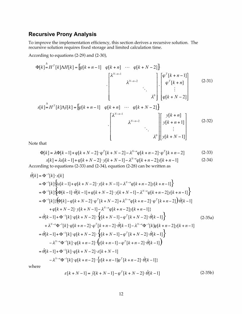
Recursive Prony Analysis To improve the implementation efficiency, this section derives a recursive solution. The recursive solution requires fixed storage and limited calculation time.

According to equations (2-29) and (2-30),

(2-31)

(2-32)

Note that

(2-33)

(2-34)

According to equations (2-33) and (2-34), equation (2-28) can be written as

(2-35a)

where (2-35b)

13

is the priori prediction noise. This priori prediction noise is the difference between the measurement at k+N-1 and the prediction based on the past ringdown model. Note that the past ringdown model is built based on the measurement taken before k+N-1 (not including k+N-1). The prediction noise serves as an indication of how well the current ringdown model describes the next available data.

Note that a recursive algorithm is formed by equations (2-33), (2-34), and (2-35), because the current estimate can be calculated by updating the previous estimate using current measurements. The storage requirements are all fixed.

Improved Recursive Prony Analysis Note that equations (2-33), (2-34) and (2-35) require the calculation of inverse matrix, , which is a time-consuming computation. The calculation efficiency improves by using matrix inversion lemma from [Ljung, 1999] given as

(2-36) to circumvent the matrix inverse calculation. To facilitate notation, define:

(2-37)

Based on this choice, equation (2-35) becomes

(2-38)

According to equation (2-37),

(2-39) Now apply the matrix inversion lemma two times.

1) Matrix inversion lemma #1

(2-40)

(2-41)

where

(2-42)

Define

(2-43) Then

(2-44)

2) Matrix inversion lemma #2

14

(2-45)

With the derivation complete, the improved recursive Prony for each time step, k, follow the following sequence:

1. use equation (2-45) to calculate Q[k],

2. use equation (2-44) to calculate P[k],

3. and use equation (2-38) to calculate .

Method for Detection of Ringdown Signals The applicability of the mode identification algorithms (including Prony analysis) rely heavily on the proper use of algorithms. Identification algorithms can provide dependable mode information only when applied properly and on the right signal types. Prony analysis is known to be applicable to ringdown data. Because of the rich modal information contained in ringdown data, the time window of the data needed for estimation is significantly shorter than that for ambient data. Thus, the latency in estimation can be reduced, and mode estimates can be updated more timely. Therefore, it is highly desirable to automate Prony analysis on identified ringdown data. Proper automatic Prony analysis relies on the detection of oscillations, and thus ringdown data. This section introduces three indices for this purpose: relative noise level, measurement energy, and prediction correction.

The relative noise level is the percentage of noise with respect to total measurement energy. It is defined as

(2-46)

where is the estimation noise from equation (2-15) and is the measurement signal of equation (2-14).

As defined in equation (2-15), the posteriori noise is the measurement component that is unexplained by the identified ringdown model. Thus, a lower relative noise level indicates a good fit between model and data, and the ringdown assumption may hold. On the other hand, a higher relative noise level indicates that the fit is not so good, and the ringdown assumption is unlikely to hold.

For the typical power system application, a sudden disturbance, such as a brake insertion, line trip, or generator trip, produces ringdown data. Ringdown data normally carries more energy than ambient data. During the period of a disturbance, the measurement energy, given by (2-47), increases. Growing signal energy may indicate the imminence of a ringdown disturbance.

15

(2-47)

Another useful metric for detecting proper algorithm application is the prediction correction, defined as

(2-48) The prediction correction is the difference between priori prediction noise, as in (2-15), and posteriori prediction noise, as in (2-35b). This describes the adjustment made after a new data point is included. A smaller prediction correction term indicates consistency between the current model and the updated model. A large prediction correction indicates significant changes in model after a new measurement data point is included. Except abrupt changes, which result in ringdown data, power system operating points slowly migrate from one to another. Thus, it is reasonable to assume that the modes do not change significantly during a ringdown procedure. Therefore, ringdown data should produce a smaller prediction correction term.

For reliably detecting ringdown data, the following method is proposed:

1) Arm the ringdown detector, when:

• the relative noise level is lower than a preselected threshold (the threshold is selected to be mean minus three standard deviations for the ambient data in this report);

• the measurement energy level exceeds a preselected threshold (the threshold is selected to be mean plus 10 standard deviations for the ambient data in this report);

• and the prediction correction is lower than a preselected threshold (the threshold is selected to be mean plus 10 standard deviations for the ambient data in this report).

2) If the ringdown detector is armed, set the start of ringdown data (i.e., the onset of oscillations) after the relative noise level reaches a local minimum point.

3) If the start of ringdown data has been set, set end of the ringdown data when the relative noise level exceeds a preselected threshold (the threshold is selected to be mean minus three standard deviations for the ambient data in this report).

Note that the recursive Prony algorithm executes continuously on all the measurement data. However, only when the ringdown data is detected utilizing the above criteria, are modes estimated from Prony analysis trusted and reported to support grid operation and other decision making. The threshold values can serve as a good rule of thumb for implementing the algorithm. They may need slight adjustment for different configurations or operating conditions of the power system to reduce the rate of false alarms and missed alarms.

16

CHAPTER 3: Results of Simulation Case Studies Simulation studies are used to evaluate the performance of the proposed recursive Prony analysis algorithm and ringdown oscillation detection method. A 17-machine model (shown in Figure 4) generates simulation data for testing the performance of the proposed method. Many studies used this model to evaluate performance of mode identification algorithms. A detailed description of the model is in [Trudnowski et al., 2006].

Figure 4: One-line Diagram of 17-Machine System

One line diagram representing the 17-machine simulation system. The 17-machine system is a very rough approximate of the western U.S. power grid. Source: [Trudnowski et al., 2006]

To conduct long-term simulations (several minutes), the 17-machine model is linearized into a linear model of order 203 using the MATLAB Power System Toolbox (PST) [Chow and Cheung, 1992]. Table 1 lists the dominant inter-area modes of this model. The mode at 0.422 Hz and 3.63% damping is selected for evaluating the performance of recursive Prony algorithm. To

17

generate the ambient data, low-pass filtered Gaussian white noise sequences simulate small real and reactive load changes at all the load buses. A half-second insertion of a 1400 MegaWatt (MW) brake at bus 35 produces ringdown data for analysis. The sampling rate of simulation data is set to be 30 samples per second to simulate PMU measurement from the WECC Wide Area Measurement System (WAMS). The sampling rate of the data set is subsequently reduced to 5 samples per second to focus on low frequency mode studies [Zhou et al., 2007].

Table 1: Inter-area Modes of 17-machine System

Freq (Hz) Damp (%) Mode Interaction

0.318 10.74 North  half vs. Southern  half

0.422 3.63 North half vs. Southern half + bus 45

0.635 3.94 bus  18 vs. Rest  of  the  system

0.673 7.63 buses  20,  21 vs. bus 24

Source: [Trudnowski et al., 2006]

To examine the statistical performance, a Monte Carlo method is used. The Monte Carlo method uses repeated random sampling to generate a group of data sets for mode estimation [Wikipedia, 2009]. It is used in the report as follows:

1) Generate M sets of random data to simulate the random load changes. In this report, M is set to be 100. Each set of data is of 120 seconds in length.

2) Apply each set of random data to the 17-machine model to simulate random load changes.

3) At the 50-second mark, apply the half-second brake insertion of 1400 MW at bus 35 to generate ringdown data. Apply the proposed ringdown detection method to detect the insertion of the brake (i.e., the start of the oscillation).

4) Apply the proposed recursive Prony analysis to identify the power system modes.

The case studies utilized the power flow on the line from bus 18 to bus 30. The objective is to see if the algorithm can accurately detect the brake insertion, and how quickly and accurately the recursive Prony analysis method can estimate the oscillation modes. A time plot of one output of the 100 Monte Carlo simulations is shown in Figure 5 (the DC component has been removed).

18

Figure 5: Single 17-Machine Simulation Output of Ambient and Ringdown Data

Single simulation output of Monte Carlo simulations using 17-machine model. Output represents both ambient and ringdown data types from the model. Source: Pacific Northwest National Laboratory

The identification parameters for the recursive Prony algorithm are set up as n=20, N=80, and λ=1. Other parameters are set as and times an appropriately sized identity matrix. Note that with selected parameters, the Prony analysis window is set to 16 seconds. Thus, the Prony analysis results begin 16 seconds after the ringdown starts. In addition, due to the 16-second time window of Prony analysis, the ringdown data needs to accumulate for 16 seconds before the proper application of Prony analysis. For this simulation study, it means that the Prony analysis should be applicable at about 50.5+16=66.5 seconds, as shown in Figure 5, where 50.5 seconds represents the time the 1400 MW brake is released from the system.

To evaluate the performance of the proposed ringdown data detection method, the three indices (relative noise level, measurement energy, and prediction correction) are calculated for each of the 100 data sets, and results are summarized in Figure 6 through Figure 8. Note that the ringdown detection method is trying to detect the proper interval to apply Prony analysis. As indicated previously, with a 16-second analysis window, this should be around 66.5 seconds.

19

Figure 6: Relative Noise Level for 100 Monte Carlo Simulations

Relative noise level for 100 Monte Carlo simulations. The red line represents the threshold of detection for which a signal would become an oscillation candidate. Source: Pacific Northwest National Laboratory

Figure 7: Measurement Energy for 100 Monte Carlo Simulations

Measurement energy for 100 Monte Carlo simulations. The red line represents the threshold of detection for which a signal would become an oscillation candidate. Source: Pacific Northwest National Laboratory

20

Figure 8: Prediction Correction for 100 Monte Carlo Simulations

Prediction correction value for 100 Monte Carlo simulations. The red line again represents the threshold of detection for which a signal becomes an oscillation candidate. Source: Pacific Northwest National Laboratory

In Figure 6, the relative noise levels behave consistently during the ringdown data for 100 sets of data. It has one peak and two valleys. The first valley is due to the over-fit on the initial large transient of the brake insertion. The second valley is where the ringdown signal detection should occur. In contrast, the relative noise levels vary significantly for ambient data. Due to the large variance of the relative noise level during the ambient data, detecting ringdown data only based on the relative noise level may result in false detection scenarios.

Figure 7 shows that the measurement energy for ringdown data is significantly larger than the ambient data portions of the simulations. Thus, it is useful for detecting ringdown data. Note that detecting ringdown data only based on the measurement energy may also result in false detection. This is due to large amplitude disturbances leading to large measurement energy.

Figure 8 shows that the prediction correction has a peak when the relative noise level in Figure 6 has the first valley. It shows that during this period, even though the relative noise level is low, mode estimation is not consistent. The adjustment after taking in a new data point is significant. Thus, it is not proper to apply Prony during this period. By combining Figure 8 with Figure 6, the first valley of the Figure 8 does not fit the ringdown data criteria.

To assist comparison, Figure 9 shows the three indices normalized and combined into one figure. The three indices show distinguishable behaviors during the ringdown data. The combination of all three indices results in a reliable method for the detection of ringdown data.

21

Figure 9: Normalized Indices for 100 Monte Carlo Simulations

Normalized indices of detection for 100 Monte Carlo simulations. All three metrics must be satisfied for an oscillation signal to be present, and for Prony analysis to be applied. Source: Pacific Northwest National Laboratory

Applying the proposed method from Chapter 2 creates Figure 10, which summarizes the identified ringdown range from the 100 data sets. On average, the ringdown detection algorithm indicates the Prony analysis should start at 66.0 seconds. That indicates the detection of ringdown data at about 50.0 seconds, on average. For 100 sets of simulation data, the standard deviation (std) of ringdown detection time is 0.7 seconds, as indicated by the thinner red dash lines. This indicates the ringdown data is detected with reasonable accuracy. In addition, on average, the ringdown data appears to end at 80.4 seconds. The standard deviation of ringdown ending time is 3.2 seconds, as indicated by the thinner blue dash lines.

22

Figure 10: Ringdown Detection Results

Ringdown detection results for 100 Monte Carlo simulations. The red line represents the average Prony starting time, with thinner red dash lines representing plus or minus one standard deviation. The blue line represents the end of the Prony interval, with thinner blue dash lines representing plus or minus one standard deviation. Source: Pacific Northwest National Laboratory

Applying the proposed Prony analysis over the detected ringdown data using a 16-second window allows the detection of the mode at 0.42 Hz. Figure 11 shows the individual 0.42 Hz modes estimated during the 100 Monte Carlo simulations. Notice that the mode estimates cluster around the true mode. It shows that even with a short 16-second window of ringdown data, the Prony analysis can provide reasonable mode estimation. In contrast, Figure 12 shows the Prony analysis results from ambient data. Observe that applying Prony analysis on ambient data with a 16-second window results in large estimation errors.

In summary, the simulation results show that the proposed method effectively detects ringdown data. Power system modes can be estimated within short time window and within relatively real-time constraints when the recursive Prony analysis is applied to the detected ringdown data.

23

Figure 11: Mode Estimates from Ringdown Data

Modal estimates obtained from applying Prony analysis on the detected oscillation interval. Blue dots represent the estimate for each of the 100 Monte Carlo trials. Source: Pacific Northwest National Laboratory

Figure 12: Modal Estimates from Ambient Data

Modal estimates obtained by applying Prony analysis to ambient data interval. Notice the high scatter of the results, indicating Prony analysis is not a good technique to apply to ambient data. Source: Pacific Northwest National Laboratory

24

CHAPTER 4: Results of Field Measurement Studies To further validate the performance, the proposed oscillation detection algorithm is applied to the field measured Phasor Measurement Unit (PMU) data. The data represent events taken from the WAMS of the WECC system. To protect the data, some data values are rescaled and the DC component is removed.

When detected, oscillations are marked over the time domain plot. In the following figures, the red dashed lines mark the first data point that is valid for Prony study. The magenta dashed lines mark the time when the Prony analysis becomes valid. Prony analysis can be performed on the data between red and magenta dash line. The distance between the red and magenta line is the Prony analysis time window. The Prony window is a constant, which is user selectable. The Prony window must be large enough so that there are enough data values for Prony equation (2-8) to have solution of reasonable accuracy. The blue dashed line marks the end of the ringdown interval. Prony analysis should be performed recursively over the data between the red and blue dashed lines.

WECC Break-up of August 10, 1996 On August 10, 1996, the western North American power grid experienced a system breakup. Later analysis revealed one of the primary causes of the system breakup to be a poorly damped inter-area oscillation around 0.25 Hz [Kosterev et al., 1999]. Figure 13 shows real power flow on the transmission line from Malin to Round Mountain just before the breakup. Figure 13 shows that a number of lines tripped producing intermediate oscillations. The proposed oscillation detection algorithm was applied to this data set to determine when the Prony analysis can be applied to generate accurate mode estimation with a relatively short time window.

As Figure 13 demonstrates, according to the algorithm, there are three oscillation instances for proper Prony analysis with a short time window. The first and last events represent line trips of the Keeler-Allston and Ross-Lexington line, respectively. Figure 14 and Figure 16 examine the detail of these two events. The middle event represents an oscillation on the system caused by device interactions. Figure 15 examines this oscillation.

Figure 14 shows a closer plot of the Keeler-Allston line trip, and the resultant oscillation. As Figure 14 indicates, Prony analysis may begin shortly after the 7.1-minute mark of the data. As shown in the data, the algorithm correctly identifies the beginning of the oscillation. The blue dashed line marks the point when the Prony analysis should stop. This line indicates where the ambient noise begins overwhelming the oscillation signal.

Figure 15 represents a visible oscillation in the original 1996 data caused by machine and control responses after the Keeler-Allston line trip. Grid dispatch and event information indicates the previously tripped Keeler-Allston line unsuccessfully reclosed shortly before this event, so it may be a major influence in the presence of this event. Examining the location of the red and blue lines, the oscillation detection algorithm appears to have successfully identified the start and end of the oscillation, which would not be visually identifiable from the raw data in Figure 15. During the identified oscillation interval, the information contained in the signal is enough to drive Prony analysis and obtain valid mode estimates.

25

Figure 13: Malin to Round Mountain Power for August 10, 1996 Event

Recorded real power flow from Malin to Round Mountain with overlaid event detail. Data is referenced from August 10, 1996 at 15:35:30 PDT. Source: Pacific Northwest National Laboratory

Figure 14: Keeler-Allston Line Trip of August 10, 1996

Detail of Keeler-Allston line trip of August 10, 1996 WECC outage. Source: Pacific Northwest National Laboratory

26

Figure 15: Second Oscillation of August 10, 1996 Event

Detail of second oscillation detected during August 10, 1996 WECC outage. Source: Pacific Northwest National Laboratory

Figure 16 shows the result of the undamped oscillations from the August 10, 1996 western interconnection breakup. The oscillation is associated with the Ross-Lexington line trip. Once again, the oscillation detection algorithm does a good job of detecting the time interval to apply Prony analysis. The beginning of the oscillation interval clearly coincides well with the time of the line tripping. During this oscillation interval, several units of the McNary Dam generation facility were tripped offline. Shortly after the oscillation in Figure 16, the western interconnection began to be unstable and separate into islands.

Figure 17 summarizes the mode analysis results for the 0.25 Hz mode using different algorithms. The blue thick line in Figure 17 shows the mode estimation results from the proposed recursive Prony study. To verify the proposed methods, the results from [Hauer 2007], using block Prony analysis and ambient data analysis, are also shown in Figure 17 as green dots. In addition, the red dashed line in Figure 17 represents the results from the application of an R3LS study of [Zhou 2007].

27

Figure 16: Ross-Lexington Event of August 10, 1996

Detail of oscillations detected for Ross-Lexington line trip of August 10, 1996 WECC Outage. Source: Pacific Northwest National Laboratory

Figure 17: Comparison of mode analysis results

Mode frequency and damping ratio estimates from three different resources. Source: Pacific Northwest National Laboratory

28

Observe that the mode estimates from the three methods are consistent, which indicates that the proposed method provides proper mode estimates. Also, observe that there are minor differences between estimation results from the different mode analysis algorithms. Note that study carried out by [Hauer 2007] is a supervised study, during which the authors’ experience chose the data and analysis methods. The R3LS of [Zhou 2009] can be executed automatically, but it needs to uses long time window (exponential window of equivalent 2-minute) because it does not distinguish between ringdown and ambient data types. In contrast, the proposed recursive Prony method automatically recognizes the ringdown responses and automatically applies a short time window for the ringdown responses. Thus, the proposed method can detect the undamped oscillation in a more timely fashion than the R3LS algorithm.

R3LS is generalized for ambient data, where long time windows help reduce the estimation variance when the modes do not change. However, when mode changes occur quickly, such as in a line tripping event, the long time window lowers the tracking capability of the algorithm. This results in large bias errors due to the averaging effect. When a ringdown oscillation appears, information density is high and the variance of mode estimation is small. Thus, a short time window, as in the proposed method, is more suitable for tracking mode changes.

In addition, mode estimates from all three methods show the decreasing frequency and damping ratio, which are an indicator of small signal stability problems. This indicates that with the on-line Prony analysis capability, one would be able to issue early warning of the small signal stability problem before the system breakup on August 10, 1996.

Brake Insertion of November 14, 2002 Ringdown oscillations in the power grid are often associated with lines and generators switching or tripping offline. Another source of oscillations on the power system is the deliberate excitation via a large shunt resistance. Figure 18 and Figure 19 show the results of inserting a large 1400 MW resistance into the western power system. This 1400 MW resistor, referred to as the Chief Joseph Dynamic Brake, is often switched in momentarily either to aid in improving the stability of the system during machine acceleration events, or to deliberately excite the power system for testing the dynamic response of the system.

Figure 18 shows an overall view of an insertion of the Chief Joseph Dynamic Brake on November 14, 2002. As the figure demonstrates, the detection algorithm detects the oscillation interval. Unlike the August 10, 1996 case presented previously, the oscillation event is very prominent and easy to spot visually from the raw data. Figure 19 shows a closer view of the brake insertion and the detected oscillation interval using the oscillation detection algorithm.

29

Figure 18: Brake Insertion of November 14, 2002

Line flow measurement on WECC system for November 14, 2002. System event represents insertion of the Chief Joseph Dynamic Brake into the system. Source: Pacific Northwest National Laboratory

Figure 19: Brake Insertion of November 14, 2002 Detail

Detail of line flow measurement on WECC system for November 14, 2002. System event represents insertion of the Chief Joseph Dynamic Brake into the system. Source: Pacific Northwest National Laboratory

30

As Figure 19 demonstrates, the algorithm detects the start of the oscillation interval very well. An application of Prony analysis from this point would yield a good estimate of the ringdown modal content. In addition, the detection algorithm indicates that Prony analysis can continue until approximately the 201-second mark. The final Prony analysis should encompass the interval between roughly 170 seconds to 201 seconds. There are clearly still significant components to the resultant ringdown at this point in the data, so the oscillation algorithm is still successfully detecting a valid Prony analysis range.

Alberta Separation of June 10, 2002 As indicated earlier, one of the routine causes of an oscillatory event on the power system is a transmission line switching or tripping event. Figure 20 shows the measurement data for such an event. On June 10, 2002, the Alberta, Canada power grid separated from the rest of the WECC grid. As shown in Figure 20, an oscillation occurred when the system moved towards a new equilibrium point.

Figure 20: Alberta Separation of June 10, 2002

Line flow measurement on WECC system for June 10, 2002. System event represents a separation of Alberta, Canada from the rest of the WECC system. Source: Pacific Northwest National Laboratory

Figure 20 shows the data of the June 10, 2002 Alberta separation event. This event is not very prominent visually in the data interval presented. Without prior knowledge of the event or the oscillation detection algorithm, it is easy to overlook this event. Figure 21 shows a closer view of the event and the oscillation detection algorithm results.

31

Figure 21: Detail of June 20, 2002 Alberta Separation

Detail of line flow measurement on WECC system for June 10, 2002. System event represents a separation of Alberta, Canada from the rest of the WECC system. Source: Pacific Northwest National Laboratory

Upon closer inspection, there is clearly an oscillatory event associated with the Alberta separation. As Figure 21 shows, the oscillation detection algorithm selects a reasonable interval for valid Prony analysis. The beginning of the selected interval is a valid starting point for Prony analysis and the oscillation-ending interval is reasonable, given the data.

Palo Verde Generation Trip of November 18, 2000 Generator tripping events are also a prominent cause of oscillatory events on the power system. On November 18, 2000, a loss of generation occurred at the Palo Verde generation facility. Figure 22 shows the measurement data for this loss of generation.

As with the previous figures, Figure 22 overlays the results of the oscillation detection algorithm. With a large response to the loss of the generation, the oscillation detection algorithm had little trouble locating the proper interval to begin Prony analysis. The oscillation detection algorithm indicated Prony analysis would remain valid until the interval ending around 95 seconds. If the oscillation start time is offset by the 35-second Prony interval, significant components of the generation trip’s oscillation are still present in the analysis interval, indicating the validity of Prony over that interval.

32

Figure 22: Palo Verde Generation Trip of November 18, 2000

Line flow measurement on WECC system for November 18, 2000. System event represents a trip of generation units at the Palo Verde facility. Source: Pacific Northwest National Laboratory

PDCI Block on November 2, 2004 Different forms of oscillations are also possible from normal transmission lines tripping, or other disturbances on the power system. Figure 23 shows the high voltage, long DC line switching event that occurred on November 2, 2004. During this event, a planned adjustment on the Pacific DC Intertie resulted in a readjustment of the amount of power that the parallel AC lines were carrying.

A closer examination of the oscillation appears in Figure 24. As with some of the previous examples, the event is prominent when compared to the surrounding data. However, without explicit knowledge of when the event occurred, and without the use of the oscillation detection algorithm, this event could easily be missed during normal grid operations.

Figure 24 shows the algorithm clearly detects the ringdown associated with the PDCI event. It appears the oscillation analysis begins a cycle too late. However, the significantly larger swings of the first cycle of the oscillation are not at the same frequency as the rest of the ringdown due to non-linear behaviors. Therefore, the detection algorithm does not consider this a valid oscillation for the ringdown analysis. An examination of the prediction correction factor would likely show a large deviation as the oscillation moves to a different frequency. As with other detections, once the ringdown event begins to have amplitudes similar to ambient data, the algorithm indicates the Prony analysis interval is complete.

33

Figure 23: PDCI Block of November 2, 2004

Line flow measurement on WECC system for November 2, 2002. System event represents a planned adjustment of the Pacific DC Intertie that resulted in effects elsewhere on the system. Source: Pacific Northwest National Laboratory

Figure 24: Detail of PDCI Block of November 2, 2004

Detail of line flow measurement on WECC system for November 2, 2002. System event represents a planned adjustment of the Pacific DC Intertie that resulted in effects elsewhere on the system. Source: Pacific Northwest National Laboratory

34

Alberta Separation of July 24, 2006 An earlier example examined an event caused by the separation of Alberta, Canada from the rest of the WECC. Figure 25 represents another Alberta separation on July 24, 2006. Unlike the previous example, the separation is barely visible in Figure 25. The large, initial oscillation in Figure 25 is predominantly a dynamic brake insertion following the faulting of another line in the WECC system. This Alberta separation further differs from the earlier example in that a secondary event later in the data is present.

Figure 25: Alberta Separation of July 24, 2006

Line flow measurement on WECC system for July 24, 2006. System events represent the separation of Alberta, Canada from the WECC system, followed by a secondary event. Source: Pacific Northwest National Laboratory

Figure 25 shows the overall oscillation detection algorithm results for the Alberta separation event. As the figure indicates, there are actually three oscillations detected over the data interval. Figure 26 shows the first event in detail. The second and third events appear in Figure 27.

35

Figure 26: Brake Insertion of July 24, 2006 Alberta Separation

Detail of line flow measurement on WECC system for July 24, 2006. System event represents the separation of Alberta, Canada from the WECC system, with a corresponding insertion of the Chief Joseph Dynamic Brake. Source: Pacific Northwest National Laboratory

The first event of the Alberta separation data set represents a line fault and the insertion of the Chief Joseph Dynamic Brake. The actual Alberta separation occurs around the 810-second mark and is not prominent on the data. Therefore, it was not flagged as a valid Prony interval by the oscillation detection algorithm. Recall that the purpose of the proposed oscillation detection algorithm is to identify proper ringdown oscillation data for the proper application of Prony analysis. Because of low SNR, the data from the non-prominent oscillation is not suitable for Prony analysis.

Figure 26 shows the oscillation that resulted from a brief Chief Joseph brake insertion. The oscillation detection algorithm successfully detects the start of a suitable Prony analysis interval. The analysis interval appears to extend well beyond the ringdown data. However, closer examination of Figure 26 reveals a secondary oscillation event over the 850 and 880-second time interval. Given the larger amplitude of the initial oscillation, the secondary oscillation could easily have been present, but not apparent in the signal at that time.

Along with the primary, line-trip event association with the Alberta separation, a secondary series of events were also observed. Figure 27 shows the oscillatory events caused by a generation trip, and later responses to that tripping event. The algorithm successfully detects the oscillation at the 1505-second mark. This oscillation resulted from the trip of a generator at the Colstrip generation facility. Approximately a minute later, other smaller events occurred on the system. While the cause of these oscillations is uncertain at this time, shunt capacitor bank switches are likely candidates. Despite not being as prominent as the initial generator trip

36

event, Figure 27 shows these events were clearly oscillatory in nature and successfully detected by the algorithm.

Figure 27: Colstrip Generation Trip of July 24, 2006 Alberta Separation

Detail of line flow measurement on WECC system for July 24, 2006. System events represent the trip of a Colstrip generation unit and a secondary event following the separation of Alberta, Canada from the WECC system. Source: Pacific Northwest National Laboratory

California Machine Control Event of January 4, 2010 As indicated earlier in the examples, line trip events and system separations are not the sole cause of oscillatory behavior on the system. Generator controls can also produce oscillatory responses on the system. Figure 28 shows an oscillation caused by a California generator on January 4, 2010. As Figure 28 and the detail plot in Figure 29 show, the event is very prominent, but does not begin with an abrupt shift like most of the other oscillation examples presented.

As Figure 28 shows, the generation oscillation event is visually prominent on the measured data. Unlike the line tripping and system separation events, there is no discrete cause of the oscillation. Rather, the oscillation amplitude slowly increases in response to the event. Despite the lack of a discrete oscillation start, the oscillation detection algorithm still locates suitable starting and ending times for ringdown analysis of the event. Figure 29 provides a detailed plot of the oscillation detection times.

37

Figure 28: California Machine Event of January 4, 2010

Line flow measurement on WECC system for January 4, 2010. System event induced by a control event in a generation plant in California. Source: Pacific Northwest National Laboratory

Figure 29: Detail of California Machine Event of January 4, 2010

Detail of line flow measurement on WECC system for January 4, 2010. System event induced by a control event in a generation plant in California. Source: Pacific Northwest National Laboratory

38

The oscillation is very prevalent in the detail plot of Figure 29. Despite the higher frequency of the oscillation produced by this event, the detection algorithm produces a valid Prony analysis interval. Examination of the plot indicates the oscillation may have started a few seconds before the red oscillation start line the algorithm determined. However, at this point in the data, the oscillation is still at approximately the same amplitude as the ambient power system noise. This smaller amplitude and less consistent nature of the oscillation required a couple of seconds more data before the detection algorithm indicates a valid interval. Despite this possibly delayed starting interval, the ringdown stop interval appears very well selected with the end of the ringdown associated with the event.

Figure 28 and Figure 29 represent the application of the ringdown detection algorithm over a short data interval. For a practical dispatch center application, the ringdown oscillation detector would be running over the full 24 hours of the day. To evaluate this performance, the ringdown oscillation detection algorithm was run on the full January 4, 2010 data set. According to dispatch records, the California machine control event was the only disturbance recorded over the 24-hour period. The ring-down detection algorithm only detects one event over the 24-hour interval as well. Furthermore, some measurement errors were present in the data. The ringdown oscillation detection algorithm successfully ignores these non-typical data points and does not register a false alarm. Figure 30 shows the detail of the detection.

Figure 30: Detail of 24-hour Oscillation Detection Run

Detail of line flow measurement on WECC system for January 4, 2010. System event induced by a control event in a generation plant in California. Results obtained from 24-hour recursive run of oscillation detection algorithm. Source: Pacific Northwest National Laboratory

39

As Figure 30 shows, the ringdown oscillation detection algorithm still detects the California machine control event, despite having been running for approximately 17 hours already. As the figure shows, the detected analysis interval is slightly different than that of Figure 29. This is primarily a result of the longer data set. After running for 18 hours, the detection algorithm has a different estimate of the relative noise of the system. As such, the increasing amplitude of the oscillation takes more time to resolve than the shorter data set case. This also explains the shorter Prony interval compared to Figure 29, as shown by the blue dashed-line appearing earlier. Despite these differences, the algorithm still detected a sufficient interval to apply the Prony analysis method.

40

CHAPTER 5: Implementation and User Interface Design With the basic algorithm developed, it needed to be implemented for testing on simulated and measured power system data. The algorithm was fully implemented using the Mathworks MATLAB software. As a result, MATLAB became the basis for implementing the algorithm for testing, as well the basic platform for a graphical user interface (GUI).

The MATLAB environment produced the results presented in Chapters 3 and 4. The 17-machine model was used to generate simulation data, which resulted in settings for the three ringdown detection criteria described in Chapter 3. Chapter 4 utilized field measurement PMU data from the western United States power grid, extracted into MATLAB, to validate the proposed method.

To provide a user-friendly interface, the oscillation detection and analysis method was integrated into an existing MATLAB GUI for ModeMeter at the Pacific Northwest National Laboratory. The oscillation detection and analysis method supplements the functionality of the ModeMeter GUI. The GUI intends to significantly improve the usability of the method and facilitate the adoption of the method in the grid operation environment. Figure 31 shows a sample screen of the ModeMeter GUI. The GUI allows the oscillation detection and analysis method to directly access the field measurement data in PSMT format, which is a standard data format for PMU data supported by Dynamic System Identification toolbox [NASPI, 2010a; NASPI, 2010b].

Figure 31: Sample Output of the MATLAB-based GUI

MATLAB GUI running the August 10, 1996 blackout data. Note that an oscillation is being detected, which represents the secondary oscillation presented in the earlier section. Source: Pacific Northwest National Laboratory

The MATLAB GUI is fully functional and is ready for pilot testing in control rooms. One advantage of the MATLAB GUI is that it is easy to maintain and update for prototype algorithm

41

development. However, it requires a MATLAB license, instead of being a standalone tool. To further improve the portability and applicability of the GUI, this project explored implementing the algorithm with C++ language. Figure 32 shows the proposed design of the C++-based GUI. Compared with Figure 31, it is apparent the C++ GUI is attempting to mirror the functionality of the MATLAB-based GUI.

Figure 32: Concept for C++-based GUI

Initial concept screen for C++-based oscillation detection GUI. Circles represent areas of functionality described in this section. Source: Pacific Northwest National Laboratory

The proposed graphical user interface of the C++ ModeMeter consists of four major functional areas, each circled in Figure 32. The highlighted areas represent the following implementation guidelines:

1. Data Entry – Data originates from two sources: a real-time data stream, or an offline .csv data file. As such, a clear method for selecting the desired input is necessary. For the first one, phasor data concentrator (PDC) communication protocols retrieve data from a real-time stream. For the latter one, a .csv file is located on the computer through the “Load” button on the GUI. This allows the data to be loaded from an offline source, and then simulate the real-time processes of the GUI.

2. Sequence Control - “Play,” “Stop,” and “Close” buttons control the data update process of the oscillation detection GUI when using an offline data source. If utilizing offline, saved data sets, it may useful to run the algorithm in faster than real-time. The “Speed” trackbar controls the update speed of the data source. For example, if “8” is specified, the data is imported at rate 8x that of the original display time.

3. Data Display - Data Display is composed of plotting displays and tabular array display. These plots provide the user feedback on the algorithm modal analysis and oscillation detection. There are four plotting panels on the ModeMeter GUI, which perform a variety of tasks and draw different dynamic curves or plots upon received new data.

42

The Major Modes tabular table shows the parameters of modes of interest, dynamically based on the results of the oscillation detection algorithm.

4. Time Display - Time Display shows both the program’s overall running time, and the elapsed plotting time based on a particular source of data.

Part of the future work would be to continue the development of the C++-based GUI towards a tool for control room use. At the conclusion of this project, initial layouts and displays for the C++ GUI are set and working. Furthermore, the following two tasks have been identified to get the C++-based GUI ready as a standalone tool. First, a suitable package of matrix-capable solvers must be selected and integrated. This requirement allows the implementation of the ringdown analysis algorithm. The initial code exists, but requires a resolution of this missing capability and in turn requires further work to implement the solvers. Secondly, the C++ GUI needs testing and refinement using field measurement PMU data. Once the above two tasks are finished, prototype C++ GUI tool will be available for more extensive testing and eliminate the requirement of MATLAB license.

43

CHAPTER 6: Conclusions and Future Work Conclusions This project developed, implemented, and evaluated a recursive Prony algorithm for automatically detecting and analyzing power grid oscillations in near real time using PMU data.

Modal analysis provides vital information about the power system stability. On-line mode identification algorithms based on PMU measurements provide a way for monitoring power system modes in near real time. Oscillation alarms can be issued when the power system is lightly damped. A good oscillation alarm tool (a.k.a. ModeMeter) can provide time for operators to take remedial reaction and reduce the probability of a system breakup from such a light damping condition.

The applicability of the mode identification algorithms relies heavily on the proper use of algorithms. Identification algorithms can provide dependable mode information only when applied properly on the right signal types. Improper application of algorithms, such as applying Prony’s method to ambient data, may result in false alarms and/or missing alarms.

One of most important categories of data is the oscillation ringdown data, which results from major disturbances. It is important to detect the oscillation ringdown for proper application of Prony’s method. The proper application allows the identification of modes within a short time window.

In this report, a method for detecting ringdown data is proposed and evaluated. Through Monte Carlo simulation, it was shown that Prony analysis can be applied automatically and properly on the detected ringdown data to estimate the power system modes. The evaluation based on the field measurement shows that the proposed method is applicable to the measurement data and produces the expected results. By effectively identifying ringdown data, the modes can be identified accurately within a short time window. Thus, the detection reduces the rate of false and missing alarms.

A MATLAB-based GUI provides a user-friendly interface for using the algorithm, and for further validity testing. With the ability to utilize offline data or incoming PMU streams, the MATLAB GUI provides interested parties with the flexibility to investigate and evaluate the ringdown algorithm’s performance. Initial efforts were put forth to migrate the GUI to a more generic C++ platform to eliminate the needs for MATLAB licenses. The initial interface C++ has been established and tested. In addition, some additional coding efforts are identified to resolve some matrix computation issues necessary to build a fully functional, and more portable, C++ GUI.

44

Impact and Future Work By providing accurate and timely information about the oscillation modes of power grid, the study results from this project can help lower the probability of large-scale blackouts, and increase the power grid efficiency. Unstable oscillations can cause power grid breakups and even large-scale power outages, such as the power outage that occurred on August 10, 1996 in the western interconnection. During the outage in 1996, about 7.5 million customers (24 million people) lost their power supply for the range from several minutes to 6 hours [Wikipedia contributors, 2010]. According to Table 6-1 of the proposal for the Western Interconnection Synchrophasor Program (WISP) [WECC, 2009], the value of large-scale outage avoidance for the WECC system is over one billion dollars over the next 40 years. According to [Western Congestion et al., 2006], most major tie lines in WECC system are often constrained by stability limits, which are more limiting than the thermal limits. The early warnings for unstable modes allow the grid to operate at its full capacity, while staying within the stability boundary. The method developed in this project is expected to have significant impact on power grid operation, as it will improve reliability and avoid significant economic losses. This oscillation study is a major breakthrough in the sense that it significantly lowers false and missing alarms, as well as shortens detection time by applying oscillation detection and analysis algorithms properly.

However, the study is also limited in the sense of real world applications, and requires additional efforts to realize the full benefit. First, the method is only tested with a small, simplified model and limited number of field measurement cases. Even though the initial testing shows promising results, it needs further studies to guarantee sufficient robustness and reliability under typical operating conditions. Such a requirement is necessary for a useful control room tool. Thus, future work includes extensive testing studies with large amount of field measurement data. Revisions and improvements shall occur on the algorithm as a result of this testing.

Second, the project only focuses on the detection and analysis of oscillations. With the oscillation information available, a natural next step is to produce actionable information to increase damping, effectively suppressing the oscillations. Once the two proposed studies are complete, the benefit of oscillation study can be fully realized through improved reliability and efficiency of power grid operation.

45

References Chow, J.H., and K. W. Cheung, “A toolbox for power system dynamics and control engineering

education and research,” IEEE Transactions on Power Systems, vol.7, no.4, pp.1559-1564, November 1992.

Hauer, J.F., C. J. Demeure, and L. L. Scharf, “Initial Results in Prony Analysis of Power System Response Signals,” IEEE Transactions on Power Systems, vol. 5, no. 1, pp. 80-89, February 1990.

Hauer, J. F., W. A. Mittelstadt, K. E. Martin, J. W. Burns, and H. Lee in association with the Disturbance Monitoring Work Group of the Western Electricity Coordinating Council, “Integrated Dynamic Information for the Western Power System: WAMS Analysis in 2005,” Chapter 14 in the Power System Stability and Control volume of The Electric Power Engineering Handbook, edition 2, L. L. Grigsby ed., CRC Press, Boca Raton, FL, 2007.

Kamwa, I., G. Trudel, and L. Gerin-Lajoie, "Low-order Black-box Models for Control System Design in Large Power Systems," IEEE Transactions on Power Systems, vol. 11, no. 1, pp. 303-311. February 1996.

Kosterev, D. N., C. W. Taylor, and W. A. Mittelstadt, “Model Validation for the August 10, 1996 WSCC System Outage,” IEEE Transactions on Power Systems, vol. 14, no. 3, pp. 967-979, August 1999.

Liu G., and V. Venkatasubramanian, "Oscillation monitoring from ambient PMU measurements by Frequency Domain Decomposition," Proceedings of the IEEE International Symposium on Circuits and Systems, Seattle, WA, May 2008, pp. 2821-2824.

Ljung, L., System Identification: Theory for the User, 2nd edition, Prentice Hall, Upper Saddle River, New Jersey, 1999.

Messina, A. and V. Vittal, “Nonlinear, non-stationary analysis of interarea oscillations via Hilbert spectral analysis,” IEEE Transactions on Power Systems, vol. 21, no 3, pp. 1234-1241, August 2006.

NASPI contributors (August 2010), Dynamic System Identification Toolbox Details. Accessed August 20, 2010. [Online]. Available: http://www.naspi.org/toolRepository/tool_details.aspx?tid=54.

NASPI contributors (August 2010), Dynamic System Identification Toolbox download. Accessed August 20, 2010. [Online]. Available: http://www.naspi.org/resources/pitt/DSITools_20070802SentOutStripDownCompiled.zip.

Pal, B. and B. Chaudhuri, Robust Control in Power Systems, Springer US, 2005.

Pierre, J.W., D.J. Trudnowski, and M. K. Donnelly , “Initial results in electromechanical mode identification from ambient data,” IEEE Transactions on Power Systems, vol.12, no.3, pp. 1245-1251, August 1997.

Pierre, J. and N. Zhou, "R3LS with Finite Duration Exponential Window," worknotes, Dec. 2007.

Sanchez-Gasca, J. J., and J. H. Chow, “Performance Comparison of Three Identification Methods for the Analysis of Electromechanical Oscillations”, IEEE Transactions on Power Systems, vol. 14, no. 3, pp. 995-1001. August 1999.

46

Trudnowski, D., M. Donnelly, and E. Lightner, “Power-System Frequency and Stability Control using Decentralized Intelligent Loads,” Proceedings of the 2005/2006 IEEE PES T&D Conference and Exposition, Dallas, TX, pp. 1453-1459, May 2006.

Trudnowski, D., J. Pierre, N. Zhou, J. Hauer, and M. Parashar, “Performance of Three Mode-Meter Block-Processing Algorithms for Automated Dynamic Stability Assessment,” IEEE Transactions on Power Systems, vol. 23, no. 2, pp. 680-690, May 2008.

Western Congestion Analysis Task Force, "Western Interconnection 2006 Congestion Assessment Study," May 2006.

Western Electricity Coordinating Council, “The Western Interconnection Synchrophasor Project,” August 6, 2009

Wikipedia contributors. (November 2009) Monte Carlo method. Accessed November 23, 2009. [Online]. Available: http://en.wikipedia.org/wiki/Monte_Carlo_method.

Wikipedia contributors. (August 2010) 1996 Western North-America summer blackouts. Accessed August 20, 2010. [Online]. Available: http://en.wikipedia.org/wiki/1996_Western_North-America_summer_blackouts

Zhou, N., J. Pierre, and J. Hauer, “Initial Results in Power System Identification from Injected Probing Signals Using a Subspace Method,” IEEE Transaction on Power Systems, vol. 21, no. 3, pp. 1296-1302, August 2006.

Zhou, N., J. Pierre, D. Trudnowski, and R. Guttromson, “Robust RLS Methods for On-line Estimation of Power System Electromechanical Modes,” IEEE Transactions on Power Systems, vol. 22, no. 3, Aug. 2007, pp. 1240-1249, August 2007.

Zhou, N., D. Trudnowski, J. Pierre, and W. Mittelstadt, “Electromechanical Mode On-Line Estimation using Regularized Robust RLS Methods”, IEEE Transactions on Power Systems, vol. 24, no. 4, pp. 1670-1680, November 2008.

Zhou, N., D. Trudnowski, and J. Pierre, “Mode Initialization for On-Line Estimation of Power System Electromechanical Modes,” Proceedings of the 2009 Power Systems Conference and Exposition (PSCE), Seattle, WA, March 15-19, 2009.