ortmann, regina / pummerer, erich - uni-paderborn.de
TRANSCRIPT
No. 15 / September 2015 Ortmann, Regina / Pummerer, Erich Formula Apportionment or Separate Accounting? Tax-Induced Distortions of Multinationals’ Locational Investment Decisions

Acknowledgments
We would like to thank Tobias Bornemann, Eva Eberhartinger, Fabian Failenschmid, Thomas Hoppe, Lillian Mills, Richard Sansing, Caren Sureth-Sloane, the participants of the Poster Session of the ATA Midyear Meeting 2015 in Washington DC, the members of the DIBT Doctoral Program in International Business Taxation at Vienna University of Economics and Business, the participants of the CETAR Young Researcher Seminar at the University of Paderborn and the participants of the Research Workshop of the Faculty of Economics and Business (University of Paderborn) in Bad Arolsen 2015 for their helpful comments. Any remaining errors or inaccuracies are, of course, our own. Financial support from the Austrian Science Fund (FWF grant W 1235-G16) is gratefully acknowledged.
Formula Apportionment or Separate Accounting? Tax-Induced Distortions of
Multinationals' Locational Investment Decisions
Regina Ortmann, University of Paderborn and Vienna University of Economics and Business
Erich Pummerer, University of Innsbruck
Abstract
We examine which tax allocation system leads to more severe distortions with respect to locational
investment decisions. We consider separate accounting (SA) and formula apportionment (FA). The
effects of both systems have been hotly debated in Europe in the past years. The reason is that the EU
Member States are striving to implement a common European tax system that would lead to a switch
from SA to FA. While existing studies focus primarily on the impact of taxes on locational decisions
under either SA or FA, the main innovation of this paper is that it compares both systems with regard
to the level of distortions they induce. We compare the optimal pre-tax investment decision with the
optimal after-tax investment decision and infer from the difference in the allocation of investment
funds which tax allocation system causes more severe distortions. We assume that the multinational
group (MNG) has comprehensive book income shifting opportunities under SA. We find that the
investment incentives under SA are opposed to those under FA for a profitable investment project.
Whereas under SA as much as possible should be invested in a high-tax country, under FA as much as
possible should be invested in a low-tax country. The distortions of locational investment decisions
tend to be more severe under SA than under FA if a greater share of investment funds is to be invested
in a low-tax country from a pre-tax perspective and the investment is profitable. Vice versa, locational
decisions may be more distorted under FA if the optimal pre-tax investment decision requires
investing a major share of funds in the high-tax country. In contrast to the often stated insensitivity of
FA towards income shifting, we find the introduction of a tax allocation system based on FA in
Europe could lead to a severe shift of economic substance to low-tax countries. The results of this
paper are of particular interest for European policy makers and MNGs as our findings may induce
European MNGs to reassess their recent locational investment decisions in the face of a potential
future change in the applied tax allocation system.

1
1. Introduction
The aim of this paper is to examine which tax allocation system for multinational groups (MNGs)
causes more severe distortions of locational investment decisions. We consider two systems, namely
separate accounting (SA) and formula apportionment (FA). As both are based on a fundamentally
different mechanism for determining the tax base per entity, they offer different incentives with
respect to the favorable country of investment. We use the optimal investment decision from a pre-tax
perspective as a benchmark to assess the level of distortion caused by taxation. Thus, taking a business
perspective, we compare the optimal pre-tax investment decision with the optimal after-tax investment
decision and infer from the difference in the allocation of investment funds which tax allocation
system causes more severe distortions. Assuming comprehensive income shifting possibilities under
SA, we find that the investment incentives under SA are opposed to those under FA for a profitable
investment project. Whereas under SA as much as possible should be invested in a high-tax country,
under FA as much as possible should be invested in a low-tax country. Furthermore, locational
investment decisions tend to be distorted more severely under SA if the largest share of investment
funds is invested in the low-tax country from a pre-tax perspective. Vice versa, locational decisions
may be more distorted under FA if the optimal pre-tax investment decision requires investing a major
share of funds in the high-tax country. In contrast to the often stated insensitivity of FA towards
income shifting, we find the introduction of a tax allocation system based on FA in Europe could lead
to a severe shift of economic substance to low-tax countries.
The effects of both tax allocation systems have been hotly debated in Europe in the past years,1 the
reason being that the EU Member States are striving to implement a common European tax system. If
this should come to pass, the traditional system of SA used currently across the EU will be replaced by
FA. The idea behind the Common Consolidated Corporate Tax Base (CCCTB) system is to harmonize
EU Member States’ tax bases in order to reduce the economic hurdles resulting from 28 different
national tax systems. In 2011, the European Commission proposed a Council Directive on a CCCTB.2
If the CCCTB is introduced, European MNGs would need to apply only one tax code to determine
their tax base. The profits and losses of all single entities could be consolidated on the group level. The
consolidated group tax base would subsequently be allocated to each entity according to an
apportionment formula based on assets, labor, and sales.
In a globalizing world, companies increasingly establish a multinational company structure to remain
competitive and build more permanent establishments and subsidiaries abroad.3 By doing so, they
hope to, e.g., tap into new markets, relocate production closer to the required natural resources, or to
access lower-wage labor. Furthermore, MNGs attempt to create a tax-favorable group structure so they
1 For an overview of the historical development of the idea to harmonize the tax systems in Europe see Dahle (2011), pp.
107-109. 2 See European Commission (2011). 3 See Devereux & Maffini (2006), p. 1.
2
can benefit from tax rate differentials between countries. There is plenty of empirical evidence4 to
indicate that MNGs shift income from high-tax to low-tax countries. They do so largely via two
channels. Either MNGs shift accounting profits, meanings they merely move book values.
Alternatively, they shift real economic substance, e.g., workforce and assets, to generate profits or
losses in tax-favorable environments. Thus, real activity shifting certainly affects the structure of an
MNG. In this study we focus on locational decisions relating to real investments as a specific form of
real activity shifting. Whereas previous studies mainly identify the direction of activity shifting under
either tax allocation system separately, we go one step further and determine the level of activity
shifting under either tax allocation system and subsequently compare their respective distortive power.
The fiscal environment is currently undergoing vast changes. In the context of its Base Erosion and
Profit Shifting (BEPS) project, the OECD stated that “[t]axation is at the core of countries'
sovereignty, but in recent years, multinational companies have avoided taxation in their home
countries by pushing activities abroad to low or no tax jurisdictions.”5 This statement stresses that
fiscal authorities are increasingly concerned about how to ensure that MNGs pay their fair share of
taxes in the respective countries. Accordingly, the aim of the BEPS project is to change fiscal
framework conditions on an international level in such a way that income shifting is prevented. There
are two major tax allocation systems according to which the taxable share of each group entity is
determined: SA and FA. SA is currently used in Europe and in most countries around the world.
Under SA, each group entity that is incorporated in one country is treated distinctly and has to
calculate its tax liability separately according to national tax laws. Under FA, the uniformly
determined profits and losses of the entities are consolidated on the group level and are subsequently
allocated to the group entities according to a specific apportionment formula. This formula is designed
to capture the economic share contributed by each entity to the MNG’s profits. FA is already well-
known as it is in use, e.g., on the state level in the USA and Canada for cross-state or -province tax
base allocation. Empirical and analytical studies show that activity shifting is conducted under both
systems.6 However, to our knowledge there is no study that compares the distortive impact of either
system on locational investment decisions. As both tax allocation systems apply different mechanisms
to determine the taxable share per country, they each offer varying leeway for avoiding taxes with
respect to activity and accounting profit shifting.
From a macroeconomic perspective, a basic prerequisite for a good tax system is efficiency. Economic
entities ought to be taxed in such a way that the scarce resources of an economy are allocated in a
welfare-enhancing manner. Generally, free competition between economic entities is considered the
market type that leads to such welfare-enhancing allocation. Thus, the tax system ought to be designed
in such a way that it does not affect free market conditions. Consequently, economic entities’
4 See section 2, literature review. 5 See OECD (2013), p. 9. 6 See Martini et al. (2013), Altshuler & Grubert (2010).

3
decisions should not be affected and investment decisions should not be distorted by corporate
taxation.7 In this study we investigate to what extent SA and FA are capable of ensuring such
neutrality with respect to locational investment decisions.
We develop an analytical model to resolve our research question, namely which tax allocation system
causes more severe distortions to locational investment decisions. The MNG has to decide which share
of total investment funds to invest in each entity. We take a two-step approach, first determining the
optimal after-tax allocation of investment funds under both tax allocation systems. The optimal after-
tax allocation of investment funds is characterized by the highest after-tax cash flows under each
system. Second, to determine the level of distortion caused by each system, we calculate the difference
between the optimal allocations of investment funds from a pre-tax and an after-tax perspective. By
comparing these differences we can derive conclusions about the distortive power of each system – the
greater the difference, the greater the distortive power. The optimal economic pre-tax investment
decision is determined by the relative demand per country, as the MNG will aim to produce wherever
its sales are incurred. The optimal after-tax investment decision is modeled explicitly in our analysis.
In our model the MNG faces a trade-off between choosing a tax-optimal allocation of investment
funds and an optimal allocation from a purely economic pre-tax perspective.
We chose a two-country, two-entity setting for an MNG and assume a tax rate differential between
both countries. Under SA, we assume that book income can be shifted comprehensively due to
favorable transfer pricing arrangements. The shifting possibilities allow for the geographic segregation
of sales and expenses, which directly affects the locational investment decision. We are convinced that
it is also possible to shift book income under FA8 but do not believe that this has a direct impact on the
locational investment decision. As under FA the allocation of profits is based on the location of real
economic factors, it ought to be an MNG’s first priority to locate the economic factors in a tax-optimal
way.
The results of this paper are of particular interest for European policy makers. On an aggregated level,
our results make it possible to anticipate the macroeconomic effects induced by the potential
introduction of the CCCTB system. Furthermore, our results can benefit European MNGs that face
locational investment decisions. As we take a business perspective, our results may induce European
MNGs to reassess their recent locational investment decisions in the face of a potential future change
in the applied tax allocation system. Although our analysis is mainly motivated by the European
debate around introducing the CCCTB, the results are also interesting for policymakers and MNGs in
other parts of the world. On the state level in the US FA and SA coexist. As a matter of principle, the
states apply formula apportionment. However, “if the allocation and apportionment provisions […] do
7 See Kruschwitz et al. (2003), p. 328. 8 See Kiesewetter et al. (2014).
4
not fairly represent the extent of the taxpayer’s business activity in this state”9 US based companies
may also apply separate accounting. Prior US studies on FA10 have examined its distortive effects yet
we are the first to compare the level of distortion induced by FA relative to that induced by SA. Thus,
our results may offer new input for potential reform debates about the coexistence of both systems in
the US.
The next section consists of a brief review of the related literature. Section 3 presents the assumptions
and the model set-up. In Section 4 we examine which tax allocation system offers stronger incentives
to make an optimal locational investment decision, on the assumption that no costs are incurred by
production and sales being in different countries. In Section 5 we introduce costs for production and
sales being in different countries and determine the conditions under which either tax allocation
system more severely distorts the investment decision. We conclude with a discussion of the
managerial and tax policy implications.
2. Literature Review
Two main streams of research are relevant to our research question. First, prior research examines the
impact of taxation on the location of profits and of investment decisions. Many empirical studies
investigate how tax rate differences between countries affect the location of profits of MNGs. All of
these studies are conducted in an SA setting. We, too, examine the relationship between the location of
profits and tax rate differentials. However, doing so reflects our research question only on an
aggregated level since we go one step further and examine the underlying locational investment
decisions that determine the location of profits.
Harris et al. (1993) examine the level of tax payments of US parent companies depending on the
location of their subsidiaries. They find evidence that groups with subsidiaries in low-tax countries
pay relatively fewer taxes in the US compared to those that have subsidiaries in high-tax countries.
They conclude that US MNGs are likely to shift income. In line with that finding, Bartelsman and
Beetsma (2003) find evidence for income shifting in 16 OECD countries as well. They estimate that at
the margin 65% of additional revenues from a unilateral tax increase is lost due to a decrease in the
reported tax base. By contrast, the more recent income shifting literature identifies fundamentally
smaller shifting effects in response to changes in tax differentials. In a meta-analysis Heckemeyer and
Overesch (2013) review empirical studies on profit shifting and find that overall, reported profits
decrease by about 0.8% for each one percentage point increase in the tax differential between
countries. Dischinger et al. (2014) focus on the role of the location of the headquarters of MNG that
shift income. Using a large European panel data set, they find that MNGs shift income to a
significantly larger extent if the tax rate in the country of headquarter domicile is lower than that in the 9 Uniform Division of Income for Tax Purposes Act (1966), pp. 12-13. 10 See Gordon & Wilson (1986), Goolsbee & Maydew (2000).
5
domiciles of the subsidiaries. For a comprehensive literature review on the impact of taxes on the
location of profits, see Dharmapala (2014) and Devereux and Maffini (2006). In line with our findings
and assumptions, all studies find evidence for (accounting) income shifting on the part of MNGs.
Some literature also focuses specifically on the impact of taxes on locational investment decisions.
Buettner (2002) empirically examines the relationship between statutory tax rates and foreign direct
investment (FDI). He analyzes bilateral FDI flows and finds evidence that tax incentives affect the
location of FDI. An increasing difference between the statutory tax rates of the entities’ countries of
domicile is related to an increase in FDI outflows. Gorter and Parikh (2003) and Bénassy-Quéré et al.
(2005) find similar results. At first glance, their results, which implicitly assume SA, seem to
contradict ours, since we find that under SA, MNGs preferably invest in high-tax countries. However,
whereas we assume that the MNG already has well-established business activities in both types of
country and only decides on subsequent investments, the cited studies examine investment decisions
prior to establishing a new subsidiary. Thus, the previous studies focus on the earlier stages of the
investment decision.11 Our analysis is based on the assumption that the MNG has already taken such a
decision and subsequently established a subsidiary in a low-tax country. Thus, in our setting the MNG
can shift income to a company that is already established in the low-tax country, which we model
explicitly.
Overesch (2009) assumes a setting that is closer to ours. He empirically investigates whether MNGs’
real investment in high-tax countries is affected by income-shifting opportunities. Based on a panel of
German inbound investments he finds evidence that investments in high-tax countries increase if the
MNG is able to shift income to low-tax jurisdictions. Furthermore, Grubert (2003) finds empirical
evidence that companies with good income shifting opportunities preferably invest in countries with
either very high or very low statutory tax rates. The results of both studies are consistent with our
findings under SA.
Two studies focus on investment incentives in a formula apportionment setting. Gordon and Wilson
(1986) analytically investigate how FA affects companies’ investment incentives. They conclude that
a three-factor apportionment formula de facto creates three different taxes. Furthermore, largely in
line with our results, they find that a formula consisting of assets, labor and sales creates incentives to
produce in low-tax countries and sell in high-tax countries. Goolsbee and Maydew (2000) find in a
study based on US data that, on average, a reduction in the formula factor weight of payroll from one
third to one quarter increases manufacturing employment by around 1.1%. Our findings lend further
support to these results. The first stream of research gives us an idea of what kind of investment
11 According to the classification of Devereux & Maffini (2006), p. 4, the cited studies focus on discrete investment choices
(second level of the decision tree in Fig. 1) whereas we focus on continuous choices (third and fourth level of the decision tree in Fig. 1).
6
incentives are created by which tax allocation system. However, we cannot infer which system creates
relatively stronger investment incentives and which has relatively stronger distortive power.
The second main stream of research relevant to our study focuses on the comparison of separate
accounting and formula apportionment with respect to various aspects. Many studies chose a public
finance perspective. Nielsen et al. (2010) compare both tax systems with respect to basic properties
such as their impact on capital formation, input choices and transfer pricing. They focus especially on
the welfare effects of a switch from SA to FA. Nielsen et al. (2003) investigate the effects of a switch
from SA to FA on income shifting via transfer pricing in a setting with imperfect competition.
However, none of these studies focuses on the distortive power of one system relative to the other. In
empirical research Oestreicher and Koch (2011) and Fuest et al. (2007) estimate the revenue
consequences of the introduction of the CCCTB in the European Union in comparison to the currently
applied system of SA. From these studies we can only vaguely infer the impact that a change in the tax
system could have on locational investment decisions. Only few studies take a business perspective. In
an analytical study Ortmann and Sureth-Sloane (2016) investigate the conditions under which SA or
FA is preferable from the perspective of an MNG, with a particular focus on loss-offsets. These
findings give us an idea of the tax base allocation system under which companies should invest in
which country if they anticipate temporarily losses. However, the focus of this study is too narrow and
hence not able to give us deeper insights into our research question. The study of Martini et al. (2012)
is most relevant to our study with respect to the economic setting and the research question. In an
analytical setting they investigate the impact of various tax allocation regimes on production and
investment decisions. However, they have a managerial accounting focus and distinguish between
centralized and decentralized decision structures within the MNG. Their study does not aim at
comparing the level of distortion induced by each tax allocation system. Furthermore, unlike our
study, they account only for profit scenarios and ignore losses.
To conclude, comprehensive research has been conducted on the impact of taxation on locational
investment decisions under each individual tax allocation system. However, no studies explicitly
measure the level of distortion induced by each tax allocation system; neither do they appear to have
compared the respective levels of distortion. Although there is some literature comparing the specific
properties of SA and FA, the studies disregard the distortive power they have on locational investment
decisions. Our study aims to fill this gap.
3. Model
3.1. Assumptions
An MNG is assumed to consist of two group entities (entity A and B) that are located in country A and
country B. The companies are fully affiliated. It is not necessary to specify which company is the
7
parent and which is the subsidiary. As our model applies to a wide range of businesses, we provide a
fairly abstract outline of the activities and characteristics of the MNG. Both group companies already
have well-established business activities. They operate in the same industry, produce the same
products or offer the same services, respectively. Each entity is responsible for selling the
services/products to local customers. For reasons of simplicity, in the following we refer only to
products, although this study applies to the provision of services as well. The executives of the MNG
(for simplicity subsequently referred to only as “the MNG”) plan to invest the amount to expand the
business. The MNG has to decide which share of investment funds to invest in entity A and B,12
respectively, to maximize its after-tax profits.
They invest the share ( indicates transportation costs, indicates an after-tax perspective,
explained subsequently in more detail) in assets or workforce in country A and (1 − ) in country B.
The MNG is managed centrally. The investment in the MNG’s business leads to the highest expected
returns, so no other investment alternatives need to be considered. The executives can invest any share
of investment funds in entity A or B, so the investment decision is continuous with respect to the
allocation of the funds. It is conceivable that, for instance, the MNG considers investing a large
amount in machinery or in hiring many workers in country A and/or B. Thus, as the investment in
each individual investment object is rather low compared to the total investment amount, we assume a
continuous allocation of investment funds as an appropriate approximation of accumulated
investments throughout the group. By assumption, the share of investment and (1 − ) in each
entity finally leads to corresponding shares of sellable products per entity.
The production conditions are assumed to be identical in country A and country B. In other words, the
probability of a successful outcome of the production processes is equal in both countries.
Consequently, e.g., the workforce is equally trained and educated in both countries, the level of
production know-how is identical and access to resources is identical. Consequently, we abstract from
differences in productivity. A successful outcome means that the quality of the products is sufficient to
sell them successfully at a profitable price. Furthermore, the costs incurred by the production process
and the expected future profits from the investment are assumed to be identical before taxes in both
countries. Thus, from a purely output-oriented pre-tax perspective the executives of the MNG are
indifferent between investing in the entity in country A or country B. We could easily relax this
assumption. However, to be able to isolate the tax effects we take advantage of the power of this
stylized setting.
However, the executives are not only interested in the output of the investment, i.e., the quality of
products, but also in the opportunities to sell these products to the customers in the respective
countries. In this regard the countries deviate from each other. The demand for products need not
12 Continuous investment decision is also modelled by Dietrich & Kiesewetter (2011), p. 103.

8
necessarily be the same in both countries. The MNG sells its products to customers in country A/B
only via the local entity (entity A/B). Thus, we assume that selling products cross-border to end
customers is impossible. Note, however, that selling products cross-border between both group entities
is possible.13
Both countries levy corporate taxes on the entities’ profits. The corporate tax rate in country A is
assumed to be lower than that one in country B . The tax rates are assumed to be identical under FA
and SA.14 We assume an immediate full tax loss-offset as the entities are expected to generate enough
profits from other, well-established business activities to compensate for a loss from the underlying
investment project. Thus, the overall business of both entities is assumed to be profitable even if the
outcome of the investment project itself may be negative. If the funds are invested in assets (e.g.
machinery) they are fully depreciable in the period under review.15 For reasons of simplicity, in our
model the investment amount is normalized to unity.16
As each entity sells its products only to local customers (customers in country A or B, respectively)
and as the MNG produces and sells only enough products to exactly meet the aggregated demand of
both countries, the relative demand in both countries is equal to the relative volume of sales of the
group entities. The location of sales cannot be manipulated given the fixed location of end
customers.17 Consequently, the relative sales per country are set in our model. The relationship
between sales in country A and sales in country B is assumed to remain constant irrespective of the
success of the investment project. Note that it is not possible to make any inferences from the
relationship of sales between the entities regarding the relationship between productions in the
respective entities. The entities could sell products to end customers that they have produced
themselves or products they have bought from the other group entity, since inter-group-entity trade is
possible. Due to tax planning considerations, the volumes of products produced and products sold may
differ per entity.
With a probability the development of the investment is successful and the share sold by each entity
to end customers is multiplied by the factor (1 + ), > 0. The factor (1 + ) captures the price for
the products. The price level is related to the quality of the products. Thus, a high selling price
represents a successful production process and high product quality. Note that the investment amount
is normalized to unity, so the price is adjusted in relation to the normalization of .18 As the production
conditions are identical in both countries the probability for a successful development of the
investment must be identical as well. With the probability (1 − ) the development of the investment
13 The concept is well-known in international marketing literature, see for example Binckebanck (2012), p. 387. 14 Also assumed by Oestreicher & Koch (2011). 15 Assuming the full depreciation of investment funds in the first period is also a good approximation for multi-period
analyses in the current low interest rate period and in case of full loss-offset possibilities. 16 See Nielsen et al. (2010), p. 123. 17 See Dyreng & Markle (2013), p. 9. 18 See Nielsen et al. (2010), p. 123.
9
is not successful and leads to a loss. In such a case the share sold by each entity is multiplied by
(1 − ). Thus, the quality of the products is low and their selling prices are too. For reasons of
simplicity the successfulness of the investment project is only reflected in the price of the products,
not in the quantity of sold units. However, e.g., in case of an unsuccessful investment, the lower
selling price could also be reinterpreted as a reduction in sold products at a constant price level.19 Due
to the exogenously given probabilities for a good development of the project ( ), we can determine
the expected after-tax profits/losses of the MNG.
Specific costs will occur if the location of production, i.e., where the MNG invested in assets/labor,
differs from the location of sales. Thus, from an economic pre-tax perspective, the MNG would
optimally allocate the investment funds between entity A and entity B according to the relative
demand (which is equal to the relative sales) in each country. In such case no costs would occur since
all products are produced there where they are sold. The variable describes the share of total
sales/demand incurred in country A (subscript stands for the “economic”, pre-tax perspective). The
“specific costs” can be thought of as transportation costs, costs incurred by language barriers between
the countries, or currency differences. In the following we summarize these costs under the term
“transportation costs”.20 Whereas we model the optimal after-tax allocation of investment funds
explicitly, the optimal allocation of investment funds from an economic, pre-tax perspective is
indirectly determined by the occurrence of sales ( ∗). The sales are, in turn, exogenously given by
local demand. In our model, the MNG faces a trade-off between allocating the investment funds in
order to reduce tax payments and in order to lower transportation costs. The MNG aims to find the
allocation of investment funds ( ∗) that leads to highest after-tax cash flows, i.e., the optimal
investment decision.
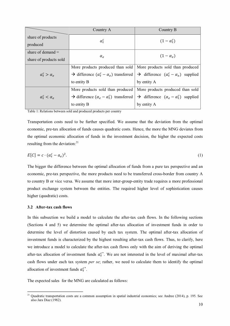
If the share of products sold ( ) is not identical to the share of products produced ( ) by the entity
in country A, entity A either has to buy part of the products from entity B ( > ) or has to supply
entity B with products ( < ). As both companies produce in sum exactly as many products as
demanded in sum in both countries, the surplus of products produced by entity A can be sold to entity
B, which sells them to the customers in country B, and vice versa. By subtracting from we
obtain the share of produced products that exceeds the share of products that can be sold directly by
entity A. Table 1 graphically illustrates these relations.
19 Similarly modelled by Devereux & Griffith (1998), p. 340. 20 Devereux & Griffith (1998), p. 336 also focus on transportation costs as the crucial factor in deciding where to produce.
10
Country A Country B
share of products
produced (1 − )
share of demand =
share of products sold (1 − )
>
More products produced than sold
difference ( − ) transferred
to entity B
More products sold than produced
difference ( − ) supplied
by entity A
<
More products sold than produced
difference ( − ) transferred
to entity B
More products produced than sold
difference ( − ) supplied
by entity A Table 1: Relations between sold and produced products per country
Transportation costs need to be further specified. We assume that the deviation from the optimal
economic, pre-tax allocation of funds causes quadratic costs. Hence, the more the MNG deviates from
the optimal economic allocation of funds in the investment decision, the higher the expected costs
resulting from the deviation:21
[ ] = · ( − ) . (1)
The bigger the difference between the optimal allocation of funds from a pure tax perspective and an
economic, pre-tax perspective, the more products need to be transferred cross-border from country A
to country B or vice versa. We assume that more inter-group-entity trade requires a more professional
product exchange system between the entities. The required higher level of sophistication causes
higher (quadratic) costs.
3.2 After-tax cash flows
In this subsection we build a model to calculate the after-tax cash flows. In the following sections
(Sections 4 and 5) we determine the optimal after-tax allocation of investment funds in order to
determine the level of distortion caused by each tax system. The optimal after-tax allocation of
investment funds is characterized by the highest resulting after-tax cash flows. Thus, to clarify, here
we introduce a model to calculate the after-tax cash flows only with the aim of deriving the optimal
after-tax allocation of investment funds ∗. We are not interested in the level of maximal after-tax
cash flows under each tax system per se; rather, we need to calculate them to identify the optimal
allocation of investment funds ∗.
The expected sales for the MNG are calculated as follows:
21 Quadratic transportation costs are a common assumption in spatial industrial economics; see Andree (2014), p. 195. See
also Jara Diaz (1982).
11
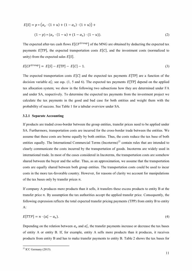
[ ] = ∗ · (1 + ) + (1 − ) · (1 + ) +
(1 − ) ∗ ( · (1 − ) + (1 − ) · (1 − )). (2)
The expected after-tax cash flows [ ] of the MNG are obtained by deducting the expected tax
payments [TP], the expected transportation costs [ ], and the investment costs (normalized to
unity) from the expected sales [ ].
[ ] = [ ] − [TP] − [ ] − 1. (3)
The expected transportation costs [ ] and the expected tax payments [TP] are a function of the
decision variable ; see eqs. (1, 5 and 6). The expected tax payments [TP] depend on the applied
tax allocation system; we show in the following two subsections how they are determined under FA
and under SA, respectively. To determine the expected tax payments from the investment project we
calculate the tax payments in the good and bad case for both entities and weight them with the
probability of success. See Table 1 for a tabular overview under SA.
3.2.1 Separate Accounting
If products are traded cross-border between the group entities, transfer prices need to be applied under
SA. Furthermore, transportation costs are incurred for the cross-border trade between the entities. We
assume that these costs are borne equally by both entities. Thus, the costs reduce the tax base of both
entities equally. The International Commercial Terms (Incoterms)22 contain rules that are intended to
clearly communicate the costs incurred by the transportation of goods. Incoterms are widely used in
international trade. In most of the cases considered in Incoterms, the transportation costs are somehow
shared between the buyer and the seller. Thus, as an approximation, we assume that the transportation
costs are equally shared between both group entities. The transportation costs could be used to incur
costs in the more tax-favorable country. However, for reasons of clarity we account for manipulations
of the tax bases only by transfer prices .
If company A produces more products than it sells, it transfers these excess products to entity B at the
transfer price . By assumption the tax authorities accept the applied transfer price. Consequently, the
following expression reflects the total expected transfer pricing payments (TPP) from entity B to entity
A:
[ ] = · ( − ). (4)
Depending on the relation between and , the transfer payments increase or decrease the tax bases
of entity A or entity B. If, for example, entity A sells more products than it produces, it receives
products from entity B and has to make transfer payments to entity B. Table 2 shows the tax bases for
22 ICC Germany (2015).
12
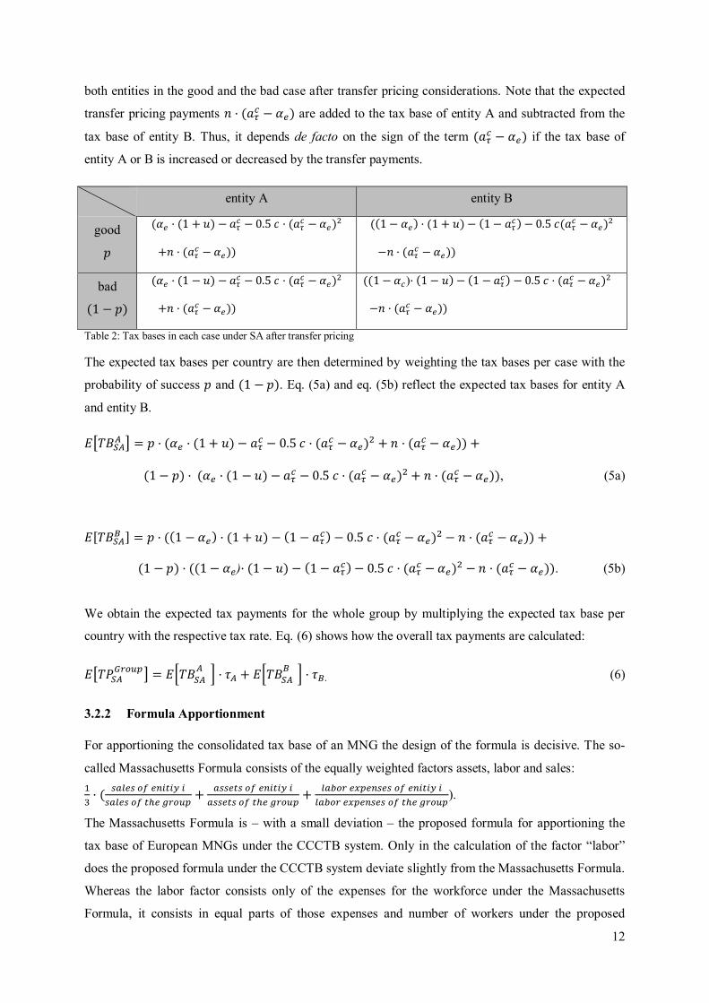
both entities in the good and the bad case after transfer pricing considerations. Note that the expected
transfer pricing payments · ( − ) are added to the tax base of entity A and subtracted from the
tax base of entity B. Thus, it depends de facto on the sign of the term ( − ) if the tax base of
entity A or B is increased or decreased by the transfer payments.
entity A entity B
good
( · (1 + ) − − 0.5 · ( − )
+ · ( − ))
((1 − ) · (1 + ) − (1 − ) − 0.5 ( − )
− · ( − ))
bad
(1 − )
( · (1 − ) − − 0.5 · ( − )
+ · ( − ))
((1 − )· (1 − ) − (1 − ) − 0.5 · ( − )
− · ( − ))
Table 2: Tax bases in each case under SA after transfer pricing
The expected tax bases per country are then determined by weighting the tax bases per case with the
probability of success and (1 − ). Eq. (5a) and eq. (5b) reflect the expected tax bases for entity A
and entity B.
= · ( · (1 + ) − − 0.5 · ( − ) + · ( − )) +
(1 − ) · ( · (1 − ) − − 0.5 · ( − ) + · ( − )), (5a)
[ ] = · ((1 − ) · (1 + ) − (1 − ) − 0.5 · ( − ) − · ( − )) +
(1 − ) · ((1 − )· (1 − ) − (1 − ) − 0.5 · ( − ) − · ( − )). (5b)
We obtain the expected tax payments for the whole group by multiplying the expected tax base per
country with the respective tax rate. Eq. (6) shows how the overall tax payments are calculated:
= · + · . (6)
3.2.2 Formula Apportionment
For apportioning the consolidated tax base of an MNG the design of the formula is decisive. The so-
called Massachusetts Formula consists of the equally weighted factors assets, labor and sales:
· (
+
+
).
The Massachusetts Formula is – with a small deviation – the proposed formula for apportioning the
tax base of European MNGs under the CCCTB system. Only in the calculation of the factor “labor”
does the proposed formula under the CCCTB system deviate slightly from the Massachusetts Formula.
Whereas the labor factor consists only of the expenses for the workforce under the Massachusetts
Formula, it consists in equal parts of those expenses and number of workers under the proposed
13
CCCTB formula. However, this small simplification of the Massachusetts Formula is negligible for
the purpose of our analysis. The Massachusetts Formula was originally used by almost all states in the
US to apportion the consolidated tax base of national groups to the entities. However, whereas under
the proposed CCCTB system the factors are weighted equally, in the US there is room for deviation
from these weights. States tend to give more weight to the sales factor and distribute the remaining
weights equally across the asset and the labor factor. As we focus on the CCCTB setting in this study
we assume fixed and equally weighted factor weights as under the Massachusetts Formula.
Furthermore, we assume that under FA the share of assets is equal to the share of labor for each entity.
The basic idea of this assumption is that assets, e.g., machinery, require a proportional number of
workers to operate them. Thus, they are seen as complements.23 Note that the MNG already has some
well-established business activities that also have to be taken into account when determining the
allocation of the group tax base. The existing shares of assets, labor, and sales per entity induced by
other business activities are assumed to correspond to the shares of these factors that result from the
investment. Thus, the allocation of the group tax base between the entities does not change due to the
investment. Consequently, the variables and contain all necessary information to determine
which share of the group tax base is allocated to which entity.
In contrast to SA, under FA the costs and sales from the investment are consolidated on the group
level. Thus, the MNG cannot benefit from segregating expenses and sales and incurring them
separately in tax-favorable environments. We take the provisions governing FA under the CCCTB
system as a model for this study. According to Section 96 of the CCCTB proposal,24 sales are assigned
to the destination country of the sold products. Thus, under FA, it is generally possible to segregate the
location of sales and the location of assets and labor (i.e., the location of production). Under FA,
segregation is decisive for the tax-optimal arrangement of the apportionment factors between country
A and country B. Note that such a segregation would not be possible if the sales were assigned to the
country where the products were produced. Due to the consolidation of profits and/or losses on the
group level, no transfer pricing issues arise. As a side note, it would not make a difference to the sales
factor if we relax the assumption of prohibiting direct sales in other countries. If we assume that entity
A sells its products directly to the end customers in country B instead of selling them indirectly to
them via entity B, the share of the group tax base allocated to each entity does not have to be adjusted.
The formula apportionment systems that exist around the world offer different ways to deal with
losses. Whereas in the US the overall loss of the group is allocated to the group members and is
carried forward on the entity level, under the European CCCTB system it is not allocated to the group
entities and is carried forward on the group level. However, in the scenario considered here we assume
that the group incurs profits from other business activities so that the overall tax base of the group is
23 See Runkel & Schjelderup (2011), p. 916 and Dietrich & Kiesewetter (2007), p. 507. 24 See European Commission (2011).

14
positive and losses can be offset against profits within the group. Consequently, under this assumption
we do not need to distinguish between a formula apportionment system that does or does not allow for
allocating losses to the entities.
To apply the apportionment formula we need to know which share of sales, assets, and labor accrue in
which country. As described in the section headed “Assumptions”, the variables and (1 − )
represent the shares of sales and the variables and (1 − ) represent the shares of assets and labor
present in each country. The transportation costs do not impact the relative allocation of assets and
labor between the countries. The MNG is assumed to outsource transportation to a logistics company.
The share of assets and labor is assumed to be equal in each country. Thus, the share of the overall tax
base apportioned to country A is calculated as follows
= ( + 2 · ). (7)
Consequently, the share allocated to country B is = (1 − ), respectively.
Due to cross-border consolidation, the expected tax base on the group level is determined by summing
up the results of both group entities:25
= [ ] − [ ] − 1 (8)
= (−1 + 2 ) · − ∗ ( − ).
By multiplying the tax base with the apportionment factors · and · , we obtain the expected
tax payments of the group:
= · ( · + · ). (9)
4 No costs for the segregation of sales and assets/labor
In a first step, we assume that no transportation costs (or costs for language or currency differences)
are incurred for products that are sold within the group. Such a setting would be reasonable for
example in the EU, where two countries have the same currency, have the same official language, and
where intangible products like software are sold by one entity to another. However, a setting without
transportation costs may be more specific than a setting with transportation costs. As we assume no
transportation costs, there is no optimal pre-tax investment decision. From a pre-tax perspective the
group is indifferent to investing in country A or country B. Therefore, in this section we cannot draw
any conclusions about the level of distortion caused by each tax system. However, as a preliminary
step, we can infer which tax allocation system offers stronger incentives to make a tax-optimal
25 Note that unlike under SA, transfer prices do not affect eq. (8).
15
investment decision. The incentive for an optimal investment decision is measured by the additional
tax payments that are caused by a marginal deviation from the optimal after-tax allocation of funds.
The higher the additional marginal tax payments, the higher the incentives to invest optimally. In the
next section we introduce transportation costs and thus are able to draw conclusions about the level of
implied distortions. As the assumption of zero transportation costs slims down the complexity of the
model, it allows us to understand the basic mechanism behind each tax allocation system in depth. It
thus also serves to prepare for the following more complex model setting with transportation costs.
Note that in this section we label our decision variable (not ) as no transportation costs occur.
However, with exception of the transportation costs, the explanations and formulas given in Section 3
for are fully applicable to this section, too.
The after-tax cash flows indicate for which value of the after-tax allocation of funds is optimal
( ∗), i.e., when the after-tax cash flows are maximal. However, in case the transportation costs are
assumed to be zero, we refrain from modeling the after-tax profits explicitly. The investment decision
does not affect the expected pre-tax cash flows ( = [ ] − 1) but only the tax
payments. Thus, as tax payments are the only dimension that is affected by the decision variable ,
here we focus only on tax payments. The after-tax cash flows can be easily determined by subtracting
the tax payments from the pre-tax cash flows of the MNG. The higher the tax payments, the lower the
after-tax cash flows.
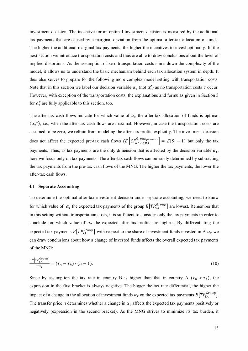
4.1 Separate Accounting
To determine the optimal after-tax investment decision under separate accounting, we need to know
for which value of the expected tax payments of the group are lowest. Remember that
in this setting without transportation costs, it is sufficient to consider only the tax payments in order to
conclude for which value of the expected after-tax profits are highest. By differentiating the
expected tax payments with respect to the share of investment funds invested in A we
can draw conclusions about how a change of invested funds affects the overall expected tax payments
of the MNG:
= ( − ) · ( − 1). (10)
Since by assumption the tax rate in country B is higher than that in country A ( > ), the
expression in the first bracket is always negative. The bigger the tax rate differential, the higher the
impact of a change in the allocation of investment funds on the expected tax payments .
The transfer price determines whether a change in affects the expected tax payments positively or
negatively (expression in the second bracket). As the MNG strives to minimize its tax burden, it
16
strategically sets transfer prices in order to benefit from tax rate differentials.26 Anecdotal and
empirical evidence gives us an idea of how MNGs de facto set their transfer prices in a scenario as
assumed in our model.27 A statement by the former chief financial officer of the automotive
manufacturer BMW suggests that BMW strategically attempted to uncouple the location of expenses
from the location of sales. At a press conference on financial statements, the CFO announced that the
company attempted to accrue expenses wherever the tax rates were highest.28 Subsequently, top
executives at BASF and Merck referred to the tax organization of BMW as a role model for their own
groups.29 Based on those statements, Feld (2000) states that MNGs have opportunities to incur costs in
that country with the relative higher tax rate and use income-shifting channels like transfer pricing
structures to incur profits in low-tax countries. Empirical evidence found by Egger et al. (2010)
supports Feld’s finding that MNGs attach particular importance to the costs of an investment when
choosing the investment location. They find evidence that in Europe, profit shifting seems to be more
pronounced than debt shifting. As MNGs have an incentive to separate investment costs from the
resulting sales for tax purposes, and as it seems to be easier for them to shift the resulting sales than
the costs, the investment is ideally carried out in a high-tax country and the resulting sales are then
shifted to low-tax countries. Consequently, MNGs seem to focus on placing the real activity (i.e., labor
and assets) in a favorable high-tax tax environment if they have an opportunity to shift income.
There is also some empirical evidence that indicates that MNGs are able to uncouple the costs of an
investment from the resulting sales. Grubert (2003) finds that MNGs invest either in extra-low- or in
extra-high-tax countries if they have good opportunities for income-shifting. MNGs invest in extra-
low-tax countries to establish a destination for the shifted income and in extra high-tax countries to
benefit from high tax refunds on the resulting losses of the investment. Note that in our setting there is
already a company in a low-tax country to which income can be shifted (entity A). Thus, in line with
the findings of Grubert, the MNG aims to carry out the real investment in the high-tax country and
may shift potential income to the low-tax country in our setting. The empirical evidence found by
Overesch (2009) supports Grubert’s results. Based on German panel data for inbound investments he
finds evidence that real investment in high-tax countries is positively affected by a lower taxation of
income shifted abroad. The results of an analytical study by Hong and Smart (2010) points in the same
direction. They suggest that the possibility to shift income to tax havens makes the MNG less
responsive to tax rate differentials when choosing the location where the investment shall be carried
out.
26 See Dietrich & Kiesewetter (2011), p. 101. 27 As both entities are assumed to produce identical products and sell them to end customers at the same expected price, at
first glance it seems reasonable to use this expected price as the transfer price.27 However, the expected price is only an estimated value for planning purposes and will certainly not occur, as the investment develops either positively or negatively. Thus, the expected market price cannot serve as a reasonable benchmark for the transfer price.
28 Doppelfeld cited by Schaefer, (1993) p. 2. 29 Weichenrieder (1996), p. 38.
17
There is also analytical evidence that indicates explicitly that MNGs try to incur costs or losses in
high-tax countries. Results found by Becker and Fuest (2007) indicate that MNGs try to carry out real
investments in high-tax countries if marginal profits are allowed to be negative. In our model the
MNG incurs negative or zero marginal profits in the high-tax country since it shifts profits away.
Becker and Fuest state that in such case higher taxes may attract more real investment. They argue that
strategic investments in non-profitable projects could explain why the stock of foreign capital held in
Germany increased tremendously between 1990 and 2000 even though the corporate tax rate was very
high during that period. Haufler and Strähler (2013)’s argument for low tax bases in high-tax countries
points in the same direction. They argue that firms rank their entities according to profitability.
According to their line of argumentation, highly profitable low-cost entities settle in low-tax countries,
which are usually fairly small. By contrast, high-cost entities settle in large, high-tax countries.
All in all, we infer from these studies that MNGs can geographically uncouple the expenses and sales
of an investment. The most complete segregation between costs and sales is achieved when one entity
produces all products and gives them free of charge to the other group entity, which sells them. Note
that in our model the location of sales is determined by local demand and can be neither changed nor
optimized. By contrast, the location of production can be determined by the MNG via the share of
funds invested in the production process (in labor and assets, ) in each country. If the producing
entity offers the products free of charge to the selling company, the transfer price takes on a value of
zero ( = 0). If the producing entity sells the products to the selling company at its production costs,
the transfer price amounts to one ( = 1). The transfer price is the only means for income-shifting in
our model. We assume that the transfer price captures all possible income-shifting channels.30 Besides
shifting income via transfer pricing, the MNG could shift income, e.g., by internal debt31 or by royalty
payments. We assume comprehensive income-shifting opportunities so that the MNG is in any case
able to set transfer prices that are smaller than or equal to one (0 ≤ ≤ 1).
Eq. (10) illustrates that an increase in increases the expected tax payments if is
smaller than one ( < 1). In that case the entity, which produces more products than it sells to end
customers, sells the remaining products to the other group entity at a price that is lower than the
production costs. As follows from eq. (10), the partial derivative is strictly monotonously decreasing
in if < 1. As the definition range for is given by the interval [0,1], i.e, 0 ≤ ≤ 1, the lowest
expected tax payments/the highest tax refunds occur for = 0. That is to say, all investment funds
are invested in country B. This conclusion is intuitive. As we assume an immediate and full loss-
offset, the expected tax payments are lowest if as many investment-related expenses as possible are
incurred in the high-tax country and – in case of successful development – if at the same time as much
profits as possible are shifted to and taxed in the low-tax country. The more the transfer price
30 See Grubert & Mutti (1991), p. 286. 31 See Dietrich & Kiesewetter (2011), p. 101.
18
approaches zero, the lower the expected tax payments or the higher the expected tax refunds,
respectively. Thus, MNGs try to negotiate transfer prices in such a way that these are as low as
possible. Furthermore, the closer the transfer price is to zero, the higher the expected tax payments
with an increase in .
Moreover, eq. (10) shows that in the case of a transfer price that is equal to the production costs
( = 1) the partial derivative with respect to is equal to zero. Consequently, a marginal change in
the allocation of investment funds does not impact the expected tax payments. Thus, the expected
tax payments/expected tax refunds are independent of the value of . The intuitive explanation
therefore is that at = 1 the MNG is not able to allocate the investment costs between the two
countries and thus it cannot strategically accrue losses in the tax-favorable environments. A value of
= 1 does not offer any scope for tax-motivated income-shifting.
4.2 Formula Apportionment
To get an idea of how the allocation of investment funds affects the expected tax
payments/expected tax refunds under FA, we calculate the partial derivative of eq. (8)
with respect to :
= · ( − ) · (−1 + 2 ) · . (11)
The tax rate differential in the first brackets is by definition always positive. The variable is by
definition also always positive. Thus, only the probability of a successful production determines if
the marginal change in the allocation of investment funds affects the expected tax payments
negatively or positively. If the probability of success is exactly one half ( = 0.5), then
has no influence on the expected tax payments. That is intuitive as the expected tax base is then
zero. If the probability of success is smaller than 0.5 ( < 0.5) we obtain an expected loss from the
investment project. It follows from eq. (11) that in such a case, an increase in the share of investment
funds in country A increases the expected tax payments. Thus, as the partial derivative shown in eq.
(11) is strictly monotonously decreasing if < 0.5, the MNG would be best advised to invest all funds
in country B ( = 0). Under an immediate and full loss-offset, the expected tax payments for the
MNG are lowest if all losses are allocated to the high-tax country B. In country B the tax refunds for
the losses are highest. If is greater than 0.5 ( > 0.5), the investment generates expected profits. In
such a case, an increase in decreases the expected tax payments since the partial derivative of eq.
(11) is strictly monotonously increasing, so the MNG should invest all funds in A ( = 1).32 The
expected tax payments for the MNG are lowest if all profits are allocated to and taxed in the low-tax
country A.
32 See Dietrich & Kiesewetter (2007), p. 514.
19
4.3 Comparison of both tax allocation systems with respect to the incentives to invest optimally
A substantial difference between both tax allocation systems is that under FA the tax-favorable
allocation of investment funds depends on whether the investment project is expected to be profitable
or not. If the MNG expects a profit and invests the funds in line with this expectation but finally incurs
a loss, the allocation of investment funds turns out to be worst from a tax perspective. By contrast, the
optimal allocation of investment funds under SA does not depend on whether the MNG incurs profits
or losses. As a side note, we refer always to the optimal investment decision from an after-tax
perspective in this section as there is no optimal pre-tax investment decision (remember = 0). Due to
the possibility to segregate costs and sales, under SA, the MNG should always invest all funds in the
high-tax country. Thus, in a profit scenario both tax allocation systems create opposing investment
incentives, while in a loss scenario the incentives are identical. Our main goal in this section is to find
out which tax allocation system creates stronger incentives (i.e., higher tax payments in case of a
marginal deviation from the optimal after-tax allocation of funds) to invest optimally.
By comparing the partial derivatives for the expected tax payments with respect to with each other
(eq. (10) and eq. (11)), it becomes evident under which system a potential misallocation of funds
results in higher expected tax payments. To be more precise, we can infer from comparing eq. (10)
with eq. (11) under which tax allocation system a marginal deviation from the optimal tax-allocation
of funds ∗ results in a stronger increase in expected tax payments. The stronger the increase in tax
payments with a deviation from the tax-optimal allocation of funds, the stronger the incentives to
invest tax-optimally. The partial derivative with respect to under SA is greater than under FA if the
following condition holds:
< · (3 − 2 · + 4 · · ). (12)
Under that condition the MNG has to pay more taxes for a marginal deviation from the optimal
allocation of investment funds ∗ under SA than under FA. Consequently, the incentives under SA
are stronger than those under FA to allocate the investment funds optimally between both countries
from an after-tax perspective. Vice versa, the incentives are stronger under FA if the following
condition holds: > · (3 − 2 · + 4 · · ). The relative distortive power of either tax allocation
system depends on the relation between the transfer price and the expected sales · .
To get an idea of which tax allocation system offers stronger incentives to make an optimal investment
decision, we determine realistic parameter settings. According to CSI Market33 the pre-tax margin for
US companies currently ranges between about 21% in the healthcare sector and about 5% in the retail
sector. We take the median of this range (13%) as the expected average realistic pre-tax margin in our
33 See CSI Market (2015).
20
analysis, allowing us to deduce a variety of possible combinations of and that lead to an expected
pre-tax rate of return of 13%. For example, this is true for = 1 and = 0.13 (setting I) and = 0.6
and = 0.65 (setting II). For all combinations of and that lead to a pre-tax margin of 0.13, the
incentives for an optimal allocation of investment funds are greater under SA than under FA if
< 1.08667. As by assumption ≤ 1, this relation always holds. The same interpretation, e.g., holds
true for a pre-tax margin of 21% (healthcare sector, < 1.14) or 5% (retail sector, < 1.03). Thus, if
the expectations of pre-tax margins are in line with currently observable sector margins of US
companies, the incentives for an optimal allocation of investment funds are always stronger under SA
than under FA.
Note that so far we have not been able to draw conclusions about the distortive effects of each tax
allocation system with respect to locational investment decisions as there has been no optimal pre-tax
investment decision ( = 0). The MNG has been assumed to be indifferent between investing in entity
A or B from a pre-tax perspective. In the following section we change this assumption. By assuming
transportation costs the MNG is no longer indifferent in the pre-tax allocation of investment funds.
Thus, by introducing an optimal allocation of investment funds in the pre-tax scenario, we are able to
draw conclusions about the distortional power of either tax allocation system.
5 Costs for the segregation of sales and assets/labor
So far we have determined the MNG’s optimal allocation of investment funds across countries A and
B assuming no transportation costs. Thus, until now taxation has been the only crucial determinant for
deciding where to invest. Now we expand this setting and assume transportation costs incurred by the
geographical segregation of sales and asset/labor (production). Hence, in this section the transportation
costs are an additional determinant of the optimal investment decision. From a purely pre-tax
perspective, the MNG should invest in entity A and entity B relative to demand in country A and
country B ( ∗) in order to avoid transportation costs.
The occurrence of an optimal allocation of investment funds from a pre-tax perspective ( ∗) creates a
trade-off between the optimal allocation of investment funds from a tax perspective and from a pre-tax
perspective. Transportation costs force the MNG to weigh the economic pre-tax benefits against the
taxation benefits to arrive at a final investment decision ( ∗).34 Thus, the unidimensional optima from
either a tax perspective or a pre-tax perspective are merged to form an overall, multidimensional
optimum( ∗). The transportation costs reduce not only the overall cash flows of the MNG but also
the tax base.35 Thus, it is necessary to explicitly model not only the tax payments – as in Section 4 –
but the entire after-tax cash flows. Note that the main goal of this analysis is to find out the optimal
34 Devereux & Griffith (1998) make a similar assumption. However, in their model transportation costs are weighed up
against gains from economies of scale. 35 Also assumed by Devereux & Griffith (1998), p. 340.

21
after-tax allocation of investment funds ∗ (i.e., the allocation that leads to highest after-tax cash
flows) in order to determine the distortional power of each tax base allocation system.
5.1 Separate Accounting
Under SA the allocation of the transportation costs between both entities is crucial for the tax
payments of the MNG. The transportation costs ( · ( − ) ) have opposing effects on the
expected after-tax cash flows . On the one hand, they decrease the pre-tax profits; on the
other hand, they decrease the tax base and thus the tax payments. However, the impact of the decrease
in tax payments is in any case smaller than the decrease in pre-tax cash flows. Thus, the tax base effect
of the transportation costs is smaller than the pre-tax effect. To find the optimal allocation of
investment funds ∗ the MNG has to weigh up the benefits from a tax-optimal allocation of funds
against the benefits from an economically favorable allocation of funds (i.e., an allocation that results
in low transportation costs). As the transportation costs are assumed to be quadratic, they start at a
very low level and then increase rapidly. At a specific critical the benefits of a tax-favorable
allocation of investment funds are outweighed by the transportation costs. Given quadratic
transportation costs, the expected after-tax cash flows (after transportation costs) decrease with an
increasing deviation from the optimal after-tax allocation of funds ∗. Thus, the curve reflecting the
expected after-tax cash flows [ ] (see eq. (3)) depending on is bell-shaped.
Differentiating eq. (3) with respect to shows how a change in the decision variable impacts the
expected after-tax profits:
= ( − ) · (1 − ) + ( + ) · · ( − ) + 2 · ( − ). (13)
The symbols (“-/0” , “+/0” and “+/-/0“) under the braces indicate the potential signs the expression can
take in accordance with the model assumptions. The allocation of funds is optimal if the partial
derivative of eq. (13) is equal to zero for a value of ∗ that lies within a range of zero and one
(0 ≤ ∗ ≤ 1). Note that the (mathematical) optimum (i.e. where = 0) need not
necessarily lie in this economically reasonable area (0 ≤ ≤ 1). In such a case, ∗ takes the
extreme values of zero if the (mathematical) optimum occurs for values of smaller than zero or of
one if the (mathematical) optimum occurs for values of bigger than one. We can draw this
conclusion as the curve reflecting the expected after-tax results [ ] (see eq. (3)) in
dependence of is bell-shaped.
II I
+/-/0 +/0 -/0 +/0 +/-/0
22
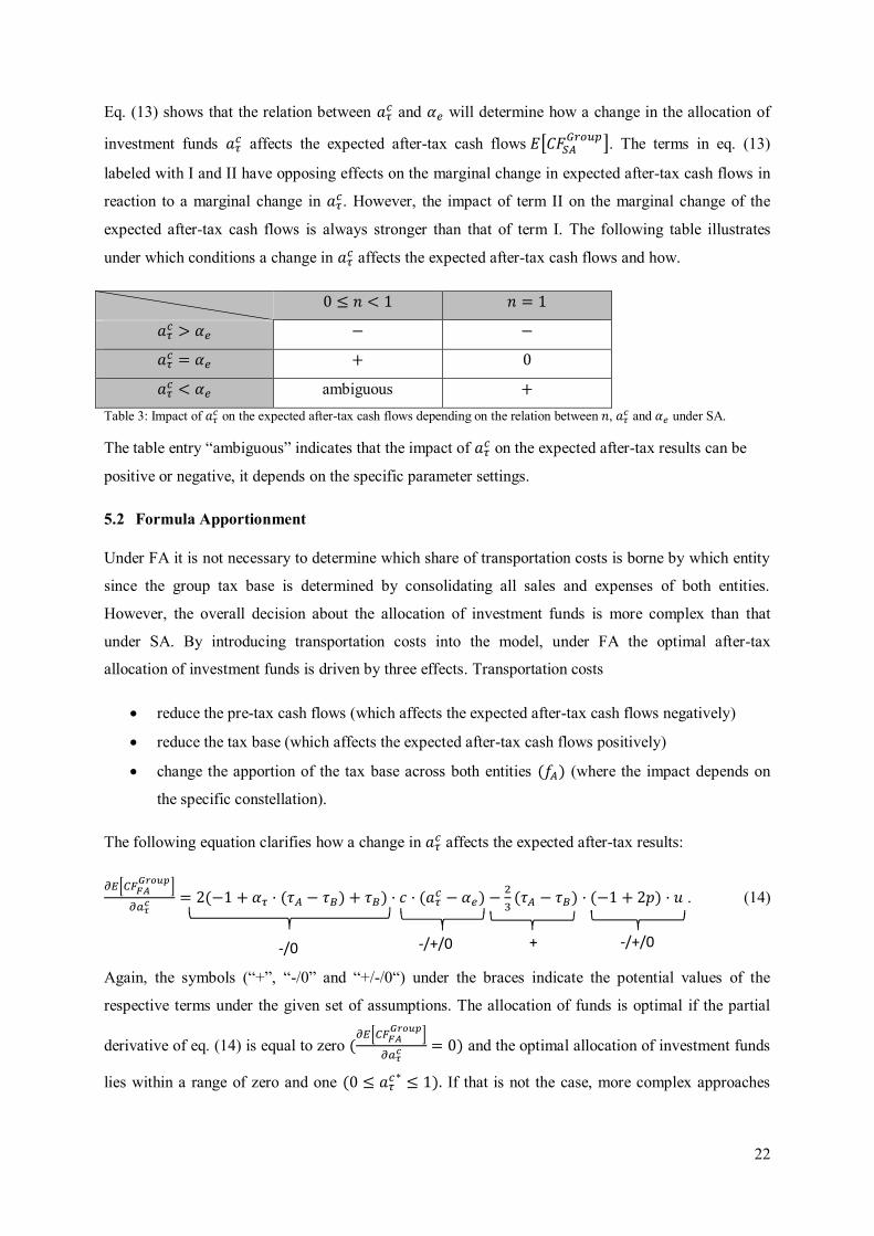
Eq. (13) shows that the relation between and will determine how a change in the allocation of
investment funds affects the expected after-tax cash flows . The terms in eq. (13)
labeled with I and II have opposing effects on the marginal change in expected after-tax cash flows in
reaction to a marginal change in . However, the impact of term II on the marginal change of the
expected after-tax cash flows is always stronger than that of term I. The following table illustrates
under which conditions a change in affects the expected after-tax cash flows and how.
0 ≤ < 1 = 1
> − −
= + 0
< ambiguous + Table 3: Impact of on the expected after-tax cash flows depending on the relation between , and under SA.
The table entry “ambiguous” indicates that the impact of on the expected after-tax results can be
positive or negative, it depends on the specific parameter settings.
5.2 Formula Apportionment
Under FA it is not necessary to determine which share of transportation costs is borne by which entity
since the group tax base is determined by consolidating all sales and expenses of both entities.
However, the overall decision about the allocation of investment funds is more complex than that
under SA. By introducing transportation costs into the model, under FA the optimal after-tax
allocation of investment funds is driven by three effects. Transportation costs
reduce the pre-tax cash flows (which affects the expected after-tax cash flows negatively)
reduce the tax base (which affects the expected after-tax cash flows positively)
change the apportion of the tax base across both entities ( ) (where the impact depends on
the specific constellation).
The following equation clarifies how a change in affects the expected after-tax results:
= 2(−1 + · ( − ) + ) · · ( − ) − ( − ) · (−1 + 2 ) · . (14)
Again, the symbols (“+”, “-/0” and “+/-/0“) under the braces indicate the potential values of the
respective terms under the given set of assumptions. The allocation of funds is optimal if the partial
derivative of eq. (14) is equal to zero ( = 0) and the optimal allocation of investment funds
lies within a range of zero and one (0 ≤ ∗ ≤ 1). If that is not the case, more complex approaches
-/+/0 + -/+/0 -/0

23
have to be applied to find the optimum within the definition area of (0 ≤ ≤ 1).36 Under FA the
relation between , and determines whether affects the expected after-tax results positively
or negatively. The probability of success determines if the investment leads to an expected after-tax
profit or loss. We show already in subsection 4.3 that under FA, the sign of the expected after-tax cash
flows of the MNG (determined by ) is decisive for the optimal investment decision. Table 4 shows
under which conditions a marginal change in affects the expected after-tax cash flows and how.
< 0.5 = 0.5 > 0.5
> − − ambiguous
= − 0 +
< ambiguous + + Table 4: Impact of on the expected after-tax cash flows depending the relation between , and under FA.
If, for example, > and < 0.5, an increase in reduces the expected after-tax cash flows.
The table entry “ambiguous” indicates that the impact of on the expected after-tax results is
ambiguous and depends on the specific parameter settings.
Under SA the expected after-tax cash flows decrease when deviates more strongly from the optimal
after-tax allocation of investment funds ∗ (bell-shaped curve, see subsection 5.1). Under FA that
relation does not necessarily hold (under FA the curve is not necessarily bell-shaped). This is due to
the rather complex impact of on the expected tax payments. Whereas under SA the introduction of
transportation costs impacts the tax payments solely through the decreased tax base, under FA more
complex interrelations between the tax base and its allocation impact the tax payments. Thus, with
respect to the tax payments, an increasing difference between and ∗ may be up to a critical value
of beneficial as higher costs reduce the tax payments. However, if that critical value of is
exceeded, the favorable tax base effects may be outweighed by an unfavorable allocation of the group
tax base to the entities (i.e., extensive losses are allocated to the low-tax country or extensive profits to
the high-tax country).
5.3 Comparison of distortional effects of both tax allocation systems
The introduction of transportation costs affects the locational decisions under FA in more dimensions
than under SA. In addition to the expected pre-tax profits and the tax base, the allocation of the tax
base between the group entities is affected as well. Under one of the following conditions the expected
after-tax cash flows (after transportations costs) are higher under SA than under FA:
< and < 6 + 3 c · − 4 c · − 3 · + 2 c · · + 2 − 4 + 8 (15a)
36 Note that the curve of depending on is not necessarily bell-shaped (as it is under SA). Thus, finding the
maxima within the definition area of (0 ≤ ≤ 1) is not that straightforward if the following condition does not hold
within the definition area: = 0.
24
or
> and > 6 + 3 c · − 4 c · − 3 · + 2 c · · + 2 − 4 + 8 . (15b)
However, the main goal of this analysis is to find out the optimal after-tax allocation of investment
funds ∗ (i.e. the allocation that leads to highest after-tax cash flows) in order to compare that
allocation with the optimal pre-tax allocation. From this comparison we learn which tax allocation
system has stronger distortional effects.
To draw economically meaningful conclusions given the rather complex models, we fall back on a
numerical analysis. In a first step, we determine reasonable and realistic parameter settings. In
subsection 4.4 we already explain reasonable values for the parameters and in line with recent pre-
tax margins (median of 13%) of companies in various sectors. In the period 1990-2008 average
transportation costs for industry and trade ranged between 7% and 27% of total costs.37 To account for
realistic tax rate differentials we take the highest and lowest tax rates within EU member states (i.e.,
Slovenia with 17% and France with 34.43%) for 2015.38 As we believe that the fraction of income that
the MNG is able to shift to the low-tax country A under SA is highly dependent on the industry and
the characteristics of the MNG, we refrain from attaching a value to . We apply the same
argumentation for not attaching a value to the optimal pre-tax allocation of investment funds ∗. In
Fig. (1), we show for three levels (“low”, “medium”, “high”) of ∗ and under which system the
distortion of the optimal investment decisions is more severe. The vertical black line in Fig. (1)
indicates the optimal pre-tax allocation of investment funds.
Fig. (1) shows the expected after-tax cash flows depending on the after-tax allocation of investment
funds . The tax allocation system that leads to a bigger difference between the optimal pre-tax
allocation of funds ∗ and the optimal after-tax allocation of funds is identified as the more
distortive system. Remember that the optimal after-tax allocation of funds is characterized by the
maximal after-tax cash flows. The upper abbreviation (SA or FA) in the framed boxes above each
graph indicates under which tax allocation system the distortions of the investment decision are
greater. The lower abbreviation indicates which system leads to the higher expected after-tax cash
flows in the optimum. The latter information is not directly relevant for our research question yet it is
an interesting side note. The parameter constellations in Fig. (1) are chosen in such a way that, under
optimal allocation of investment funds, the investment project is profitable under either system. Note
that the curves for FA in Fig. (1) do not change with changing income-shifting possibilities
(represented by the level of the transfer price ) as transfer pricing only exists under SA.
Fig. (1) shows that the distortions tend to be greater under SA than under FA for better possibilities of
income-shifting (decreasing value of ) and for a higher share of funds that is optimally invested in 37 Statista (2015). 38 We use the combined corporate income tax rate. OECD (2015).

25
entity A in the pre-tax case (increasing value of ∗) under SA. The income-shifting possibilities
determine the level of distortion under SA. The better the income-shifting possibilities (the lower ),
i.e., the stricter the local segregation of costs and sales, the more the MNG can benefit from a tax-
favorable allocation of funds. Consequently, it is worthwhile for the MNG to deviate more from the
optimal pre-tax allocation ∗ to approach the optimal tax allocation ∗ for its final investment
decision ( ∗ ). High transportation costs for a greater deviation from ∗ are refunded by high tax
savings in case of good income-shifting possibilities. Remember from the no-cost scenario in Section
4 that the optimal allocation of funds from a tax perspective is always extreme. Under SA the optimal
allocation is ∗ = 0 while under FA it is ∗ = 1 in a profit situation.
The greater the difference between the unidimensional optima ∗ and ∗ under each tax allocation
system, the greater the resulting distortions with respect to the final investment decision ∗. This is
because due to the quadratic transportation costs the MNG surrenders only few pre-tax profits for a
small deviation from ∗ but greatly reduces its taxes by choosing an after-tax allocation of
investment funds ∗ that is closer to ∗. The optimal investment decision ∗ is reached if the
marginal tax savings are equal to the marginal transportation costs. In line with that explanation, Fig.
(1) shows that the distortions of the investment decisions are greatest under SA and lowest under FA
for high values of ∗. In such a case the difference between the unidimensional optima ( ∗, ∗) are
highest under SA and lowest under FA. Vice versa, for low values of ∗ the difference between the
unidimensional optima ( ∗, ∗) is low under SA and high under FA and thus the distortion tends to
be higher under FA.
The results do not change qualitatively with respect to the relative distortion caused by each tax
allocation system if we vary the transportation costs , the profitability (determined by and , as
long as they ensure still a profitable setting) or the tax rate differential ( − ) within economically
reasonable ranges (see Appendix 1-3). However, in the following we change our setting from a profit
to a loss scenario (changing the probability of a successful investment outcome from 0.6 to 0.1, see
Fig. (2)). To consider an investment project which results in an expected after-tax loss needs to be
justified in our model set-up as a rational executive of an MNG would not invest in such a project
from the outset.
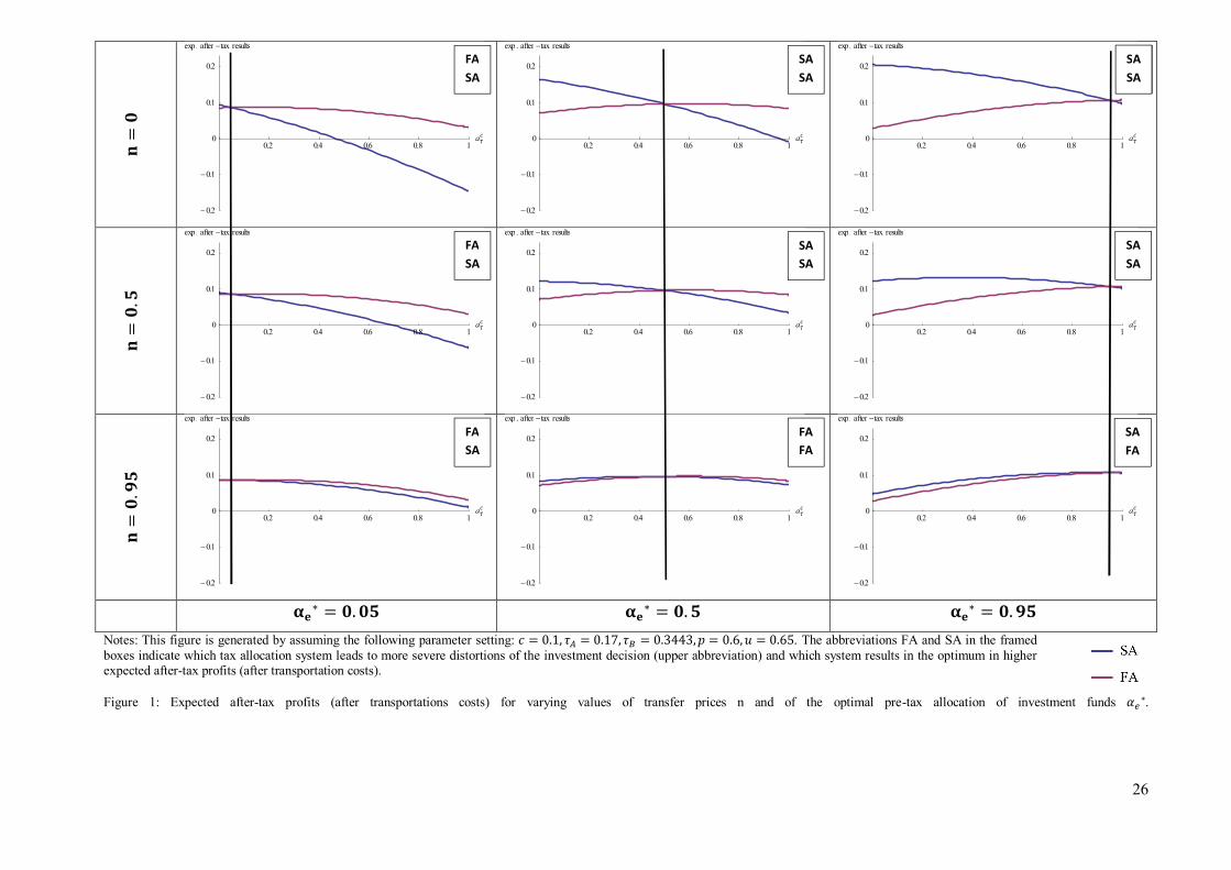
26
=
=.
=.
∗ = . ∗ = . ∗ = . Notes: This figure is generated by assuming the following parameter setting: = 0.1, = 0.17, = 0.3443, = 0.6, = 0.65. The abbreviations FA and SA in the framed boxes indicate which tax allocation system leads to more severe distortions of the investment decision (upper abbreviation) and which system results in the optimum in higher expected after-tax profits (after transportation costs).
Figure 1: Expected after-tax profits (after transportations costs) for varying values of transfer prices n and of the optimal pre-tax allocation of investment funds ∗.
0.2 0.4 0.6 0.8 1a
c
0.2
0.1
0
0.1
0.2
exp. aftertax results
0.2 0.4 0.6 0.8 1a
c
0.2
0.1
0
0.1
0.2
exp. aftertax results
0.2 0.4 0.6 0.8 1a
c
0.2
0.1
0
0.1
0.2
exp. aftertax results
0.2 0.4 0.6 0.8 1a
c
0.2
0.1
0
0.1
0.2
exp. aftertax results
0.2 0.4 0.6 0.8 1a
c
0.2
0.1
0
0.1
0.2
exp. aftertax results
0.2 0.4 0.6 0.8 1a
c
0.2
0.1
0
0.1
0.2
exp. aftertax results
0.2 0.4 0.6 0.8 1a
c
0.2
0.1
0
0.1
0.2
exp. aftertax results
0.2 0.4 0.6 0.8 1a
c
0.2
0.1
0
0.1
0.2
exp. aftertax results
0.2 0.4 0.6 0.8 1a
c
0.2
0.1
0
0.1
0.2
exp. aftertax results
FA SA
FA FA
SA FA
FA SA
FA SA
SA SA
SA SA
SA SA
SA SA
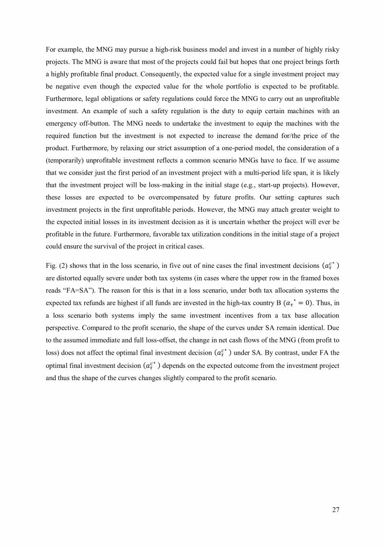
27
For example, the MNG may pursue a high-risk business model and invest in a number of highly risky
projects. The MNG is aware that most of the projects could fail but hopes that one project brings forth
a highly profitable final product. Consequently, the expected value for a single investment project may
be negative even though the expected value for the whole portfolio is expected to be profitable.
Furthermore, legal obligations or safety regulations could force the MNG to carry out an unprofitable
investment. An example of such a safety regulation is the duty to equip certain machines with an
emergency off-button. The MNG needs to undertake the investment to equip the machines with the
required function but the investment is not expected to increase the demand for/the price of the
product. Furthermore, by relaxing our strict assumption of a one-period model, the consideration of a
(temporarily) unprofitable investment reflects a common scenario MNGs have to face. If we assume
that we consider just the first period of an investment project with a multi-period life span, it is likely
that the investment project will be loss-making in the initial stage (e.g., start-up projects). However,
these losses are expected to be overcompensated by future profits. Our setting captures such
investment projects in the first unprofitable periods. However, the MNG may attach greater weight to
the expected initial losses in its investment decision as it is uncertain whether the project will ever be
profitable in the future. Furthermore, favorable tax utilization conditions in the initial stage of a project
could ensure the survival of the project in critical cases.
Fig. (2) shows that in the loss scenario, in five out of nine cases the final investment decisions ( ∗ )
are distorted equally severe under both tax systems (in cases where the upper row in the framed boxes
reads “FA=SA”). The reason for this is that in a loss scenario, under both tax allocation systems the
expected tax refunds are highest if all funds are invested in the high-tax country B ( ∗ = 0). Thus, in
a loss scenario both systems imply the same investment incentives from a tax base allocation
perspective. Compared to the profit scenario, the shape of the curves under SA remain identical. Due
to the assumed immediate and full loss-offset, the change in net cash flows of the MNG (from profit to
loss) does not affect the optimal final investment decision ( ∗ ) under SA. By contrast, under FA the
optimal final investment decision ( ∗ ) depends on the expected outcome from the investment project
and thus the shape of the curves changes slightly compared to the profit scenario.
28
=
=.
=.
∗ = . ∗ = . ∗ = . Notes: This figure is generated by assuming the following parameter settings: = 0.1, = 0.17, = 0.3443, = 0.4, = 0.65. The abbreviations FA and SA in the framed boxes indicate which tax allocation system leads to more severe distortions of the investment decision (upper abbreviation) and which system results in the optimum in higher expected after-tax profits (after transportation costs).
Figure 2: Expected after-tax losses (after transportations costs) for varying values of transfer prices n and of the optimal pre-tax allocation of investment funds ∗.
0.2 0.4 0.6 0.8 1a
c0
0.1
0.2
0.3
0.4
exp. aftertax results
0.2 0.4 0.6 0.8 1a
c0
0.1
0.2
0.3
0.4
exp. aftertax results
0.2 0.4 0.6 0.8 1a
c0
0.1
0.2
0.3
0.4
exp. aftertax results
0.2 0.4 0.6 0.8 1a
c0
0.1
0.2
0.3
0.4
exp. aftertax results
0.2 0.4 0.6 0.8 1a
c0
0.1
0.2
0.3
0.4
exp. aftertax results
0.2 0.4 0.6 0.8 1a
c0
0.1
0.2
0.3
0.4
exp. aftertax results
0.2 0.4 0.6 0.8 1a
c0
0.1
0.2
0.3
0.4
exp. aftertax results
0.2 0.4 0.6 0.8 1a
c0
0.1
0.2
0.3
0.4
exp. aftertax results
0.2 0.4 0.6 0.8 1a
c0
0.1
0.2
0.3
0.4
exp. aftertax results
SA SA
FA=SA SA
FA=SA SA
FA=SA FA
FA=SA SA
FA FA
FA FA
FA=SA SA
SA SA
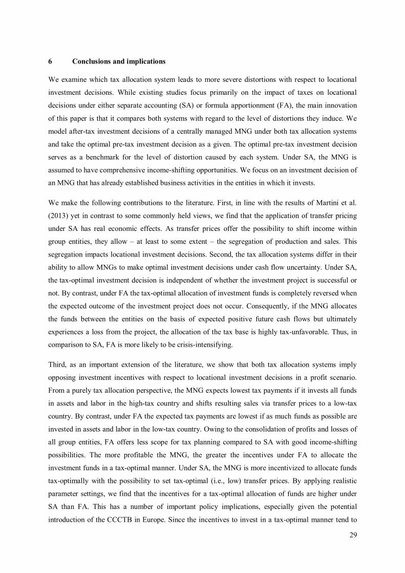
29
6 Conclusions and implications
We examine which tax allocation system leads to more severe distortions with respect to locational
investment decisions. While existing studies focus primarily on the impact of taxes on locational
decisions under either separate accounting (SA) or formula apportionment (FA), the main innovation
of this paper is that it compares both systems with regard to the level of distortions they induce. We
model after-tax investment decisions of a centrally managed MNG under both tax allocation systems
and take the optimal pre-tax investment decision as a given. The optimal pre-tax investment decision
serves as a benchmark for the level of distortion caused by each system. Under SA, the MNG is
assumed to have comprehensive income-shifting opportunities. We focus on an investment decision of
an MNG that has already established business activities in the entities in which it invests.
We make the following contributions to the literature. First, in line with the results of Martini et al.
(2013) yet in contrast to some commonly held views, we find that the application of transfer pricing
under SA has real economic effects. As transfer prices offer the possibility to shift income within
group entities, they allow – at least to some extent – the segregation of production and sales. This
segregation impacts locational investment decisions. Second, the tax allocation systems differ in their
ability to allow MNGs to make optimal investment decisions under cash flow uncertainty. Under SA,
the tax-optimal investment decision is independent of whether the investment project is successful or
not. By contrast, under FA the tax-optimal allocation of investment funds is completely reversed when
the expected outcome of the investment project does not occur. Consequently, if the MNG allocates
the funds between the entities on the basis of expected positive future cash flows but ultimately
experiences a loss from the project, the allocation of the tax base is highly tax-unfavorable. Thus, in
comparison to SA, FA is more likely to be crisis-intensifying.
Third, as an important extension of the literature, we show that both tax allocation systems imply
opposing investment incentives with respect to locational investment decisions in a profit scenario.
From a purely tax allocation perspective, the MNG expects lowest tax payments if it invests all funds
in assets and labor in the high-tax country and shifts resulting sales via transfer prices to a low-tax
country. By contrast, under FA the expected tax payments are lowest if as much funds as possible are
invested in assets and labor in the low-tax country. Owing to the consolidation of profits and losses of
all group entities, FA offers less scope for tax planning compared to SA with good income-shifting
possibilities. The more profitable the MNG, the greater the incentives under FA to allocate the
investment funds in a tax-optimal manner. Under SA, the MNG is more incentivized to allocate funds
tax-optimally with the possibility to set tax-optimal (i.e., low) transfer prices. By applying realistic
parameter settings, we find that the incentives for a tax-optimal allocation of funds are higher under
SA than FA. This has a number of important policy implications, especially given the potential
introduction of the CCCTB in Europe. Since the incentives to invest in a tax-optimal manner tend to

30
be lower under FA, the tax-optimal allocation of funds is less important under that system. That is
desirable from a tax policy perspective as it tends to distort pre-tax investment decisions to a lesser
extent. However, only by considering specific optimal pre-tax investment decisions can we draw
conclusions about the level of distortion caused by either system.
Finally, by introducing costs for the geographical segregation of production and sales, we can draw
conclusions about the level of distortions induced by each tax allocation system. The distortions under
SA tend to be more severe than under FA if a greater share of investment funds is to be invested in a
low-tax country from a pre-tax perspective and the investment is profitable. In such a setting, the
MNG would deviate rather strongly from the optimal pre-tax investment decision in order to benefit
from a more tax-favorable environment. Such pre-tax investment decisions are typical for German
MNGs (particularly those in the manufacturing industry) that invest e.g. in low-tax Eastern European
countries to gain access to a low-wage workforce.39 The after-tax investment decision tends to be
distorted more severely under SA than under FA if comprehensive income-shifting opportunities
under SA are assumed. Vice versa, pre-tax decisions that result in the investment of a big share of
funds in the high-tax country tend to be distorted less under SA than under FA. R&D investments in
the pharmaceutical industry may be a model for such pre-tax investment decisions. MNGs need highly
skilled and well-educated workers and seek a very high level of legal certainty to maintain a hold over,
e.g., their patents. Such conditions are typical for the European high-tax countries such as Germany,
France, or Belgium.
From our results we can derive some important policy implications. The introduction of the CCCTB in
Europe may have a tremendous impact on locational investment decisions and the shifting of
economic substance to low-tax countries.40 It depends on the sector in question how well an MNG is
able to adjust the company structure to reverse investment incentives under FA. While a company in
the manufacturing industry may be able to easily adjust to incentives offered by FA, companies in the
pharmaceutical industry may find this more difficult.
Our findings must be interpreted against the background of our set of assumptions. Our results are
driven by the assumption that MNGs have ample opportunity to shift income to low-tax countries
under SA. Even if we validate this assumption by empirical, anecdotal, and analytical evidence, it may
not be appropriate for all MNGs. Several important issues have not yet been sufficiently addressed. It
is a rather strong assumption to assume quadratic transportation costs. It would be desirable to test our
results under different cost functions, too. Furthermore, it would be interesting to examine distortional
effects under both tax allocation systems if the assumption of a direct loss-offset is dropped.
39 See Devereux (2008), p. 636. 40 See Devereux (2008), p. 636.
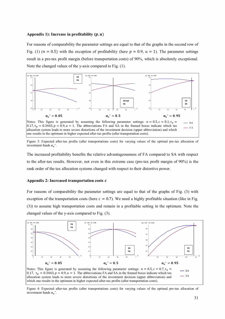
31
Appendix 1): Increase in profitability ( , )
For reasons of comparability the parameter settings are equal to that of the graphs in the second row of
Fig. (1) ( = 0.5) with the exception of profitability (here = 0.9, = 1). The parameter settings
result in a pre-tax profit margin (before transportation costs) of 90%, which is absolutely exceptional.
Note the changed values of the y-axis compared to Fig. (1).
∗ = . ∗ = . ∗ = .
Notes: This figure is generated by assuming the following parameter settings: = 0.5, = 0.1, =0.17, = 0.3443, = 0.9, = 1. The abbreviations FA and SA in the framed boxes indicate which tax allocation system leads to more severe distortions of the investment decision (upper abbreviation) and which one results in the optimum in higher expected after-tax profits (after transportation costs).
Figure 3: Expected after-tax profits (after transportations costs) for varying values of the optimal pre-tax allocation of investment funds α ∗.
The increased profitability benefits the relative advantageousness of FA compared to SA with respect
to the after-tax results. However, not even in this extreme case (pre-tax profit margin of 90%) is the
rank order of the tax allocation systems changed with respect to their distortive power.
Appendix 2: Increased transportation costs
For reasons of comparability the parameter settings are equal to that of the graphs of Fig. (3) with
exception of the transportation costs (here = 0.7). We need a highly profitable situation (like in Fig.
(3)) to assume high transportation costs and remain in a profitable setting in the optimum. Note the
changed values of the y-axis compared to Fig. (3).
∗ = . ∗ = . ∗ = .
Notes: This figure is generated by assuming the following parameter settings: = 0.5, = 0.7, =0.17, = 0.3443, = 0.9, = 1. The abbreviations FA and SA in the framed boxes indicate which tax allocation system leads to more severe distortions of the investment decision (upper abbreviation) and which one results in the optimum in higher expected after-tax profits (after transportation costs).
Figure 4: Expected after-tax profits (after transportations costs) for varying values of the optimal pre-tax allocation of investment funds α ∗.
0 0.2 0.4 0.6 0.8 1a
c0.3
0.4
0.5
0.6
0.7exp . aftertax results
0 0.2 0.4 0.6 0.8 1a
c0.3
0.4
0.5
0.6
0.7exp. aftertax results
0 0.2 0.4 0.6 0.8 1a
c0.3
0.4
0.5
0.6
0.7exp. aftertax results
0 0.2 0.4 0.6 0.8 1a
c0
0.1
0.2
0.3
0.4
0.5
0.6
0.7exp . aftertax results
0 0.2 0.4 0.6 0.8 1a
c0
0.1
0.2
0.3
0.4
0.5
0.6
0.7exp. aftertax results
0.2 0.4 0.6 0.8 1.0a
c
0.2
0.3
0.4
0.5
0.6
exp . aftertax results
FA=SA FA
SA FA
SA SA
SA FA
FA FA
FA FA
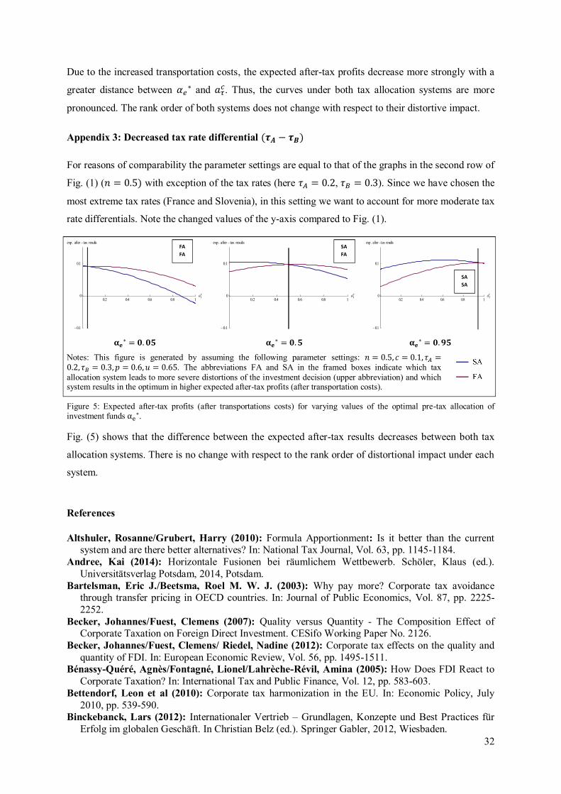
32
Due to the increased transportation costs, the expected after-tax profits decrease more strongly with a
greater distance between ∗ and . Thus, the curves under both tax allocation systems are more
pronounced. The rank order of both systems does not change with respect to their distortive impact.
Appendix 3: Decreased tax rate differential ( − )
For reasons of comparability the parameter settings are equal to that of the graphs in the second row of
Fig. (1) ( = 0.5) with exception of the tax rates (here = 0.2, = 0.3). Since we have chosen the
most extreme tax rates (France and Slovenia), in this setting we want to account for more moderate tax
rate differentials. Note the changed values of the y-axis compared to Fig. (1).
∗ = . ∗ = . ∗ = .
Notes: This figure is generated by assuming the following parameter settings: = 0.5, = 0.1, =0.2, = 0.3, = 0.6, = 0.65. The abbreviations FA and SA in the framed boxes indicate which tax allocation system leads to more severe distortions of the investment decision (upper abbreviation) and which system results in the optimum in higher expected after-tax profits (after transportation costs).
Figure 5: Expected after-tax profits (after transportations costs) for varying values of the optimal pre-tax allocation of investment funds α ∗.
Fig. (5) shows that the difference between the expected after-tax results decreases between both tax
allocation systems. There is no change with respect to the rank order of distortional impact under each
system.
References
Altshuler, Rosanne/Grubert, Harry (2010): Formula Apportionment: Is it better than the current system and are there better alternatives? In: National Tax Journal, Vol. 63, pp. 1145-1184.
Andree, Kai (2014): Horizontale Fusionen bei räumlichem Wettbewerb. Schöler, Klaus (ed.). Universitätsverlag Potsdam, 2014, Potsdam.
Bartelsman, Eric J./Beetsma, Roel M. W. J. (2003): Why pay more? Corporate tax avoidance through transfer pricing in OECD countries. In: Journal of Public Economics, Vol. 87, pp. 2225-2252.
Becker, Johannes/Fuest, Clemens (2007): Quality versus Quantity - The Composition Effect of Corporate Taxation on Foreign Direct Investment. CESifo Working Paper No. 2126.
Becker, Johannes/Fuest, Clemens/ Riedel, Nadine (2012): Corporate tax effects on the quality and quantity of FDI. In: European Economic Review, Vol. 56, pp. 1495-1511.
Bénassy-Quéré, Agnès/Fontagné, Lionel/Lahrèche-Révil, Amina (2005): How Does FDI React to Corporate Taxation? In: International Tax and Public Finance, Vol. 12, pp. 583-603.
Bettendorf, Leon et al (2010): Corporate tax harmonization in the EU. In: Economic Policy, July 2010, pp. 539-590.
Binckebanck, Lars (2012): Internationaler Vertrieb – Grundlagen, Konzepte und Best Practices für Erfolg im globalen Geschäft. In Christian Belz (ed.). Springer Gabler, 2012, Wiesbaden.
0.2 0.4 0.6 0.8 1a
c
0.1
0
0.1
exp. aftertax results
0.2 0.4 0.6 0.8 1a
c
0.1
0
0.1
exp. aftertax results
0.2 0.4 0.6 0.8 1a
c
0.1
0
0.1
exp. aftertax resultsFA FA
SA SA
SA FA

33
Binet, Marie-Estelle (2008): Optimal local taxation and French municipal tax distortions. In: Applied Economics, Vol. 40, pp. 327-332.
Buettner, Thiess (2002): The impact of taxes and public spending on the location of FDI: Evidence from FDI-flows within Europe. ZEW Discussion Paper 02-17, Mannheim.
Buettner, Thiess/Wamser, Georg (2013): Internal debt and multinational profit shifting: Empirical evidence from firm-level panel data. In: National Tax Journal, Vol. 66, pp. 63-96.
Clausing, Kimberly A. (2009): Multinational firm tax avoidance and tax policy. In: National Tax Journal, Vol. 62, No. 4, pp. 703-725.
CSI market (2015): Pre-tax margin screening. Web. 22 Oct. 2015. http://csimarket.com/screening/index.php?s=pm&pageS=4&fis= (date of last access: 22 Oct 2015).
Dahle, Claudia (2011): Der Einfluss von Mindestbesteuerungskonzepten auf unternehmerische Investitionsentscheidungen unter Berücksichtigung grenzüberschreitender Gruppenbesteuerungs-systeme. Verlag Dr. Kovač, 2011, Hamburg.
Devereux, Michael P./Griffith, Rachel (1998): Taxes and the location of production: evidence from a panel of US multinationals. In: Journal of Public Economics, Vol. 68, pp. 335-367.
Devereux, Michal P./Maffini, Giorgia (2006): The Impact of Taxation on the Location of Capital, Firms and Profit: A Servey of Empirical Evidence. Oxford University Centre for Business Taxation WP 07/02.
Devereux, Michael P. (2008): Business taxation in a globalized world. In: Oxford Review of Economic Policy, Vol. 24, pp. 625-638.
Dharmapala, Dhammika (2014): What Do We Know about Base Erosion and Profit Shifting? A Review of the Empirical Literature. Coase-Sandor Institute for Law and Economics, Working Paper No. 702.
Dietrich, Maik/Kiesewetter, Dirk (2007): Auswirkungen einer Common Consolidated Tax Base bei Investitionsentscheidungen der Multinationalen Unternehmung. In: Betriebswirtschaftliche Forschung und Praxis, Vol. 59, pp. 498-516.
Dietrich, Maik/Kiesewetter, Dirk (2011): Simultane Investitions- und Finanzierungsentscheidungen einer multinationalen Unternehmung bei Anwendung des Einheitsprinzips. In: Betriebswirtschaftliche Forschung und Praxis, Vol. 63, pp. 101-117.
Dischinger, Matthias/Knoll, Bodo/Riedel, Nadine (2014): The role of headquarters in multinational profit shifting strategies. In: International Tax and Public Finance, Vol. 21, pp. 248-271.
Dyreng, Scott/Markle, Kevin (2013): The Effect of Financial Constraints on Tax-Motivated Income Shifting by U.S. Multinationals. DOI: http://dx.doi.org/10.2139/ssrn.2336799.
Egger, Peter/Eggert, Wolfgang/Winner, Hannes (2010): Saving taxes through foreign plant ownership. In: Journal of International Economics, Vol. 81, pp. 99-108.
European Commission (2011): Proposal for a Council Directive on a Common Consolidated Corporate Tax Base (CCCTB). COM (2011) 121/4.
Feld, Lars P. (2000): Steuerwettbewerb und seine Auswirkungen auf Allokation und Distribution – Ein Überblick und eine empirische Analyse für die Schweiz. Mohr Siebeck, 2000, Tübingen.
Fuest, Clemens (2008): The European Commission’s proposal for a common consolidated corporate tax base. In: Oxford Review of Economic Policy, Vol. 24, pp. 720-739.
Fuest, Clemens/Hemmelgarn, Thomas/Ramb, Fred (2007): How would the introduction of an EU-wide formula apportionment affect the distribution and size of the corporate tax base? An analysis based on German multinationals. In: International Tax and Public Finance, Vol. 14, pp. 605-626.
Gordon, Roger/Wilson, John D. (1986): An Examination of Multijurisdictional Corporate Income Taxation under Formula Apportionment. In: Econometrica, Vol. 54, pp. 1357-1373.
Gorter, Joeri/Parikh, Ashok (2003): How sensitive is FDI to differences in corporate income taxation within the EU? In: De Economist Vol. 151, pp. 193-204.
Goolsbee, Austan/Maydew, Edward L. (2000): Coveting thy neighbor`s manufacturing: The dilemma of state income apportionment. In: Journal of Public Economics, Vol. 75, pp.125-143.
Grubert, Harry (2003): Intangible Income, Intercompany Transactions, Income Shifting, and the Choice of Lacation. In: National Tax Journal, Vol. 56, pp. 221-242.
Grubert, Harry/Mutti, John (1991): Taxes, Tariffs and Transfer Pricing in Multinational Corporate Decision Making. In: The Review of Economics and Statistics, Vol. 73, pp. 285-293.
34
Grubert, Harry/Slemrod, Joel (1998): The Effect of Taxes on Investment and Income Shifting to Puerto Rico. In: Review of Economics and Statistics, Vol. 73, pp. 365-373.
Harris, David/Morck, Randall/Slemrod, Joel/Bernard Yeung (1993): The Impact of US tax law revision on multinational companies. In: Journal of Accounting Research (Supplement), Vol. 31, pp. 111-140.
Haufler, Andreas/Stähler, Frank (2013): Tax Competition a Simple Model with Heterogeneous Firms: How larger Markets reduce Profit Taxes. In: International Economic Review, Vol. 54, pp. 665-692.
Heckemeyer, Jost H./Overesch, Michael (2013): Multinationals’ Profit Response to Tax Differentials: Effect Size and Shifting Channels. ZEW Discussion Paper No. 13-045, Mannheim.
Hong, Qing/Smart, Michael (2009): In praise of tax havens: International tax planning and foreign direct investment. In: European Economic Review, Vol. 54, pp. 82-95.
Huizinga, Harry/Laeven, Luc (2007): International profit shifting within multinationals: A multi-country perspective. In: Journal of Public Economics, Vol. 92, pp. 1164-1182.
ICC Germany (2015): ICC Incoterms 2010. Web. 22 Oct. 2015. http://www.iccgermany.de/icc-regeln-und-richtlinien/icc-incotermsR-2010-ueberblick.html (date of last access: 22 Oct. 2015).
Jara Diaz, Sergio R. (1982): The estimation of transport costs function: a methodological review. In: Transport Reviews, Vol. 2, pp. 257-278.
Kiesewetter, Dirk/Steigenberger, Tobias/Stier, Matthias (2014): Can formula apportionment really prevent multinational enterprises from profit shifting? – The role of asset valuation, intragroup debt and leases. arqus Discussion Paper No. 175.
Kruschwitz, Lutz/Schneider, Dirk/Husmann, Sven (2003): Investitionsneutrale Steuersysteme unter Sicherheit. In: Wissenschaftliches Studium, Vol. 32 (2003), pp. 328-333.
Mintz, Jack/Smart, Michael (2004): Income shifting, investment, and tax competition: theory and evidence from provincial taxation in Canada. In. Journal of Public Economics, Vol. 88, pp. 1149-1168.
Nielsen, Søren Bo/Raimondos-Møller, Pascalis/Schjelderup, Guttorm (2003): Formula Apportionment and Transfer Pricing under Oligopolistic Competition. In: Journal of Public Economic Theory, Vol. 5, pp. 419-437.
Nielsen, Søren Bo/Raimondos-Møller, Pascalis/Schjelderup, Guttorm (2010): Company taxation and tax spillovers: Separate accounting versus formula apportionment. In: European Economic Review, Vol. 54, pp. 121-132.
OECD (2013): Action Plan on Base Erosion and Profit Shifting. OECD Publishing, Paris 2013. DOI: http://dx.doi.org/10.1787/9789264202719-en.
OECD (2015): OECD.Stat – Corporate Income Tax Rate. Web. 22. Oct. 2015. http://stats.oecd.org//Index.aspx?QueryId=58204 (date of last access: 22 Oct 2015).
Oestreicher, Andreas/Koch, Reinald (2011): The Revenue Consequences of Using a Common Consolidated Corporate Tax Base to Determine Taxable Income in the EU Member States. In: FinanzArchiv, Vol. 67, pp. 64-102.
Ortmann, Regina/Sureth-Sloane, Caren (2016): Can the CCCTB Alleviate Tax Discrimination against Loss-making European Multinational Groups? In: Journal of Business Economics, forthcoming.
Overesch, Michael (2009): The Effects of Multinationals’ Profit Shifting Activities on Real Investments. In: National Tax Journal, Vol. 62, pp. 5-23.
Runkel, Marco/Schjelderup, Guttorm (2011): On the Choice of Apportionment Factors under Formula Apportionment. In: International Economic Review, Vol. 52(3), pp. 913-934.
Schaefer, Waldemar (1993): BMW zahlt kaum noch Ertragsteuern im Inland. Zu Lasten des Staates. In: Handelsblatt, 26.03.1993, p. 2.
Statista (2015): Anteil der Logistikkosten an den Gesamtkosten. http://de.statista.com/statistik/daten/studie/6346/umfrage/anteil-der-logistikkosten-an-den-gesamtkosten/ (date of last access: 22 Oct. 2015).
Uniform Division of Income for Tax Purposes Act (1966). Web 3. Nov. 2015. http://www.uniformlaws.org/shared/docs/uditpa/uditpa66.pdf (date of last access: 3 Nov. 2015).
Weichenrieder, Alfons (1996): Fighting International Tax Avoidance: The case of Germany. In: Fiscal Studies, Vol. 17, pp. 37-58.