Orthogonal Polynomials,

Perturbed Hankel Determinants

and

Random Matrix Models

A thesis presented for the degree of

Doctor of Philosophy of Imperial College London

and the

Diploma of Imperial College

by

Nazmus Saqeeb Haq

Department of Mathematics

Imperial College

180 Queen’s Gate, London SW7 2BZ

September 2013

2

I certify that this thesis, and the research to which it refers, are the product of my own work,

and that any ideas or quotations from the work of other people, published or otherwise, are

fully acknowledged in accordance with the standard referencing practices of the discipline.

Signed: N. S. Haq

3

Copyright

The copyright of this thesis rests with the author and is made available under a Creative

Commons Attribution Non-Commercial No Derivatives licence. Researchers are free to copy,

distribute or transmit the thesis on the condition that they attribute it, that they do not use it

for commercial purposes and that they do not alter, transform or build upon it. For any reuse

or redistribution, researchers must make clear to others the licence terms of this work.

4

To my friends and family.

5

Abstract

In this thesis, for a given weight function w(x), supported on [A,B] ⊆ R, we consider the

sequence of monic polynomials orthogonal with respect to w(x), and the Hankel determinant

Dn = det(μj+k)n−1j,k=0, generated from the moments μj of w(x). A motivating factor for studying

such objects is that by observing the Andreief-Heine identity, these determinants represent the

partition function of a Hermitian random matrix ensemble.

It is well known that the Hankel determinant can be computed via the product of L2 norms

over [A,B] ⊆ R of the orthogonal polynomials associated with w(x). Since such polynomials sat-

isfy a three-term recurrence relation, we also study the behaviour of the recurrence coefficients,

denoted by αn and βn, as these are intimately related to the behaviour of Dn.

We consider orthogonal polynomials and Hankel determinants associated with the following

two weight functions:

First, we consider a deformation of the Jacobi weight, given by

w(x) = (1 − x2)α(1 − k2x2)β , x ∈ [−1, 1], α > −1, β ∈ R, k2 ∈ (0, 1).

This is a generalization of a system of orthogonal polynomials studied by C. J. Rees in 1945.

Such orthogonal polynomials are of great interest because the corresponding Hankel determinant

is related to the τ -function of a Painleve VI differential equation, the special cases of which are

related to enumerative problems arising from String theory.

For finite n—we employ the orthogonal polynomial ladder operators (formulae that raise

or lower the index of the polynomial) to find equations for auxiliary quantities defined by the

corresponding orthogonal polynomials, from which we derive differential identities satisfied by

the Hankel determinant, and differential-difference identities for the recurrence coefficients αn

and βn.

6

Making use of the ladder operators, we find that the recurrence coefficient βn(k2), n =

1, 2, . . . ; and p1(n, k2), the coefficient of xn−2 of the corresponding monic orthogonal polyno-

mials, satisfy second order non-linear difference equations. The large n expansion based on the

difference equations when combined Toda-type differential relations satisfied by the associated

Hankel determinant yields a complete asymptotic expansion of Dn. The finite n representation

of Dn in terms of a particular Painleve VI equation is also discussed as well as the generalization

of the linear second order differential equation found by Rees.

Second, we consider the deformed Laguerre weight:

w(x) = xαe−x(t+ x)Ns (T + x)−Ns , x ∈ [0,∞), α > −1, T, t,Ns > 0.

This weight is of interest since it appears in the study of a multiple-antenna wireless communi-

cation scenario. The key quantity determining system performance is the statistical properties

of the signal-to-noise ratio (SNR) γ, which recent work has characterized through its moment

generating function, in terms of the Hankel determinant generated via our deformed Laguerre

weight.

We make use of the ladder operators to give an exact finite n characterization of the Hankel

determinant in terms of a two-variable generalization of a Painleve V differential equation,

which reduces to Painleve V under certain limits.

We also employ Dyson’s Coulomb fluid theory to derive an approximation for Dn—in the

limit where n is large. The finite and large n characterizations are then used to compute closed-

form (non-determinantal) expressions for the cumulants of the distribution of γ, and to compute

wireless communication performance quantities of engineering interest.

7

Acknowledgements

I would like to express my thanks to Prof. Yang Chen for his support, guidance and especially

patience over the last few years. I appreciate that he always gave very generously of his time

(sometimes up to eight hours in a single day!) and as a result taught me many invaluable

lessons.

I would like to thank Prof. Matthew R. McKay, Prof. Estelle L. Basor and Dr Igor Krasovsky

for their contribution to the material presented in this thesis, and their additional support and

input.

To Andita and Farrah for all their help and constructive criticisms during the past year:

Thank You!

Thanks to Christopher Green, Arman Sahovic and Olasunkanmi Obanubi for some useful

discussions throughout the years (for Arman: the decade); and also for the memories. Thanks

to friends old and new who have made the last few years go by in the blink of an eye, especially

Andita Shantikatara, Ariadne Whitby and Guiyi Ho.

I would like to thank my various sources of financial support. Funding from the Engineering

and Physical Sciences Research Council (EPSRC), has made this research possible. I would

also like to thank ESPCI ParisTech, Columbia University and the Institute for Mathematical

Sciences at the National University of Singapore for their hospitality during my stay there.

Finally, I cannot forget the love and support of my parents, Thank You for putting up with

me!

Saqeeb

8

Table of Contents

Abstract 5

Acknowledgements 7

List of Figures 11

List of Tables 11

List of Publications 12

1 Introduction 131.1 A Brief Background to the Theory of Random Matrices . . . . . . . . . . . . . . 131.2 Random Matrices and Hankel Determinants . . . . . . . . . . . . . . . . . . . . . 141.3 Orthogonal Polynomial and Coulomb Fluid Representations . . . . . . . . . . . . 18

1.3.1 Orthogonal Polynomials and Ladder Operators . . . . . . . . . . . . . . . 181.3.2 Coulomb Fluid Representation . . . . . . . . . . . . . . . . . . . . . . . . 201.3.3 Alternative Representations . . . . . . . . . . . . . . . . . . . . . . . . . . 20

1.4 Outline of Thesis . . . . . . . . . . . . . . . . . . . . . . . . . . . . . . . . . . . . 21

2 Characterization of Hankel Determinant Using Orthogonal Polynomials 252.1 Representations of Hankel Determinant . . . . . . . . . . . . . . . . . . . . . . . 252.2 Construction of Orthogonal Polynomials . . . . . . . . . . . . . . . . . . . . . . . 272.3 Polynomials Orthogonal with Respect to an Even Weight Function . . . . . . . . 292.4 Ladder Operators and Compatibility Conditions . . . . . . . . . . . . . . . . . . 30

3 Coulomb Fluid Model 333.1 Preliminaries of the Coulomb Fluid Method . . . . . . . . . . . . . . . . . . . . . 343.2 Coulomb Fluid Approximation for Hankel Determinant . . . . . . . . . . . . . . 37

4 Deformed Jacobi Weight and Generalized Elliptic Orthogonal Polynomials 384.1 Heine and Rees . . . . . . . . . . . . . . . . . . . . . . . . . . . . . . . . . . . . . 384.2 Outline of Chapter . . . . . . . . . . . . . . . . . . . . . . . . . . . . . . . . . . . 414.3 Summary of Results . . . . . . . . . . . . . . . . . . . . . . . . . . . . . . . . . . 424.4 Computation of Auxiliary Variables . . . . . . . . . . . . . . . . . . . . . . . . . 46

4.4.1 Difference Equations from Compatibility Conditions . . . . . . . . . . . . 474.4.2 Analysis of Non-Linear System . . . . . . . . . . . . . . . . . . . . . . . . 48

4.5 Non-Linear Difference Equation for βn . . . . . . . . . . . . . . . . . . . . . . . . 504.5.1 Proof of Theorem 4.1 . . . . . . . . . . . . . . . . . . . . . . . . . . . . . 504.5.2 Proof of Theorem 4.2 . . . . . . . . . . . . . . . . . . . . . . . . . . . . . 524.5.3 Proof of Theorem 4.3 . . . . . . . . . . . . . . . . . . . . . . . . . . . . . 53

4.6 Second Order Difference Equations for βn and p1(n) . . . . . . . . . . . . . . . . 554.6.1 Proof of Theorem 4.4 . . . . . . . . . . . . . . . . . . . . . . . . . . . . . 56

9

4.6.2 Proof of Theorem 4.5 . . . . . . . . . . . . . . . . . . . . . . . . . . . . . 574.6.3 Proof of Theorem 4.6 . . . . . . . . . . . . . . . . . . . . . . . . . . . . . 57

4.7 Special Solutions of the Non-Linear Difference Equations for βn . . . . . . . . . . 624.7.1 Reduction to Jacobi Polynomials: Third Order Difference Equation . . . 624.7.2 Extension to k2 = −1 . . . . . . . . . . . . . . . . . . . . . . . . . . . . . 644.7.3 Reduction to Jacobi Polynomials: Second Order Difference Equation . . . 654.7.4 Fixed Points of the Second Order Equation . . . . . . . . . . . . . . . . . 66

4.8 Large n Expansion of βn and p1(n) . . . . . . . . . . . . . . . . . . . . . . . . . . 664.8.1 Large n Expansion of Second Order Difference Equation for βn . . . . . . 674.8.2 Large n Expansion of Higher Order Difference Equations for βn . . . . . . 714.8.3 Large n Expansion of Second Order Difference Equation for p1(n) . . . . 72

4.9 Large n Expansion of Hankel determinant . . . . . . . . . . . . . . . . . . . . . . 734.9.1 Alternative Methodologies . . . . . . . . . . . . . . . . . . . . . . . . . . . 734.9.2 Computation of Asymptotic Expansion for Dn . . . . . . . . . . . . . . . 754.9.3 Toda Evolution . . . . . . . . . . . . . . . . . . . . . . . . . . . . . . . . . 764.9.4 Toda Evolution of Hankel Determinant . . . . . . . . . . . . . . . . . . . 764.9.5 Proof of Theorem 4.15 . . . . . . . . . . . . . . . . . . . . . . . . . . . . . 77

4.10 Painleve VI Representation for Hankel Determinant . . . . . . . . . . . . . . . . 794.10.1 Proof of Theorem 4.7 . . . . . . . . . . . . . . . . . . . . . . . . . . . . . 80

4.11 Summary of Chapter . . . . . . . . . . . . . . . . . . . . . . . . . . . . . . . . . . 82

5 Deformed Laguerre Weights and Wireless Relaying 845.1 MIMO Wireless Systems . . . . . . . . . . . . . . . . . . . . . . . . . . . . . . . . 84

5.1.1 Outline of Chapter . . . . . . . . . . . . . . . . . . . . . . . . . . . . . . . 865.1.2 Wireless Communication Performance Measures . . . . . . . . . . . . . . 87

5.2 Statistical Characterization of the SNR γ . . . . . . . . . . . . . . . . . . . . . . 885.2.1 Alternative Characterization of the SNR γ . . . . . . . . . . . . . . . . . 92

5.3 Painleve Characterization via the Ladder Operator Framework . . . . . . . . . . 935.4 Asymptotic Limits of Hankel Determinant . . . . . . . . . . . . . . . . . . . . . . 96

5.4.1 T → ∞ and t→ ∞ . . . . . . . . . . . . . . . . . . . . . . . . . . . . . . . 965.4.2 Statistical Characterization of SNR as Ns → ∞ . . . . . . . . . . . . . . . 96

5.5 Coulomb Fluid Method For Large n Analysis . . . . . . . . . . . . . . . . . . . . 985.5.1 Coulomb Fluid Calculations for the SNR Moment Generating Function . 98

5.6 Coulomb Fluid Analysis of Large n Cumulants of SNR . . . . . . . . . . . . . . . 1015.7 Analysis of Cumulants Using Painleve Characterization . . . . . . . . . . . . . . 103

5.7.1 Initial Conditions . . . . . . . . . . . . . . . . . . . . . . . . . . . . . . . . 1055.7.2 Finite n Analysis of κ1 . . . . . . . . . . . . . . . . . . . . . . . . . . . . . 1065.7.3 Large n Analysis of κ1 . . . . . . . . . . . . . . . . . . . . . . . . . . . . . 1075.7.4 Finite n Analysis of κ2 . . . . . . . . . . . . . . . . . . . . . . . . . . . . . 1095.7.5 Large n Analysis of κ2 . . . . . . . . . . . . . . . . . . . . . . . . . . . . . 1105.7.6 Beyond κ1 and κ2 . . . . . . . . . . . . . . . . . . . . . . . . . . . . . . . 1125.7.7 Comparison of Cumulants Obtained from ODEs with those Obtained from

Determinant Representation . . . . . . . . . . . . . . . . . . . . . . . . . . 1135.8 SER Performance Measure Analysis Based on Coulomb Fluid . . . . . . . . . . . 1145.9 Asymptotic Performance Analysis Based on Coulomb Fluid . . . . . . . . . . . . 116

5.9.1 The Case of β = 0 . . . . . . . . . . . . . . . . . . . . . . . . . . . . . . . 1165.9.2 The Case of β 6= 0 (with NR < ND) . . . . . . . . . . . . . . . . . . . . . 120

5.10 Characterizing A0 Through Painleve V . . . . . . . . . . . . . . . . . . . . . . . . 1235.11 Summary of Chapter . . . . . . . . . . . . . . . . . . . . . . . . . . . . . . . . . . 127

10

6 Summary 1296.1 Discussion of Chapter 4 . . . . . . . . . . . . . . . . . . . . . . . . . . . . . . . . 1296.2 Discussion of Chapter 5 . . . . . . . . . . . . . . . . . . . . . . . . . . . . . . . . 1316.3 Final Remarks . . . . . . . . . . . . . . . . . . . . . . . . . . . . . . . . . . . . . 132

A Painleve Equations 134A.1 Hamiltonian Structure . . . . . . . . . . . . . . . . . . . . . . . . . . . . . . . . . 135A.2 Associated τ -Functions and σ-Forms . . . . . . . . . . . . . . . . . . . . . . . . . 136

B Coefficients of Second Order Difference Equation for βn 138

C Toeplitz+Hankel Determinants 141

D Amplify-and-Forward Wireless Relay Model 144D.1 Preliminaries . . . . . . . . . . . . . . . . . . . . . . . . . . . . . . . . . . . . . . 144D.2 Instantaneous Signal-to-Noise Ratio γ . . . . . . . . . . . . . . . . . . . . . . . . 146D.3 Derivation of Moment Generating Function Mγ(s) . . . . . . . . . . . . . . . . . 147

E Proof of Theorem 5.1 148E.1 Computation of Auxiliary Variables . . . . . . . . . . . . . . . . . . . . . . . . . 148E.2 Difference Equations from Compatibility Conditions . . . . . . . . . . . . . . . . 149E.3 Analysis of Non-linear System . . . . . . . . . . . . . . . . . . . . . . . . . . . . . 151E.4 Toda Evolution . . . . . . . . . . . . . . . . . . . . . . . . . . . . . . . . . . . . . 152E.5 Toda Evolution of Hankel Determinant . . . . . . . . . . . . . . . . . . . . . . . . 155E.6 Partial Differential Equation for Hn(T, t) . . . . . . . . . . . . . . . . . . . . . . 158

F Proof of Theorem 5.2 160F.1 Computation of Auxiliary Variables . . . . . . . . . . . . . . . . . . . . . . . . . 160F.2 Difference Equations from Compatibility Conditions . . . . . . . . . . . . . . . . 161F.3 Analysis of Non-linear System . . . . . . . . . . . . . . . . . . . . . . . . . . . . . 162F.4 Toda Evolution . . . . . . . . . . . . . . . . . . . . . . . . . . . . . . . . . . . . . 163F.5 Toda Evolution of Hankel Determinant . . . . . . . . . . . . . . . . . . . . . . . . 165F.6 Partial Differential Equation for Hn(ξ, η) . . . . . . . . . . . . . . . . . . . . . . . 166

G Some Relevant Integral Identities 168

H Differential Equations For Large n Corrections To Cumulants 171H.1 κ2(t′) . . . . . . . . . . . . . . . . . . . . . . . . . . . . . . . . . . . . . . . . . . . 171H.2 κ3(t′) . . . . . . . . . . . . . . . . . . . . . . . . . . . . . . . . . . . . . . . . . . . 172

I Large n Correction Coefficients For Cumulants 173I.1 κ2(t′) . . . . . . . . . . . . . . . . . . . . . . . . . . . . . . . . . . . . . . . . . . . 173I.2 κ3(t′) . . . . . . . . . . . . . . . . . . . . . . . . . . . . . . . . . . . . . . . . . . . 174

J High SNR Expansion of MGF for β 6= 0 175

References 177

11

List of Figures

5.1 Illustration of the mean κ1, variance κ2, and third cumulant κ3 of the received

SNR at the destination γ, as a function of the average received SNR at the relay

γ; comparison of Coulomb fluid analysis and simulations. . . . . . . . . . . . . . 103

5.2 Illustration of the SER versus average received SNR (at relay) γ; comparison of

Coulomb fluid analysis and simulations. . . . . . . . . . . . . . . . . . . . . . . . 115

5.3 Illustration of the SER versus average received SNR (at relay) γ in the high SNR

regime; comparison of Coulomb fluid analysis and simulations for β = 0. . . . . . 119

5.4 Illustration of the SER versus average received SNR (at relay) γ in the high SNR

regime; comparison of Coulomb fluid analysis and simulations for β 6= 0. . . . . . 122

List of Tables

4.1 The large n expansion coefficients of βn for some classical orthogonal polynomials. 67

12

List of Publications

Most of the author’s own research can be found from chapter 4 of this thesis. Some of the

research presented in this thesis can also be found in the following material:

1. Estelle L. Basor, Yang Chen and Nazmus S. Haq. Asymptotics of determinants of Hankel

matrices via non-linear difference equations, In preparation.

2. Yang Chen, Nazmus S. Haq, and Matthew R. McKay. Random matrix models, double-

time Painleve equations, and wireless relaying, J. Math. Phys. 54 (2013) 063506.

Which has the abstract:

“This paper gives an in-depth study of a multiple-antenna wireless communication sce-

nario in which a weak signal received at an intermediate relay station is amplified and then

forwarded to the final destination. The key quantity determining system performance is

the statistical properties of the signal-to-noise ratio (SNR) γ at the destination. Under

certain assumptions on the encoding structure, recent work has characterized the SNR

distribution through its moment generating function, in terms of a certain Hankel deter-

minant generated via a deformed Laguerre weight. Here, we employ two different methods

to describe the Hankel determinant. First, we make use of ladder operators satisfied by

orthogonal polynomials to give an exact characterization in terms of a “double-time”

Painleve differential equation, which reduces to Painleve V under certain limits. Second,

we employ Dyson’s Coulomb Fluid method to derive a closed form approximation for the

Hankel determinant. The two characterizations are used to derive closed-form expressions

for the cumulants of γ, and to compute performance quantities of engineering interest.”

13

Chapter 1

Introduction

In this thesis, for a given weight function w(x), supported on [A,B] ⊆ R, we use two Ran-

dom Matrix theory techniques to study the associated sequence of monic orthogonal polynomials

{Pn(x)}, and Hankel determinant, defined by

Dn[w] = det

B∫

A

xj+kw(x) dx

n−1

j,k=0

. (1.1)

We consider the following two weights:

w(x) = (1 − x2)α(1 − k2x2)β , x ∈ [−1, 1], α > −1, β ∈ R, k2 ∈ (0, 1),

w(x) = xαe−x(t+ x

T + x

)Ns

, x ∈ [0,∞), α > −1, T, t, Ns > 0.

First, we use the ladder operators for orthogonal polynomials to establish a finite n charac-

terization of the recurrence coefficients and weighted L2 norms of such polynomials, which are

related to the Hankel determinant.

Second, using Dyson’s Coulomb fluid models, we compute the large n asymptotics of the

Hankel determinant.

1.1 A Brief Background to the Theory of Random Matrices

Random Matrix theories were originally introduced in the field of mathematical statistics by

Wishart in the 1920s [110], and Hsu in the 1930s [60]. However, the subject only grew to

prominence in the 1950s when Wigner [109] observed that energy levels in heavy atomic nuclei

could be described by the eigenvalues of a random matrix.

1.2 Random Matrices and Hankel Determinants 14

In the theory of random matrices, one can consider a space of n×n matrices with elements

that are random variables, and an attached probability measure; collectively known as a random

matrix ensemble. Dyson [46–48] classified such ensembles according to their invariance property

under time reversal, imposing constraints on the structure of the matrix elements.

The matrices are usually taken to be:

• Symmetric in the case of systems exhibiting time-reversal symmetry and rotational in-

variance.

• Hermitian in the case of systems with broken time-reversal symmetry.

• Hermitian self-dual in the case of systems exhibiting time-reversal symmetry, but with

broken rotational invariance.

These matrix ensembles are referred to as the orthogonal, unitary and symplectic ensembles

respectively, owing to their invariance under such kinds of transformations. A comprehensive

study of the theory of random matrix ensembles can be found in the book by Mehta [76].

Since the time Random Matrix theory was first formulated, the underlying mathematical

theory has continued to develop tremendously (independently from its roots in physics), and

now has many far reaching applications, including number theory [78], integrable systems [64],

chaos theory [14], combinatorics [45, 55, 58], numerical analysis [43, 49], finance [89] and wireless

communication [79] to name but a few.

The fundamental problem of interest is to determine the statistical behaviour of the eigen-

values of such random matrices. In this thesis, we will restrict ourselves to the study of unitary

ensembles (Hermitian random matrices), which are perhaps the most extensively studied, due

to their mathematical tractability.

1.2 Random Matrices and Hankel Determinants

The study of Hankel determinants has seen a flurry of activity in recent years in part due

to connections with Random Matrix theory. This is because Hankel determinants compute

the most fundamental objects studied within this theory. For example, the determinants may

represent the partition function for a particular random matrix ensemble or they might be

related to the distribution of the largest eigenvalue or they may represent the generating function

for a random variable associated to the ensemble.

Chapter 1. Introduction 15

In the theory of Hermitian random matrices, one often encounters the following joint prob-

ability density of eigenvalues, {xj}nj=1: (see [76] for a derivation)

P(x1, . . . , xn) dx1 ∙ ∙ ∙ dxn =1

n!Dn[w0]

∏

1≤j<k≤n

(xj − xk)2

n∏

`=1

w0(x`) dx`, (1.2)

where w0(x) is a weight function defined on an interval [A,B] ⊆ R and Dn[w0] is a constant1

Dn[w0] :=1n!

∫

[A,B]n

∏

1≤j<k≤n

(xj − xk)2

n∏

`=1

w0(x`) dx`, (1.3)

such that the probability distribution is normalized as

∫

[A,B]n

P(x1, . . . , xn)n∏

`=1

dx` = 1.

We are interested in the distribution of a certain random variable—the linear statistics—

namely, the sum of functions of the eigenvalues {xj}nj=1 of a n × n Hermitian random matrix

of the form

n∑

j=1

g(xj), (1.4)

where the function g(x) may possibly be non-linear.

To characterize the distribution of the linear statistic (1.4), it is often convenient to do so

through its moment generating function. This is given by the average of exp(−t∑

j g(xj))

with

respect to the joint probability distribution (1.2), where t is an indeterminate which generates

the random variablen∑

j=1g(xj). Upon substitution of (1.2), this gives

⟨

exp

−tn∑

j=1

g(xj)

⟩

(1.2)

=

⟨n∏

j=1

exp(−tg(xj)

)⟩

(1.2)

,

=∫

[A,B]n

n∏

j=1

exp(−tg(xj)

)P(x1, . . . , xn)

n∏

`=1

dx`. (1.5)

1Equation (1.3) can also be referred to as the partition function of a Hermitian random matrix ensemble.

1.2 Random Matrices and Hankel Determinants 16

More generally, we can consider the following average with respect to (1.2):

⟨n∏

j=1

f(xj , t)

⟩

(1.2)

, (1.6)

where f(x, t) is a smooth function, which may not necessarily be expressible as e−tg(x). Upon

substitution of (1.2), equation (1.6) can be expressed as the following ratio of multiple integrals:

⟨n∏

j=1

f(xj , t)

⟩

(1.2)

=

1n!

∫

[A,B]n

∏

1≤j<k≤n(xj − xk)2

n∏

`=1

w(x`, t) dx`

1n!

∫

[A,B]n

∏

1≤j<k≤n(xj − xk)2

n∏

`=1

w0(x`) dx`

, (1.7)

=Dn[w]Dn[w0]

, (1.8)

where

w(x, t) := w0(x)f(x, t), (1.9)

denotes the deformed version of the reference weight w0(x).

The function f(x, t) acts as a perturbation to our reference weight w0(x), where the condition

f(x, 0) = 1 gives our unperturbed weight. Note that in Chapters 1–3, ‘t’ is generally used to

indicate the dependence of our deformed weight upon additional ‘time’ parameters (there can

be more than one). This is however dependent on the problem we study. As we shall see in due

course, in Chapter 4, we have f(x, k2) = (1 − k2x2)β , with f(x, 0) = 1. In Chapter 5, we have

two parameters in our perturbation factor, f(x, T, t) =(t+xT+x

)Ns

, where f(x, t, t) = 1.

It is well known that by using the Andreief-Heine identity [100] (see also Chapter 2), we can

write the multiple integral (1.7) as the ratio of Hankel determinants2

Dn[w]Dn[w0]

=

det

(B∫

A

xj+kw(x, t) dx

)n−1

j,k=0

det

(B∫

A

xj+kw0(x) dx

)n−1

j,k=0

. (1.10)

2A matrix is of Hankel type if its (j, k)th entry depends only on the sum j + k.

Chapter 1. Introduction 17

The ratio of Hankel determinants (1.10) is essentially the starting point of this thesis. We are

concerned with characterizing (1.10) for specific cases where some classical weight w0(x) has

been perturbed (or deformed) by a factor f(x, t).

Examples of classical weight functions3 include:

Jacobi weight:

w(α,β)(x) = (1 − x)α(1 + x)β , x ∈ [−1, 1], α > −1, β > −1. (1.11)

Generalized Laguerre weight:

w(α)Lag(x) = xαe−x, x ∈ [0,∞), α > −1. (1.12)

Hermite weight:

w(x) = e−x2

x ∈ (−∞,∞). (1.13)

For most cases where w0(x) is a classical weight function, a closed-form (non-determinantal)

representation for the Hankel determinant in the denominator of (1.10) can be computed quite

easily [76, 92, 100]. For example, the Hankel determinant generated by the weights (1.11)–(1.13)

can be computed using Selberg’s integral [92] (through a change of variable, and taking limits).

The numerator on the other hand, Dn[w], is much more difficult to characterize, since w(x) is

a much more complicated weight function.

To this end, we use two different methodologies. Our primary tool will be to use the

theory of orthogonal polynomials, where we study monic polynomials that are orthogonal to

the perturbed weight w(x, t). Second, in the case when n is large, we use the results of classical

statistical mechanics.

3In general, a classical weight function w(x) satisfies the Pearson differential equation [σ(x)w(x)]′ = τ(x)w(x),where σ(x) and τ(x) are polynomials such that deg σ(x) ≤ 2 and deg τ(x) ≤ 1 [106].

1.3 Orthogonal Polynomial and Coulomb Fluid Representations 18

1.3 Orthogonal Polynomial and Coulomb Fluid Representations

1.3.1 Orthogonal Polynomials and Ladder Operators

Derivation of exact expressions for Dn[w] is possible through a technique known as the ladder

operator formalism. This employs the theory of monic orthogonal polynomial (corresponding

to w(x, t)) ladder operators—formulae which connect the polynomials one index apart to their

derivatives—and their associated compatibility conditions (S1), (S2) and (S′2). The Hankel

determinant can be computed via the product of L2 norms over [A,B] ⊆ R of such polynomials.

To understand these norms, we need to understand the behaviour of the recursion coefficients

of the polynomials. It is well known that orthogonal polynomials satisfy a three-term recurrence

relation; the two recurrence coefficients, denoted by αn and βn, combined with the initial

conditions completely determine such polynomials. Hence, information about these recurrence

coefficients yields information about the Hankel determinant.

Through a systematic application of (S1), (S2) and (S′2), we arrive at difference equations

satisfied by a number of auxiliary quantities that depend on n, t and any other parameter

within w(x, t). By treating ‘t’ as a differentiation variable, we can also generate Toda-type dif-

ferential relations satisfied by the recurrence coefficients and auxiliary quantities. Manipulating

these difference relations and ‘time’ evolution equations directly yields closed-form second order

equations related to the Hankel determinant.

We will provide a detailed overview of the theory of Hankel determinants and the ladder

operator formalism in Chapter 2. Extensive literature on this technique exists; for example,

[13, 15–18, 22, 24, 73, 102]. In particular, we now provide a brief overview of [7, 8, 12, 20, 26,

29, 30, 36], which are more recent applications of ladder operators to unitary matrix ensembles,

mainly by Chen and collaborators.

For example, [30] and [7] respectively consider the cases where the classical Hermite and

Laguerre weights have been perturbed by a discontinuous factor. In [20], Chen and Feigin

considered the partition function of Gaussian unitary ensembles where the eigenvalues have

prescribed multiplicities. In the simplest case where there is only one multiple eigenvalue t with

a K-fold degeneracy, the partition function can be represented by a Hankel determinant gener-

ated by the Hermite weight, w0(x) = e−x2, perturbed by a factor of f(x, t) = |x− t|2K , t ∈ R.

By application of the ladder operator approach, the recurrence coefficient αn of the orthogonal

Chapter 1. Introduction 19

polynomials associated with w(x, t) = e−x2|x− t|2K was shown to satisfy a Painleve IV differen-

tial equation (see Appendix A for an overview on the Painleve equations and their corresponding

Hamiltonian and σ-form representations).

In [8], Basor, Chen and Ehrhardt showed that a Hankel determinant generated by the

deformed Jacobi weight, w(x, t) = e−tx(1 − x)α(1 + x)β , t ∈ R, is related to a Painleve V

σ-form.

In [12], Basor, Chen and Zhang studied the extreme eigenvalue distributions for the Gaussian

(w(x) = e−x2) and Laguerre (w(x) = xαe−x) unitary ensembles. Upon application of the ladder

operator formalism, the probability that the eigenvalue distribution lies within the interval (a, b)

is related to a two variable (w.r.t. a and b) generalization of the Painleve IV and V σ-form

equation for the Gaussian and Laguerre cases respectively. As an application of this result, the

extreme eigenvalues of the Gaussian and Laguerre unitary ensembles, when suitably centered

and scaled, were shown to be asymptotically independent, i.e. the probability of the maximal

eigenvalue being less than a distinct value and the minimal eigenvalue being greater than a

distinct value are independent.

In [26], Chen and Its showed that a Hankel determinant generated by a deformed Laguerre

weight w(x, s) = xαe−x−s/x, s ≥ 0, is related to a Painleve III σ-form equation (w.r.t. the

parameter s). They also showed that an auxiliary quantity related to the recurrence coefficients

αn and βn satisfied a Painleve III differential equation.

In [29], Chen and McKay showed that Hankel determinants generated from w(x, t) =

xαe−x(x+ t)λ and w(x, t) = xα1(1 − x)α2−λ(x+ t)λ with λ > 0 have simple representations in

terms of the Painleve V and Painleve VI σ-forms respectively (w.r.t. the differentiation variable

t). These results were then applied to a problem that arises in Information theory.

Finally, in [36], Dai and Zhang showed that the Hankel determinant generated by the gen-

eralized Jacobi weight w(x, t) = xα(1 − x)β(x − t)γ , t < 0, γ ∈ R, is characterized by a

Painleve VI σ-form, with an auxiliary quantity related to the recurrence coefficients satisfying

a Painleve VI differential equation. Polynomials orthogonal with respect to this weight func-

tion were originally studied by Magnus in [73]. A more recent interesting application of this

Hankel determinant is to compute certain Hilbert series that are used to count the number of

gauge invariant quantities on moduli spaces and to characterize moduli spaces of a wide range

of supersymmetric gauge theories. For additional information about this topic, see [9].

1.3 Orthogonal Polynomial and Coulomb Fluid Representations 20

1.3.2 Coulomb Fluid Representation

Second, the joint probability density function (1.2) can be re-interpreted in the context of

classical statistical mechanics. The ratio of multiple integrals (1.7)—and hence the ratio of

Hankel determinants (1.10)—is equivalent to the partition function of a log-potential Coulomb

fluid, originally suggested by Wigner [108] and developed by Dyson [46–48].

The idea is to treat the eigenvalues x1, x2, . . . , xn as identically charged particles, with

logarithmic repulsion, and held together by an external potential − logw(x, t). When the matrix

size, n, in this context the number of particles, is large, this assembly is regarded as a continuous

fluid.

It is then possible to derive approximations for (1.10) based on general linear statistics results

from [27, 28], which are derived from Dyson’s Coulomb fluid models. An exposition of these

formulae will be given in Chapter 3. These results are essentially the Hankel analog of Szego’s

strong limit theorem on asymptotics of Toeplitz determinants [101], for w(x, t) supported on

both finite and infinite intervals on the real line. The main benefit of this approach, based on

singular integral equations, is that it leads to relatively simple expressions for characterizing

our ratio (1.10).

1.3.3 Alternative Representations

It is important to note that in addition to the two methodologies advocated above, there

exists other integrable systems approaches which can be used for characterizing the ratio of

Hankel determinants (1.10), or equivalently the ratio of multiple integrals (1.7). For example,

a ‘deform-and-study’ or isomonodromic deformation approach may be adopted. Essentially,

this idea involves embedding (1.7) into a more general theory of the τ -function [63–65], and

then applying the vertex operator theory of Sato, involving infinitely many ‘time’ variables,

bilinear identities and linear Virasoro constraints. For details, see [2–4]. A comparison between

the ladder operator formalism and the isomonodromic deformation theory of Jimbo, Miwa and

Ueno [65] is carried out in [26] and [52] for different specific deformed Laguerre weights.

Yet another powerful approach to characterizing (1.7) is to employ the operator theoretic

techniques of Tracy and Widom [102–104], these are based on manipulating the Fredholm

determinant representations of (1.7). Both these exact, non-perturbative integrable systems

Chapter 1. Introduction 21

methods have their own specific advantages and disadvantages, and in most cases lead to non-

linear ordinary differential or partial differential equations (ODE/PDEs) satisfied by the Hankel

determinant or multiple integral. However, these equations are usually of higher order4, from

which first integrals have to be found to reduce to a second order ODE (this was required, for

example, in [4, 86, 87]). We state again that a key advantage of the ladder operator method

is that closed-form second order equations are directly obtained for a quantity related to the

Hankel determinant, bypassing the need to find a first integral at the final stage.

We finally mention that Fokas, Its and Kitaev [51] have shown that orthogonal polynomials

on the real line have an alternative representation in terms of a solution to a Riemann-Hilbert

problem (RHP). In the case where n is large, the RHP can be efficiently analyzed using a

steepest-descent-type method introduced in [40, 41] by Deift and Zhou, and subsequently devel-

oped in [39, 42]. This technique has been very successful in finding asymptotics of orthogonal

polynomials, and hence Hankel determinants. See [37] and the references therein for a detailed

exposition.

1.4 Outline of Thesis

The problems that we tackle essentially involves characterizing a Hankel determinant generated

from moments of a specific weight function, which defines the problem.

In Chapter 2, we will provide background material on how we may characterize Hankel

determinants using the theory of monic orthogonal polynomials. We will introduce the ladder

operators, and their associated compatibility conditions (S1), (S2) and (S′2).

In Chapter 3, we will provide background material on the Coulomb fluid model and the

general linear statistics results for the Hankel determinant, having been derived from these

models in [27, 28].

In Chapter 4 we generalize a system of orthogonal polynomials first studied by Rees [90]

whereby we consider the following weight function:

w(x, k2) = (1 − x2)α(1 − k2x2)β , x ∈ [−1, 1], α > −1, β ∈ R, k2 ∈ (0, 1). (1.14)

These are known as elliptic orthogonal polynomials since the moments of the weights maybe

expressed as elliptic integrals. This weight may be regarded as a deformation of the Jacobi

4Differential equations of Chazy type usually appear [34, 35].

1.4 Outline of Thesis 22

weight w(α,α)(x) = (1−x2)α by a factor of f(x, k2) = (1− k2x2)β . The case where α = −12 and

β = −12 , corresponds to the weight function studied by Rees in [90].

By making use of the ladder operator formalism, we show that the recurrence coefficient

βn(k2), n = 1, 2, . . . ; and p1(n, k2), the coefficient of the sub-leading term of the monic polyno-

mials both satisfy second order non-linear difference equations (Theorems 4.4 and 4.5 respec-

tively). We also find generalizations of a recurrence relation for βn andn−1∑

j=0βn, and a linear

second order ODE satisfied by the orthogonal polynomials found by Rees (Theorems 4.3 and

4.6 respectively). Through a change of variable, we give an exact characterization of

Dn(k2) := Dn[w(∙, k2)],

in terms of a Painleve VI differential equation (Theorem 4.7).

In the large n limit, instead of using the Coulomb fluid method, a more direct method is to

use the large n expansion of p1(n) based on the difference equation combined with Toda-type

(with k2 as the ‘time’ variable) equations satisfied by the associated Hankel determinant. This

yields a complete asymptotic expansion of the Hankel determinant.

In Chapter 5, we characterize a Hankel determinant generated via the following “two-time”

deformed Laguerre weight:

wAF(x, T, t) = xαe−x(t+ x

T + x

)Ns

, x ∈ [0,∞). (1.15)

This Hankel determinant arises in the study of a multiple-antenna wireless communication

scenario in which a weak signal received at an intermediate relay station is amplified and

then forwarded to the final destination. The key quantity determining system performance

is the statistical properties of the signal-to-noise ratio (SNR) γ at the destination5. Under

certain assumptions on the encoding structure, recent work [44, 98] has characterized the SNR

distribution through its moment generating function Mγ(s), in terms of the Hankel determinant

Dn[wAF].

5This is referred to as the received SNR.

Chapter 1. Introduction 23

For our wireless communications problem, the parameters in the weight wAF(x) also satisfy

the following conditions:

α > −1, T :=t

1 + γRNs

s, t > 0, γ > 0, R > 0, Ns > 0, 0 ≤ s <∞, (1.16)

where α and Ns are also integers.

First, we make use of ladder operators formalism (treating T and t as independent ‘time-

evolution’ parameters) to give an exact characterization of

Dn(T, t) := Dn[wAF(∙, T, t)],

in terms of a partial differential equation (Theorem 5.1) which may be considered as a “double-

time” analogue of a Painleve V differential equation. In the context of information theory and

communications, this technique has only very recently been introduced by Chen and McKay

in [29], and subsequently developed in [72]. Second, we employ Dyson’s Coulomb fluid method

to derive a closed form approximation for Dn[wAF] in the limit n → ∞. This approach has

recently been applied to information theory and communications in [29, 67].

Having derived exact representations for the Hankel determinant, and thus corresponding

characterizations for the moment generating function of interest, we investigate the cumulants

of the distribution of γ, and compute error performance quantities (which are expressed in

terms of Mγ(s)). In particular, the Coulomb fluid representation for the moment generating

function of the received SNR is shown to yield extremely accurate approximations for the error

performance, even when the system dimensions are particularly small.

Subsequently, we give an asymptotic characterization of the moment generating function,

valid for scenarios for which the average received SNR is high (large γs), deriving key quantities

of interest to communication engineers, including the so-called diversity order and array gain

(to be defined in Chapter 5). These results, which reveal fundamental differences between the

two scenarios α = 0 and α 6= 0, are established via the Coulomb fluid approximation, and

subsequently validated with the help of the Painleve V equation.

We also remark here that with a re-interpretation of the parameters T , t and Ns, and for

the special case α = 0, the above Hankel determinant Dn[wAF] also arises in the computation

of the moment generating function of shot-noise in a disordered multi-channel conductor. This

was investigated in [80] using the Coulomb fluid method.

1.4 Outline of Thesis 24

Finally, motivated by a purely mathematical interest, we investigate the scenario where

Ns → ∞. The moment generating function in this case can be characterized by a Hankel

determinant generated via the following “two-time” deformed Laguerre weight: (taking Ns → ∞

in (1.15), and keeping in mind the dependence of T on Ns in (1.16))

w(x, ξ, η) = xαe−xeξ

x+η , x ∈ [0,∞), ξ :=ηγ

Rs, η := t, α > −1. (1.17)

By applying the ladder operator formalism (we keep α fixed, and treat ξ and η as independent

‘time-evolution’ parameters), we give an exact characterization of Dn(ξ, η) := Dn[w(∙, ξ, η)] in

terms of a partial differential equation (Theorem 5.2), which reduces to a Painleve III and

Painleve V differential equation under certain limits.

Finally, in Chapter 6, we summarise and discuss our results, suggesting problems for future

consideration.

25

Chapter 2

Characterization of Hankel

Determinant Using Orthogonal

Polynomials

In this chapter, we describe the process by which we can express multiple integrals of the type

(1.3) and (1.7) as Hankel determinants. We then describe how to characterize such determi-

nants by using orthogonal polynomials and their ladder operators, introducing the compatibility

conditions that lie at the heart of this theory. See [8, 22, 24, 26, 29, 100] for the background to

this theory, where much of this chapter originates from.

2.1 Representations of Hankel Determinant

We state the connection of the multiple integral (1.3) to the Hankel determinant in the following

lemma:

Lemma 2.1. Assuming that the weight function w(x) is non-negative in the interval [A,B] ⊆ R,

measurable in Lebesgue’s sense and has finite moments of all orders, i.e. the integrals

μj =

B∫

A

xjw(x) dx, j = 0, 1, 2, . . . , (2.1)

2.1 Representations of Hankel Determinant 26

exist. Then the multiple integral1 (1.3) has the following alternative representations:

Dn[w] =1n!

∫

[A,B]n

∏

1≤j<k≤n

(xj − xk)2

n∏

`=1

w(x`)dx`, (2.2)

= det(μj+k)n−1j,k=0, (2.3)

= det

B∫

A

Pj(x)Pk(x)w(x) dx

n−1

j,k=0

. (2.4)

In the above, the second equality (2.3) is our Hankel determinant, where μj is the jth moment

of the weight w(x), The third equality (2.4) is an equivalent determinant representation where

Pj(x) is a monic polynomial of exact degree j .

Proof. We start by noting that from the Vandermonde identity, we have [76, 100]

∏

1≤j<k≤n

(xj − xk) = det(xk−1j

)nj,k=1

, (2.5)

= det(Pj−1(xk)

)n

j,k=1, (2.6)

where Pj(x) is a monic polynomial of exact degree j,

Pj(x) :=j∑

k=0

cj,kxk, cj,j := 1. (2.7)

The second equality (2.6) follows from applying elementary row operations to the determinant

in (2.5).

Applying (2.5) to (2.2), and using the Andreief-Heine identity [100]

1n!

∫

[A,B]n

det(φj(xk)

)nj,k=1

det(ψj(xk)

)nj,k=1

n∏

`=1

w(x`) dx` = det

B∫

A

φj(x)ψk(x)w(x) dx

n

j,k=1

,

(2.8)

where we set φj(x) = ψj(x) = xj−1, then (2.2) evaluates to

Dn[w] = det

B∫

A

xj+k−2w(x) dx

n

j,k=1

, (2.9)

= det(μj+k)n−1j,k=0. (2.10)

1Dropping the subscript in w0(x).

Chapter 2. Characterization of Hankel Determinant Using OrthogonalPolynomials 27

Alternatively, we can apply (2.6) to (2.2), and by setting φj(x) = ψj(x) = Pj−1(x) in the

Andreief-Heine identity (2.8), then (2.2) evaluates to

Dn

[w]

= det

B∫

A

Pj(x)Pk(x)w(x) dx

n−1

j,k=0

. (2.11)

2.2 Construction of Orthogonal Polynomials

Using the Gram-Schmidt process [99], we can orthogonalize the sequence of polynomials {Pn(x)}

with respect to the weight function w(x) (see [100]) over the interval [A,B] ⊆ R. The orthogo-

nality condition is written as

B∫

A

Pn(x)Pm(x)w(x) dx = hnδn,m, n,m = 0, 1, 2, . . . , (2.12)

where the quantity hn denotes the L2 norm of Pn(x) over [A,B] ⊆ R. Then equation (2.4), or

equivalently the Hankel determinant (2.3) is reduced to the following product:

Dn =n−1∏

j=0

hj . (2.13)

Hence, this implies that properties of the Hankel determinant may be obtained by characterizing

the class of polynomials which are orthogonal with respect to w(x), over [A,B] ⊆ R. More

importantly, the norms of such polynomials will be required to evaluate (2.13).

Our convention is to write Pn(x) as

Pn(x) := xn + p1(n)xn−1 + p2(n)xn−2 + ∙ ∙ ∙ + Pn(0). (2.14)

It is clear that the coefficients of the polynomial Pn(x) will depend on any other parameters

present within the weight w(x). In Chapter 4, these are k2, α and β, while in Chapter 5, the

parameters are T , t, α and Ns. For brevity, we usually do not display this dependence.

From the orthogonality relation, and the fact that we can express any polynomial of degree

at most n by a linear combination of the first n + 1 polynomials (the set {Pn(x)} forms an

2.2 Construction of Orthogonal Polynomials 28

orthogonal basis), the three term recurrence relation follows:

xPn(x) = Pn+1(x) + αnPn(x) + βnPn−1(x), n = 0, 1, 2, . . . . (2.15)

The above sequence of polynomials can then be generated from the orthogonality condition

(2.12), the recurrence relation (2.15), and the initial conditions

P0(x) ≡ 1, β0 ≡ 0, and P−1(x) ≡ 0. (2.16)

To do so, we must first determine these unknown recurrence coefficients αn and βn for the given

weight.

Substituting (2.14) into the three term recurrence relation results in

αn = p1(n) − p1(n+ 1), (2.17)

where p1(0) := 0. Taking a telescopic sum gives

n−1∑

j=0

αj = −p1(n). (2.18)

Moreover, combining the orthogonality relationship (2.12) with the three term recurrence rela-

tion (2.15) leads to

βn =hnhn−1

, (2.19)

αn =1hn

B∫

A

xPn(x)2w(x) dx. (2.20)

The recurrence coefficient2 βn can also be expressed in terms of the Hankel determinant Dn in

(2.13) through

βn =Dn+1Dn−1

D2n

, (2.21)

since

hn =Dn+1

Dn.

2Note that from (2.19), βn > 0.

Chapter 2. Characterization of Hankel Determinant Using OrthogonalPolynomials 29

2.3 Polynomials Orthogonal with Respect to an Even Weight Function

Here we state a few properties [82] of polynomials orthogonal with respect to an even weight

function (i.e. w(−x) = w(x)) over a symmetric interval [−A,A] on the real line. Most crucially

for this case, equations (2.14)–(2.18) have to be slightly modified. These equations are relevant

in Chapter 4, where we consider an even weight function.

To begin with, if we make the change of variable x→ −x in (2.12), we obtain

A∫

−A

Pn(−x)Pm(−x)w(x) dx = hnδn,m. (2.22)

Since the weight w(x) defines the polynomials uniquely up to a normalizing factor [82], we have

Pn(−x) = CnPn(x). By comparing the coefficients of the leading order terms, Cn is determined

to be Cn = (−1)n. Hence we have the following property:

Pn(−x) = (−1)nPn(x). (2.23)

Following this, by substituting (2.14) into the above relation and equating the coefficients

of powers of x, we can see that when n = 2j + 1, j = 0, 1, 2, . . . , is odd, Pn(x) contains only

odd powers of x, and when n = 2j, j = 0, 1, 2, . . . , is even, Pn(x) contains only even powers of

x. More precisely, our convention in the case of even weight functions is to write Pn(x) as

Pn(x) = xn + p1(n)xn−2 + p2(n)xn−4 + ∙ ∙ ∙ + Pn(0). (2.24)

If we also make the substitution x → −x in the three term recurrence relation (2.15), by

using (2.23), it can be seen that αn = 0. Hence, for even weight functions, we have the following

three-term recurrence relation:

xPn(x) = Pn+1(x) + βnPn−1(x), n = 0, 1, 2, . . . , (2.25)

where initial conditions are specified by (2.16).

Finally, substituting (2.24) into the three term recurrence relation (2.25) results in

βn = p1(n) − p1(n+ 1), (2.26)

2.4 Ladder Operators and Compatibility Conditions 30

where p1(0) := 0. Taking a telescopic sum then gives

n−1∑

j=0

βj = −p1(n). (2.27)

2.4 Ladder Operators and Compatibility Conditions

In the theory of Hermitian random matrices, orthogonal polynomials play an important role,

since the fundamental object, namely, Hankel determinants or partition functions, are expressed

in terms of the associated L2 norm over [A,B] ⊆ R, as indicated for example in (2.13). More-

over, as indicated previously, the Hankel determinants are intimately related to the recurrence

coefficients αn and βn of the orthogonal polynomials (for other recent examples, see [7, 8, 31, 52]).

As we now show, there is a recursive algorithm that facilitates the determination of the

recurrence coefficients αn and βn. This is implemented through the use of so-called “ladder

operators” as well as their associated compatibility conditions. This approach can be traced

back to Laguerre and Shohat [95]. Recently, Magnus [73] applied ladder operators to non-

classical orthogonal polynomials associated with random matrix theory and the derivation of

Painleve equations, while Tracy and Widom [102] used the associated compatibility conditions

in the study of finite n matrix models.

From the weight function w(x), one constructs the associated potential v(x) through

v(x) = − logw(x). (2.28)

Here, logw(x) is well defined since w(x) is non-negative in the interval [A,B] ⊆ R.

Lemma 2.2. Suppose that v(x) has a derivative in some Lipschitz class (see [91]) with posi-

tive exponent. The ladder operators (or lowering and raising operators), to be satisfied by our

orthogonal polynomials of interest, are expressed in terms of v(x) and are given in [22] by

[d

dx+Bn(x)

]

Pn(x) =βnAn(x)Pn−1(x),[d

dx−Bn(x) − v ′(x)

]

Pn−1(x) = −An−1(x)Pn(x).(2.29)

Chapter 2. Characterization of Hankel Determinant Using OrthogonalPolynomials 31

The quantities An(x) and Bn(x) are given by

An(x) =

[w(y)P 2

n(y)hn(y − x)

]y=B

y=A

+1hn

B∫

A

v ′(x) − v ′(y)x− y

P 2n(y)w(y) dy,

Bn(x) =

[w(y)Pn(y)Pn−1(y)

hn−1(y − x)

]y=B

y=A

+1

hn−1

B∫

A

v ′(x) − v ′(y)x− y

Pn(y)Pn−1(y)w(y) dy.

(2.30)

For the sake of brevity, we have dropped the dependence of any parameter within w apart from

the integration variable.

A direct computation [22] from the above then produces two associated fundamental com-

patibility conditions, stated in the next lemma as:

Lemma 2.3. The functions An(x) and Bn(x) satisfy the following conditions:

Bn+1(x) +Bn(x) = (x− αn)An(x) − v ′(x), (S1)

1 + (x− αn)[Bn+1(x) −Bn(x)] = βn+1An+1(x) − βnAn−1(x). (S2)

These were initially derived for any polynomial v(x) (see [13, 16, 77]), and then were shown to

hold for all x ∈ C ∪ {∞} in greater generality [22].

We can combine (S1) and (S2) to produce another important identity, as follows. First,

multiplying (S2) by An(x), it can be seen that the RHS is a first order difference. While on

the LHS, (x− αn)An(x) can be replaced by Bn+1(x) + Bn(x) + v′(x) from (S1). Then, taking

a telescopic sum with initial conditions

B0(x) = A−1(x) = 0,

leads to the following lemma:

Lemma 2.4. The functions An(x), Bn(x) andn−1∑

j=0Aj(x) satisfy the identity:

n−1∑

j=0

Aj(x) + B 2n (x) + v ′(x)Bn(x) = βnAn(x)An−1(x). (S ′

2 )

The condition (S′2) is of considerable interest, since the sum rule, we shall see later, is inti-

mately related to the logarithm of the Hankel determinant. In order to gain further information

about the determinant, we need to find a way to reduce the sum to a fixed number of quantities;

for which, (S′2) ultimately provides a way of going forward.

2.4 Ladder Operators and Compatibility Conditions 32

Furthermore, eliminating Pn−1(x) from (2.29) and using the identity (S′2) to simplify the

coefficient of Pn(x), it is easy to show that Pn(x) satisfies the second order linear ordinary

differential equation

P ′′n (x) −

(

v ′(x) +A′n(x)

An(x)

)

P ′n(x) +

B′n(x) −Bn(x)

A′n(x)

An(x)+n−1∑

j=0

Aj(x)

Pn(x) = 0. (2.31)

This equation can be found in [26], and in [95], albeit in a different form.

Remark 1. Since in each of the problems we tackle, our v ′(x) is a rational function of x, we

see that

v ′(x) − v ′(y)x− y

, (2.32)

is also a rational function of x, which in turn implies that An(x) and Bn(x) are rational functions

of x. Consequently, equating the residues of all the poles on both sides of the compatibility

conditions (S1), (S2) and (S′2), we obtain equations containing numerous n and other problem

specific parameter dependant quantities; which we call the “auxiliary variables” (to be introduced

in due course). The resulting non-linear discrete equations are likely very complicated, but the

main idea is to express the recurrence coefficients αn and βn in terms of these auxiliary variables,

and eventually take advantage of the product representation (2.13) to obtain an equation satisfied

by the logarithmic derivative of the Hankel determinant.

33

Chapter 3

Coulomb Fluid Model

In this chapter, we introduce the Coulomb fluid method, which is particularly convenient in

determining a leading order approximation to the Hankel determinant when the size of the

matrix n is large.

In the Coulomb fluid prescription, the idea is to treat the eigenvalues as identically charged

particles, with logarithmic repulsion, and held together by an external potential. When n, in

this context the number of particles, is large, this assembly is regarded as a continuous fluid.

This idea was originally put forward by Wigner [108] and then developed by Dyson in [46–48],

where the eigenvalues were supported on the unit circle. For a detailed description of cases

where the charged particles are supported on the line, see [23, 27, 28].

An extension of the methodology to the study of linear statistics, namely, the sum of func-

tions of the eigenvalues of the formn∑

j=1

f(xj),

can be found in [27] and will be used extensively in Chapter 5. The main benefit of this

approach, based on singular integral equations, is that it leads to relatively simple expressions

for characterizing our moment generating function.

We now give a brief overview of the key elements of the Coulomb fluid method, following

[23, 27–29].

3.1 Preliminaries of the Coulomb Fluid Method 34

3.1 Preliminaries of the Coulomb Fluid Method

We start by considering the joint probability density of eigenvalues (1.2) as the following

P(x1, . . . , xn) dx1 ∙ ∙ ∙ dxn =

exp [−Φ(x1, . . . , xn)]n∏

`=1

dx`

∫

[A,B]nexp [−Φ(x1, . . . , xn)]

n∏

`=1

dx`

, (3.1)

where

Φ(x1, . . . , xn) := −2∑

1≤j<k≤n

log |xj − xk| + nn∑

i=1

v0(xi). (3.2)

Under this formulation, the average (1.6) with respect to (1.2), given by (1.7) as

⟨n∏

j=1

f(xj , t)

⟩

(1.2)

=

1n!

∫

[A,B]n

∏

1≤j<k≤n(xj − xk)2

n∏

`=1

w(x`, t) dx`

1n!

∫

[A,B]n

∏

1≤j<k≤n(xj − xk)2

n∏

`=1

w0(x`) dx`

,

w(x, t) = w0(x)f(x, t) and f(x, 0) = 1, can be written in the form

Zn(t)Zn(0)

= e−[Fn(t)−Fn(0)

], (3.3)

where

Zn(t) :=1n!

∫

[A,B]n

exp

[

−Φ(x1, . . . , xn) −n∑

i=1

f(xi, t)

]n∏

`=1

dx`, (3.4)

and Fn(t) := − logZn(t) is known as the Free Energy1.

This expression embraces the expression (1.7) with appropriate selection of the functions

v0(x) and f(x, t). A key motivation for writing our problem in this form is that it admits a very

intuitive interpretation in terms of statistical physics. Specifically, if the eigenvalues x1, . . . , xn

are interpreted as the positions of n identically charged particles, then

• Φ(x1, . . . , xn) is recognized as the total energy of the repelling charged particles, which

are confined within the interval [A,B] by the external potential nv0(x).

1In the context of thermodynamics, this is the Helmholtz free energy.

Chapter 3. Coulomb Fluid Model 35

• The function f(x, t) acts as a perturbation to the system, resulting in a modification to

the external potential.

• The quantity Fn(t) may be interpreted as the free energy of the system under an external

perturbation f(x, t), where f(x, 0) = 1, with Fn(0) the free energy of the unperturbed

system.

Remark 2. We mention here again that in Chapter 4, the perturbation term is given by

f(x, k2) = (1 − k2x2)β, with f(x, 0) = 1, and hence the free energy is given by Fn(k2). In

Chapter 5, we have two parameters in our perturbation factor, f(x, T, t) =(t+xT+x

)Ns

, with

f(x, t, t) = 1, and hence the free energy is written as Fn(T, t).

For sufficiently large n, the system of particles, following Dyson, may be approximated as a

continuous fluid where techniques of macroscopic physics and electrostatics can be applied. For

large n we expect the external potential nv0(x) to be strong enough to overcome the logarithmic

repulsion between the particles (or eigenvalues), and hence the particles or fluid will be confined

within a finite interval to be determined through a minimization process. For this continuous

fluid, we introduce a macroscopic density σ(x) dx, referred to as the equilibrium density. Since

v0(x) is convex for x ∈ R, this density is non-negative and supported on a single interval denoted

by (a, b), to be determined later (see [23] for a detailed explanation). The equilibrium density

is obtained by minimizing the free-energy functional:

Fn(t) :=

b∫

a

σ(x)(n2v0(x) + nf(x, t)

)dx− n2

b∫

a

b∫

a

σ(x) log |x− y|σ(y) dx dy, (3.5)

subject to

b∫

a

σ(x) dx = 1. (3.6)

With Frostman’s Lemma [105, p. 65], the minimizing σ(x) dx can be characterized through

the integral equation

n2v0(x) + nf(x, t) − 2n2

b∫

a

log |x− y|σ(y) dy = A, (3.7)

3.1 Preliminaries of the Coulomb Fluid Method 36

where x ∈ [a, b] and A is the Lagrange multiplier for the normalization condition (3.6), which

can be interpreted as the chemical potential of the fluid [23, 28]. The Lagrange multiplier A is

independent of x for x ∈ (a, b), while both A and σ depend on n and t. Noting that the integral

equation above has a logarithmic kernel, taking a derivative with respect to x ∈ (a, b) converts

it into a singular integral equation of the form

v0′(x) +

f ′(x, t)n

= 2P

b∫

a

σ(y)x− y

dy, (3.8)

where P denotes Cauchy principal value.

Noting the structure (in n) of the left-hand side of (3.8), it is clear that σ(∙) must take the

general form:

σ(x) = σ0(x) +σc(x, t)n

, (3.9)

where σ0(x) dx is the density of the original system in the absence of any perturbation, while

σc(x, t) represents the deformation of σ0(x) caused by f(x, t). Furthermore, to satisfy (3.6), we

have

b∫

a

σ0(x) dx = 1,

b∫

a

σc(x, t) dx = 0. (3.10)

Substituting (3.9) into (3.8), and comparing orders of n, we see that σ0(x) solves

v0′(x) = 2P

b∫

a

σ0(y)x− y

dy, (3.11)

and σc(x, t) solves

f ′(x, t) = 2P

b∫

a

σc(y, t)x− y

dy. (3.12)

Following [23], where the choice for the solution for σ0 has been extensively discussed based on

the theory described in [53]; the solution to (3.11) subject to the boundary condition σ0(a) =

σ0(b) = 0 reads

σ0(x) =

√(b− x)(x− a)

2π2

b∫

a

v′0(x) − v′0(y)

(x− y)√

(b− y)(y − a)dy, y ∈ (a, b), (3.13)

Chapter 3. Coulomb Fluid Model 37

together with a supplementary condition,

b∫

a

v′0(x)√(b− x)(x− a)

dx = 0. (3.14)

The solution to (3.12) subject to the boundary conditionb∫

aσc(x, t) dx = 0 is2

σc(x, t) =1

2π2√

(b− x)(x− a)P

b∫

a

√(b− y)(y − a)

y − xf ′(y, t) dy. (3.15)

Finally, the normalization condition (3.6) becomes

b∫

a

xv′0(x)√(b− x)(x− a)

dx = 2π. (3.16)

The end points of the support of the density σ0(x), a and b, are determined by (3.14) and (3.16),

and will depend on any parameters that v0(x) is dependent upon. For a description see [23].

3.2 Coulomb Fluid Approximation for Hankel Determinant

With the above results, for sufficiently large n, we may approximate the ratio (3.3) as (see [27,

Eq. (2.20)] for more details)

Zn(t)Zn(0)

≈ exp(− nS1(t) − S2(t)

), (3.17)

where

S1(t) =

b∫

a

σ0(x)f(x, t) dx, (3.18)

S2(t) =12

b∫

a

σc(x, t)f(x, t) dx. (3.19)

2The solution to (3.12) subject tob∫

a

σc(x, t) dx = 0 requires that σc(x, t) is unbounded at x = a and x = b.

38

Chapter 4

Deformed Jacobi Weight and

Generalized Elliptic Orthogonal

Polynomials

In this chapter, our focus is on the weight;

w(x, k2) = (1 − x2)α(1 − k2x2)β , x ∈ [−1, 1], α > −1, β ∈ R, k2 ∈ (0, 1).

We find difference equations satisfied by βn(k2) and p1(n, k2). We then combine the information

obtained from the difference equations with Toda-type time-evolution equations satisfied by the

Hankel determinant to find asymptotics for the Hankel determinant. This is done by finding

equations for auxiliary variables defined by the corresponding orthogonal polynomials, obtained

from the ladder operator approach.

4.1 Heine and Rees

In the 19th century, Heine [59], considered polynomials orthogonal with respect to the weight,

wH(x) :=1

√x(x− α)(x− β)

, x ∈ [0, α], 0 < α < β, (4.1)

and derived a second order ODE satisfied by them [59, p. 295]. This ODE is a generalization of

the hypergeometric equation, but of course not in the conventional “eigenvalue-eigenfunction”

(Sturm-Liouville) form.

Chapter 4. Deformed Jacobi Weight and Generalized Elliptic OrthogonalPolynomials 39

Rees [90], in 1945, studied a similar problem, with weight,

wR(x) :=1

√(1 − x2)(1 − k2x2)

, x ∈ [−1, 1], k2 ∈ (0, 1), (4.2)

and used a method due to Shohat [95], essentially a variation of that employed by Heine, to

derive a second order ODE. The ODE obtained by Heine [59, p. 295] reads,

2x(x− α)(x− β)(x− γ)P ′′n (x) +

[

(x− γ)d

dx

(1

[wH(x)]2

)

−2

[wH(x)]2

]

P ′n(x)

+[a+ bx− n(2n− 1)x2

]Pn(x) = 0. (4.3)

There are three parameters, a, b and γ in Heine’s differential equation (4.3). Furthermore, a and

b are expressed in terms of γ as roots of two algebraic equations, however γ is not characterized.

Therefore Heine’s ODE is to be regarded as an existence proof, and appeared not to be suitable

for the further study of such orthogonal polynomials.

For polynomials associated with wR(x), Rees [90, Eq. (48)] derived the following second

order ODE:

Mn(x)wR(x)2

P ′′n (x) +

[Mn(x)

2d

dx

(1

wR(x)2

)

−M ′n(x)

wR(x)2

]

P ′n(x)

+

[

Ln(x)M′n(x) +Mn(x)Un(x)

]

Pn(x) = 0, (4.4)

where1

Mn(x) = −(2n− 1)k2x2 − (2n+ 1)k2(βn + βn+1) + 2n(1 + k2) − 4k2n−1∑

j=0

βj , (4.5)

Ln(x) = nk2x3 +[(2n− 1)k2βn − n(1 + k2) + 2k2

n−1∑

j=0

βj

]x, (4.6)

Un(x) = −n(n+ 1)k2x2 − 2(2n− 1)k2n∑

j=0

βj + n2(1 + k2). (4.7)

Rees found the following difference equation [90, Eq. (55)] satisfied by βn, andn−1∑

j=0βj = −p1(n):

βn−1CReesn−2 = βnC

Reesn + 1, (4.8)

1We identify βn and Un(x) with Rees’ λn+1 and Dn(x) respectively.

4.1 Heine and Rees 40

where2

CReesn := (2n+ 1) k2(βn + βn+1) − 2n(k2 + 1) − 4k2p1(n), (4.9)

and so, by specifying β0, β1 and β2 (they can be expressed in term of elliptic integrals), it would

be possible, at least in principle, to determine all βn iteratively.

In this chapter, we study a generalization of Rees’ problem. Our polynomials are orthogonal

with respect to the following weight:

w(x, k2) = (1 − x2)α(1 − k2x2)β , x ∈ [−1, 1], α > −1, β ∈ R, k2 ∈ (0, 1), (4.10)

This weight may be regarded as a deformation of the Jacobi weight w(α,α)(x), where

w(α,β)(x) = (1 − x)α(1 + x)β , x ∈ [−1, 1], α > 1, β > −1, (4.11)

with the “extra” multiplicative factor (1 − k2 x2)β .

If α = −12 and β = −1

2 , then (4.10) reduces to Rees’ weight function (4.2).

Instead of following the method employed by Heine and by Rees, we use the orthogonal

polynomial ladder operators (see Chapter 2) and the compatibility conditions (S1), (S2) and

(S′2) to find a set of difference equations.

The Hankel determinant, generated by (4.10), is defined as follows:

Dn(k2) := Dn[w(∙, k2)] = det

(μj+k(k

2))n−1

j,k=0, (4.12)

where the moments

μj(k2) :=

1∫

−1

xjw(x, k2)dx , j = 0, 1, 2, . . . , (4.13)

can be expressed in terms of hypergeometric functions as

μ2j(α, β, k2) =

Γ(j + 1/2)Γ(α+ 1)Γ(j + α+ 3/2) 2F1

(

−β, j +12; j + α+

32; k2

)

, (4.14)

μ2j+1(α, β, k2) = 0. (4.15)

2In Rees’ paper [90], CReesn is identified with Hn.

Chapter 4. Deformed Jacobi Weight and Generalized Elliptic OrthogonalPolynomials 41

Here, the hypergeometric function 2F1(a, b; c, z) has the following integral representation [1, p.

558]

2F1(a, b; c, z) =Γ(c)

Γ(b)Γ(c− b)

1∫

0

tb−1(1 − t)c−b−1(1 − tz)−a dt, <(c) > <(b) > 0.

4.2 Outline of Chapter

The first part of this chapter is devoted to the systematic application of equations (S1), (S2)

and (S′2). Through these equations, we derive two non-linear difference equations in n, one

second (Theorem 4.4) and the other third order (Theorem 4.2) satisfied by βn. These equations

are derived independently from each other. We also find a second order non-linear difference

equation satisfied by p1(n), stated in Theorem 4.5.

This leads to the later part of the chapter which is devoted to the computation of the large

n expansion for Dn. The hard-to-come by n independent constants in the leading term of the

expansion can actually be computed via several different methods. We give a brief discussion

of the Coulomb fluid method in this case, and the equivalence of our Hankel determinant to the

determinant of a Toeplitz+Hankel matrix, generated by a particular singular weight, which has

a known large n asymptotic expansion [38].

As we shall see, we do not require the Coulomb fluid method in this chapter. A more

direct method exists where we combine our difference equation for p1(n) with Toda-type time-

evolution equations (treating k2 as the ‘time’ variable). This gives us both the leading and

correction terms for the large n expansion for Dn.

We also find the analogue of recurrence relation (4.8) for βn and p1(n), and the second order

linear ODE (4.4) satisfied by the orthogonal polynomials found by Rees (Theorems 4.3 and 4.6

respectively) and show that the logarithmic derivative of our Hankel determinant is related to

the σ-form of a particular Painleve VI differential equation (Theorem 4.7). Similar results can

be found in a straight-forward way for the Heine weight using the same technique, but we are

not including them here.

Here is an outline of the rest of the chapter. In the next section we give a summary of

results. In Section 4.4, the ladder operator approach is used to find equations in the auxiliary

variables. This leads directly to Sections 4.5 and 4.6 where the proofs of the difference equations

are given and also the analogue of the derivation of the second order ODE.

4.3 Summary of Results 42

Section 4.7 is devoted to some special cases of the weight which reduce to the classical weight

and this section serves as a verification of the method. The heart of the computation for the

Hankel determinant is Section 4.8, where we calculate difference equations for βn and p1(n) are

used used to compute their respective asymptotic expansions in powers of 1/n, and then this

is tied to Section 4.9, where we combine the expansion of p1(n) with ‘time-evolution’ equations

satisfied by the Hankel determinant, and integrate. The final section describes the Painleve

equation.

4.3 Summary of Results

In this section, in order to present our results as concisely as possible, we let

ψn := α+ β + n+12. (4.16)

For the weight (4.10), we derive through the use of the ladder operator and the associated

supplementary conditions, a quadratic equation in p1(n) with coefficients in βn+1, βn, βn−1. See

the theorem below:

Theorem 4.1. The recurrence coefficient βn and p1(n) satisfies the following difference equa-

tion:

0 = k2[p1(n)]2 +

[

2k2ψn−1βn − αk2 − β

]

p1(n) − k2ψn+1ψn−1β2n

−

[

k2ψn+1ψn−1βn+1 −

{(β + n+

12

)k2 +

(α+ n+

12

)}

ψn−1 + k2ψnψn−2βn−1

]

βn

−n

2

(n2

+ α+ β). (4.17)

Solving for p1(n) and noting the fact that p1(n) − p1(n + 1) = βn, a third order difference

equation for βn is found. This is stated in the following theorem:

Theorem 4.2. βn satisfies the following third order difference equation:

(βn+1 − βn)2{

4k4βn

[

ψn+1ψn−1βn+1 + ψnψn−2βn−1

]

+ 4k2ψnψn−1βn

(2k2βn − k2 − 1

)

+(αk2 + β)2 + k2n(n+ 2α+ 2β)

}

=

{

βn+1

[

k2ψn+2(βn+2 + βn+1) − (k2 + 1)ψn+1

]

−βn

[

k2ψn(βn + βn−1) − (k2 + 1)ψn−1

]

+12

+ 2k2βn

[

ψn(βn+1 − βn) + βn + βn−1

]}2

. (4.18)

Chapter 4. Deformed Jacobi Weight and Generalized Elliptic OrthogonalPolynomials 43

This highlights the advantage of our approach. If we were to eliminate p1(n) in (4.8), we

would find βn satisfies a fourth order difference equation.

Eliminating only the [p1(n)]2 term in (4.17) and through the use of certain identities, we

obtain a generalization of (4.8), valid for α > −1, β ∈ R.

Theorem 4.3. For α > −1 and β ∈ R, we have

βn−1Cn−2 = βnCn + 1, (4.19)

where

Cn := 2

(

α+ β + n+32

)

k2(βn + βn+1) − 2

[(

β + n+12

)

k2 +

(

α+ n+12

)]

− 4k2p1(n).

(4.20)

The equation (4.19) reduces to Rees’ equation (4.8), if α = β = −1/2.

We present here a second order difference equation satisfied by βn, and later give a proof

independent of Theorem 4.1 and Theorem 4.2.

Theorem 4.4. The recurrence coefficient βn satisfies a second order non-linear difference equa-

tion, which turns out to be an algebraic equation of degree six in βn+1, βn and βn−1:

6∑

p=0

6∑

q=0

6∑

r=0

cp,q,rβpn+1β

qnβ

rn−1 = 0. (4.21)

We present a few of the 34 non-zero coefficients cp,q,r here and a complete list in Appendix B.

c0,0,0 = (k2 − 1)2n (n+ 2α) (n+ 2β) (n+ 2α+ 2β) , (4.22)

c0,1,0 = α2(−3 − 4β2 + 4α2)(k2 + 1)(k2 − 1)2(4ψ2

n−1/2 − 9)ψ2

n−1/2

−29(4α2 − 1)(α2 − β2)(k2 + 1)(k2 − 1)2

(4ψ2

n−1/2 − 9)(

4ψ2n−1/2 − 1

)

−19(4α4 − 4α2β2 − 19α2 − 8β2 + 18)(k2 + 1)(k2 − 1)2

(4ψ2

n−1/2 − 1)ψ2

n−1/2

+2(k2 + 1)ψ2n−1/2 − (α2 − β2)(16nα+ 16αβ + 1 + 16nβ + 8n2)(k2 − 1)2

+(4αβ + 2n2 − β2 + 5α2 + 4nα+ 4nβ)(k2 − 1)(k2 + 1), (4.23)

c0,1,1 = 8k2ψn−2

[

(k2 − 1)2ψ3n−1/2 +

12(k4 + 1)ψ2

n−1/2 − (α2 + β2)(k2 − 1)2ψn−1/2

+12(k4 − 1)(α2 − β2)

]

, (4.24)

4.3 Summary of Results 44

c1,1,0 = 8k2ψn+1

[

(k2 − 1)2ψ3n−1/2 −

12(k4 + 1)ψ2

n−1/2 − (k2 − 1)2(α2 + β2)ψn−1/2

−12(k4 − 1)(α2 − β2)

]

, (4.25)

c0,2,0 = −8(k4 + 1)(k2 − 1)2ψ4n−1/2 + 24(k2 + 1)2(k2 − 1)2ψ4

n−1/2 − 7(k4 + 1)(k2 + 1)2ψ2n−1/2

+(k4 + 1)(k2 − 1)2ψ2n−1/2(8α

2 + 8β2 + 3) + 16(k2 + 1)ψ2n−1/2(k

2 − 1)2(k4 + 1)(α2 − β2)

−4(k2 + 1)2(k2 − 1)2(4k2(α2 − β2) + 6(α2 + β2) + 1

)ψ2

n−1/2 +98(k4 + 1)(k2 + 1)2

−6(k2 − 1)(k2 + 1)2(k4 + 1)(α2 − β2) +18(k4 + 1)(k2 − 1)2(8α2 + 8β2 − 1)2

−2(k2 + 1)(k2 − 1)2(k4 + 1)(α2 − β2)(4α2 + 4β2 + 1)

+14(k4 − 1)2

(32k2(α2 − β2) − 8(α2 + β2) − 64α2β2 + 32k2(α4 − β4) − 1

). (4.26)

Using methods similar to the proof of Theorem 4.4, we obtain a second order difference

equation satisfied by p1(n), presented below:

Theorem 4.5. The coefficient of the sub-leading term of Pn(x), p1(n), satisfies the followingsecond order non-linear difference equation:

0 = k4ψn−2ψ2n

[p1(n+ 1)2

(p1(n) − p1(n− 1)

)− p1(n− 1)2

(p1(n) − p1(n+ 1)

)]

+ψ2n−1

[k2ψn−2p1(n− 1) − k2ψnp1(n+ 1) −

(β + n−

1

2

)k2 − α− n+

1

2

]k2p1(n)2

+ψnψn−2k4p1(n+ 1)p1(n)p1(n− 1)

+k2ψnψn−2

[(β + n−

1

2

)k2 + α+ n−

1

2

](p1(n+ 1)p1(n) + p1(n)p1(n− 1) − p1(n+ 1)p1(n− 1)

)

+(αk2 + β)

[

ψnp1(n+ 1) − ψn−2p1(n− 1)

]

k2p1(n)

+(n− 1)

2ψn

(α+ β +

n

2−

1

2

)k2p1(n+ 1) −

n

2ψn−2

(α+ β +

n

2

)k2p1(n− 1)

+

[

α

(β + n−

1

2

)k4 +

1

2

(α− β + n−

1

2

)(α− β − n+

1

2

)k2 + β

(α+ n−

1

2

)]

p1(n)

+1

4n(n− 1)(αk2 + β). (4.27)

It is clear that, p1(n), will depend on k2; but for brevity, we do not display this dependence,

unless required.

Theorem 4.6. The orthogonal polynomials Pn(x) associated with the weight (4.10) satisfy

P ′′n (x) +

(12X ′(x)X(x)

−M ′n(x)

Mn(x)

)

P ′n(x) +

(Ln(x)M ′

n(x)Y (x)Mn(x)

+Un(x)Y (x)

)

Pn(x) = 0, (4.28)

where

X(x) := (1 − x2)2α+2(1 − k2x2)2β+2, (4.29)

Y (x) := (1 − x2)(1 − k2x2), (4.30)

Chapter 4. Deformed Jacobi Weight and Generalized Elliptic OrthogonalPolynomials 45

Mn(x) := −2

(

α+ β + n+12

)

k2x2 − Cn, (4.31)

Ln(x) := x[nk2x2 − n(1 + k2) + 2k2

(

α+ β + n+12

)

βn − 2k2p1(n)], (4.32)

Un(x) := −k2x2n(n+ 2α+ 2β + 3) + 2k2(2n+ 2α+ 2β + 1)(p1(n) − βn)

+nk2(n+ 2β + 1) + n(n+ 2α+ 1), (4.33)

and Cn is given by (4.20).

With the choice of α = −1/2, β = −1/2 this reduces to the original equation of Rees.

Finally we present the desired Painleve equation for the logarithmic derivative of the Hankel

determinant with respect to k2. This equation follows from a change of variables and use of the

equation found in [36]. We characterize the Hankel determinant for two cases: one where the

matrix dimension n is even, the other where it is odd. Both cases can be written concisely in

the following theorem:

Theorem 4.7. Let λ ∈ Z : λ ∈ [0, 1], and H2n+λ(k2) be defined 3 via the Hankel determinant

associated with w(x, k2), as

H2n+λ(k2) := k2(k2 − 1)

d

dk2logD2n+λ[w(∙, k2)]. (4.34)

The function H2n+λ(k2) is then expressed in terms of the σ-function of a Painleve VI as follows:

H2n+λ(k2) = σ(k2, n+ λ,−1/2, α, β) + σ(k2, n, 1/2, α, β)

+(β2

2+ (2n+ λ)β +

18

)k2 −

β

2(2n+ λ+ α+ β) +

14(2n+ λ)(2n+ λ+ 2α).

(4.35)

Here, the function σ(k2, n, a, b, c), as shown in [36], satisfies the Jimbo-Miwa-Okamoto σ-form

of a particular Painleve VI [63]:

σ′(k2(k2 − 1)σ′′

)2+{

2σ′(k2σ′ − σ

)−(σ′)2 − ν1ν2ν3ν4

}2=

4∏

i=1

(ν2i + σ′

), (4.36)

3 For λ = 0, we obtain even Hankel determinants D2n, while for λ = 1, we have odd determinants, D2n+1.

4.4 Computation of Auxiliary Variables 46

where ′ denotes derivative with respect to k2 and

ν1 =12(c− a), ν2 =

12(c+ a), ν3 =

12(2n+ a+ c), ν4 =

12(2n+ a+ 2b+ c). (4.37)

4.4 Computation of Auxiliary Variables

Starting with our weight function (4.10),

w(x, k2) = (1 − x2)α(1 − k2x2)β, x ∈ [−1, 1], α > −1, β ∈ R, k2 ∈ (0, 1),

we see that

v(x) = − logw(x, k2) = −α log(1 − x2) − β log(1 − k2x2), (4.38)

and

v′(x) = −α

(1

x− 1+

1x+ 1

)

− β

(1

x− 1/k+

1x+ 1/k

)

. (4.39)

Remark 3. Since v′(x) is a rational function of x,

v′(x) − v′(y)x− y

=α

x− 1∙

1y − 1

+α

x+ 1∙

1y + 1

+β

x− 1/k∙

1y − 1/k

+β

x+ 1/k∙

1y + 1/k

, (4.40)

is also a rational function of x, and y, which in turn implies that An(x) and Bn(x) are rational

functions of x. Consequently, equating the residues of the simple and double pole at x = ±1, and

x = ±1/k, and the limit at x→ ∞ on both sides of the supplementary conditions (S1), (S2) and

(S′2), we obtain non-linear difference equations in n satisfied by the auxiliary variables. Again,

the main idea is to express the recurrence coefficient βn in terms of these auxiliary variables.

Using Pn(−y) = (−1)nPn(y), we may deduce that

1∫

−1

P 2n(y)w(y)c− y

dy =

1∫

−1

P 2n(y)w(y)c+ y

dy, (4.41)

1∫

−1

Pn(y)Pn−1(y)w(y)c− y

dy = −

1∫

−1

Pn(y)Pn−1(y)w(y)c+ y

dy, (4.42)

Chapter 4. Deformed Jacobi Weight and Generalized Elliptic OrthogonalPolynomials 47

where c ∈ R is fixed. From the above elementary relations, and (2.30), we find

An(x) = −Rnx− 1

+Rnx+ 1

−R∗n

x− 1/k+

R∗n

x+ 1/k, (4.43)

Bn(x) =rn

x− 1+

rnx+ 1

+r∗n

x− 1/k+

r∗nx+ 1/k

, (4.44)

where

R∗n(k

2) :=β

hn

1∫

−1

w(y)P 2n(y)

1/k + ydy, r∗n(k

2) :=β

hn−1

1∫

−1

w(y)Pn(y)Pn−1(y)1/k + y

dy,

Rn(k2) :=

α

hn

1∫

−1

w(y)P 2n(y)

1 + ydy, rn(k

2) :=α

hn−1

1∫

−1

w(y)Pn(y)Pn−1(y)1 + y

dy,

(4.45)

are the four auxiliary variables.

Remark 4. Take n = 0. From (4.14) and the definitions of R0(k2), R∗0(k

2), r0(k2) and r∗0(k2),

it follows that

R0(k2) =

(α+ 1

2

)2F1

(−β, 1

2 ;α+ 12 ; k2

)

2F1

(−β, 1

2 ;α+ 32 ; k2

) , (4.46)

R∗0(k

2)k

=β2F1

(−β + 1, 1

2 ;α+ 32 ; k2

)

2F1

(−β, 1

2 ;α+ 32 ; k2

) , (4.47)

r0(k2) = r∗0(k

2) = 0. (4.48)

4.4.1 Difference Equations from Compatibility Conditions

Inserting An(x) and Bn(x) into (S1), (S2) and (S′2), and equating the residues yields a system of

17 equations. However, there are multiple instances of the same equation, and thus we actually

have a system of nine distinct equations.

From (S1), equating the residues at x = ±1 and x = ±1/k give the following set of equations:

rn + rn+1 = α−Rn, (4.49)

r∗n + r∗n+1 = β −R∗n/k. (4.50)

4.4 Computation of Auxiliary Variables 48

Similarly, from (S2), the limit at x → ∞, and equating the residues at x = ±1 and x = ±1/k

give the following set of distinct equations:

1 + 2r∗n+1 − 2r∗n + 2rn+1 − 2rn = 0, (4.51)

rn − rn+1 = βn+1Rn+1 − βnRn−1, (4.52)

(r∗n − r∗n+1)/k = βn+1R∗n+1 − βnR

∗n−1, (4.53)

Going through the same procedure with (S′2) is more complicated, but equating all respective

residues in (S′2) yields four equations. The first two are obtained by equating the residues of

the double pole at x = ±1, and x = ±1/k respectively:

rn(rn − α) = βnRnRn−1, (4.54)

r∗n(r∗n − β) = βnR

∗nR

∗n−1, (4.55)

while the last two distinct equations are obtained by equating the residues of the simple pole

at x = ±1 and x = ±1/k respectively:

12

n−1∑

j=0

Rj −k2

k2 − 1

(

2r∗nrn − αr∗n − βrn

)

= βnRnRn−1 −kβn

k2 − 1

(

RnR∗n−1 +R∗

nRn−1

)

, (4.56)

12

n−1∑

j=0

R∗j +

k

k2 − 1

(

2r∗nrn − αr∗n − βrn

)

= kβnR∗nR

∗n−1 +

k2

k2 − 1βn

(

RnR∗n−1 +R∗

nRn−1

)

. (4.57)

4.4.2 Analysis of Non-Linear System

While the difference equations (4.49)–(4.57) look rather complicated, our aim is to manipulate

these equations in such a way to give us insight into the recurrence coefficient βn. Our dominant

strategy is to always try to describe the recurrence coefficient βn in terms of the auxiliary

variables Rn, rn, R∗n and r∗n.

The sum of (4.49) and (4.50), gives

R∗n

k+Rn = α+ β + n+

12. (4.58)

Chapter 4. Deformed Jacobi Weight and Generalized Elliptic OrthogonalPolynomials 49

Now summing the above from j = 0 to j = n− 1, we have

n−1∑

j=0

(R∗j

k+Rj

)

= n(α+ β +

n

2

). (4.59)

Taking a sum of (4.51) from j = 0 to j = n − 1 while noting the initial conditions r0 = 0 and

r∗0 = 0, we obtain,

r∗n + rn = −n

2. (4.60)

We now turn to (S2). The sum of (4.52) and (4.53), and with (4.58) and (4.60) to eliminate

R∗n and r∗n respectively, gives us,

(k2 − 1)(rn − rn+1) +12

= k2

(

α+ β + n+32

)

βn+1 − k2

(

α+ β + n−12

)

βn. (4.61)

Taking a telescopic sum of (4.61) from j = 0 to j = n− 1 and recalling p1(n) = −n−1∑

j=0βj , yields

(k2 − 1)rn =n

2− k2

(

α+ β + n+12

)

βn + k2p1(n). (4.62)

We are now in a position to derive an important lemma, which expresses the recurrence coeffi-

cients βn in terms of rn and Rn

Lemma 4.8. The quantity βn can be expressed in terms of the auxiliary variables rn and Rn

as

k2βn =

{[

1 + k2

(α+ β + n+ 1

2

Rn− 1

)]

r 2n +

[

n+ β − αk2

(α+ β + n+ 1

2

Rn− 1

)]

rn +n

2

(n2

+ β)}

×1

(α+ β + n− 1

2

)(α+ β + n+ 1

2−Rn

) . (4.63)

Proof. Eliminating R∗n and r∗n from (4.55) using (4.58) and (4.60) respectively leads to

k2βn

(α+ β + n+

12−Rn

)(α+ β + n−

12−Rn−1

)=

(rn +

n

2

)(rn +

n

2+ β

). (4.64)

The result then follows from eliminating Rn−1 using (4.54).

Finally, we give an important identity expressing the sumn−1∑

j=0Rj in terms of βn and rn,

presented below.

4.5 Non-Linear Difference Equation for βn 50

First note the following Lemma:

Lemma 4.9.

(k2 − 1)r2n − rn(n+ β + αk2) −n

2

(n2

+ β)

= k2βn

[(

α+ β + n+12

)

Rn−1 +

(

α+ β + n−12

)

Rn

−

(

α+ β + n+12

)(

α+ β + n−12

)]

. (4.65)

Proof. This is obtained from (4.64) and noting that βnRnRn−1 = rn(rn − α).

Lemma 4.10. The sumn−1∑

j=0Rj may be expressed in terms of βn and rn as

12

n−1∑

j=0

Rj = −rn(α+ β + n) +n

2

(n2

+ β + αk2) 1k2 − 1

−k2

k2 − 1

(

α+ β + n+12

)(

α+ β + n−12

)

βn. (4.66)

Proof. From equation (4.56), we first eliminate R∗n and R∗

n−1 in favor of Rn and Rn−1 using

(4.58), and eliminate r∗n in favor of rn using (4.60). With βnRnRn−1 = rn(rn−α), we arrive at

12

n−1∑

j=0

Rj = r2n − rn

(

α+(α+ β + n)k2

k2 − 1

)

+nαk2

2(k2 − 1)

−k2

k2 − 1βn

[(

α+ β + n+12

)

Rn−1 +

(

α+ β + n−12

)

Rn

]

. (4.67)

Finally, we use equation (4.65), to eliminate

(

α+ β + n+12

)

Rn−1 +

(

α+ β + n−12

)

Rn−1

from the above equation to arrive at our result.

4.5 Non-Linear Difference Equation for βn

4.5.1 Proof of Theorem 4.1

We now prove Theorem 4.1.

Proof. Eliminating βnRnRn−1 from equation (4.64) using (4.54), leads to the following:

k2βn

[(α+ β + n+

12

)Rn−1 +

(α+ β + n−

12

)Rn

]

= k2(α+ β + n+

12

)(α+ β + n−

12

)βn

+k2rn(rn − α) −(rn +

n

2

)(rn +

n

2+ β

).

(4.68)

Chapter 4. Deformed Jacobi Weight and Generalized Elliptic OrthogonalPolynomials 51

Our aim is to replace Rn, Rn−1 and rn in (4.68) with βn and p1(n). We rearrange (4.62) to

express rn in terms of βn and p1(n) as

rn =1

k2 − 1

[n

2− k2

(α+ β + n+

12

)βn + k2p1(n)

]

. (4.69)

Replacing n by n− 1 and n by n+ 1, in (4.62), we find,

rn−1 =1

k2 − 1

[n− 1

2− k2

(α+ β + n−

32

)βn−1 + k2p1(n)

]

, (4.70)

and

rn+1 =1

k2 − 1

[n+ 1

2− k2

(α+ β + n+

32

)βn+1 + k2

(p1(n) − βn

)]

, (4.71)

respectively, and we have used p1(n − 1) = βn−1 + p1(n) and p1(n + 1) = p1(n) − βn to bring

the right hand sides into the above final form.

Now we eliminate Rn and Rn−1 in (4.68). First, we rearrange (4.49) to give

Rn = α− rn − rn+1.

Substituting rn and rn+1 given by (4.69) and (4.71) respectively into the above equation, we

see that Rn may be expressed in terms of βn and p1(n) as

Rn = α−1

k2 − 1

[

n+12− k2

(α+ β + n+

32

)(βn + βn+1) + 2k2p1(n)

]

. (4.72)

Replacing n by n− 1 and p1(n− 1) by p1(n) + βn−1 in (4.72) we have

Rn−1 = α−1

k2 − 1

[

n−12− k2

(α+ β + n+

12

)βn − k2

(α+ β + n−

32

)βn−1 + 2k2p1(n)

]

.

(4.73)

In the final step we substitute Rn given by (4.72), Rn−1 given by (4.73) and rn given by

(4.69) into (4.68). The equation (4.17), quadratic in p1(n) follows, completing the proof of

Theorem 4.1.

4.5 Non-Linear Difference Equation for βn 52

4.5.2 Proof of Theorem 4.2

Equipped with (4.17), we solve for p1(n) to obtain a third order difference equation satisfied by

βn, and prove Theorem 4.2.

Proof. Solving for p1(n) we find,

2k2p1(n) = −2k2(α+ β + n−

12

)βn + β + αk2 ± gn, (4.74)

with gn given by

g2n = 4k4

(α+ β + n+

12

)(α+ β + n−

32

)βnβn−1 + 4k4

(α+ β + n+

32

)(α+ β + n−

12

)βn+1βn

+8k4(α+ β + n+

12

)(α+ β + n−

12

)β2

n − 4k2(k2 + 1)(α+ β + n+

12

)(α+ β + n−

12

)βn

+(αk2 + β)2 + k2n(n+ 2α+ 2β). (4.75)

Making the shift n→ n+ 1 in (4.74) leads to

2k2p1(n+ 1) = −2k2(α+ β + n+

12

)βn+1 + β + αk2 ± gn+1. (4.76)

If we subtract (4.76) from (4.74), and note that βn = p1(n) − p1(n + 1), a little simplification

gives,

0 = 2k2(α+ β + n+

12

)(βn+1 − βn

)∓ gn+1 ± gn, (4.77)

This is a third order difference equation satisfied by βn+2, βn+1, βn and βn−1.

All that remains to be done is to choose the correct sign in (4.77). Taking the sum of (4.77)

from j = 0 to j = n− 1, we would like to recover (4.74). With the aid of the identity

n−1∑

j=0

j(βj+1 − βj

)= nβn −

n−1∑

j=0

βj+1, (4.78)

the sum of (4.77) from j = 0 to j = n− 1 simplifies to

0 = 2k2(α+ β + n−

12

)βn + 2k2p1(n) ∓ gn ± g0. (4.79)

Chapter 4. Deformed Jacobi Weight and Generalized Elliptic OrthogonalPolynomials 53

From (4.75), we see that g0 = αk2 + β. We take the “lower” signs to make (4.79) compatible

with (4.74).

Hence βn satisfies the following third order difference equation:

0 = 2k2(α+ β + n+

12

)(βn+1 − βn

)+ gn+1 − gn. (4.80)

Finally, removing the square roots from (4.80) we obtain

16k4(α+ β + n+

12

)2(βn+1 − βn

)2g2

n =

[

g2n+1 − g2

n − 4k4(α+ β + n+

12

)2

(βn+1 − βn)2]2

,

(4.81)

thus completing the proof of Theorem 4.2.

4.5.3 Proof of Theorem 4.3

We state a very simple lemma, before the proof of Theorem 4.3.

Lemma 4.11. βn−1, p1(n) and p1(n− 1) satisfies the identity:

[p1(n− 1)]2 − [p1(n)]2 = β2n−1 + 2βn−1p1(n). (4.82)

Proof of Theorem 4.3. We isolate [p1(n)]2 in (4.17) to obtain

k2[p1(n)]2 = −

[

2k2(α+ β + n−

1

2

)βn − αk2 − β

]

p1(n) + k2(α+ β + n+

3

2

)(α+ β + n−

1

2

)β2

n

+

[

k2(α+ β + n+

3

2

)(α+ β + n−

1

2

)βn+1 −

((β + n+

1

2

)k2 +

(α+ n+

1

2

))(α+ β + n−

1

2

)

+k2(α+ β + n+

1

2

)(α+ β + n−

3

2

)βn−1

]

βn +n

2

(n

2+ α+ β

). (4.83)

We now replace [p1(n)]2 in (4.82) by the right side of (4.83). In order to do the same for

[p1(n − 1)]2, we use (4.83) again, but with n replaced by n − 1. This equation now contains a

linear term in p1(n− 1), which is p1(n) + βn−1. This gives

0 = 4k2(βn − βn−1)p1(n) − 2k2(α+ β + n+

3

2

)βn

(βn + βn+1

)+ 2

[(α+ n+

1

2

)+(β + n+

1

2

)k2

]

βn

+2k2(α+ β + n−

5

2

)βn−1(βn−1 + βn−2) − 2

[(α+ n−

3

2

)+(β + n−

3

2

)k2

]

βn−1 − 1. (4.84)

4.5 Non-Linear Difference Equation for βn 54

In order to re-write the above equation consistent with Rees’ equation we replace βn−1p1(n) in

(4.84) using the easy identity,

βn−1p1(n) = βn−1

(p1(n− 2) − βn−1 − βn−2

),

to obtain

0 = βn−1

[

2k2(α+ β + n−

12

)(βn−1 + βn−2) − 2

[(α+ n−

32

)+(β + n−

32

)k2

]

− 4k2p1(n− 2)

]

−βn

[

2k2(α+ β + n+

32

)(βn + βn+1) − 2

[(α+ n+

12

)+(β + n+

12

)k2

]

− 4k2p1(n)

]

− 1.

(4.85)

This is (4.19) with Cn given by (4.20).

Remark 5. To reiterate, equation (4.19), or its equivalent form (4.84) are essentially general-

izations of Rees’ equation, valid for α > −1 and β ∈ R. Had we eliminated p1(n) from (4.84),

we would have obtained the following fourth order difference equation satisfied by βn:

2k2(βn+1 − βn

)βn(βn − βn−1

)= k2

(α+ β + n+

3

2

)(β2

n+1 − β2n

)βn + k2

(α+ β + n−

3

2

)βn(β2

n − β2n−1

)

+(k2 + 1)βn(βn+1 + βn + βn−1

)− 3(k2 + 1)βn+1βn−1 +

1

2(βn+1 − 2βn + βn−1)

−k2(α+ β + n−

5

2

)(βn+1 − βn

)βn−1

(βn−1 + βn−2

)

−k2(α+ β + n+

5

2

)(βn+2 + βn+1

)βn+1

(βn − βn−1

). (4.86)

Our difference equation (4.18) is one order lower compared with (4.86). The third order dif-

ference equation arises mainly due to (4.17), an equation that is not contained in the formalism

of Rees.

The important idea is that if we instead start from (4.84), we can obtain our third order

difference equation (4.18) if we combine (4.84) with (4.17). Currently, this appears to be the

only way of eliminating p1(n) from (4.84) without increasing the order of the difference equation

from third to fourth.

Chapter 4. Deformed Jacobi Weight and Generalized Elliptic OrthogonalPolynomials 55

4.6 Second Order Difference Equations for βn and p1(n)

In this section we prove Theorems 4.4 and 4.5. These are second order difference equations

satisfied by βn and p1(n).

We prove Theorem 4.4 by first establishing three algebraic equations satisfied by rn, βn

and p1(n). The “coefficients” of these, depending on βn+1, βn−1, n, k2, α and β, are treated

as constants. We then use MAPLE’s elimination algorithm to eliminate rn and p1(n) and we

are left with the ‘variable’ βn, expressed in terms of βn+1, βn−1, n, k2, α and β. This is the

second-order difference equation satisfied by βn, mentioned above.

Lemma 4.12. The terms rn, βn and p1(n) satisfy the following system of three equations:

(k2 − 1)rn =n

2− k2

(

α+ β + n+12

)

βn + k2p1(n), (4.87)

rn(rn − α) = βn

[

α−1

k2 − 1

(n+

1

2− k2

(α+ β + n+

3

2

)(βn + βn+1) + 2k2p1(n)

)]

×

[

α−1

k2 − 1

(n−

1

2− k2

(α+ β + n+

1

2

)βn − k2

(α+ β + n−

3

2

)βn−1 + 2k2p1(n)

)]

,

(4.88)

(k2 − 1)r2n − (n+ β + αk2)rn −n

2

(n

2+ β

)+ k2βn

[

α+

(α+ β + n+

1

2

)(−α+ β + n−

1

2

)

−1

k2 − 1

{

(2(α+ β + n)(n+ 2k2p1(n)

)−

1

2− k2

(

2

(α+ β + n+

1

2

)2

− 1

)

βn

−k2

(α+ β + n+

1

2

)(α+ β + n−

1

2

)βn+1 − k2

(α+ β + n+

1

2

)(α+ β + n−

3

2

)βn−1

}]

= 0. (4.89)

Proof. Equation (4.87) is a restatement of (4.62). To obtain (4.88), we eliminate Rn and Rn−1

in (4.54) using (4.72) and (4.73) respectively.

Equation (4.89) may be obtained in two steps. First, we restate (4.65) as,

(k2 − 1)r2n − rn(n+ β + αk2) −n

2

(n2

+ β)

= k2βn

[(

α+ β + n+1

2

)

Rn−1 +

(

α+ β + n−1

2

)

Rn

−

(

α+ β + n+1

2

)(

α+ β + n−1

2

)]

.

Second, we eliminate Rn and Rn−1 from the above with (4.72) and (4.73) to obtain (4.89).

4.6 Second Order Difference Equations for βn and p1(n) 56

4.6.1 Proof of Theorem 4.4

Proof. Equations (4.87)–(4.89) maybe regarded as a system of non-linear algebraic equations

satisfied by rn, βn and p1(n), where we treat βn+1, βn−1, n, k2, α and β as constants.

MAPLE’s elimination algorithm is then applied to express p1(n) and rn in terms of βn as

k2Knp1(n) =1

2

[

2k2ψn+1βn+1 + 10k2

(

ψn +1

5

)

βn − (2β + 2n+ 1)k2 − (2α+ 2n+ 1)

]

ψn−2k2βnβn−1

+1

2

[

10

(

ψn−1 +1

5

)

k2βn − (2β + 2n− 1)k2 − (2α+ 2n− 1)

]

ψn+1k2βnβn+1

+5ψn+1

(

ψn−1 +1

5

)

k4βn3 −

n

2

[(β +

n

2

)k2 + α+

n

2

]

−6

[

k2ψn−1/2

(

β + n+1

3

)

+ ψn−1/2

(

α+ n+1

3

)

−1

4(k2 + 1)

]

k2βn2

+

[(4(β + n)2 − 1

)k4 +

(12n2 + 2n− 1 + (16n+ 2)(α+ β) + 8αβ

)k2 +

(4(α+ n)2 − 1

)]

βn,

(4.90)

and

4(k2 − 1)Knrn =

2

[

2k2ψn+1βn+1 + 6k2

(

ψn +13

)

βn − (2β + 2n+ 1)k2 − (2α+ 1)

]

ψn−2k2βnβn−1

+2

[

6k2

(

ψn−1 −13

)

βn − (2β + 2n− 1)k2 − (2α− 1)

]

ψn+1k2βnβn+1 −

(28ψ2

n−1/2 + 9)k4βn

3

+8

[

(k2 + 1)ψn−1/2 (2α− β − n) +34(k2 + 1) − 3ψn−1/2(α− n− β)

]

k2βn2

+

[(4(β + n)2 − 1

)k4 − (4α2 + 4β2 + 1)k2 + 4(α2 − n2) − 8nβ − 1

]

βn − 2n(k2 − 1)(β +

n

2

),

(4.91)

respectively. Here, recall that ψn := α+ β + n+ 1/2, and Kn is defined by

Kn := K(βn+1, βn, βn−1, k2, n, α, β),

=(1 + 12 k2βn

2 + 2(

(βn+1 + βn−1 − 2) k2 − 2)βn

)(α+ β + n) + 3k2βn (βn+1 − βn−1) .

(4.92)

We now substitute p1(n) and rn given by (4.90) and (4.91) respectively, into (4.87) and obtain

Theorem 4.4 after simplifications.

Chapter 4. Deformed Jacobi Weight and Generalized Elliptic OrthogonalPolynomials 57

4.6.2 Proof of Theorem 4.5

Substituting

βn+1 = p1(n+ 1) − p1(n+ 2), (4.93)

βn = p1(n) − p1(n+ 1), (4.94)

and

βn−1 = p1(n− 1) − p1(n), (4.95)

into the second order difference equation for βn, (4.21), we obtain a third order difference

equation satisfied by p1(n). However, using the same method used in the proof of Theorem 4.4,

a second order difference equation satisfied by p1(n) may be obtained. We give an outline of

the proof:

Proof. The crucial idea is to use the system of algebraic equations in Lemma 4.12, (4.87)–

(4.89). We substitute βn+1, βn and βn−1 into this system using (4.93)-(4.95) to obtain a system

of equations satisfied by the variables rn, p1(n + 2), p1(n + 1), p1(n) and p1(n − 1). By using

MAPLE’s elimination algorithm to eliminate rn and p1(n + 2), from the three equations, we

are left with a second order difference equation satisfied by p1(n+1), p1(n) and p1(n− 1), thus

completing the proof of Theorem 4.5.

4.6.3 Proof of Theorem 4.6

The ladder operator approach leads directly to a second order linear ODE satisfied by the

orthogonal polynomials. For the given weight, the equation can be described by exactly the

same auxiliary variables that were used to find the previous difference equations.

In this case, recall from (2.31), the lader operator gives us the following ODE satisfied by

Pn(x):

P ′′n (x) −

(

v′(x) +A′

n(x)An(x)

)

P ′n(x) +

B′n(x) −Bn(x)

A′n(x)

An(x)+

n−1∑

j=0

Aj(x)

Pn(x) = 0. (4.96)

4.6 Second Order Difference Equations for βn and p1(n) 58

From (4.39), (4.43) and (4.44), we may rewrite v′(x), An(x) and Bn(x) as the following rational

functions in x:

v′(x) = −(

logw(x))′

= −2x[k2(α+ β)x2 − α− βk2

]

(x2 − 1)(k2x2 − 1), (4.97)

An(x) = −2[Rn(k2x2 − 1) + kR∗

n(x2 − 1)

]

(x2 − 1)(k2x2 − 1), (4.98)

Bn(x) =2x[rn(k2x2 − 1) + k2r∗n(x

2 − 1)]

(x2 − 1)(k2x2 − 1), (4.99)

where Rn, rn, R∗n, and r∗n are the auxiliary variables, defined by (4.45).

We also know that R∗n can be expressed in terms of Rn as (4.58),

R∗n

k= α+ β + n+

12−Rn, (4.100)

while r∗n can be expressed in terms of rn as (4.60),

r∗n = −rn −n

2. (4.101)

Now, we can express Rn in terms of βn, βn+1 and p1(n) as (4.72),

Rn = α−1

k2 − 1

[

n+12− k2

(α+ β + n+

32

)(βn + βn+1) + 2k2p1(n)

]

, (4.102)

and rn may be expressed in terms of βn and p1(n) as (4.62),

rn =1

k2 − 1

[n

2− k2

(α+ β + n+

12

)βn + k2p1(n)

]

. (4.103)

Coefficient of P ′n(x) in (4.96)

To calculate the coefficient of P ′n(x) in (4.96), we calculate the value of −v′(x) −A′

n(x)/An(x).

To calculate A′n(x)/An(x), we notice that d

dx log(p(x)q(x)

)= p′(x)

p(x) − q′(x)q(x) , and hence

A′n(x)

An(x)=

2x[k2Rn + kR∗

n

]

[Rn(k2x2 − 1) + kR∗

n(x2 − 1)] −

2x[2k2x2 − 1 − k2

]

(x2 − 1)(k2x2 − 1), (4.104)

Chapter 4. Deformed Jacobi Weight and Generalized Elliptic OrthogonalPolynomials 59

To simplify the first term (squared term in x in the denominator), we proceed with the

following steps:

1. We eliminate R∗n in favor of Rn in both the numerator and denominator using (4.100).

2. We eliminate Rn in favor of βn, βn+1 and p1(n) using (4.102).

3. We simplify and identify Mn(x) and Y (x).

Hence

A′n(x)

An(x)=

2xk2[α+ β + n+ 1

2

]

[(x2 − 1)k2(α+ β + n+ 1

2) + (k2 − 1)Rn

] −2x[2k2x2 − 1 − k2

]

(x2 − 1)(k2x2 − 1), (4.105)

=2xk2

[α+ β + n+ 1

2

]

[(x2 − 1)k2(α+ β + n+ 1

2) + (k2 − 1)α− (n+ 1

2) + k2(α+ β + n+ 3

2)(βn + βn+1) − 2k2p1(n)

]

−2x[2k2x2 − 1 − k2

]

(x2 − 1)(k2x2 − 1), (4.106)

=M ′

n(x)

Mn(x)−Y ′(x)

Y (x), (4.107)

where

Mn(x) := −2

(

α+ β + n+12

)

k2x2 − Cn, (4.108)

Cn := 2

(

α+ β + n+32

)

k2(βn + βn+1) − 2

[(

β + n+12

)

k2 + α+ n+12

]

−4k2p1(n), (4.109)

Y (x) := (1 − x2)(1 − k2x2). (4.110)

Hence combining (4.97) and (4.107), the coefficient of P ′n(x) in (4.96) is given by

−v′(x) −A′

n(x)An(x)

= −M ′

n(x)Mn(x)

+2x[2k2x2 − 1 − k2

]

(x2 − 1)(k2x2 − 1)+

2x[k2x2(α+ β) − α− βk2

]

(x2 − 1)(k2x2 − 1), (4.111)

= −M ′

n(x)Mn(x)

+2x[k2x2(α+ β + 2) − 1 − α− k2(1 + β)

]

(x2 − 1)(k2x2 − 1), (4.112)

= −M ′

n(x)Mn(x)

+12X ′(x)X(x)

, (4.113)

where

X(x) := (1 − x2)2α+2(1 − k2x2)2β+2. (4.114)

4.6 Second Order Difference Equations for βn and p1(n) 60

Coefficient of Pn(x) in (4.96)

To calculate the coefficient of Pn(x) in (4.96), we calculate the value of

B′n(x) −Bn(x)

A′n(x)

An(x)+n−1∑

j=0

Aj(x).

We first eliminate R∗n in favor of Rn in (4.98) using (4.100).

An(x) = −2[x2(k2Rn + kR∗

n) −Rn − kR∗n

]

(x2 − 1)(k2x2 − 1), (4.115)

= −2[k2(x2 − 1)(α+ β + n+ 1

2 ) + (k2 − 1)Rn

]

(x2 − 1)(k2x2 − 1). (4.116)

We then take a telescopic sum of (4.116) from j = 0 to j = n − 1, where we use the following

result obtained from Lemma 4.10:

12

n−1∑

j=0

Rj = −rn(α+ β + n) +n

2

(n2

+ β + αk2) 1k2 − 1

−k2

k2 − 1

(

α+ β + n+12

)(

α+ β + n−12

)

βn. (4.117)

We proceed with the following steps:

1. We replacen−1∑

j=0Rj in the telescopic sum of (4.116) using (4.117).

2. We replace rn by βn and p1(n) using (4.103).

Hence

n−1∑

j=0

Aj(x) =1

Y (x)

[

− 2k2(x2 − 1)n(α+ β +

n

2

)+ 4(k2 − 1)rn(α+ β + n) − 2n

(n2

+ β + αk2)

+4k2

(

α+ β + n+12

)(

α+ β + n−12

)

βn

]

, (4.118)

=1

Y (x)

[

− k2x2n(n+ 2α+ 2β) + nk2(n+ 2β) + n(n+ 2α)

+4k2(α+ β + n)p1(n) − 2k2(α+ β + n+12)βn

]

. (4.119)

To compute Bn(x) we have from (4.99) that Bn(x) is given by

Bn(x) =2x[k2x2(rn + r∗n) − rn − k2r∗n

]

(x2 − 1)(k2x2 − 1).

Chapter 4. Deformed Jacobi Weight and Generalized Elliptic OrthogonalPolynomials 61

To simplify Bn(x), we proceed in the following way:

1. We eliminate r∗n in favor of rn in (20) using (4.101).

2. We then eliminate rn in favor of βn and p1(n) using (4.103).

3. We simplify, and identify Ln(x).

Hence

Bn(x) =2x[− n

2k2x2 + (k2 − 1)rn + n

2k2]

(x2 − 1)(k2x2 − 1), (4.120)

=x[− nk2x2 + n(1 + k2) − 2k2(α+ β + n+ 1

2)βn + 2k2p1(n)]

(x2 − 1)(k2x2 − 1), (4.121)

= −Ln(x)Y (x)

, (4.122)

where

Ln(x) := x[nk2x2 − n(1 + k2) + 2k2

(

α+ β + n+12

)

βn − 2k2p1(n)]. (4.123)

Hence, combining (4.107), (4.119) and (4.122), we have

B′n(x) −Bn(x)

A′n(x)

An(x)+

n−1∑

j=0

Aj(x) = −Ln(x)/x+ 2nk2x2

Y (x)+Ln(x)M ′

n(x)Y (x)Mn(x)

+1

Y (x)

[

− k2x2n(n+ 2α+ 2β) + nk2(n+ 2β) + n(n+ 2α)

+4k2(α+ β + n)p1(n) − 2k2(α+ β + n+12)βn

]

,

=Un(x)Y (x)

+Ln(x)M ′

n(x)Y (x)Mn(x)

, (4.124)

where

Un(x) := −k2x2n(n+ 2α+ 2β + 3) + 2k2(2n+ 2α+ 2β + 1)p1(n+ 1) + nk2(n+ 2β + 1)

+n(n+ 2α+ 1). (4.125)

Hence, we have completed the derivation to equation (4.28), completing the proof of Theo-

rem 4.6.

4.7 Special Solutions of the Non-Linear Difference Equations for βn 62

4.7 Special Solutions of the Non-Linear Difference Equations for βn

A number of explicit solutions can be obtained through the specialization of α, β, and k2.

In these situations, βn are the essentially the recurrence coefficients of the symmetric Jacobi

polynomials. We present some here to verify the difference equations.

We begin with the third-order difference equation.

4.7.1 Reduction to Jacobi Polynomials: Third Order Difference Equation

There are four special choices of α, β and k2 where our weight (4.10) reduces to the Jacobi

weight

w(α,β)(x) = (1 − x)α(1 + x)β , x ∈ [−1, 1], α, β > −1. (4.126)

Note that the recurrence coefficients for monic Jacobi polynomials are given by [68]

βn =4n(n+ α)(n+ β)(n+ α+ β)

(2n+ α+ β)2(2n+ α+ β + 1)(2n+ α+ β − 1). (4.127)

Please note that this is a double use of β and α, but it is in keeping with the standard notation.

The four cases are as follows:

1. k2 = 0, while α > −1 and β arbitrary.

For this case, our weight (4.10) reduces to

w(x, 0) = (1 − x2)α = w(α,α)(x).

This is a special case of the Jacobi weight where α = β.

Since there is only one parameter in the weight, we should expect β not to appear in the

third-order difference equation (4.18). It turns out, in this situation, (4.18) reduces to two

equations. One is

βn+1(2α+ 2n+ 3) = 1 + βn(2α+ 2n− 1). (4.128)

The other is the same with α replaced with α+ 2β.

Chapter 4. Deformed Jacobi Weight and Generalized Elliptic OrthogonalPolynomials 63

Solving the difference equations with the initial condition β0 = 0, leads to the following

solutions:

βn =n(n+ 2α)

(2n+ 2α+ 1)(2n+ 2α− 1), (4.129)

βn =n(n+ 2α+ 4β)

(2n+ 2α+ 4β + 1)(2n+ 2α+ 4β − 1). (4.130)

The β independent solution gives the recurrence coefficient associated with the Jacobi

weight w(α,α)(x). The second solution, which depends on β, is not the recurrence coeffi-

cient associated with that weight. However, it is the correct recurrence coefficient for the

Jacobi weight w(α+2β,α+2β)(x).

2. β = 0, while α and k2 remain arbitrary.

In this case, although our weight (4.10) reduces to the same weight as in case 1, a third-

order equation remains. It is not clear how a solution for βn maybe obtained; however, it

can be verified that the known solution (4.129) satisfies the equation.

3. α = 0 and k2 = 1, β remains arbitrary.

In this case (4.10) reduces to a special case of the Jacobi weight, i.e.,

w(β,β)(x) = (1 − x2)β .

Since β is arbitrary, this is the same as the weight function for the cases 1 and 2, but with

β replaced by α. Nevertheless, (4.18) remains a non-linear third-order difference equation,

and while we are unable to solve it explicitly, we can again readily check that the known

solution satisfies the equation.

In summary, for cases 1–3, the special values of α, β and k2 lead to what is essentially the

same Jacobi weight function,

w(α,α)(x) = (1 − x2)α.

However, (4.18) reduces to three distinct difference equations for the three cases con-

sidered. We check by substitution that all three difference equations have the correct

solution.

4.7 Special Solutions of the Non-Linear Difference Equations for βn 64

4. k2 = 1, while α and β remain arbitrary.

For this case, our weight (4.10) reduces to

w(x, 1) = (1 − x2)α+β ,

which is a special case of the Jacobi weight (4.126), namely, w(α+β,α+β)(x).

In this situation (4.18) remains a third-order non-linear difference equation, but we check

that

βn =n(n+ 2α+ 2β)

(2n+ 2α+ 2β + 1)(2n+ 2α+ 2β − 1), (4.131)

is a solution.

4.7.2 Extension to k2 = −1

Let us formally continue k2 to −1, and our weight (4.10) becomes

w(x,−1) = (1 − x2)α(1 + x2)β .

In this situation, (4.18) remains a third-order difference equation. We consider two further

sub-cases:

5. β = 0 and α > −1.

Our weight reduces to the Jacobi weight w(α,α)(x), and we check, by direct substitution

that

βn =n(n+ 2α)

(2n+ 2α+ 1)(2n+ 2α− 1), (4.132)

is a solution.

6. α = 0 and β arbitrary.

We now have a non-classical weight w(x) = (1 + x2)β , and (4.18) is still a third order

difference equation. By direct substitution, we check that

βn =n(n+ 2β)

(2n+ 2β + 1)(2n+ 2β − 1), (4.133)

is a solution. Since β is arbitrary, we replace β by α in case 6, from which we see that the

weights w(x) = (1 ± x2)α have the same recurrence coefficient βn.

Chapter 4. Deformed Jacobi Weight and Generalized Elliptic OrthogonalPolynomials 65

We now discuss special solutions to the second order difference equation (4.21).

4.7.3 Reduction to Jacobi Polynomials: Second Order Difference Equation

There are four special values of α, β and k2 which results in our weight (4.10) reducing to the

Jacobi weight (4.126). These are:

1. k2 = 0, while α and β remain arbitrary.

Here, the weight (4.10) reduces to

w(x, 0) = (1 − x2)α = w(α,α)(x).

Going through with the computations, our second-order difference equation (4.21) reduces

to the following quadratic equation in βn:

[(

α+ β + n−12

)(

α+ 2β + n+12

)

βn −(α+ β +

n

2

)(β +

n

2

)]

×

[(

α+ n−12

)(

α+ n+12

)

βn −n

2

(α+

n

2

)]

= 0.

(4.134)

Solving for βn, we find,

βn =n(n+ 2α)

(2n+ 2α+ 1)(2n+ 2α− 1), (4.135)

βn =n(n+ 2α+ 4β)

(2n+ 2α+ 4β + 1)(2n+ 2α+ 4β − 1). (4.136)

The first solution gives the recurrence coefficient βn for the Jacobi weight w(α,α)(x), while

the second, β dependent solution, is the recurrence coefficient for w(α+2β,α+2β)(x).

Remark 6. In the situation where k2 = 0, we have seen, the third-order difference equa-

tion (4.18) reduces to a first-order difference equation (4.128), while our second-order dif-

ference equation (4.21) reduces to an algebraic equation satisfied by βn, (4.134). Nonethe-

less, (4.128) and (4.134) give us the same solution for βn.

Cases 2, 3 and 4 from the previous section can also be directly verified as before but do

not seem to reduce to something simpler.

4.8 Large n Expansion of βn and p1(n) 66

4.7.4 Fixed Points of the Second Order Equation

In anticipation of an asymptotic expansion for the desired quantities and in keeping with what

is know in the classical Jacobi case, we now find the fixed points of the second order equation.

Take n large, fix k2, and replace βn by C in (4.21), where C depends on α, β and k2, we

find that (4.21) becomes a degree six equation in C:

0 = (4C − 1)2(4k2C − 1)2(k2 − 1)2(α+ β + n)4 +

[

2(k2 − 1)2(4k2C − 1)α2 + 2(k2 − 1)2(4C − 1)β2

−2C(8k2C − 1 − k2)(16k4C2 − 4k4C − 4k2C + k4 − k2 + 1)

]

(4k2C − 1)(4C − 1)(α+ β + n)2

+

[

48k4C3 − 12k2(1 + k2)C2 −((4α2 − 1)k4 − (4α2 + 4β2 + 1)k2 + 4β2 − 1

)C + (α2 − β2)(k2 − 1)

]2.

(4.137)

This is also a degree four equation in n. For large n, we discard beyond O(n4) to find,

(

k2C −14

)2(

C −14

)2

(k2 − 1)2 = 0. (4.138)

Hence,

limn→∞

βn =14, lim

n→∞βn =

14k2

, (4.139)

since 0 < k2 < 1. We discard the 14k2 solution, since from [23, 100], it is to be expected that

limn→∞√βn = 1

2 , where 12 is the transfinite diameter4 of [−1, 1].

4.8 Large n Expansion of βn and p1(n)

In this section we use our difference equations (4.21) and (4.27) to compute the large n expansion

of βn and p1(n) respectively. Using our difference equations, we find a complete asymptotic

expansion for βn and p1(n), with explicitly computable constants that only depend on k2, α

and β. The large n expansion for βn has previously been calculated in [69, Eq. (1.26)] using

the Riemann-Hilbert approach. However, the result presented in [69] involves the calculation

of two sequences of singular integrals. Our difference equation approach enables a very quick

calculation of the asymptotic expansion of βn and p1(n). We shall then show in the next section

that either expansion (βn or p1(n))) may be used to compute the large n expansion of the

Hankel determinant Dn.

4For a real interval [A,B] ⊂ R, the transfinite diameter is given by (b− a)/4.

Chapter 4. Deformed Jacobi Weight and Generalized Elliptic OrthogonalPolynomials 67

In the large n limit, we assume that βn has the following expansion

βn = a0(k2, α, β) +

∞∑

j=1

aj(k2, α, β)nj

, α > −1, β ∈ R, k2 ∈ (0, 1). (4.140)

The following table lists some of the expansion coefficients aj for βn corresponding to some of

the classical orthogonal polynomials. Our general coefficients aj(k2, α, β) should reduce to these

values for special values of k2, α and β.

Table 4.1: The large n expansion coefficients of βn for some classical orthogonal polynomials (the higherorder coefficients are given in terms of a2).

Name Jacobi Legendre Chebyshev 1st/2nd

w(x) (1 − x2)α 1 (1 − x2)∓12

a014

14

14

a1 0 0 0

a21−4α2

16116 0

a3 −2αa2 0 0

a4a24 (12α2 + 1) a2

4 0

a5 −αa2(4α2 + 1) 0 0

a6a216 (80α4 + 40α2 + 1) a2

16 0

We use two methods to study the expansion coefficients aj(k2, α, β), where we refrain from

showing the k2, α and β dependence henceforth, unless required.

4.8.1 Large n Expansion of Second Order Difference Equation for βn

Upon substitution of (4.140) into (4.21), and taking a large n limit, we have an expression of

the form

e−4n4 + e−3n

3 +∞∑

j=−2

ejnj

= 0, (4.141)

where each ej depends upon the expansion coefficients aj , α, β and k2 (to be precisely deter-

mined). Assuming that in order to satisfy the above equation, each power of n is identically

zero, the equation e−4 = 0 gives us the following relation:

(k2 − 1)2(

k2a0 −14

)2(

a0 −14

)2

= 0. (4.142)

This is just (4.138), as expected.

4.8 Large n Expansion of βn and p1(n) 68

Even though, k2 ∈ (0, 1), we can still apply the expansion (4.141) to obtain the large n

expansion of βn for k2 = 1. In the following subsections, we consider two separate cases, one

where k2 ∈ (0, 1) and the other where k2 = 1.

Large n Expansion of (4.21) for k2 ∈ (0, 1)

Given the previous computation, it is natural to examine the large n expansion around βn = 14 ,

and so we set a0 = 14 . We now state the following lemma:

Lemma 4.13. βn has the following large n expansion in power of 1/n:

βn =14

+∞∑

j=1

aj(k2)nj

, k2 ∈ (0, 1), (4.143)

where

a1(k2) = 0, (4.144)

a2(k2) =

1 − 4α2

16, (4.145)

a3(k2) =

(4α2 − 1)

8

[

α+ β −β

√1 − k2

]

, (4.146)

a4(k2) =

(1 − 4α2)

64

[

12(α+ β)2 + 1 −24(α+ β)β√

1 − k2+

12β2

1 − k2

]

, (4.147)

a5(k2) =

(4α2 − 1)

64

[

4(4(α+ β)2 + 1

)(α+ β) −

(48(α+ β)2 + 4α2 − 5

)β

√1 − k2

+48β2(α+ β)

1 − k2

−(16β2 − 4α2 + 9)β

(1 − k2)32

]

, (4.148)

a6(k2) =

5(1 − 4α2)

64

[

4(α+ β)4 + 2(α+ β)2 +1

20−β2(4α2 − 4β2 − 9)

(1 − k2)2+β2(24(α+ β)2 + 4α2 − 7

)

1 − k2

−1

√1 − k2

{(16(α+ β)2 + 4α2 − 5

)β(α+ β) −

β(α+ β)(4α2 − 16β2 − 9)

1 − k2

}]

, (4.149)

are the first few terms, with more terms easily computable.

We can check that the limits of each coefficient as k2 → 0 reduces those listed in Table 4.1.

Proof. Setting a0 = 14 then leads to the quantity

e−3 = 128(k2 − 1)2(

k2a0 −14

)(

a0 −14

)

×

[12(4a0 − 1)(4k2a0 − 1)(α+ β) − a1(k

2 + 1 − 8k2a0)

]

, (4.150)

Chapter 4. Deformed Jacobi Weight and Generalized Elliptic OrthogonalPolynomials 69

vanishing identically. The equation e−2 = 0 then gives rise to

a21(k

2 − 1)4 = 0. (4.151)

Recalling that k2 ∈ (0, 1), we obtain

a1 = 0. (4.152)

With a0 = 14 and a1 = 0, we find that e−1 vanishes identically, while the equation e0 = 0

gives us

(k2 − 1)4(

4a2 −14

+ α2

)2

= 0. (4.153)

Solving for a2, we find that

a2 =1 − 4α2

16, (4.154)

independent of k2, the same as that a2 in Table 4.1.

With the above values for a0, a1 and a2, we find that e1 vanishes identically, while setting

e2 = 0 gives

(k2 − 1)3[(

(4α2 − 1)(α+ β) − 8a3

)2

k2 −(α(4α2 − 1) − 8a3

)((4α2 − 1)(α+ 2β) − 8a3

)]

= 0.

(4.155)

Solving for a3 in the above equation gives

a3 =18

((α+ β)(k2 − 1) ± β

√1 − k2

)(4α2 − 1)

k2 − 1. (4.156)

In order to choose the correct sign for a3, we take k2 → 0 to find

a3 =α(4α2 − 1)

8, (+ sign), (4.157)

a3 =(α+ 2β)(4α2 − 1)

8, (− sign). (4.158)

4.8 Large n Expansion of βn and p1(n) 70

Comparing the above values for a3 to the classical values of a3 in Table 4.1, we find that we

must take the positive square root sign in (4.156), and arrive at

a3 =(4α2 − 1)

8

[

α+ β −β

√1 − k2

]

. (4.159)

This procedure easily extends to higher coefficients, from which we find a4, a5 and a6.

Equations (4.146)–(4.149) are singular at k2 = 1. However, it is still possible to obtain

the large n expansion of βn at k2 = 1 using equation (4.141). As we shall see, the crucial

difference in the case where k2 = 1 in comparison with the case where k2 6= 1 is that a2 remains

undetermined. The higher coefficients a3, a4 and so on are given in terms of a2.

Large n Expansion of (4.21) at k2 = 1

Setting k2 = 1 in (4.141), e−4 and e−3 vanish identically, while the equation e−2 = 0 gives

a0(4a0 − 1)5 = 0. (4.160)

Choosing a0 = 14 , we find that e−1, e0, e1 and e2 vanish identically. The equation e3 = 0 implies

that a1 = 0. Now, setting a0 = 14 and a1 = 0, e4, e5, . . . , e9 vanish identically, and the equation

e10 = 0 is equivalent to a3 = −2(α+ β)a2.

This procedure easily extends to higher coefficients, for example,

a4 =a2

4

[12(α+ β)2 + 1

], (4.161)

a5 = −(α+ β)a2

[4(α+ β)2 + 1

]. (4.162)

We see that the above values of a4 and a5 agrees with the those in Table 4.1.

Chapter 4. Deformed Jacobi Weight and Generalized Elliptic OrthogonalPolynomials 71

4.8.2 Large n Expansion of Higher Order Difference Equations for βn

We can also substitute (4.140) into our third order difference equation for βn, (4.18), and take

a large n limit. Using the same procedure that we have used in Section 4.8.1, having set

a0(k2) = 14 , the first few expansion coefficients aj(k2), j = 1, 2, . . . , 5 are found to be

a0(k2) =

14, (4.163)

a1(k2) = 0, (4.164)

a2(k2) = a2(k

2), (4.165)

a3(k2) =

a2

√(16a2 + 4α2 − 1)k2 − 4β2

√k2 − 1

− 2(α+ β)a2, (4.166)

a4(k2) = 3a2(α+ β)2 +

3a2

k2 − 1

[(

4a2 + α2 −16

)

k2 − β2 −112

]

−3a2(α+ β)

√(16a2 + 4α2 − 1)k2 − 4β2

√k2 − 1

, (4.167)

a5(k2) = −4a2(α+ β)3 −

4a2(α+ β)k2 − 1

[(

12a2 + 3α2 −12

)

k2 − 3β2 −14

]

+6a2(α+ β)2

√(16a2 + 4α2 − 1)k2 − 4β2

√k2 − 1

+a2

(k2 − 1)3/2

[(6a2 + 2α2 − 1

)k2 − 2β2 −

12

]√(16a2 + 4α2 − 1)k2 − 4β2.

(4.168)

The crucial difference in the case of using the third order difference equation (4.18) in comparison

with the second order difference equation (4.21) is that a2 remains undetermined. The higher

coefficients a3, a4 and so on are given in terms of a2.

Similarly, we can use our fourth order difference equation for βn, (4.86), to calculate the

large n expansion of βn. In this case we would find that a2 and a3 remains undetermined, with

the higher coefficients a4, a5 and so on given in terms of a2 and a3.

By substituting in for a2 using (4.145), we find that a3, a4 and a5, given by (4.166), (4.167)

and (4.168) respectively, precisely match with the coefficients a3, a4 and a5 obtained from

the expansion of the second order difference equation, given by (4.146), (4.147) and (4.148)

respectively.

4.8 Large n Expansion of βn and p1(n) 72

4.8.3 Large n Expansion of Second Order Difference Equation for p1(n)

Using (4.27), we can find the asymptotic expansion of p1(n) in powers of 1/n. We state this in

the following lemma:

Lemma 4.14. p1(n) has the following asymptotic expansion, for large n,

p1(n) = nb−1(k2) +

∞∑

j=0

bj(k2)nj

, k2 ∈ (0, 1). (4.169)

The coefficients bj(k2), j = −1, 0, 1, . . . , (which also depend on α and β) are explicitly com-

putable. The first few up to b5 are

b−1(k2) = −

14, (4.170)

b0(k2) =

14(α− β) +

18

+β(1 −

√1 − k2)

2k2, (4.171)

b1(k2) =

1 − 4α2

16, (4.172)

b2(k2) =

4α2 − 116

[

α+ β −12−

β√

1 − k2

]

, (4.173)

b3(k2) =

1 − 4α2

16

[

α+ β −12−

β√

1 − k2

]2, (4.174)

b4(k2) =

4α2 − 116

[(

α+ β −12−

β√

1 − k2

)3

+(4α2 − 9)βk2

16(1 − k2)3/2

]

, (4.175)

b5(k2) =

1 − 4α2

16

(

α+ β −12−

β√

1 − k2

)[(

α+ β −12−

β√

1 − k2

)3

+(4α2 − 9)βk2

4(1 − k2)3/2

]

. (4.176)

Proof. We substitute (4.169) into our second order difference equation for p1(n), (4.27), which

gives rise to

l−2n2 + l−1n+

∞∑

j=0

ljnj

= 0, (4.177)

in a large n expansion. The coefficients lj depend on the expansion coefficients bj , α, β and k2.

We then use the same procedure as in Section 4.8.1 to find the first few expansion coefficients

bj , j = −1, 0, 1, . . . , 5 for k2 ∈ (0, 1).

For consistency, we can replace p1(n) and p1(n+ 1) in βn = p1(n)− p1(n+ 1) by their large

n expansion (4.169), where we set n = n and n → n + 1 respectively. Then, for large n, the

recurrence coefficient βn admits the following asymptotic expansion,

βn =14

+1 − 4α2

16n2+

(4α2 − 1)8n3

[

α+ β −β

√1 − k2

]

+ O

(1n4

)

. (4.178)

We find that this agrees precisely with the expansion for βn obtained in Section 4.8.1.

Chapter 4. Deformed Jacobi Weight and Generalized Elliptic OrthogonalPolynomials 73

4.9 Large n Expansion of Hankel determinant

In this section we compute the large n expansion of our Hankel determinant

Dn[w(∙, k2)] = det

1∫

−1

xj+k(1 − x2)α(1 − k2x2)βdx

n−1

j,k=0

, α > −1, β ∈ R, k2 ∈ (0, 1),

(4.179)

using results obtained from the ladder operator approach by combining the large n expansion

for p1(n) with Toda-type time-evolution equations (to be presented in due course).

4.9.1 Alternative Methodologies

We will briefly describe alternative approaches to calculating the leading order term of the

asymptotic expansion of Dn[w(∙, k2)]. Coefficients of higher powers of 1/n within the asymptotic

expansion may then be computed with the aid of the large n expansion of βn, and (2.21).

Leading Order Term for Dn[w(∙, k2)]

We can of course use our “linear statistics” formulae from Chapter 3, or use the formula in [6,

Eq. (1.1)] to compute the leading order term of Dn[w(∙.k2)]. The idea is to re-write our Hankel

determinant as

Dn[w(α,α)(∙)] ∙

Dn[w(∙, k2)]Dn[w(α,α)(∙)]

,

where Dn[w(α,α)(∙)] is the Hankel determinant when k2 = 0, which is generated by a special case

of the Jacobi weight, w(α,α)(x) = (1 − x2)α, x ∈ [−1, 1], α > −1. A closed form expression

can be found in [6, Eq. (1.7)].

A straightforward application of the formulae in Chapter 3 (which leads to the calculation

of (3.17)) gives the following leading term for large n:

Dn[w(∙, k2)]Dn[w(α,α)(∙)]

∼

(1 +

√1 − k2

)2β(n+α+β)

22β(n+α+β)(1 − k2

)β(α+β/2). (4.180)

Another alternative approach is to reduce (4.179) to another expansion of a certain Toeplitz

plus Hankel determinant and then use the results presented in [38]. A discussion of this method

is somewhat longer, and can be found in Appendix C.

4.9 Large n Expansion of Hankel determinant 74

Coefficients of Asymptotic Expansion

Having found the leading order term, we can then calculate large n correction terms to Dn

using the large n expansion of βn, (4.143). From (2.21):

βn =Dn+1Dn−1

D2n

,

taking logarithms on both sides, we have,

− log βn = Fn+1 − 2Fn + Fn−1, (4.181)

where Fn := − logDn is the Free Energy in the language of Chapter 3. Following [23, 25], for

large n, we can approximate the above second order difference by

− log βn =∞∑

j=1

2(2j)!

∂2jFn∂n2j

. (4.182)

Ignoring O(∂6Fn∂n6

)terms, we use a similar asymptotic series expansion method as outlined in

Section 4.8 (where we found the expansions of βn and p1(n)) to calculate Fn as

Fn = − logDn = 4a2 log n+ n2 log 2 + C1n+ C0 −2a3

n−

2a4 − a2(4a2 + 1)3n2

−a5 − a3(4a2 + 1)

3n3+ O

(1n4

)

, (4.183)

where a2(k2, α, β)—a5(k2, α, β) can be found in Section 4.8.1.

Using this method, the expansion for Fn—and hence Dn—contains two undetermined con-

stants C1 and C0. They can be determined by incorporating the leading order term of the large

n expansion for Dn, which has to be calculated using the methods outlined earlier. As we shall

see, the equations obtained from the ladder operator approach gives us everything we need to

calculate a full asymptotic expansion for Dn.

Remark 7. To calculate higher order terms in (4.183), we would require O(∂6Fn∂n6

)terms in

(4.182). Notice that we could have easily approximated the second order difference in (4.181)

by ∂2Fn∂n2 , for large n. We could then integrate log βn twice with respect to n to recover the free

energy and hence the Hankel determinant or the Partition Function, Dn, in a large n expansion.

However, this would mean that our asymptotic expansion for Dn would only be valid up to and

including the O(

1n

)term.

Chapter 4. Deformed Jacobi Weight and Generalized Elliptic OrthogonalPolynomials 75

4.9.2 Computation of Asymptotic Expansion for Dn

Theorem 4.15. The ratio Dn[w(∙, k2)]/Dn[w(α,α)(∙)] has an asymptotic expansion in n of the

form

Dn[w(∙, k2)]Dn[w(α,α)(∙)]

=

(1 +

√1 − k2

)2β(n+α+β)

22β(n+α+β)(1 − k2

)β(α+β/2)exp

[(4α2 − 1)β

4n

(

1 −1

√1 − k2

)

−(4α2 − 1)β

8n2

(

2α+ β −2(α+ β)√

1 − k2+

β

1 − k2

)

+ O

(1n3

)]

. (4.184)

Hence, the Hankel determinant Dn[w(∙, k2)] has the following asymptotic expansion in n:

Dn[w(∙, k2)] = E nα2−1/4 2−n(n+2α) (2π)n

(1 +

√1 − k2

2

)2βn

× exp

[2a3(k2)

n+

2a4(k2) − a2(k2)(4a2(k2) + 1

)

3n2

+a5(k2) − a3(k2)

(4a2(k2) + 1

)

3n3+ O

(1n4

)]

, (4.185)

where the n independent constant E is given by

E :=(2π)απ1/2G2(1/2)

22(α2+αβ+β2)G2(α+ 1)∙

(1 +

√1 − k2

)2β(α+β)

(1 − k2)β(α+β/2). (4.186)

In the above, the coefficients a2(k2, α, β)—a5(k2, α, β) can be found in Section 4.8.1; and the

function G refers to the Barnes G-function, an entire function that satisfies the recurrence

relation:

G(z + 1) = Γ(z)G(z), G(1) = 1. (4.187)

Note that the leading order term (the non-exponential part) in (4.185) precisely agrees with

the result obtained from the Coulomb fluid method (4.180) and the Toeplitz+Hankel matrix

correspondence (C.12).

To prove Theorem 4.15, we first need to find the Toda-type time-evolution equations for our

Hankel determinant.

4.9 Large n Expansion of Hankel determinant 76

4.9.3 Toda Evolution

In this section, n is kept fixed while we vary the parameter k2 in the weight function (4.10).

The other parameters α and β are also kept fixed.

Differentiating the definition of hn, equation (2.12), w.r.t. k2, and integrating by parts, we

have

k2 d

dk2log hn = Rn − n− α−

12. (4.188)

From (2.19), i.e. βn = hn/hn−1, this implies that

k2 d

dk2log βn = Rn −Rn−1 − 1. (4.189)

From the above equation, we can find a differential-difference equation satisfied by βn.

Lemma 4.16. The recurrence coefficient βn satisfies the following differential-difference equa-

tion:

(k2 − 1)d

dk2βn =

(α+ β + n+

32

)βn+1βn −

(α+ β + n−

32

)βnβn−1 + βn(βn − 1). (4.190)

Proof. This follows from the method of proof used in Theorem 4.1. We use (4.49) to eliminate

Rn and Rn−1 in (4.189), after which we use (4.70) and (4.71) to eliminate rn−1 and rn+1

respectively.

4.9.4 Toda Evolution of Hankel Determinant

In this section, we describe how we can express the logarithmic derivative of the Hankel deter-

minant Dn in terms of p1(n) and p1(n+ 1). This is established in the following Lemma:

Lemma 4.17. We define the quantity Hn(k2) through the Hankel determinant Dn(k2) :=

Dn[w(∙, k2)] as

Hn(k2) = k2(k2 − 1)

d

dk2logDn(k

2). (4.191)

Then we may express Hn(k2) in terms of p1(n) and p1(n+ 1) as

Hn(k2) = −k2

(

α+ β + n−12

)

p1(n) − k2

(

α+ β + n+12

)

p1(n+ 1) −n2k2

2. (4.192)

Chapter 4. Deformed Jacobi Weight and Generalized Elliptic OrthogonalPolynomials 77

Proof. Using (2.13), i.e. Dn =n−1∏

j=0hj , and (4.188), we can write the logarithmic derivative of

the Hankel determinant Dn as

Hn(k2) = k2(k2 − 1)

d

dk2

n−1∑

j=0

log hj ,

= (k2 − 1)n−1∑

j=0

Rj − n(α+

n

2

)(k2 − 1). (4.193)

We replacen−1∑

j=0Rj using (4.66) to arrive at

Hn(k2)

2= −(k2 − 1)(α+ β + n)rn − k2

(

α+ β + n+1

2

)(

α+ β + n−1

2

)

βn +n

2

(

α+ β + n−nk2

2

)

,

(4.194)

=k2

2

(

α+ β + n+1

2

)

βn − k2(α+ β + n)p1(n) −n2k2

4, (4.195)

where the second equality follows from eliminating rn in favor of βn and p1(n) using (4.62).

Finally, eliminating βn using the identity βn = p1(n) − p1(n + 1) leads to equation (4.192),

completing the proof.

Combining Lemma 4.17 with the large n expansion for p1(n), (4.169), will allow us to

compute the large n expansion for Dn.

4.9.5 Proof of Theorem 4.15

Proof. To calculate the large n expansion of Dn(k2), the idea is to re-write our Hankel deter-

minant as

Dn(0) ∙Dn(k2)Dn(0)

,

where Dn(0) is the Hankel determinant generated generated by a special case of the Jacobi

weight, w(α,α)(x) = (1 − x2)α, x ∈ [−1, 1], α > −1. The leading order term for the expansion

of Dn(0) can be found in [6]. However, we require higher order terms in n, which are quite easy

to calculate.

For monic Jacobi polynomials orthogonal to the weight w(α,α)(x), it is well-known that [68]

(see [24] for a derivation using the ladder operator approach)

hn(0) = 22n+2α+1 Γ2(n+ α+ 1)Γ(n+ 2α+ 1)Γ(n+ 1)Γ(2n+ 2α+ 1)Γ(2n+ 2α+ 2)

. (4.196)

4.9 Large n Expansion of Hankel determinant 78

Hence it follows from (2.13) that

Dn(0) =2n(n+2α)

G2(α+ 1)∙G(n+ 1)G2(n+ α+ 1)G(n+ 2α+ 1)

G(2n+ 2α+ 1). (4.197)

The asymptotics of the Barnes G-function is well understood [5, p. 284]. For λ ∈ C such that

|λ| is finite, we have that

G(n+ λ+ 1) = (2π)(n+λ)/2 n(n+λ)2/2−1/12 G2/3(1/2) π16 2−

136 e−

3n2

4−nλ

× exp

[λ(2λ2 − 1)

12n−

10λ4 + 10λ2 − 1240n2

+λ(6λ2 − 10λ2 + 3)

360n3

−42λ6 − 105λ4 + 63λ2 − 5

5040n4+ O

(1n5

)]

. (4.198)

Applying the above formula with λ = 0, λ = α and λ = 2α for the numerator of (4.197), and

with n→ 2n and λ = 2α for the denominator; for large n, we find that

Dn(0) = Dn[w(α,α)(∙)],

= (2π)n+α nα2−1/4 2−n(n+2α) π12G2(1/2)

22α2G2(α+ 1)

× exp

[2a3(0)n

+2a4(0) − a2(0)

(4a2(0) + 1

)

3n2+a5(0) − a3(0)

(4a2(0) + 1

)

3n3+ O

(1n4

)]

.

(4.199)

In the above, the coefficients a2(k2)—a5(k2) can be found in Section 4.8.1.

Now we proceed to calculate the large n expansion of the ratio Dn(k2)/Dn(0). Using the

definition of Hn(k2), (4.191), the Hankel determinant Dn(k2) has the following integral repre-

sentation:

Dn(k2)Dn(0)

= exp

k2∫

0

Hn(k2)k2(k2 − 1)

dk2

, (4.200)

where Hn(k2) is related to p1(n) and p1(n+ 1) through equation (4.192) (Lemma 4.17).

We replace p1(n) and p1(n+ 1) in (4.192) by their large n expansion (4.169), where we set

n = n and n → n + 1 respectively. Expanding again in the large n limit, we find that Hn(k2)

admits the following expansion in powers of 1/n:

Hn(k2) = β

√1 − k2(1 −

√1 − k2)n− β(α+ β)(1 −

√1 − k2) +

k2β2

2

+k2β(4α2 − 1)

8n√

1 − k2−k2β(4α2 − 1)

8n2

(

α+ β −β

√1 − k2

)

+ O

(1n3

)

. (4.201)

Chapter 4. Deformed Jacobi Weight and Generalized Elliptic OrthogonalPolynomials 79

Using the above expansion for Hn(k2) in equation (4.200), and integrating with respect to k2,

we find that the large n expansion of the ratio Dn(k2)/Dn(0) is given by

Dn(k2)Dn(0)

=

(1 +

√1 − k2

)2β(n+α+β)

22β(n+α+β)(1 − k2

)β(α+β/2)exp

[(4α2 − 1)β

4n

(

1 −1

√1 − k2

)

−(4α2 − 1)β

8n2

(

2α+ β −2(α+ β)√

1 − k2+

β

1 − k2

)

+ O

(1n3

)]

, (4.202)

which is exactly equation (4.184).

To find the large n expansion of Dn(k2), we multiply the above by the large n expansion

of Dn(0), given by (4.199), which then leads to (4.185). Thus we have completed the proof to

Theorem 4.15.

Remark 8. At β = 0, our weight (4.10) reduces to the special case of the Jacobi weight

w(α,α)(x). We can check by substituting β = 0 into (4.185) that we obtain the correct large n

expansion for Dn[w(α,α)(∙)].

4.10 Painleve VI Representation for Hankel Determinant

In this section we show by a change of variable how we can relate orthogonal polynomials Pn(x)

associated with (4.10):

w(x, k2) = (1 − x2)α(1 − k2x2)β , x ∈ [−1, 1], α > −1, β ∈ R, k2 ∈ (0, 1),

to a set of polynomials orthogonal with respect to the following deformed shifted-Jacobi weight

w(x, k2, a, b, c) = xa(1 − x)b(1 − k2x)c, x ∈ [0, 1], (4.203)

where a > −1, b > −1, c ∈ R, and k2 ∈ (0, 1). The above weight was first studied by Magnus

[73] (referred to as a generalized Jacobi weight with three factors), and more recently by Dai and

Zhang [36]. Utilising the connection between the two weight functions, there exists a correspon-

dence between the three-term recurrence coefficients of the two sets of orthogonal polynomials.

More importantly, we are able to derive a representation for our Hankel determinant Dn[w(∙, k2)]

in terms of a Painleve VI (Theorem 4.7).

4.10 Painleve VI Representation for Hankel Determinant 80

Since the weight (4.10) is an even function in x, and from the definition of Pn(x), (2.24), we

have that P2n+1(√x)/

√x = U+

n (x) and P2n(√x) = U−

n (x) where U±n (x) are monic polynomials

of degree n.

Let us denote two special cases of (4.203) by (suppressing the α and β dependence):

w±(x, k2) := w(x, k2,±1/2, α, β). (4.204)

It is then possible to write (see [82, p. 41],) every odd and even normalization constant h2n+1

and h2n as

δn,m h2n+1 =

1∫

0

U+n (x) U+

m(x) w+(x, k2) dx, δn,m h2n =

1∫

0

U−n (x) U−

m(x) w−(x, k2) dx,

respectively. Hence the polynomials U±n (x) are orthogonal with respect to the weights w±(x, k2)

over [0, 1], where w+(x, k2) =√xw(

√x, k2) and w−(x, k2) = w(

√x, k2)/

√x.

We denote the normalization constant, recurrence coefficients and sub-leading term of U±n (x)

by h±n , α ±n , β ±

n and p±1 (n) respectively. The following relations then hold [32]:

h2n = h−n , β2n+1 + β2n = α −n , β2nβ2n−1 = β −

n , p1(2n) = p−1 (n), (4.205)

h2n+1 = h+n , β2n+2 + β2n+1 = α +

n , β2n+1β2n = β +n , p1(2n+ 1) = p+

1 (n). (4.206)

Remark 9. Notice that we can calculate the asymptotic expansions of h±n , α ±n , β ±

n and p±1 (n)

for large n using the above relations, since we have already calculated the large n expansions of

βn, p1(n), Dn[w(∙, k2)] and hn = Dn+1/Dn.

4.10.1 Proof of Theorem 4.7

In this section, we characterize the Hankel determinant Dn[w(∙, k2)] for two cases: one where

the matrix dimension n is even, the other where it is odd. Both cases are obtained by deriving

equation (4.35), and thus providing a proof to Theorem 4.7.

Proof. Let us introduce

λ ∈ Z : λ ∈ [0, 1]. (4.207)

Chapter 4. Deformed Jacobi Weight and Generalized Elliptic OrthogonalPolynomials 81

The idea is to express D2n+λ[w(∙, k2)] in terms of Dn[w2(∙, k2, a, b, c)]. For λ = 0, we obtain

even Hankel determinants D2n, while for λ = 1, we have odd determinants, D2n+1.

Through the definition of the Hankel determinant Dn in terms of hn, (2.13), we can link the

Hankel determinants generated by w(x, k2) and w±(x, k2) by

D2n+λ[w(∙, k2)] =2n+λ−1∏

i=0

hi =

(n+λ−1∏

i=0

h2i

)

n−1∏

j=0

h2j+1

=

(n+λ−1∏

i=0

h−i

)

n−1∏

j=0

h+j

,

= Dn+λ[w−(∙, k2)] Dn[w

+(∙, k2)]. (4.208)

We can use the ladder operator approach to characterize the Hankel determinant generated by

the weights w±(x, k2). We define the function σ(k2, n, a, b, c) through the Hankel determinant

as

σ(k2, n, a, b, c) = k2(k2 − 1)d

dk2logDn[w(∙, k2, a, b, c)] + d1k

2 + d0, (4.209)

where

d1 = −nc−14(a+ c)2, (4.210)

d0 = −n

2(n+ a+ b) +

c

4(2n+ a+ b+ c) −

ab

4. (4.211)

Based on the ladder operator approach used in [36], σ(k2, n, a, b, c) then satisfies the following

Jimbo-Miwa-Okamoto σ-form of Painleve VI: [63]

σ′(k2(k2 − 1)σ′′

)2+{

2σ′(k2σ′ − σ

)−(σ′)2 − ν1ν2ν3ν4

}2=

4∏

i=1

(ν2i + σ′

), (4.212)

where ′ denotes differentiation with respect to k2, and

ν1 =12(c− a), ν2 =

12(c+ a), ν3 =

12(2n+ a+ c), ν4 =

12(2n+ a+ 2b+ c). (4.213)

In the above, due to the symmetry of the σ-form, the parameters ν1-ν4 are not unique.

Hence the logarithmic derivative of both the Hankel determinant generated by w(x, k2),

(4.10),

H2n+λ(k2) := k2(k2 − 1)

d

dk2logD2n+λ[w(∙, k2)], λ ∈ Z : λ ∈ [0, 1], (4.214)

4.11 Summary of Chapter 82

can be written using (4.208) and (4.209) as the following:

H2n+λ(k2) = k2(k2 − 1)

[d

dk2logDn+λ[w(∙, k2,−1/2, α, β)] +

d

dk2logDn[w(∙, k2, 1/2, α, β)]

]

,

(4.215)

= σ(k2, n+ λ,−1/2, α, β) + σ(k2, n, 1/2, α, β)

+(β2

2+ (2n+ λ)β +

18

)k2 −

β

2(2n+ λ+ α+ β) +

14(2n+ λ)(2n+ λ+ 2α), (4.216)

where σ(k2, n+λ,−1/2, α, β) and σ(k2, n, 1/2, α, β) have representations in terms of the Painleve

VI σ-form, completing the proof of Theorem 4.7.

Remark 10. The fact that H2n+λ can be written as the sum of two Painleve VI σ-forms (each

with different parameters) can be also be seen from equation (4.192):

Hn(k2) = −k2

(

α+ β + n−12

)

p1(n) − k2

(

α+ β + n+12

)

p1(n+ 1) −n2k2

2.

Let n→ 2n+ λ, then from (4.205) and (4.206), we have

p1(2n+ λ) =

p−1 (n), λ = 0,

p+1 (n), λ = 1,

and p1(2n+ 1 + λ) =

p+1 (n), λ = 0,

p−1 (n+ 1), λ = 1.

For the orthogonal polynomials associated with the weight w(x, k2, a, b, c), based on the work

of [36], we have that the sub-leading term p1(n, k2, a, b, c) is related to the Hankel determinant

through

(2n+ a+ b+ c)p1(n, k2, a, b, c) = (1 − k2)

d

dk2logDn[w(∙, k2, a, b, c)] − n(n+ a).

(4.217)

4.11 Summary of Chapter

In this chapter we have considered the orthogonal polynomials and Hankel determinant associ-

ated with the following weight function:

w(x, k2) = (1 − x2)α(1 − k2x2)β, x ∈ [−1, 1], α > −1, β ∈ R, k2 ∈ (0, 1).

Chapter 4. Deformed Jacobi Weight and Generalized Elliptic OrthogonalPolynomials 83

For this weight, the special case of α = β = −12 was originally studied by Rees in [90]. The

main results of this chapter are:

• In Theorem 4.1, we find an equation satisfied by the recurrence coefficient βn, and the

coefficient of the sub-leading term of Pn(x), p1(n). This equation is a second order dif-

ference equation in βn, and a quadratic equation with respect to p1(n). Crucially, this

equation is not contained in the formalism of Rees, and leads to Theorems 4.2 and 4.3.

• Using Theorem 4.1, we derive a third order non-linear difference equation satisfied by βn,

given in Theorem 4.2. We verify our difference equations by considering special values of

α, β and k2, for which solutions of our difference equations should coincide with known

solutions of βn for the symmetric Jacobi polynomials (Section 4.7).

• Using Theorem 4.1 again, we verify our results by finding a generalization for Rees’ re-

currence relation satisfied by βn andn−1∑

j=0βj = p1(n), valid for α > −1 and β ∈ R. This is

stated in Theorem 4.3.

• Independently of Theorem 4.1, we derive two second order non-linear difference equations,

one satisfied by βn, and the other by p1(n). This is stated in Theorems 4.4 and 4.5

respectively.

• We find a generalization of Rees’ second order linear ODE satisfied by Pn(x), valid for

α > −1 and β ∈ R, given by Theorem 4.6.

• In Section 4.8, we use the difference equations satisfied by βn and p1(n) to find asymptotic

expansions for βn and p1(n) in powers of 1/n. This is tied to Section 4.9, where we

combine the large n expansion of p1(n) with Toda-type time-evolution equations satisfied

by the Hankel determinant (treating k2 as the differentiation variable). Using this method,

we find both the leading order terms and correction terms for the large n expansion of

Dn[w(∙, k2)]; this is stated in Theorem 4.15.

• In the final section, we prove Theorem 4.7. We utilize the connection between w(x, k2)

and the weight w(x, k2, a, b, c) = xa(1−x)b(1−k2x)c to express the logarithmic derivative

of D2n[w(∙, k2)] and D2n+1[w(∙, k2)] as the sum of two functions, each of which are related

to Dn[w(∙, k2, a, b, c)] for special values of a, b and c. Based on a result from [36], we can

then relate Dn[w(∙, k2, a, b, c)] to a Painleve VI.

84

Chapter 5

Deformed Laguerre Weights and

Wireless Relaying

In this chapter, we characterize the Hankel determinant that is generated from a weight function

of the form,

wAF(x, T, t) = xαe−x(t+ x

T + x

)Ns

, x ∈ [0,∞), (5.1)

which is a “two-time” deformation of the classical Laguerre weight, xαe−x.

This Hankel determinant arises in the study of a multiple-input multiple-output (MIMO)

antenna wireless communication scenario in which a weak signal received at an intermediate

relay station is amplified and then forwarded (AF) to the final destination terminal.

Much of the content of this chapter can be found in [21]. The author would like to thank

Prof. M. R. McKay for creating Figures 5.1–5.4 using MATLAB.

5.1 MIMO Wireless Systems

Multiple-input multiple-output (MIMO) wireless relay systems use multiple antennae at the

transmitter, relay and receiver to communicate information. Such systems have revolutionized

the wireless industry over the past decade since they offer substantial benefits in terms of the rate

and range at which information can be reliably transmitted without additional bandwidth or

power requirements. Such methods are particularly effective for improving the data transmission

quality of users who are located near the periphery of a communication cell.

Chapter 5. Deformed Laguerre Weights and Wireless Relaying 85

Various MIMO relaying strategies have been proposed in the literature; see, e.g., [50, 70,

71, 81, 93, 94], offering different trade-offs in various factors such as performance, mathematical

complexity, transmission channel stability and feedback requirements. The major technical

challenge is to analytically characterize key performance measures of such MIMO systems.

In [44] and [98], a MIMO communication system was considered which featured Ns source

antennae, NR relay antennae, and ND destination antennae. The source transmits a signal

to the relay, which then processes1, amplifies and forwards (AF) the signal to the destination

terminal.

For this system, an important performance measure—the so-called outage probability—which

gives a fundamental probabilistic performance measure over random communication channels,

was considered in [44] and [98], based on deriving an expression for the moment generating

function (MGF), Mγ(s), of the received signal-to-noise ratio (SNR) γ at the destination ter-

minal. The outage probability could then be computed by performing a subsequent numerical

Laplace Transform inversion, that is [96, Eq. (1.6)]2

Pout =1

2πilim

Δ→∞

Γ+iΔ∫

Γ−iΔ

Mγ(s)s

esγ ds,

where <(s) = Γ is chosen in the region of convergence of the integral in the complex s plane.

The exact moment generating function results presented in [44] and [98], however, are quite

complicated functions involving our Hankel determinant generated by wAF(x), given by (5.1),

but they yield little insight. Moreover, for all but small system configurations, the expressions

are somewhat difficult to compute, particularly when implementing the Laplace inversion.

For the application to our wireless communications problem, the parameters in the weight

(5.1) are chosen to satisfy the following conditions:

α > −1, T :=t

1 + γRNs

s, t > 0, γ > 0, R > 0, Ns > 0, 0 ≤ s <∞. (5.2)

1Known as non-coherent amplify-and-forward (AF) processing.

2The difference in minus sign within the MGF Mγ(∙) when compared with [96, Eq. (1.6)] is due to thedefinition of Mγ(s) used by [44] as Eγ [exp(−sγ)] instead of Eγ [exp(sγ)], where Eγ [∙] denotes taking an averagewith respect to the probability distribution of γ.

5.1 MIMO Wireless Systems 86

Also, both α and Ns are integers, where α := |NR −ND| is the absolute difference between the

number of relay and destination antennas, NR and ND respectively3.

We will apply two different methods to characterize this Hankel determinant. For the first

method, we will derive new exact expressions for Dn[wAF] by employing the ladder operator

approach (see Chapter 2). For the second method, we derive an approximation for the Hankel

determinant in the case where n is large using the Coulomb fluid method (see Chapter 3).

5.1.1 Outline of Chapter

A brief discussion of the model which underpins the MIMO-AF wireless communication system

of interest and the derivation of Mγ(s) is presented in Appendix D.

The rest of this chapter is organized as follows. In Section 5.1.2, we introduce some basic

measures which are employed to quantify system performance. These quantities will be studied

extensively from Section 5.8 onwards. Then, in Sections 5.2 and 5.2.1, we go on to introduce

the moment generating function and cumulants of interest, and pose the key mathematical

problems to be dealt with in the remainder of the chapter.

In Section 5.3–for finite n–we derive a partial differential equation satisfied by the Hankel

determinant Dn[wAF] by employing the ladder operator approach (see Chapter 2). This PDE

may be considered a ‘two-time’ generalization of the Painleve V differential equation. Subse-

quently, in Section 5.4, we investigate several asymptotic limits of Dn[wAF]. In particular, the

ladder operator approach allows us to establish an exact finite n characterization for Dn[wAF]

in the cases where T → ∞, t→ ∞ and Ns → ∞.

The derivation of the partial differential equation from Section 5.3 can be found in Ap-

pendix E. In the course of finding the PDE, we also find a system of partial differential-difference

relations satisfied by the recurrence coefficients of the corresponding orthogonal polynomials, αn

and βn (Lemma E.2), and a two variable generalization of the Toda molecule equation satisfied

by Dn[wAF] (Lemma E.6).

In Section 5.5, we use the Coulomb fluid method (see Chapter 3) to compute an asymptotic

(large n) approximation for the Hankel determinant, and thus a corresponding approximation

for the moment generating function of interest. We then employ our analytical results to

3The parameters α and Ns are determined by the model, but in fact can be extended to take non-integervalues such that α > −1 and Ns > 0 [100].

Chapter 5. Deformed Laguerre Weights and Wireless Relaying 87

compute expressions for the cumulants of the received SNR, first via the Coulomb fluid method

in Section 5.6, and then presenting a refined analysis based on the PDE in Section 5.7.

In Section 5.8, we use our Coulomb fluid representation for the moment generating function

of the received SNR to calculate the error performance of MIMO systems with AF relaying.

Subsequently, we give an asymptotic characterization of the moment generating function, valid

for scenarios for which the average received SNR is high (large γs), deriving key quantities of in-

terest to communication engineers, including the so-called diversity order and array gain. These

results, which reveal fundamental differences between the scenarios NR = ND and NR 6= ND,

are once again established via the Coulomb fluid approximation in Section 5.9, and subsequently

validated with the help of a Painleve characterization in Section 5.10.

5.1.2 Wireless Communication Performance Measures

Here we recall some basic measures which are employed to quantify the performance of wireless

communication systems. One of the most common measures is the so-called symbol error rate

(SER), which quantifies the rate in which the transmitted symbols (or signals) are detected

incorrectly at the receiver.

For signals which are designed using standard M -ary phase-shift-keying (M-PSK) digital

modulation formats, the phase of a transmitted signal is varied to convey information, where

M ∈ {2, 4, 8, 16, . . .} represents the number of possible signal phases. The two most popular

special cases of M-PSK modulation are binary PSK (BPSK) for which M = 2, and quadriphase-

shift-keying (QPSK), which corresponds to M = 4. The SER can be expressed as follows [96,

Eq. (9.15)]

PMPSK =1π

Θ∫

0

Mγ

(gMPSK

sin2 θ

)dθ, Θ =

π(M − 1)M

, gMPSK = sin2( πM

), (5.3)

where Mγ(∙) is the moment generating function of the instantaneous SNR γ at the receiver, and

Θ and gMPSK are modulation-specific constants. As also presented in [75, Eq. (10)], the SER

may be approximated in terms of Mγ(∙) but without the integral, via the following expression:

PMPSK ≈

(Θ2π

−16

)

Mγ(gMPSK) +14Mγ

(4gMPSK

3

)

+

(Θ2π

−14

)

Mγ

(gMPSK

sin2 Θ

). (5.4)

5.2 Statistical Characterization of the SNR γ 88

In addition to the SER, another useful quantity is the so-called amount of fading (AoF),

which serves to quantify the degree of fading (i.e., the level of randomness) in the wireless

channel, and is expressed directly in terms of the cumulants of γ. Specifically, the AoF is

defined as follows:

AoF = κ2/κ21, (5.5)

where κ1 and κ2 are the mean and variance of γ respectively. As shown in [66], for example,

this quantity can be used to describe the achievable capacity (the maximum possible quantity

of data that can be transmitted) of the wireless link when the average SNR is low.

For our AF relaying system under consideration, it is clear that a major challenge is to

characterize the moment generating function and hence the cumulants of the instantaneous

SNR. This is the key focus of this chapter.

5.2 Statistical Characterization of the SNR γ

Here we introduce the moment generating function and cumulants of interest, and pose the key

mathematical problems to be dealt with in the remainder of the chapter. The background for

this model, having been developed in [44], can be found in Appendix D.

The MIMO-AF communication system that we consider features a source, relay and desti-

nation terminal, having Ns, NR and ND antennas respectively.

We study the instantaneous SNR at the destination terminal by characterizing it as the

random variable γ (see (D.7) in Appendix D). Defining the positive integers,

m := max(NR, ND), n = min(NR, ND), (5.6)

where n 6= 0 due to physical considerations, it was shown in [44] that the moment generating

function of the instantaneous SNR may be expressed as the multiple integral,

Mγ(s) =

1n!

∫

[0,∞)n

∏

1≤j<k≤n(xj − xk)2

n∏

`=1

xm−n` e−x`

(1+a2x`

1+a2(1+ γsRNs

)x`

)Ns

dx`

1n!

∫

[0,∞)n

∏

1≤j<k≤n(xj − xk)2

n∏

`=1

xm−n` e−x` dx`

, (5.7)

Chapter 5. Deformed Laguerre Weights and Wireless Relaying 89

where

a2 =b

(1 + γ)NR. (5.8)

We refer the reader to Appendix D for an outline of the derivation of Mγ(s), and a definition

of the quantities γ, R and b in the context of wireless relaying, but for this chapter, it suffices

to state that

γ > 0, R > 0, b > 0.

From (5.7), we may then compute the jth cumulant of γ via

κj := (−1)jdj

dsjlogMγ(s)

∣∣∣∣∣s=0

. (5.9)

Let

α := m− n, (5.10)

t :=1a2, (5.11)

c :=γ

RNs, (5.12)

T = T (s) :=t

(1 + cs). (5.13)

We now consider the moment generating function (5.7) as a function of two variables, Mγ(s, t),

or Mγ(T, t), since T = t/(1 + cs). We may then write the moment generating function (5.7) as

Mγ(T, t) =

(T

t

)nNs

1n!

∫

[0,∞)n

∏

1≤j<k≤n(xj − xk)2

n∏

`=1

xα` e−x`

(t+x`T+x`

)Ns

dx`

1n!

∫

[0,∞)n

∏

1≤j<k≤n(xj − xk)2

n∏

`=1

xα` e−x` dx`

. (5.14)

We see that this involves the weight with the parameters T and t

wAF(x, T, t) = xαe−x(t+ x

T + x

)Ns

, x ∈ [0,∞), (5.15)

5.2 Statistical Characterization of the SNR γ 90

which is a deformation of the classical generalized Laguerre weight

w(α)Lag(x) = xαe−x, x ∈ [0,∞). (5.16)

Note that wAF(x, t, t) = w(α)Lag(x).

From Lemma 2.1, the multiple integral representation (5.14) is expressed as a ratio of Hankel

determinants:

Mγ(T, t) =

(T

t

)nNs Dn[wAF(∙, T, t)]

Dn[w(α)Lag(∙)]

, (5.17)

=

(T

t

)nNs det(μj+k(T, t)

)n−1

j,k=0

det(μj+k(t, t)

)n−1

j,k=0

, (5.18)

where μj(T, t) is the jth moment of the weight

μj(T, t) =

∞∫

0

xjwAF(x, T, t) dx, j = 0, 1, 2, . . . .

For Ns ∈ N, the moments of the weight wAF are expressed in terms of the Kummer function of

the second kind,

μj(T, t) = tα+j+1 Γ(α+ j + 1)Ns∑

k=0

(Ns

k

) (t− T

T

)kU(α+ j + 1, α+ j + 2 − k, T ), (5.19)

where U(a, b, x) is a solution of the confluent hypergeometric differential equation:

xd2

dx2U(a, b, x) + (b− x)

d

dxU(a, b, x) − aU(a, b, x) = 0. (5.20)

The Hankel determinant for T = t, namely, Dn[wAF(∙, t, t)] = Dn[w(α)Lag(∙)], can be regarded

as a normalization constant, so that Mγ(t, t) = 1, and its closed form expression is well-known

(see [76]).

Dn[wAF(∙, t, t)] =G(n+ 1)G(n+ α+ 1)

G(α+ 1), (5.21)

where G(z) is the Barnes G-function defined by the recurrence relation G(z + 1) = Γ(z)G(z),

with G(1) = 1.

Chapter 5. Deformed Laguerre Weights and Wireless Relaying 91

From a simple change of variables, the cumulants can be calculated by transforming (5.9)

using (5.13) as

κj = cj(T 2

t

d

dT

)jlogMγ(T, t)

∣∣∣∣T=t

. (5.22)

Note that an equivalent expression to the result given in (5.19) has been previously re-

ported in [44]. This result, whilst having numerical computation advantages when the system

dimensions are small, has a number of shortcomings. Most importantly, its complexity does not

lead to useful insight into the characteristics of the probability distribution of the SNR γ, and

it does not clearly reveal the dependence on the system parameters. Moreover, in this form,

the expression is not amenable to asymptotic analysis, e.g., as the number of antennas grow

sufficiently large, and in such cases its numerical computation becomes unwieldy.

In the following, the ladder operator approach provides an alternative simplified represen-

tations which overcomes these shortcomings. The key challenge is to characterize the Hankel

determinant in (5.17).

Remark 11. It is of interest to mention here that for the special case α = 0, the Hankel deter-

minant (5.17) is directly related to the shot-noise moment generating function of a disordered

quantum conductor. This was investigated in [80] using the Coulomb fluid method. Specifically,

the two moment generating functions are related by

Mγ(T, t)∣∣∣α=0

=MShot−Noise(T, z)

znNs, (5.23)

where z := t/T and MShot−Noise(T, z) is the Hankel determinant generated via

w(x, T, z) = e−Tx(z + x

1 + x

)Ns

, x ∈ [0,∞). (5.24)

Of course, T , z and Ns have different interpretations in this situation.

5.2 Statistical Characterization of the SNR γ 92

5.2.1 Alternative Characterization of the SNR γ

An alternative characterization for the moment generating function that will also prove to be

useful when applying the Coulomb fluid method is derived as follows. From the definitions of

m and n, there are two possible choices for the parameter t,

t =1a2

=(1 + γ)NR

b=

(1+γ)n

b, NR ≤ ND,

(1+γ)nr

b, where r := m/n, NR > ND.

(5.25)

The Case NR ≤ ND

We first consider the sub-case NR ≤ ND. To this end, starting with (5.14) and with the change

of variables, xi → nxi, i = 1, . . . , n, we obtain4

Mγ(T′, t′) =

(T ′

t′

)nNs Zn(T ′, t′)Zn(t′, t′)

, (5.26)

where

Zn(T′, t′) := Dn

[wAF(∙, nT ′, nt′)

]

=1n!

∫

[0,∞)n

exp

[

−Φ(x1, . . . , xn) −n∑

i=1

Ns log

(T ′ + xit′ + xi

)] n∏

`=1

dx` , (5.27)

and

Φ(x1, . . . , xn) := −2∑

1≤j<k≤n

log |xj − xk| + nn∑

i=1

(xi − β log xi) . (5.28)

The variables T ′, t′ and β are defined by

t′ :=t

n, (5.29)

T ′ :=T

n, (5.30)

β :=m

n− 1. (5.31)

4For the sake of brevity, instead of defining a new function, we write Mγ(T ′, t′) in place of Mγ (nT ′, nt′).

Chapter 5. Deformed Laguerre Weights and Wireless Relaying 93

Note that in terms of s, T ′ can be written as

T ′ =t′

1 + cs. (5.32)

Remark 12. We introduce the variables T ′ and t′ in order to account for the n-dependence

of the variables T and t. This is important in Section 5.5, where the above representation will

be useful in deriving a large n approximation for the moment generating function based on the

Coulomb fluid linear statistics approach.

The Case NR > ND

For the sub-case NR > ND, we have from (5.25) that t is instead given by

t =(1 + γ)(1 + β)n

b, (5.33)

where β = mn − 1. Hence equations (5.26)–(5.28) and the results of Sections 5.5 to 5.7 are valid

for the case NR > ND upon transforming t′ and T ′ to t† and T † via

t′ =: (1 + β)t†, T ′ =: (1 + β)T †. (5.34)

In this case, we may write T † in terms of the variable s as

T † =t†

1 + cs. (5.35)

5.3 Painleve Characterization via the Ladder Operator Framework

Using the ladder operator framework, and treating T and t as independent variables, the result

below is proved in Appendix E. This gives a PDE satisfied by log Mγ(T, t) in the variables T

and t.

Theorem 5.1. Let the quantity Hn(T, t) be defined through the Hankel determinant Dn(T, t) :=

Dn[wAF(∙, T, t)] as

Hn(T, t) := (T∂T + t∂t) logDn(T, t) (5.36)

= (T∂T + t∂t) logMγ(T, t), (5.37)

5.3 Painleve Characterization via the Ladder Operator Framework 94

where the second equality follows from (5.17). Then Hn(T, t) satisfies the following PDE: 5

Hn = −2(∂THn)(∂tHn) + (2n−Ns + α+ T )∂THn + (2n+Ns + α+ t)∂tHn

±Δ1(Hn) ∓ Δ2(Hn) −

[(T∂2

TT + t∂2Tt)Hn

][(T∂2

Tt + t∂2tt)Hn

]+ Δ1(Hn)Δ2(Hn)

2[T (∂THn) + t(∂tHn) −Hn + n(n+ α)

] , (5.38)

where

{Δ1(Hn)}2 =[(T∂2

TT + t∂2Tt)Hn

]2

+ 4(T (∂THn) + t(∂tHn) −Hn + n(n+ α)

)(∂THn

)(∂THn −Ns

), (5.39)

and

{Δ2(Hn)}2 =[(T∂2

Tt + t∂2tt)Hn

]2

+ 4(T (∂THn) + t(∂tHn) −Hn + n(n+ α)

)(∂tHn

)(∂tHn +Ns

). (5.40)

Remark 13. If Hn(T, t) is independent of t, i.e., Hn(T, t) = Yn(T ), then the PDE (5.38)

reduces to the Jimbo-Miwa-Okamoto σ-form [63] associated with Painleve V:

(TYn

′′)2

=(Yn − TYn

′ + 2(Yn′)2 + (ν0 + ν1 + ν2 + ν3)Yn

′)2

− 43∏

i=0

(νi + Yn

′),

where ′ denotes differentiation with T , and

ν0 = 0, ν1 = −n− α, ν2 = −n, ν3 = −Ns.

Such a reduction can also be seen by letting Hn(T, t) = Yn(T )+O(1/t) in (5.38) and taking the

limit t→ ∞.

Remark 14. A similar reduction can be found in the case where Hn(T, t) is independent of T ,

i.e., Hn(T, t) = Yn(t), which is a σ-form of Painleve V with parameters

ν0 = 0, ν1 = −n− α, ν2 = −n, ν3 = Ns.

Such a reduction can also be seen by letting Hn(T, t) = Yn(t)+O(1/T ) in (5.38) and taking the

limit T → ∞.

5Dropping the T and t dependence notation for the sake of brevity.

Chapter 5. Deformed Laguerre Weights and Wireless Relaying 95

With a change of variables the PDE, equation (5.38), can be converted into a form which

will be convenient for the later computation of cumulants. Specifically, let

T =v

1 + cs, (5.41)

t = v. (5.42)

We have that v = t and s = 1c (

tT − 1), and consequently,

∂

∂T= −

(1 + cs)2

vc

∂

∂s,

∂

∂t=

(1 + cs)vc

∂

∂s+

∂

∂v.

Under this transformation, Hn(T, t) becomes Hn

(v

1+cs , v), which we write6 as Hn(s, v) for the

sake of brevity. Hence (5.37) is transformed to

Hn(s, v) = v∂v logMγ(s, v). (5.43)

Under the change of variables, the original PDE (5.38) becomes the following PDE in the

variables (s, v):

Hn = 2(1 + cs)2

vc

(∂sHn

)(∂vHn

)+

2(1 + cs)3

(vc)2

(∂sHn

)2

+ (2n+Ns + α+ v)(∂vHn

)

+2Ns(1 + cs)vc

(∂sHn

)− (2n−Ns + α)

s(1 + cs)v

(∂sHn

)± Δ∗

1(Hn) ∓ Δ∗2(Hn)

−Δ∗

1(Hn)Δ∗2(Hn)(vc)2 − (1 + cs)2

[(v∂2

vs − ∂s)Hn

][(1 + cs)

(v∂2

vs − ∂s

)Hn + v2c

(∂2

vvHn

)]

2(vc)2[v(∂vHn) −Hn + n(n+ α)

] ,

(5.44)

where Δ∗1(Hn) and Δ∗

2(Hn) obtained from a corresponding transformation are

(vc)2Δ∗1(Hn)

2 =(1 + cs)4[(v∂2

vs − ∂s)Hn

]2

+ 4(1 + cs)2[

v(∂vHn

)−Hn + n(n+ α)

][

∂sHn

][

(1 + cs)2(∂sHn

)+Nsvc

]

,

(5.45)

and

(vc)2Δ∗2(Hn)

2 =[(1 + cs)

(v∂2

vs − ∂s)Hn + v2c

(∂2vvHn

)]2+ 4

[

v(∂vHn

)−Hn + n(n+ α)

]

×

[((1 + cs)∂s + vc∂v

)Hn

][((1 + cs)∂s + vc∂v

)Hn +Nsvc

]

. (5.46)

We note that in the PDE (5.44), the only higher order derivatives are the mixed derivatives

with respect to s and v, and second order derivatives with respect to v.

6Hn(s, v) is essentially Hn(s, t) due to (5.42).

5.4 Asymptotic Limits of Hankel Determinant 96

5.4 Asymptotic Limits of Hankel Determinant

Here, we discuss some of the asymptotic limits of our Hankel determinant Dn[wAF].

5.4.1 T → ∞ and t → ∞

It is of interest to note that the Hankel determinant in (5.14) or (5.17) has the following

asymptotic forms:

limT→∞

(

TnNsDn[wAF(∙, T, t)]

)

= Dn[wdLag(∙, t, α,Ns)], (5.47)

limt→∞

(

t−nNsDn[wAF(∙, T, t)]

)

= Dn[wdLag(∙, T, α,−Ns)], (5.48)

where the generating weight is the “first-time” deformation of the Laguerre weight

wdLag(x, T, α,Ns) = xαe−x(x+ T )Ns . (5.49)

In the work of Chen and McKay [29], the Hankel determinant Dn[wdLag(∙, T, α,Ns)] was shown

to arise in the analysis of the moment generating function of the single-user MIMO channel

capacity, and was shown to involve a Painleve V differential equation.

5.4.2 Statistical Characterization of SNR as Ns → ∞

Taking the limit Ns → ∞ in (5.7) leads to the multiple integral taking the form

Mγ(ξ, η) = e−ξ/η

1n!

∫

[0,∞)n

∏

1≤j<k≤n(xj − xk)2

n∏

`=1

xα` e−x`eξ

x`+η dx`

1n!

∫

[0,∞)n

∏

1≤j<k≤n(xj − xk)2

n∏

`=1

xα` e−x` dx`

, (5.50)

where

α := m− n, η :=1a2, ξ :=

ηγ

Rs. (5.51)

The above multiple integral may be written as the following ratio of Hankel determinants:

Mγ(ξ, η) = e−ξ/ηDn[w(∙, ξ, η)]

Dn[w(α)Lag(∙)]

, (5.52)

Chapter 5. Deformed Laguerre Weights and Wireless Relaying 97

where the generating weight w(x, ξ, η) is written as

w(x, ξ, η) = xαe−xeξ

x+η , x ∈ [0,∞), α > −1, ξ > 0, η > 0. (5.53)

By applying the ladder operator framework to the above weight, the result below is proved

in Appendix F, and follows the same procedure as the proof to Theorem 5.1. This gives a PDE

satisfied by logMγ(ξ, η) in the variables ξ and η.

Theorem 5.2. Let Dn(ξ, η) be the Hankel determinant generated from (5.53). The quantity

Hn(ξ, η) related to a linear combination of partial derivatives of Dn(ξ, η) through

Hn(ξ, η) = (ξ∂ξ + η∂η) logDn(ξ, η), (5.54)

= (ξ∂ξ + η∂η) logMγ(ξ, η), (5.55)

satisfies the following PDE:

−(∂ηHn)(2∂ξHn + 1) =

((ξ∂ξξ + η∂ξη)Hn

)((ξ∂ξη + η∂ηη)Hn

)+ Λ1(Hn)Λ2(Hn)

2((ξ∂ξ + η∂η)Hn −Hn + n(n+ α)

) ∓ Λ1(Hn),

(5.56)

where

Λ1(Hn)2 =((ξ∂ξξ + η∂ξη)Hn

)2+ 4((ξ∂ξ + η∂η)Hn −Hn + n(n+ α)

)(∂ξHn

)(∂ξHn + 1

),

(5.57)

and

Λ2(Hn)2 =((ξ∂ξη + η∂ηη)Hn

)2

+ 4((ξ∂ξ + η∂η)Hn −Hn + n(n+ α)

)(∂ηHn − n

)(∂ηHn − n− α

). (5.58)

By writing Hn(ξ, η) in the following two forms:

Hn(ξ, η) =Hn(ξ)

2−ξ

2+ (n+ α)η +

n2 − α2

2, (5.59)

Hn(ξ, η) =Hn(η)

2−ξ

2+ (n+ α)η + n(n+ α), (5.60)

then Hn(ξ2) and Hn

(η2

)are the Jimbo-Miwa-Okamoto σ-forms [63] associated with Painleve

III and V respectively.

5.5 Coulomb Fluid Method For Large n Analysis 98

5.5 Coulomb Fluid Method For Large n Analysis

In this section, we make use of the Coulomb fluid method, which is particularly convenient when

the size of the matrix n is large, to describe the MIMO-AF problem. The background material

relevant to this method can be found in Chapter 3. We state again that the main benefit of this

approach, based on singular integral equations, is that it leads to relatively simple expressions

for characterizing our moment generating function.

In Section 5.5.1, we compute explicit solutions for the key quantities of interest in the

Coulomb fluid framework. We then show how we can use our Coulomb fluid results to calculate

the leading order asymptotics of Dn[wAF(∙, T, t)]. Subsequently, in Section 5.6, we compute

closed-form expressions for the cumulants of the received SNR. Quite remarkably, these are

shown to be extremely accurate, even for very small dimensions. We then present a more

refined analysis, based on combining the double-time PDE (Theorem 5.1) and the Coulomb

fluid analysis in Section 5.7.

5.5.1 Coulomb Fluid Calculations for the SNR Moment Generating Function

Using (3.17), the moment generating function Mγ(T ′, t′) in (5.26) takes the form

Mγ(T′, t′) =

(T ′

t′

)nNs Zn(T ′, t′)Zn(t′, t′)

,

≈ exp

(

−n

[

S1(T′, t′) −Ns log

(T ′

t′

)]

− S2(T′, t′)

)

, (5.61)

for which comparing (5.27) and (5.28) with (3.4) and (3.2), the functions v0(x) and f(x, T ′, t′)

are identified as

v0(x) := x− β log x, (5.62)

f(x, T ′, t′) := Ns log

(T ′ + x

t′ + x

)

, (5.63)

where v0(x) given by (5.62) is convex.

From here, the jth cumulant can be extracted from the formula

κj = cj

(T ′2

t′d

dT ′

)j

logMγ(T′, t′)

∣∣∣∣∣T ′=t′

. (5.64)

Chapter 5. Deformed Laguerre Weights and Wireless Relaying 99

The objective of the subsequent analysis is to evaluate the quantities S1(T ′, t′) and S2(T ′, t′).

As we shall see, we will need to solve numerous integrals which are not readily available. Thus,

to aid the reader, we have compiled these integrals in Appendix G.

We start by considering the end points of the support a and b. These are determined by

equations (3.14) and (3.16):

0 =

b∫

a

v′0(x)√(b− x)(x− a)

dx, 2π =

b∫

a

xv′0(x)√(b− x)(x− a)

dx.

With the integral identities (G.1)–(G.3) in Appendix G, we obtain, after a few easy steps,

ab = β2, a+ b = 2(2 + β), (5.65)

which leads to

a = 2 + β − 2√

1 + β, b = 2 + β + 2√

1 + β. (5.66)

The limiting density σ0(x) in (3.13) can be computed using the integral identity (G.2) as

σ0(x) =

√(b− x)(x− a)

2πx, x ∈ (a, b), (5.67)

which is the Marcenko-Pastur law [74]. Meanwhile, with the aid of the integral identity (G.4)

in Appendix G, σc(x, T ′, t′) given by (3.15) reads

σc(x, T′, t′) =

Ns

2π√

(b− x)(x− a)

(√(T ′ + a)(T ′ + b)

x+ T ′ −

√(t′ + a)(t′ + b)

x+ t′

)

. (5.68)

Using σ0(x) and invoking the integral identities (G.5)–(G.7) in Appendix G, gives

S1(T′, t′) =

b∫

a

σ0(x)f(x, T ′, t′) dx,

=Ns

2

(

t′ − T ′ +√

(T ′ + a)(T ′ + b) −√

(t′ + a)(t′ + b)

)

+Ns(a+ b) log

(√T ′ + a+

√T ′ + b

√t′ + a+

√t′ + b

)

+Ns

√ab

2log

(√ab+

√(t′ + a)(t′ + b)

)2

− t′2

(√ab+

√(T ′ + a)(T ′ + b)

)2

− T ′2

+Ns(a+ b)

4log

(√(t′ + a)(t′ + b) + t′

)2

− ab(√

(T ′ + a)(T ′ + b) + T ′)2

− ab

+

Ns(a+ b)

4log

(T ′

t′

)

. (5.69)

5.5 Coulomb Fluid Method For Large n Analysis 100

Moreover, using σc(x, T ′, t′) and invoking the integral identities (G.2), (G.8) and (G.12) in

Appendix G gives

S2(T′, t′) =

12

b∫

a

σc(x, T′, t′)f(x, T ′, t′) dx,

=Ns

2

2log

(4√

(T ′ + a)(T ′ + b)√

(t′ + a)(t′ + b)(√

(T ′ + a)(T ′ + b) +√

(t′ + a)(t′ + b))2 − (T ′ − t′)2

)

. (5.70)

Before proceeding to examining the cumulants of Mγ(s), we use the Coulomb fluid formulae

of this section to obtain the large n behaviour of Dn[wAF(∙, T, t)]. This is stated in the following

lemma:

Lemma 5.3. The Hankel determinant Dn[wAF(∙, T, t)] is given asymptotically as n→ ∞ by

Dn[wAF(∙, T, t)] = nn(n+α)−1/6+α2/2 (2π)n+α/2 π1/3 2−N2s −1/18 G

4/3(1/2)

G(α+ 1)

(T

t

)αNs2

((√T +

√t)2

√Tt

)N2s2

× exp

[

−3

2n2 − αn− 2Ns

(√T −

√t)n1/2 −

Ns

2(t− T ) + O

(1

n1/2

)]

. (5.71)

Proof. Using (3.17) and the definition of Zn(T ′, t′), (5.27), we have that (showing the depen-

dence of Dn, Zn, S1 and S2 on β)

Dn(nT ′, nt′, nβ)Dn(nt′, nt′, nβ)

=Zn(T ′, t′, β)Zn(t′, t′, β)

,

≈ exp(− nS1(T

′, t′, β) − S2(T′, t′, β)

). (5.72)

Converting back to the variables T , t and α through (5.29)–(5.31):

T ′ =T

n, t′ =

t

n, β =

α

n, (5.73)

we have that as n→ ∞,

S1

(T/n, t/n, α/n

)=

2Ns

(√T −

√t)

n1/2+Ns

(α log(t/T ) + t− T

)

2n+ O

(1

n3/2

)

, (5.74)

S2

(T/n, t/n, α/n

)=

N2s

2log

4√Tt

(√T +

√t)2

+ O

(1n

)

. (5.75)

Chapter 5. Deformed Laguerre Weights and Wireless Relaying 101

The leading order asymptotics for Dn(nt′, nt′, nβ) = Dn[w(α)Lag(∙)] have previously been computed

in [10, 11] as7

Dn(nt′, nt′, nβ) = nn(n+α)−1/6+α2/2 (2π)n+α/2 π1/3 2−1/18 G4/3(1/2)G(α+ 1)

exp

[

−32n2 − αn+ O

(1n

)]

.

(5.76)

Hence, we obtain (5.71) by substituting the expansions (5.74), (5.75) and (5.76) into (5.72),

completing the proof.

5.6 Coulomb Fluid Analysis of Large n Cumulants of SNR

In this section we use the Coulomb fluid results to study the asymptotic cumulants of the SNR.

We suppose β is fixed, where β ≥ 0. The end points of the support, a and b, are given

by (5.66). From the closed-form approximation of the moment generating function (5.61) the

cumulants can be extracted using (5.64). Since the variable T ′ is related to s via

T ′ =t′

1 + cs,

where c = γ/(RNs), we are essentially calculating the Taylor expansion of log Mγ(t′/(1+cs), t′)

about s = 0. By calculating the Taylor series of (5.69) and (5.70) about s = 0, from (5.61), we

have

logMγ

(t′

1 + cs, t′)

=∞∑

j=1

(−1)jsj

j!κj(t

′), (5.77)

where the first few cumulants are

κCF1 (t′)cNs

=n

2

(t′ + 2 + β −

√(t′ + β)2 + 4t′

), (5.78)

κCF2 (t′)c2Ns

=Ns(1 + β)t′2

((t′ + β)2 + 4t′

)2 + n

(

t′ + 1 +β

2

)

− n√

(t′ + β)2 + 4t′

1 −12

β2 + (β + 2)t′((t′ + β)2 + 4t′

)

, (5.79)

κCF3 (t′)c3Ns

=6Ns(1 + β)

(β2 + (β + 2)t′

)t′

2

((t′ + β)2 + 4t′

)3 + n (3t′ + β + 2)

− n√

(t′ + β)2 + 4t′

(

3 −2(1 + β + β2 + (β + 2)t′

)

(t′ + β)2 + 4t′+

2(β3 + β2 + 2(β + 1)(β + 2)t′

)

((t′ + β)2 + 4t′

)2

)

,

(5.80)

7Combining (5.21) with the known asymptotics of the Barnes G-function (4.198).

5.6 Coulomb Fluid Analysis of Large n Cumulants of SNR 102

κCF4 (t′)c4Ns

=36Nst

′2 (1 + β)( (β2 + 29

6 β + 296

)t′

2 + 2β2 (β + 2) t′ + β4)

((t′ + β)2 + 4t′

)4 + 3n (4t′ + β + 2)

− 3n√

(t′ + β)2 + 4t′

(

1 +3t′ (t′ + 2 + β)(t′ + β)2 + 4t′

+2t′2 (t′ − 3 − 3β)((t′ + β)2 + 4t′

)2

−2t′3

(t′

2 + (3 + β)t′ − 2 − 3β)

((t′ + β)2 + 4t′

)3

)

,

(5.81)

and

κCF5 (t′)c5Ns

=240Nst

′2(1 + β)( (β2 + 13

2 β + 132

)t′

2 + 2β2 (2 + β) t′ + β4) (

(2 + β) t′ + β2)

((t′ + β)2 + 4t′

)5

+ 12n (5t′ + β + 2)

− 12n√

(t′ + β)2 + 4t′

(

1 +4t′ (11t′ − 4β − 8)

(t′ + β)2 + 4t′−

4t′2(5t′2 + 2(5β + 49)t′ − 37(β + 1)

)

((t′ + β)2 + 4t′

)2

−2t′3

(10t′2 + 12(β + 4)t′2 − 3(125β + 334)t′ + 348β + 232

)

((t′ + β)2 + 4t′

)3

+10t′4

(28t′3 + 3(12β + 23)t′2 − 2(135β + 242)t′ + 158β + 79

)

((t′ + β)2 + 4t′

)4

−280u5

(2t′3 + (3β + 4)t′(t′ − 4) + 5β + 2

)

((t′ + β)2 + 4t′

)5

)

.

(5.82)

The accuracy of these approximations is demonstrated in Fig. 5.1, where they are com-

pared with simulation results generated by numerically computing the exact cumulants via

Monte Carlo methods. Different antenna configurations are shown, as represented by the form

(Ns, NR, ND). From these curves, the accuracy of our Coulomb fluid based approximations is

quite remarkable, even for small values of n.

We note that exact expressions for κ1 and κ2 (i.e., the mean and variance) were derived

previously in [44, Corollaries 1 and 2]. These were expressed in terms of summations of deter-

minants (for the mean) as well as a rank-3 tensor (for the variance), each involving Kummer

functions. Such results are obviously far more complicated than the Coulomb fluid based cu-

mulant expressions in (5.78)–(5.80), which involve just very simple algebraic functions.

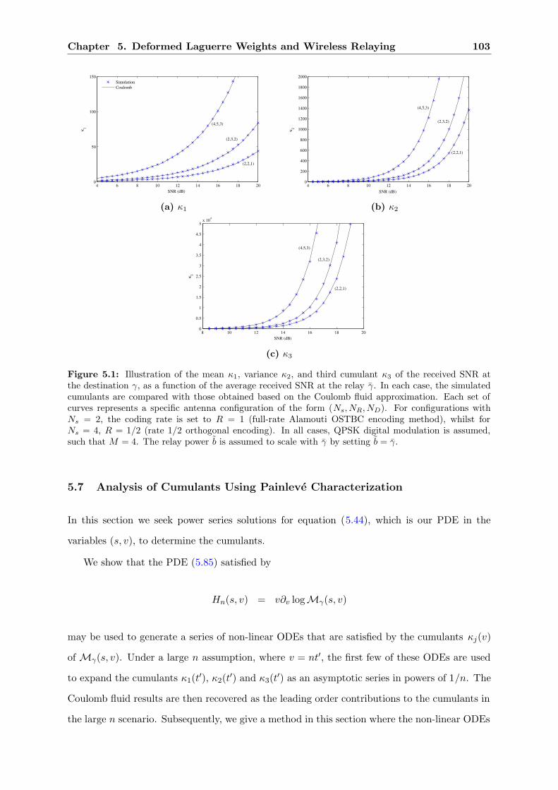
Chapter 5. Deformed Laguerre Weights and Wireless Relaying 103

4 6 8 10 12 14 16 18 200

50

100

150

SNR (dB)

κ 1

SimulationCoulomb

(4,5,3)

(2,3,2)

(2,2,1)

(a) κ1

4 6 8 10 12 14 16 18 200

200

400

600

800

1000

1200

1400

1600

1800

2000

SNR (dB)

κ 2

(2,2,1)

(2,3,2)

(4,5,3)

(b) κ2

8 10 12 14 16 18 200

0.5

1

1.5

2

2.5

3

3.5

4

4.5

5x 10

4

SNR (dB)

κ 3

(2,3,2)

(2,2,1)

(4,5,3)

(c) κ3

Figure 5.1: Illustration of the mean κ1, variance κ2, and third cumulant κ3 of the received SNR atthe destination γ, as a function of the average received SNR at the relay γ. In each case, the simulatedcumulants are compared with those obtained based on the Coulomb fluid approximation. Each set ofcurves represents a specific antenna configuration of the form (Ns, NR, ND). For configurations withNs = 2, the coding rate is set to R = 1 (full-rate Alamouti OSTBC encoding method), whilst forNs = 4, R = 1/2 (rate 1/2 orthogonal encoding). In all cases, QPSK digital modulation is assumed,such that M = 4. The relay power b is assumed to scale with γ by setting b = γ.

5.7 Analysis of Cumulants Using Painleve Characterization

In this section we seek power series solutions for equation (5.44), which is our PDE in the

variables (s, v), to determine the cumulants.

We show that the PDE (5.85) satisfied by

Hn(s, v) = v∂v logMγ(s, v)

may be used to generate a series of non-linear ODEs that are satisfied by the cumulants κj(v)

of Mγ(s, v). Under a large n assumption, where v = nt′, the first few of these ODEs are used

to expand the cumulants κ1(t′), κ2(t′) and κ3(t′) as an asymptotic series in powers of 1/n. The

Coulomb fluid results are then recovered as the leading order contributions to the cumulants in

the large n scenario. Subsequently, we give a method in this section where the non-linear ODEs

5.7 Analysis of Cumulants Using Painleve Characterization 104

generated from the PDE (5.85) are employed systematically to obtain “correction terms” to the

Coulomb fluid results.

We begin by removing the square roots of the PDE and arrive at the following lemma.

Lemma 5.4. Let

K := 2(v(∂vHn) −Hn + n(n+ α)

), (5.83)

and

L := K

[

Hn − 2(1 + cs)2

vc

(∂sHn

)(∂vHn

)−

2(1 + cs)3

(vc)2

(∂sHn

)2

−(2n+Ns + α+ v)∂vHn − 2Ns(1 + cs)vc

∂sHn + (2n−Ns + α)s(1 + cs)

v∂sHn

]

−(1 + cs)2

(vc)2

[(v∂2

vs − ∂s)Hn

][(1 + cs)

(v∂2

vs − ∂s

)Hn + v2c

(∂2

vvHn

)], (5.84)

then the PDE (5.44) may be rewritten in an equivalent square-root-free form, as

4K2Δ∗ 21

(L+ Δ∗ 2

2

)2 =(L2 +K2(Δ∗ 2

1 − Δ∗ 22 ) − Δ∗ 2

1 Δ∗ 22

)2, (5.85)

where Δ∗1 and Δ∗

2 are given by (5.45) and (5.46) respectively.

Now, recall from (5.43) that the function Hn(s, v) is related to the moment generating

function (5.14) through

Hn(s, v) = v∂v logMγ(s, v), (5.86)

where the logarithm of the moment generating function has the expansion,

logMγ(s, v) =∞∑

j=1

(−1)jκj(v)

j!sj , (5.87)

and κj(v) is the jth cumulant. Note that for the sake of brevity we write Mγ(s, v) in place of

Mγ

(v

1+cs , v). Consequently, from (5.86), Hn(s, v) has the following expansion in s,

Hn(s, v) = v

∞∑

j=1

(−1)jcjNs

a′j(v)

j!sj , (5.88)

Chapter 5. Deformed Laguerre Weights and Wireless Relaying 105

where ′ denotes differentiation with respect to v, and aj(v) is related to the jth cumulant κj(v)

by 8

aj(v)cjNs = κj(v). (5.89)

5.7.1 Initial Conditions

Substituting (5.88) into the PDE (5.85)—and assuming that the coefficient of each power of s

in the resulting polynomial expansion in s is zero—gives rise to a system of ODEs satisfied by

the scaled cumulants aj(v). It becomes evident at this point that we require initial conditions

for aj(v), j = 1, 2, . . . , otherwise each cumulant would carry unknown constants of integration.

To find some initial conditions, we recall that the moment generating function in the variables

(s, v) is given by (5.17) (noting the transformations t = v and T = t/(1 + cs)) as

Mγ(s, v) =

(1

1 + cs

)nNs Dn[wAF(∙, s, v)]

Dn[w(α)Lag(∙)]

. (5.90)

Taking logarithms on both sides, and setting v = 0, we have

logMγ(s, 0) = −nNs log(1 + cs). (5.91)

Since by definition, the cumulant generating function is a Taylor expansion near s = 0, with

the cumulants being the coefficients of the Taylor coefficients, we can take the Taylor series

expansion of logMγ(s, 0) near s = 0 as

logMγ(s, 0) = −nNs

∞∑

j=1

(−1)j+1 (cs)j

j. (5.92)

We compare this expression with (5.87), where we have set v = 0:

logMγ(s, 0) =∞∑

j=1

(−1)jcjNsaj(0)j!

sj . (5.93)

Since both (5.92) and (5.93) describe the same moment generating function, its power series

expansion is unique, and hence we may match the coefficients of each power of s. Thus, the

8We introduce aj in order to make a clearer comparison to the Coulomb fluid model and [44] without havingto exactly specify a value for the constant c, since it falls out of the subsequent expansion.

5.7 Analysis of Cumulants Using Painleve Characterization 106

initial conditions for aj(v), j = 1, 2, . . . , 5, at v = 0 are

a1(0) = n, a2(0) = n, a3(0) = 2n, a4(0) = 6n, a5(0) = 24n. (5.94)

5.7.2 Finite n Analysis of κ1

In this subsection, the computation of the mean κ1 is presented. To this end, upon substituting

(5.88) into the PDE (5.85), keeping the lowest power of s in the resulting expansion gives a

highly nonlinear ODE expressed in the factored form

Ψ(1)1 Ψ(1)

2 = 0, (5.95)

where

Ψ(1)1 :=

(a′′1(v)

)2[Ns

2v2

4

(a′′1(v)

)2 + n(n+ α)

(

Ns2(a′1(v)

)2 −Ns2(a′1(v)

)− n(n+ α)

)]

,

(5.96)

and

Ψ(1)2 :=

[

v2(a′′′1 (v)

)+ v

(a′′1(v)

)+ 4n(n+ α)

(

a′1(v) −12

)]2

− (2n+ v + α)2[

v2(a′′1(v)

)2 + 4n(n+ α)(a′1(v)

)(

a′1(v) − 1

)]

. (5.97)

Hence, (5.95) is equivalent to either Ψ(1)1 = 0 or Ψ(1)

2 = 0.

The ODE Ψ(1)1 = 0 has two types of solutions, the first of the form a1(v) = c1v+ c2 where c1

and c2 are constants to be determined. The second is more complicated but can be succinctly

written as

a1(v) = f(c1, Ns, n, α) v sin(2√n√n+ α log v

)+ g(c1, Ns, n, α) v cos

(2√n√n+ α log v

)+ c2 +

v

2,

where c1 and c2 are integration constants, and f and g are algebraic functions in c1, Ns, n and

α (we omit these for brevity).

Whilst these are valid mathematical solutions, it is clear that by taking n large, they differ

drastically from that predicted by the Coulomb fluid method and, for small n, they differ with

the solutions obtained in [44]. This suggests that these are not the solutions of interest to our

problem; thus, we set them aside and henceforth focus on Ψ(1)2 = 0.

Remark 15. From the ODE Ψ(1)2 = 0, the definition a1(v) = κ1(v)/(cNs), and recalling that

c = γ/(RNs), it can be seen that a1(v) is independent of Ns.

Chapter 5. Deformed Laguerre Weights and Wireless Relaying 107

5.7.3 Large n Analysis of κ1

We now examine the equation Ψ(1)2 = 0 in the large n region, which leads to an asymptotic

characterization of a1(v) and thus κ1. To proceed, we scale the variable v by v = nt′. Also,

note that α = n(m/n− 1) ≡ nβ. We find that a1(t′) satisfies the following ODE:

0 =

[t′2

n

(a′′′1 (t′)

)+t′

n

(a′′1(t

′))

+ 2n(1 + β)(2a′1(t

′) − n)]2

−(t′ + 2 + β)2[

t′2 (a′′1(t

′))2 + 4n2(1 + β)

(a′1(t

′)) (a′1(t

′) − n)]

. (5.98)

We assume the first cumulant or κ1 has the following large n expansion

a1(t′) =

κ1(t′)cNs

,

= ne−1(t′) + e0(t

′) +∞∑

k=1

ek(t′)nk

. (5.99)

Substituting the above into (5.98), and setting the coefficients of nj to zero, a system of first

order ODEs for ek(t′) is obtained. These are are solved successively starting from e−1(t′),

followed by e0(t′) and so on.

The expression for a1(0) given by (5.94), gives rise to the initial conditions

e−1(0) = 1 and ek(0) = 0 for k = 0, 1, 2, 3, . . . . (5.100)

As a result e−1(t′) is found to satisfy the ODE

(de−1(t′)dt′

−n

2

)2

=n2(t′ + 2 + β)2

4(t′ + β)2 + 16t′, (5.101)

and has two solutions e−1(t′) = 12

(2 ∓ β + t′ ±

√(t′ + β)2 + 4t′

), both satisfying the initial

condition e1(0) = 1.

We retain the solution that is finite at t′ → ∞

e−1(t′) =

12

(2 + β + t′ −

√(t′ + β)2 + 4t′

), (5.102)

to match with that obtained from the Coulomb fluid computation, namely, (5.78).

5.7 Analysis of Cumulants Using Painleve Characterization 108

Continuing, we set the coefficient of n3 to zero, which implies,

de0dt′

= 0. (5.103)

Setting the coefficient of n2 to zero gives rise to an ODE involving e′

−1(t′), e

′′

−1(t′), e

′′′

−1(t′), e

′

0(t′)

and e′

1(t′) (which we do not state for brevity). Simplifying, with e−1(t′) given by (5.102) and

e′

0(t′) given by (5.103), we find that e1(t′) satisfies:

((t′ + β)2 + 4t′

)7/2

t′(1 + β)de1dt′

= −3t′2 − (β + 2)t′ + 2β2. (5.104)

Setting the coefficient of the next lowest power of n to zero gives rise to an ODE involving

e′

−1(t′), e

′′

−1(t′), e

′′′

−1(t′), e

′

0(t′), e

′′

0(t′), e′′′

0 (t′), e′

1(t′), and e

′

2(t′). From the expression of e−1(t′)

and e′0(t′) given by (5.102) and (5.103) respectively, we find

de2dt′

= 0. (5.105)

Continuing with this process as described above, the next three terms e3(t′), e4(t′) and e5(t′)

are found to satisfy the following equations:

((t′ + β)2 + 4t′

)13/2

t′(1 + β)de3dt′

= l(3)1 (t′), (5.106)

de4dt′

= 0, (5.107)((t′ + β)2 + 4t′

)19/2

t′(1 + β)de5dt′

= l(5)1 (t′), (5.108)

where l(3)1 (t′) and l(5)1 (t′) are given by

l(3)1 (t′) = −40t′6 − 16(β + 2)t′5 + (149β2 − 79β − 79)t′4 + (β + 2)(145β2 − 27β − 27)t′3

−(19β2 − 236β − 236)β2t′2 + 37(β + 2)βt′ − 2β6, (5.109)

l(5)1 (t′) = −1260t′10 + 412 (β + 2) t′9 + 12

(325β2 − 97β − 97

)t′

8

+8(β + 2)(1999β2 − 516β − 516)t′7 −(7967β4 − 70762β3 − 61492β2 + 18540β + 9270

)t′

6

−(β + 2)(23233β4 − 43750β3 − 41500β2 + 4500β + 2250)t′5

−2(4294β4 + 33485β3 + 10575β2 − 45820β − 22910

)β2t′

4

+34(β + 2)(107β2 − 695β − 695)β4t′3 +

(1717β2 + 10072β + 10072

)β6t′

2

−217 (β + 2)β8t′ + 2β10. (5.110)

Chapter 5. Deformed Laguerre Weights and Wireless Relaying 109

Solving ODEs (5.103)–(5.108) with initial conditions ek(0) = 0 for k = 0, 1, 2, . . . , 5, we obtain,

κ1(t′)cNs

=κCF

1 (t′)cNs

+(1 + β)t′2

((t′ + β)2 + 4t′

)5/2

2∑

k=0

A(1)2k+1(t

′)

n2k+1+ O

(1n7

)

, (5.111)

where A(1)1 (t′), A(1)

3 (t′) and A(1)5 (t′) are given by

A(1)1 (t′) = 1, (5.112)

A(1)3 (t′) =

1((t′ + β)2 + 4t′

) +7t′(t′ − 2β − 4)((t′ + β)2 + 4t′

)2 +105t′2(1 + β)

((t′ + β)2 + 4t′

)3 , (5.113)

and

A(1)5 (t′) =

1((t′ + β)2 + 4t′

)2 +2t′(337t′ − 38β − 76)((t′ + β)2 + 4t′

)3 −33t′2(15t′2 + 484t′ + 60t′β − 106β − 106)

((t′ + β)2 + 4t′

)4

2002t′3(6t′2 + 52t′ + 15t′β − 18β − 12)((t′ + β)2 + 4t′

)5 −50050t′4(t′2 + 4t′ + 2t′β − 2β − 1)

((t′ + β)2 + 4t′

)6 . (5.114)

5.7.4 Finite n Analysis of κ2

Having characterized κ1, we now turn to the variance κ2. To this end, equating the coefficients

of the next lowest power of s to zero in the expansion of the PDE (5.85), results in an ODE

which can be factored into the following form

Ψ(1)1

(Ψ(2)

1 + Ψ(2)2 + Ψ(2)

3

)= 0. (5.115)

The ODE Ψ(1)1 = 0, makes a reappearance, which we set aside, leaving the ODE

Ψ(2)1 + Ψ(2)

2 + Ψ(2)3 = 0, (5.116)

where Ψ(2)1 , Ψ(2)

2 and Ψ(2)3 are given by

Ψ(2)1

2Ns= 8v2

(

a1′ −

12

)(v2 (2n− v + α) (a1

′′)2 + (2n+ v + α)n(n+ α)a1′ (a1

′ − 1))a1

′′′

− v4 (2n+ v + α) (a1′′)4 + 2v3 (2n− v + α)

(

a1′ −

12

)

(a1′′)3

− v2

[((2n+ v + α)

((α+ v)(α− v) + 20n(n+ α)

)− 16n(n+ α)(2n+ α)

)(a1

′) (a1′ − 1)

− n (n+ α) (2n− 3v + α)

]

(a1′′)2 + 8 (2n+ v + α)n(n+ α)a1

′ (a1′ − 1)

×

[

v

(

a1′ −

12

)

a1′′ +

((v + α)2 + 4vn

)a1

′(1 − a1′) + n (n+ α)

]

, (5.117)

5.7 Analysis of Cumulants Using Painleve Characterization 110

Ψ(2)2 =

[

2v4 (2n(n+ α) − 1) (a1′′)2 − v3

(va2

′′′

+ 8n(n+ α) (a2′ − 1)

)a1

′′

+ 4v2n(n+ α)

(

v

(

a1′ −

12

)

a2′′ +

((v + α)(2n+ v + α) + 2n(4n+ α− 1)

)(a1

′) (a1′ − 1)

+ n(n+ α) + (a2′ − 1) a1

′ −12a2

′

)]

a1′′′ + 4 v3

(

n(n+ α) −12

)

(a1′′)3 − v4a′′′2 (a′′1)2

+ v2

[

v (2n+ v + α)2 a2′′ − 2

((4(2n+ v + α)2 − 8n(n+ α)

)n(n+ α) − v(2n+ α) − α2

)

a1′

−(12n(n+ α) + 2vn+ (v + α)α

)a2

′ + 4n (n+ α)((2n+ v + α)2 − 2n(n+ α) + 3

)]

(a1′′)2

− 4n(n+ α)v2a′′1

(

a′1 −12

)

(va′′′2 − a′′2) − 12vn2(n+ α)2a′′1 , (5.118)

and

Ψ(2)3

4n(n+ α)= v

[((2n+ v + α)2 + 4n(n+ α) − 2

)(a1

′)2 −((2n+ v + α)2 − 4n(n+ α) +

12

)a2

′

+

((2(2n+ v + α)2 + 1 − 8n(n+ α)

)a2

′ − 3(2n+ v + α)2 + 1 + 4n(n+ α)

)

a1′

]

a1′′

+ v

[(4nv + (v + α)2

)(a1

′) (1 − a′1) + n (n+ α)

]

a2′′ +

(2nv + (v + α)α

)a2

′(1 − a′1)a′1

+

[

2(2n+ v + α)(2n+ α− 2(2n+ v + α)n(n+ α)

)+ 8n(n+ α)

(2n(n+ α) − 1

)]

(a1′)2 (a′1 − 1)

+ 2((2n+ v + α)2 − 4n(n+ α)

)n(n+ α) (a1

′)2 − 2n (n+ α)

(

−12a2

′ + n (n+ α)

)

+ 2(6n(n+ α) − (2n+ v + α)2 − 1

)n (n+ α) a1

′. (5.119)

Clearly, Ψ(2)1 depends on a1(v) only, whilst Ψ(2)

2 and Ψ(2)3 depend on both a1(v) and a2(v).

5.7.5 Large n Analysis of κ2

In computing a large n series expansion for the variance, we proceed in a similar way as was

just done for the mean. First, we replace v by nt′ in (5.116), and then proceed to substitute

the expansion for a1(t′) from (5.111) and

a2(t′) =

κ2(t′)c2Ns

,

= nf−1(t′) + f0(t

′) +∞∑

k=1

fk(t′)nk

, (5.120)

into (5.116).

Chapter 5. Deformed Laguerre Weights and Wireless Relaying 111

Equating the coefficients of nk to zero, a system of first order ODEs for fk(t′) are found.

Comparing with the expression for a2(0) in (5.94) gives rise to the initial conditions

f−1(0) = 1 and fk(0) = 0 for k = 0, 1, 2, 3, . . . . (5.121)

In this case, setting the coefficient of n12 to zero results in a first order ODE for f−1(t′):

df−1

dt′= 1 −

(t′ + β + 2

((t′ + β)2 + 4t′

)1/2 −2(β + 1)t′

((t′ + β)2 + 4t′

)3/2

)

. (5.122)

The solution of this, with the initial condition f−1(0) = 1, reads

f−1(t′) =

(

t′ + 1 +β

2

)

−√

(t′ + β)2 + 4t′

1 −12

β2 + (β + 2)t′((t′ + β)2 + 4t′

)

. (5.123)

Continuing the process, we obtain an ODE for f0(t′):

df0

dt′= −

2Ns(β + 1)t′(t′ − β)(t′ + β)((t′ + β)2 + 4t′

)3 . (5.124)

The solution with the condition f0(0) = 0 reads

f0(t′) =

Ns(1 + β)t′2((t′ + β)2 + 4t′

)2 , (5.125)

from which it can be immediately seen that

nf−1(t′) + f0(t

′) =κCF

2 (t′)c2Ns

,

and we recover κCF2 (t′) found previously.

The ODEs satisfied by fk(t′), k = 1, 2, 3, 4 are reported in Appendix H, equations (H.1)–

(H.4). These will allow us to compute fk(t′) with appropriate initial conditions.

Briefly, the idea is that to determine the ODE satisfied by the kth correction term fk(t′),

for k odd, the preceding 12(k+ 1) ODEs satisfied by fj(t′), j = −1, 1, 3 . . . , k are employed. For

even k, the previous k2 ODEs satisfied by fj(t′), j = 0, 2, 4 . . . , k are employed.

5.7 Analysis of Cumulants Using Painleve Characterization 112

Going through the procedure described, we find that κ2(t′) has the following large n expan-

sion,

κ2(t′)c2Ns

=κCF

2 (t′)c2Ns

+(1 + β)t′2

((t′ + β)2 + 4t′

)5/2

1∑

k=0

A(2)2k+1(t

′)

n2k+1

+Ns(1 + β)t′2

((t′ + β)2 + 4t′

)3

1∑

k=0

B(2)2k+2(t

′)

n2k+2+ O

(1n5

)

, (5.126)

where

A(2)1 (t′) = 3 −

5t′(t′ + 2 + β)((t′ + β)2 + 4t′

) , (5.127)

B(2)2 (t′) = 1 +

7t′(t′ − 2β − 4)((t′ + β)2 + 4t′

) +104t′2(1 + β)

((t′ + β)2 + 4t′

)2 , (5.128)

and A(2)3 (t′) and B(2)

4 (t′) can be found in Appendix I, given by equations (I.4) and (I.5) respec-

tively.

5.7.6 Beyond κ1 and κ2

The same procedure for finding the ODEs satisfied by a1(v) and a2(v) easily extends to higher

cumulants. For the first k cumulants, we can find a system of k coupled non-linear ODEs

satisfied by ai(v), i = 1, 2, . . . , k. Due to the non-linear nature of these ODEs, uncoupling these

would be very difficult.

However, the procedure adopted above for computing the large n expansion series for κ1(t′)

and κ2(t′) can be extended to the higher cumulants much more easily. By way of example, here

we focus on the third cumulant κ3. In this case, an asymptotic expansion for a3(t′) is assumed,

a3(t′) =

κ3(t′)c3Ns

,

= ng−1(t′) + g0(t

′) +∞∑

k=1

gk(t′)nk

, (5.129)

along with the initial conditions,

g−1(0) = 2 and gk(0) = 0 for k = 0, 1, 2, 3, . . . . (5.130)

Chapter 5. Deformed Laguerre Weights and Wireless Relaying 113

For ease of reference, the ODEs satisfied by gk(t′), k = 1, 2, 3, 4, are placed in Appendix H,

equations (H.9)–(H.12).

In this case, we find that the large n expansion of the third cumulant reads

κ3(t′)c3Ns

=κCF

3 (t′)c3Ns

+(1 + β)t′2

((t′ + β)2 + 4t′

)5/2

1∑

k=0

A(3)2k+1(t

′) +N 2s C

(3)2k+1(t

′)

n2k+1

+Ns(1 + β)t′2

((t′ + β)2 + 4t′

)3

1∑

k=0

B(3)2k+2(t

′)

n2k+2+ O

(1n5

)

, (5.131)

where

A(3)1 (t′) = 12 −

10t′(t′ + 4β + 8)((t′ + β)2 + 4t′

) +140t′2(1 + β)

((t′ + β)2 + 4t′

)2 , (5.132)

C(3)1 (t′) =

2t′(t′ − 2β − 4)((t′ + β)2 + 4t′

) +32t′2(1 + β)

((t′ + β)2 + 4t′

)2 , (5.133)

B(3)2 (t′) = 6 +

6t′(37t′ − 19β − 38)((t′ + β)2 + 4t′

) −12t′2(21t′2 + 172t′ + 21t′β − 134β − 134)

((t′ + β)2 + 4t′

)2

+1560t′3(t′2 + 3t′ + t′β − 3β − 2)

((t′ + β)2 + 4t′

)3 , (5.134)

and A(3)3 (t′), C(3)

3 (t′) and B(3)4 (t′) can be found in Appendix I, given by equations (I.10), (I.11)

and (I.12) respectively.

5.7.7 Comparison of Cumulants Obtained from ODEs with those Obtained from Deter-

minant Representation

This subsection serves as a check for consistency of our equations. For small values of n, we

compute the Hankel determinant from the moments formula (5.19), since

Dn(T, t) = det(μj+k(T, t)

)n−1

j,k=0.

Using the transformations (5.41) and (5.42), the moment generating function in s and v reads

Mγ(s, v) =

(1

1 + cs

)nNs det(cj+k(s, v)

)n−1

j,k=0

det(cj+k(0, v)

)n−1

j,k=0

, (5.135)

5.8 SER Performance Measure Analysis Based on Coulomb Fluid 114

where cj(s, v) was derived in [44] as

cj(s, v) := vα+j+1Γ(α+ j + 1)Ns∑

k=0

(Ns

k

)

(cs)k U

(

α+ j + 1, α+ j + 2 − k,v

1 + cs

)

.

(5.136)

For small fixed integer values of n and Ns, e.g., n = 2, 3 and Ns = 10, and n = 4, 5 and Ns = 1,

the above determinant can computed without much difficulty, from which the cumulants follow.

It can be seen that κ1(v)cNs

= a1(v) and κ2(v)c2Ns

= a2(v) obtained from (5.135), satisfied third order

ODEs for a1(v) given by (5.97) and a2(v) given by (5.116). Similar results hold for the higher

cumulants, which provide a consistency check.

5.8 SER Performance Measure Analysis Based on Coulomb Fluid

In this section, and Sections 5.9 and 5.10, we turn our attention to using our exact and Coulomb

fluid characterizations for the moment generating function (5.14) to calculate the symbol error

rate (SER) performance measure, expressed in terms of our moment generating function as

(5.3) or (5.4).

Combining (5.61) with (5.66), (5.69), and (5.70) yields an asymptotic expression for the

moment generating function of the instantaneous SNR. This, in turn, combined with either

(5.3) or (5.4), directly yields analytical approximations for the SER of the MIMO-AF scheme

under consideration. The accuracy of these approximations is confirmed in Fig. 5.2, where they

are compared with simulation results generated by numerically computing the exact SER via

Monte Carlo methods. Different antenna configurations are shown, as represented by the form

(Ns, NR, ND). The curves labeled “Coulomb (Exact SER)” were generated by substituting our

Coulomb fluid approximation into the exact expression of the SER (5.3), whilst the curves la-

beled “Coulomb (Approx SER)” are generated by substituting our Coulomb fluid approximation

into the approximate expression for the SER (5.4).

From these curves, it is remarkable that the Coulomb fluid based approximations, derived

under the assumption of large n, very accurately predict the SER even for small values of n.

This is evident, for example, by examining the set of curves corresponding to the configuration

(2, 3, 2), for which n = 2. In fact, even for the extreme cases with n = 1, the Coulomb fluid

curves still yield quite high accuracy.

Chapter 5. Deformed Laguerre Weights and Wireless Relaying 115

We note that the results in Fig. 5.2 are representative of those presented previously in [44,

Fig. 5]. The key difference therein was that the analytic curves were based on substituting

into either (5.3) or (5.4) an equivalent determinant form of the moment generating function to

that given in (5.18) and (5.19). That representation, involving a determinant of a matrix with

elements comprising sums of Kummer functions, is far more complicated than the Coulomb

fluid representation, which is a simple algebraic equation involving only elementary functions.

The fact that the Coulomb fluid representation yields accurate approximations for the SER for

small as well as large numbers of antennas makes it a useful analytical tool for studying the

performance of arbitrary MIMO-AF systems.

0 5 10 15 20 25

10-4

10-3

10-2

10-1

100

SNR (dB)

SER

Coulomb (Exact SER)Coulomb (Approx SER)Simulation

(2,1,1)

(2,3,2)

(2,2,1)(4,5,3)

(4,6,5)

Figure 5.2: Illustration of the SER versus average received SNR (at relay) γ; comparison of analysisand simulations. As in Fig. 5.1, each set of curves represents a specific antenna configuration of theform (Ns, NR, ND). For configurations with Ns = 2, the coding rate is set to R = 1 (full-rate AlamoutiOSTBC encoding method), whilst for Ns = 4, R = 1/2 (rate 1/2 orthogonal encoding). In all cases,QPSK digital modulation is assumed, such that M = 4. The relay power b is assumed to scale with γby setting b = γ.

5.9 Asymptotic Performance Analysis Based on Coulomb Fluid 116

5.9 Asymptotic Performance Analysis Based on Coulomb Fluid

In this section, we return to the analysis of the moment generating function, and consider the

high SNR scenario where γ → ∞ and b scales in proportion to γ as (see [44])

b := λγ, λ > 0. (5.137)

To this end, we will study the Coulomb fluid based approximation derived in Section 5.5 (to

be complemented in Section 5.10 through analysis based on Painleve equations), where the

variables T ′ and t′ are taken to be dependent on γ, namely,

T ′(s, γ) =t′(γ)

1 + γsRNs

, t′(γ) =1n

(1 + γ)NR

b, (5.138)

Note that as γ → ∞,

t′(γ) −→NR

nλ.

To obtain the desired high SNR expansion, we compute the moment generating function

Mγ as s→ ∞ and γ → ∞. The Coulomb fluid based representation (5.61), when expressed in

terms of T ′(s, γ) and NRnλ reads

Mγ(s) ≈ exp

(

−S2

(T ′(s, γ),

NR

nλ

)− n

[

S1

(T ′(s, γ),

NR

nλ

)−Ns log

(nλT ′(s, γ)

NR

)])

,

(5.139)

where S1 and S2 are given by (5.69) and (5.70) respectively. Our goal is to compute the

expansion of Mγ(s) as s → ∞ and γ → ∞, which turns out to be an expansion in (γs)−1. It

turns out that the cases β = 0 and β 6= 0 behave fundamentally differently, and as such, these

are treated separately.

5.9.1 The Case of β = 0

With β = 0, we have NR = n. An easy computation shows that Mγ admits the following

expansion:

Mγ(s) =∞∑

`=0

A`(γs)d+`/2

, (5.140)

Chapter 5. Deformed Laguerre Weights and Wireless Relaying 117

where A0, A1, A2, A3, . . . are constants independent of s and γ. The leading exponent d is

given by

d = Ns

(

n−Ns

4

)

, (5.141)

whilst the first few A` are

A0 =

(RNs

λ

)Ns(n−Ns/4) (1 +

√1 + 4λ

)2nNs

4Ns(n+Ns/4)(1 + 4λ)Ns2/4

exp

(

−nNs

2λ

[1 −

√1 + 4λ

])

, (5.142)√

λ

RNsA1 = A0

Ns

2

(Ns

√1 + 4λ− 4n

), (5.143)

√λ

RNsA2 =

A1

8

[

2Ns

(Ns

√1 + 4λ− 4n

)−Ns(1 + 4λ) + 8n(2λ− 1)(Ns

√1 + 4λ− 4n

)]

, (5.144)

√λ

RNsA3 =

A2

6

[

Ns

(Ns

√1 + 4λ− 4n

)−

√1 + 4λ

+

[32Nsn

2 − 8n(2Ns2 + 1)(2λ− 1) − 3Ns(1 + 4λ)

]√1 + 4λ

2Ns

(Ns

√1 + 4λ− 4n

)2−Ns(1 + 4λ) − 8n(2λ− 1)

−32n

[Ns

2

4 (1 + 4λ) − 2nNs(2λ− 1) − 3λ+ 14

]

2Ns

(Ns

√1 + 4λ− 4n

)2−Ns(1 + 4λ) − 8n(2λ− 1)

]

. (5.145)

We have refrained from presenting Ak, k ≥ 4, as these are rather long.

Remark 16. For the special case b = γ or λ = 1, implying equal relay and source power, A0

reduces to the remarkably simple formula:

A0 =(RNs)

Ns(n−Ns4 )ϕ2Nsn

20Ns2/4

exp

(Nsn

ϕ

)

, (5.146)

where ϕ = (1 +√

5)/2 is the Golden ratio.

High SNR Analysis of the Symbol Error Rate (SER)

Based on (5.3):

PMPSK =1π

Θ∫

0

Mγ

(gMPSK

sin2 θ

)dθ, Θ =

π(M − 1)M

, gMPSK = sin2( πM

),

the SER of M-PSK modulation can be expanded at high SNR using (5.140), resulting in

PMPSK =1π

∞∑

`=0

A`(γgMPSK)d+`/2

Id,`(Θ), (5.147)

5.9 Asymptotic Performance Analysis Based on Coulomb Fluid 118

where

Id,`(Θ) :=

Θ∫

0

sin2d+` θ dθ. (5.148)

Considering the first order expansion in γ, following [107], we may write

PMPSK =(Gaγ

)−Gd

+ o(γ−Gd

), (5.149)

where we identify

Gd = Ns

(

n−Ns

4

)

, (5.150)

and

Ga = gMPSK

(A0IGd,0(Θ)

π

)− 1Gd, (5.151)

as the so-called diversity order 9 and array gain10 (or coding gain) respectively. We note that

the result for Gd above is consistent with a previous result obtained via a different method

in [98], whilst the expression for Ga appears new.

Whilst it appears that a closed-form solution for the integral (5.148) is not forthcoming

in general (though it can be easily evaluated numerically), such a solution does exist for the

important special case of BPSK modulation, for which M = 2. In this case we have the

particularization, Θ = π/2, for which [56] gives

Id,`(π/2) =√π

2Γ(d+ `/2 + 1/2)Γ(d+ `/2 + 1)

. (5.152)

Hence, using (5.151), Ga admits the simplified form

Ga =

(A0

2√π

Γ(Gd + 1/2)Γ(Gd + 1)

)− 1Gd

. (5.153)

The high SNR results above are illustrated in Fig. 5.3. The “Simulation” curves are based

on numerically evaluating the exact SER relation (5.3); the “Coulomb fluid (Exact)” curves

are based on substituting (5.139) into (5.3) and numerically evaluating the resulting integral;

the “Coulomb fluid (Leading term only)” curves are based on (5.149); whilst “Coulomb fluid

9This is the number of replicas of a signal that can can be sent across the MIMO channel. An increasingnumber of identical signals improves the quality and reliability of reception.

10Denotes the improvement in received SNR that results from combining multiple copies of the same signal atthe destination terminal.

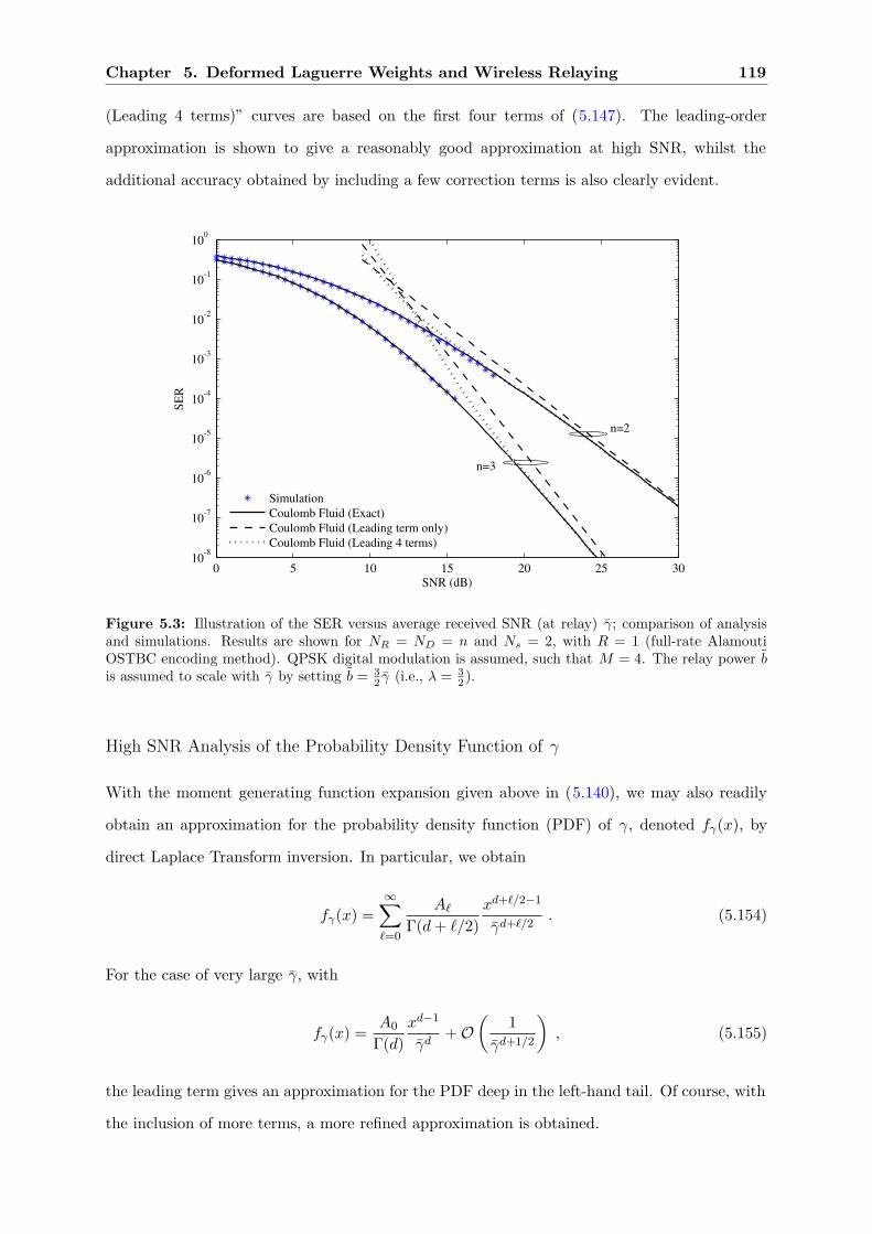
Chapter 5. Deformed Laguerre Weights and Wireless Relaying 119

(Leading 4 terms)” curves are based on the first four terms of (5.147). The leading-order

approximation is shown to give a reasonably good approximation at high SNR, whilst the

additional accuracy obtained by including a few correction terms is also clearly evident.

0 5 10 15 20 25 3010

-8

10-7

10-6

10-5

10-4

10-3

10-2

10-1

100

SNR (dB)

SER

SimulationCoulomb Fluid (Exact)Coulomb Fluid (Leading term only)Coulomb Fluid (Leading 4 terms)

n=3

n=2

Figure 5.3: Illustration of the SER versus average received SNR (at relay) γ; comparison of analysisand simulations. Results are shown for NR = ND = n and Ns = 2, with R = 1 (full-rate AlamoutiOSTBC encoding method). QPSK digital modulation is assumed, such that M = 4. The relay power bis assumed to scale with γ by setting b = 3

2 γ (i.e., λ = 32 ).

High SNR Analysis of the Probability Density Function of γ

With the moment generating function expansion given above in (5.140), we may also readily

obtain an approximation for the probability density function (PDF) of γ, denoted fγ(x), by

direct Laplace Transform inversion. In particular, we obtain

fγ(x) =∞∑

`=0

A`Γ(d+ `/2)

xd+`/2−1

γd+`/2. (5.154)

For the case of very large γ, with

fγ(x) =A0

Γ(d)xd−1

γd+ O

(1

γd+1/2

)

, (5.155)

the leading term gives an approximation for the PDF deep in the left-hand tail. Of course, with

the inclusion of more terms, a more refined approximation is obtained.

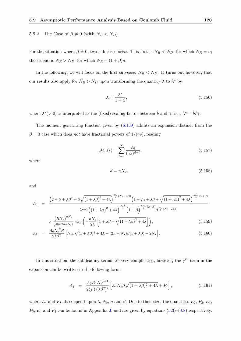
5.9 Asymptotic Performance Analysis Based on Coulomb Fluid 120

5.9.2 The Case of β 6= 0 (with NR < ND)

For the situation where β 6= 0, two sub-cases arise. This first is NR < ND, for which NR = n;

the second is NR > ND, for which NR = (1 + β)n.

In the following, we will focus on the first sub-case, NR < ND. It turns out however, that

our results also apply for NR > ND upon transforming the quantity λ to λ∗ by

λ =λ∗

1 + β, (5.156)

where λ∗(> 0) is interpreted as the (fixed) scaling factor between b and γ, i.e., λ∗ = b/γ.

The moment generating function given by (5.139) admits an expansion distinct from the

β = 0 case which does not have fractional powers of 1/(γs), reading

Mγ(s) =∞∑

`=0

A`(γs)d+`

, (5.157)

where

d = nNs, (5.158)

and

A0 =

(2 + β + λβ2 + β

√(1 + λβ

)2+ 4λ

)Ns2 (Ns−nβ)(

1 + 2λ+ λβ +√(

1 + λβ)2

+ 4λ)nNs

2 (2+β)

λnNs

((1 + λβ

)2+ 4λ

)Ns2

4(1 + β

)nNs2 (2+β)

βNs2 (Ns−2nβ)

×

(RNs

)nNs

2Ns2 (2n+Ns)

exp

(

−nNs

2λ

[

1 + λβ −√(

1 + λβ)2

+ 4λ

])

, (5.159)

A1 =A0Ns

2R

2λβ2

[Nsβ

√(1 + λβ)2 + 4λ− (2n+Ns)β(1 + λβ) − 2Ns

]. (5.160)

In this situation, the sub-leading terms are very complicated, however, the jth term in the

expansion can be written in the following form:

Aj =A0R

jNsj+1

2(j!) (λβ2)j

[EjNsβ

√(1 + λβ)2 + 4λ+ Fj

], (5.161)

where Ej and Fj also depend upon λ, Ns, n and β. Due to their size, the quantities E2, F2, E3,

F3, E4 and F4 can be found in Appendix J, and are given by equations (J.3)–(J.8) respectively.

Chapter 5. Deformed Laguerre Weights and Wireless Relaying 121

High SNR Analysis of the Symbol Error Rate (SER)

Based on (5.3), the SER of MPSK modulation can be expanded at high SNR using (5.157) into

PMPSK =1π

∞∑

`=0

A`(γgMPSK)d+`

Id+`(Θ), (5.162)

where

Ir(Θ) :=∫ Θ

0sin2r θ dθ . (5.163)

Note that here, in contrast to (5.148), the exponent r is a positive integer. As such, (5.163)

admits the following closed-form solution: [56, Eq. (2.513.1)]

Ir(Θ) =Θ22r

(2rr

)

+(−1)r

22r−1

r−1∑

j=0

(−1)j(

2rj

) sin(2(r − j)Θ

)

2(r − j). (5.164)

As before, a first-order approximation is of key interest, giving

PMPSK =(Gaγ

)−Gd

+ o(γ−Gd

), (5.165)

where we identify the diversity order

Gd = nNs, (5.166)

and the array gain

Ga = gMPSK

(A0IGd

(Θ)π

)− 1Gd

. (5.167)

The result for Gd above is consistent with a result obtained via a different method in [98],

whilst the expression for Ga appears new. The high SNR results above, for the case β 6= 0, are

illustrated in Fig. 5.4. As before, the “Simulation” curves are based on numerically evaluating

the exact SER relation (5.3), and the “Coulomb fluid (Exact)” curves are based on substituting

(5.139) into (5.3) and numerically evaluating the resulting integral. Moreover, the “Coulomb

fluid (Leading term only)” curves are based on (5.165), whilst the “Coulomb fluid (Leading 5

terms)” curves are based on the first five terms of (5.162). Again, the leading-order approxi-

mation is shown to give a reasonably good approximation at high SNR, whilst the additional

accuracy obtained by including a few correction terms is also evident.

5.9 Asymptotic Performance Analysis Based on Coulomb Fluid 122

5 10 15 20 2510

-8

10-6

10-4

10-2

100

SNR (dB)

SER

SimulationCoulomb Fluid (Exact)Coulomb Fluid (Leading term only)Coulomb Fluid (Leading 5 terms)

ND

=6 ND

=3

Figure 5.4: Illustration of the SER versus average received SNR (at relay) γ; comparison of analysisand simulations. Results are shown for NR = Ns = 2, with R = 1 (full-rate Alamouti OSTBC encoding).QPSK digital modulation is assumed, such that M = 4. The relay power b is assumed to scale with γby setting b = 3

2 γ (i.e., λ = 32 ).

High SNR Analysis of the Probability Density Function of γ

As before, based on the moment generating function expansion (5.157), applying for β 6= 0, we

can immediately take a Laplace inversion to obtain the following high SNR representation for

the PDF of γ,

fγ(x) =∞∑

`=0

A`Γ(d+ `)

xd+`−1

γd+`. (5.168)

We are mainly interested in the leading order term, and so we write the above as

fγ(x) =A0

Γ(d)xd−1

γd+ O

(1

γd+1

)

. (5.169)

Note that despite the similarity with (5.155), interestingly, these results do not coincide upon

taking β → 0 in (5.169), due to the differences in d and A0. This seems to indicate that the

double asymptotics γ → ∞ and β → 0 are non-commutative, i.e.

limγ→∞

limβ→0

Mγ(s) 6= limβ→0

limγ→∞

Mγ(s). (5.170)

Chapter 5. Deformed Laguerre Weights and Wireless Relaying 123

5.10 Characterizing A0 Through Painleve V

In this section, we obtain the leading term of the large s and large γ expansion (5.157) from

a Painleve V differential equation, thus demonstrating the accuracy of the Coulomb fluid ap-

proximation. We will focus in this section on the case β 6= 0.

Recall that the moment generating function of SNR γ, regarded a function of s and t, given

by (5.14), reads,

Mγ(s, t) =1

Kn,α

(1

1 + cs

)nNs 1n!

∫

[0,∞)n

∏

1≤j<k≤n

(xj − xk)2

n∏

`=1

xα` e−x`

(t+ x`t

1+cs + x`

)Ns

dx`,

(5.171)

where Kn,α is a normalization constant, given by (5.21). We also recall that c and t are given

by

c =γ

RNs, t =

(1 + γ)NR

b, where b := λγ, (5.172)

respectively. So as γ → ∞, we note that t→ NR/λ.

A simple computation shows that Mγ(s, t) admits the following expansion for large γs:

Mγ(s, t) =(RNs)nNs

Kn,α(γs)nNs

(

1 −nNs

γs+ . . .

)

×1n!

∫

[0,∞)n

∏

1≤j<k≤n

(xj − xk)2n∏

`=1

xα−Ns

` e−x` (t+ x`)Ns

(

1 −tRN2

s

γsx`+ . . .

)

dx`,

=(RNs)nNs

Dn[wdLag(∙, 0, α−Ns, Ns)]1

(γs)nNsDn

[wdLag(∙, t, α−Ns, Ns)

]

−RnNs+1NnNs+2

s

Dn[wdLag(∙, 0, α−Ns, Ns)]1

(γs)nNs+1

[

nDn

[wdLag(∙, t, α−Ns, Ns)

]

+t

n!

∫

[0,∞)n

∏

1≤j<k≤n

(xj − xk)2(

n∑

i=1

x−1i

)n∏

`=1

xα−Ns

` e−x` (t+ x`)Ns dx`

]

+ O

(1

(γs)nNs+2

)

, (5.173)

where wdLag(x, t, α−Ns, Ns) is the deformation of the classical Laguerre weight, i.e.,

wdLag(x, t, α−Ns, Ns) = xα−Nse−x(t+ x)Ns , t > 0, α−Ns > −1, (5.174)

and Kn,α = Dn[wdLag(∙, 0, α−Ns, Ns)] is independent of t.

5.10 Characterizing A0 Through Painleve V 124

The condition α − Ns > −1 is required for the validity of the orthogonality relation with

respect to the generalized Laguerre weight w(α−Ns)Lag (x) (see [100]). This, in turn, will ensure the

validity of the first two terms in (5.173), while for the multiple integral in the third term to

converge, the condition α−Ns > 0 is required.

For the problem at hand, α and Ns are integers, satisfying α ≥ 0 and Ns > 0. Therefore

α ≥ Ns implies that the result for A0 presented below is valid for α > 0.

Comparing the expansion (5.173) with (5.157), we see that the diversity order is

d = nNs, (5.175)

and

A0 = (RNs)nNs

Dn[wdLag(∙, t, α−Ns, Ns)]Dn[wdLag(∙, 0, α−Ns, Ns)]

. (5.176)

We see that A0 is up to a constant the Hankel determinant which generates a particular

Painleve V and shows up in the single-user MIMO problem studied in [29].

We obtain A0, through a large n expansion of

Dn[wdLag(∙, t, α−Ns, Ns)]Dn[wdLag(∙, 0, α−Ns, Ns)]

,

for α > 0. We will see that A0 precisely matches that obtained in (5.159).

From [29] we learned that the logarithmic derivative of Dn[wdLag(∙, t, α − Ns, Ns)] with

respect to t,

Hn(t) := td

dtlogDn[wdLag(∙, t, α−Ns, Ns)],

= td

dtlog

(Dn[wdLag(∙, t, α−Ns, Ns)]Dn[wdLag(∙, 0, α−Ns, Ns)]

)

, (5.177)

satisfies the Painleve V:

(tH ′′

n

)2=

[(t+ 2n+ α

)H ′n −Hn + nNs

]2

−4(tH ′

n −Hn + n(n+ α))(H ′n

)(H ′n +Ns

), (5.178)

where ′ denotes derivative w.r.t. t.

Chapter 5. Deformed Laguerre Weights and Wireless Relaying 125

We restrict to the case where NR < ND, for which NR = n. The case where NR > ND can

be considered in a similar fashion as outlined in Section 5.9.2. Setting α = nβ in the above

equation, where β = mn − 1 is a fixed positive number, and with the change of variable

t =n

λ, (5.179)

an easy computation shows that Yn(λ) := Hn(n/λ) satisfies

λ4

n2

(2Y ′

n + λY ′′n

)2=

[

λ((β + 2)λ+ 1

)Y ′n + Yn − nNs

]2

+4λ2

n2

(− λY ′

n − Yn + (1 + β)n2)(Y ′n

)(− λ2Y ′

n + nNs

), (5.180)

where ′ denotes derivative with respect to λ.

We seek a solution for Yn(λ) in the form

Yn(λ) = np−1(λ) + p0(λ) +∞∑

j=1

pj(λ)nj

, (5.181)

from which A0(λ) is found to be

A0(λ) = (RNs)nNs exp

−

λ∫

∞

np−1(λ′) + p0(λ′) +∑∞

j=1 n−jpj(λ′)

λ′dλ′

, (5.182)

≈ (RNs)nNs exp

−

λ∫

∞

np−1(λ′) + p0(λ′)λ′

dλ′

[

1 −1n

λ∫

∞

p1(λ′)λ′

dλ′ + O

(1n2

)]

.

(5.183)

Substituting (5.181) into (5.180) leads to (5.180) taking the form

c−2n2 + c−1n+ c0 +

∞∑

j=1

cjn−j = 0, (5.184)

where c−2 depends on p−1(λ) and its derivatives, and ci, i = −1, 0, 1, 2, . . . , depend on p−1(λ),

p0(λ) up to pi+1(λ) and their derivatives. Of course, each ci also depends upon λ, Ns and β.

Assuming that the coefficient of nk is zero, we find that the equation c−2 = 0 gives us

[

λ((β + 2)λ+ 1

)p′−1(λ) + p−1(λ) −Ns

]2

= 4λ2(1 + β)p′−1(λ)(λ2p′−1(λ) +Ns

). (5.185)

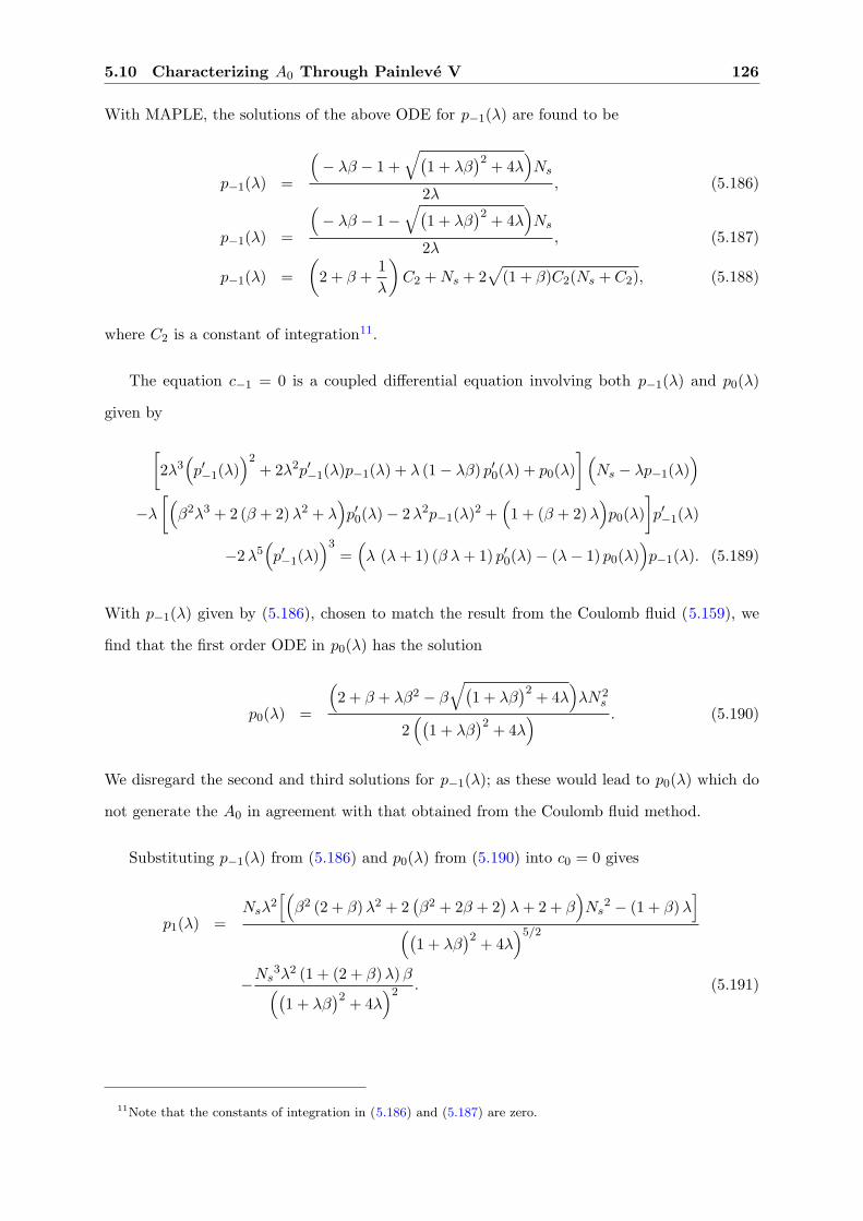
5.10 Characterizing A0 Through Painleve V 126

With MAPLE, the solutions of the above ODE for p−1(λ) are found to be

p−1(λ) =

(− λβ − 1 +

√(1 + λβ

)2 + 4λ)Ns

2λ, (5.186)

p−1(λ) =

(− λβ − 1 −

√(1 + λβ

)2 + 4λ)Ns

2λ, (5.187)

p−1(λ) =

(

2 + β +1λ

)

C2 +Ns + 2√

(1 + β)C2(Ns + C2), (5.188)

where C2 is a constant of integration11.

The equation c−1 = 0 is a coupled differential equation involving both p−1(λ) and p0(λ)

given by

[

2λ3(p′−1(λ)

)2+ 2λ2p′−1(λ)p−1(λ) + λ (1 − λβ) p′0(λ) + p0(λ)

](Ns − λp−1(λ)

)

−λ

[(β2λ3 + 2 (β + 2)λ2 + λ

)p′0(λ) − 2λ2p−1(λ)2 +

(1 + (β + 2)λ

)p0(λ)

]

p′−1(λ)

−2λ5(p′−1(λ)

)3=(λ (λ+ 1) (β λ+ 1) p′0(λ) − (λ− 1) p0(λ)

)p−1(λ). (5.189)

With p−1(λ) given by (5.186), chosen to match the result from the Coulomb fluid (5.159), we

find that the first order ODE in p0(λ) has the solution

p0(λ) =

(2 + β + λβ2 − β

√(1 + λβ

)2 + 4λ)λN2

s

2((

1 + λβ)2 + 4λ

) . (5.190)

We disregard the second and third solutions for p−1(λ); as these would lead to p0(λ) which do

not generate the A0 in agreement with that obtained from the Coulomb fluid method.

Substituting p−1(λ) from (5.186) and p0(λ) from (5.190) into c0 = 0 gives

p1(λ) =Nsλ

2[(β2 (2 + β)λ2 + 2

(β2 + 2β + 2

)λ+ 2 + β

)Ns

2 − (1 + β)λ]

((1 + λβ

)2 + 4λ)5/2

−Ns

3λ2 (1 + (2 + β)λ)β((

1 + λβ)2 + 4λ

)2 . (5.191)

11Note that the constants of integration in (5.186) and (5.187) are zero.

Chapter 5. Deformed Laguerre Weights and Wireless Relaying 127

Hence, A0(λ) has a large n expansion

A0(λ) = q0(λ)

[

1 +q1(λ)n

+ O

(1n2

)]

, (5.192)

where

q0(λ) =

(2 + β + λβ2 + β

√(1 + λβ

)2+ 4λ

)Ns2 (Ns−nβ)(

1 + 2λ+ λβ +√(

1 + λβ)2

+ 4λ)nNs

2 (2+β)

λnNs

((1 + λβ

)2+ 4λ

)Ns24(1 + β

)nNs2 (2+β)

βNs2 (Ns−2nβ)

×

(RNs

)nNs

2Ns2 (2n+Ns)

exp

(

−nNs

2λ

(1 + λβ −

√(1 + λβ

)2+ 4λ

))

. (5.193)

The leading term of A0 in (5.192) agrees precisely with the A0 computed via the Coulomb

fluid method in (5.159).

Using a method similar to the cumulant analysis of Section 5.7, we can also compute the

first correction term to A0 (i.e., the quantity q1(λ)) using (5.191), which reads

q1(λ) =Ns

( (2Ns

2 − 1)β2 + 2

(8Ns

2 − 1)(1 + β)

)

24(1 + β)

[1β−

λ2(β2λ+ 3β + 6)((

1 + λβ)2

+ 4λ)3/2

]

−(2β λ+ 4λ+ 1)Ns

3

2β((

1 + λβ)2

+ 4λ) −

(2 + β)(2Ns

2 − 1)Ns

8((

1 + λβ)2

+ 4λ)3/2

(1 + β)

[

(2 + β)λ+13

]

+(2 + β)N3

s λ2

((1 + λβ

)2+ 4λ

)3/2. (5.194)

Higher order corrections could also be obtained in a similar way.

5.11 Summary of Chapter

In this chapter, we have studied the Hankel determinant that is generated from a weight function

of the form

wAF(x, T, t) = xαe−x(t+ x

T + x

)Ns

, x ∈ [0,∞), α > −1, T, t,Ns > 0,

which is a “two-time” deformation of the classical Laguerre weight, xαe−x.

This Hankel determinant is related to the moment generating function, Mγ(s), of the signal-

to-noise ratio of a multiple-input multiple-output (MIMO) antenna wireless communication

system with Ampify-and-Forward relaying.

5.11 Summary of Chapter 128

The main results of this chapter are:

• In Section 5.3, we derive a PDE (Theorem 5.1) satisfied by the Hankel determinant

Dn[wAF(∙, T, t)] using the ladder operator approach—for finite n. This PDE has re-

ductions to the Painleve V under various limits, and may be considered its ‘two-time’

generalization.

• In Section 5.4, we investigated several asymptotic limits of Dn. In particular, the ladder

operator approach allowed us to establish finite n ODEs and PDEs satisfied by Dn in the

cases where T → ∞ and t→ ∞, and Ns → ∞ (Theorem 5.2) respectively.

• In Section 5.5, we used the Coulomb fluid method (see Chapter 3) to compute an asymp-

totic (large n) approximation for the Hankel determinant Dn, and thus a corresponding

approximation for Mγ(s).

• In Section 5.6, we employed our Coulomb fluid results to compute expressions for the

cumulants κi of the received SNR γ. Subsequently, in Section 5.7, we used the PDE

from Theorem 5.1 to obtain a system of coupled ODEs satisfied by the cumulants (having

been suitably scaled). From these ODEs, we calculated an asymptotic expansion for the

first three cumulants in powers of 1/n, where our analysis can easily extend to higher

cumulants. The Coulomb fluid results from Section 5.6 were recovered as the leading

order contributions to the asymptotic expansion of the cumulants.

• In Section 5.8, we turned our attention to using our exact and Coulomb fluid results for

Mγ(s) to calculate the error performance of MIMO-AF systems, in particular the symbol

error rate (SER).

• Both the Painleve and Coulomb fluid characterizations were shown to yield extremely

accurate approximations for the cumulants and error performance of MIMO-AF systems,

even small values of n.

• In Section 5.9, we used the Coulomb fluid results to obtain an asymptotic expansion

for Mγ(s) in powers of 1/(γs), valid for scenarios for which the average received SNR

is high. From this, we derived key quantities of interest to communication engineers,

including the so-called diversity order and array gain. These results revealed fundamental

differences between the scenarios NR = ND (β = 0) and NR 6= ND (β 6= 0). Subsequently

in Section 5.10, the Coulomb fluid results for the diversity order and array gain were

recovered for β > 0 using a power series solution of the Painleve V differential equation,

validating our approach.

129

Chapter 6

Summary

In this chapter, we discuss the results that have been presented in this thesis and describe how

future work can be done related to each chapter.

In this thesis, we have considered the sequence of orthogonal polynomials and the Han-

kel determinant associated with two different weight functions w(x), supported on an interval

[A,B] ⊆ R. Our main tool is the systematic application of the compatibility conditions (S1),

(S2) and (S′2), obtained from the ladder operators satisfied by the orthogonal polynomials. The

key idea behind using the compatibility conditions is to express the recurrence coefficients αn

and βn, the Hankel determinant Dn[w]; and their derivatives (with respect to some parameter) in

terms of auxiliary variables Rn, rn, R∗n and r∗n. We can then find differential equations satisfied

by the auxiliary variables; or by eliminating our auxiliary variables, we can find differential-

difference identities satisfied by our recurrence coefficients, and differential identities satisfied

by Dn[w].

Also, in the limit n → ∞, we used the Coulomb fluid linear statistics formulae (which are

based on singular integral equations) found in [23, 27] to find the leading order asymptotics of

Dn[w].

6.1 Discussion of Chapter 4

In Chapter 4 we considered the weight function:

w(x, k2) = (1 − x2)α(1 − k2x2)β , x ∈ [−1, 1], α > −1, β ∈ R, k2 ∈ (0, 1).

6.1 Discussion of Chapter 4 130

For this weight, the special case of α = β = −12 was originally studied by Rees in [90].

Through the application of the ladder operator formalism, we generalized (valid for α > −1 and

β ∈ R) two of Rees’ results, found in [90]. First, we found a second-order linear ODE satisfied by

the orthogonal polynomials corresponding to w(x, k2). Second, we found a recurrence relation

satisfied by both βn andn−1∑

j=0βj = p1(n).

We found two second-order non-linear recurrence relations, one satisfied by βn, and one

by p1(n). We also found a third-order non-linear recurrence relation satisfied by βn, derived

independently from the second-order relation. We verified that for special values of α, β and

k2, both recurrence relations for βn have solutions which agree with existing results. The link

between both recurrence relations is still unresolved, i.e. no first integral has been identified

which reduces the third-order equation into the second-order equation.

With the difference equations at our disposal, we used them to compute the complete asymp-

totic expansions for βn and p1(n) in powers of 1/n. To demonstrate the versatility of our ap-

proach, we combined the large n expansion of p1(n) with Toda-type time-evolution equations

satisfied by the Hankel determinant (treating k2 as the differentiation variable). Using this

method, we calculated the complete large n expansion for Dn[w(∙, k2)]. As a validation of our

method, we can check that that the leading order term of the expansion agree with known

results obtained using the Coulomb fluid [6] and Riemann-Hilbert [38, 69] approaches.

Finally, through a change of variable, we expressed the logarithmic derivative of the Hankel

determinant as the sum of two functions—which we later identified as the coefficients p1(2n)

and p1(2n+ 1) for the case where n is even, and p1(2n+ 1) and p1(2n+ 2) for the case where

n is odd—each of which are related to different special cases of the σ-form of the Painleve VI

differential equation.

Since we have a second order difference equation satisfied by p1(n− 1), p1(n) and p1(n+1),

a natural progression would be to find a discrete analog of the σ-form. Namely, a second-order

equation in n satisfied by each σ-function for fixed k2. For convenience, let p1(2n) := f(n) and

p1(2n+ 1) := g(n), where f(n) and g(n) are related to Painleve VI σ-functions (for a different

choice of parameter). Letting n → 2n and n → 2n + 1 in the difference equation satisfied by

p1(n) , we obtain one equation satisfied by f(n+1), f(n) and g(n), and a second by g(n), f(n)

and g(n− 1). This can be regarded as first order non-linear recurrence system satisfied by both

σ-forms. Due to the non-linearity of these equations, de-coupling these equations may prove to

be difficult.

Chapter 6. Summary 131

6.2 Discussion of Chapter 5

In Chapter 5, we considered the received SNR distribution of a certain MIMO communication

system adopting AF relaying. We showed that the mathematical problem of interest pertains to

computing a certain Hankel determinant generated by a two-time deformation of the classical

Laguerre weight

wAF(x, T, t) = xαe−x(t+ x

T + x

)Ns

, x ∈ [0,∞), α > −1, T, t,Ns > 0.

By employing the ladder operator approach—for finite n—together with Toda-type evolution

equations in the ‘time’ variables T and t, we found a second order partial differential equation

satisfied by the logarithmic derivative of the Hankel determinant, which reduces to a Painleve V

under various limits. This result yields an exact and fundamental characterization of the SNR

distribution, through its moment generating function.

It is important to note here that if we had analyzed the original moment generating function

(5.7), as found in [44], we would have considered the weight

w(x, s) = xαe−x(

t+ xt

1+cs + x

)Ns

, x ∈ [0,∞),

where t, α, c and Ns are constants. Using the ladder operator approach, we would have

found that we did not possess enough equations to find a differential equation in s satisfied

by Dn[w(∙, s)]. By introducing a second independent variable t, we gain extra Toda-type time-

evolution equations in t, which we can take advantage of to find a PDE satisfied by Dn[w(∙, s, t)],

or equivalently Dn[w(∙, T, t)].

Complementary to the exact representation, we also introduced the linear statistics Coulomb

fluid approach as an efficient way to compute very quickly the asymptotic properties of the

moment generating function for sufficiently large dimensions (i.e., for sufficiently large numbers

of antennae, n). These results, which have only started to be used recently in problems related to

wireless communications and information theory, produced an approximation for the moment

generating function in terms of simple elementary functions. These were employed to yield

simple approximations for the error probability (for a class of M -PSK digital modulation),

which were shown via simulations to be remarkably accurate, even for very small dimensions

(small values for n).

6.3 Final Remarks 132

To further demonstrate the utility of our two methodologies, we employed our asymptotic

Coulomb fluid characterization in conjunction with the PDE representation to provide a rigorous

study of the cumulants of the SNR distribution. Combining the PDE and Coulomb fluid

representation, we computed the asymptotic expansion of the first few cumulants in powers of

1/n; a procedure which readily extends to higher cumulants.

We also derived asymptotic properties of the moment generating function when the aver-

age SNR was sufficiently high, and in such regime—using the Coulomb fluid approach and a

Painleve V equation—extracted key performance quantities of engineering interest, namely, the

array gain and diversity order. It was seen that there exists fundamental differences between the

cases β = 0 and β 6= 0. However, this difference was not seen in the analysis of the cumulants

of the received SNR γ, since the analytical results for the cumulants are valid for β ≥ 0. This

is due to the non-commutative limits s → ∞ and β → 0 of the moment generating function; a

phenomenon ideal for further consideration.

A problem for future consideration would be to use the PDE representation of the moment

generating function to recover the results of Section 5.9. The Coulomb fluid approach is crucial

here since it readily allows us to calculate the asymptotic expansion of the moment generating

in the high SNR scenario. However, in attempting to use the PDE (in the variables s and λ),

by combining

Hn(s, λ) = −λ∂

∂λlogMγ(s, λ), and Mγ(s, λ) ∼

A0(λ)sd

, as s→ ∞,

it can be seen that the diversity order d vanishes. To recover A0(λ), various limits will have

to be taken in the PDE, including n → ∞, s → ∞, γ → ∞ and optionally β → 0. A further

problem would be to recover the result for A0(λ) from Section 5.10 for β = 0, since in this case,

the multiple integral representation of A0(λ) is divergent and the diversity order disagrees with

our Coulomb fluid result.

6.3 Final Remarks

As we have shown, the ladder operator approach allows us to characterize the orthogonal poly-

nomials and Hankel determinant associated with each weight we have studied in an algorithmic

manner. This in turn, eventually leads us to obtain closed-form second-order ODE/PDEs sat-

isfied by logarithmic derivative of the Hankel determinant. In the case where n is large, the

Chapter 6. Summary 133

Coulomb fluid method gives us a leading order approximation of the Hankel determinant in

terms of elementary functions, which we obtain from solving singular integrals.

We can use these two approaches to study more complicated weight functions. The key with

the ladder operator approach seems to be introducing sufficient number of ‘time’ parameters (as

done in Chapter 5) within the weight function in order to generate a extra Toda-type equations

satisfied by hn, αn, βn, p1(n) andDn[w] (which are expressed in terms of our auxiliary variables).

As a further example, in a problem related to the study of quantum semiconductors, the

moment generating function of the noise distribution due to quantum effects (known as shot-

noise) was expressed in [19] in terms of a Hankel determinant generated by a special case of the

deformed shifted Jacobi weight:

w(x, t) = e−tx(1−x)xα, x ∈ [0, 1], α > −1, t ∈ R.

In this case, the Toda-type equations obtained for αn, βn and p1(n) would be quite complicated,

and would be quite difficult to manipulate (we would in fact obtain a combined form of the first

and second Lattice equations of the Toda hierarchy [61, 97]).

A better approach would be to consider the weight function

w(x, t, s) = e−tx+sx2xα(1 − x)β , x ∈ [0, 1], α, β > −1, t, s ∈ R.

The shot-noise generating function can then be studied by setting β = 0 and s = t. A weight

of this form has been recently studied in [86] using τ -function theory, from which a fourth-

order PDE satisfied by the Hankel determinant was obtained. Applying the ladder operator

approach, we simply state here that we can directly obtain a second-order PDE satisfied by

2s∂t logDn(s, t) (third-order PDE in Dn(s, t) overall).

134

Appendix A

Painleve Equations

This appendix provides a brief background on the Painleve differential equations and their

associated σ-forms, since they appear several times throughout Chapters 4 and 5. Much of this

material can be found in [33, 57, 63, 85].

The Painleve equations were derived between 1895–1910 by Painleve, Gambier and Fuchs

while studying the following problem:

Given a second order ordinary differential equation of the form

w′′(t) = R(t, w(t), w′(t)

), (A.1)

where R(t, w(t), w′(t)

)is a rational function in w(t) and w′(t) and analytic in t. How many

possible ODEs of the form (A.1) exist with the property that the only movable singularities

(singularities which depend on the constants of integration) of solutions to (A.1) are poles?

Differential equations with solutions possessing this property are said to possess the Painleve

property, or are of Painleve type.

Painleve [88] and Gambier [54] proved that there exists 50 canonical ODEs of the form (A.1)

which satisfy the Painleve property, and are referred to as equations of Painleve type. Further,

of these 50 equations, 44 are solvable in terms of either elliptic functions, solutions to second or

third order linear ODEs, or solutions of the following six non-linear ODEs:

w′′(t) = 6(w(t)

)2 + t, (PI)

w′′(t) = 2(w(t)

)3 + tw(t) + α, (PII)

w′′(t) =

(w′(t)

)2

w(t)−w′(t)t

+α(w(t)

)2 + β

t+ γ(w(t)

)3 +δ

w(t), (PIII)

Appendix A. Painleve Equations 135

w′′(t) =

(w′(t)

)2

2w(t)+

32

(w(t)

)3 + 4t(w(t)

)2 + 2(t2 − α)w(t) +β

w(t), (PIV)

w′′(t) =

(1

2w(t)+

1w(t) − 1

)(w′(t)

)2 −w′(t)t

+(w(t) − 1)2

t2

(

αw(t) +β

w(t)

)

+γw(t)t

+δw(t)

(w(t) + 1

)

w(t) − 1, (PV)

w′′(t) =12

(1

w(t)+

1w(t) − 1

+1

w(t) − t

)(w′(t)

)2 −

(1t

+1

t− 1+

1w(t) − t

)

w′(t)

+w(t)

(w(t) − 1

)(w(t) − t

)

t2(t− 1)2

(

α+βt

w(t)+

γ(t− 1)(w(t) − 1

)2 +δt(t− 1)(w(t) − t

)2

)

, (PVI)

where ′ denotes differentiation with respect to t and α, β, γ and δ are arbitrary constants.

Each Painleve equation PI-PVI is related to its σ-form through a Hamiltonian system [85].

A.1 Hamiltonian Structure

Okamoto [83–85] showed that each Painleve equation PI–PVI can be written as the following

Hamiltonian system:

dq

dt=∂Hi∂p

,dp

dt= −

∂Hi∂q

, (A.2)

where Hi = Hi(t; p, q) is a polynomial in p and q, and a rational function in t. The polynomial

Hamiltonians associated1 with the Painleve equations are:

HI =12p2 − 2q3 − tq, (HI)

HII =12p2 −

(

q2 +t

2

)

p− κq, (HII)

HIII =1t

[q2p2 − {2η∞tq

2 + (2θ0 + 1)q − 2η0t}p+ 2η∞κtq], (HIII)

HIV =2qp2 − {q2 + 2tq + 2θ0}p+ κq, (HIV)

HV =1t

[q(q − 1)2p2 − {θ0(q − 1)2 + θ1q(q − 1) − η1tq}p+ κ(q − 1)

], (HV)

HVI =1

t(t− 1)

[q(q − 1)(q − t)p2 − {θ0(q − 1)(q − t) + θ1q(q − t)

+ (θt − 1)q(q − 1)}p+ κ1κ2(q − t) + (t− 1)θ0θt + tθ1θt

]. (HVI)

1Note that each polynomial Hamiltonian is not unique.

A.2 Associated τ-Functions and σ-Forms 136

In the above, the constants in HII-HVI are related to the constants in PII-PVI by

HII : κ = α+12,

HIII : α = −4η∞θ∞, β = 4η0(θ0 + 1), γ = 4η2∞, δ = −4η2

0, κ = θ0 + θ∞,

HIV : α = −θ0 + 2θ∞ + 1, β = −2θ20, κ = θ∞,

HV : α =12θ2∞, β = −

12θ20, γ = −η1(θ1 + 1), δ = −

12η21, κ =

14{(θ0 + θ1)

2 − θ2∞},

HVI : α =12θ2∞, β = −

12θ20, γ =

12θ21, δ =

12(1 − θt)

2,

κ1κ2 =14{(θ0 + θ1 + θt − 1)2 − θ2

∞}.

The relationship between the Hamiltonian system (A.2) and Painleve equations can be seen

in the following way. For each Hamiltonian Hi, i = I, II, . . . ,VI, we can eliminate p from the

Hamiltonian system (A.2), then q = w(t) satisfies the Painleve equation Pi, i = I, II, . . . ,VI.

A.2 Associated τ-Functions and σ-Forms

Here, we discuss the Painleve σ-forms, which are second-order, second-degree differential equa-

tions associated with each Hamiltonian.

The τ -function (we identify this object with our Hankel determinant Dn) related to the each

of the Hamiltonians Hi, τi(t), is defined by

Hi(t) =d

dtlog τi(t). (A.3)

By using the Hamiltonian system (A.2), each Hamiltonian function

σ(t) =

Hi, for i = I, II, IV,

tHi, for i = III,V,

t(t− 1)Hi, for i = VI.

(A.4)

can be shown to satisfy the following second-order second-degree ordinary differential equation:

[63, 84](σ′′(t)

)2 + 4(σ′(t)

)3 + 2tσ′(t) − 2σ(t) = 0, (σI)

(σ′′(t)

)2 + 4(σ′(t)

)3 + 2t(σ′(t)

)2 − 2σ(t)σ′(t) −θ2

4= 0, (σII)

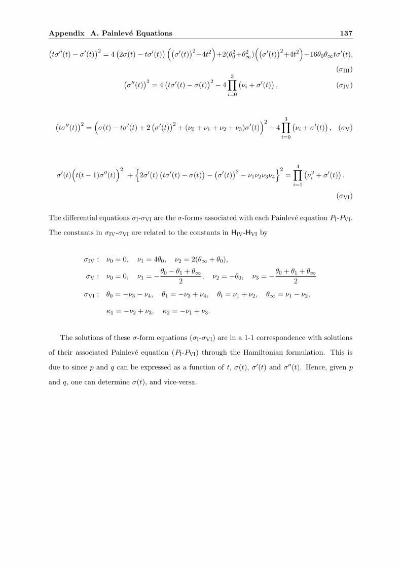
Appendix A. Painleve Equations 137

(tσ′′(t) − σ′(t)

)2 = 4(2σ(t) − tσ′(t)

) ((σ′(t)

)2−4t2)+2(θ2

0+θ2∞)((σ′(t)

)2+4t2)−16θ0θ∞tσ

′(t),

(σIII)(σ′′(t)

)2 = 4(tσ′(t) − σ(t)

)2 − 43∏

i=0

(νi + σ′(t)

), (σIV)

(tσ′′(t)

)2 =(σ(t) − tσ′(t) + 2

(σ′(t)

)2 + (ν0 + ν1 + ν2 + ν3)σ′(t))2

− 43∏

i=0

(νi + σ′(t)

), (σV)

σ′(t)(t(t− 1)σ′′(t)

)2+{

2σ′(t)(tσ′(t) − σ(t)

)−(σ′(t)

)2 − ν1ν2ν3ν4

}2=

4∏

i=1

(ν2i + σ′(t)

).

(σVI)

The differential equations σI-σVI are the σ-forms associated with each Painleve equation PI-PVI.

The constants in σIV-σVI are related to the constants in HIV-HVI by

σIV : ν0 = 0, ν1 = 4θ0, ν2 = 2(θ∞ + θ0),

σV : ν0 = 0, ν1 = −θ0 − θ1 + θ∞

2, ν2 = −θ0, ν3 = −

θ0 + θ1 + θ∞2

σVI : θ0 = −ν3 − ν4, θ1 = −ν3 + ν4, θt = ν1 + ν2, θ∞ = ν1 − ν2,

κ1 = −ν2 + ν3, κ2 = −ν1 + ν3.

The solutions of these σ-form equations (σI-σVI) are in a 1-1 correspondence with solutions

of their associated Painleve equation (PI-PVI) through the Hamiltonian formulation. This is

due to since p and q can be expressed as a function of t, σ(t), σ′(t) and σ′′(t). Hence, given p

and q, one can determine σ(t), and vice-versa.

138

Appendix B

Coefficients of Second Order

Difference Equation for βn

The recurrence coefficient βn satisfies a second order difference equation given by (4.21), which

turns out to be an algebraic equation of degree six in βn+1, βn and βn−1:

6∑

p=0

6∑

q=0

6∑

r=0

cp,q,rβpn+1β

qnβ

rn−1 = 0.

The coefficients cp,q,r depend upon n, k2, α and β. The 34 non-zero coefficients cp,q,r are given

as follows:

c0,0,0 = (k2 − 1)2n (n+ 2α) (n+ 2β) (n+ 2α+ 2β) . (B.1)

c0,1,0 = α2(−3 − 4β2 + 4α2)(k2 + 1)(k2 − 1)2(4(n+ α+ β)2 − 9

)(n+ α+ β)2

−29(4α2 − 1)(α2 − β2)(k2 + 1)(k2 − 1)2

(4(n+ α+ β)2 − 9

)(4(n+ α+ β)2 − 1

)

−19(4α4 − 4α2β2 − 19α2 − 8β2 + 18)(k2 + 1)(k2 − 1)2

(4(n+ α+ β)2 − 1

)(n+ α+ β)2

+2(k2 + 1)(n+ α+ β)2 − (α2 − β2)(16nα+ 16αβ + 1 + 16nβ + 8n2)(k2 − 1)2

+(4αβ + 2n2 − β2 + 5α2 + 4nα+ 4nβ)(k2 − 1)(k2 + 1). (B.2)

c0,1,1 = 8k2

(α+ β + n−

3

2

)[(k2 − 1)2(α+ β + n)3 +

1

2(k4 + 1)(α+ β + n)2

−(α2 + β2)(k2 − 1)2(α+ β + n) +1

2(k4 − 1)(α2 − β2)

], (B.3)

c1,1,0 = 8k2

(α+ β + n+

3

2

)[(k2 − 1)2(α+ β + n)3 −

1

2(k4 + 1)(α+ β + n)2

−(k2 − 1)2(α2 + β2)(α+ β + n) −1

2(k4 − 1)(α2 − β2)

], (B.4)

Appendix B. Coefficients of Second Order Difference Equation for βn 139

c0,2,0 = −8(k4 + 1)(k2 − 1)2(n+ α+ β)4 + 24(k2 + 1)2(k2 − 1)2(n+ α+ β)4 − 7(k4 + 1)(k2 + 1)2(n+ α+ β)2

+(k4 + 1)(k2 − 1)2(n+ α+ β)2(8α2 + 8β2 + 3) + 16(k2 + 1)(n+ α+ β)2(k2 − 1)2(k4 + 1)(α2 − β2)

−4(k2 + 1)2(k2 − 1)2(4k2(α2 − β2) + 6(α2 + β2) + 1

)(n+ α+ β)2 +

9

8(k4 + 1)(k2 + 1)2

−6(k2 − 1)(k2 + 1)2(k4 + 1)(α2 − β2) +1

8(k4 + 1)(k2 − 1)2(8α2 + 8β2 − 1)2

−2(k2 + 1)(k2 − 1)2(k4 + 1)(α2 − β2)(4α2 + 4β2 + 1)

+1

4(k4 − 1)2

(32k2(α2 − β2) − 8(α2 + β2) − 64α2β2 + 32k2(α4 − β4) − 1

), (B.5)

c1,1,1 = −8k4

(α+ β + n+

3

2

)(α+ β + n−

3

2

)[(k2 + 1)(α+ β + n)2 + (k2 − 1)(α2 − β2)

], (B.6)

c0,3,0 = −64k2

[1

8(k2 + 1)(8k4 − 15k2 + 8)(n+ α+ β)4 +

9

32(k2 + 1)(k4 + 1)

+3

64(k2 + 1)(k2 − 1)2

(11k2(α2 − β2) − 8(α2 + β2) − 2

)−

3

64(k4 + 1)(k2 − 1)(11k2 + 8)(α2 − β)2

−65

64(k4 + 1)(k2 + 1)(n+ α+ β)2 −

1

64(k2 + 1)(k2 − 1)2(n+ α+ β)2

(36k2(α2 − β2) + 32(α2 + β2) − 1

)

+17

32(n+ α+ β)2(k2 − 1)2(k4 + 1)(α2 − β2) +

1

32(k8 − 1)(n+ α+ β)2(α2 − β2)

], (B.7)

c1,2,0 = −32k2

(α+ β + n+

3

2

)[− (k2 + 1)(k2 − 1)2

(α2 +

1

4

)(α+ β + n) −

1

8(k4 − 1)(α+ β + n)(α2 − β2 + 2)

+7

8(k2 − 1)2(α+ β + n)(α2 − β2) −

1

4(k2 + 1)

(α+ β + n−

3

2

)−

1

8(k2 + 1)(k2 − 1)2(4α2 − 1)

−1

16(k4 − 1)(13α2 − 13β2 − 6) −

5

16(k2 − 1)2(α2 − β2) −

1

8(k2 + 1)(4k4 + 5k2 + 4)(α+ β + n)2

+1

4(k2 + 1)(4k4 − 9k2 + 4)(α+ β + n)3

], (B.8)

c0,2,1 = −32k2

(α+ β + n−

3

2

)[1

4(k2 + 1)(4k4 − 9k2 + 4)(α+ β + n)3 +

1

8(k2 + 1)(4k4 + 5k2 + 4)(α+ β + n)2

+1

8(k4 − 1)

(k2(4α2 − 1) + 5α2 − 9β2 − 2

)−

7

4(k2 − 1)(α2 − β2)

(α+ β + n+

5

14

)

−1

4(k4 − 1)

(k2(4α2 + 1) − 7α2 + 3β2

)(α+ β + n) −

1

4(k2 + 1)

(α+ β + n+

3

2

)]. (B.9)

c1,2,1 = 32k4

(α+ β + n+

3

2

)(α+ β + n−

3

2

)[(α+ β + n+

1

2

)(α+ β + n−

1

2

)(2k4 + k2 + 2

)−k2

2

],

(B.10)

c0,2,2 = 16k4

(α+ β + n−

3

2

)2[(

β + n+1

2

)(2α+ β + n+

1

2

)k4

+

(−3(α+ β + n)2 + α2 + β2 +

1

2

)k2 +

(α+ n+

1

2

)(α+ 2β + n+

1

2

)]

, (B.11)

c2,2,0 = 16k4

(α+ β + n+

3

2

)2[(

β + n−1

2

)(2α+ β + n−

1

2

)k4

+

(−3(α+ β + n)2 + α2 + β2 +

1

2

)k2 +

(α+ n−

1

2

)(α+ 2β + n−

1

2

)]

, (B.12)

c0,4,0 = k4

[32(3k4 − 2k2 + 3)(n+ α+ β)4 − 8

((4α2 + 22)k4 + (21 − 4α2 − 4β2)k2 + 4β2 + 22

)(n+ α+ β)2

+9

2(k4 + 1)(k2 − 1)(8α2 + 8β2 − 1) +

99

2(k2 + 1)(k4 + 1) − 9(k4 − 1)

(4k2(α2 + β2 +

5

4

)+ 4(α2 − β2)

)],

(B.13)

c1,3,0 = 32k4

(α+ β + n+

3

2

)[(k4 − 6k2 + 1)(α+ β + n)3 −

9

8(k4 + 1)

(α+ β + n−

13

6

)

+1

8(k2 − 1)(α+ β + n)(8k2α2 − 8β2 − k2 + 1) −

1

16(k2 − 1)

(40k2α2 − 40β2 + 17(k2 − 1)

)

−1

2(7k4 + 12k2 + 7)(α+ β + n)2

], (B.14)

Appendix B. Coefficients of Second Order Difference Equation for βn 140

c0,3,1 = 32k4

(α+ β + n−

3

2

)[−

9

8(k2 + 1)

(n+ α+ β +

13

6

)−

1

2(k4 − 1)(n+ α+ β)

(β2 − α2 +

9

8

)

+1

16(k2 − 1)2(n+ α+ β)(8α2 + 8β2 − 11) + (k4 − 6k2 + 1)(n+ α+ β)3

+1

16(k2 − 1)(40k2α2 − 22k2 − 40β2 − 17) +

1

2(7k4 + 12k2 + 7)(n+ α+ β)2

]. (B.15)

c1,3,1 = −128k6 (k2 + 1)(

α+ β + n+3

2

)(

α+ β + n−3

2

)(

(α+ β + n)2 −3

4

)

, (B.16)

c1,2,2 = −2k6(k2 + 1) (2α+ 2β + 2n− 3)2 (2α+ 2β + 2n+ 1) (2α+ 2β + 2n+ 3) , (B.17)

c2,2,1 = −2k6(k2 + 1) (2α+ 2β + 2n− 3) (2α+ 2β + 2n+ 3)2 (2α+ 2β + 2n− 1) , (B.18)

c0,4,1 = 32k6(k2 + 1)

(

α+ β + n−3

2

)[

(α+ β + n)2(

α+ β + n−19

2

)

+11

4(α+ β + n) +

39

8

]

,(B.19)

c1,4,0 = 32k6(k2 + 1)

(

α+ β + n+3

2

)[

(α+ β + n)2(

α+ β + n+19

2

)

+11

4(α+ β + n) −

39

8

]

,(B.20)

c0,3,2 = 2k6(k2 + 1) (2α+ 2β + 2n− 3)2 (2α+ 2β + 2n+ 1) (6α+ 6β + 6n− 7) , (B.21)

c2,3,0 = 2 k6(k2 + 1) (2α+ 2β + 2n+ 3)2 (6α+ 6β + 6n+ 7) (2α+ 2β + 2n− 1) , (B.22)

c0,5,0 = −64k6(k2 + 1)

(

α+ β + n+3

2

)(

α+ β + n−3

2

)[(

α+ β + n+1

2

)(

α+ β + n−1

2

)

−1

2

]

.

(B.23)

c2,4,0 = −112k8

(

α+ β + n+32

)2 [

(α+ β + n)2 +117

(α+ β + n) −3328

]

, (B.24)

c0,4,2 = −112k8

(

α+ β + n−32

)2 [

(n+ α+ β)

(

n+ α+ β −117

)

−3328

]

, (B.25)

c3,3,0 = −4k8 (2α+ 2n− 1 + 2β) (2α+ 2β + 2n+ 3)3 , (B.26)

c0,3,3 = −4 k8 (2α+ 2β + 2n− 3)3 (2α+ 2β + 2n+ 1) , (B.27)

c1,4,1 = 320k8

(

α+ β + n+32

)(

α+ β + n−32

)(

(α+ β + n)2 −1320

)

, (B.28)

c1,3,2 = 2 k8 (2α+ 2β + 2n− 3)2 (2α+ 2β + 2n+ 3)2 , (B.29)

c2,3,1 = 2 k8 (2α+ 2β + 2n− 3)2 (2α+ 2β + 2n+ 3)2 , (B.30)

c2,2,2 = k8 (2α+ 2β + 2n− 3)2 (2α+ 2β + 2n+ 3)2 , (B.31)

c1,5,0 = −32k8

(

α+ β + n+32

)2 [

(n+ α+ β) (n+ α+ β + 5) −154

]

, (B.32)

c0,5,1 = −32k8

(

α+ β + n−32

)2 [

(n+ α+ β) (n+ α+ β − 5) −154

]

, (B.33)

c0,6,0 = k8 (2α+ 2β + 2n− 3)2 (2α+ 2β + 2n+ 3)2 . (B.34)

141

Appendix C

Toeplitz+Hankel Determinants

The author would like to thank Prof. E. L. Basor for her input into this section.

In this appendix, we discuss how we can find the leading term of the large n expansion of

Dn[w(∙, k2)] = det

1∫

−1

xj+k (1 − x2)α(1 − k2x2)β dx

n−1

j,k=0

, α > −1, β ∈ R, k2 ∈ (0, 1), (C.1)

by reducing the Hankel determinant to another expansion of a certain Toeplitz+Hankel deter-

minant. For this certain Toeplitz+Hankel determinant, the leading order large n asymptotics

are known, calculated using the Riemann-Hilbert approach in [38].

From [8], the n× n Toeplitz and Hankel matrices with symbol1 a are defined by

Tn(a) =(aj−k

)n−1

j,k=0, Hn(a) =

(aj+k+1

)n−1

j,k=0, (C.2)

where ak are the Fourier coefficients

ak =12π

π∫

−π

a(eiθ)e−ikθ dθ, k ∈ Z, (C.3)

of an L1-function a(eiθ)

defined on the unit circle. The matrices Hn(a) are referred to as

Hankel matrices, however they are not the same as the Hankel matrices we consider in this

thesis, e.g. (C.1).

1Symbol is a synonym for generating function.

Appendix C. Toeplitz+Hankel Determinants 142

To make the connection, let us define, for b(x) an even function on [−1, 1], the following

determinant

detHn[b] = det

1π

1∫

−1

b(x)(2x)j+k dx

n−1

j,k=0

. (C.4)

An easy computation shows that

detHn[b] =2n(n−1)

πndet

1∫

−1

xj+k b(x) dx

n−1

j,k=0

. (C.5)

Therefore we would like to compute this determinant with b(x) = w(x, k2). From the computa-

tions in [8], we have that

detHn[b] = 2−2nα det(Tn(a) +Hn(a)), (C.6)

where

a(eiθ) = (1 − k2 cos2 θ)β (2 − 2 cos θ)α+1/2 (2 + 2 cos θ)α−1/2, θ ∈ (0, π]. (C.7)

The above is a finite determinant of Toeplitz+Hankel matrices. So the large n behavior of

Dn[w(∙, k2)] can be obtained from the large n behavior of detHn[w(∙, k2)], up to the factor

2−n(n−1)πn. Since a is even in θ, we can compute the determinant of the Toeplitz+Hankel

matrices using the result presented in [38]. We obtain

det(Tn(a) +Hn(a)) ∼ E np enG, (C.8)

where G, p and E are expressed in terms of the parameters of our weight, α, β and k2. We

have,

E :=(2π)απ1/2G2(1/2)

22(α2+αβ+β2)G2(α+ 1)∙

(1 +

√1 − k2

)2β(α+β)

(1 − k2)β(α+β/2), (C.9)

p := α2 − 1/4, (C.10)

enG :=

(1 +

√1 − k2

2

)2β n

. (C.11)

Appendix C. Toeplitz+Hankel Determinants 143

This means that, as n→ ∞, the leading order term in the expansion of Dn[w(∙, k2)] is given by

Dn[w(∙, k2)] ∼ E nα2−1/4 2−n(n+2α) (2π)n

(1 +

√1 − k2

2

)2β n

. (C.12)

The above result precisely agrees with the results from the ladder operator approach (4.185)

and the Coulomb fluid approach (4.180).

144

Appendix D

Amplify-and-Forward Wireless

Relay Model

Here we briefly recall the background for the Amplify-and-Forward relay model and give an

outline of the derivation of the moment generating function of the instantaneous SNR, (5.7):

Mγ(s) =

1n!

∫

[0,∞)n

∏

1≤j<k≤n(xj − xk)2

n∏

`=1

xm−n` e−x`

(1+a2x`

1+a2(1+ γsRNs

)x`

)Ns

dx`

1n!

∫

[0,∞)n

∏

1≤j<k≤n(xj − xk)2

n∏

`=1

xm−n` e−x` dx`

.

The above result was obtained in [44], where much of the material of this appendix can be

found.

D.1 Preliminaries

The MIMO communication system features a source, relay and destination terminal, having Ns,

NR and ND antennae respectively. In the process of transmitting a signal, each transmission

period is divided into two time slots. In the first time slot, the source transmits to the relay.

The relay then amplifies its received signal subject to an average power constraint, prior to

transmitting the amplified signal to the destination terminal during the second time-slot. We

assume that the source and destination terminals are sufficiently separated such that the direct

link between them is negligible (i.e., all communication is done via the relay).

Let H1 ∈ CNR×Ns and H2 ∈ CND×NR represent the channel matrices between the source

and relay, and the relay and destination terminals respectively. Each channel matrix is assumed

Appendix D. Amplify-and-Forward Wireless Relay Model 145

to have uncorrelated elements distributed as1 CN (0, 1). The destination is assumed to have

perfect knowledge of H2 and either H1 or the cascaded channel H2H1, while the relay and

source terminals have no knowledge of these.

A situation is considered where the source terminal transmits data using a method called

Orthogonal Space-Time Block Code (OSTBC) encoding [62]. In this situation, groups of indepen-

dent and identically distributed complex Gaussian random variables (referred to as information

“symbols”) si, i = 1, . . . , N are assigned via a special codeword mapping to a row orthogonal

matrix X = (x1, . . . ,xNP) ∈ CNs×NP satisfying the power constraint E

[‖xk‖2

]= γ, where γ

is the average received SNR at the relay, E is the expectation value, and NP is the number of

symbol periods used to send each codeword.

Since it takes NP symbol periods to transmit N symbols, the coding rate is then defined as

R =N

NP. (D.1)

The coding rate is dependent upon the particular OSTBC encoding method used, and typically

take the values2 1/2 (for rate 1/2 orthogonal design encoding), 2/3, 3/4, 5/6, 7/8 and 1 (for

full-rate Alamuti OSTBC encoding).

The received signal matrix at the relay terminal at the end of the first time slot,

Y = (y1, . . . ,yNP) ∈ CNR×NP ,

is given by

Y = H1X + N , (D.2)

where N ∈ CNR×NP has uncorrelated entries distributed as CN (0, 1), representing normalized

noise samples at the relay terminal. The relay then amplifies the signal it has received by a

constant gain matrix G = aINR, where

a2 =b

(1 + γ)NR. (D.3)

1The notation CN (μ, σ2) represents a complex Gaussian distribution with mean μ and variance σ2.

2With each encoding method, there are trade-offs between performance, efficiency and reliability.

D.2 Instantaneous Signal-to-Noise Ratio γ 146

In the above, b is the total power constraint imposed at the relay, i.e., E[‖Gyk‖

2]≤ b, whilst

γ represents the average received SNR at the relay. The received signal R ∈ CND×NP at the

destination terminal at the end of the second time slot is then given by

R = aH2Y + W = aH2H1X + aH2N + W, (D.4)

where W ∈ CND×NP has uncorrelated entries distributed as CN (0, 1), representing normalized

noise samples at the destination terminal.

Next, the receiver applies the linear (noise whitening) operation,

R = K−1/2R, K := a2H2H†2 + IND

, (D.5)

to yield the equivalent input-output model

R = HX + N, (D.6)

where H = aK−1/2H2H1 and N ∈ CND×NP has uncorrelated entries distributed as CN (0, 1).

D.2 Instantaneous Signal-to-Noise Ratio γ

Based on the above relationship, standard linear OSTBC decoding can be applied (see, e.g.,

[62]). This results in decomposing the matrix model (D.6) into a set of parallel non-interacting

single-input single-output relationships given by

si = ||H||F si + ηi, l = 1, . . . , N,

where ηi is distributed as CN (0, 1), with ||H||F representing the Frobenius norm (or matrix

norm) of H.

The quantity that we are interested in, the instantaneous SNR for the ith symbol γi, can

then be written as

γi = ||H||2FE[|si|

2]

=γa2

RNsTr(H†

1H†2K

−1H2H1

). (D.7)

Since the right-hand side is independent of i, we may drop the i subscript and denote the

instantaneous SNR as γ without loss of generality.

Appendix D. Amplify-and-Forward Wireless Relay Model 147

D.3 Derivation of Moment Generating Function Mγ(s)

By definition, the moment generating function of the instantaneous SNR γ is then given by

Mγ(s) = Eγ [exp(−sγ)] , (D.8)

= EH1,H2

[

−γa2s

RNsTr(H†

1H†2K

−1H2H1

)]

, (D.9)

= EH2

1

det(IND

+ a2γsRNs

H†2K

−1H2

)

, (D.10)

where the third equality is from a result in [96]. Using SVD (singular value decomposition)

factorization [99] on H2 then yields

Mγ|X (s) =n∏

i=1

1 + a2xi

1 + a2(1 + γs

RNs

)xi

Ns

, (D.11)

where n = min(NR, ND), X = diag(x1, x2, . . . , xn) and xi, i = 1, 2, . . . , n, are the eigenvalues3

of H2†H2.

Since H2†H2 is a Wishart random matrix, its joint distribution of eigenvalues is given by

[110] as equation (1.2) with the weight function w0(x) = x|NR−ND|e−x, x ∈ [0,∞) (This is the

Laguerre weight with α = |NR − ND|). The moment generating function (5.7) then follows

from averaging (D.11) with respect to the joint distribution of eigenvalues of Wishart random

matrices.

3The singular values of H2, σi, i = 1, 2, . . . , n, are related to related to the eigenvalues of H2†H2 by σ 2

i =xi > 0

148

Appendix E

Proof of Theorem 5.1

In this appendix, we provide the proof to Theorem 5.1, which gives the PDE satisfied by the

Hankel determinant generated via

wAF(x) = xαe−x(t+ x

T + x

)Ns

. (E.1)

E.1 Computation of Auxiliary Variables

With our weight function given by (E.1), we can construct the associated potential v(x) through

(2.28) as

v(x) = − logwAF(x) = x− α log x−Ns log

(t+ x

T + x

)

, (E.2)

and therefore,

v′(x) = 1 −α

x−

Ns

x+ t+

Ns

x+ T. (E.3)

Hence

v′(x) − v′(y)x− y

=α

xy+

Ns

(x+ t)(y + t)−

Ns

(x+ T )(y + T ). (E.4)

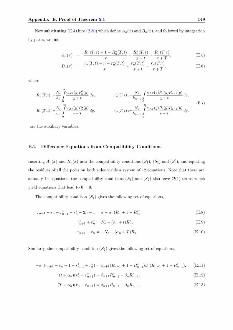
Appendix E. Proof of Theorem 5.1 149

Now substituting (E.4) into (2.30) which define An(x) and Bn(x), and followed by integration

by parts, we find

An(x) =Rn(T, t) + 1 −R∗

n(T, t)x

+R∗n(T, t)x+ t

−Rn(T, t)x+ T

, (E.5)

Bn(x) =rn(T, t) − n− r∗n(T, t)

x+r∗n(T, t)x+ t

−rn(T, t)x+ T

, (E.6)

where

R∗n(T, t) :=

Ns

hn

∞∫

0

wAF(y)P 2n(y)

y + tdy, r∗n(T, t) :=

Ns

hn−1

∞∫

0

wAF(y)Pn(y)Pn−1(y)y + t

dy,

Rn(T, t) :=Ns

hn

∞∫

0

wAF(y)P 2n(y)

y + Tdy, rn(T, t) :=

Ns

hn−1

∞∫

0

wAF(y)Pn(y)Pn−1(y)y + T

dy,

(E.7)

are the auxiliary variables.

E.2 Difference Equations from Compatibility Conditions

Inserting An(x) and Bn(x) into the compatibility conditions (S1), (S2) and (S′2), and equating

the residues of all the poles on both sides yields a system of 12 equations. Note that there are

actually 14 equations, the compatibility conditions (S1) and (S2) also have O(1) terms which

yield equations that lead to 0 = 0.

The compatibility condition (S1) gives the following set of equations,

rn+1 + rn − r∗n+1 − r∗n − 2n− 1 = α− αn(Rn + 1 −R∗n), (E.8)

r∗n+1 + r∗n = Ns − (αn + t)R∗n, (E.9)

−rn+1 − rn = −Ns + (αn + T )Rn. (E.10)

Similarly, the compatibility condition (S2) gives the following set of equations,

−αn(rn+1 − rn − 1 − r∗n+1 + r∗n) = βn+1(Rn+1 + 1 −R∗n+1)βn(Rn−1 + 1 −R∗

n−1), (E.11)

(t+ αn)(r∗n − r∗n+1) = βn+1R

∗n+1 − βnR

∗n−1, (E.12)

(T + αn)(rn − rn+1) = βn+1Rn+1 − βnRn−1. (E.13)

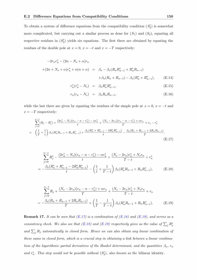
E.2 Difference Equations from Compatibility Conditions 150

To obtain a system of difference equations from the compatibility condition (S′2) is somewhat

more complicated, but carrying out a similar process as done for (S1) and (S2), equating all

respective residues in (S′2) yields six equations. The first three are obtained by equating the

residues of the double pole at x = 0, x = −t and x = −T respectively:

−2rnr∗n − (2n−Ns + α)rn

+(2n+Ns + α)r∗n + n(n+ α) = βn − βn(RnR∗n−1 +R∗

nRn−1)

+βn(Rn +Rn−1) − βn(R∗n +R∗

n−1), (E.14)

r∗n(r∗n −Ns) = βnR

∗nR

∗n−1, (E.15)

rn(rn −Ns) = βnRnRn−1, (E.16)

while the last three are given by equating the residues of the simple pole at x = 0, x = −t and

x = −T respectively:

n−1∑

j=0

(Rj −R∗j ) +

(2r∗n −Ns)(rn − n− r∗n) − αr∗nt

+(Ns − 2rn)(rn − n− r∗n) + αrn

T+ rn − r∗n

=

(1

T+

1

t

)

βn(R∗nRn−1 +RnR

∗n−1) +

βn(R∗n +R∗

n−1 − 2R∗nR

∗n−1)

t−βn(Rn +Rn−1 + 2RnRn−1)

T,

(E.17)

n−1∑

j=0

R∗j −

(2r∗n −Ns)(rn − n− r∗n) − αr∗nt

+(Ns − 2rn)r∗n +Nsrn

T − t+ r∗n

= −βn(R∗

n +R∗n−1 − 2R∗

nR∗n−1)

t−

(1t

+1

T − t

)

βn(R∗nRn−1 +RnR

∗n−1), (E.18)

n−1∑

j=0

Rj +(Ns − 2rn)(rn − n− r∗n) + αrn

T+

(Ns − 2rn)r∗n +NsrnT − t

+ rn

= −βn(Rn +Rn−1 + 2RnRn−1)

T+

(1T

−1

T − t

)

βn(R∗nRn−1 +RnR

∗n−1). (E.19)

Remark 17. It can be seen that (E.17) is a combination of (E.18) and (E.19), and serves as a

consistency check. We also see that (E.18) and (E.19) respectively gives us the value of∑

j R∗j

and∑

j Rj automatically in closed form. Hence we can also obtain any linear combination of

these sums in closed form, which is a crucial step in obtaining a link between a linear combina-

tion of the logarithmic partial derivatives of the Hankel determinant, and the quantities βn, rn

and r∗n. This step would not be possible without (S′2), also known as the bilinear identity.

Appendix E. Proof of Theorem 5.1 151

E.3 Analysis of Non-linear System

Whilst some of the above difference equations (E.8)–(E.19) look rather complicated, our aim is

to manipulate these equations in such a way as to give us insight into the recurrence coefficients

αn and βn. Our dominant strategy is to always try to describe the recurrence coefficients αn

and βn in terms of the auxiliary variables Rn, rn, R∗n and r∗n.

The first thing we can do is to sum (E.8) through (E.10) to get a simple expression for the

recurrence coefficient αn in terms of the auxiliary variables Rn and R∗n:

αn = TRn − tR∗n + α+ 2n+ 1. (E.20)

We can immediately see that by taking a telescopic sum of the above from j = 0 to j = n− 1,

and recalling equation (2.18), gives rise to

Tn−1∑

j=0

Rj − tn−1∑

j=0

R∗j + n(n+ α) =

n−1∑

j=0

αj ,

= −p1(n). (E.21)

Looking at (S2) next, we sum equations (E.11) through (E.13) to get

αn = βn+1 − βn + T (rn − rn+1) + t(r∗n+1 − r∗n). (E.22)

Taking a telescopic sum of the above from j = 0 to j = n− 1 and rearranging yields

βn = Trn − tr∗n − p1(n). (E.23)

We are now in a position to derive the following important lemma, which describes the recurrence

coefficients αn and βn in terms of the set of auxiliary variables.

Lemma E.1. The quantities αn and βn are given in terms of the auxiliary variables Rn, rn,

R∗n and r∗n as

αn = TRn − tR∗n + α+ 2n+ 1, (E.24)

βn =1

1 +Rn −R∗n

[

(1 +Rn)r∗n(r

∗n −Ns)R∗n

+ (R∗n − 1)

rn(rn −Ns)Rn

− 2rnr∗n

−(2n−Ns + α)rn + (2n+Ns + α)r∗n + n(n+ α)

]

. (E.25)

E.4 Toda Evolution 152

Proof. Equation (E.24) is a restatement of equation (E.20).

To obtain (E.25), we use the equations obtained from(S′2). We eliminate R∗

n−1 and Rn−1

from (E.14) using (E.15) and (E.16) respectively, and then rearrange to express βn in terms of

the auxiliary quantities.

E.4 Toda Evolution

In this section, n is kept fixed while we vary two parameters in the weight function (5.15),

namely T and t. The other parameters, α and Ns are kept fixed.

Differentiating the orthogonality condition (2.12), w.r.t. T and t, for m = n, gives

∂T (log hn) = −Rn, (E.26)

∂t(log hn) = R∗n (E.27)

respectively. Then, from equation (2.19), i.e. βn = hn/hn−1, it follows that

∂Tβn = βn(Rn−1 −Rn), (E.28)

∂tβn = βn(R∗n −R∗

n−1). (E.29)

Applying ∂T and ∂t to the orthogonality relation

∞∫

0

Pn(x)Pn−1(x)wAF(x, T, t) dx = 0,

results in the following two relations:

∂Tp1(n) = rn, (E.30)

∂tp1(n) = −r∗n. (E.31)

Note that in the above computations with ∂t and ∂T we must keep in mind that the coeffi-

cients of Pn(x) depend on t and T.

Appendix E. Proof of Theorem 5.1 153

Using the above two equations, we get that

(T∂T + t∂t)p1(n) = Trn − tr∗n,

= p1(n) + βn, (E.32)

where the second equality follows from (E.23).

Using equation (2.17), i.e. αn = p1(n) − p1(n+ 1), we get that

∂Tαn = rn − rn+1, (E.33)

∂tαn = r∗n+1 − r∗n. (E.34)

Now, combining (E.33), (E.34), (E.23), and (2.17), and similarly using (E.24), (E.28) and

(E.29), we arrive at the following lemma:

Lemma E.2. The recurrence coefficients αn and βn satisfy the following partial differential

relations:

(T∂T + t∂t − 1)αn = βn − βn+1, (E.35)

(T∂T + t∂t − 2)βn = βn(αn−1 − αn). (E.36)

In the second of the above two equations, we eliminate αn using the first equation to derive a

second order differential-difference relation for βn:

(T 2∂2TT + 2Tt∂2

Tt + t2∂2tt) log βn = βn−1 − 2βn + βn+1 − 2, (E.37)

which is a two-variable generalization of the Toda equations [97].

Now, before proceeding to examine the time-evolution behaviour of the Hankel determinant,

we state the following lemmas regarding the auxiliary variables Rn, R∗n, rn and r∗n.

Lemma E.3. The auxiliary variables Rn, R∗n, rn and r∗n satisfy the following first order PDE

system:

T∂TRn − t∂TR∗n =

[TRn − tR∗

n + 2n+ α+ T]Rn + 2rn −Ns, (E.38)

T∂tRn − t∂tR∗n =

[− TRn + tR∗

n − 2n− α− t]R∗n − 2r∗n +Ns, (E.39)

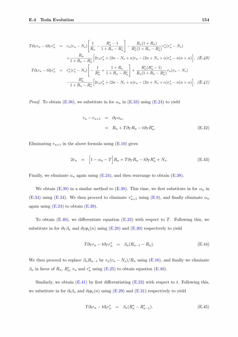
E.4 Toda Evolution 154

T∂T rn − t∂T r∗n = rn(rn −Ns)

[1Rn

−R∗

n − 11 +Rn −R∗

n

]

−Rn(1 +Rn)

R∗n(1 +Rn −R∗

n)r∗n(r∗n −Ns)

+Rn

1 +Rn −R∗n

[2rnr

∗n + (2n−Ns + α)rn − (2n+Ns + α)r∗n − n(n+ α)

], (E.40)

T∂trn − t∂tr∗n = r∗n(r∗n −Ns)

[

−1R∗

n

+1 +Rn

1 +Rn −R∗n

]

+R∗

n(R∗n − 1)

Rn(1 +Rn −R∗n)rn(rn −Ns)

−R∗

n

1 +Rn −R∗n

[2rnr

∗n + (2n−Ns + α)rn − (2n+Ns + α)r∗n − n(n+ α)

]. (E.41)

Proof. To obtain (E.38), we substitute in for αn in (E.33) using (E.24) to yield

rn − rn+1 = ∂Tαn,

= Rn + T∂TRn − t∂TR∗n. (E.42)

Eliminating rn+1 in the above formula using (E.10) gives

2rn =[1 − αn − T

]Rn + T∂TRn − t∂TR

∗n +Ns. (E.43)

Finally, we eliminate αn again using (E.24), and then rearrange to obtain (E.38).

We obtain (E.39) in a similar method to (E.38). This time, we first substitute in for αn in

(E.34) using (E.24). We then proceed to eliminate r∗n+1 using (E.9), and finally eliminate αn

again using (E.24) to obtain (E.39).

To obtain (E.40), we differentiate equation (E.23) with respect to T . Following this, we

substitute in for ∂Tβn and ∂Tp1(n) using (E.28) and (E.30) respectively to yield

T∂T rn − t∂T r∗n = βn(Rn−1 −Rn). (E.44)

We then proceed to replace βnRn−1 by rn(rn −Ns)/Rn using (E.16), and finally we eliminate

βn in favor of Rn, R∗n, rn and r∗n using (E.25) to obtain equation (E.40).

Similarly, we obtain (E.41) by first differentiating (E.23) with respect to t. Following this,

we substitute in for ∂tβn and ∂tp1(n) using (E.29) and (E.31) respectively to yield

T∂trn − t∂tr∗n = βn(R

∗n −R∗

n−1). (E.45)

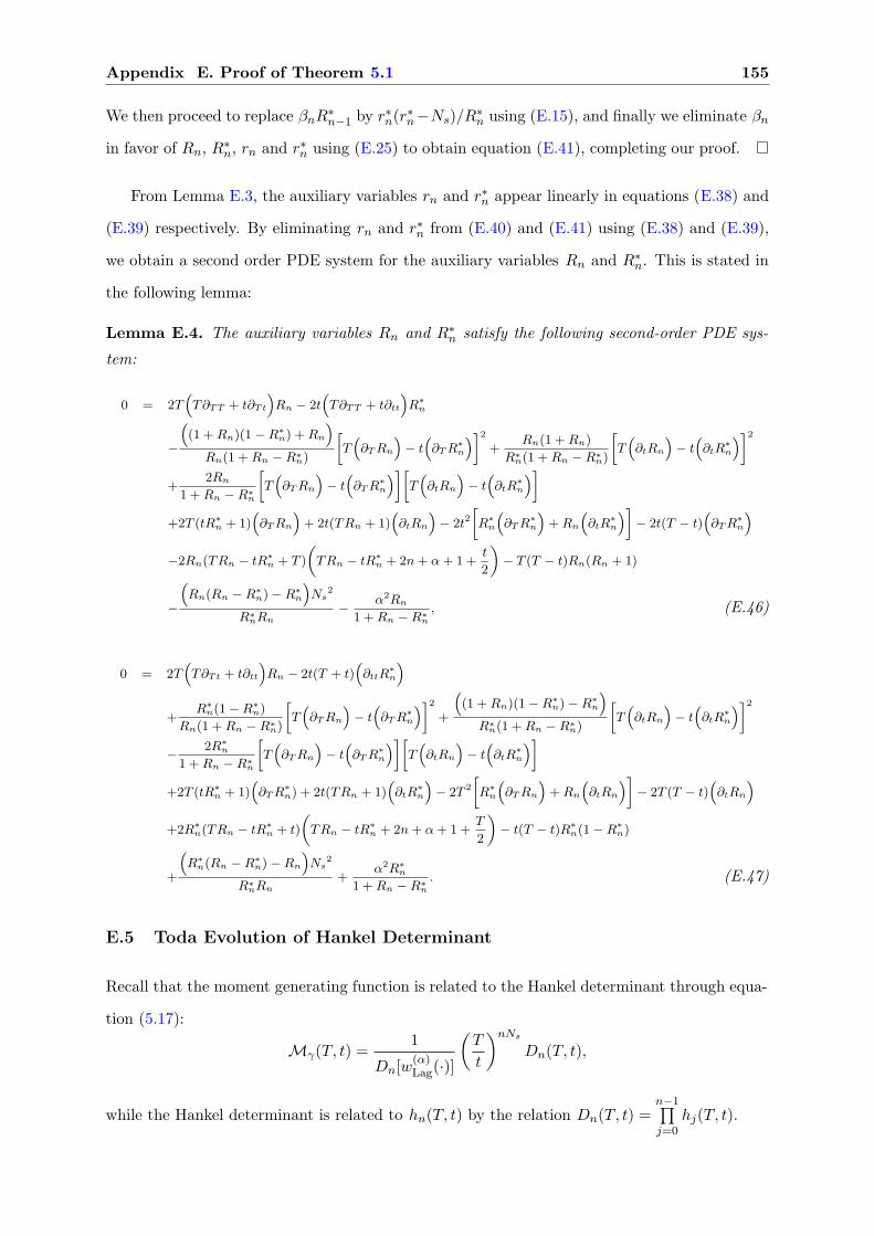
Appendix E. Proof of Theorem 5.1 155

We then proceed to replace βnR∗n−1 by r∗n(r

∗n−Ns)/R∗

n using (E.15), and finally we eliminate βn

in favor of Rn, R∗n, rn and r∗n using (E.25) to obtain equation (E.41), completing our proof.

From Lemma E.3, the auxiliary variables rn and r∗n appear linearly in equations (E.38) and

(E.39) respectively. By eliminating rn and r∗n from (E.40) and (E.41) using (E.38) and (E.39),

we obtain a second order PDE system for the auxiliary variables Rn and R∗n. This is stated in

the following lemma:

Lemma E.4. The auxiliary variables Rn and R∗n satisfy the following second-order PDE sys-

tem:

0 = 2T(T∂TT + t∂Tt

)Rn − 2t

(T∂TT + t∂tt

)R∗

n

−

((1 +Rn)(1 −R∗

n) +Rn

)

Rn(1 +Rn −R∗n)

[

T(∂TRn

)− t(∂TR

∗n

)]2+

Rn(1 +Rn)

R∗n(1 +Rn −R∗

n)

[

T(∂tRn

)− t(∂tR

∗n

)]2

+2Rn

1 +Rn −R∗n

[

T(∂TRn

)− t(∂TR

∗n

)][

T(∂tRn

)− t(∂tR

∗n

)]

+2T (tR∗n + 1)

(∂TRn

)+ 2t(TRn + 1)

(∂tRn

)− 2t2

[

R∗n

(∂TR

∗n

)+Rn

(∂tR

∗n

)]

− 2t(T − t)(∂TR

∗n

)

−2Rn(TRn − tR∗n + T )

(

TRn − tR∗n + 2n+ α+ 1 +

t

2

)

− T (T − t)Rn(Rn + 1)

−

(Rn(Rn −R∗

n) −R∗n

)Ns

2

R∗nRn

−α2Rn

1 +Rn −R∗n

, (E.46)

0 = 2T(T∂Tt + t∂tt

)Rn − 2t(T + t)

(∂ttR

∗n

)

+R∗

n(1 −R∗n)

Rn(1 +Rn −R∗n)

[

T(∂TRn

)− t(∂TR

∗n

)]2+

((1 +Rn)(1 −R∗

n) −R∗n

)

R∗n(1 +Rn −R∗

n)

[

T(∂tRn

)− t(∂tR

∗n

)]2

−2R∗

n

1 +Rn −R∗n

[

T(∂TRn

)− t(∂TR

∗n

)][

T(∂tRn

)− t(∂tR

∗n

)]

+2T (tR∗n + 1)

(∂TR

∗n) + 2t(TRn + 1)

(∂tR

∗n

)− 2T 2

[

R∗n

(∂TRn

)+Rn

(∂tRn

)]

− 2T (T − t)(∂tRn

)

+2R∗n(TRn − tR∗

n + t)

(

TRn − tR∗n + 2n+ α+ 1 +

T

2

)

− t(T − t)R∗n(1 −R∗

n)

+

(R∗

n(Rn −R∗n) −Rn

)Ns

2

R∗nRn

+α2R∗

n

1 +Rn −R∗n

. (E.47)

E.5 Toda Evolution of Hankel Determinant

Recall that the moment generating function is related to the Hankel determinant through equa-

tion (5.17):

Mγ(T, t) =1

Dn[w(α)Lag(∙)]

(T

t

)nNs

Dn(T, t),

while the Hankel determinant is related to hn(T, t) by the relation Dn(T, t) =n−1∏

j=0hj(T, t).

E.5 Toda Evolution of Hankel Determinant 156

We compute the partial derivatives of the Hankel determinant by taking a telescopic sum

from j = 0 to j = n − 1 of the partial derivatives of log hn, i.e. equations (E.26) and (E.27).

Using (2.13), we then obtain

∂T (logDn) = −n−1∑

j=0

Rj , (E.48)

∂t(logDn) =n−1∑

j=0

R∗j . (E.49)

Hence we now have expressions of the partial derivatives of Dn(T, t) in terms of the auxiliary

variables Rn and R∗n.

At this point, recalling equation (5.36) that

Hn(T, t) = (T∂T + t∂t) logDn(T, t). (E.50)

This quantity related to the logarithmic derivative of the Hankel determinant is of special

interest as our goal is to find the PDE that Hn(T, t) satisfies. From the definition of Hn(T, t),

along with (E.48) and (E.49), we find that

Hn(T, t) = −Tn−1∑

j=0

Rj + tn−1∑

j=0

R∗j , (E.51)

= p1(n) + n(n+ α), (E.52)

where the second equality is a result of (E.21).

At this point, we may express the fundamental quantity Hn(T, t) in terms of the auxiliary

variables and βn. This is given in the following key lemma.

Lemma E.5.

Hn(T, t) = 2rnr∗n + (2n−Ns + α+ T )rn − (2n+Ns + α+ t)r∗n

−(1 +Rn)r∗n(r

∗n −Ns)R∗n

+ (1 −R∗n)rn(rn −Ns)

Rn+ βnRn − βnR

∗n. (E.53)

Proof. Using (E.18) and (E.19), we obtain the sum

t

n−1∑

j=0

R∗j − T

n−1∑

j=0

Rj

Appendix E. Proof of Theorem 5.1 157

in closed form. All that remains is to eliminate R∗n−1 and Rn−1 from this equation. We do this

using (E.15) and (E.16).

To continue, we apply t∂T + t∂t to equation (E.52), and find that

(T∂T + t∂t)Hn = p1(n) + βn, (E.54)

where we have used (E.32) to replace (T∂T + t∂t)p1(n) by p1(n) + βn.

We see that equations (E.52) and (E.54) can be regarded as a set of simultaneous equations

for p1(n) and βn. Solving for p1(n) and βn, we find that

p1(n) = Hn − n(n+ α), (E.55)

and

βn = (T∂T + t∂t)Hn −Hn + n(n+ α). (E.56)

Before completing the proof of Theorem 5.1, we show here that our Hankel determinant

Dn(T, t) is related to the τ -function of a Toda PDE. This is stated in the following lemma:

Lemma E.6. Defining

Dn(T, t) := (Tt)−n(n+α)

2 Dn(T, t), (E.57)

then Dn(T, t) satisfies the following equation:

(T

t∂2TT + 2∂2

Tt +t

T∂2tt

)

log Dn(T, t) =Dn+1Dn−1

D2n

. (E.58)

Proof. Substituting the definition (5.36) into (E.56) and together with (2.21), we find

(T∂T + t∂t)2 logDn − (T∂T + t∂t) logDn + n(n+ α) =

Dn+1Dn−1

D2n

.

Defining Dn(T, t) by (E.57) and after some computations, we obtain equation (E.58).

The above equation is a two parameter generalization of the Toda molecule equation [97],

and hence we identify Dn(T, t) as the corresponding τ -function of the two-parameter Toda

equations.

E.6 Partial Differential Equation for Hn(T, t) 158

A reduction may be obtained by writing Dn(T, t) as

Dn(T, t) =

(T

t

)n(n+α)2

Φn(T ),

and equation (E.58) is reduced to a 1-parameter Toda equation,

∂2TT log Φn(T ) =

Φn+1(T )Φn−1(T )Φn(T )2

.

E.6 Partial Differential Equation for Hn(T, t)

We differentiate (E.52) with respect to T and t, and make use of the expressions for ∂Tp1(n)

and ∂tp1(n), i.e., (E.30) and (E.31) respectively, to give

∂THn = rn, (E.59)

∂tHn = −r∗n . (E.60)

Thus, we now have expressed rn and r∗n in terms of the partial derivatives of Hn.

Next we derive representations of Rn and R∗n in terms of Hn and its partial derivatives.

The idea, following from previous work [12], is to find two quadratic equations, one satisfied

by Rn, the other by R∗n, where the coefficients of these quadratic equations are dependent on

Hn and its partial derivatives, and T , t, n, α and Ns.

We start by re-writing (E.16) as

βn Rn−1 =rn(rn −Ns)

Rn,

and substitute into (E.28) to arrive at

∂Tβn =rn(rn −Ns)

Rn− βnRn. (E.61)

Substituting rn given by (E.59) and βn given by (E.56) into the above equation produces

(T∂2TT + t∂2

Tt)Hn =(∂THn)

(∂THn −Ns

)

Rn

−(T (∂THn) + t(∂tHn) −Hn + n(n+ α)

)Rn. (E.62)

Appendix E. Proof of Theorem 5.1 159

Going through a similar process we find, using (E.15), (E.56) and (E.60),

(T∂2Tt + t∂2

tt)Hn = −(∂tHn)

(∂tHn +Ns

)

R∗n

+(T (∂THn) + t(∂tHn) −Hn + n(n+ α)

)R∗n. (E.63)

The above two equations are quadratic equations in Rn and R∗n. Solving for them leads to

2(T (∂THn) + t(∂tHn) −Hn + n(n+ α)

)Rn = −(T∂2

TT + t∂2Tt)Hn ± Δ1(Hn), (E.64)

2(T (∂THn) + t(∂tHn) −Hn + n(n+ α)

)R∗n = (T∂2

Tt + t∂2tt)Hn ± Δ2(Hn), (E.65)

where Δi(Hn), i = 1, 2, are defined by (5.39) and (5.40) respectively, where we have left out

the notation that indicates that the functions Δ1 and Δ2 are also dependent on the partial

derivatives of Hn.

In the last step we substitute (E.59), (E.60), (E.56), Rn given by (E.64) and R∗n given by

(E.65) into (E.53). After some simplification, we obtain the PDE (5.38), completing the proof

of Theorem 5.1.

160

Appendix F

Proof of Theorem 5.2

In this appendix we provide a proof for Theorem 5.2, which gives the PDE satisfied by the

Hankel determinant generated via (5.53),

w(x, ξ, η) = xαe−xeξ

x+η . (F.1)

F.1 Computation of Auxiliary Variables

The associated potential v(x) can be constructed through (2.28) as (dropping subscripts and ξ,

η dependence notation)

v(x) = − logw(x) = x− α log x−ξ

x+ η, (F.2)

v′(x) = 1 −α

x+

ξ

(x+ η)2, (F.3)

and therefore

v′(x) − v′(y)x− y

=α

xy−

ξ

(x+ η)2(y + η)−

ξ

(x+ η)(y + η)2. (F.4)

Now substituting (F.3) and (F.4) into the definitions of An(x) and Bn(x), (2.30), and inte-

grating by parts, we find that

An(x) =1 +R∗

n(ξ, η)x

−R∗n(ξ, η)x+ η

−ξRn(ξ, η)(x+ η)2

, (F.5)

Bn(x) =r∗n(ξ, η) − n

x−r∗n(ξ, η)x+ η

−ξrn(ξ, η)(x+ η)2

, (F.6)

Appendix F. Proof of Theorem 5.2 161

where we introduce the auxiliary quantities

R∗n(ξ, η) :=

ξ

hn

∞∫

0

w(y)P 2n(y)

(y + η)2dy, r∗n(ξ, η) :=

ξ

hn−1

∞∫

0

w(y)Pn(y)Pn−1(y)(y + η)2

dy,

Rn(ξ, η) :=1hn

∞∫

0

w(y)P 2n(y)

y + ηdy, rn(ξ, η) :=

1hn−1

∞∫

0

w(y)Pn(y)Pn−1(y)y + η

dy.

(F.7)

F.2 Difference Equations from Compatibility Conditions

Inserting An(x) and Bn(x) into the compatibility conditions (S1), (S2) and (S′2): and equating

the residues of all the poles on both sides yields a system of twelve equations. Note that there

are actually 14 equations, the compatibility conditions (S1) and (S2) also have O(x0) terms

which yield equations that lead to 0 = 0.

The compatibility condition (S1) gives the following set of equations:

r∗n+1 + r∗n − 2n− 1 = α− αn(1 +R∗n), (F.8)

r∗n+1 + r∗n = ξRn − (αn + η)R∗n, (F.9)

rn+1 + rn = 1 − (αn + η)Rn. (F.10)

Similarly, the compatibility condition (S2) gives the following set of equations:

αn(r∗n − r∗n+1 + 1) = βn+1(1 +R∗

n+1) − βn(1 +R∗n−1), (F.11)

(η + αn)(r∗n − r∗n+1) + ξrn+1 − ξrn = βn+1R

∗n+1 − βnR

∗n−1, (F.12)

(η + αn)(rn − rn+1) = βn+1Rn+1 − βnRn−1. (F.13)

Finally, the first three equations from (S′2) are given by equating the residues of the double pole

at x = 0, triple pole at x = −η, and pole of order four at x = −η respectively:

(r∗n − n)(r∗n − n− α) = βn(1 +R∗n)(1 +R∗

n−1), (F.14)

r∗n(2rn − 1) = βn(R∗nRn−1 +RnR

∗n−1), (F.15)

rn(rn − 1) = βnRnRn−1, (F.16)

F.3 Analysis of Non-linear System 162

while the last three are given by equating the residues of the pole at x = 0 and x = −η; and

the double pole at x = −η respectively:

n−1∑

j=0

R∗j + r∗n +

(α− 2r∗n)(r∗n − n) + nα

η+

ξ

η2

(αrn − (2rn − 1)(r∗n − n)

)

= −βnη

(R∗n +R∗

n−1 + 2R∗nR

∗n−1) −

ξβnη2

(Rn +Rn−1 +RnR∗n−1 +R∗

nRn−1), (F.17)

−n−1∑

j=0

R∗j − r∗n +

(2r∗n − α)(r∗n − n) − nα

η+

ξ

η2

((2rn − 1)(r∗n − n) − αrn

)

=βnη

(R∗n +R∗

n−1 + 2R∗nR

∗n−1) +

ξβnη2

(Rn +Rn−1 +RnR∗n−1 +R∗

nRn−1), (F.18)

−ξn−1∑

j=0

Rj + r∗n2 − ξrn +

ξ

η

((2rn − 1)(r∗n − n) − αrn

)

=ξβnη

(Rn +Rn−1 +RnR∗n−1 +R∗

nRn−1) + βnR∗nR

∗n−1. (F.19)

Remark 18. It can be observed that (F.17) and (F.18) are equivalent, and serve as a consistency

check.

F.3 Analysis of Non-linear System

Whilst some of the above difference equations (F.8)–(F.19) look rather complicated, our aim is

to manipulate these equations in such a way1 as to give us insight into the recurrence coefficients

αn and βn.

The first thing we can do is to sum (F.8) and (F.9) to get a simple expression for the

recurrence coefficient αn in terms of the auxiliary variables Rn and R∗n:

αn = ηR∗n − ξRn + α+ 2n+ 1, (F.20)

1Recall: Our dominant strategy is to always try to describe the recurrence coefficients αn and βn in terms ofthe auxiliary variables Rn, rn, R∗

n and r∗n.

Appendix F. Proof of Theorem 5.2 163

We can immediately see that by taking a telescopic sum of the above from j = 0 to j = n− 1,

and remembering equation (2.18), we get that

ηn−1∑

j=0

R∗j − ξ

n−1∑

j=0

Rj + n(n+ α) =n−1∑

j=0

αj ,

= −p1(n). (F.21)

Looking at (S2) next, subtracting equations (F.12) from (F.11) leads to

αn = βn+1 − βn + η(r∗n − r∗n+1) + ξ(rn+1 − rn). (F.22)

Taking a telescopic sum of the above from j = 0 to j = n− 1 and rearranging yields

βn = ηr∗n − ξrn − p1(n). (F.23)

Lemma F.1. The quantities αn and βn are given in terms of the auxiliary variables Rn, rn,

R∗n and r∗n as

αn = ηR∗n − ξRn + α+ 2n+ 1, (F.24)

βn =1Rn

(Rn

1 +R∗n

(r∗n − n)(r∗n − n− α) +R∗n

Rnrn(rn − 1) − r∗n(2rn − 1)

)

. (F.25)

Proof. Equation (F.24) is a restatement of equation (F.20).

To obtain (F.25), we use the equations obtained from(S′2). We eliminate R∗

n−1 and Rn−1

from (F.15) using (F.14) and (F.16) respectively, and then rearrange to express βn in terms of

the auxiliary quantities.

F.4 Toda Evolution

In this section, n is kept fixed while we vary two parameters in the weight function (F.1), namely

ξ and η. The other parameter, α is also kept fixed since it only takes discrete values.

Differentiating the definition of hn, equation (2.12), w.r.t. ξ and η, for m = n, gives

∂ξ(log hn) = Rn, (F.26)

∂η(log hn) = −R∗n, (F.27)

F.4 Toda Evolution 164

Then, from equation (2.19), i.e. βn = hn/hn−1, it follows that

∂ξβn = βn(Rn −Rn−1), (F.28)

∂ηβn = βn(R∗n−1 −R∗

n). (F.29)

Applying ∂ξ and ∂η to the orthogonality relation

∞∫

0

Pn(x)Pn−1(x)w(x, ξ, η) dx = 0,

results in the following two relations:

∂ξp1(n) = −rn, (F.30)

∂ηp1(n) = r∗n. (F.31)

Using the above two equations, we get that

(ξ∂ξ + η∂η)p1(n) = ηr∗n − ξrn,

= p1(n) + βn, (F.32)

where the second equality follows from (F.23).

Using equation (2.17), i.e. αn = p1(n) − p1(n+ 1), we get that

∂ξαn = rn+1 − rn, (F.33)

∂ηαn = r∗n − r∗n+1. (F.34)

Now, combining (F.33), (F.34), (F.23), and (2.17), and similarly using (F.24), (F.28) and

(F.29), we arrive at the following lemma:

Lemma F.2. The recurrence coefficients αn and βn satisfy the following partial differential

relations:

(ξ∂ξ + η∂η − 1)αn = βn − βn+1, (F.35)

(ξ∂ξ + η∂η − 2)βn = βn(αn−1 − αn). (F.36)

Appendix F. Proof of Theorem 5.2 165

In the second of the above two equations, we eliminate αn using the first equation to derive a

second order differential-difference equation for βn:

(ξ2∂2

ξξ + 2ξη∂2ξη + η2∂2

ηη

)log βn = βn−1 − 2βn + βn+1 − 2, (F.37)

which is once again (see Lemma E.2 ) a two-variable generalization of the Toda equations [97].

F.5 Toda Evolution of Hankel Determinant

Recall that the Hankel determinant is related to the normalization constant hn(ξ, η) through

(2.13) by Dn(ξ, η) =n−1∏

j=0hj(ξ, η). We compute the partial derivatives of the Hankel determinant

by taking a telescopic sum from j = 0 to j = n − 1 of the partial derivatives of log hn, i.e.

equations (F.26) and (F.27). Using (2.13), we then obtain

∂ξ(logDn) =n−1∑

j=0

Rj , (F.38)

∂η(logDn) = −n−1∑

j=0

R∗j . (F.39)

At this point, we recall equation (5.54), where

Hn(ξ, η) = (ξ∂ξ + η∂η) logDn(ξ, η).

Once again, this quantity related to the logarithmic derivative of the Hankel determinant is of

special interest as our goal is to find the partial differential equation that Hn(ξ, η) satisfies.

From the definition of Hn(ξ, η), along with (F.38) and (F.39), we find that

Hn(ξ, η) = ξn−1∑

j=0

Rj − ηn−1∑

j=0

R∗j , (F.40)

= p1(n) + n(n+ α), (F.41)

where the second equality is a result of (F.21).

Next, if we apply ξ∂ξ + η∂η to equation (F.41), we get that

(ξ∂ξ + η∂η)Hn = p1(n) + βn, (F.42)

= Hn − n(n+ α) + βn, (F.43)

F.6 Partial Differential Equation for Hn(ξ, η) 166

where we have used (F.32) to replace (ξ∂ξ + η∂η)p1(n) by p1(n) + βn. To obtain the second

equality, we have used (F.41) to eliminate p1(n) in favor of Hn.

Lemma F.3. p1(n) and βn have representations in terms of Hn and its partial derivatives as

p1(n) = Hn − n(n+ α), (F.44)

βn = (ξ∂ξ + η∂η)Hn −Hn + n(n+ α). (F.45)

Proof. Equations (F.44) and (F.45) are restatements of equations (F.41) and (F.42) respectively.

F.6 Partial Differential Equation for Hn(ξ, η)

If we now differentiate (F.41) with respect to ξ and η, and use the results for ∂ξp1(n) and

∂ηp1(n), i.e. (F.30) and (F.31) respectively, we have that

∂ξHn = −rn, (F.46)

∂ηHn = r∗n. (F.47)

Thus, we have now expressed rn and r∗n in terms of the partial derivatives of Hn.

Next, we derive representations for Rn and R∗n in terms of Hn and its partial derivatives.

The idea once again is to find two quadratic equations (this is similar to the procedure used in

the proof of Theorem 5.1), one satisfied by Rn, the other by R∗n, where the coefficients of each

quadratic equation is dependent on Hn and its partial derivatives, and ξ, η, n and α.

We first eliminate Rn−1 from (F.28), and R∗n−1 from (F.29), using (F.16) and (F.14) respec-

tively. Then, substituting in for βn, rn and r∗n in both equations using (F.45), (F.46) and (F.47)

respectively, we have

(ξ∂ξ + η∂ξη)Hn = −(∂ξHn)(∂ξHn + 1)

Rn+((ξ∂ξ + η∂η)Hn −Hn + n(n+ α)

)Rn, (F.48)

(ξ∂ξη + η∂ηη)Hn =(∂ηHn − n)(∂ηHn − n− α)

1 +R∗n

−((ξ∂ξ + η∂η)Hn −Hn + n(n+ α)

)(1 +R∗

n).

(F.49)

Appendix F. Proof of Theorem 5.2 167

The above two equations are quadratic equations in Rn and 1 +R∗n. Solving for them leads to

2((ξ∂ξ + η∂η)Hn −Hn + n(n+ α)

)Rn = (ξ∂ξξ + η∂ξη)Hn ± Λ1(Hn), (F.50)

2((ξ∂t + η∂η)Hn −Hn + n(n+ α)

)(1 +R∗

n) = −(ξ∂ξη + η∂ηη)Hn ± Λ2(Hn), (F.51)

where

{Λ1(Hn)

}2 =((ξ∂ξξ + η∂ξη)Hn

)2+ 4((ξ∂ξ + η∂η)Hn −Hn + n(n+ α)

)(∂ξHn

)(∂ξHn + 1

),

(F.52)

and

{Λ2(Hn)

}2 =((ξ∂ξη + η∂ηη)Hn

)2

+ 4((ξ∂ξ + η∂η)Hn −Hn + n(n+ α)

)(∂ηHn − n

)(∂ηHn − n− α

). (F.53)

In the above, we have left out the notation that indicates that A1 and A2 also depend upon the

partial derivatives of Hn.

Hence, we have expressed βn and the auxiliary variables Rn, rn, R∗n and r∗n in terms of Hn

and its partial derivatives. All that remains to be done is to find an equation satisfied by βn

and the auxiliary variables.

We find that we already have one such equation in the form of equation (F.25). Substituting

in (F.45), (F.46), (F.47), (F.50) and (F.51) into (F.25), and after some simplification, we obtain

−(∂ηHn)(2∂ξHn + 1) =

((ξ∂ξξ + η∂ξη)Hn

)((ξ∂ξη + η∂ηη)Hn

)+ Λ1(Hn)Λ2(Hn)

2((ξ∂ξ + η∂η)Hn −Hn + n(n+ α)

) ∓ Λ1(Hn).

(F.54)

This is the PDE (5.56), completing the proof of Theorem 5.2.

168

Appendix G

Some Relevant Integral Identities

The following integral identities, taken from taken from [29] and [56], are referenced for use in

the Coulomb fluid derivations of the MIMO-AF problem (Chapter 5).

Let W (t) :=√

(t+ a)(t+ b).

b∫

a

dx√

(b− x)(x− a)= π, (G.1)

b∫

a

dx

(x+ t)√

(b− x)(x− a)=

π

W (t), (G.2)

1π

b∫

a

xdx√

(b− x)(x− a)=

(a+ b)2

, (G.3)

P

b∫

a

√(b− y)(y − a)

(y − x)(y + t)dy = π

(W (t)x+ t

− 1

)

, (G.4)

12π

b∫

a

log(x+ t)√

(b− x)(x− a)dx = log

(√t+ a+

√t+ b

2

)

, (G.5)

12π

b∫

a

log(x+ t)

x√

(b− x)(x− a)dx =

1

2√ab

log

(√ab+W (t)

)2− t2

(√a+

√b)2

, (G.6)

12π

b∫

a

x log(x+ t)√

(b− x)(x− a)dx =

(√t+ a−

√t+ b

)2

4

+(a+ b)

4log

(W (t) + t

)2− ab

4t

, (G.7)

Appendix G. Some Relevant Integral Identities 169

12π

b∫

a

log(x+ t)

(x+ t)√

(b− x)(x− a)dx = −

1W (t)

log

(1

2√t+ a

+1

2√t+ b

)

, (G.8)

∫dx

x√a′x2 + b′x+ c′

= −1

√c′

log

(2c′ + b′x+ 2

√c′√a′x2 + b′x+ c′

x

)

, (G.9)

where (c′ > 0),

=1

√c′

log

(x

2c′ + b′x

)

, where (c′ > 0, b′2 = 4a′c′). (G.10)

Finally, note the well-known Schwinger parameterization

log(A+B) = logA+

1∫

0

Bdη

A+ ηB. (G.11)

Lemma G.1. From the above integrals, we have

12π

b∫

a

log(x+ t2)

(x+ t1)√

(b− x)(x− a)dx =

12W (t1)

log

(W (t1) +W (t2)

)2

− (t1 − t2)2

(√t1 + a+

√t1 + b

)2

. (G.12)

Proof. We rewrite log(x+ t2) using (G.11) and then use (G.2) to obtain

LHS(G.12) =log t2

2√

(t1 + a)(t1 + b)+

12π

1∫

0

b∫

a

xdxdη

(t2 + xη)(x+ t1)√

(b− x)(x− a).

Now we use the partial fraction decomposition

x

(t2 + xη)(x+ t1)=

t1(t1η − t2)(x+ t1)

−t2

(t1η − t2)(t2 + xη),

and then integrate over the x variable using (G.2) to get

LHS(G.12) =log t2

2√

(t1 + a)(t1 + b)

+12

1∫

0

dη

t1η − t2

(t1√

(t1 + a)(t1 + b)−

t2√(t2 + aη)(t2 + bη)

)

,

=log(t2 − t1)

2√

(t1 + a)(t1 + b)−

12

limε→0

1±ε∫

0

t2dη

(t1η − t2)√

(t2 + aη)(t2 + bη).

(G.13)

Appendix G. Some Relevant Integral Identities 170

In our problem t2 = t′, t1 = T ′ or t2 = T ′, t1 = t′, hence t2/t1 = (t′/T ′)±1 = (t/T )±1 =

(1+ cs)±1. For the case s = 0, there exists another pole within the integrand, and so we replace

the1∫

0

. . . with1±ε∫

0

. . . so that we may invoke (G.9).

To evaluate the remaining integral in (G.13), we first make the change of variable y = t1η−t2,

giving

1

2limε→0

1±ε∫

0

t2dη

(t1η − t2)√

(t2 + aη)(t2 + bη)=

1

2limε→0

t1−t2±εt1∫

−t2

t2dy

y√

(t2(t1 + a) + ay)(t2(t1 + b) + by). (G.14)

Within the square root term, we have a quadratic function in y, given by

aby2 +((a+ b)t1t2 + 2abt2

)y + t22(t1 + a)(t1 + b).

For our problem, where a and b are given by (5.66) and β ≥ 0, we see that the discriminant of

the quadratic form is given by

t21t22(b− a)2 > 0,

while the constant term is

t22

(t21 + 2t1(2 + β) + β2

)> 0.

Hence we may invoke (G.9) and then take the limit ε→ 0 to get

RHS(G.14) = −1

2√

(t1 + a)(t1 + b)

(

− log(t2 − t1)

+ log

(2√

(t1 + a)(t1 + b)√

(t2 + a)(t2 + b) + 2ab+ (t2 + t1)(a+ b) + 2t2t1

2√

(t1 + a)(t1 + b) + 2t1 + a+ b

))

. (G.15)

Substituting this back into (G.13) and after some algebra, we get (G.12).

171

Appendix H

Differential Equations For Large n

Corrections To Cumulants

H.1 κ2(t′)

The correction terms fi(t′) for i = 1, 2, 3, 4 satisfy the following differential equations:

((t′ + β)2 + 4t′

)9/2

2t′(1 + β)df1(t′)dt′

= l(1)2 (t′), (H.1)

((t′ + β)2 + 4t′

)6

2Nst′(1 + β)df2(t′)dt′

= l(2)2 (t′), (H.2)

((t′ + β)2 + 4t′

)15/2

2t′(1 + β)df3(t′)dt′

= l(3)2 (t′), (H.3)

((t′ + β)2 + 4t′

)9

2Nst′(1 + β)df4(t′)dt′

= l(4)2 (t′). (H.4)

The functions l(i)2 (t′), i = 1, 2, 3, 4 are given by

l(1)2 (t′) = 3t′4 − 3 (β + 2) t′3 − 2

(6β2 + β + 1

)t′

2 − 3 (β + 2)β2t′ + 3β4, (H.5)

l(2)2 (t′) = −16t′6 − 2 (β + 2) t′5 + 3

(23β2 − 8β − 8

)t′

4 + 4(β + 2)(15β2 − 2β − 2

)t′

3

−2β2(7β2 − 48β − 48

)t′

2 − 18β4 (β + 2) t′ + β6, (H.6)

l(3)2 (t′) = 80t′8 − 60 (β + 2) t′7 − 3

(217β2 − 47β − 47

)t′

6 − (β + 2)(497β2 − 55β − 55

)t′

5

+3(175β4 − 499β3 − 481β2 + 36β + 18

)t′

4 + 15(β + 2)(42β2 − 29β − 29

)t′

3β2

+5β4(7β2 + 192β + 192

)t′

2 − 81 (β + 2)β6t′ + 3β8, (H.7)

l(4)2 (t′) = −540t′10 + 304 (β + 2) t′9 + 4

(1437β2 − 496β − 496

)t′

8 + 36(β + 2)(185β2 − 44β − 44

)t′

7

−(4593β4 − 30152β3 − 26584β2 + 7136β + 3568

)t′

6

−4(β + 2)(2751β4 − 4658β3 − 4442β2 + 432β + 216

)t′

5

−3β2(1227β4 + 10456β3 + 3944β2 − 13024β − 6512

)t′

4

+36β4(β + 2)(53β2 − 302β − 302

)t′

3 + 3β6(275β2 + 1632β + 1632

)t′

2

−108β8 (β + 2) t′ + β10. (H.8)

H.2 κ3(t′) 172

H.2 κ3(t′)

The correction terms gi(t′) for i = 1, 2, 3, 4 satisfy the differential equations

((t′ + β)2 + 4t′

)11/2

6t′(1 + β)dg1(t′)dt′

= l(1)3 (t′), (H.9)

((t′ + β)2 + 4t′

)7

6Nst′(1 + β)dg2(t′)dt′

= l(2)3 (t′), (H.10)

((t′ + β)2 + 4t′

)17/2

6t′(1 + β)dg3(t′)dt′

= l(3)3 (t′), (H.11)

((t′ + β)2 + 4t′

)10

6Nst′(1 + β)dg4(t′)dt′

= l(4)3 (t′). (H.12)

The terms l(i)3 (t′), i = 1, 2, 3, 4 are given by

l(1)3 (t′) = −t′6 + 9 (β + 2) t′5 + 3

(5β2 − 6β − 6

)t′

4 −(15β2 + 2β + 2

)(β + 2) t′3

−2(15β2 + 4β + 4

)t′

2β2 − 6 (β + 2) t′β4 + 4β6 + t′Ns

2

[

− t′5 + (β + 2) t′4

+7t′3β2 + 5 (β + 2) t′2β2 − 2(β2 − 4β − 4

)t′β2 − 2 (β + 2)β4

]

, (H.13)

l(2)3 (t′) = 16 t′8 − 61 (β + 2) t′7 − 8

(28β2 − 3β − 3

)t′

6 − 7 (β + 2)(3β2 + 4β + 4

)t′

5

+2(189β4 − 76β3 − 92β2 − 32β − 16

)t′

4 + 7β2 (β + 2)(39β2 − 4β − 4

)t′

3

−4β4(7β2 − 90β − 90

)t′

2 − 27β6 (β + 2) t′ + 2β8, (H.14)

l(3)3 (t′) = −80t′10 + 320 (β + 2) t′9 + 5

(253β2 − 159β − 159

)t′

8 − (β + 2)(311β2 − 125β − 125

)t′

7

−2(1946β4 − 1015β3 − 1062β2 − 94β − 47

)t′

6

−2 (β + 2)(1498β4 − 413β3 − 422β2 − 18β − 9

)t′

5

+β2(1085β4 − 7567β3 − 6843β2 + 1448β + 724

)t′

4

+5β4 (β + 2)(341β2 − 395β − 395

)t′

3 + 2β6(97β2 + 1230β + 1230

)t′

2

−142β8 (β + 2)T + 4β10 + t′Ns2

[

− 50t′9 + 70 (β + 2) t′8 + 2(325β2 − 97β − 97

)t′

7

+2 (β + 2)(305β2 − 53β − 53

)t′

6 − 2(380β4 − 1535β3 − 1407β2 + 256β + 128

)t′

5

−2 (β + 2)(700β4 − 981β3 − 949β2 + 64β + 32

)t′

4

−2β2(215β4 + 1982β3 + 918β2 − 2128β − 1064

)t′

3

+2β4 (β + 2)(125β2 − 684β − 684

)t′

2 + 22β6(5β2 + 28β + 28

)t′ − 10β8 (β + 2)

]

,

(H.15)

l(4)3 (t′) = 1080 t′12 − 3460 (β + 2) t′11 − 32

(619β2 − 338β − 338

)t′

10

−2 (β + 2)(2045β2 + 204β + 204

)t′

9 + 20(3309β4 − 4120β3 − 4040β2 + 160β + 80

)t′

8

+(β + 2)(81555β4 − 62404β3 − 62084β2 + 640β + 320

)t′

7

−80β2(57β4 − 3845β3 − 2401β2 + 2888β + 1444

)t′

6

−3β2 (β + 2)(18777β4 − 58336β3 − 50528β2 + 15616β + 7808

)t′

5

−6β4(3915β4 + 24728β3 − 2792β2 − 55040β − 27520

)t′

4

+45β6 (β + 2)(109β2 − 1172β − 1172

)t′

3 + 4β8(725β2 + 4104β + 4104

)t′

2

−275β10 (β + 2) t′ + 2β12. (H.16)

173

Appendix I

Large n Correction Coefficients For

Cumulants

I.1 κ2(t′)

κ2(t′) has the following large n expansion:

κ2(t′)c2Ns

=κCF

2 (t′)c2Ns

+(1 + β)t′2

((t′ + β)2 + 4t′

)5/2

1∑

k=0

A(2)2k+1(t

′)

n2k+1

+Ns(1 + β)t′2

((t′ + β)2 + 4t′

)3

1∑

k=0

B(2)2k+2(t

′)

n2k+2+ O

(1n5

)

, (I.1)

where

A(2)1 (t′) = 3 −

5t′(t′ + 2 + β)((t′ + β)2 + 4t′

) , (I.2)

B(2)2 (t′) = 1 +

7t′(t′ − 2β − 4)((t′ + β)2 + 4t′

) +104t′2(1 + β)

((t′ + β)2 + 4t′

)2 , (I.3)

A(2)3 (t′) =

3((t′ + β)2 + 4t′

) +7t′(22t′ − 9β − 18)((t′ + β)2 + 4t′

)2 −21t′2(9t′2 + 73t′ + 9t′β − 49β − 49)

((t′ + β)2 + 4t′

)3

+1155t′3(t′2 + 3t′ + t′β − 3β − 2)

((t′ + β)2 + 4t′

)4 , (I.4)

B(2)4 (t′) =

1((t′ + β)2 + 4t′

) +2t′(337t′ − 38β − 76)((t′ + β)2 + 4t′

)2

−t′

2(495t′2 + 15944t′ + 1980t′β − 3496β − 3496)((t′ + β)2 + 4t′

)3

+56t′3(214t′2 + 1853t′ + 535t′β − 642β − 428)

((t′ + β)2 + 4t′

)4 −49840t′4(t′2 + 4t′ + 2t′β − 2β − 1)

((t′ + β)2 + 4t′

)5 .

(I.5)

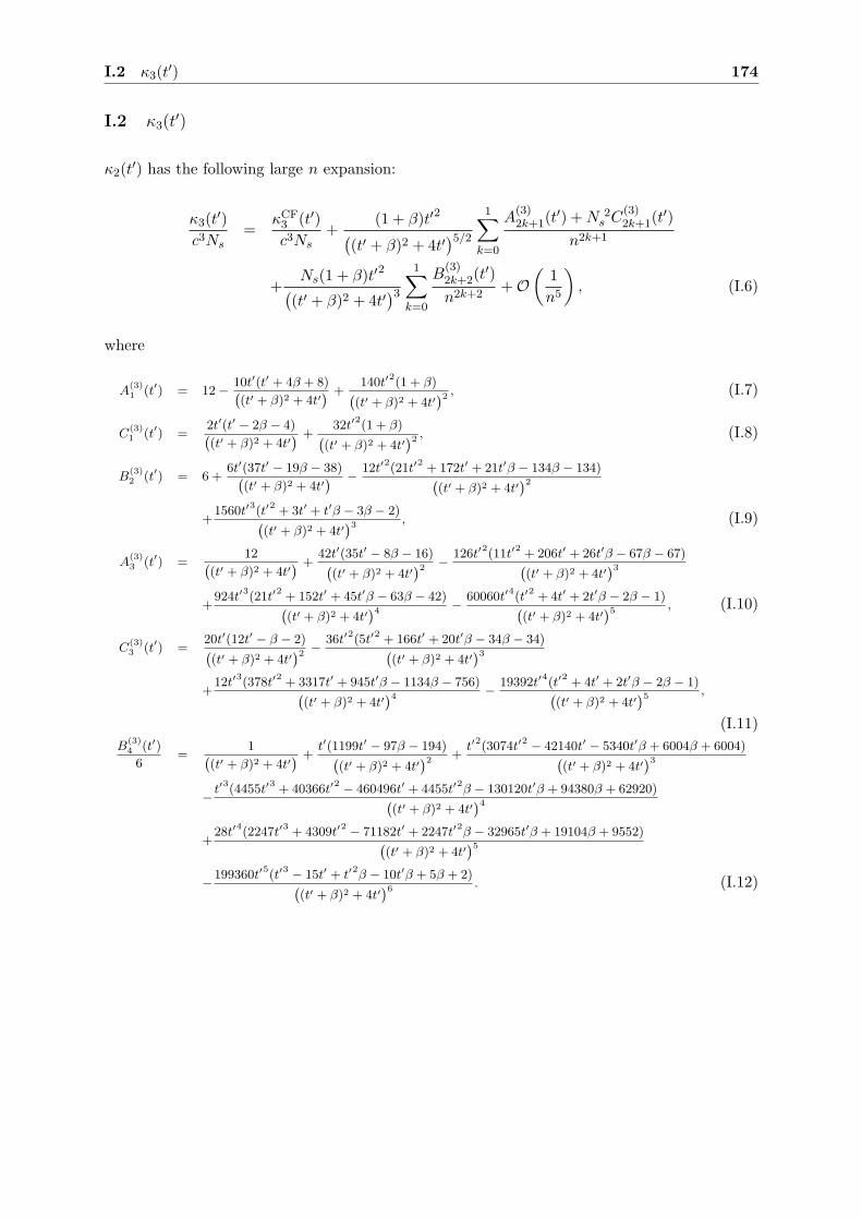
I.2 κ3(t′) 174

I.2 κ3(t′)

κ2(t′) has the following large n expansion:

κ3(t′)c3Ns

=κCF

3 (t′)c3Ns

+(1 + β)t′2

((t′ + β)2 + 4t′

)5/2

1∑

k=0

A(3)2k+1(t

′) +N 2s C

(3)2k+1(t

′)

n2k+1

+Ns(1 + β)t′2

((t′ + β)2 + 4t′

)3

1∑

k=0

B(3)2k+2(t

′)

n2k+2+ O

(1n5

)

, (I.6)

where

A(3)1 (t′) = 12 −

10t′(t′ + 4β + 8)((t′ + β)2 + 4t′

) +140t′

2(1 + β)

((t′ + β)2 + 4t′

)2 , (I.7)

C(3)1 (t′) =

2t′(t′ − 2β − 4)((t′ + β)2 + 4t′

) +32t′

2(1 + β)

((t′ + β)2 + 4t′

)2 , (I.8)

B(3)2 (t′) = 6 +

6t′(37t′ − 19β − 38)((t′ + β)2 + 4t′

) −12t′

2(21t′

2+ 172t′ + 21t′β − 134β − 134)((t′ + β)2 + 4t′

)2

+1560t′

3(t′

2+ 3t′ + t′β − 3β − 2)

((t′ + β)2 + 4t′

)3 , (I.9)

A(3)3 (t′) =

12((t′ + β)2 + 4t′

) +42t′(35t′ − 8β − 16)((t′ + β)2 + 4t′

)2 −126t′

2(11t′

2+ 206t′ + 26t′β − 67β − 67)((t′ + β)2 + 4t′

)3

+924t′

3(21t′

2+ 152t′ + 45t′β − 63β − 42)((t′ + β)2 + 4t′

)4 −60060t′

4(t′

2+ 4t′ + 2t′β − 2β − 1)

((t′ + β)2 + 4t′

)5 , (I.10)

C(3)3 (t′) =

20t′(12t′ − β − 2)((t′ + β)2 + 4t′

)2 −36t′

2(5t′

2+ 166t′ + 20t′β − 34β − 34)((t′ + β)2 + 4t′

)3

+12t′

3(378t′

2+ 3317t′ + 945t′β − 1134β − 756)((t′ + β)2 + 4t′

)4 −19392t′

4(t′

2+ 4t′ + 2t′β − 2β − 1)

((t′ + β)2 + 4t′

)5 ,

(I.11)B

(3)4 (t′)

6=

1((t′ + β)2 + 4t′

) +t′(1199t′ − 97β − 194)((t′ + β)2 + 4t′

)2 +t′

2(3074t′

2 − 42140t′ − 5340t′β + 6004β + 6004)((t′ + β)2 + 4t′

)3

−t′

3(4455t′

3+ 40366t′

2 − 460496t′ + 4455t′2β − 130120t′β + 94380β + 62920)

((t′ + β)2 + 4t′

)4

+28t′

4(2247t′

3+ 4309t′

2 − 71182t′ + 2247t′2β − 32965t′β + 19104β + 9552)

((t′ + β)2 + 4t′

)5

−199360t′

5(t′

3 − 15t′ + t′2β − 10t′β + 5β + 2)

((t′ + β)2 + 4t′

)6 . (I.12)

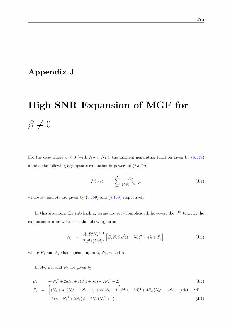
175

Appendix J

High SNR Expansion of MGF for

β 6= 0

For the case where β 6= 0 (with NR < ND), the moment generating function given by (5.139)

admits the following asymptotic expansion in powers of (γs)−1:

Mγ(s) =∞∑

`=0

A`(γs)nNs+`

, (J.1)

where A0 and A1 are given by (5.159) and (5.160) respectively.

In this situation, the sub-leading terms are very complicated, however, the jth term in the

expansion can be written in the following form:

Aj =A0R

jNsj+1

2(j!) (λβ2)j

[EjNsβ

√(1 + λβ)2 + 4λ+ Fj

], (J.2)

where Ej and Fj also depends upon λ, Ns, n and β.

In A2, E2, and F2 are given by

E2 = −(Ns2 + 2nNs + 1)β(1 + λβ) − 2Ns

2 − 2, (J.3)

F2 =

[

(Ns + n)(Ns

2 + nNs + 1)

+ n(nNs + 1)

]

β2(1 + λβ)2 + 4Ns

(Ns

2 + nNs + 1)β(1 + λβ)

+2(n−Ns

3 + 2Ns

)β + 2Ns

(Ns

2 + 4). (J.4)

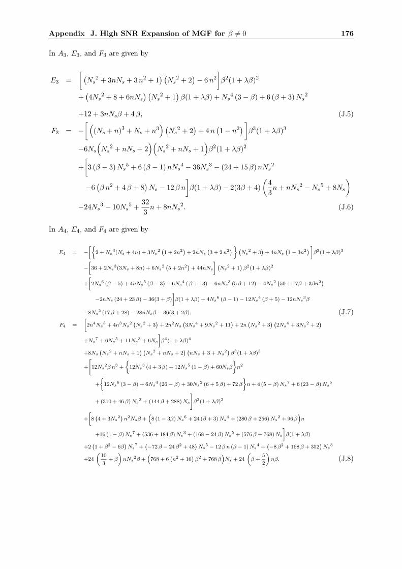
Appendix J. High SNR Expansion of MGF for β 6= 0 176

In A3, E3, and F3 are given by

E3 =

[(Ns

2 + 3nNs + 3n2 + 1) (Ns

2 + 2)− 6n2

]

β2(1 + λβ)2

+(4Ns

2 + 8 + 6nNs

) (Ns

2 + 1)β(1 + λβ) +Ns

4 (3 − β) + 6 (β + 3)Ns2

+12 + 3nNsβ + 4β, (J.5)

F3 = −

[((Ns + n)3 +Ns + n3

) (Ns

2 + 2)

+ 4n(1 − n2

)]

β3(1 + λβ)3

−6Ns

(Ns

2 + nNs + 2)(Ns

2 + nNs + 1)β2(1 + λβ)2

+

[

3 (β − 3)Ns5 + 6 (β − 1)nNs

4 − 36Ns3 − (24 + 15 β)nNs

2

−6(β n2 + 4β + 8

)Ns − 12β n

]

β(1 + λβ) − 2(3β + 4)

(43n+ nNs

2 −Ns5 + 8Ns

)

−24Ns3 − 10Ns

5 +323n+ 8nNs

2. (J.6)

In A4, E4, and F4 are given by

E4 = −[{

2 +Ns3(Ns + 4n) + 3Ns

2(1 + 2n2

)+ 2nNs

(3 + 2n2

)}(Ns

2 + 3)

+ 4nNs(1 − 3n2

)]β3(1 + λβ)3

−[36 + 2Ns

3(3Ns + 8n) + 6Ns2(5 + 2n2

)+ 44nNs

](Ns

2 + 1)β2(1 + λβ)2

+

[2Ns

6 (β − 5) + 4nNs5 (β − 3) − 6Ns

4 (β + 13) − 6nNs3 (5β + 12) − 4Ns

2(50 + 17β + 3βn2

)

−2nNs (24 + 23 β) − 36(3 + β)

]β(1 + λβ) + 4Ns

6 (β − 1) − 12Ns4 (β + 5) − 12nNs

3β

−8Ns2 (17 β + 28) − 28nNsβ − 36(3 + 2β), (J.7)

F4 =

[2n4Ns

3 + 4n3Ns2(Ns

2 + 3)

+ 2n2Ns(3Ns

4 + 9Ns2 + 11

)+ 2n

(Ns

2 + 3) (

2Ns4 + 3Ns

2 + 2)

+Ns7 + 6Ns

5 + 11Ns3 + 6Ns

]β4(1 + λβ)4

+8Ns(Ns

2 + nNs + 1) (Ns

2 + nNs + 2) (nNs + 3 +Ns

2)β3(1 + λβ)3

+

[

12Ns2β n3 +

{12Ns

3 (4 + 3 β) + 12Ns5 (1 − β) + 60Nsβ

}n2

+

{12Ns

6 (3 − β) + 6Ns4 (26 − β) + 30Ns

2 (6 + 5 β) + 72 β

}n+ 4 (5 − β)Ns

7 + 6 (23 − β)Ns5

+(310 + 46 β)Ns3 + (144 β + 288)Ns

]

β2(1 + λβ)2

+

[8(4 + 3Ns

2)n2Nsβ +

(8 (1 − 3β)Ns

6 + 24 (β + 3)Ns4 + (280 β + 256)Ns

2 + 96 β)n

+16 (1 − β)Ns7 + (536 + 184 β)Ns

3 + (168 − 24β)Ns5 + (576 β + 768)Ns

]β(1 + λβ)

+2(1 + β2 − 6β

)Ns

7 +(−72β − 24β2 + 48

)Ns

5 − 12β n (β − 1)Ns4 +

(−8β2 + 168 β + 352

)Ns

3

+24

(10

3+ β

)nNs

2β +(768 + 6

(n2 + 16

)β2 + 768 β

)Ns + 24

(β +

5

2

)nβ. (J.8)

177

References

[1] M. Abramowitz and I. A. Stegun, Handbook of mathematical functions with formulas,

graphs, and mathematical tables , vol. 55 of National Bureau of Standards Applied Math-

ematics Series . For sale by the Superintendent of Documents, U.S. Government Printing

Office, Washington, D.C. (1964).

[2] M. Adler, T. Shiota, and P. van Moerbeke, Random matrices, vertex operators and the

Virasoro algebra. Phys. Lett. A, 208, (1995) 67–78.

[3] M. Adler and P. van Moerbeke, Matrix integrals, Toda symmetries, Virasoro constraints,

and orthogonal polynomials. Duke Math. J., 80, (1995) 863–911.

[4] M. Adler and P. van Moerbeke, Hermitian, symmetric and symplectic random ensembles:

PDEs for the distribution of the spectrum. Ann. of Math. (2), 153, (2001) 149–189.

[5] E. W. Barnes, The theory of the G-function. Quart. J. Math., 31, (1899) 264–314.

[6] E. L. Basor and Y. Chen, Perturbed Hankel Determinants. J. Phys. A, 38, (2005) 10101–

10106.

[7] E. L. Basor and Y. Chen, Painleve V and the distribution function of a discontinuous

linear statistic in the Laguerre unitary ensembles. J. Phys. A, 42, (2009) 035203, 18.

[8] E. L. Basor, Y. Chen, and T. Ehrhardt, Painleve V and time-dependent Jacobi polyno-

mials. J. Phys. A, 43, (2010) 015204, 25.

[9] E. L. Basor, Y. Chen, and N. Mekareeya, The Hilbert series of N = 1SO(Nc) and Sp(Nc)

SQCD, Painleve VI and integrable systems. Nuclear Phys. B , 860, (2012) 421–463.

[10] E. L. Basor, Y. Chen, and H. Widom, Determinants of Hankel matrices. J. Funct. Anal.,

179, (2001) 214–234.

REFERENCES 178

[11] E. L. Basor, Y. Chen, and H. Widom, Hankel determinants as Fredholm determinants.

Random matrix models and their applications , vol. 40 of Math. Sci. Res. Inst. Publ.,

Cambridge Univ. Press, Cambridge, pp. 21–29 (2001).

[12] E. L. Basor, Y. Chen, and L. Zhang, PDEs satisfied by extreme eigenvalues distributions

of GUE and LUE. Random Matrices Theory Appl., 1, (2012) 1150003–1–1150003–21.

[13] W. C. Bauldry, Estimates of asymmetric Freud polynomials on the real line. J. Approx.

Theory , 63, (1990) 225–237.

[14] O. Bohigas, M.-J. Giannoni, and C. Schmit, Characterization of chaotic quantum spectra

and universality of level fluctuation laws. Phys. Rev. Lett., 52, (1984) 1–4.

[15] S. S. Bonan and D. S. Clark, Estimates of the Orthogonal Polynomials with Weight

exp(−xm), m an Even Positive Integer. J. Approx. Theory , 46, (1986) 408–410.

[16] S. S. Bonan and D. S. Clark, Estimates of the Hermite and the Freud polynomials. J.

Approx. Theory , 63, (1990) 210–224.

[17] S. S. Bonan, D. S. Lubinsky, and P. Nevai, Orthogonal polynomials and their derivatives.

II. SIAM J. Math. Anal., 18, (1987) 1163–1176.

[18] S. S. Bonan and P. Nevai, Orthogonal polynomials and their derivatives. I. J. Approx.

Theory , 40, (1984) 134–147.

[19] M. Buttiker, Scattering theory of thermal and excess noise in open conductors. Phys. Rev.

Lett., 65, (1990) 2901–2904.

[20] Y. Chen and M. V. Feigin, Painleve IV and degenerate Gaussian unitary ensembles. J.

Phys. A, 39, (2006) 12381–12393.

[21] Y. Chen, N. S. Haq, and M. R. McKay, Random matrix models, double-time Painleve

equations, and wireless relaying. J. Math. Phys., 54, 063506.

[22] Y. Chen and M. E. H. Ismail, Ladder operators and differential equations for orthogonal

polynomials. J. Phys. A, 30, (1997) 7817–7829.

[23] Y. Chen and M. E. H. Ismail, Thermodynamic relations of the Hermitian matrix ensem-

bles. J. Phys. A, 30, (1997) 6633–6654.

REFERENCES 179

[24] Y. Chen and M. E. H. Ismail, Jacobi polynomials from compatibility conditions. Proc.

Amer. Math. Soc., 133, (2005) 465–472 (electronic).

[25] Y. Chen, M. E. H. Ismail, and W. Van Assche, Tau-Function Constructions of the Recur-

rence Coefficients of Orthogonal Polynomials. Adv. in Appl. Math., 20, (1998) 141–168.

[26] Y. Chen and A. R. Its, Painleve III and a singular linear statistics in Hermitian random

matrix ensembles. I. J. Approx. Theory , 162, (2010) 270–297.

[27] Y. Chen and N. D. Lawrence, On the linear statistics of Hermitian random matrices. J.

Phys. A, 31, (1998) 1141–1152.

[28] Y. Chen and S. M. Manning, Distribution of linear statistics in random matrix models

(metallic conductance fluctuations). J. Phys.: Condens. Matter , 6, (1994) 3039–3044.

[29] Y. Chen and M. R. McKay, Coulumb fluid, Painleve transcendents, and the information

theory of MIMO systems. IEEE Trans. Inform. Theory , 58, (2012) 4594–4634.

[30] Y. Chen and G. Pruessner, Orthogonal polynomials with discontinuous weights. J. Phys.

A, 38, (2005) L191–L198.

[31] Y. Chen and L. Zhang, Painleve VI and the unitary Jacobi ensembles. Stud. Appl. Math.,

125, (2010) 91–112.

[32] T. S. Chihara, An Introduction to Orthogonal Polynomials . Gordon and Breach Science

Publishers, New York, mathematics and its Applications, Vol. 13 (1978).

[33] P. A. Clarkson, Painleve equations—Nonlinear Special Functions. Orthogonal polynomials

and special functions , vol. 1883 of Lecture Notes in Math., Springer, Berlin, pp. 331–411

(2006).

[34] C. M. Cosgrove, Chazy Classes IX–XI of Third-Order Differential Equations. Stud. Appl.

Math., 104, (2000) 171–228.

[35] C. M. Cosgrove and G. Scoufis, Painleve Classification of a Class of Differential Equations

of the Second Order and Second Degree. Stud. Appl. Math., 88, (1993) 25–87.

[36] D. Dai and L. Zhang, Painleve VI and Hankel determinants for the generalized Jacobi

weight. J. Phys. A, 43, (2010) 055207, 14.

REFERENCES 180

[37] P. A. Deift, Orthogonal polynomials and random matrices: a Riemann-Hilbert approach ,

vol. 3 of Courant Lecture Notes in Mathematics . New York University Courant Institute

of Mathematical Sciences, New York (1999).

[38] P. A. Deift, A. R. Its, and I. Krasovsky, Asymptotics of Toeplitz, Hankel, and

Toeplitz+Hankel determinants with Fisher-Hartwig singularities. Ann. of Math. (2), 174,

(2011) 1243–1299.

[39] P. A. Deift, A. R. Its, and X. Zhou, A Riemann-Hilbert approach to asymptotic prob-

lems arising in the theory of random matrix models, and also in the theory of integrable

statistical mechanics. Ann. of Math. (2), 146, (1997) 149–235.

[40] P. A. Deift and X. Zhou, A steepest descent method for oscillatory Riemann-Hilbert

problems. Bull. Amer. Math. Soc. (N.S.), 26, (1992) 119–123.

[41] P. A. Deift and X. Zhou, A steepest descent method for oscillatory Riemann-Hilbert

problems. Asymptotics for the MKdV equation. Ann. of Math. (2), 137, (1993) 295–368.

[42] P. A. Deift and X. Zhou, Asymptotics for the Painleve II Equation. Comm. Pure Appl.

Math., 48, (1995) 277–337.

[43] J. W. Demmel, The Probability That A Numerical Analysis Problem Is Difficult. Math.

Comp., 50, (1988) 449–480.

[44] P. Dharmawansa, M. R. McKay, and R. K. Mallik, Analytical performance of amplify-and-

forward MIMO relaying with orthogonal space-time block codes. IEEE Trans. Commun.,

58, (2010) 2147–2158.

[45] P. Diaconis, Group Representations in Probability and Statistics. Lect. Notes Monogr.

Ser., 11, (1988) i–192.

[46] F. J. Dyson, Statistical theory of the energy levels of complex systems. I. J. Mathematical

Phys., 3, (1962) 140–156.

[47] F. J. Dyson, Statistical theory of the energy levels of complex systems. II. J. Mathematical

Phys., 3, (1962) 157–165.

[48] F. J. Dyson, Statistical theory of the energy levels of complex systems. III. J. Mathematical

Phys., 3, (1962) 166–175.

REFERENCES 181

[49] A. Edelman, On the distribution of a scaled condition number. Math. Comp., 58, (1992)

185–190.

[50] Y. Fan and J. Thompson, MIMO Configurations for Relay Channels: Theory and Practice.

IEEE Trans. Wireless Commun., 6, (2007) 1774–1786.

[51] A. S. Fokas, A. R. Its, and A. V. Kitaev, The Isomonodromy Approach to Matrix Models

in 2D Quantum Gravity. Comm. Math. Phys., 147, (1992) 395–430.

[52] P. J. Forrester and C. M. Ormerod, Differential equations for deformed Laguerre polyno-

mials. J. Approx. Theory , 162, (2010) 653–677.

[53] F. D. Gakhov, Boundary value problems . Dover Publications Inc., New York, translated

from the Russian, Reprint of the 1966 translation (1990).

[54] B. Gambier, Sur les equations differentielles du second ordre et du premier degre dont

l’integrale generale est a points critiques fixes. Acta Math., 33, (1910) 1–55.

[55] I. P. Goulden and D. M. Jackson, Maps in locally orientable surfaces and integrals over

real symmetric surfaces. Canad. J. Math., 49, (1997) 865–882.

[56] I. S. Gradshteyn and I. M. Ryzhik, Table of integrals, series, and products . Else-

vier/Academic Press, Amsterdam, seventh edn., translated from the Russian, Translation

edited and with a preface by Alan Jeffrey and Daniel Zwillinger, With one CD-ROM

(Windows, Macintosh and UNIX) (2007).

[57] V. I. Gromak, I. Laine, and S. Shimomura, Painleve differential equations in the complex

plane, vol. 28 of de Gruyter Studies in Mathematics . Walter de Gruyter & Co., Berlin

(2002).

[58] P. J. Hanlon, R. P. Stanley, and J. R. Stembridge, Some combinatorial aspects of the

spectra of normally distributed random matrices. Hypergeometric functions on domains

of positivity, Jack polynomials, and applications (Tampa, FL, 1991) , vol. 138 of Contemp.

Math., Amer. Math. Soc., Providence, RI, pp. 151–174 (1992).

[59] E. Heine, Handbuch der Kugelfunktionen: Theorie und anwendungen, vols. I and II . G.

Reimer (1878).

[60] P. L. Hsu, On the distribution of roots of certain determinantal equations. Ann. Eugenics ,

9, (1939) 250–258.

REFERENCES 182

[61] M. E. H. Ismail and W.-X. Ma, Equations of motion for zeros of orthogonal polynomials

related to the Toda lattices. Arab J. Math. Sci., 17, (2011) 1–10.

[62] H. Jafarkhani, Space-time coding: theory and practice . Cambridge University Press (2005).

[63] M. Jimbo and T. Miwa, Monodromy preserving deformation of linear ordinary differential

equations with rational coefficients. II. Phys. D , 2, (1981) 407–448.

[64] M. Jimbo, T. Miwa, Y. Mori, and M. Sato, Density matrix of an impenetrable Bose gas

and the fifth Painleve transcendent. Phys. D , 1, (1980) 80–158.

[65] M. Jimbo, T. Miwa, and K. Ueno, Monodromy preserving deformation of linear ordinary

differential equations with rational coefficients. I. General theory and τ -function. Phys.

D , 2, (1981) 306–352.

[66] G. Karagiannidis, D. Zogas, and S. Kotsopoulos, Statistical properties of the EGC output

SNR over correlated Nakagami-m fading channels. IEEE Trans. Wireless Commun., 3,

(2004) 1764–1769.

[67] P. Kazakopoulos, P. Mertikopoulos, A. L. Moustakas, and G. Caire, Living at the edge:

a large deviations approach to the outage MIMO capacity. IEEE Trans. Inform. Theory ,

57, (2011) 1984–2007.

[68] R. Koekoek, P. A. Lesky, and R. F. Swarttouw, Hypergeometric orthogonal polynomials

and their q-analogues . Springer Monographs in Mathematics, Springer-Verlag, Berlin,

with a foreword by Tom H. Koornwinder (2010).

[69] A. B. J. Kuijlaars, K. T.-R. McLaughlin, W. Van Assche, and M. Vanlessen, The Riemann-

Hilbert approach to strong asymptotics for orthogonal polynomials on [−1, 1]. Adv. Math.,

188, (2004) 337–398.

[70] J. N. Laneman, D. N. C. Tse, and G. W. Wornell, Cooperative Diversity in Wireless

Networks: Efficient Protocols and Outage Behavior. IEEE Trans. Inform. Theory , 50,

(2004) 3062–3080.

[71] J. N. Laneman and G. W. Wornell, Distributed Space–Time-Coded Protocols for Ex-

ploiting Cooperative Diversity in Wireless Networks. IEEE Trans. Inform. Theory , 49,

(2003) 2415–2425, special issue on space-time transmission, reception, coding and signal

processing.

REFERENCES 183

[72] S. Li, M. McKay, and Y. Chen, On the Distribution of MIMO Mutual Information:

An In-Depth Painleve-Based Characterization. IEEE Trans. Inform. Theory , 59, (2013)

5271–5296.

[73] A. P. Magnus, Painleve-type differential equations for the recurrence coefficients of semi-

classical orthogonal polynomials. J. Comput. Appl. Math., 57, (1995) 215–237.

[74] V. A. Marcenko and L. A. Pastur, Distribution of eigenvalues in certain sets of random

matrices. Math. USSR Sb., 1, (1967) 457–483.

[75] M. R. McKay, A. Zanella, I. Collings, and M. Chiani, Error Probability and SINR Analysis

of Optimum Combining in Rician Fading. IEEE Trans. Commun., 57, (2009) 676–687.

[76] M. L. Mehta, Random matrices , vol. 142 of Pure and Applied Mathematics (Amsterdam) .

Elsevier/Academic Press, Amsterdam, third edn. (2004).

[77] H. N. Mhaskar, Bounds for certain Freud-type orthogonal polynomials. J. Approx. Theory ,

63, (1990) 238–254.

[78] H. L. Montgomery, The pair correlation of zeros of the zeta function. Analytic number

theory (Proc. Sympos. Pure Math., Vol. XXIV, St. Louis Univ., St. Louis, Mo., 1972) ,

Amer. Math. Soc., Providence, R.I., pp. 181–193 (1973).

[79] A. L. Moustakas, H. U. Baranger, L. Balents, A. M. Sengupta, and S. H. Simon, Com-

munication Through a Diffusive Medium: Coherence and Capacity. Science, 287, (2000)

287–290.

[80] K. A. Muttalib and Y. Chen, Distribution function for shot noise in Wigner-Dyson en-

sembles. Internat. J. Modern Phys. B , 10, (1996) 1999–2006.

[81] R. U. Nabar, H. Bolcskei, and F. W. Kneubuhler, Fading Relay Channels: Performance

Limits and Space–Time Signal Design. IEEE J. Sel. Areas Commun., 22, (2004) 1099–

1109.

[82] A. F. Nikiforov and V. B. Uvarov, Special functions of mathematical physics . Birkhauser

Verlag, Basel, a unified introduction with applications, Translated from the Russian and

with a preface by Ralph P. Boas, With a foreword by A. A. Samarskiı (1988).

[83] K. Okamoto, Polynomial Hamiltonians associated with Painleve Equations. I. Proc. Japan

Acad. Ser. A Math. Sci., 56, (1980) 264–268.

REFERENCES 184

[84] K. Okamoto, Polynomial Hamiltonians associated with Painleve Equations. II. Differential

equations satisfied by polynomial Hamiltonians. Proc. Japan Acad. Ser. A Math. Sci., 56,

(1980) 367–371.

[85] K. Okamoto, On the τ -function of the Painleve equations. Phys. D , 2, (1981) 525–535.

[86] V. A. Osipov and E. Kanzieper, Statistics of thermal to shot noise crossover in chaotic

cavities. J. Phys. A, 42, (2009) 475101, 14.

[87] V. A. Osipov and E. Kanzieper, Correlations of RMT Characteristic Polynomials and

Integrability: Hermitean Matrices. Ann. Physics , 325, (2010) 2251–2306.

[88] P. Painleve, Lecons, sur la theorie analytique des equations differentielles: professees a

Stockholm 1895 . A. Hermann (1897).

[89] M. Potters, J.-P. Bouchaud, and L. Laloux, Financial applications of random matrix

theory: old laces and new pieces. Acta Phys. Polon. B , 36, (2005) 2767–2784.

[90] C. J. Rees, Elliptic Orthogonal Polynomials. Duke Math. J., 12, (1945) 173–187.

[91] M. O. Searcoid, Metric spaces . Springer (2006).

[92] A. Selberg, Remarks on a multiple integral. Norsk Mat. Tidsskr., 26, (1944) 71–78.

[93] A. Sendonaris, E. Erkip, and B. Aazhang, User Cooperation Diversity–Part I: System

Description. IEEE Trans. Commun., 51, (2003) 1927–1938.

[94] A. Sendonaris, E. Erkip, and B. Aazhang, User Cooperation Diversity–Part II: Implemen-

tation Aspects and Performance Analysis. IEEE Trans. Commun., 51, (2003) 1939–1948.

[95] J. Shohat, A differential equation for orthogonal polynomials. Duke Math. J., 5, (1939)

401–417.

[96] M. Simon and M. Alouini, Digital Communication over Fading Channels , vol. 86. John

Wiley & Sons, Inc. (2005).

[97] K. Sogo, Time-dependent orthogonal polynomials and theory of soliton. Applications to

matrix model, vertex model and level statistics. J. Phys. Soc. Japan , 62, (1993) 1887–

1894.

REFERENCES 185

[98] Y. Song, H. Shin, and E. Hong, MIMO cooperative diversity with scalar-gain amplify-

and-forward relaying. IEEE Trans. Commun., 57, (2009) 1932–1938.

[99] G. Strang, Introduction to Linear Algebra . Wellesley-Cambridge Press (2009).

[100] G. Szego, Orthogonal Polynomials . American Mathematical Society, New York, American

Mathematical Society Colloquium Publications, v. 23 (1939).

[101] G. Szego, Hankel forms. Am. Math. Soc. Transl. (2), 108, (1977) 1–36.

[102] C. A. Tracy and H. Widom, Fredholm Determinants, Differential Equations and Matrix

Models. Comm. Math. Phys., 163, (1994) 33–72.

[103] C. A. Tracy and H. Widom, Level-Spacing Distributions and the Airy Kernel. Comm.

Math. Phys., 159, (1994) 151–174.

[104] C. A. Tracy and H. Widom, Level Spacing Distributions and the Bessel Kernel. Comm.

Math. Phys., 161, (1994) 289–309.

[105] M. Tsuji, Potential theory in modern function theory . Maruzen Co. Ltd., Tokyo (1959).

[106] W. Van Assche, Discrete Painleve equations for recurrence coefficients of orthogonal poly-

nomials. Difference equations, special functions and orthogonal polynomials , World Sci.

Publ., Hackensack, NJ, pp. 687–725 (2007).

[107] Z. Wang and G. Giannakis, A simple and general parameterization quantifying perfor-

mance in fading channels. IEEE Trans. Commun., 51, (2003) 1389–1398.

[108] E. P. Wigner, Statistical properties of real symmetric matrices with many dimensions .

Princeton University (1959).

[109] E. P. Wigner and P. Dirac, On the statistical distribution of the widths and spacings of

nuclear resonance levels. Proc. Cambridge Philo. Soc , vol. 47, Cambridge Univ Press, pp.

790–798 (1951).

[110] J. Wishart, The Generalised Product Moment Distribution in Samples from a Normal

Multivariate Population. Biometrika , 20A, (1928) 32–52.