orphan ides & williams (2007)

8/3/2019 Orphan Ides & Williams (2007)

http://slidepdf.com/reader/full/orphan-ides-williams-2007 1/53

Banco Central de ChileDocumentos de Trabajo

Central Bank of ChileWorking Papers

N° 398

Diciembre 2006

INFLATION TARGETING UNDER IMPERFECTKNOWLEDGE

Athanasios Orphanides John C. Williams

La serie de Documentos de Trabajo en versión PDF puede obtenerse gratis en la dirección electrónica:http://www.bcentral.cl/esp/estpub/estudios/dtbc. Existe la posibilidad de solicitar una copia impresa conun costo de $500 si es dentro de Chile y US$12 si es para fuera de Chile. Las solicitudes se pueden hacer porfax: (56-2) 6702231 o a través de correo electrónico:[email protected] .

Working Papers in PDF format can be downloaded free of charge from:http://www.bcentral.cl/eng/stdpub/studies/workingpaper. Printed versions can be ordered individuallyfor US$12 per copy (for orders inside Chile the charge is Ch$500.) Orders can be placed by fax: (56-2) 6702231or e-mail: [email protected].



BANCO CENTRAL DE CHILE

CENTRAL BANK OF CHILE

La serie Documentos de Trabajo es una publicación del Banco Central de Chile que divulgalos trabajos de investigación económica realizados por profesionales de esta institución oencargados por ella a terceros. El objetivo de la serie es aportar al debate temas relevantes ypresentar nuevos enfoques en el análisis de los mismos. La difusión de los Documentos de

Trabajo sólo intenta facilitar el intercambio de ideas y dar a conocer investigaciones, concarácter preliminar, para su discusión y comentarios.

La publicación de los Documentos de Trabajo no está sujeta a la aprobación previa de losmiembros del Consejo del Banco Central de Chile. Tanto el contenido de los Documentos deTrabajo como también los análisis y conclusiones que de ellos se deriven, son de exclusivaresponsabilidad de su o sus autores y no reflejan necesariamente la opinión del Banco Centralde Chile o de sus Consejeros.

The Working Papers series of the Central Bank of Chile disseminates economic researchconducted by Central Bank staff or third parties under the sponsorship of the Bank. Thepurpose of the series is to contribute to the discussion of relevant issues and develop newanalytical or empirical approaches in their analyses. The only aim of the Working Papers is todisseminate preliminary research for its discussion and comments.

Publication of Working Papers is not subject to previous approval by the members of theBoard of the Central Bank. The views and conclusions presented in the papers are exclusivelythose of the author(s) and do not necessarily reflect the position of the Central Bank of Chileor of the Board members.

Documentos de Trabajo del Banco Central de ChileWorking Papers of the Central Bank of Chile

Agustinas 1180Teléfono: (56-2) 6702475; Fax: (56-2) 6702231



Documento de Trabajo Working Paper

N° 398 N° 398

INFLATION TARGETING UNDER IMPERFECTKNOWLEDGE

Athanasios Orphanides John C. WilliamsBoard of Governors of theFederal Reserve System

Federal Reserve Bank of San Francisco

Resumen Un principio central del esquema de metas de inflación es la importancia que se da a establecer y mantener bienancladas las expectativas inflacionarias. En este artículo revisamos el papel que juegan ciertos elementos clavesde dicho esquema para cumplir con este objetivo, en una economía en la que los agentes económicos tienen una

comprensión imperfecta del ámbito económico dentro del cual el público construye sus expectativas y laautoridad debe formular e implementar la política monetaria. Usando un modelo estimado de la economía deEstados Unidos, mostramos que ciertas reglas de política monetaria que funcionarían bien bajo el supuesto deexpectativas racionales, pierden gran parte de su eficacia cuando se introduce el conocimiento imperfecto.Luego examinamos el desempeño de una regla de política de fácil aplicación que incorpora tres característicasesenciales del esquema de metas de inflación: transparencia, compromiso de mantener la estabilidad de preciosy un monitoreo estricto de las expectativas de inflación, y encontramos que los tres juegan un rol importantepara asegurar su éxito. Nuestro análisis sugiere que las reglas de diferencia simple en el espíritu de KnutWicksell son excelentes para anclar las expectativas inflacionarias a la meta del banco central, y que al hacerlologran una mejor estabilización de la inflación y de la actividad económica en un ambiente de conocimientoimperfecto.

Abstract A central tenet of inflation targeting is that establishing and maintaining well-anchored inflation expectations areessential. In this paper, we reexamine the role of key elements of the inflation targeting framework towards thisend, in the context of an economy where economic agents have an imperfect understanding of themacroeconomic landscape within which the public forms expectations and policymakers must formulate andimplement monetary policy. Using an estimated model of the U.S. economy, we show that monetary policy rulesthat would perform well under the assumption of rational expectations can perform very poorly when weintroduce imperfect knowledge. We then examine the performance of an easily implemented policy rule thatincorporates three key characteristics of inflation targeting: transparency, commitment to maintaining pricestability, and close monitoring of inflation expectations, and find that all three play an important role in assuringits success. Our analysis suggests that simple difference rules in the spirit of Knut Wicksell excel at tetheringinflation expectations to the central bank’s goal and in so doing achieve superior stabilization of inflation andeconomic activity in an environment of imperfect knowledge.

_______________Paper presented for the Ninth Annual Conference, Banco Central de Chile, October 2005. We would like tothank Richard Dennis, Bill English, Ali Hakan Kara, Thomas Laubach, Nissan Liviatan, John Murray, andRodrigo Vergara for useful comments. The opinions expressed are those of the authors and do not necessarilyreflect the views of the Board of Governors of the Federal Reserve System or the management of the FederalReserve Bank of San Francisco.E-mails: [email protected]; [email protected]



INFLATION T ARGETING

UNDER IMPERFECT K NOWLEDGE

Athanasios Orphanides Board of Governors of the Federal Reserve System

John C. WilliamsFederal Reserve Bank of San Francisco

A central tenet of inflation targeting is that establishing and

maintaining well-anchored inflation expectations are essential.

Well-anchored expectations enable inflation-targeting central banks to

achieve stable output and employment in the short-run, while ensuring

price stability in the long-run. Three elements of inflation targeting

have been critically important for the successful implementation

of this framework.1 First and foremost is the announcement of an

explicit quantitative inflation target and the acknowledgment thatlow, stable inflation is the primary objective and responsibility of the

central bank. Second is the clear communication of the central bank’s

policy strategy and the rationale for its decisions, which enhances the

predictability of the central bank’s actions and its accountability to

the public. Third is a forward-looking policy orientation, characterized

by the vigilant monitoring of inflation expectations at both short-term

and longer-term horizons. Together, these elements provide a focal

point for inflation, facilitate the formation of the public’s inflation

expectations, and provide guidance on actions that may be neededto foster price stability.

We would like to thank Richard Dennis, Bill English, Ali Hakan Kara, ThomasLaubach, Nissan Liviatan, John Murray, and Rodrigo Vergara for useful comments.The opinions expressed are those of the authors and do not necessarily reflect the viewsof the Board of Governors of the Federal Reserve System or the management of theFederal Reserve Bank of San Francisco.

1. A number of studies have examined in detail the defining characteristics of

inflation targeting. See Leiderman and Svensson (1995); Bernanke and Mishkin (1997);Bernanke and others (1999); Goodfriend (2004).



2 Athanasios Orphanides and John C. Williams

Although inflation-targeting central banks stress these key

elements, the literature that studies inflation targeting in the

context of formal models largely describes inflation targeting interms of the solution to an optimization problem within the confines

of a linear rational expectations model. This approach is limited

in its appreciation of the special features of the inflation-targeting

framework, as emphasized by Faust and Henderson (2004), and it

strips inflation targeting of its raison d’être. In an environment of

rational expectations with perfect knowledge, for instance, inflation

expectations are anchored as long as policy satisfies a minimum test

of stability. Furthermore, with the possible exception of a one-time

statement of the central bank’s objectives, central bank communicationloses any independent role because the public already knows all it

needs in order to form expectations relevant for its decisions. In

such an environment, the public’s expectations of inflation and

other variables are characterized by a linear combination of lags of

observed macroeconomic variables, and, as such, they do not merit

special monitoring by the central bank or provide useful information

to the policymaker for guiding policy decisions.

In this paper, we argue that in order to understand the attraction

of inflation targeting to central bankers and its effectiveness relative toother monetary policy strategies, it is essential to recognize economic

agents’ imperfect understanding of the macroeconomic landscape

within which the public forms expectations and policymakers

formulate and implement monetary policy. To this end, we consider two

modest deviations from the perfect-knowledge rational expectations

benchmark, and we reexamine the role of the key elements of the

inflation-targeting framework in the context of an economy with

imperfect knowledge. We find that including these modifications

provides a rich framework in which to analyze inflation-targeting

strategies and their implementation.

The first relaxation of perfect knowledge that we incorporate is to

recognize that policymakers face uncertainty regarding the evolution

of key natural rates. In the United States, for example, estimates

of the natural interest and unemployment rates are remarkably

imprecise.2 This problem is arguably even more dramatic for small

2. For discussion and documentation of this imprecision, see Orphanides andWilliams (2002); Laubach and Williams (2003); Clark and Kozicki (2005). See also



3Inflation Targeting under Imperfect Knowledge

open economies and transitional economies that have tended to adopt

inflation targeting. Policymakers’ misperceptions on the evolution

of natural rates can result in persistent policy errors, hinderingsuccessful stabilization policy.3

Our second modification is to allow for the presence of imperfections

in expectations formation that arise when economic agents have

incomplete knowledge of the economy’s structure. We assume that agents

rely on an adaptive learning technology to update their beliefs and form

expectations based on incoming data. Recent research highlights the

ways in which imperfect knowledge can act as a propagation mechanism

for macroeconomic disturbances in terms of amplification and persistence

that have first-order implications for monetary policy.4 Agents may relyon a learning technology to guard against numerous potential sources

of uncertainty. One source could be the evolution of natural rates in the

economy, paralleling the uncertainty faced by policymakers. Another

might involve the policymakers’ understanding of the economy, their

likely response to economic developments, and the precise quantification

of policy objectives. Recognition of this latter element in the economy

highlights a role for central bank communications, including that of

an explicit quantitative inflation target, which would be absent in an

environment of perfect knowledge.We investigate the role of inflation targeting in an environment of

imperfect knowledge using an estimated quarterly model of the U.S.

economy. Specifically, we compare the performance of the economy

subject to shocks with characteristics similar to those observed in

the data over the past four decades under alternative informational

assumptions and policy strategies. Following McCallum (1988) and

Taylor (1993), we focus on implementable policy rules that capture the

key characteristics of inflation targeting. Our analysis shows that some

monetary policy rules that would perform well under the assumption

of rational expectations with perfect knowledge perform very poorly

when we introduce imperfect knowledge. In particular, rules that

rely on estimates of natural rates for setting policy are susceptible

to persistent errors. Under certain conditions, these errors can give

rise to endogenous inflation scares, whereby inflation expectations

become unmoored from the central bank’s desired anchor. These

3. For analyses of the implications of misperceptions for policy design, seeOrphanides and Williams (2002); Orphanides (2003b); Cukierman and Lippi (2005).




results illustrate the potential shortcomings of such standard policy

rules and the desirability of identifying an alternative monetary policy

framework when knowledge is imperfect.We then examine the performance of an easily implemented

policy rule that incorporates the three key characteristics of

inflation targeting highlighted above in an economy with imperfect

knowledge. The exercise reveals that all three play an important

role in ensuring success. First, central bank transparency, including

explicit communication of the inflation target, can lessen the burden

placed on agents to infer central bank intentions and can thereby

improve macroeconomic performance. Second, policies that do not

rely on estimates of natural rates are easy to communicate andare well designed for ensuring medium-run inflation control when

natural rates are highly uncertain. Finally, policies that respond to

the public’s near-term inflation expectations help the central bank

avoid falling behind the curve in terms of controlling inflation, and

they result in better stabilization outcomes than policies that rely

only on past realizations of data and ignore information contained in

private agents’ expectations.

A reassuring aspect of our analysis is that despite the environment

of imperfect knowledge and the associated complexity of the economicenvironment, successful policy can be remarkably simple to implement

and communicate. We find that simple difference rules that do not

require any knowledge of the economy’s natural rates are particularly

well suited to ensure medium-run inflation control when natural rates

are highly uncertain. These rules share commonalities with the simple

robust strategy first proposed by Wicksell (1936 [1898]), who, after

defining the natural interest rate, pointed out that precise knowledge

about it, though desirable, was neither feasible nor necessary for policy

implementation aimed toward maintaining price stability.

This does not mean that the bank ought actually to ascertain the

natural rate before fixing their own rates of interest. That would,

of course, be impracticable, and would also be quite unnecessary.

For the current level of commodity prices provides a reliable test of

the agreement or diversion of the two rates. The procedure should

rather be simply as follows: So long as prices remain unchanged, the

bank’s rate of interest is to remain unaltered. If prices rise, the rate

of interest is to be raised; and if prices fall, the rate of interest is tobe lowered; and the rate of interest is henceforth to be maintained at

its new level until a further movement in prices calls for a further




In my opinion, the main cause of the instability of prices resides in

the instability of the banks to follow this rule.5

Our analysis confirms that simple difference rules that implicitly

target the price level in the spirit of Wicksell excel at tethering inflation

expectations to the central bank’s goal. In so doing, they achieve

superior stabilization of inflation and economic activity.

The remainder of the paper is organized as follows. Section 1

describes the estimated model of the economy. Section 2 lays out the

model of perpetual learning and its calibration. Section 3 analyzes

key features of the model under rational expectations and imperfect

knowledge. Section 4 examines the performance of alternativemonetary policy strategies, including our implementation of inflation

targeting. Section 5 concludes.

1. A SIMPLE ESTIMATED MODEL OF THE U.S. ECONOMY

We use a simple estimated quarterly model of the U.S. economy

from Orphanides and Williams (2002), the core of which consists of

the following two equations:

π φ π φ π α σπ π π π π πt te

t te

t t eu u e e= + −( ) + −( )+ ( )+ −1 121 0*

, , ,∼ iid ; (1)

u u u u u

r r e e

t u te

t t t

u ta

t u t u

= + + +

+ −( )+

+ − −

−

φ χ χ χ

α

1 1 1 2 2 3

1 0

*

*, , ,∼ iid σσeu

2( ).

(2)

Here π denotes the annualized percent change in the aggregate output

price deflator, u denotes the unemployment rate, u* denotes the (true)

natural rate of unemployment, r a denotes the (ex ante) real interest

rate with one-year maturity, and r * the (true) natural real rate of

interest. The superscript e denotes the public’s expectations formed

during t – 1. This model combines forward-looking elements of the new

synthesis model studied by Goodfriend and King (1997), Rotemberg

and Woodford (1999), Clarida, Galí, and Gertler (1999), and McCallum

and Nelson (1999), with intrinsic inflation and unemployment inertia

as in Fuhrer and Moore (1995b), Batini and Haldane (1999), Smets

(2003), and Woodford (2003).




The Phillips curve in this model (equation 1) relates inflation

in quarter t to lagged inflation, expected future inflation, and

expectations of the unemployment gap during the quarter, usingretrospective estimates of the natural rate discussed below. The

estimated parameter φπ measures the importance of expected inflation

for the determination of inflation. The unemployment equation

(equation 2) relates unemployment in quarter t to the expected future

unemployment rate, two lags of the unemployment rate, the natural

rate of unemployment, and the lagged real interest rate gap. Here, two

elements reflect forward-looking behavior: the estimated parameter φu,

which measures the importance of expected unemployment, and the

duration of the real interest rate, which serves as a summary of theinfluence of interest rates of various maturities on economic activity. We

restrict the coefficient χ3

to equal 1 – φu

– χ1

– χ2 so that the equation

can be equivalently written in terms of the unemployment gap.

In estimating this model, we face the difficulty that expected

inflation and unemployment are not directly observed. Instrumental

variable and full-information maximum likelihood methods impose the

restriction that the behavior of monetary policy and the formation of

expectations be constant over time, neither of which appears tenable

over the sample period that we consider (1969–2002). Instead, wefollow the approach of Roberts (1997) and use survey data as proxies

for expectations.6 In particular, we use the median forecasts from

the Survey of Professional Forecasters from the prior quarter as the

relevant expectations for determining inflation and unemployment

in period t; that is, we assume expectations are based on information

available at time t – 1. We also employ first-announced estimates of

these series in our estimation, to match the inflation and unemployment

data as well as possible with the forecasts. Our primary sources for

these data are the Real-Time Dataset for Macroeconomists and the

Survey of Professional Forecasters, both currently maintained by the

Federal Reserve Bank of Philadelphia (Zarnowitz and Braun, 1993;

Croushore, 1993; Croushore and Stark, 2001). Using least squares over

the sample 1969:1 to 2002:2, we obtain the following estimates:

π π πt te

t te

tu u e= + − −( )+( )

+−−( )

−( )

0 540 0 460 0 3410 086

1 10 099

. . .. .

*ππ,t

, (3)

SER = 1.38; DW = 2.09.




u u u ut t

e

t t= + − −

( )+

( )−

( )−

0 257 1 170 0 459 0 00 084

10 107

10 071

2. . . .. . .

332 0 0430 013

1−−( ) ( )

−+ −( )+u r r e

t t

a

t u t

*

.

*,. , (4)

SER = 0.30; DW = 2.08.

The numbers in parentheses are the estimated standard errors

of the corresponding regression coefficients; SER is the standard

error of the regression and DW is the Durbin-Watson statistic.

(Dashes are shown under the restricted parameters.) The estimated

unemployment equation also includes a constant term (not shown) that

captures the average premium of the one-year Treasury bill rate we

use for estimation over the average of the federal funds rate, which

corresponds to the natural interest rate estimates we employ in the

model. For simplicity, we do not model the evolution of risk premiums.

In the model simulations, we impose the expectations theory of the

term structure, whereby the one-year rate equals the expected average

of the federal funds rate over four quarters.

1.1 Natural Rates

We assume that the true processes governing natural rates in

the economy follow highly persistent autoregressions. Specifically,

we posit that the natural rates follow

u u u et t u t* * *

*,. .= + +−0 01 0 99 1 and

r r r et t r t* * *

*,. .= + +−0 01 0 99 1 ,

where u* and r * denote the unconditional means of the natural rates

of unemployment and interest, respectively. The assumption that

these processes are stationary is justified by the finding, based on a

standard augmented Dickey-Fuller ( ADF) test, that one can reject the

null hypothesis of nonstationarity of both the unemployment rate and

the ex post real federal funds rate over 1950–2003 at the 5 percent

level. To capture the assumed high persistence of these series, we set

the first-order autoregressive, or AR(1), coefficient to 0.99 and then

calibrate the innovation variances to be consistent with estimates of

time variation in the natural rates in postwar U.S. data.

As discussed in Orphanides and Williams (2002), estimates of the

variances of the innovations to the natural rates differ widely Indeed




U.S. data do not provide clear guidance regarding these parameters.

We therefore consider three alternative calibrations of these variances,

which we index by s. The case of s = 0 corresponds to constant and knownnatural rates, where σ σe eu r * *

= = 0 . For the case of s = 1, we assumeσeu*

= 0.070 and σer *= 0.085. These values imply an unconditional

standard deviation of the natural rate of unemployment (interest) of

0.50 (0.60), which is in the low end of the range of standard deviations

of smoothed estimates of these natural rates suggested by various

estimation methods (see Orphanides and Williams, 2002, for details).

Finally, the case of s = 2 corresponds to the high end of the range of

estimates; for this case we assume σeu*= 0.140 and σer *

= 0.170. The

relevant values of s for many small open economies and transitionaleconomies may be even higher than estimates based on U.S. data, given

the relative stability of the post-war U.S. economy.

1.2 Monetary Policy

We consider two classes of simple monetary policy rules. First, we

analyze versions of the Taylor rule (Taylor, 1993), where the level of

the nominal interest rate is determined by the perceived natural rate of

interest,r t * , the inflation rate, and a measure of the level of the perceived

unemployment gap (namely, the difference between the unemployment

rate and the perceived natural rate of unemployment, ut*):

i r u ut t t je

t je

u t ke

t= + + −( )+ −( )+ + +

* * *π θ π π θπ , (5)

where π denotes the four-quarter average of the inflation rate, π* is the

central bank’s inflation objective, j is the forecast horizon of inflation,

and k is the forecast horizon of the unemployment rate forecast. We

consider a range of values for the forecast horizons from –1, in whichcase policy responds to the latest observed data (for quarter t – 1), to

a forecast horizon up to three years into the future. When policy is

based on forecasts, we assume that the central bank uses the same

forecasts of inflation and the unemployment rate that are available

to private agents.

We refer to this class of rules as level rules because they relate

the level of the interest rate to the level of the unemployment gap.

Rules of this type have been found to perform quite well in terms

of stabilizing economic fluctuations, at least when the natural ratesof interest and unemployment are accurately measured. For our




the unemployment gap instead of the output gap, recognizing that the

two are related by Okun’s (1962) law. In his 1993 exposition, Taylor

examines response parameters equal to 0.5 for the inflation gap andthe output gap, which, with an Okun’s coefficient of 2.0, corresponds

to setting θπ = 0.5 and θu

= – 1.0.

If policy follows the level rule given by equation 5, then the

policy error introduced in period t by natural rate misperceptions

is given by

r r u ut t u t t

* * * *−

− −

θ.

Although unintentional, these errors could subsequently induceundesirable fluctuations in the economy, worsening stabilization

performance. The extent to which misperceptions regarding the

natural rates translate into policy-induced fluctuations depends on the

parameters of the policy rule. As is evident from the above expression,

policies that are relatively unresponsive to real-time assessments of the

unemployment gap—that is, those with small θu —minimize the impact

of misperceptions regarding the natural unemployment rate.

As discussed in Orphanides and Williams (2002), one policy

rule that is immune to natural rate mismeasurement of the kindconsidered here is a difference rule, in which the change in the nominal

interest rate is determined by the inflation rate and the change in the

unemployment rate:

∆ ∆∆i ut t je

u t k= −( )++ +θ π π θπ*

. (6)

This rule is closely related to price-level targeting strategies. It

corresponds to the first difference of the rule that would be obtained

if the price level were substituted for inflation in the level rule

(equation 5).7 This policy rule is as simple, in terms of the number of

parameters, as the original formulation of the Taylor rule. However,

the difference rule is simpler to communicate and implement in

practice than the Taylor rule because it does not require knowledge

of the natural rates of interest or unemployment. Policy guided by

a difference rule can thus be more transparent than policy guided

by a level rule.

7. For related policy rule specifications, see Judd and Motley (1992); Fuhrer andMoore (1995a); Orphanides (2003a). See also Orphanides and Williams (2002, 2005b)




2. PERPETUAL LEARNING

Expectations play a central role in determining inflation, theunemployment rate, and the interest rate in the model. We consider

two alternative models of expectations formation. One model, used

in most monetary policy research, is rational expectations, that is,

expectations that are consistent with the model. The second model

is one of perpetual learning, where agents continuously reestimate a

forecasting model and form expectations using that model.

In the case of learning, we follow Orphanides and Williams (2005c)

and posit that agents obtain forecasts for inflation, unemployment,

and interest rates by estimating a restricted vector autoregression

(VAR) corresponding to the reduced form of the rational expectations

equilibrium with constant natural rates. We assume that this VAR is

estimated recursively with constant-gain least squares.8 Each period,

agents use the resulting VAR to construct one-step-ahead and multi-

step-ahead forecasts. This learning model can be justified in two ways.

First, in practice agents are working with finite quantities of data, and

the assumption of rational expectations only holds in the distant future

when sufficient data have been collected. Alternatively, agents may allowfor the possibility of structural change and therefore place less weight

on older data, in which case learning is a never-ending process.

Specifically, let Yt denote the 1 x 3 vector consisting of the

inflation rate, the unemployment rate, and the federal funds rate,

each measured at time t: Yt = (π

t, u

t, i

t). Let X

t be the j x 1 vector of

a constant and lags of Yt that serve as regressors in the forecasting

model. The precise number of lags of elements of Yt that appear in

X t depends on the policy rule. For example, consider the difference

rule (equation 6) when policy responds to the three-quarter-aheadinflation forecast, j = 3, and the lagged change in the unemployment

rate, k = -1. (This is one of the policies for which we present detailed

simulation results later in the paper). In this case, two lags of the

unemployment rate and one lag each of inflation and the interest rate

suffice to capture the reduced-form dynamics under rational expectations

with constant natural rates, so X t = (1, π

t –1, u

t –1, u

t –2, i

t –1)′.

The recursive estimation can be described as follows: let ct be the

j x 3 vector of coefficients of the forecasting model. Then, using data




through period t, the parameters for the constant-gain least squares

forecasting model can be written as

c c R X Y X ct t t t t t t= + − ′( )−−

−11

1κ , and (7)

R R X Rt t t t t= + ′ −( )− −1 1κ X , (8)

where κ > 0 is a small constant gain.

This algorithm estimates all parameters of the agent’s forecasting

system and does not explicitly incorporate any information regarding

the central bank’s numerical inflation objective. Later, we introduce

this element of inflation targeting by positing that the announcementand explicit commitment to a quantitative inflation target simplifies

the agent’s forecasting problem by reducing by one the number of

parameters requiring estimation and updating.

A key parameter for the constant-gain-learning algorithm is the

updating rate, κ. To calibrate the relevant range for this parameter,

we examined how well different values of κ fit the expectations data

from the Survey of Professional Forecasters, following Orphanides

and Williams (2005c). To examine the fit of the Survey of Professional

Forecasters (SPF), we generated a time series of forecasts using arecursively estimated VAR for the inflation rate, the unemployment

rate, and the federal funds rate. In each quarter, we reestimated the

model using all historical data available during that quarter (generally

from 1948 through the most recent observation). We allowed for

discounting of past observations by using geometrically declining

weights. This procedure resulted in reasonably accurate forecasts of

inflation and unemployment, with root mean squared errors (RMSE)

comparable to the residual standard errors from the estimated

structural equations (equations 3 and 4). We found that discountingpast data with values for κ in the range of 0.01 to 0.04 yielded forecasts

closer to the SPF, on average, than the forecasts obtained with lower

or higher values of κ. Milani (2005) finds a similar range of values in

an estimated dynamic stochastic general-equilibrium (DSGE) model

with learning. In light of these results, we consider three alternative

calibrations of the gain: κ = {0.01, 0.02, 0.03}, with κ = 0.02 serving as

a baseline value.9 As in the case of natural rate variation, the relevant

values of κ may be higher for small open economies and transitional




economies than for the U.S. data, owing to the relative stability of the

post-war U.S. economy.

Given this calibration of the model, this learning mechanismrepresents a relatively modest deviation from rational expectations

and yields reasonable forecasts. Indeed, agents’ average forecasting

performance in the model is close to the optimal forecast.

2.1 Central Bank Learning

In the case of level rules, policymakers need a procedure to computereal-time estimates of the natural rates. If policymakers knew the true

data-generating processes governing the evolution of natural rates, theycould use this knowledge to design the optimal estimator. In practice,however, considerable uncertainty surrounds these processes, and theoptimal estimator for one process may perform poorly if the processis misspecified. Williams (2005) shows that a simple constant-gainmethod to update natural rate estimates based on the observed ratesof unemployment and (ex post) real interest rates is reasonably robustto natural rate model misspecification. We follow this approach andassume that policymakers update their estimates of natural rates using

simple constant-gain estimators given by the following equations:

r r i r t t t t t

* * *.= + − −

− − − −1 1 1 10 005 π , and

u u u ut t t t

* * *.= + −

− − −1 1 10 005 .

3. EFFECTS OF IMPERFECT KNOWLEDGE ON ECONOMIC

D YNAMICS

We first present some simple comparisons of the economy’s behaviorunder rational expectations with known natural rates and underlearning with time-varying and unobservable natural rates. Underlearning, the economy is governed by nonlinear dynamics, so we usenumerical simulations to illustrate the properties of the model economy,conditional on the policymaker following a specific policy rule.

3.1 Simulation Methodology

In the case of rational expectations with constant and known




numerically as described in Levin, Wieland, and Williams (1999). In all

other cases, we compute approximations of the unconditional moments

and impulse responses using simulations of the model.For model stochastic simulations used to compute estimates of

unconditional moments, the initial conditions for each simulation

are given by the rational expectations equilibrium with known andconstant natural rates. Specifically, all model variables are initializedto their steady-state values, assumed without loss of generality tobe zero. The central bank’s initial perceived levels of the natural

rates are set to their true values, likewise equal to zero. Finally, theinitial values of the c and R matrices describing the private agents’

forecasting model are initialized to their respective values, whichcorrespond to the reduced form of the rational equilibrium solution tothe structural model assuming constant and known natural rates.

Each period, innovations are generated from Gaussiandistributions, with variances reported above. The innovations are

serially and contemporaneously uncorrelated. For each period, thestructural model is simulated, the private agent’s forecasting modelis updated (resulting in a new set of forecasts), and the central bank’snatural rate estimate is updated. To estimate model moments, we

simulate the model for 41,000 periods and discard the first 1,000periods to mitigate the effects of initial conditions. We compute theunconditional moments from sample root mean squares from the

remaining 40,000 periods (10,000 years) of simulation data.10

Private agents’ learning process injects a nonlinear structure intothe model, which may generate explosive behavior in a stochasticsimulation of sufficient length for some policy rules that would have

been stable under rational expectations. One source of instabilitystems from the possibility that the forecasting model itself may

become unstable. We take the view that private forecasters rejectunstable models in practice. Each period of the simulation, we compute

the maximum modulus root of the forecasting VAR excluding theconstants. If the modulus of this root falls below the critical value of one, the forecasting model is updated as described above; if not, we

assume that the forecasting model is not updated and the c and R

matrices are held at their respective previous-period values.11

10. Simulations under rational expectations, in which we can compute the moments

directly, indicate that this sample size is sufficient to yield very accurate estimates of the unconditional variances. Testing further indicates that 1,000 periods are sufficientto remove the effects of initial conditions on simulated second moments.




Stability of the forecasting model is not sufficient to ensure

stability in all simulations. We therefore impose a second condition

that restrains explosive behavior. In particular, if the inflation rateor the unemployment gap exceeds, in absolute value, five times itsrespective unconditional standard deviation (computed under the

assumption of rational expectations and known and constant naturalrates), then the variable that exceeds this bound is constrained toequal the corresponding limit in that period. These constraints onthe model are sufficient to avoid explosive behavior for the exercises

that we consider in this paper; they are rarely invoked for most of thepolicy rules we study, particularly for optimized policy rules.

For impulse responses, we first compute an approximation of the steady-state distribution of the model state vector by running astochastic simulation of 100,000 periods. We then draw 1,001 samplestate vectors from this distribution and compute the impulse responsefunction for each of these draws. From these 1,001 impulse response

functions, we compute an estimate of the distribution of the modelimpulse response functions.

3.2 Impulse Responses

We use model impulse responses to illustrate the effects of learning

on macroeconomic dynamics. For this purpose, let monetary policy

follow a level policy rule similar to that proposed by Taylor (1993),

with θπ = 0.5 and θu

= –1, where the inflation forecast horizon is three

quarters ahead ( j = 3) and that of the unemployment rate is the last

observed quarter (that is, k = –1).Figure 1 compares the impulse responses of inflation, the nominal

interest rate, and the unemployment rate to one-standard-deviation

shocks to inflation and unemployment under perfect knowledge(that is, rational expectations with known natural rates) with thecorresponding impulse responses under imperfect knowledge withtime variation in the natural rates, s = 1, and perpetual learningwith gain κ = 0.02. Each period corresponds to one quarter. Under

learning, the impulse responses to a specific shock vary with thestate of the economy and the state of beliefs governing the formationof expectations. In other words, the responses vary with the initial

conditions, { X , c, R}, at the time the shock occurs. To summarize the

range of possible outcomes in the figure, we plot the median and the 70percent range of the distribution of impulse responses, correspondingto the stationary distribution of {X c R} Under rational expectations



Figure 1. Impulse Response Functions

under the Taylor Rulea

A. Inflation response B. Inflation responseto inflation shock to unemployment shock

C. Unemployment response D. Unemployment responseto inflation shock to unemployment shock

E. Interest rate response F. Interest rate responseto inflation shock to unemployment shock

Source: Authors' computations.

a. The Taylor rule is defined as i r u ut t te

te

t t= + + −

− −

+ + −

* * *

.π π π3 3 10 5 . The graphs display rational expectations with

perfect knowledge (RE), and median and 70 percent range of outcomes under learning with s = 1 and κ = 0.02




The dynamic impulse responses to a specific shock exhibit

considerable variation under learning. Furthermore, the distribution

of responses is not symmetric around the impulse response that obtainsunder rational expectations. For example, the impulse responses of

inflation and unemployment to an inflation shock are noticeably

skewed in a direction that yields greater persistence. This persistence

may be quite extreme with some probability, indicating that transitory

shocks can have very long-lasting effects under learning.

3.3 Macroeconomic Variability and Persistence

Perpetual learning provides a powerful propagation mechanismfor economic shocks in the economy, resulting in greater volatility

and persistence. We present a summary comparison of the asymptotic

variances and persistence for this experiment in table 1, which includes

the full range of natural range variation and values of κ considered

here. Learning on the part of the public increases the variability and

persistence of key macroeconomic variables. Even in the absence of

natural rate misperceptions (the case of s = 0), shocks to inflation and

unemployment engender time variation in private agents’ estimates of

the VAR used for forecasting. This time variation in the VAR coefficients

adds persistent noise to the economy relative to the perfect-knowledge

benchmark. As a result, the unconditional variances and the serial

correlations of inflation, unemployment, and the interest rate rise under

learning. These effects are larger for higher values of κ, for which the

sensitivity of the VAR coefficients to incoming data is greater.

The presence of natural rate variation amplifies the effects of

private sector learning on macroeconomic variability and persistence.

Under rational expectations and the Taylor rule, time-varying natural

rates and the associated misperceptions increase the variability

of inflation, but have relatively little effect on the variability

of the unemployment gap and interest rates. Nevertheless, the

combination of private sector learning and natural rate variation (and

misperceptions) can dramatically increase macroeconomic variability

and persistence. For example, under the Taylor rule, the standard

deviation of the unemployment gap rises from 0.87 percent under

rational expectations with constant natural rates to 1.11 percent

under learning with s = 1 andκ = 0.02. For inflation, the increase

in the standard deviation is even more dramatic, from 2.93 percent

to 4 35 percent The first-order autocorrelation of the unemployment



b l e 1 .

P e r f o r m a n c e u n d e r

t h e T a y l o r R u l e

S t a n d a r d d e v

i a t i o n

F i r s t - o r d e r a u t o c o r r e l a t i o n

p e c t a t i o n s

s

π

u – u *

∆ i

π

u – u *

i

t i o n a l

e x p e c t a t i o n s

0

2 .

9 3

0 . 8

7

2 .

3 3

0 . 8

1

0 . 8

8

0 . 7

8

1

3 .

2 2

0 . 8

8

2 .

3 5

0 . 8

4

0 . 8

8

0 . 8

2

2

3 .

9 4

0 . 8

9

2 .

3 9

0 . 8

9

0 . 8

8

0 . 8

9

0 .

0 1

0

3 .

2 9

0 . 9

3

2 .

5 7

0 . 8

4

0 . 8

9

0 . 8

1

1

4 .

1 6

1 . 1

0

2 .

8 9

0 . 8

9

0 . 9

2

0 . 8

6

2

5 .

0 0

1 . 2

2

3 .

1 0

0 . 9

3

0 . 9

3

0 . 8

9

0 .

0 2

0

3 .

6 6

0 . 9

9

2 .

8 0

0 . 8

6

0 . 9

0

0 . 8

3

1

4 .

3 5

1 . 1

1

3 .

0 1

0 . 9

0

0 . 9

2

0 . 8

7

2

5 .

2 1

1 . 2

4

3 .

2 9

0 . 9

3

0 . 9

3

0 . 8

9

0 .

0 3

0

3 .

9 5

1 . 0

4

3 .

0 0

0 . 8

7

0 . 9

1

0 . 8

4

1

4 .

5 7

1 . 1

5

3 .

2 2

0 . 9

0

0 . 9

2

0 . 8

7

2

5 .

3 7

1 . 2

9

3 .

4 8

0 . 9

2

0 . 9

3

0 . 8

9

r c e : A u t h o r s ' c o m p u t a t i o n s .




The presence of natural rate variation and misperceptions interferes

with the public’s ability to forecast inflation, unemployment, and

interest rates accurately. These forecasting errors contribute to aworsening of macroeconomic performance.

3.4 Excess Sensitivity of Long-Horizon Expectations

The adaptive learning algorithm that economic agents employ to

form expectations under imperfect knowledge in our model also allowsus to investigate the behavior of long-horizon expectations. This allowsexamination of the apparent excess sensitivity of yields on long-run

government bonds to shocks—a phenomenon that appears puzzling instandard models when knowledge is perfect. Shiller (1979) and Mankiwand Summers (1984) point out that long-term interest rates appear to

move in the same direction following changes in short-term interest ratesand to overreact relative to what would be expected if the expectationshypothesis held and expectations were assumed to be rational. Changes

in the federal funds rate generally cause long-term interest rates to moveconsiderably and in the same direction (Cook and Hahn, 1989, Roleyand Sellon, 1995, Kuttner, 2001). Kozicki and Tinsley (2001a, 2001b),

Cogley (2005), and Gürkaynak, Sack, and Swanson (2005) suggest thatthis sensitivity could be attributed to movements in long-run inflationexpectations that differ from those implied by standard linear rational

expectations macroeconomic models with fixed and known parameters.

Learning-induced expectations dynamics provide a potential

explanation for these phenomena.12 Figure 2 shows the one-, two-, and

ten-year-ahead forecasts of the inflation and nominal interest rates

from the impulse response to a one-standard-deviation inflation shock,

based on the same shocks used in computing figure 1; figure 3 shows

the same for a one-standard-deviation shock to the unemploymentrate. These measure the annualized quarterly inflation or interest rate

expected to prevail n quarters in the future, not the average inflation

or interest rate over the next n quarters. These forward rates are

computed by projecting ahead using the agents’ forecasting model.

Under perfect knowledge, inflation is expected to be only a few basis

points above baseline two years after the shock, and expectations of

inflation ten years in the future are nearly unmoved. The same pattern

is seen in forward interest rates.



Figure 2. Impulse Response to an Inflation Shock


A. Inflation: One-year horizon B. Interest: One-year horizon

C. Inflation: Two-year horizon D. Interest: Two-year horizon

E. Inflation: Ten-year horizon F. Interest: Ten-year horizon



te

t t= + + −

− −

+ + −

* * *





Figure 3. Impulse Response to an Unemployment Shock







te

t t= + + −

− −

+ + −

* * *






In contrast to the stability of longer-run expectations found under

perfect knowledge, the median response under imperfect knowledge

shows inflation and interest rate expectations at the two- and ten-yearhorizons rising by nearly ten basis points in response to a transitoryinflation shock. Moreover, the excess sensitivity of longer-run inflation

expectations to transitory shocks exhibited by the median responseis on the lower end of the 70 percent range of impulse responses,indicating that the response of longer-run expectations is, on average,even larger and depends crucially on the conditions in which the

shock occurs. Indeed, under unfavorable conditions, the inflationexpectations process can become unmoored for an extended period.

Such episodes correspond to endogenously generated “inflation scares”and are similar to historical episodes for the United States describedin Goodfriend (1993). In these episodes, inflation expectations andlong-term interest rates appear to react excessively and persistently tosome event that would not warrant such a reaction if expectations were

well anchored. These results also serve to highlight one of the crucialconcerns regarding the behavior of expectations that the practice of inflation targeting attempts to address and that cannot appear in anenvironment of rational expectations with perfect knowledge. Under

perfect conditions, expectations always remain well anchored.

4. IMPLICATIONS FOR MONETARY POLICY DESIGN

This section explores the ways in which monetary policy can beimproved in an environment of imperfect knowledge. We consider threeissues, all of which are closely related key characteristics of inflationtargeting. First, we compare the performance of the economy under

the level policy rule framework and under the easier-to-communicate

and more transparent difference policy framework. As we discuss, thedifference rule strategy appears superior for ensuring achievementof the policymakers’ inflation objective, especially in an environment

with uncertainty regarding natural rates—a situation in whichlevel rules that rely on “gaps” from natural rate concepts for policyimplementation run into substantial difficulties. Next, we consider the

optimal horizon for expectations of inflation and unemployment ratesto which policy reacts in the policy rule, as well as some robustnesscharacteristics of policy under alternative preferences for inflation

stabilization versus stabilization of real economic activity. Finally,we turn to the role of communicating an explicit numerical long-runinflation objective to the public for the performance of the economy




To facilitate comparisons, we compare the performance of the

economy using a loss function as a summary statistic. Specifically, we

assume that the policymakers’ objective is to minimize the weightedsum of the unconditional variances of inflation, the unemployment

gap, and the change in the nominal federal funds rate:

L u u i= −( )+ −( )+ ( )

var var var* *π π λ ν ∆ , (9)

where var(x ) denotes the unconditional variance of variable x . Asa benchmark, we consider λ = 4 and ν = 1, but we also consider

alternatives for the relative weight of real-activity stabilization, λ. (Note

that λ = 4 = 22

corresponds to the case of equal weights on inflation andoutput gap variability—based on Okun’s law with a coefficient of 2.)

4.1 Comparing the Level and Difference Rule

Approaches

Up to this point, we have assumed that policy follows a specific

formulation of the Taylor rule. As emphasized in Orphanides and

Williams (2002), such policies are particularly prone to making errors

when there is considerable uncertainty regarding natural rates. Inparticular, persistent misperceptions of the natural unemployment

or interest rates translate into persistent deviations of inflation from

its target value. Perpetual learning on the part of economic agents

amplifies the effect of such errors and further complicates the design of

policy. It is thus instructive to also study alternative monetary policy

rules that are robust to natural rate misperceptions and are therefore

better designed for achieving medium-run inflation stability as in an

inflation-targeting framework.

We start by examining more closely the performance of alternativeparameterizations of the Taylor rule. Figure 4 presents iso-loss

contours, curves that trace out the combinations of the policy rule

parameters that yield an identical central bank loss, of the economy

with the above loss function for alternative parameterizations of the

level rule with j = 3 and k = –1:

i r u ut t te

te

u te

t= + + −( )+ −( )+ + −

* * *π θ π π θπ3 3 1 , (10)

The top left panel shows the loss under rational expectationswith constant natural rates, referred to in this discussion as perfectknowledge while the other panels show the loss under learning with




panel, the horizontal axis shows the value of the inflation response, θπ,

and the vertical axis shows the value of the unemployment response,

θu. The contour charts are constructed by computing the loss for eachpair of policy rule coefficients along a grid. The contour surface tracesthe losses corresponding to the values of these response coefficients.The coordinates corresponding to the minimum loss (marked with anx ) identify the optimal parameters, among the set of values along thegrid that we evaluated, for the underlying rule.13 Thus, from the top-leftpanel, the optimal level rule under perfect knowledge is given by:

i r u ut t te

te

t t= + + −( )− −( )+ + −

* * *. .π π π3 3 10 6 3 2 .

Figure 4. Performance of the Level Rulea

A. Rational expectations B. s = 0;κ = 0.02

C. s = 1; κ = 0.02 D. s = 2; κ = 0.02


a. The level rule is defined as i r u ut t te

te

u t t= + + −

+ −

+ + −

* * *

π θ π π θπ3 3 1.

13. In constructing the loss contour charts, we only evaluate the losses along the

points of the grid. Thus, the minima reported in the charts are approximate and donot correspond precisely to the true minimum values. In cases where the true optimalpolicy rule coefficients lie near the midpoint between two grid points, the true optimal




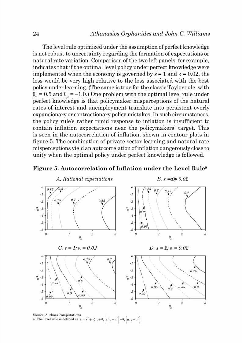
The level rule optimized under the assumption of perfect knowledge

is not robust to uncertainty regarding the formation of expectations or

natural rate variation. Comparison of the two left panels, for example,indicates that if the optimal level policy under perfect knowledge wereimplemented when the economy is governed by s = 1 and κ = 0.02, the

loss would be very high relative to the loss associated with the bestpolicy under learning. (The same is true for the classic Taylor rule, withθ

π = 0.5 and θ

u = –1.0.) One problem with the optimal level rule under

perfect knowledge is that policymaker misperceptions of the naturalrates of interest and unemployment translate into persistent overly

expansionary or contractionary policy mistakes. In such circumstances,

the policy rule’s rather timid response to inflation is insufficient tocontain inflation expectations near the policymakers’ target. Thisis seen in the autocorrelation of inflation, shown in contour plots infigure 5. The combination of private sector learning and natural rate

misperceptions yield an autocorrelation of inflation dangerously close tounity when the optimal policy under perfect knowledge is followed.

Figure 5. Autocorrelation of Inflation under the Level Rulea


C. s = 1; κ = 0.02 D. s = 2; κ = 0.02




Level rules of this type entail a tradeoff between achieving optimal

performance in one model specification and being robust to model

misspecification. We have shown that the optimal rule under perfectknowledge is not robust to the presence of imperfect knowledge. For

our benchmark case with imperfect knowledge, s = 1 and κ = 0.02, a

rule with response coefficients close to θπ = 1.5 and θu = –1.5 would

be best in this family. The greater responsiveness to inflation in this

parameterization proves particularly helpful for improving economic

stability here, but this policy performs noticeably worse if knowledge

is, in fact, perfect.

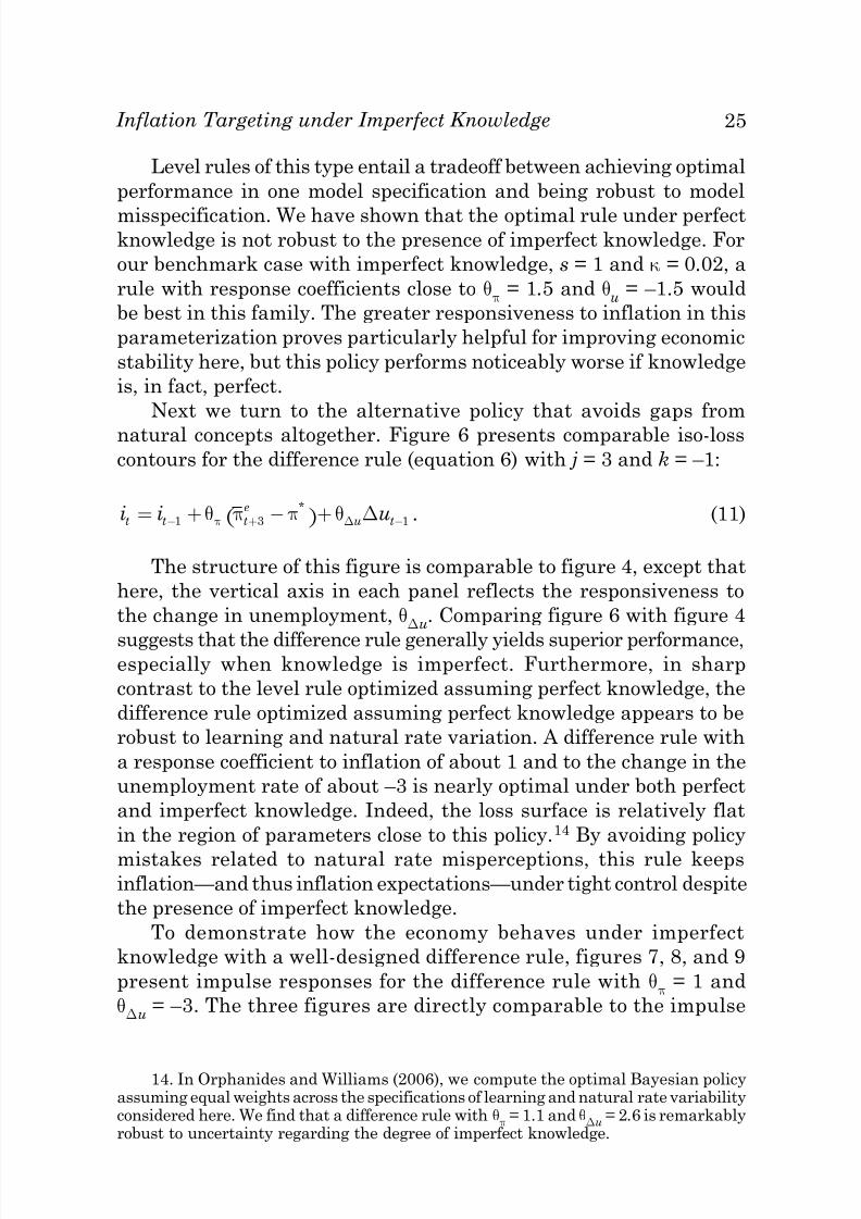
Next we turn to the alternative policy that avoids gaps from

natural concepts altogether. Figure 6 presents comparable iso-loss

contours for the difference rule (equation 6) with j = 3 and k = –1:

i i ut t te

u t= + −( )+− + −1 3 1θ π π θπ*

∆ ∆ . (11)

The structure of this figure is comparable to figure 4, except that

here, the vertical axis in each panel reflects the responsiveness to

the change in unemployment, θ∆u. Comparing figure 6 with figure 4

suggests that the difference rule generally yields superior performance,especially when knowledge is imperfect. Furthermore, in sharp

contrast to the level rule optimized assuming perfect knowledge, the

difference rule optimized assuming perfect knowledge appears to be

robust to learning and natural rate variation. A difference rule with

a response coefficient to inflation of about 1 and to the change in the

unemployment rate of about –3 is nearly optimal under both perfect

and imperfect knowledge. Indeed, the loss surface is relatively flat

in the region of parameters close to this policy.14 By avoiding policy

mistakes related to natural rate misperceptions, this rule keepsinflation—and thus inflation expectations—under tight control despite

the presence of imperfect knowledge.

To demonstrate how the economy behaves under imperfect

knowledge with a well-designed difference rule, figures 7, 8, and 9

present impulse responses for the difference rule with θπ = 1 and

θ∆u= –3. The three figures are directly comparable to the impulse

14. In Orphanides and Williams (2006), we compute the optimal Bayesian policyassuming equal weights across the specifications of learning and natural rate variability




responses for the Taylor rule shown earlier in figures 1, 2, and 3.

These responses exhibit some overshooting and secondary cycling,

as is typical of difference rules. The resulting loss, however, is

significantly lower than that resulting under the level rules that

may not exhibit such oscillations. In contrast to the impulseresponses under the Taylor rule, the 70 percent range of impulse

responses under the difference rule shown in these figures is much

tighter and concentrated around the impulse response under perfect

knowledge. This serves to demonstrate the relative usefulness of

this strategy for mitigating the role of imperfect knowledge in the

economy. In particular, figures 8 and 9 show that even without

incorporating explicit information about the policymakers’ objective

in the formation of expectations, this policy rule succeeds in

anchoring long-horizon expectations, especially of inflation, under

imperfect knowledge

Figure 6. Performance of the Difference Rulea

A. Rational expectations B. s = 0;κ

= 0.02

C. s = 1; κ = 0.02 D. s = 2; κ = 0.02


a. The difference rule is defined as i i ut t te

u t= + −

+− + −1 3 1θ π π θπ

*∆ ∆ .



Figure 7. Impulse Response Functions

under the Difference Rulea





a. The difference rule is defined as i i ut t t

e

t= + −

−− + −1 3 11 3π π* ∆ . The graphs display rational expectations with




Figure 8. Impulse Response to an Inflation Shock under the

Difference Rulea






e

t= + −












e

t= + −






4.2 Forecast Horizons

Throughout the analysis so far, we have assumed that the policyrule responds to expected inflation at a three-quarter-ahead horizonand to the lagged unemployment rate or the lagged change in theunemployment rate. We also explicitly examine the choice of horizonfor the class of difference rules. We find that under perfect knowledge,an outcome-based difference rule that responds to lagged inflation andunemployment performs about as well as forward-looking alternatives,consistent with the findings of Levin, Wieland, and Williams (2003).Under imperfect knowledge, however, an optimized difference rule

that responds to the three-quarter horizon for expected inflationoutperforms its outcome-based counterpart. As discussed in Orphanidesand Williams (2005a), under learning, inflation expectations representan important state variable for determining actual inflation that is notcollinear with lagged inflation. Expected inflation can thus be a moreuseful summary statistic for inflation in terms of a policy rule.15

The inflation forecast horizon in the policy rule should not betoo far in the future. Rules that respond to inflation expected two ormore years ahead generally perform very poorly. Such rules are prone

to generating indeterminacy, as discussed by Levin, Wieland, andWilliams (2003). In contrast to inflation, the optimal horizon for thechange in the unemployment rate is –1, meaning that policy shouldrespond to the most recent observed change in unemployment (thatis, for the previous quarter), as opposed to a forecast of the change inthe unemployment rate in subsequent periods.

4.3 Alternative Preferences

Next, we explore the sensitivity of the simple policy rules weadvocate as a benchmark for successful policy implementation tothe assumed underlying policymaker preferences. In our benchmarkparameterization, we examined preferences with a unit weight oninflation variability and a weight, λ = 4, on unemployment variability,noting that from Okun’s law this implies equal weights on inflationand output gap variability. As with various other aspects of thepolicy problem we examine, however, it is unrealistic to assume that

15. Using a simpler model, Orphanides and Williams (2005a) show that withcertain parameterizations of the loss function, it is best to respond to actual inflation,while in others, it pays to respond to expected inflation. A hybrid rule that responds to




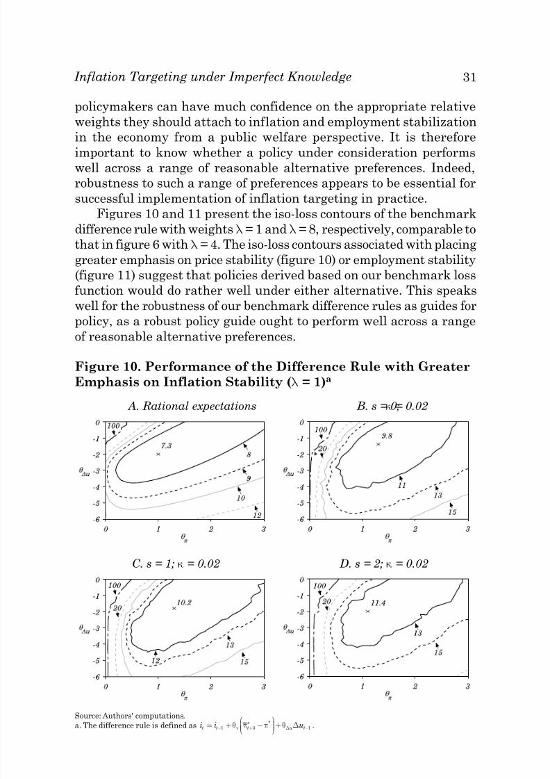
policymakers can have much confidence on the appropriate relative

weights they should attach to inflation and employment stabilization

in the economy from a public welfare perspective. It is thereforeimportant to know whether a policy under consideration performs

well across a range of reasonable alternative preferences. Indeed,

robustness to such a range of preferences appears to be essential for

successful implementation of inflation targeting in practice.

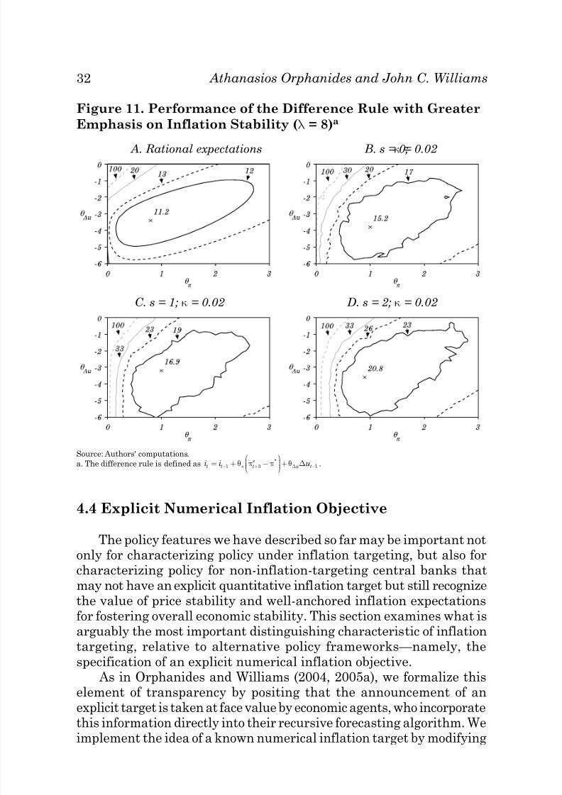
Figures 10 and 11 present the iso-loss contours of the benchmark

difference rule with weights λ = 1 and λ = 8, respectively, comparable to

that in figure 6 with λ = 4. The iso-loss contours associated with placing

greater emphasis on price stability (figure 10) or employment stability

(figure 11) suggest that policies derived based on our benchmark lossfunction would do rather well under either alternative. This speaks

well for the robustness of our benchmark difference rules as guides for

policy, as a robust policy guide ought to perform well across a range

of reasonable alternative preferences.

Figure 10. Performance of the Difference Rule with Greater

Emphasis on Inflation Stability (λ = 1)a


C. s = 1; κ = 0.02 D. s = 2; κ = 0.02




4.4 Explicit Numerical Inflation Objective

The policy features we have described so far may be important not

only for characterizing policy under inflation targeting, but also forcharacterizing policy for non-inflation-targeting central banks thatmay not have an explicit quantitative inflation target but still recognize

the value of price stability and well-anchored inflation expectationsfor fostering overall economic stability. This section examines what isarguably the most important distinguishing characteristic of inflationtargeting, relative to alternative policy frameworks—namely, the

specification of an explicit numerical inflation objective.

As in Orphanides and Williams (2004, 2005a), we formalize this

element of transparency by positing that the announcement of anexplicit target is taken at face value by economic agents, who incorporatethis information directly into their recursive forecasting algorithm We

Figure 11. Performance of the Difference Rule with Greater

Emphasis on Inflation Stability (λ = 8)a


C. s = 1; κ = 0.02 D. s = 2; κ = 0.02



e

u t= + −

+− + −1 3 1θ π π θπ

*∆ ∆ .




the learning model that agents use in forecasting to have the propertythat inflation asymptotically returns to target. No other changes are

made to the model or the learning algorithm. In essence, with a knowninflation target, agents need to estimate one fewer parameter in theirforecasting model for inflation than they would need to do if they didnot know the precise numerical value of the central bank’s inflationobjective. More precisely, we assume that agents estimate reduced-formforecasting equations for the unemployment rate and the inflation rate,

just as before. We then solve the resulting two-equation system for itssteady-state values of the unemployment rate and the interest rate,assuming that the steady-state inflation rate equals its target value.

We modify the forecasting equation for the interest rate by subtractingthe steady-state values of each variable from the observed values onboth sides of the equation and by eliminating the constant term. Thisequation is estimated using the constant-gain algorithm. The resultingthree-equation system has the property that inflation asymptoticallygoes to target. This system is used for forecasting as before.

To trace the role of a known target in the economy under alternativepolicy rules, we compute impulse responses corresponding to thesame policy rules examined earlier. Figure 12 shows the impulse

responses to the inflation and unemployment shocks for the classicparameterization of the Taylor rule, assuming that the central bankhas communicated its inflation objective to the public. Compared withfigure 1, the responses of inflation under imperfect knowledge are moretightly centered around the responses under perfect knowledge. Thedifferences are more noticeable when we examine long-run inflationexpectations. Figures 13 and 14 show the impulse responses of longer-run inflation and interest rate expectations, following the format of figures 2 and 3. The communication of an explicit numerical inflation

objective yields a much tighter range of responses of longer-runinflation expectations, centered around the actual target. Absent here isthe upward bias in the response of inflation expectations evident whenagents do not know the target. Interestingly, although knowledge of thelong-term inflation objective anchors long-term inflation expectationsmuch better, it is unclear whether this translates to a much reducedsensitivity of forward interest rates to economic shocks.16

16. These comparisons, however, are based on the assumption that forecasts of

these rates are governed by the same learning process governing the expectations forinflation and economic activity at shorter-horizons that matter for the determination of economic outcomes in the model. If, instead, the long-horizon interest rate expectations



Figure 12. Impulse Response Functions with Known π*







te

t t= + + −

− −

+ + −

* * *





Figure 13. Impulse Response to an Inflation Shock with

Known π* under the Taylor Rulea





a. The Taylor rule is defined as i r u ut t t

e

t

e

t t= + + −

− −

+ + −

* * *






with Known π* under the Taylor Rulea





a. The Taylor rule is defined as i r u ut t t

e

t

e

t t= + + −

− −

+ + −

* * *






Figures 15, 16, and 17 show the impulse responses corresponding

to the difference rule specified as above and assuming the central

bank has successfully communicated its objective to the public asdescribed above. Short-run expectations tend to cluster around

those that obtain under perfect knowledge. The median responses

are remarkably close to those under rational expectations, and the

70 percent ranges tend to be quite narrow, especially for inflation.

Long-horizon inflation expectations are extremely stable under the

difference rule coupled with an explicit numerical inflation objective.

For instance, the behavior of ten-year-ahead inflation expectations

is virtually indistinguishable from what would be expected under

perfect knowledge. Forward interest rates, however, continue to show

some small movements.

These impulse responses suggest that the expected benefits

of announcing an explicit inflation target may be quite different

depending on the policy rule in place. In terms of anchoring

long-horizon inflation expectations, for example, the benefits of a

known target seem considerably larger if policy follows the classic

parameterization of the Taylor rule than if policy is based on a well-

designed difference rule. The extent of these benefits also depends

on the precise degree of imperfections in the economy (that is, the

learning rate, κ, and variation in natural rates, s, in our model).

In the limiting case of rational expectations, for instance, the

“announcement” of the policymakers’ target in our model does

not make any difference at all, since agents already know the

policymakers’ preferences and objectives, by assumption.

To provide a clearer picture of the stabilization benefits of a

known inflation target in an environment of imperfect knowledge,

we compare the performance of an economy with a known targetto that with an unknown target for a given set of policies. Table 2

presents this comparison when expectations are formed with our

benchmark learning rate, κ = 0.02. In the top panel, we present the

results for the classic Taylor rule with θπ = 0.5 and θu

= –1.0, whose

properties under learning without a known inflation target were

examined in detail in section 3. In the middle panel, we present the

results for the Taylor rule with θπ = 1.5 and θu

= –1.5, which performs

best within this family of level rules when κ= 0.02 and s = 1. In the

bottom panel, we present comparable results for the difference rulewith θπ = 1 and θ∆u

= –3, which performs well even under learning



Figure 15. Impulse Response Functions with Known π*






a. The Taylor rule is defined as i i ut t t

e

t= + −

−− + −1 3 11 3π π* ∆ . The graphs display rational expectations with perfect

knowledge (RE), and median and 70 percent range of outcomes under learning with s = 1 and κ = 0.02



Figure 16. Impulse Response to an Inflation Shock with

Known π* under the Difference Rulea





a. The Taylor rule is defined as i i ut t te

t= + −

−− + −1 3 11 3π π* ∆ . The graphs display rational expectations with perfect





with Known π* under the Difference Rulea





a. The Taylor rule is defined as i i ut t tt

e= +

−− −+

−1 11 33

π π* ∆ . The graphs display rational expectations with perfect




b l e 2 .

T h e R o l e o f a n E x p l i c i t Q u a n t i t a t i v e I n f l a t i o n O b j e c t i v e a

U n k n o w n π *

K n o w n π *

s

S t a n d a r d d e v i a t i o n

S t a n d a r d d e v

i a t i o n

π

u – u *

∆ i

L o s s

A R ( π )

π

u – u *

∆ i

L o s s

A R ( π )

A .

T a y l o r r u l e

( θ

π =

0 .

5 ; θ

u =

– 1 .

0 )

0

3 . 6

6

0 . 9

9

2

. 8 0

2 5 . 1

0 . 8

6

3 .

3 7

0 .

9 5

2 .

6 7

2 2 . 1

0

. 8 4

1

4 . 3

5

1 . 1

1

3

. 0 1

3 2 . 9

0 . 9

0

3 .

7 6

1 .

0 4

2 .

8 0

2 6 . 4

0

. 8 7

2

5 . 2

1

1 . 2

4

3

. 2 9

4 4 . 2

0 . 9

3

4 .

2 1

1 .

1 8

3 .

0 2

3 2 . 5

0

. 9 0

B .

T a y l o r r u l e

( θ

π =

1 .

5 ; θ

u =

– 1 .

5 )

0

2 . 4

3

0 . 8

4

3

. 1 5

1 8 . 6

0 . 7

5

2 .

3 4

0 .

8 2

3 .

0 2

1 7 . 2

0

. 7 2

1

2 . 6

2

0 . 9

6

3

. 3 1

2 1 . 5

0 . 7

8

2 .

3 7

0 .

8 9

3 .

0 5

1 8 . 1

0

. 7 4

2

2 . 9

3

1 . 1

3

3

. 5 8

2 6 . 5

0 . 8

2

2 .

6 5

1 .

0 8

3 .

2 9

2 2 . 5

0

. 7 9

C .

D i f f e r e n c e

r u l e

( θ π

=

1 . 0 ; θ ∆ u

=

– 3 . 0

)

0

2 . 1

5

0 . 8

9

2

. 2 0

1 2 . 6

0 . 6

7

2 .

0 3

0 .

8 0

2 .

0 8

1 1 . 0

0

. 6 4

1

2 . 2

0

0 . 9

8

2

. 2 6

1 3 . 7

0 . 6

8

2 .

0 8

0 .

9 0

2 .

1 1

1 2 . 0

0

. 6 5

2

2 . 3

5

1 . 1

8

2

. 3 6

1 6 . 6

0 . 7

2

2 .

2 6

1 .

1 3

2 .

2 3

1 5 . 2

0

. 7 0

r c e : A u t h o r s ' c o m p u t a t i o n s .

l l e v a l u

a t i o n s a r e f o r t h e c a s e o f l e a r n i n g w

i t h κ

= 0 . 0

2 .

T h e l o s s f u n c t i o n c o r r e

s p o n d s t o e q u a t i o n ( 9 ) w i t h λ

= 4 a n

d v = 1 .

A R ( π ) d e n o t e s t h e f i r s t - o r d e r s e r i a l

e l a t i o n o f i n f l a t i o n .




The economy’s stabilization performance uniformly improves

with a known inflation target under all three rules. Successful

communication of an inflation target results in a modest reduction inthe persistence of inflation. In addition, for each rule, the variability of

inflation, real activity, and interest rates is smaller when the central

bank successfully communicates its numerical inflation objective

to the public. The extent of this improvement varies considerably,

however. The gains of making the target known appear substantial

under the classic Taylor rule. A more modest reduction in volatility is

evident for the more aggressive level rule, while the gains associated

with a known target are quite small when policy is based on the more

robust difference rule. These results suggest that the improvementassociated with successfully communicating a target can be rather

small, compared with the improvement that could be expected

from adopting the other elements of robust policies. For example,

abandoning policy based on even the best parameterization of the

level Taylor rule in favor of the robust difference rule yields a larger

benefit than communicating a numerical inflation objective while

continuing to follow a level rule.

5. CONCLUSION

Inflation targeting has been a very popular strategy among

central banks, particularly in small open economies. Researchers

have struggled, however, to pin down exactly what inflation targeting

means in terms of an implementable policy rule. To some, the Taylor

rule, or any monetary policy rule with a fixed long-run inflation

target, is a form of inflation targeting; to others, inflation targeting

is identified with solving a central bank optimization problem in a

rational expectations model. One shortcoming of these approaches

is that they abstract from the very cause that gave rise to inflation

targeting in the first place: the loss of a nominal anchor that transpired

under previous policy regimes in many countries.

This paper has attempted to put inflation-targeting strategy back

into the context in which it was born— namely, one in which inflation

expectations can endogenously drift away from the central bank’s goal.

We assume that private agents and the central bank have imperfect

knowledge of the economy; in particular, private agents attempt toinfer the central bank’s goals and reactions through past actions.

In such an environment key characteristics of inflation targeting in




close attention to inflation expectations—can influence the evolution

of inflation expectations and the economy’s behavior.

The problem of imperfect knowledge may be especially acutein small open economies and transition economies that have been

drawn to inflation targeting. Many of these countries have undergone

dramatic structural change over the past few decades. Consequently,

conclusions regarding the characteristics of optimal monetary policy

rules that are based on rational expectations models with perfect

knowledge cannot provide trustworthy guidance. Our analysis

suggests that policies formulated and communicated in terms of gaps

from natural rate concepts that are fundamentally unknowable may

be particularly problematic. A more reliable approach to successfullyimplementing inflation targeting is to search for monetary policy

strategies that are robust to imperfect knowledge.




REFERENCES

Batini, N. and A. Haldane. 1999. “Forward-Looking Rules for MonetaryPolicy.” In Monetary Policy Rules, edited by J.B. Taylor. University

of Chicago Press.

Beechey, M. 2004. “Learning and the Term Structure of Interest Ra-

tes.” University of California at Berkeley. Mimeographed.

Bernanke, B.S., Thomas Laubach, Frederic S. Mishkin, and Adam

Posen. 1999. Inflation Targeting: Lessons from the International

Experience. Princeton University Press.

Bernanke, B.S. and F.S. Mishkin. 1997. “Inflation Targeting: A New

Framework for Monetary Policy?” Journal of Economic Perspec-

tives 11(2): 97–116.

Clarida, R., J. Galí, and M. Gertler. 1999. “The Science of Monetary

Policy.” Journal of Economic Literature 37(4): 1661–707.

Clark, T. and S. Kozicki. 2005. “Estimating Equilibrium Interest

Rates in Real Time.” North American Journal of Economics and

Finance 16(3): 395–413.

Cogley, T. 2005. “Changing Beliefs and the Term Structure of Inter-

est Rates: Cross-Equation Restrictions with Drifting Parameters.”Review of Economic Dynamics 8(2): 420–51.

Cook, T. and T. Hahn. 1989. “The Effect of Changes in the Federal

Funds Rate Target on Market Interest Rates in the 1970s.” Journal

of Monetary Economics 24: 331–51.

Cukierman, A. and F. Lippi. 2005. “Endogenous Monetary Policy with

Unobserved Potential Output.” Journal of Economic Dynamics

and Control 29(11): 1951–83.

Croushore, D. 1993. “Introducing: The Survey of Professional Fore-

casters.” Federal Reserve Bank of Philadelphia Business Review (November): 3–13.

Croushore, D. and T. Stark. 2001. “A Real-Time Data Set for Macroeco-

nomists.” Journal of Econometrics 105 (November), 111–30.

Evans, G. and S. Honkapohja. 2001. Learning and Expectations in

Macroeconomics. Princeton University Press.

Faust, J. and D.W. Henderson. 2004. “Is Inflation Targeting Best-

Practice Monetary Policy?” Federal Reserve Bank of St. Louis

Review 86(4): 117–44.

Fuhrer, J.C. and G.R. Moore. 1995a. “Forward-Looking Behavior andthe Stability of a Conventional Monetary Policy Rule.” Journal of




. 1995b. “Inflation Persistence.” Quarterly Journal of Econo-

mics 110(1): 127–59.

Gaspar, V. and F. Smets. 2002. “Monetary Policy, Price Stability, andOutput Gap Stabilisation.” International Finance 5(2): 193–211.

Gaspar, V., F. Smets, and D. Vestin. 2005. “Optimal Monetary Policy

under Adaptive Learning. ” Working paper. Frankfurt: European

Central Bank.

Goodfriend, M. 1993. “Interest Rate Policy and the Inflation Scare

Problem: 1979–1992.” Federal Reserve Bank of Richmond Econo-

mic Quarterly 79(1): 1–23.

. 2004. “Inflation Targeting in the United States?” In The In-

flation Targeting Debate , edited by B. Bernanke and M. Woodford.

University of Chicago Press.

Goodfriend, M., and R. King. 1997. “The New Neoclassical Synthesis

and the Role of Monetary Policy.” In NBER Macroeconomics An-

nual 1997, edited by B.S. Bernanke and J. Rotemberg, 231–83.

MIT Press.

Gürkaynak, R., B. Sack, and E. Swanson. 2005. “The Sensitivity of

Long-Term Interest Rates to Economic News: Evidence and Im-

plication for Macroeconomic Models.” American Economic Review

95(1): 425–36.

Judd, J.P. and B. Motley. 1992. “Controlling Inflation with an Interest

Rate Instrument.” Federal Reserve Bank of San Francisco Econo-

mic Review 3: 3–22.

Kozicki, S. and P.A. Tinsley. 2001a. “Term Structure Views of Mo-

netary Policy under Alternative Models of Agent Expectations.”

Journal of Economic Dynamics and Control 25(1–2): 149–84.

. 2001b. “What Do You Expect? Imperfect Policy Credibility

and Tests of the Expectations Hypothesis.” Working paper 01-02.Federal Reserve Bank of Kansas City.

Kuttner, K.N. 2001. “Monetary Policy Surprises and Interest Rates:

Evidence from the Fed Funds Futures Market.” Journal of Mone-

tary Economics 47(3): 523–44.

Laubach, T. and J.C. Williams. 2003. “Measuring the Natural Rate of

Interest.” Review of Economics and Statistics 85(4): 1063–70.

Leiderman, L. and L.E.O. Svensson, eds. 1995. Inflation Targets.

London: Centre for Economic Policy Research.

Levin, A., V. Wieland, and J. Williams. 1999. “Robustness of SimpleMonetary Policy Rules under Model Uncertainty.” In Monetary




. 2003. “The Performance of Forecast-Based Policy Rules

under Model Uncertainty.” American Economic Review 93(3):

622–45.Mankiw, N.G. and L.H. Summers. 1984. “Do Long-Term Interest Rates

Overreact to Short-Term Interest Rates?” Brookings Papers on

Economic Activity 1984(1): 223–42.

McCallum, B.T. 1988. “Robustness Properties of a Rule for Monetary

Policy.” Carnegie-Rochester Conference Series on Public Policy 29:

173–203.

McCallum, B.T. and E. Nelson. 1999. “Performance of Operational

Policy Rules in an Estimated Semi-Classical Structural Model.”

In Monetary Policy Rules, edited by J.B. Taylor. University of Chicago Press.

Milani, F. 2005. “Expectations, Learning, and Macroeconomic Persis-

tence.” Univeristy of California at Irvine. Mimeographed.

Okun, A. 1962. “Potential Output: Its Measurement and Significan-

ce.” In American Statistical Association 1962 Proceedings of the

Business and Economic Section. Washington: American Statistical

Association.

Orphanides, A. 2003a. “Historical Monetary Policy Analysis and the

Taylor Rule.” Journal of Monetary Economics 50(5): 983–1022.. 2003b. “Monetary Policy Evaluation with Noisy Informa-

tion.” Journal of Monetary Economics 50(3): 605–31.

Orphanides, A. and S. van Norden. 2002. “The Unreliability of Output

Gap Estimates in Real Time.” Review of Economics and Statistics

84(4): 569–83.

Orphanides, A. and J.C. Williams. 2002. “Robust Monetary Policy Ru-

les with Unknown Natural Rates.” Brookings Papers on Economic

Activity 2002(2): 63–118.

. 2004. “Imperfect Knowledge, Inflation Expectations, and

Monetary Policy.” In The Inflation Targeting Debate, edited by

B.S. Bernanke and M. Woodford. University of Chicago Press.

. 2005a. “Inflation Scares and Forecast-Based Monetary Po-

licy.” Review of Economic Dynamics 8(2): 498–527.

. 2005b. “Robust Monetary Policy with Imperfect Knowledge.”

Federal Reserve Bank of San Francisco. Mimeographed.

. 2005c. “The Decline of Activist Stabilization Policy: Natu-

ral Rate Misperceptions, Learning, and Expectations.” Journal of

Economic Dynamics and Control 29(11): 1927–50.

2006 “Monetary Policy with Imperfect Knowledge ” Journal




Roberts, J.M. 1997. “Is Inflation Sticky?” Journal of Monetary Eco-

nomics 39(2): 173–96.

Roley, V.V. and G.H. Sellon. 1995. “Monetary Policy Actions andLong-Term Interest Rates.” Federal Reserve Bank of Kansas City

Economic Quarterly 80(4): 77–89.

Rotemberg, J.J. and M. Woodford. 1999. “Interest Rate Rules in an

Estimated Sticky Price Model.” In Monetary Policy Rules, edited

by J.B. Taylor. University of Chicago Press.

Rudebusch, G. 2002. “Assessing Nominal Income Rules for Moneta-

ry Policy with Model and Data Uncertainty.” Economic Journal

112(479): 402–32.

Sargent, T.J. 1993. Bounded Rationality in Macroeconomics. OxfordUniversity Press.

. 1999. The Conquest of American Inflation. Princeton Uni-

versity Press.

Sheridan, N. 2003. “Forming Inflation Expectations.” Johns Hopkins

University. Mimeographed.

Shiller, R.J. 1979. “The Volatility of Long-Term Interest Rates and

Expectations Models of the Term Structure.” Journal of Political

Economy 87(6): 1190–219.

Smets, F. 2003. “Maintaining Price Stability: How Long Is the MediumTerm?” Journal of Monetary Economics 50(6): 1293–309.

Taylor, J.B. 1993. “Discretion versus Policy Rules in Practice.” Carne-

gie-Rochester Conference Series on Public Policy 39: 195–214.

Wicksell, K. 1936 [orig. ed. 1898]. Interest and Prices. Translated by

R. F. Kahn. London: Macmillan.

Williams, J.C. 2005. “Robust Estimation and Monetary Policy with

Unobserved Structural Change.” In Models and Monetary Policy:

Research in the Tradition of Dale Henderson, Richard Porter,

and Peter Tinsley, edited by J. Faust, A. Orphanides, and D.L.

Reifschneider. Washington: Board of Governors of the Federal

Reserve System.

Woodford, M. 2003. Interest and Prices: Foundations of a Theory of

Monetary Policy. Princeton University Press.

Zarnowitz, V. and P.A. Braun. 1993. “Twenty-Two Years of the

NBER-ASA Quarterly Economic Outlook Surveys: Aspects and

Comparisons of Forecasting Performance.” In Business Cycles, In-

dicators, and Forecasting , edited by J.H. Stock and M.W. Watson.

University of Chicago Press.



Documentos de Trabajo

Banco Central de Chile

Working Papers

Central Bank of Chile

NÚMEROS ANTERIORES PAST ISSUES

La serie de Documentos de Trabajo en versión PDF puede obtenerse gratis en la dirección electrónica:www.bcentral.cl/esp/estpub/estudios/dtbc. Existe la posibilidad de solicitar una copia impresa con uncosto de $500 si es dentro de Chile y US$12 si es para fuera de Chile. Las solicitudes se pueden hacer por fax:(56-2) 6702231 o a través de correo electrónico: [email protected].

Working Papers in PDF format can be downloaded free of charge from:www.bcentral.cl/eng/stdpub/studies/workingpaper. Printed versions can be ordered individually forUS$12 per copy (for orders inside Chile the charge is Ch$500.) Orders can be placed by fax: (56-2) 6702231 ore-mail: [email protected].

DTBC-397

A Prize Worth Having: The IMF and Price StabilityAnne Krueger

Diciembre 2006

DTBC-396

Monetary Policy under Inflation Targeting: An IntroductionFrederic S. Mishkin y Klaus Schmidt-Hebbel

Diciembre 2006

DTBC-395

The Backus-Smith Puzzle: The Role of ExpectationsLuis Opazo

Diciembre 2006

DTBC-394 Overshooting Meets Inflation TargetingJosé De Gregorio y Eric Parrado

Diciembre 2006

DTBC-393 The “Great Moderation” and the Monetary TransmissionMechanism in ChileCristina Betancour, José De Gregorio , y Juan Pablo Medina

Diciembre 2006

DTBC-392

Regularidades Empíricas del Entorno Internacional de laEconomía ChilenaCarlos García, Patricio Jaramillo, y Jorge Selaive

Diciembre 2006

DTBC-391

Convergence and Long Run UncertaintyPablo Pincheira

Diciembre 2006



DTBC-390

The Quest for Price Stability in Central America and theDominican RepublicLuis Jácome y Eric Parrado

Diciembre 2006

DTBC-389 ¿Son Siempre las Universidades la Mejor Opción para un TítuloProfesional? Evidencia ChilenaPatricio Meller y David Rappoport

Diciembre 2006

DTBC-388

The Distribution of Assets, Debt and Income among ChileanHouseholdsPaulo Cox, Eric Parrado y Jaime Ruiz-Tagle

Diciembre 2006

DTBC-387

Financial Integration without the VolatilityRicardo Caballero y Kevin Cowan

Diciembre 2006

DTBC-386

La Información Contenida en los Movimientos de las Tasas Forward en ChileMauricio Larraín y Fernando Parro

Diciembre 2006

DTBC-385 Spreads Soberanos y Efecto ContagioÁlvaro García y Valentina Paredes

Diciembre 2006

DTBC-384

Actividad Especulativa y Precio del CobrePatricio Jaramillo y Jorge Selaive

Diciembre 2006

DTBC-383

Paths of Development, Specialization, and Natural ResourcesAbundanceRoberto Álvarez y Rodrigo Fuentes

Diciembre 2006

DTBC-382 Forecasting Canadian Time Series with the New-Keynesian Model

Ali Dib, Mohamed Gammoudi y Kevin Moran

Diciembre 2006

DTBC-381 An Estimated Stochastic General Equilibrium Model with Partial

Diciembre 2006

orphan ides & williams (2007)

Documents