orion entry flight control stability and performance (draft) · 2016-06-09 · orion entry flight...

Orion Entry Flight Control Stability and Performance (DRAFT)

Alan L Strahan1 NASA JSC, Houston, TX, 77058?

Greg R Loe2

Honeywell, Houston, TX, 77058

Pete Seiler3

Honeywell, Minneapolis, MN,55403

The Orion Spacecraft will be required to perform entry and landing functions for both Low Earth Orbit (LEO) and Lunar return missions, utilizing only the Command Module (CM) with its unique systems and GN&C design. This paper presents the current CM Flight Control System (FCS) design to support entry and landing, with a focus on analyses that have supported its development to date. The CM FCS will have to provide for spacecraft stability and control while following guidance or manual commands during exo-atmospheric flight, after Service Module separation, translational powered flight required of the CM, atmospheric flight supporting both direct entry and skip trajectories down to drogue chute deploy, and during roll attitude reorientation just prior to touchdown. Various studies and analyses have been performed or are on-going supporting an overall FCS design with reasonably sized Reaction Control System (RCS) jets, that minimizes fuel usage, that provides appropriate command following but with reasonable stability and control margin. Results from these efforts to date are included, with particular attention on design issues that have emerged, such as the struggle to accommodate sub-sonic pitch and yaw control without using excessively large jets that could have a detrimental impact on vehicle weight. Apollo, with a similar shape, struggled with this issue as well. Outstanding CM FCS related design and analysis issues, planned for future effort, are also briefly be discussed.

Nomenclature ANTARES = Advanced NASA Technology Architecture for Exploration Studies (simulation) CEV = Crew Exploration Vehicle CM = command module SM = service module FCS = flight control system RCS = reaction control system LEO = low earth orbit ISS = International Space Station PD = Proportional Derivative

I. Introduction HE CEV is envisioned by NASA to be a critical component of an overall Exploration architecture that ferries crews to and from the ISS after the shuttle retires in 2010, and eventually returns humans to the moon around

T

1 Insert Job Title, Department Name, Address/Mail Stop, and AIAA Member Grade for first author. 2 Insert Job Title, Department Name, Address/Mail Stop, and AIAA Member Grade for second author. 3 Insert Job Title, Department Name, Address/Mail Stop, and AIAA Member Grade for second author.

American Institute of Aeronautics and Astronautics

1

https://ntrs.nasa.gov/search.jsp?R=20070038284 2020-04-12T17:47:23+00:00Z

2020. The CEV mission will include returning to the earth from either of these scenarios, or possibly from an intermediate point due to an in-flight emergency. For all cases, the final phase of the return to earth will be Entry involving only the crew or cargo carrying Command Module (CM) portion of the CEV stack. The Entry phase will begin just after Service Module (SM) separation about 30 minutes prior to atmospheric entry interface (typically defined as 400,000 ft), and will extend through CM land or water landing. In general, Entry is also concerned with CM-only flight during aborts originating from ascent, however for brevity discussion of this category of Entry will not be included here.

The Entry FCS supports overall GN&C functionality by executing the attitude and rate commands that come out of guidance, while maintaining the stability of the CM. Stability is important to protect the crew and vehicle during entry, ensuring they are not exposed to excess rates due to vehicle tumbling. Closely following guidance commands is also critical to achieving a precision landing while staying within thermal and g-load boundaries that can be tolerated by the CM and crew. Once the parachutes are deployed during the final portion of the Entry phase, the Flight Control System is no longer utilized to maintain stability and control, except for executing the CM orientation maneuver prior to touchdown.

This paper covers significant results from a variety of analyses that have been accomplished to date, and that will better define the capabilities of the Entry FCS system. Preceding these analyses was the development and baseline of an Entry FCS design that is described briefly below. Once a baseline design was adopted, it was linearized along with aerodynamic and other CM vehicle characteristics, to support mathematical analysis of FCS stability and control authority, with an emphasis on the problematic subsonic flight regime. The baseline design was also incorporated into time domain simulations, where additional studies were performed covering topics including, fuel usage, minimum on and off pulse length and latency, maximum number of simultaneous jet required per string, and roll reorientation prior to touchdown. Furthermore, the dynamics and performance of a ballistic reentry of a slowly spinning CM, an emergency return option, were explored in time domain simulations. All of these aspects are important to the performance of the FCS and overall GN&C system, and its ability to deliver the crew and vehicle to a safe and survivable landing at the conclusion of a CEV flight.

II. Baseline FCS Design The CM Flight Control System design selected for baseline and analyzed throughout much of this paper was

originally developed by NASA-JSC to support early CEV Entry analysis started during the spring and summer of 2006. This design was adopted as part of an overall design philosophy to start simple and add complexity only as necessary to address identified limitations. The basic concept was a simple Proportional-Derivative (PD) design developed and tested in MATLAB and coded in the NASA ANTARES 6-degree of freedom high-fidelity simulation. The design multiplied gains by the attitude error (proportional path) and attitude rate error (derivative path), summed the products together and fed the result into a jet trigger logic. Trigger logic strategies included a simple Schmitt trigger with dead-band and hysteresis, or a more complicated phase plane trigger that considers both attitude and rate error directly. The resultant discrete jet command is then provided to jet selection logic to identify and fire the appropriate RCS jets, which are the only control effectors available to the CM.

Exo-atmospheric powered flight was an exception in that an alternate PD design with additional coordinate transformations to accommodate pointing commands in any direction and developed by CEV prime contractor Lockheed-Martin, was utilized for time domain analysis in the Lockheed-Martin SES 6-degree of freedom high fidelity simulation. For both of these designs, the first step in adding complexity to address performance limitations was simply to add gain schedules and tune these to achieve desired performance in support of CEV design cycles. The adjustments were based some on MATLAB analysis but primarily upon time domain Monte Carlo results with particular focus on aggressive bank command following during the first atmospheric pass of a lunar skip return trajectory.

Additional limitations with the baseline CM FCS design were identified as a result of the various analyses presented here, and will lead to further improvements in the overall design. These improvements will be explored as part of a new round of analyses during the summer and fall of 2007, and that will ultimately support the CEV Preliminary Design Review early in 2008. Fuel usage optimization is one area of particular interest that will be pursued, as to date FCS performance has primarily been focused on maintaining stability and supporting guidance in achieving precision targeting. Calculated lateral phase margins being less than the desired 30 deg during high speed atmospheric flight, due in part to estimated latency in the FCS loops, is another identified limitation. Gain optimization, adjustments to jet trigger logic and rate limiting, additional filters and coordinate transformations internal to the FCS are some areas that will be explored to address these limitations. If such modifications prove inadequate, than more sophisticated FCS design approaches like PID or LQR may be explored.


2

III. Linear Analysis

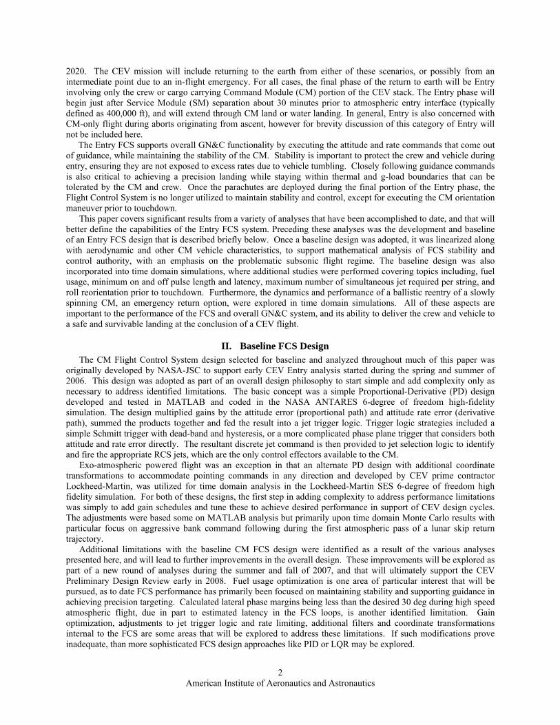
Passive Stability A root locus plot of the open loop pole locations is

shown in Figure 1. In the exo-atmospheric region the poles are grouped around the origin. As qbar increases two modes become oscillatory. One is the short period mode in the pitch axis and the other is the dutch roll mode in the lateral axis. Both modes have similar frequency and damping characteristics throughout most of the flight. The frequency of oscillations peaks as qbar peaks. For the ISS mission this happens at about Mach 6 and the oscillation frequency peaks at just above 3 rad/s. The vehicle is neutrally stable with the poles on or near the imaginary axis for most of the flight envelope. However, as the vehicle enters the transonic and subsonic regions both the short period and dutch roll modes become unstable.

Figure 1. Root locus of open loop poles during ISS mission.

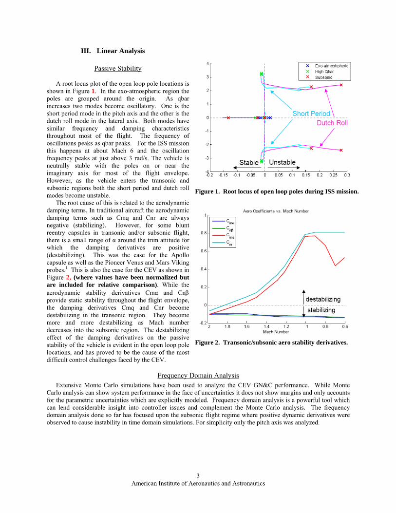
The root cause of this is related to the aerodynamic damping terms. In traditional aircraft the aerodynamic damping terms such as Cmq and Cnr are always negative (stabilizing). However, for some blunt reentry capsules in transonic and/or subsonic flight, there is a small range of α around the trim attitude for which the damping derivatives are positive (destabilizing). This was the case for the Apollo capsule as well as the Pioneer Venus and Mars Viking probes.1 This is also the case for the CEV as shown in Figure 2, (where values have been normalized but are included for relative comparison). While the aerodynamic stability derivatives Cmα and Cnβ provide static stability throughout the flight envelope, the damping derivatives Cmq and Cnr become destabilizing in the transonic region. They become more and more destabilizing as Mach number decreases into the subsonic region. The destabilizing effect of the damping derivatives on the passive stability of the vehicle is evident in the open loop pole locations, and has proved to be the cause of the most difficult control challenges faced by the CEV.

Figure 2. Transonic/subsonic aero stability derivatives.

Frequency Domain Analysis Extensive Monte Carlo simulations have been used to analyze the CEV GN&C performance. While Monte

Carlo analysis can show system performance in the face of uncertainties it does not show margins and only accounts for the parametric uncertainties which are explicitly modeled. Frequency domain analysis is a powerful tool which can lend considerable insight into controller issues and complement the Monte Carlo analysis. The frequency domain analysis done so far has focused upon the subsonic flight regime where positive dynamic derivatives were observed to cause instability in time domain simulations. For simplicity only the pitch axis was analyzed.


3

The RCS jets pose a particular challenge to linear analysis. The On-Off behavior of the jets is a “hard nonlinearity” which cannot be linearized. The describing function method was used to account for this non-linearity while predicting limit cycles, gain margins and phase margins.

Limit cycles can be stable or unstable. Unstable limit cycles are important because they represent the stability boundaries of the system.

The gain and phase margins obtained using describing functions have a slightly different interpretation than those for linear systems. A linear system is either stable or unstable. The gain and phase margins obtained using describing function analysis can be interpreted as the allowable changes in gain or phase before the system starts to limit cycle. In some cases however, limit cycle behavior may be unavoidable. In these cases the gain and phase margins can be interpreted as the allowable changes in gain or phase of the system before it stops limit cycling and becomes completely unstable.

An example of this type of analysis is shown in Figure 3. At Mach 0.6 the pitch axis has 2 unstable poles. These correspond to the short period mode. According to the Nyquist criteria a plot of the open loop transfer function must encircle the critical point twice in the counter-clockwise direction for the closed loop system to be stable. The critical point is traced by -1/N(A). Two limit cycles are predicted, one stable limit cycle with amplitude of 0.9 deg/sec in pitch rate, and one unstable limit cycle with amplitude of 15.7 deg/sec in pitch rate. Both limit cycles are at a frequency of 2.3 rad/sec. A nonlinear simulation shows verification of this in Figure 4. When the simulation was initialized with a pitch rate of 15 dps, the system converged to a stable limit cycle with an amplitude of around 1 deg/sec. When the simulation was initialized with a pitch rate of 16 deg/sec it diverged. Both of the responses are at the same frequency of about 2.3 rad/sec.

This type of analysis was repeated over the entire flight envelope. Figure 5 shows the predicted stability boundaries in terms of pitch rate in the transonic and subsonic regions from this analysis. It is evident that as Mach number decreases, the system’s ability to recover from perturbations to the trim state decreases dramatically. Gain and phase margins were also calculated. The pitch axis stability margins are very good as shown in Figure 6.

Null Controllability Regions It is reasonable to ask whether the stability

boundaries can be increased by a different controller or whether system redesign is required. This question cannot be answered using describing function

Figure 3. Mach 0.6 example describing function analysis.

Figure 4. Mach 0.6 simulation results.

Figure 5. Describing function predicted stability boundary.


4

analysis. To address this question, we consider the linear, short period approximation of the pitch axis dynamics. This system has two states, angle of attack and pitch rate (alpha and q) and is anti-stable in most of the transonic and subsonic regimes. Another significant aspect is that the system input, the torque due to the thrusters, is limited due to limited thruster forces. The placement of the thrusters is such that the thruster torque saturation is asymmetric, i.e. umin ≤ u ≤ umax where umin / umax are the min/max torques and umin ≠ umax.

The destabilizing pitch rate term in the short period model overpowers the limited thruster authority when the system is sufficiently far from the trim condition. Thus we anticipate that there are regions of the (alpha,q) phase plane for which no control law will be able to stabilize the short period mode. This idea is formalized by the concept of the Null Controllable Region (NCR) of an exponentially stable linear system with input saturation 1,2. The Null Controllability Region is the set of initial conditions for which there exists a control input to drive the system back to the trim condition. Hu, et. al. have given an explicit expression of the NCR boundary for a second order, unstable system.

Figure X1 shows the NCR in the (alpha,q) plane for Mach 0.5. The analysis by Hu, et. al. assumes that the saturation is symmetric. Thus we can use their results to plot the NCR under the assumption -umax ≤ u ≤ umax or umin ≤ u ≤ -umin. These are shown as the red and green curves in Figure X1, respectively. The CEV pitch thrusters have greater authority in the pitch up direction than the pitch down direction (|umin|≤ |umax|). As a result the NCR computed using umax is larger than the region computed for umin. The actual NCR computed based on the more realistic asymmetric thruster saturation, umin ≤ u ≤ umax, lies between these two curves. The NCR for the asymmetric thruster saturation can be computed by

solving a minimum time optimal control problem3. This requires a minor modification to the derivation in Bryson and Ho. The NCR for the assumption of asymmetric thruster saturation is shown as the blue curve in Figure 7. The minimum-time optimal control problem method is more computationally intensive than the explicit expression given by Hu, et.al. Thus all remaining results are computed using the expression by Hu, et.al. under the symmetric thruster assumption -umax ≤ u ≤ umax.

The size of the NCR indicates how robust any control law can be to wind gusts and other perturbations. No control law is able to stabilize the CEV once it is perturbed outside of this region. Thus a small NCR will mean difficultly controlling the vehicle. Figure 8 shows the NCR in the (delta-alpha, q) phase plane at various Mach numbers. Figure 9 shows the max delta-alpha and max q from the NCR regions versus

Figure 6. Describing function predicted stability margins for ISS mission.

-6 -4 -2 0 2 4 6

-10

-5

0

5

10

δα (deg)

q (d

eg/s

ec)

Symm. NCR for umaxAsymm. NCRSymm. NCR for umin

Figure 7 Null Controllability Regions for Mach 0.5

Figure 8. Null controllability region vs. Mach number.


5

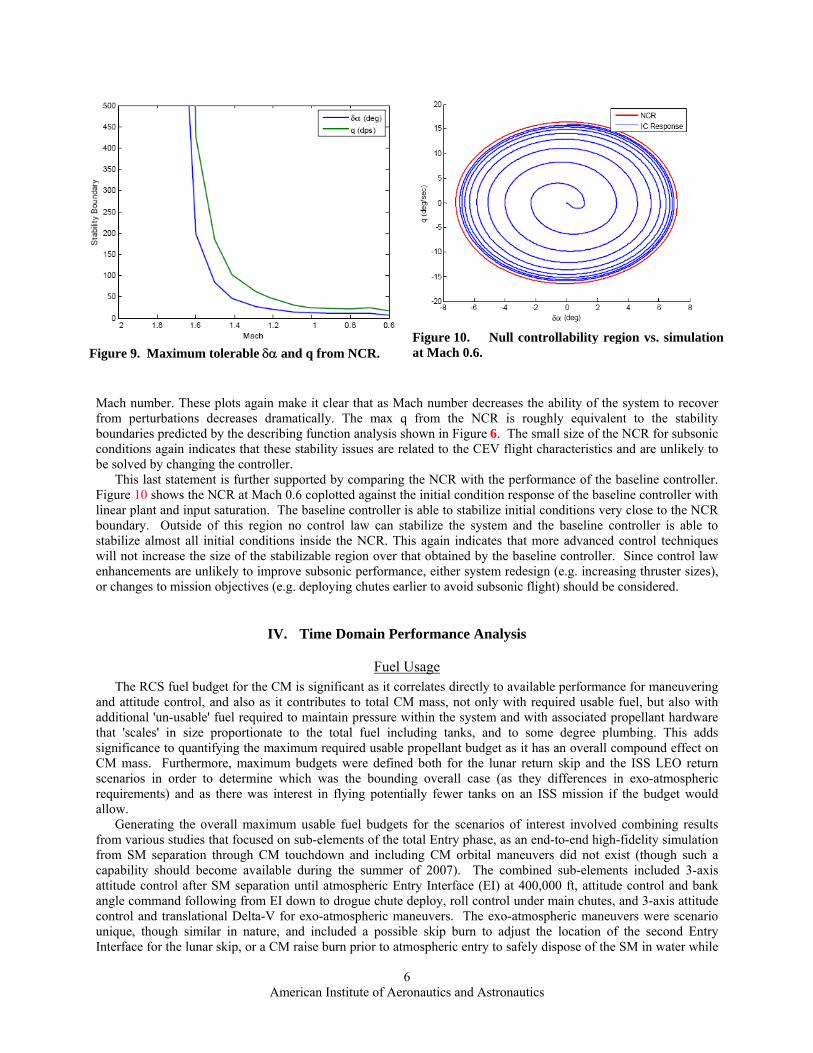
Mach number. These plots again make it clear that as Mach number decreases the ability of the system to recover from perturbations decreases dramatically. The max q from the NCR is roughly equivalent to the stability boundaries predicted by the describing function analysis shown in Figure 6. The small size of the NCR for subsonic conditions again indicates that these stability issues are related to the CEV flight characteristics and are unlikely to be solved by changing the controller.

This last statement is further supported by comparing the NCR with the performance of the baseline controller. Figure 10 shows the NCR at Mach 0.6 coplotted against the initial condition response of the baseline controller with linear plant and input saturation. The baseline controller is able to stabilize initial conditions very close to the NCR boundary. Outside of this region no control law can stabilize the system and the baseline controller is able to stabilize almost all initial conditions inside the NCR. This again indicates that more advanced control techniques will not increase the size of the stabilizable region over that obtained by the baseline controller. Since control law enhancements are unlikely to improve subsonic performance, either system redesign (e.g. increasing thruster sizes), or changes to mission objectives (e.g. deploying chutes earlier to avoid subsonic flight) should be considered.

IV. Time Domain Performance Analysis

Fuel Usage The RCS fuel budget for the CM is significant as it correlates directly to available performance for maneuvering

and attitude control, and also as it contributes to total CM mass, not only with required usable fuel, but also with additional 'un-usable' fuel required to maintain pressure within the system and with associated propellant hardware that 'scales' in size proportionate to the total fuel including tanks, and to some degree plumbing. This adds significance to quantifying the maximum required usable propellant budget as it has an overall compound effect on CM mass. Furthermore, maximum budgets were defined both for the lunar return skip and the ISS LEO return scenarios in order to determine which was the bounding overall case (as they differences in exo-atmospheric requirements) and as there was interest in flying potentially fewer tanks on an ISS mission if the budget would allow.

Figure 10. Null controllability region vs. simulation at Mach 0.6. Figure 9. Maximum tolerable δα and q from NCR.

Generating the overall maximum usable fuel budgets for the scenarios of interest involved combining results from various studies that focused on sub-elements of the total Entry phase, as an end-to-end high-fidelity simulation from SM separation through CM touchdown and including CM orbital maneuvers did not exist (though such a capability should become available during the summer of 2007). The combined sub-elements included 3-axis attitude control after SM separation until atmospheric Entry Interface (EI) at 400,000 ft, attitude control and bank angle command following from EI down to drogue chute deploy, roll control under main chutes, and 3-axis attitude control and translational Delta-V for exo-atmospheric maneuvers. The exo-atmospheric maneuvers were scenario unique, though similar in nature, and included a possible skip burn to adjust the location of the second Entry Interface for the lunar skip, or a CM raise burn prior to atmospheric entry to safely dispose of the SM in water while


6

increasing the capability of the CM to achieve targets further inland for the ISS mission. Additionally, the exo-atmospheric maneuvers each had two constituent budgets where one was for propellant required to provide the basic translational delta-v, thrusting through 2 opposing yaw jets minimizing yaw and off-axis torques, and a second was for propellant required to maintain direction during the burn and to maneuver to and from the burn attitude.

The lunar skip maximum usable propellant budget is provided in figure-11. The first row captures 'On-orbit' 3-axis attitude control from SM separation until Entry Interface, typically lasting about 30 minutes. The 30 lbm for this value was derived in part from a 6-DOF coasting simulation and from engineering judgment observing high fuel usage due to rapid limit cycling related to command latency, and where the FCS had not been tuned with regards to fuel efficiency, again an objective of the new design cycle. The second row capturing 200 lbm fuel usage for 'Atmospheric flight' was the worst fuel usage case from the 45000 Monte Carlo runs during the guidance merger activity between the NASA NSEG algorithm and the Draper PredGuid algorithm spanning 5 different lunar return scenarios from long range skip (~5300 nm) to lunar direct (~2000 nm) and three different landing sites for each using the ANTARES simulation. The next row, capturing 40 lbm for 'Roll control under main chutes' was derived from parametric analysis using a MATLAB simulation including CM inertias and RCS performance degraded for sea-level ambient pressure, and including a model of resistance torque from the main parachutes pulling outward on their riser lines, resisting twist that would result from a CM roll maneuver in this suspended configuration. The roll maneuver, intended to align the crew with the impact velocity, is assumed to never be more than 180 deg and to initiate at an altitude that would allow time for the maneuver, which current analysis shows to be optimally at 7 deg/sec. While the 40 lbm value has not yet been verified in a high-fidelity simulation, the methodology used in the MATLAB analysis is considered reasonable for this preliminary analysis. The fourth row, capturing 35 lbm for 'Skip Correction Burn Attitude Control' was derived from 6-DOF simulation by the Lockheed-Martin SES tool and accommodates a worst case of two full 180 degree pitch attitude maneuvers, one before the skip burn and one after, along with 90 degrees off axis excursions for thrust vector pointing during the powered flight translational maneuver. The attitude alignment maneuvers were limited only by 20 deg/sec each which was overly aggressive and will be tuned to be more fuel efficient. The values in the Delta-V column for these 4 entries are all derived from the propellant masses being the equivalent translational Delta-V that amount of propellant could deliver for a typical CM mass at entry. Finally the row for the 'Skip Correction Maneuver' captures 115 lbm and is the only row where the propellant mass is derived from a required delta-v, as 55 ft/s is the current desired value for a maximum skip correction burn. The magnitude of this value was defined based on engineering judgment as opposed to statistical results, as skip guidance algorithms currently satisfy targeting requirements without this Delta-V maneuver. Still there is a strong desire to protect it, or some significant portion of it, as the L/D of the evolving CM configuration is likely to drop below the 0.35 preferred value where analysis shows a very limited margin for guidance performance with several Monte Carlo cases saturating guidance for a significant amount of time (30+ seconds).

Delta-V (ft/s) Propellant (lbm) NotesAttitude ControlOn-orbit (post SM sep) 14 30 3-axis attitude control - approx 30 mins pre-EI to EIAtmospheric flight 96 200 Bank control, alpha/beta rate dampingRoll control under main chutes 19 40

Up to 180 deg maneuver under the main chutes to align vehicle with relative velocity

Skip Correction Burn Attitude Control 17 35

Up to two 180 degree pitch maneuvers and 90 degrees of thrust vector control

Translational Control

Skip Correction Maneuver 55 115Translational maneuver to adjust second entry point for drogue deploy target convergence

Sub-Total 129 270 Attitude control onlyTotal 201 420 Attitude control plus translational allocations Figure-11, Lunar Skip Return Maximum Propellant Budget

Compared to the previous analysis cycle maximum Lunar return fuel budget define in November 2006, most of these values have grown as the modeling fidelity and understanding of the Entry task has become more mature. Changes since the last cycle that have impacted the fuel budget include a ~10 to 15 % growth in rotational inertias, the addition of an 80 msec transport latency, extension of the applicable region for the unstable aerodynamic damping derivatives, a shift to using uniform dispersions for all aerodynamic uncertainties, updated altitude corrections on RCS thrust due to static pressure, and the increase in RCS thrust force dispersion to 15%. Also, as noted previously, the effort of this design cycle and the tuning of flight control design and gains has been focused on


7

landing accuracy performance and maintaining stability, with very little consideration to date on fuel budget. Exo-atmospheric attitude maneuvers and attitude hold are of particular interest for propellant usage improvement as these maneuvers are known to be sloppy, with frequent limit cycling due to latency and with overly aggressive attitude change maneuvers at 20 deg/sec that could perform slower with significant fuel savings.

The lSS return maximum usable propellant budget is provided in figure-12. As with the lunar skip case, the first row captures 'On-orbit' 3-axis attitude control for the roughly 30 minutes from SM separation until Entry Interface. The second row capturing 100 lbm fuel usage for 'Atmospheric flight' was the worst fuel usage case from a 3000 Monte Carlo study using the ANTARES simulation, and adding a modest additional fuel margin based on judgment that the test set was limited. The next row, capturing 40 lbm for 'Roll control under main chutes' was derived from the same MATLAB study as was used for the Lunar skip budget. The fourth row, capturing 20 lbm for 'CM Raise Burn Maneuver' was derived in a manner similar to that for the 'Skip correct Burn' except that smaller worst case maneuver angles were used, being a 90 deg pitch maneuver to and from burn attitude, along with 60 degrees off axis excursions for thrust vector pointing during the powered flight translational maneuver. The values in the Delta-V column for these 4 entries are all derived from the propellant masses being the equivalent translational Delta-V that amount of propellant could deliver for a typical CM mass at entry. Finally the row for the 'CM Raise Maneuver' captures 114 lbm and again is the only row where the propellant mass is derived from a required delta-v, as 55 ft/s is the current desired value for a maximum skip correction burn. The magnitude of this value was defined based on simulation analysis and engineering judgment, providing enough performance to target the SM for a water disposal while then extending the CM range sufficiently to reach Utah Test Range (the most inland of the initial landing site lists) for many of the ISS return scenarios and aggressive CM raise time-lines.

Delta-V (ft/s) Propellant (lbm) NotesAttitude ControlOn-orbit (post SM sep) 14 30 3-axis attitude control - approx 25 minsAtmospheric flight 48 100 Bank control, alpha/beta rate damping

Roll control under chutes 19 40Up to 180 deg maneuver under main chutes to align vehicle with relative velocity

CM Raise Burn Maneuver Attitude Control 10 20

Up to two 90 degree pitch maneuvers and 60 degrees of thrust vector control

Translational Control

CM Raise Maneuver 55 114Maneuver using yaw thrusters to increase the distance between the CM and SM/dock. Mech. disposal footprint

Sub-Total 82 170 Attitude control onlyTotal 146 304 Attitude control plus translational allocations Figure-12, ISS Return Maximum Propellant Budget

As with the lunar budget, when these results are compared to the previous analysis cycle maximum ISS fuel

budget defined in November 2006, some of these values have also grown as the modeling fidelity and understanding of the Entry task has become more mature. The same changes since the last design cycle listed above for the lunar budget, also are effecting this estimate, with the exception of the Atmospheric flight portion of the ISS budget which actually reduced by about 33 lbm since he November cycle. In November the atmospheric portion of the ISS budget was simply derived by starting with the lunar atmospheric budget, then subtracting an average amount of fuel used during the first atmospheric pass which was about 30 lbm. Again, the atmospheric portion of the ISS budget above is derived from simulation analysis with a modest reserve added. As with the lunar budget effort has begun towards optimizing fuel usage such that reductions are anticipated, whereas before the design goals focused only on targeting performance and stability.

Pulse Length and Latency Avionics and RCS propulsion hardware along with software design and execution methodology all affect the

overall performance of the CM Flight Control design, sometimes with significant impact, though to push back on such potentially limiting factors can adversely and overly constrain the complementary systems. In an effort to begin to address such concerns and understand how these spacecraft systems interact with the Flight Control a series of Monte Carlo studies were performed in a parametric manner as defined in the first 4 columns of Figure-13 below. It is intended that this study, along with any subsequent similar analysis, will provide the basis for defining Interface


8

Requirement Documents (IRD's) between the Entry GN&C Flight Control and other relevant systems, specifically Software, Avionics and CM RCS propulsion, which in turn capture agreed upon interface performance parameters

The interface or multiple-system spanning parameters that were studied here included Minimum allowable on and off pulse for a given RCS jet, overall end-to-end latency and flight control algorithm execution frequency. Performance metrics captured and compared for the various 1000 case Monte Carlo studies varying these input parameters included average and peak fuel usage, subsonic instability occurrence (per 1000 cases) and targeting performance, measured conversely as number of cases that missed the 2.7 nautical mile targeting radius at drogue chute deploy (also per 1000 cases). The targeting metric is not the same as what the overall Cm must ultimately achieve in that the 2.7 nautical mile radius defines the ground target including effects of wind drift under the chute, but as this is a separate on-going trade, the simpler criteria of applying targeting performance at drogue deploy was applied here and in a similar manner to all Monte Carlo studies. Subsonic instabilities were defined as any case that exceeded 40 deg from alpha = 180 or beta = 0 (heat shield forward) orientation.

Performance of a 'nominal' configuration was included as the last row of the table, where assumed minimum on and off RCS pulse durations were based on informal conversations with the RCS community early in 2007 and included a 60 milisec minimum on pulse accompanies by a 25 milisec minimum off pulse for a given RCS jet. This proved challenging to implement as the minimum off pulse was not a clean multiple of the on duration and neither were clean multiples of the 40 milisec minor cycle rate of operating the FCS at 25 Hz. To implement these odd pulse durations simulation logic was developed that individually tracked on and off times for each jet, and that adjusted the effective torque of that jet for every 40 milisec frame to reflect the amount of equivalent on time allowed for that minor cycle, assuming it was commanded on for that cycle. This would be functionally equivalent to the RCS hardware managing the on and off command timing of each jet in response to FCS jet commands and within the constraints of the minimum allowable on and off pulses. The calculation of the effective torque was also used for implementing the 60 on and 25 off case in the 50 Hz GNC block, whereas for all other Monte Carlo studies, with either 25 or 50 Hz GN&C rates, the simulation was adjusted to operate at 50 Hz for the equations of motion and jet command logic, allowing for a much cleaner implementation of the minimum on and off pulses being clean multiples of the 20 milisec minor cycle frame, and not requiring artificial torque adjustments. For all cases the GN&C software was operated at either the 25 or 50 Hz as noted (including navigation and Flight Control). Latency was added simply with a time based delay in the jet command logic, and as this was either 0 or 80, it was a clean multiple of either the 20 or 40 milisec minor cycle rate for all of the studies.

GNC Rate

Minimum on time

Minimum off time

RCS Lag

Ave fuel

Peak fuel

Subsonic

instabilities

Target misses

(Hz) (ms) (ms) (ms) (lbm) (lbm) (# cases) (# cases) 60 20 80 113.4 151.2 5 0 60 25 80 113.3 152.2 5 0 60 40 80 113.4 150.3 5 0 60 60 80 113.3 151.4 5 0 80 20 80 113.3 151.4 4 0 80 40 80 113.4 151.4 4 0 80 60 80 113.3 151.4 5 0 60 20 0 85.4 123.9 2 0

50Hz

80 20 0 88.4 122.7 3 0 60 40 80 133.6 180.0 4 0 25Hz 80 40 80 133.5 175.6 4 0

25Hz (nom) 60 25 80 133.0 173.3 4 0

Figure-13, FCS Performance Impacts from RCS Pulse Duration, Latency and Execution Frequency

One important observation these results show is that the torque varying assumptions used to implement the 60 milisec minimum on and 25 milisec minimum off pulse into a 40 milisec minor cycle simulation appears to be a reasonable approximation. This is bared out by comparison of the nominal 25 Hz 60/25/80 case (which uses the assumption) and the 60/40/80 case for 25 Hz FCS (which does not). For these, most metrics matched closely, with the peak fuel usage being slightly higher for the 40 milisec minimum off case. Similarly the 60/25/80 case in the 25


9

Hz GNC group matches even closer with the two 50Hz cases that bound it, the 60/20/80 and the 60/40/80 cases. This is important as most other FCS performance analysis of this design cycle and the skip guidance comparison activity also conducted during the spring of 2007 utilized this approximation. Other significant observations that can be drawn from the results of this table include: • Lag significantly increases fuel usage performance, where all other parameters are equal. This is evident by

comparing 80 ms lag cases to 0 ms lag cases (all in the 50 Hz GNC group), where fuel usage increases by 30 lbm while targeting performance changes little and subsonic instabilities change by 1 or 2 cases. • A higher calling frequency (50 Hz) for FCS can reduce fuel usage. This is evident by comparing 50 Hz cases to

25 Hz cases (with equivalent 80 milisec lags, etc), where fuel usage reduces by 20 lbm while targeting performance and subsonic instabilities change little if at all. • Increasing minimum on pulse to 80 milisec and increasing minimum off pulse to 40 or even 60 milisec, appears

to have little effect on overall GN&C performance. This is evident by comparing similar cases with comparable lags and GNC calling frequencies, where fuel usage, targeting and subsonic instabilities all show little comparative difference.

Maximum Jets per String The maximum number of RCS jets that can simultaneously be fired per string of jets has impacts both on RCS

system hardware design and on Flight Control performance. The baseline CM design for this analysis cycle had 3 independent strings of 6 jets each, where each of the 6 would provide torque primarily in a specific rotational direction (+/- Pitch, +/- Roll and +/- Yaw) though with some modest cross-coupling into other rotational axes. The baseline hardware redundancy requirements for the design cycle called for a fail-operational / fail-safe design, requiring mission success still be achievable with one string down and a survivable return be achievable with two strings down. This constrained nominal and emergency entry to operate with a single string of 6 RCS jets. The RCS community designed 3 complete strings of tanks, plumbing and other necessary hardware, only the sizing of plumbing, valves, etc for a given string was in part dependent on the total number of jets that could be fired simultaneously. As such, results from this study, and any subsequent related work, will also support the Interface Requirements Document (IRD) between the Entry GN&C Flight Control and the RCS hardware.

Performing exo-atmospheric translational maneuvers while also maintaining attitude control, was judged to be the most demanding of all Entry flight sub-phases in terms of requiring simultaneous jets. This was because exo-atmospheric coast was a simple 3-axis control and atmospheric flight involved bank command following along with alpha and beta damping, where none of these scenarios implied that opposing rotational jets would require simultaneous firing. However, powered translational flight, would nominally involve simultaneous firing of two opposing yaw jets to provide the Delta-V, while simultaneously providing for pitch and roll control, which in turn would imply the need for 4 simultaneous jets if the jets just listed were all active at once. While it would be straight forward in the flight software to simply allow for the commanding of 4 jets, limiting the commanding to 3 could allow for a smaller RCS system saving vehicle mass, if the performance with 3 wasn't overly degraded.

To explore this possibility a Monte Carlo study was performed where a 1000 case run set was generated allowing a maximum of 4 RCS jets during the execution of a lunar skip correction 'Kepler' translation maneuver. This was compared to another 1000 case run set where the number of simultaneously active jets was limited to 3, though with a prioritization logic incorporated to reduce the impact of having to delay one rotational axis until the other is finished. The prioritization strategy employed for this study was simple always reserving 2 jets for the yaw as they performed the translation maneuver, and though one yaw jet could 'off-pulse' to provide for yaw control, this was never made available to the other two rotational axis. Instead the other two axis had to share the one remaining active slot where prioritization was always given to the jet that was already active when the other was commanded, however if both the pitch and roll axes experienced a command at the same time, the axis with the larger attitude error would take priority.

Results from this study are provided in figure-14 below, which includes two tables. The first provides conditions at the second atmospheric Entry Interface after having completed the skip correction translation Delta-V during the preceding exo-atmospheric coast. The second table provides statistical results for fuel usage and Delta-V imparted from the Monte Carlo study, with both comparing results from the 1000 case run set limitng to 3 active jets vs the 1000 case set allowing 4 active jets. Comparing 2nd Entry Interface conditions shows virtually no discernable differences, where the Geodetic Latitude and Longitude matched for all displayed significant digits and with the Mean Geodetic Altitude differing by only about 15 ft, a trivially small difference. Comparing propellant and related jet firing data showed a little more discernable difference in the statistical results, but still very small and generally insignificant. The mean number of 4 jet firings being 3.28 for the 4 jet option is simply that the latter option would


10

fire 4 simultaneous jets for less then 4 minor cycle frames or less than 160 milisec of a 70+ second average maneuver duration. The most extreme case utilized 4 simultaneous jets for 97 minor cycles or 3.88 second of a 70+ second average maneuver. Mean and maximum translational Delta-V's along with lbm of propellant use for the translation are listed for both run sets in the middle row of the second table. In the bottom row, total mean and maximum propellant values are listed which includes propellant to perform attitude maneuvers to and from the burn attitude and propellant to provide control during the translational maneuver. The maneuver logic also occasionally performed unnecessary bank reversals that were not included in the adjusted maximum budget.

Jets / String 3 4Mean Geodetic Latitude (deg) 26.29 26.29

Std Dev. (deg) 1.09 1.09Mean Geodetic Longitude (deg) -112.87 -112.87

Std Dev. (deg) 0.29 0.29Mean Inertial Velocity (fps) 24905.98 24905.99

Std Dev. (fps) 86.6 86.55Mean Inertial Fligh Path Angle (deg) -1.59 -1.59

Std Dev. (deg) 0.31 0.31Mean Geodetic Altitude (ft) 272259.34 272274.21

Std Dev. (ft) 1509.39 1501.69

2nd Entry Initial Conditions

Jets / String 3 4Mean Number of 40 ms 4 jet firings 0 3.28

Maximum Number of 40 ms 4 jet firings (time) 0 97 (3.88)Mean Kepler DV fps (lbm) 32.9 (69.3) 32.9 (69.3)

Max limited to 55 fps (115 lbm) 55 (115) 55 (115)Mean Kepler DV Total Prop (lbm) 99.65 99.72

Adjusted Maximum (lbm) * 152 148

Skip Correction Propellant Usage

* Removes non-correction maneuver attitude control later during Kepler phase and 2 unnecessary 180 degree bank reversals Figure-14, Monte Carlo Results for Limiting to 3 vs 4 Active Jets During a Skip Correction Burn With a mean difference of about 0.07 lbm and a maximum difference of 4 lbm, and no appreciable difference in

targeting at the 2nd Entry Interface point, it was judged acceptable to limit the total number of simultaneously available jets per RCS string to 3, assuming some kind of jet prioritization logic would be used during the exo-atmospheric translational maneuvers.

Roll Reorientation for Touchdown Orion vehicle requirements currently exist that define the orientation of the CM and ultimately of the crew in

relation to the horizontal velocity of the vehicle at touchdown, should the velocity be faster than 10 ft/sec. This is primarily to orient impact loads in the most favorable direction for the crew, though also to minimize the potential for the CM to flip over at impact. As the CM capsule is hanging from the main parachutes attached to the CM apex at the time of impact, this effectively becomes a requirement to orient the CM Z-axis, using roll RCS jets, with regards to the horizontal velocity or heading.

To better understand this maneuver, a 6 degree of freedom MATLAB based time-domain simulation was developed to investigate fuel usage, altitude trigger range, turn rate and whether the roll RCS jets at sea level had sufficient torque to overpower the resistance torque from the twisting of the main parachute lines. The model included vehicle mass and RCS jet properties, reduced thrust for sea level ambient pressure, propellant flow rate, a simple phase plane controller and a parachute resistance torque model as a function of clock angle starting at zero


11

twist. The resistance torque model was estimate, with a maximum near 90 degrees twist that reduced again towards 180, and that will be measured in testing later this year. Some further assumptions included an additional -20% dispersion on the RSC thrust altitude correction (reducing RCS thrust more) and sink rates of approximately 28 ft/sec under 3 main chutes and 37 ft/sec under two, which was a scenario that had to be protected.

To identify the maximum resistance torque that the CM roll RCS could accommodate, a parametric analysis was performed as shown in figure-15. Simulations were performed where the entire twist resistance curve was scaled by percentages of the maximum predicted resistance twist profile, where a 90 deg reorientation was commanded and held. As would be expected, the roll RCS jet could maintain a 90 deg orientation and oppose a resistance twist torque equal to its altitude adjusted RCS torque, being 522 ft-lbs or about 65% of the worse case resistance profile. The roll RCS jet is unable to maintain orientation of 90 deg for resistance torques greater than 65% as these are observed to roll back to smaller twist values. As a 90 deg twist is near the peak predicted resistance torque, this is assumed to be the bounding case.

Figure-15, Roll Reorientation Performance holding 90 deg twist The ideal commanded roll rate for minimum fuel is demonstrated in figure-16 below. Plotted here are results

from time-based roll orientation simulations, again for varying chute twist resistance scaling factors across the bottom of the figure, with total fuel usage for a 180 deg maneuver listed along the left axis, and lines connecting the points of equal command heading rate. This shows that for the desired maximum resistance torque of 65 % (vertical dashed red line) that 7 and 14 deg/sec use the same fuel for a 180 deg maneuver, while the 2 deg/sec actually uses more. For lower twist resistance torques the 14 deg/sec uses the most fuel of the 3 turn rates. Overall, the 7 deg/sec commanded roll rate shows the best performance across the entire range of resistance torques.


12

Figure-16, Propellant usage vs Resistance Twist Torque for a given Roll Rate Figure-17, below shows the overall fuel usage and the workable altitude range for triggering a maximum 180

deg roll reorientation against a 65% scaled resistance torque profile, while staying within a 40 lbm budget. The lower altitude in the table, 1500 ft above ground level (AGL), is the minimum altitude for triggering the maneuver and turning 180 degrees against the 65 % scaled resistance torque while falling at the faster 37.5 ft/sec sink rate corresponding to a failed main chute, and using 17 lbm of fuel. The maximum trigger altitude is the case that most rapidly uses the currently budgeted 40 lbm of fuel, where the commanded roll reorientation is just 90 deg against a 65 % scaled resistance torque and where the RCS has to continuously fire to maintain the 90 deg orientation, and where the sink rate is the slower 28.6 ft/sec under 3 good chutes. This altitude to burn 40 lbm of fuel is just 2286 ft AGL, resulting in what may be a tight altitude range for triggering this maneuver depending on navigation performance.

AGL altitude (ft) Fuel usage (lbm) Roll change (deg) Time (sec)

Minimum Alt case 1500 17 180 40

Maximum Alt case 2286 40 90 80

Figure-17, Roll Reorientation Maneuver Bounding Cases Overall the reorientation maneuver appears feasible if the resistance torque is not too large (65 % the originally

predicted worse case) though fuel usage and navigation performance may yet become issues.

V. Emergency Ballistic Performance The provision of an Emergency Entry Mode has been called out in the Constellation Architecture and Orion

requirements where such a mode is generally defined as a minimal capability contingency type mode using dissimilar hardware and intended only to return the crew to a non-precision untargeted but survivable earth landing. This mode has mostly been envisioned to be a ballistic trajectory where primary capabilities to target or control the


13

vehicle have failed somewhere during the entry phase and the CM is spun up to minimize the effects of an arbitrary lift angle on the trajectory. This prevents a vehicle skip out (if the arbitrary bank angle was near lift up on a lunar return) and prevents excessive g-loads on the crew (if the arbitrary angle was near lift down), and brings the command module down rapidly, most likely to a water landing if on a lunar return. The Emergency Entry Mode concept presently just provides minimal alternative GN&C hardware and software capabilities to achieve the ballistic trajectory, either manually piloted or possibly a simple automated maneuver. A dissimilar method of activating the RCS jets is presently required for this mode as well, known as cold gas method, which simply vents the pressurized propellants out the RCS jets without ignition producing only a fraction of the normal vacuum thrust.

Active vs Passive Control In acknowledgment of the desire to keep the Emergency Entry Mode as simple as possible, the potential to

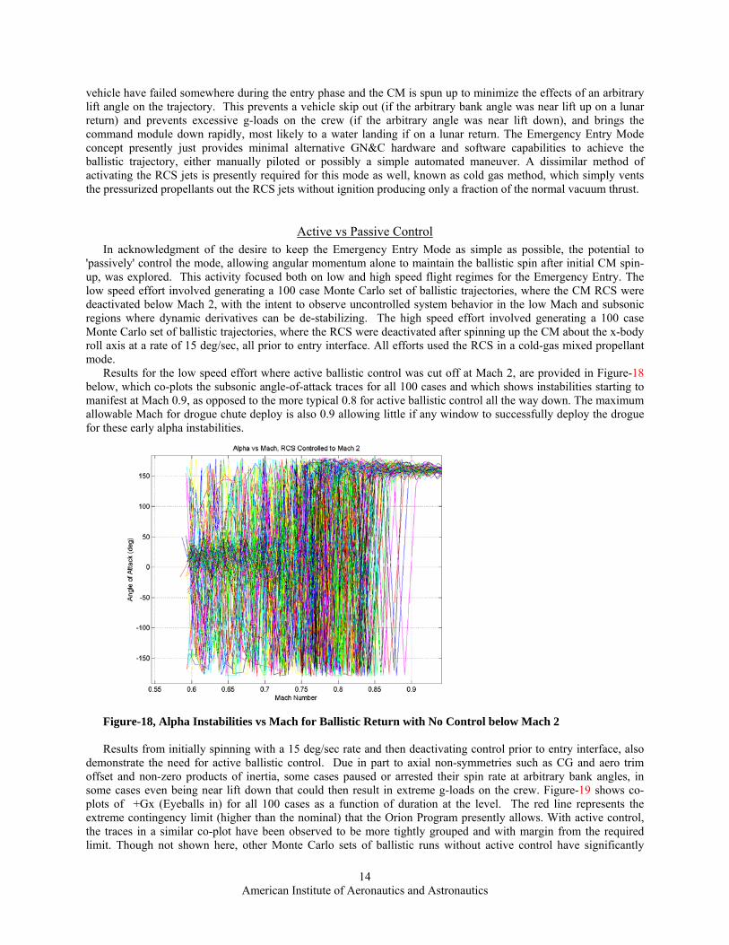
'passively' control the mode, allowing angular momentum alone to maintain the ballistic spin after initial CM spin-up, was explored. This activity focused both on low and high speed flight regimes for the Emergency Entry. The low speed effort involved generating a 100 case Monte Carlo set of ballistic trajectories, where the CM RCS were deactivated below Mach 2, with the intent to observe uncontrolled system behavior in the low Mach and subsonic regions where dynamic derivatives can be de-stabilizing. The high speed effort involved generating a 100 case Monte Carlo set of ballistic trajectories, where the RCS were deactivated after spinning up the CM about the x-body roll axis at a rate of 15 deg/sec, all prior to entry interface. All efforts used the RCS in a cold-gas mixed propellant mode.

Results for the low speed effort where active ballistic control was cut off at Mach 2, are provided in Figure-18 below, which co-plots the subsonic angle-of-attack traces for all 100 cases and which shows instabilities starting to manifest at Mach 0.9, as opposed to the more typical 0.8 for active ballistic control all the way down. The maximum allowable Mach for drogue chute deploy is also 0.9 allowing little if any window to successfully deploy the drogue for these early alpha instabilities.

Figure-18, Alpha Instabilities vs Mach for Ballistic Return with No Control below Mach 2 Results from initially spinning with a 15 deg/sec rate and then deactivating control prior to entry interface, also

demonstrate the need for active ballistic control. Due in part to axial non-symmetries such as CG and aero trim offset and non-zero products of inertia, some cases paused or arrested their spin rate at arbitrary bank angles, in some cases even being near lift down that could then result in extreme g-loads on the crew. Figure-19 shows co-plots of +Gx (Eyeballs in) for all 100 cases as a function of duration at the level. The red line represents the extreme contingency limit (higher than the nominal) that the Orion Program presently allows. With active control, the traces in a similar co-plot have been observed to be more tightly grouped and with margin from the required limit. Though not shown here, other Monte Carlo sets of ballistic runs without active control have significantly


14

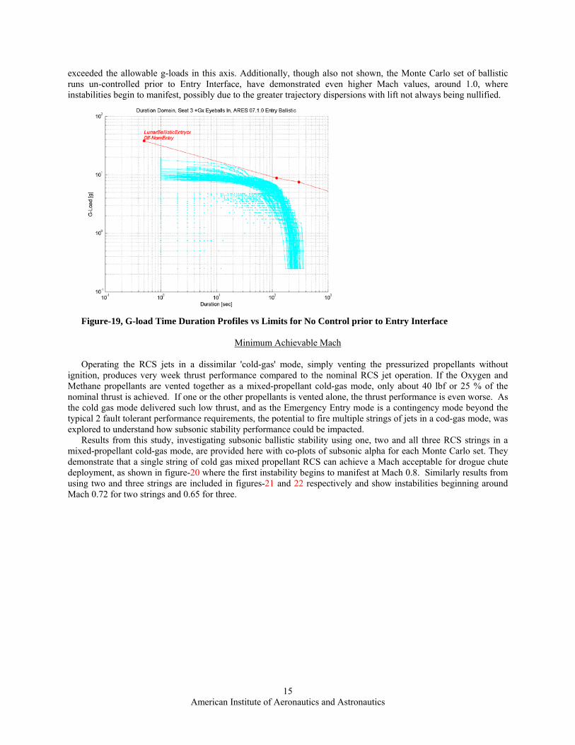
exceeded the allowable g-loads in this axis. Additionally, though also not shown, the Monte Carlo set of ballistic runs un-controlled prior to Entry Interface, have demonstrated even higher Mach values, around 1.0, where instabilities begin to manifest, possibly due to the greater trajectory dispersions with lift not always being nullified.

Figure-19, G-load Time Duration Profiles vs Limits for No Control prior to Entry Interface

Minimum Achievable Mach Operating the RCS jets in a dissimilar 'cold-gas' mode, simply venting the pressurized propellants without

ignition, produces very week thrust performance compared to the nominal RCS jet operation. If the Oxygen and Methane propellants are vented together as a mixed-propellant cold-gas mode, only about 40 lbf or 25 % of the nominal thrust is achieved. If one or the other propellants is vented alone, the thrust performance is even worse. As the cold gas mode delivered such low thrust, and as the Emergency Entry mode is a contingency mode beyond the typical 2 fault tolerant performance requirements, the potential to fire multiple strings of jets in a cod-gas mode, was explored to understand how subsonic stability performance could be impacted.

Results from this study, investigating subsonic ballistic stability using one, two and all three RCS strings in a mixed-propellant cold-gas mode, are provided here with co-plots of subsonic alpha for each Monte Carlo set. They demonstrate that a single string of cold gas mixed propellant RCS can achieve a Mach acceptable for drogue chute deployment, as shown in figure-20 where the first instability begins to manifest at Mach 0.8. Similarly results from using two and three strings are included in figures-21 and 22 respectively and show instabilities beginning around Mach 0.72 for two strings and 0.65 for three.


15

Figure-20, Alpha Instabilities vs Mach for 1-string Cold-Gas RCS

Figure-21, Alpha Instabilities vs Mach for 2-string Cold-Gas RCS

Figure-22, Alpha Instabilities vs Mach for 3-string Cold-Gas RCS These results demonstrate the sensitivity of Mach where instabilities begin occurring vs available thrust and

torque, where it is no surprise to observe that more torque allows for deeper penetration to lower Machs. Depending on the performance of a degraded navigation system in the EEMS mode, it may prove difficult to detect a drogue chute Mach trigger condition the protects against early deployment prior to Mach 0.9 that could damage the chute,


16

and a late deployment below Mach 0.8 where instabilities could occur. If this Mach range is insufficient, than the use of two strings of cold gas could be considered to open up the altitude range for EEMS chute trigger.

VI. Conclusion Overall results here demonstrate that the baseline CM Entry Flight Control System design can achieve the

primary design goals of following guidance commands and maintaining stability for all but a handful of subsonic conditions, though in a manner that at present exceeds the design fuel budget. Results also show that larger minimum on and off pulse sizes, being considered by the RCS community, so far have little impact on performance, though end-to-end latency has a significant impact on fuel usage while a faster FCS execution rate would provide a marginal improvement in this same area. Additionally, results show that it is acceptable to limit the number of RCS jets simultaneously active to 3 and the performance of a roll reorientation maneuver under the main parachutes appears feasible if the resistance torque is not too high. Finally, results also show that for the active control is required for executing the ballistic Emergency Entry Mode and that one string of RCS cold-gas jets appears to be minimally sufficient to achieve a successful drogue deployment, though use of additional strings would increase margin.

Acknowledgments The authors would like to thank all those involved in the CM Entry Flight Control analysis as well as supporting

efforts by the CM Entry Guidance analysis team. This would include Brian Hoelscher (NASA-JSC), Brian Bihari (ESCG support contractor), Susan Stachowiak (NASA-JSC), Marina Mazur (NASA-LaRC), Travis Bailey (Lockheed Martin), Andrew Barth (Lockheed Martin), Tuyen Hua (NASA-JSC), Doug Yazell (Honeywell), Sungwan Kim (NASA-LaRC), Joe Gamble (Lockheed Martin), Edgar Medina (NASA-JSC), Howard Law (NASA-JSC), Jeremy Rea (NASA-JSC) and Tim Crull (ESCG support contractor).

References 1Munday, S., Strahan, A., and Loe, G., “Orion Entry Descent and Landing Control Issues,” AAS Guidance, and Control

Conference, (CP???, Vol. ?, AAS, Washington?, DC?, 2007, pp. ???-???) 2Hu, T., Lin, Z., and Qiu, L., “Stabilization of Exponentially Unstable Linear Systems with Saturating Actuators”, IEEE

Transactions on Automatic Control, Vol. 46, No. 6, June 2001, pp. 973-979. 3Slotine, J., and Li, W., Applied Nonlinear Control, Prentice Hall, ??, 1991, Chap. ?. 4Gelb, A., and Vander Velde, W. E., Multiple-Input Describing Functions and Nonlinear System Design, McGraw-Hill, ??,

1968, Chaps. ?. 1Hu, T., Lin, Z., and Qiu, Q., “Stabilization of Exponentially Unstable Linear Systems with Saturating Actuators,” IEEE

Transactions on Automatic Control, Vol. 46, No. 6, 2001, pp. 973-979. 2Hu, T., Lin, Z., and Qiu, Q., “The Controllability and Stabilization of Unstable LTI Systems with Input Saturation,” IEEE

Conference on Decision and Control, San Diego, CA, 1997, pp. 4498-4503. 3Bryson, A.E., and Ho, Y.C., Applied Optimal Control, 1969, Chapter 3.

Maybe include… Aero Data Book CEV 606 ref material CARD, SRD, HSIR Reports, Theses, and Individual Papers (Maybe list NASA CEV Tech Briefs ???)

10Chapman, G. T., and Tobak, M., “Nonlinear Problems in Flight Dynamics,” NASA TM-85940, 1984. 11Steger, J. L., Jr., Nietubicz, C. J., and Heavey, J. E., “A General Curvilinear Grid Generation Program for Projectile

Configurations,” U.S. Army Ballistic Research Lab., Rept. ARBRL-MR03142, Aberdeen Proving Ground, MD, Oct. 1981. 12Tseng, K., “Nonlinear Green’s Function Method for Transonic Potential Flow,” Ph.D. Dissertation, Aeronautics and

Astronautics Dept., Boston Univ., Cambridge, MA, 1983.

Government agency reports do not require locations. For reports such as NASA TM-85940, neither insert nor delete dashes; leave them as provided by the author. Place of publication should be given, although it is not mandatory, for military and company reports. Always include a city and state for universities. Papers need only the name of the sponsor; neither the sponsor’s location nor the conference name and location are required. Do not confuse proceedings references with conference papers.


17