Original Article

The identification of synergism in thesufficient-component cause framework

Tyler J. VanderWeele

Department of Health Studies, University of Chicago

James M. Robins

Departments of Epidemiology and Biostatistics, Harvard School of Public Health

Corresponding Author:

Tyler J. VanderWeele

Department of Health Studies, University of Chicago

5841 S. Maryland Ave., MC 2007

Chicago, IL 60637

Phone: 773-834-2509

Fax: 773-702-1979

E-mail: vanderweele@uchicago.edu

Running head: The identification of synergism

Sources of financial support: Tyler VanderWeele was supported by a predoctoral fellowship from

the Howard Hughes Medical Institute.

Acknowledgements: We would like to thank Sander Greenland for several helpful comments on

an earlier draft of this manuscript.

1

* Title Page

The identification of synergism in thesufficient-component cause framework

Abstract. Various concepts of interaction are reconsidered in light of a sufficient-componentcause framework. Conditions and statistical tests are derived for the presence of synergismwithin sufficient causes. The conditions derived are sufficient but not necessary for thepresence of synergism. In the context of monotonic effects, but not in general, the conditionswhich are derived are closely related but not identical to effect modification on the riskdifference scale.

Some Key Words: Causal inference; effect modification; interaction; risk difference; sufficient-component cause; synergism.

The distinction between a biologic interaction or synergism and a statistical interaction hasfrequently been noted.1−3 In the case of binary variables, concrete attempts have been madeto articulate which types of counterfactual response patterns would constitute instances ofinterdependent effects.4−6 In what follows we reconsider the definition of causal interde-pendence and its relation to that of synergism in light of the sufficient-component causeframework.7 Consideration of this framework gives rise to a definition of ”definite inter-dependence” which constitutes a sufficient but not necessary condition for the presence ofsynergism within the sufficient-component cause framework. We then derive various em-pirical conditions for the presence of synergism and provide a number of observations whichillustrate the difference between the concepts of definite interdependence and effect modifi-cation on the risk difference scale. Although the material developed in this paper arguablyhas implications for applied data analysis, our principal aim here will be to extend the-ory: to consider various conceptual and mathematical relations between different notions ofinteraction.

Synergism and Counterfactual Response Types

Suppose that D and two of its causes, E1 and E2, are binary variables taking values 0 or1. In the discussion that follows E1 and E2 are treated symmetrically so that E1 could berelabeled as E2 and E2 could be relabeled as E1. We assume a deterministic counterfactualframework. Let Dij(ω) be the counterfactual value of D for individual ω if E1 were set to iand E2 were set to j. Robins has shown that standard statistical summaries of uncertaintydue to sampling variability, such as p-values and confidence intervals for proportions, havemeaning in a deterministic model if and only if we regard (i) the n study subjects as havingbeen randomly sampled from a large, perhaps hypothetical, source population of size N ,such that n/N is very small and (ii) probability statements and expected values refer toproportions and averages in the source population.8 Because we plan to discuss statisticaltests, we adopt (i) and (ii). For event E we will denote the complement of the event byE. The probability of an event E occurring, P (E = 1), we will frequently simply denote byP (E). If there were some individual ω for whom D10(ω) = D01(ω) = D00(ω) = 0 but forwhom D11(ω) = 1 we might say that there was synergism between the effect of E1 and E2 on

1

Main Text

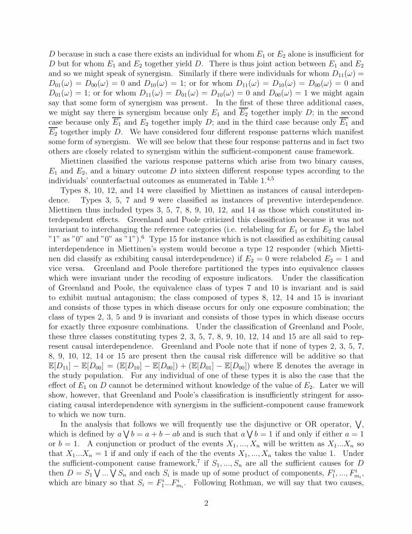
D because in such a case there exists an individual for whom E1 or E2 alone is insufficient forD but for whom E1 and E2 together yield D. There is thus joint action between E1 and E2

and so we might speak of synergism. Similarly if there were individuals for whom D11(ω) =D01(ω) = D00(ω) = 0 and D10(ω) = 1; or for whom D11(ω) = D10(ω) = D00(ω) = 0 andD01(ω) = 1; or for whom D11(ω) = D01(ω) = D10(ω) = 0 and D00(ω) = 1 we might againsay that some form of synergism was present. In the first of these three additional cases,we might say there is synergism because only E1 and E2 together imply D; in the secondcase because only E1 and E2 together imply D; and in the third case because only E1 andE2 together imply D. We have considered four different response patterns which manifestsome form of synergism. We will see below that these four response patterns and in fact twoothers are closely related to synergism within the sufficient-component cause framework.

Miettinen classified the various response patterns which arise from two binary causes,E1 and E2, and a binary outcome D into sixteen different response types according to theindividuals’ counterfactual outcomes as enumerated in Table 1.4,5

Types 8, 10, 12, and 14 were classified by Miettinen as instances of causal interdepen-dence. Types 3, 5, 7 and 9 were classified as instances of preventive interdependence.Miettinen thus included types 3, 5, 7, 8, 9, 10, 12, and 14 as those which constituted in-terdependent effects. Greenland and Poole criticized this classification because it was notinvariant to interchanging the reference categories (i.e. relabeling for E1 or for E2 the label”1” as ”0” and ”0” as ”1”).6 Type 15 for instance which is not classified as exhibiting causalinterdependence in Miettinen’s system would become a type 12 responder (which Mietti-nen did classify as exhibiting causal interdependence) if E2 = 0 were relabeled E2 = 1 andvice versa. Greenland and Poole therefore partitioned the types into equivalence classeswhich were invariant under the recoding of exposure indicators. Under the classificationof Greenland and Poole, the equivalence class of types 7 and 10 is invariant and is saidto exhibit mutual antagonism; the class composed of types 8, 12, 14 and 15 is invariantand consists of those types in which disease occurs for only one exposure combination; theclass of types 2, 3, 5 and 9 is invariant and consists of those types in which disease occursfor exactly three exposure combinations. Under the classification of Greenland and Poole,these three classes constituting types 2, 3, 5, 7, 8, 9, 10, 12, 14 and 15 are all said to rep-resent causal interdependence. Greenland and Poole note that if none of types 2, 3, 5, 7,8, 9, 10, 12, 14 or 15 are present then the causal risk difference will be additive so thatE[D11] − E[D00] = (E[D10] − E[D00]) + (E[D01] − E[D00]) where E denotes the average inthe study population. For any individual of one of these types it is also the case that theeffect of E1 on D cannot be determined without knowledge of the value of E2. Later we willshow, however, that Greenland and Poole’s classification is insufficiently stringent for asso-ciating causal interdependence with synergism in the sufficient-component cause frameworkto which we now turn.

In the analysis that follows we will frequently use the disjunctive or OR operator,∨

,which is defined by a

∨

b = a + b − ab and is such that a∨

b = 1 if and only if either a = 1or b = 1. A conjunction or product of the events X1, ..., Xn will be written as X1...Xn sothat X1...Xn = 1 if and only if each of the the events X1, ..., Xn takes the value 1. Underthe sufficient-component cause framework,7 if S1, ..., Sn are all the sufficient causes for Dthen D = S1

∨

...∨

Sn and each Si is made up of some product of components, F i1, ..., F

imi

,which are binary so that Si = F i

1...Fimi

. Following Rothman, we will say that two causes,

2

E1 and E2, for some outcome D, exhibit synergism if E1 and E2 are ever present togetherin the same sufficient cause.7,9 If E1 and E2 are present together in the same sufficientcause then the two causes E1 and E2 are said to exhibit antagonism; in this case it couldalso be said that E1 and E2 exhibit synergism. Note that E1 and E2 may exhibit bothantagonism and synergism if, for example, E1 and E2 are present together in one sufficientcause and if E1 and E2 are present together in another sufficient cause. In what followswe will not maintain the distinction between synergism and antagonism in so far as we willrefer to a sufficient cause in which both E1 and E2 are present as synergism between E1 andE2 rather than as antagonism between E1 and E2. It has become somewhat customary torefer to cases of synergism and antagonism in the sufficient-component cause framework as”biologic interactions.”10−11 This nomenclature, however, may not always be appropriate.Consider a recessive disease in which two mutant alleles convey the disease phenotype butone or zero copies of the mutant allele conveys the phenotype complement. Let E1 = 1 ifthe allele inherited from the mother is the mutant type and let E2 = 1 if the allele inheritedfrom the father is the mutant type then E1E2 is a sufficient cause for the disease because ifE1E2 = 1 then the disease will occur. Suppose that when both mutant types are present(E1E2 = 1) the disease occurs because neither allele allows for the production of an essentialprotein. Although there is synergism between E1 and E2 in the sufficient cause sense asboth E1 = 1 and E2 = 1 are necessary for the disease, there is no biological sense in whichthe two alleles are interacting. In fact neither allele is involved in any activity at all and it isprecisely this lack of action which brings about the disease. Thus, throughout this paper wewill refrain from the use of the term ”biologic interaction” and will instead refer to synergismwithin the sufficient-component cause framework. In contrast with ”biologic interaction”which suggests that causes biologically act upon each other in bringing about the outcome,the term ”synergism” suggests joint work on the outcome regardless of whether or not thecauses act on one another.

There are certain correspondences between response types and sets of sufficient causes.Greenland and Poole, in the case of two binary causes, enumerate nine different sufficientcauses each involving some combination of E1 and E2 and their complements along withcertain binary background causes.6 We may label these background causes as A0, A1, A2,A3, A4, A5, A6, A7, A8. The nine different sufficient causes Greenland and Poole give arethen A0, A1E1, A2E1, A3E2, A4E2, A5E1E2, A6E1E2, A7E1E2 and A8E1E2. Note that inthe case of the Ai and Ei variables, the subscript denotes which of the causes or backgroundfactors is being indicated whereas the subscripts for Dij denote the counterfactual outcomewith E1 set to i and E2 set to j. In many cases, not all of the nine sufficient causes willbe present. Also, if one of the background causes is unnecessary for the D (i.e. somecombination of E1, E2 and their complements are alone sufficient for D for each member ofthe population) then the corresponding background cause Ai is equal to 1 for all subjectsand we will in general suppress the Ai. Given the nine background causes, we thus havethat

D = A0

∨

A1E1

∨

A2E1

∨

A3E2

∨

A4E2

∨

A5E1E2

∨

A6E1E2

∨

A7E1E2

∨

A8E1E2. (1)

If one of A5, A6, A7, A8 were non-zero, then we would say that E1 and E2 manifest a syn-ergistic relationship. In what follows, we will assume that interventions on E1 and E2 donot affect any background causes Ai; if they did then the Ai variable would be an effect of

3

E1 and E2 rather than a background cause.12 Furthermore, if one of the Ai variable werean effect of E1 and E2 then this could obscure the identification of synergistic relationshipsbetween E1 and E2. For example, suppose that E1 and E2 together caused A0 so thatA0 = 1 whenever E1 = E2 = 1 and suppose that A0 was itself a sufficient cause for D. Thenthe A0 variable would essentially serve as a proxy for the synergism between E1 and E2. Wewill thus require that none of the Ai variables are effects of E1 and E2. It is in fact the casethat it is always possible to construct the variables A0, A1, A2, A3, A4, A5, A6, A7, A8 sothat none of the Ai variables are effects of E1 and E2 and so that equation (1) holds.13

Knowing whether there is a synergism between E1 and E2 will in general require havingsome knowledge of the causal mechanisms for the outcome D. For although a particularset of sufficient causes along with the presence or absence of the various background causesA0, A1, A2, A3, A4, A5, A6, A7, A8 for a particular individual suffices to fix a responsetype, the converse is not true.6,14 That is to say, knowledge of an individual’s response typedoes not generally fully determine which background causes are present. As an example,an individual who has A1(ω) = A3(ω) = 1 and Ai(ω) = 0 for i 6= 1, 3 has a sufficientcause completed if and only if E1 = 1 (in which case A1E1 is completed) or E2 = 1 (inwhich case A3E2 is completed). For such a individual we could write D = E1

∨

E2. Thusthis individual would be of response type 2 because the individual will escape disease only ifexposed to neither E1 nor E2 so that no sufficient cause is completed. In contrast, knowledgeof a individual’s response type does not generally fully determine which background causesare present. A individual who is of response type 2 could have either A1(ω) = A3(ω) = 1and Ai(ω) = 0 for i 6= 1, 3 in which case we could write D = E1

∨

E2 or alternatively sucha individual may have A5(ω) = A6(ω) = A7(ω) = 1 and Ai(ω) = 0 for i 6= 5, 6, 7 in whichcase we could write D = E1E2

∨

E1E2

∨

E1E2. As noted by Greenland and Brumback, itis thus impossible in this case to distinguish from the counterfactual response pattern alonethe set of sufficient causes E1

∨

E2 from the set of sufficient causes E1E2

∨

E1E2

∨

E1E2.14

With both sets of sufficient causes, D will occur when either E1 or E2 is present. WhetherE1

∨

E2 or E1E2

∨

E1E2

∨

E1E2 represent the proper description of the causal mechanismsfor D can only be resolved with knowledge of the subject matter in question.

Using the sufficient cause representation for D given above we can see that Greenlandand Poole’s classification of those types which represent causal interdependence is insuffi-ciently stringent for associating causal interdependence with synergism within the sufficient-component cause framework. Greenland and Poole include types 2, 3, 5 and 9 amongst thosetypes that are said to exhibit interdependent action. However, types 2, 3, 5 and 9 can infact be observed even when D can be represented as D = A0

∨

A1E1

∨

A2E1

∨

A3E2

∨

A4E2.For example, if A5 = A6 = A7 = A8 = 0 but if for some some individual ω, A0(ω) = A2(ω) =A4(ω) = 0 and A1(ω) = A3(ω) = 1 so that D(ω) = E1

∨

E2 then, as seen above, this wouldgive rise to response type 2. Similarly if A0(ω) = A1(ω) = A4(ω) = 0 and A2(ω) =A3(ω) = 1 then this would give rise to response type 3; if A0(ω) = A2(ω) = A3(ω) = 0 andA1(ω) = A4(ω) = 1 this would give rise to response type 5; if A0(ω) = A1(ω) = A3(ω) = 0and A2(ω) = A4(ω) = 1 this would give rise to response type 9. Response types 2, 3,5 and 9 might of course also arise from synergistic relationships. As noted above, re-sponse type 2 would arise if A0(ω) = A1(ω) = A2(ω) = A3(ω) = A4(ω) = A5(ω) = 0and A5(ω) = A6(ω) = A7(ω) = 1. Without further information concerning which causalmechanisms are present we cannot, in the case of types 2, 3, 5 and 9, ascertain from the

4

counterfactual response patterns alone whether or not a synergism is manifest. The typesthat Greenland and Poole classify as not representing causal interdependence (types 1, 4,6, 11, 13, 16) can, like types 2, 3, 5 and 9, also all be observed when D can be representedas D = A0

∨

A1E1

∨

A2E1

∨

A3E2

∨

A4E2. But all of these types, other than type 16, canalso be observed when one or more of A5, A6, A7, A8 are non-zero. In contrast, it can beshown that types 7, 8, 10, 12, 14, and 15 cannot be present when A5 = A6 = A7 = A8 = 0,i.e. when D = A0

∨

A1E1

∨

A2E1

∨

A3E2

∨

A4E2.13 These six types thus clearly do consti-

tute instances of synergism because one or more of A5, A6, A7, A8 must be non-zero for suchtypes to be present. Thus although synergistic relationships will sometimes be unidentifiedeven when the counterfactual response patterns for all individuals are known, they will notalways be unidentified. We will use the term ”definite interdependence,” which we makeprecise in Definition 1, to refer to a counterfactual response pattern which necessarily entailsa synergistic relationship.

Note that D10(ω) = D01(ω) = 0 and D11(ω) = 1 if and only if individual ω is of responsetype 7 or 8; also D11(ω) = D00(ω) = 0 and D01(ω) = 1 if and only if individual ω is ofresponse type 10 or 12; also D11(ω) = D00(ω) = 0 and D10(ω) = 1 if and only if individualω is of response type 10 or 14; and finally D01(ω) = D10(ω) = 0 and D00(ω) = 1 if andonly if individual ω is of response type 7 or 15. The presence of one of the six types thatnecessarily entail the presence of synergism is thus equivalent to the presence of an individualω for whom one of the following four conditions hold: D10(ω) = D01(ω) = 0 and D11(ω) = 1;or D11(ω) = D00(ω) = 0 and D01(ω) = 1; or D11(ω) = D00(ω) = 0 and D10(ω) = 1; orD01(ω) = D10(ω) = 0 and D00(ω) = 1. Consequently, we define definite interdependence asfollows.

Definition 1 (Definite Interdependence). Suppose that D and two of its causes, E1 and E2,are binary. We say that there is definite interdependence between the effect of E1 and E2 onD if there exists an individual ω for whom one of the following holds: D10(ω) = D01(ω) = 0and D11(ω) = 1; or D11(ω) = D00(ω) = 0 and D01(ω) = 1; or D11(ω) = D00(ω) = 0 andD10(ω) = 1; or D01(ω) = D10(ω) = 0 and D00(ω) = 1.

The definition of definite interdependence is equivalent to the presence within a popula-tion of an individual with a counterfactual response pattern of type 7, 8, 10, 12, 14, or 15. Asdefined above, if E1 and E2 exhibit definite interdependence then there must be synergismbetween E1 and E2. If D10(ω) = D01(ω) = 0 and D11(ω) = 1 then A5 6= 0 and there willbe synergism between E1 and E2. If D11(ω) = D00(ω) = 0 and D01(ω) = 1 then A6 6= 0and there will be synergism between E1 and E2. If D11(ω) = D00(ω) = 0 and D10(ω) = 1then A7 6= 0 and there will be synergism between E1 and E2. If D01(ω) = D10(ω) = 0and D00(ω) = 1 then A8 6= 0 and there will be synergism between E1 and E2. As madeclear in the discussion above, however, although definite interdependence is sufficient for asynergistic relationship, it is not necessary. There may be synergism between E1 and E2

even if they do not exhibit definite interdependence. Several related concepts have beenconsidered. In Figure 1 we give a diagram indicating the implications amongst these dif-ferent concepts. First, as noted by Greenland and Poole, effect modification on the riskdifference scale implies causal interdependence.6 Second, definite interdependence impliesboth causal interdependence (because types 7, 8, 10, 12, 14 and 15 are a subset of types

5

2, 3, 5, 7, 8, 9, 10, 12, 14 and 15) and the presence of synergism.13 No other implicationsamongst these four concepts hold.

Two additional comments with regard to definite interdependence are worth noting.First, Greenland and Poole note that there is a one-to-one correspondence between responsetypes 8, 12, 14 and 15 and ”cause types” corresponding to A5(ω) = 1, A6(ω) = 1, A7(ω) = 1and A8(ω) = 1 respectively with all other Ai(ω) = 0.6 They also note that response type16 arises if and only if Ai(ω) = 0 for all i. However, they claim that there are no otherone-to-one correspondences for the remaining 11 response types. They failed to notice thatresponse type 7 arises if and only if A5(ω) = 1 and A8(ω) = 1 with Ai(ω) = 0 for all i /∈ 5, 8and that response type 10 arises if and only if A6(ω) = 1 and A7(ω) = 1 with Ai(ω) = 0 forall i /∈ 6, 7. We will see below that this insight that response types 7 and 10 necessarilyentail a synergistic relationship is important in constructing statistical tests for the presenceof synergism.

Second, the definition of definite interdependence given above is invariant to the relabelingof the levels of E1 and E2 i.e. relabeling for E1 and/or for E2 the level ”1” as ”0” and ”0”as ”1.” Definite interdependence as defined above is not, however, invariant to the relabelingof the levels of D. If D is relabeled so that ”1” is ”0” and ”0” is ”1” then types 8, 12, 14,and 15 become types 9, 5, 3, and 2 respectively and these latter types do not exhibit definiteinterdependence. The sufficient-component cause framework (along with its philosophicalcounterpart)15 assumes that there is an asymmetry between the event and its complement inthere is a particular event or state that needs explaining. It is the event, not its complement,that requires an explanation. For example, let D denote death, let E1 denote the presenceof a gene that gives rise to a peanut allergy and let E2 denote exposure to peanuts so that ifboth E1 and E2 are present the individual will die. The event we seek to explain is death.Suppose that the lethal allergic reaction to peanuts is the only cause of death in a particulartime horizon. In this case we would represent the sufficient causes for death by D = E1E2

and since E1 and E2 are present together in the same sufficient cause we would say that E1

and E2 manifest synergism. If, however, we were considering the outcome of survival, D,then either E1 or E2 would be sufficient for averting death and the sufficient causes for notdying would be represented by D = E1

∨

E2 and no synergism between E1 and E2 would bethought to be present. We seen then that the presence of synergism for an outcome does notimply the presence of synergism for the complement of that outcome. In the example justconsidered, however, it is death not survival that requires explanation and so it is synergismfor the event of death that will be of interest.

Testing for Synergism in the Sufficient-Component Cause Framework

When there is no confounding of the causal effects of E1 and E2 on D or if there existsa set of variables C such that conditioning on C suffices to control for the confounding ofthe causal effects of E1 and E2 on D then it is possible to develop statistical tests for thepresence of synergism. Theorem 1 gives a condition which is sufficient for the presenceof synergism and which with data can be statistically tested. The proof of Theorem 1and that of Theorem 2 below are given in Appendix 1. We will say that C suffices tocontrol for the confounding of the causal effects of E1 and E2 on D if the counterfactualvariables Dij are conditionally independent of (E1, E2) given C. If this condition holds then

6

P (Dij = 1|C = c) = P (D = 1|E1 = i, E2 = j, C = c).

Theorem 1. Suppose that D and two of its causes, E1 and E2, are binary. Let C be a set ofvariables that suffices to control for the confounding of the causal effects of E1 and E2 on Dthen if for any value c of C we have that P (D = 1|E1 = 1, E2 = 1, C = c) − P (D = 1|E1 =0, E2 = 1, C = c)−P (D = 1|E1 = 1, E2 = 0, C = c) > 0 then there is synergism between E1

and E2.

When the condition of Theorem 1 is met, an individual of either type 7 or type 8 must bepresent and from the discussion above it follows that there must be synergism between E1

and E2. Theorem 1 has analogues for testing for synergism between E1 and E2 or betweenE1 and E2 or between E1 and E2. If for some c, P (D = 1|E1 = 1, E2 = 0, C = c) − P (D =1|E1 = 1, E2 = 1, C = c) − P (D = 1|E1 = 0, E2 = 0, C = c) > 0 then an individual oftype 10 or type 14 must be present and there will be synergism between E1 and E2. IfP (D = 1|E1 = 0, E2 = 1, C = c)−P (D = 1|E1 = 1, E2 = 1, C = c)−P (D = 1|E1 = 0, E2 =0, C = c) > 0 then an individual of type 10 or type 12 must be present and there will besynergism between E1 and E2. If P (D = 1|E1 = 0, E2 = 0, C = c)−P (D = 1|E1 = 0, E2 =1, C = c)−P (D = 1|E1 = 1, E2 = 0, C = c) > 0 then an individual of type 7 or type 15 mustbe present and there will be synergism between E1 and E2. Theorem 1 and its analoguesdemonstrate that the claim of Rothman and Greenland that ”inferences about the presenceof particular response types or sufficient causes must depend on very restrictive assumptionsabout absence of other response types” (p. 339) is false.11 Although their claim holds forinference about particular response types, Theorem 1 demonstrates that it does not hold forinferences about sufficient causes. Theorem 1 makes no assumption about the absence ofany response type.

It is interesting to note that Theorem 1 does not make reference to probability of theoutcome D when E1 and E2 are both 0 i.e. to P (D = 1|E1 = 0, E2 = 0, C = c). Thecondition of Theorem 1 essentially ensures the presence of some individual ω for whomD11(ω) = 1 and for whom D10(ω) = D01(ω) = 0. For such an individual, if D00(ω) = 0then individual ω is of type 8; if D00(ω) = 1 then individual ω is of type 7. Theorem 1does not distinguish between types 7 and 8; the conclusion of the theorem simply impliesthat an individual of one of these two types must be present and thus that there must besynergism between E1 and E2. Whether individual is ω of type 7 or type 8 will affect theprobability P (D = 1|E1 = 0, E2 = 0, C = c) but it will not affect the probability involved inthe condition given in Theorem 1, namely P (D = 1|E1 = 1, E2 = 1, C = c)−P (D = 1|E1 =0, E2 = 1, C = c) − P (D = 1|E1 = 1, E2 = 0, C = c).

We consider an example concerning the effects of smoking and asbestos on lung cancer.For the purpose of this example we will ignore sampling variability. Suppose that the rateratios for lung cancer given smoking status S and asbestos exposure A are given in Table2. Let Rij be the risk (i.e. cumulative incidence) of lung cancer before age 60 if smokingstatus S is i and asbestos exposure A is j and let RRij be the relative risk of lung cancerbefore age 60 for individuals with S = i and A = j as compared to lung cancer risk forindividuals unexposed to smoking and asbestos. Since in all smoking-asbestos categoriesthe risk of lung cancer before age 60 is small, the risk ratio RRij closely approximatesthe rate ratios in Table 2. Suppose that the data is unconfounded by other factors so

7

that Rij = P (D = 1|S = i, A = j). The condition of Theorem 1 may be written asR11 − R01 − R10 > 0. By dividing this condition by R00 the condition can be re-written asRR11 − RR01 − RR10 > 0. In this case, RR11 − RR01 − RR10 = 30 − 3 − 10 = 17 > 0.We could thus conclude that synergism was present in the sufficient cause sense betweensmoking and asbestos exposure. Note that the conclusion of the presence of synergism inthe sufficient cause sense holds in spite of the fact that the multiplicative risk model holdsi.e. RR11 = RR01RR10. Note further that the conclusion of the presence of synergism inthe sufficient cause sense did not preclude cases in which one or both factors are sometimespreventive. For example, for certain individuals exposure to asbestos might protect againstlung cancer. This might be the case if (i) there exist individuals who carry a very low riskof smoking induced cancer due to a genetic polymorphism but who still suffer from smoking-induced chronic bronchitis and (ii) the narrowed airways and increased mucous caused bytheir bronchitis trap and eliminate asbestos fibers that would have otherwise reached the lungparenchyma. Theorem 1 can still be applied to such cases. The example of course is rathersimplified in that smoking and asbestos exposure are better captured by continuous ratherthan binary measures. The difficulties which continuous variables pose to the sufficient-component cause framework is taken up in the discussion section. Also, in practice, withfinite samples, one must use various statistical tests and methods of statistical inference inorder to determine whether the condition given in Theorem 1 holds. One such statisticaltest is given in Appendix 2. Such tests can be used empirically with epidemiologic data totest for synergism in the sufficient-component cause framework. Limitations of such testsare discussed at the paper’s conclusion.

Testing for Synergism under the Assumption of Monotonic Effects

We next consider a context in which the direction of the effect (positive or negative) thatE1 and E2 have on D is known. We make these ideas precise by introducing the conceptof a monotonic effect. Considerable intuition regarding synergism can be garnered by theconsideration of the setting of monotonic effects. Furthermore, as will be seen shortly,the setting of monotonic effects also allows for the construction of more powerful tests fordetecting synergism than is possible without the assumption.

Definition 2 (Monotonic Effect): We will say that E1 has a positive monotonic effect onD if for all individuals ω we have Dij(ω) ≥ Di′j(ω) whenever i ≥ i′; we will say that E2

has a positive monotonic effect on D if for all individuals ω we have Dij(ω) ≥ Dij′(ω)whenever j ≥ j′. Similarly, we will say that E1 has a negative monotonic effect on D iffor all individuals ω we have Dij(ω) ≤ Di′j(ω) whenever i ≥ i′ and that E2 has a negativemonotonic effect on D if for all individuals ω we have Dij(ω) ≤ Dij′(ω) whenever j ≥ j′.

The definition of a monotonic effect essentially requires that some intervention eitherincrease or decrease some other variable D not merely on average over the entire popula-tion but rather for every individual in that population regardless of the other intervention.The requirements for the attribution of a monotonic effect are thus considerable. Howeverwhenever a particular intervention is always beneficial or neutral for all individuals, there isa positive monotonic effect; whenever the intervention is always harmful or neutral for allindividuals, there is a negative monotonic effect. The assumption of monotonic effects has

8

been used elsewhere in the context of concepts of interaction,9,11,12,16 and it is sometimesreferred to as an assumption of ”no preventive effects” or purely ”causative factors.” It canbe shown that E1 has a positive monotonic effect on D if and only if E1 is not present inany sufficient cause. Similarly, E1 has a negative monotonic effect on D if and only if E1 isnot present in any sufficient cause (though E1 may still be present).

Theorem 2 gives a result similar to that of Theorem 1 but under the assumption thatboth E1 and E2 have positive monotonic effects on D.

Theorem 2. Suppose that D and two of its causes, E1 and E2, are binary and that E1 andE2 have a positive monotonic effect on D. Let C be a set of variables that suffices to controlfor the confounding of the causal effects of E1 and E2 on D then if for any value c of C wehave that P (D = 1|E1 = 1, E2 = 1, C = c) − P (D = 1|E1 = 0, E2 = 1, C = c) > P (D =1|E1 = 1, E2 = 0, C = c)−P (D = 1|E1 = 0, E2 = 0, C = c) then there is synergism betweenE1 and E2.

The condition provided in Theorem 2 has obvious analogues if one or both of E1 andE2 are replaced by E1 and E2 respectively and if one or both of E1 and E2 have a negativemonotonic effect rather than a positive monotonic effect on D. If the condition of Theorem2 is met, an individual of type 8 must be present. Individuals of type 7, the other type thatentails synergism between E1 and E2, are precluded because E1 has a positive monotoniceffect on D (and similarly because E2 has a positive monotonic effect on D). Rothman andGreenland note the equivalent result in the setting of no confounding factors.11 A statisticaltest for the condition of Theorem 2 is given in Appendix 2. As noted above, such tests canbe used empirically with epidemiologic data to test for synergism in the sufficient-componentcause framework. Note that the general condition of Theorem 1 for detecting the presenceof synergism between E1 and E2, P (D = 1|E1 = 1, E2 = 1, C = c) − P (D = 1|E1 =0, E2 = 1, C = c) − P (D = 1|E1 = 1, E2 = 0, C = c) > 0, is stronger than the condition,P (D = 1|E1 = 1, E2 = 1, C = c)−P (D = 1|E1 = 0, E2 = 1, C = c)−P (D = 1|E1 = 1, E2 =0, C = c)+P (D = 1|E1 = 0, E2 = 0, C = c) > 0, required in the setting of monotonic effects.Indeed the former clearly implies the latter. The statistical tests based on this condition inthe setting of monotonic effects will thus be more powerful than the equivalent tests in thegeneral setting.

Effect Modification and Synergism

Theorem 2 suggests the risk difference scale as the means by which to test for synergismin the presence of monotonic effects. As will be seen below and as has been pointed outbefore, effect modification on the risk difference scale need not imply any form of synergy.Furthermore, in the presence of confounding, effect modification on the risk difference scaleneed not even imply the modification of an actual causal effect. Nevertheless, Theorem 2can be interpreted as stating that, conditional on confounding factors, if the risk differencefor E1 in the strata E2 = 1 is greater than the risk difference for E1 in the strata E2 = 0 thenE1 and E2 must exhibit synergism. The condition can also be re-written as P (D = 1|E1 =1, E2 = 1, C = c) − P (D = 1|E1 = 0, E2 = 0, C = c) > P (D = 1|E1 = 0, E2 = 1, C =c) − P (D = 1|E1 = 0, E2 = 0, C = c) + P (D = 1|E1 = 1, E2 = 0, C = c) − P (D = 1|E1 =0, E2 = 0, C = c) i.e. the effect of E1 and E2 is greater than the sum of the effects of E1 and

9

E2 separately. The result is in many ways intuitive and not at all surprising. Nevertheless,several distinctions between the categories of effect modification on the risk difference scaleand that of definite interdependence or synergism must be kept in mind however. We givenumerical examples in Appendix 3 to demonstrate the following observations. First, itis possible to have effect modification on the risk difference scale without the presence ofsynergism in the sufficient-component cause framework (see Appendix 3, Numerical Example1). This may arise when the effect modification is in the opposite direction of that requiredby Theorem 2.

Second, it is furthermore the case that the absence of effect modification on the riskdifference scale does not imply the absence of synergism. In other words, if P (D = 1|E1 =1, E2 = 1, C = c) − P (D = 1|E1 = 0, E2 = 1, C = c) > P (D = 1|E1 = 1, E2 = 0, C =c) − P (D = 1|E1 = 0, E2 = 0, C = c) then there must be synergism but even if P (D =1|E1 = 1, E2 = 1, C = c) − P (D = 1|E1 = 0, E2 = 1, C = c) ≤ P (D = 1|E1 = 1, E2 =0, C = c) − P (D = 1|E1 = 0, E2 = 0, C = c) there may yet be a synergistic relationship(see Appendix 3, Numerical Example 2). Thus, Theorem 2 gives a condition (in terms ofeffect modification on the risk difference scale) which, in the setting of monotonic effects, issufficient for synergism but not necessary. Third, if it is not the case that both E1 and E2

have a monotonic effect on D then we may have P (D = 1|E1 = 1, E2 = 1) − P (D = 1|E1 =0, E2 = 1) > P (D = 1|E1 = 1, E2 = 0) − P (D = 1|E1 = 0, E2 = 0) even when there is nosynergism and furthermore in such cases we can also have E2 acting as a qualitative effectmodifier for the risk difference of E1 on D without E1 and E2 manifesting synergism (seeAppendix 3, Numerical Example 3).

These comments and the three numerical examples in the Appendix thus help clarify theconceptual distinction between effect modification on the risk difference scale and synergism,even in the presence of monotonic effects. There can be effect modification on the riskdifference scale without the presence of synergism. There can be synergism without therisk difference condition P (D = 1|E1 = 1, E2 = 1, C = c) − P (D = 1|E1 = 0, E2 = 1, C =c) > P (D = 1|E1 = 1, E2 = 0, C = c) − P (D = 1|E1 = 0, E2 = 0, C = c) holding. And,finally, outside the context of monotonic effects, we may have P (D = 1|E1 = 1, E2 = 1, C =c) − P (D = 1|E1 = 0, E2 = 1, C = c) > P (D = 1|E1 = 1, E2 = 0, C = c) − P (D = 1|E1 =0, E2 = 0, C = c) without the presence of synergism.

Discussion

The present work has extended the literature on the relationship between counterfactualresponse types and the concept of synergism in the sufficient-component cause framework.The paper contributes substantially to the conceptual literature on synergism and providesnovel tests for detecting synergistic relationships. The specific contributions of the paper areas follows. First, we have provided a complete characterization, in the context of two binarycauses, of those response types that necessarily entail synergism in the sufficient-componentcause framework; the collection of these response types we have given the label ”definiteinterdependence.” Second, this characterization has allowed for the derivation of empiricalconditions which, under the assumption of no unmeasured confounders, necessarily entail thepresence of synergism (Theorems 1 and 2). Theorem 2, in the context of monotonic effects,is a straightforward generalization of previous results in the literature. However, Theorem 1,

10

which makes no assumptions about the absence of certain response types, is entirely novel.These results can be used to empirically test for synergism in the sufficient-component causeframework. Third, we have illustrated through a series of numerical examples in Appendix3 the distinction between the concept of effect modification on the risk difference scale andthe conditions which necessarily entail the presence of synergism.

Several issues merit further attention. First, it is to be noted that the sufficient-component cause framework is limited in an important respect: it is restricted to binaryvariables (or variables that can be re-coded as binary variables). Thus in biologic sys-tems governing continuous variables the concept of synergism arising from the sufficient-component cause framework is not applicable. Note that it has also been pointed out thatwith continuous variables it furthermore becomes difficult to separate assumptions aboutinteraction from those of induction time and dose-response.17−18 Second, the tests for syn-ergism could be extended to the case of three or more variables. We have addressed thisextension in related research.13 Third, the discussion in the paper has assumed a deter-

ministic counterfactual and sufficient-component cause setting. Relationships between astochastic counterfactual setting (wherein each individual has a certain probability of dis-ease under each of the four exposure combinations) and stochastic sufficient causes (whereinwhen a sufficient cause is completed, the individual has a certain probability of the outcome)could also be considered. Finally, our focus has been conceptual, with relatively little at-tention given to applied data analysis. It has been noted elsewhere that the power for testsof interaction are often low in many study settings.19 Further work remains to be done inexamining whether the statistical tests derived in this paper could be usefully employed inactual studies. Recent studies in genetics with regard to gene-gene and gene-environmentinteractions might be a fruitful area in which to examine the potential utility of these tests.

Appendix 1. Proofs.

Proof of Theorem 1.

Suppose that for some set of variables V , E[D11 −D01 −D10|V = v] > 0 then there must besome individual ω for whom V = v and D11(ω) = 1 but D01(ω) = D10(ω) = 0 for if one ofD01(ω), D10(ω) were always 1 whenever D11(ω) = 1 then D11(ω) − D01(ω) − D10(ω) wouldbe less than or equal to zero for all ω and so we would have that E[D11 − D01 − D10|V =v] ≤ 0. Let V = C. The condition E[D11 − D01 − D10|C = c] > 0 implies definiteinterdependence and thus the presence of synergism. Because C is a set of variables thatsuffices to control for the confounding of the causal effects of E1 and E2 on D we have thatthe counterfactual variables Dij are conditionally independent of (E1, E2) given C. Thus wehave, E[D11−D01−D10|C = c] = E[D11|E1 = 1, E2 = 1, C = c]−E[D01|E1 = 0, E2 = 1, C =c] − E[D10|E1 = 1, E2 = 0, C = c] = P (D = 1|E1 = 1, E2 = 1, C = c) − P (D = 1|E1 =0, E2 = 1, C = c) − P (D = 1|E1 = 1, E2 = 0, C = c). Consequently, if P (D = 1|E1 =1, E2 = 1, C = c) − P (D = 1|E1 = 0, E2 = 1, C = c) − P (D = 1|E1 = 1, E2 = 0, C = c) > 0then E1 and E2 must exhibit synergism.

Proof of Theorem 2.

We first show that if for some set of variables V , E[(D11 − D01) − (D10 − D00)|V = v] > 0for some v then there must be synergism. For each individual ω define B0(ω), B1(ω), B2(ω)

11

and B3(ω) as follows: B0(ω) = 1 if D00(ω) = 1 and 0 otherwise; B1(ω) = 1 if D10(ω) = 1and 0 otherwise; B2(ω) = 1 if D01(ω) = 1 and 0 otherwise; and B3(ω) = 1 if D11(ω) = 1 andD10(ω) = D01(ω) = 0 and 0 otherwise. Then D00 = B0, D10 = B0

∨

B1, D01 = B0

∨

B2,D11 = B0

∨

B1

∨

B2

∨

B3. Suppose there is no synergism between E1 and E2; then B3(ω) =0 for all ω ∈ Ω so that D11 = B0

∨

B1

∨

B2. Let P (B0|V = v) = bv0, P (B1|V = v) = bv

1,P (B2|V = v) = bv

2, P (B0B1|V = v) = bv01, P (B0B2|V = v) = bv

02, P (B1B2|V = v) = bv12 and

P (B0B1B2|V = v) = bv012. Then P (B0|V = v) = bv

0; P (B0

∨

B1|V = v) = bv0 + bv

1 − bv01;

P (B0

∨

B2|V = v) = bv0+bv

2−bv02; P (B0

∨

B1

∨

B2|V = v) = bv0+bv

1+bv2−(bv

01+bv02+bv

12)+bv012.

E[(D11 − D01) − (D10 − D00)|V = v] = P (B0

∨

B1

∨

B2|V = v) − P (B0

∨

B2|V = v) −P (B0

∨

B1|V = v) − P (B0|V = v) = [bv0 + bv

1 + bv2 − (bv

01 + bv02 + bv

12) + bv012 − bv

0 +bv2 − bv

02] − [bv0 + bv

1 − bv01 − bv

0] = (bv012 − bv

12 + bv1 − bv

01) − (bv1 − bv

01) = bv012 − bv

12 < 0.Thus if E[(D11 − D01) − (D10 − D00)|V = v] > 0 we cannot have B3(ω) = 0 for all ωand so there must be synergism between E1 and E2. Now let V = C then we have thatsynergism is implied by the condition E[(D11 − D01) − (D10 − D00)|C = c] > 0. BecauseC is a set of variables that suffices to control for the confounding of the causal effects of E1

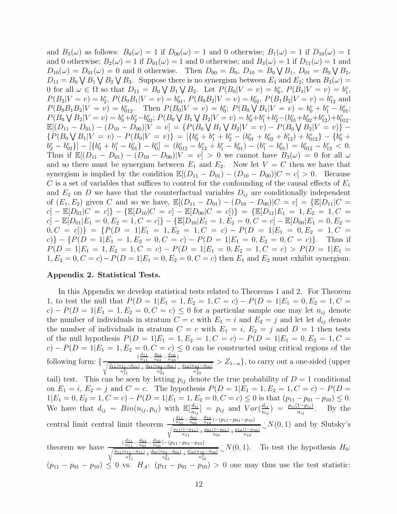
and E2 on D we have that the counterfactual variables Dij are conditionally independentof (E1, E2) given C and so we have, E[(D11 − D01) − (D10 − D00)|C = c] = E[D11|C =c] − E[D01|C = c] − E[D10|C = c] − E[D00|C = c]) = E[D11|E1 = 1, E2 = 1, C =c] − E[D01|E1 = 0, E2 = 1, C = c] − E[D10|E1 = 1, E2 = 0, C = c] − E[D00|E1 = 0, E2 =0, C = c]) = P (D = 1|E1 = 1, E2 = 1, C = c) − P (D = 1|E1 = 0, E2 = 1, C =c) − P (D = 1|E1 = 1, E2 = 0, C = c) − P (D = 1|E1 = 0, E2 = 0, C = c). Thus ifP (D = 1|E1 = 1, E2 = 1, C = c) − P (D = 1|E1 = 0, E2 = 1, C = c) > P (D = 1|E1 =1, E2 = 0, C = c)−P (D = 1|E1 = 0, E2 = 0, C = c) then E1 and E2 must exhibit synergism.

Appendix 2. Statistical Tests.

In this Appendix we develop statistical tests related to Theorems 1 and 2. For Theorem1, to test the null that P (D = 1|E1 = 1, E2 = 1, C = c) − P (D = 1|E1 = 0, E2 = 1, C =c) − P (D = 1|E1 = 1, E2 = 0, C = c) ≤ 0 for a particular sample one may let nij denotethe number of individuals in stratum C = c with E1 = i and E2 = j and let let dij denotethe number of individuals in stratum C = c with E1 = i, E2 = j and D = 1 then testsof the null hypothesis P (D = 1|E1 = 1, E2 = 1, C = c) − P (D = 1|E1 = 0, E2 = 1, C =c) − P (D = 1|E1 = 1, E2 = 0, C = c) ≤ 0 can be constructed using critical regions of the

following form: (

d11n11

−d01n01

−d10n10

)√

d11(n11−d11)

n311

+d01(n01−d01)

n301

+d10(n10−d10)

n310

> Z1−α, to carry out a one-sided (upper

tail) test. This can be seen by letting pij denote the true probability of D = 1 conditionalon E1 = i, E2 = j and C = c. The hypothesis P (D = 1|E1 = 1, E2 = 1, C = c) − P (D =1|E1 = 0, E2 = 1, C = c)−P (D = 1|E1 = 1, E2 = 0, C = c) ≤ 0 is that (p11 − p01 − p10) ≤ 0.

We have that dij ∼ Bin(nij , pij) with E[dij

nij] = pij and V ar(

dij

nij) =

pij(1−pij)

nij. By the

central limit central limit theorem(

d11n11

−d01n01

−d10n10

)−(p11−p01−p10)√

p11(1−p11)n11

+p01(1−p01)

n01+

p10(1−p10)n10

.

∼N(0, 1) and by Slutsky’s

theorem we have(

d11n11

−d01n01

−d10n10

)−(p11−p01−p10)√

d11(n11−d11)

n311

+d01(n01−d01)

n301

+d10(n10−d10)

n310

.

∼N(0, 1). To test the hypothesis H0:

(p11 − p01 − p10) ≤ 0 vs. HA: (p11 − p01 − p10) > 0 one may thus use the test statistic:

12

(d11n11

−d01n01

−d10n10

)√

d11(n11−d11)

n311

+d01(n01−d01)

n301

+d10(n10−d10)

n310

.

If C consists of a small number of binary or categorical variables then it may be possibleto use the tests constructed above to test all strata of C. When C includes a continuousvariable or many binary and categorical variables such testing becomes difficult because thedata in certain strata of C will be sparse. One might then model the conditional probabilitiesP (D = 1|E1, E2, C) using a binomial or Poisson regression model with a linear link.20−24 Forcase-control studies it will be necessary to use an adapted set of modeling techniques.23,25,26

The condition of Theorem 2 can be tested in a manner analogous to the condition ofTheorem 1. In general to test the null that P (D = 1|E1 = 1, E2 = 1, C = c)−P (D = 1|E1 =0, E2 = 1, C = c) ≤ P (D = 1|E1 = 1, E2 = 0, C = c) − P (D = 1|E1 = 0, E2 = 0, C = c) fora particular sample, tests of the null hypothesis can be constructed using critical regions of

the following form: (

d11n11

−d01n01

)−(d10n10

−d00n00

)√

d11(n11−d11)

n311

+d01(n01−d01)

n301

+d10(n10−d10)

n310

++d00(n00−d00)

n300

> Z1−α.

Appendix 3. Numerical Examples for Effect Modification, Definite Interdepen-

dence and the Multiplicative Survival Model.

This appendix presents three computational examples illustrating the difference betweeneffect modification on the risk difference scale and the concepts of definite interdependenceand synergism. Recall, effect modification on the risk difference scale is said to be presentif P (D = 1|E1 = 1, E2 = e2) − P (D = 1|E1 = 0, E2 = e2) varies with the value of e2. Inthe absence of confounding this is also equal to the causal risk difference E(D1e2)−E(D0e2).Definite interdependence between E1 and E2 is said to be manifest if every sufficient causerepresentation for D must have a sufficient cause in which both E1 and E2 (or one or boththeir complements) are present. There is said to be synergism between E1 and E2 if thesufficient cause representation that corresponds to the actual causal mechanisms for D hasa sufficient cause in which both E1 and E2 are present.

Numerical Example 1. We show that effect modification of the risk difference may bepresent without definite interdependence or synergism. Suppose that D, E1 and E2 arebinary and that D = A0

∨

A1E1

∨

A2E2. Then E1 and E2 have a positive monotonic effecton D and E1 and E2 do not exhibit definite interdependence. Suppose further that thecausal effects of E1 and E2 on D are unconfounded. Let P (A0) = a0, P (A1) = a1, P (A2) =a2, P (A0A1) = a01, P (A0A2) = a02, P (A1A2) = a12, P (A0A1A2) = a012. We then haveP (D = 1|E1 = 0, E2 = 0) = P (A0) = a0; P (D = 1|E1 = 1, E2 = 0) = P (A0

∨

A1) =a0 + a1 − a01; P (D = 1|E1 = 0, E2 = 1) = P (A0

∨

A2) = a0 + a2 − a02; and P (D =1|E1 = 1, E2 = 1) = P (A0

∨

A1

∨

A2) = a0 + a1 + a2 − a01 − a02 − a12 + a012. Conditionalon E2 = 0, the risk difference for E1 is given by: P (D = 1|E1 = 1, E2 = 0) − P (D =1|E1 = 0, E2 = 0) = a0 + a1 − a01 − a0 = a1 − a01. Conditional on E2 = 1, the riskdifference for E1 is given by: P (D = 1|E1 = 1, E2 = 1) − P (D = 1|E1 = 0, E2 = 1) =a0+a1+a2−a01−a02−a12 +a012−(a0 +a2−a02) = (a1−a01)−(a12−a012). In this example,P (D = 1|E1 = 1, E2 = 1)−P (D = 1|E1 = 0, E2 = 1) = (a1−a01)− (a12 −a012) 6= a1−a01 =P (D = 1|E1 = 1, E2 = 0) − P (D = 1|E1 = 0, E2 = 0). We see then from this example thatwe can have effect modification on the risk difference scale (”statistical interaction”) even

13

when no synergism (or antagonism) is present. This will occur whenever (a12 − a012) 6= 0i.e. when P (A1A2) 6= P (A0A1A2) or equivalently P (A0 = 1|A1 = 1, A2 = 1) < 1.

Numerical Example 1 also sheds light on the conditions under which a multiplicativesurvival model can be used to test for synergism. The multiplicative survival model is saidto hold when P (D = 0|E1 = 1, E2 = 1)P (D = 0|E1 = 0, E2 = 0) = P (D = 0|E1 = 1, E2 =0)P (D = 0|E1 = 0, E2 = 1). In Example 1, the probabilities of survival are: P (D = 0|E1 =0, E2 = 0) = 1−a0; P (D = 0|E1 = 0, E2 = 1) = 1−a0−a1+a01; P (D = 0|E1 = 0, E2 = 1) =1−a0−a2 +a02; P (D = 0|E1 = 1, E2 = 1) = 1−a0−a1−a2 +a01 +a02 +a12−a012 and thus:P (D = 0|E1 = 1, E2 = 1)P (D = 0|E1 = 0, E2 = 0) = (1− a0)(1− a0 − a1 − a2 + a01 + a02 +a12−a012) = 1−a0−a1−a2+a01+a02+a12−a012−a0(1−a0−a1−a2+a01+a02+a12−a012); butP (D = 0|E1 = 1, E2 = 0)P (D = 0|E1 = 0, E2 = 1) = (1− a0 − a1 + a01)(1− a0 − a2 + a02) =1−a0−a1 +a01−a0−a2+a02 +a2

0+a0a2−a0a02+a0a1+a1a2−a1a02−a0a01−a2a01+a01a02;.Thus, P (D = 0|E1 = 1, E2 = 1)P (D = 0|E1 = 0, E2 = 0)−P (D = 0|E1 = 1, E2 = 0)P (D =0|E1 = 0, E2 = 1) = (a12 − a1a2) − (a012 − a1a02) − (a0a12 − a2a01) + (a0a012 − a01a02) 6= 0which will generally be non-zero so the multiplicative survival model will fail to hold inthis example. However, if A0, A1 and A2 were independently distributed then the aboveexpression is zero and the multiplicative survival model holds. Somewhat more generally, ifA1 and A2 were independent of one another and also either A1 or A2 were independent of A0

then the expression would again be zero and the multiplicative survival model would hold.Greenland and Poole proposed the multiplicative survival model as a means to assess theinterdependence versus the independence of causal effects under the setting that the ”effectsof exposures are probabilistically independent of any background causes, as well as of oneanother’s effect.”6 Example 1 underscores the necessity for the background causes to alsobe independent of one another when using the multiplicative survival model to detect thepresence of synergism. More precisely, we have shown that if E1 and E2 have a positivemonotonic effect on D and if A1 and A2 are independent of one another and either A1 orA2 is independent of A0 then the multiplicative survival model will hold when there is nosynergism between E1 and E2. Therefore, if, under these assumptions, the multiplicativesurvival model does not hold then one could conclude that synergism was present between E1

and E2. Consideration of the use of the multiplicative survival model to test for interactionsregarding biologic mechanisms is also given elsewhere.12,16

Numerical Example 2. We show that synergism may be present without effect modi-fication of the risk difference. Suppose that D, E1 and E2 are binary, that E1 and E2

are independent and that D = A0

∨

A1E1

∨

A2E2

∨

A3E1E2. Then E1 and E2 have apositive monotonic effect on D and E1 and E2 do exhibit synergism. Suppose furtherthat the causal effects of E1 and E2 on D are unconfounded. Let P (A0) = a0, P (A1) =a1, P (A2) = a2, P (A3) = a3, P (A0A1) = a01, P (A0A2) = a02, ..., P (A0A1A2A3) = a0123.We then have P (D = 1|E1 = 0, E2 = 0) = P (A0) = a0; P (D = 1|E1 = 1, E2 = 0) =P (A0

∨

A1) = a0 + a1 − a01; P (D = 1|E1 = 0, E2 = 1) = P (A0

∨

A2) = a0 + a2 − a02;and P (D = 1|E1 = 1, E2 = 1) = P (A0

∨

A1

∨

A2) = (a0 + a1 + a2 + a3) − (a01 + a02 +a03 + a12 + a13 + a23) + (a012 + a013 + a023 + a123) − a0123. Thus P (D = 1|E1 = 1, E2 =1) − P (D = 1|E1 = 0, E2 = 1) − P (D = 1|E1 = 1, E2 = 0) + P (D = 1|E1 = 0, E2 = 0) =(a012−a12)+a3−(a03+a13+a23)+(a013+a023+a123)−a0123. Suppose now that with probability

14

0.5, A0 = 0, A1 = 0, A2 = 0, A3 = 1 and with probability 0.5, A0 = 0, A1 = 1, A2 = 1, A3 = 0so that a3 = 0.5 and a12 = 0.5 and a012 = a03 = a13 = a23 = a013 = a023 = a123 = a0123 = 0then P (D = 1|E1 = 1, E2 = 1) − P (D = 1|E1 = 0, E2 = 1) − P (D = 1|E1 = 1, E2 =0) + P (D = 1|E1 = 0, E2 = 0) = a3 − a12 = 0.5 − 0.5 = 0 and so although synergism ispresent the inequality P (D = 1|E1 = 1, E2 = 1) − P (D = 1|E1 = 0, E2 = 1) > P (D =1|E1 = 1, E2 = 0) − P (D = 1|E1 = 0, E2 = 0) fails to hold. The example demonstratesthat although the inequality is a sufficient condition for synergism under the setting ofmonotonic effects, it is not necessary. It is also interesting to note that in this exampleP (D = 1|E1 = 1, E2 = 1) − P (D = 1|E1 = 0, E2 = 1) − P (D = 1|E1 = 1, E2 = 0) + P (D =1|E1 = 0, E2 = 0) = a3 − (a03 + a13 + a23) + (a013 + a023 + a123) − a0123 − (a12 − a012)and this final expression can be rewritten as P (A3A0A1A2) − P (A1A2A0) suggesting thatthe more likely that A3 occurs when A0, A1, A2 are absent, the more power the test impliedby Theorem 2 will have to detect the synergism; on the other hand the more likely that A1

and A2 occur together when A0 is absent, the less power the test implied by Theorem 2 willhave to detect the synergism.

The contrast between Examples 1 and 2 is interesting. Example 1 demonstrated thateffect modification could be present without synergism. In Example 1, effect modification onthe risk difference scale would be present whenever P (A1A2) 6= P (A0A1A2) suggesting that,in general, effect modification on the risk difference scale may be present without synergismif the various background causes A0, A1 and A2 can occur simultaneously i.e. when multiplecausal mechanisms may be simultaneously operative. It is, of course, also possible to haveeffect modification that is attributable solely to synergism rather than to the backgroundcauses. Example 2 considered the general case of synergism between E1 and E2 under thesetting of monotonic effects. The expression for P (D = 1|E1 = 1, E2 = 1)−P (D = 1|E1 =0, E2 = 1) − P (D = 1|E1 = 1, E2 = 0) − P (D = 1|E1 = 0, E2 = 0) could be rewritten as(a012 − a12) + (a3 − a03 − a13 − a23 + a013 + a023 + a123 − a0123). For no effect modificationon the risk difference scale to be present in Example 2 the sum of these two terms wouldhave to be zero. Note that each part of the second term involves the subscript 3. Thesecond term can thus be seen as the synergistic component; it will be zero when A3 = 0.We saw in Example 1 that the first term being zero, (a012 − a12) = 0, was the condition forno effect modification in the case of A3 = 0. Suppose that (a012 − a12) = 0 but A3 6= 0and (a3 − a03 − a13 − a23 + a013 + a023 + a123 − a0123) 6= 0 then the effect modification inExample 2 would be attributable solely to synergism (i.e. no effect modification would bepresent if A3 = 0). Thus in Example 1, the effect modification was wholly attributableto the possibility of the background causes A0, A1 and A2 occurring simultaneously and inExample 2, if (a012 − a12) = 0, the effect modification would be wholly attributable to thepresence of synergism. In general, effect modification may arise either due to backgroundcauses or due to the presence of synergism or due to both.

Numerical Example 3. We show that without monotonic effects, one may have ”super-additive” effect modification of the risk difference without definite interdependence or syn-ergism. Suppose that D, E1 and E2 are binary, that E1 and E2 are independent andthat D = A1E1

∨

A2E1

∨

A3E2. Then E1 and E2 do not exhibit definite interdepen-dence. Suppose further that the causal effects of E1 and E2 on D are unconfounded.

15

Finally, suppose that with probability 0.3, A1 = 1, A2 = 0, A3 = 1; with probability 0.3,A1 = 1, A2 = 0, A3 = 0; and with probability 0.4, A1 = 0, A2 = 1, A3 = 0 so that a1 = 0.6,a2 = 0.4, a3 = 0.3, a13 = 0.3 and a23 = 0. We then have P (D = 1|E1 = 0, E2 = 0) =P (A2

∨

A3) = a2 + a3 − a23; P (D = 1|E1 = 1, E2 = 0) = P (A1

∨

A3) = a1 + a3 − a13;P (D = 1|E1 = 0, E2 = 1) = P (A2) = a2; and P (D = 1|E1 = 1, E2 = 1) = P (A1) = a1.Conditional on E2 = 0, the risk difference for E1 is given by: P (D = 1|E1 = 1, E2 =0) − P (D = 1|E1 = 0, E2 = 0) = a1 + a3 − a13 − (a2 + a3 − a23) = a1 − a2 − a13 + a23 =0.6 − 0.4 − 0.3 = −0.1. Conditional on E2 = 1, the risk difference for E1 is given by:P (D = 1|E1 = 1, E2 = 1) − P (D = 1|E1 = 0, E2 = 1) = a1 − a2 = 0.6 − 0.4 = 0.2. In thisexample, P (D = 1|E1 = 1, E2 = 1) − P (D = 1|E1 = 0, E2 = 1) > P (D = 1|E1 = 1, E2 =0)−P (D = 1|E1 = 0, E2 = 0) but no synergism was present. We see also from this examplethat we can have qualitative effect modification even when no synergism is present.

References

1. Blot WJ, Day NE. Synergism and interaction: are they equivalent? Am. J. Epidemiol.

1979;100:99-100.

2. Rothman KJ, Greenland S, Walker AM. Concepts of interaction. Am. J. Epidemiol.

1980;112:467-470.

3. Saracci R. Interaction and synergism. Am. J. Epidemiol. 1980;112:465-466.

4. Miettinen OS. Causal and preventive interdependence: Elementary principles. Scand. J.

Work Environ. Health 1982;8:159-168.

5. Miettinen OS. Modern Epidemiology. New York: John Wiley; 1985.

6. Greenland S, Poole C. Invariants and noninvariants in the concept of interdependenteffects. Scand. J. Work Environ. Health 1988;14:125-129.

7. Rothman KJ. Causes. Am. J. Epidemiol. 1976;104:587-592.

8. Robins JM. Confidence intervals for causal parameters. Stat. Med. 1988;7:773-785.

9. Koopman JS. Interaction between discrete causes. Am. J. Epidemiol. 1981;113:716-724.

10. Rothman KJ, Greenland S, Walker AM. Concepts of interaction. Am. J. Epidemiol.

1980;112:467-470.

11. Rothman KJ, Greenland S. Modern Epidemiology. Philadelphia, PA: Lippincott-Raven;1998.

12. Darroch J. Biologic synergism and parallelism. Am. J. Epidemiol. 1997;145:661-668.

13. VanderWeele TJ, Robins JM. A theory of sufficient cause interactions. COBRA Preprint

Series, 2006, Article 13. URL: http://biostats.bepress.com/cobra/ps/art13

16

14. Greenland S, Brumback B. An overview of relations among causal modelling methods.Int. J. Epidemiol. 2002;31:1030-1037.

15. Mackie JL. Causes and conditions. American Philosophical Quarterly. 1965;2:245-255.

16. Weinberg CR. Applicability of the simple independent action model to epidemiologicstudies involving two factors and a dichotomous outcome. Am. J. Epidemiol. 1986;123:162-173.

17. Thomas DC. Are dose-response, synergy, and latency confounded? In: Abstracts of the

joint statistical meetings. Alexandria, VA: American Statistical Association, 1981.

18. Greenland S. Basic problems in interaction assessment. Enivon. Health Perspect.

1993;101(suppl 4):59-66.

19. Greenland S. Tests for interaction in epidemiologic studies: a review and study of power.Stat. Med. 1983;2:243-251.

20. Wacholder S. Binomial regression in GLIM: estimating risk ratios and risk differences.Am. J. Epidemiol. 1986;123:174-184.

21. Greenland S. Estimating standardized parameters from generalized linear models. Stat.

Med. 1991;10:1069-1074.

22. Zou G. A modified Poisson regression approach to prospective studies with binary data.Am. J. Epidemiol. 2004;159:702-706.

23. Greenland S. Model-based estimation of relative risks and other epidemiologic measuresin studies of common outcomes and in case-control studies. Am. J. Epidemiol. 2004;160:301-305.

24. Spiegelman D, Hertzmark E. Easy SAS calculations for risk or prevalence ratios anddifferences. Am. J. Epidemiol. 2005;162:199-200.

25. Wild CJ. Fitting prospective regression models to case-control data. Biometrika 1991;78:705-717.

26. Wacholder S. The case-control study as data missing by design: Estimating risk differ-ences. Epidemiol. 1996;7:145-150.

17

Figure 1. Implications amongst different concepts of interaction.Effect Modification of the Risk Difference: The expected causal risk difference of E1 on Dvaries within strata of E2

Causal Interdependence: The presence of a response type for whom the effect of E1 on Dcannot be determined without knowledge of E2

Definite Interdependence: Every sufficient cause representation for D must have a sufficientcause in which E1 and E2 are both presentSynergism: The sufficient cause representation for D that corresponds to the actual causalmechanisms for D has a sufficient cause in which E1 and E2 are both present

18

Effect Modification of the Risk DifferenceDefinite Interdependence

Causal InterdependenceSynergism

Figure

Table 1. Enumeration of response patterns to four possible exposure combinations.Type E1=1,E2=1 E1=0,E2=1 E1=1,E2=0 E1=0,E2=0 1 1 1 1 12 1 1 1 03 1 1 0 14 1 1 0 05 1 0 1 16 1 0 1 07 1 0 0 18 1 0 0 09 0 1 1 110 0 1 1 011 0 1 0 112 0 1 0 013 0 0 1 114 0 0 1 015 0 0 0 116 0 0 0 0

Table

Table 2. Rate ratios of lung cancer for smoking and asbestos exposure.

A=0 A=1

S=0 1 3

S=1 10 30

S denotes smoking statusA denotes asbestos exposure

Table