origin of chaos in a two-dimensional map...

December 3, 2003 10:25 00852

International Journal of Bifurcation and Chaos, Vol. 13, No. 11 (2003) 3325–3340c© World Scientific Publishing Company

ORIGIN OF CHAOS IN A

TWO-DIMENSIONAL MAP MODELING

SPIKING-BURSTING NEURAL ACTIVITY

ANDREY L. SHILNIKOVDepartment of Mathematics and Statistics,

Georgia State University, Atlanta, GA 30303-3083, USA

NIKOLAI F. RULKOVInstitute for Nonlinear Science,

University of California at San Diego, La Jolla, CA 92093, USA

Received August 22, 2002; Revised September 20, 2002

Origin of chaos in a simple two-dimensional map model replicating the spiking and spiking-bursting activity of real biological neurons is studied. The map contains one fast and one slowvariable. Individual dynamics of a fast subsystem of the map is characterized by two types ofpossible attractors: stable fixed point (replicating silence) and superstable limit cycle (replicatingspikes). Coupling this subsystem with the slow subsystem leads to the generation of periodic orchaotic spiking-bursting behavior. We study the bifurcation scenarios which reveal the dynamicalmechanisms that lead to chaos at alternating silence and spiking phases.

Keywords : Chaos; canards; maps; spiking-bursting oscillations; neurons.

1. Introduction

Spiking-bursting activity of biological neurons isthe result of high-dimensional dynamics of non-linear processes responsible for generation and in-teraction of various ionic currents flowing throughthe membrane channels [Hodgkin & Huxley, 1952].Numerical studies of such neural activity are usu-ally based on either realistic channel-based mod-els or phenomenological models. The channel-basedmodels proposed for a single neuron are designedto capture the physiological processes in the mem-brane. These models are usually given by a sys-tem of many nonlinear differential equations (see,e.g. [Hodgkin & Huxley, 1952; Chay, 1985, 1990;Chay et al., 1995; Buchholtz et al., 1992; Golombet al., 1993] and the review of the models in[Abarbanel et al., 1996]). The phenomenologicalmodels are designed to replicate the characteris-tic features of the bursting behavior without direct

relation to the physiological processes in the mem-brane [Hindmarsh & Rose, 1984; Rinzel, 1985, 1987;Wang, 1993]. The goal of such models is to capturethe most important features of neural behavior withminimal complexity of the model. It was shown thatthe replication of main dynamical regimes of regularand chaotic spiking-bursting neural activity can beachieved using at least a three-dimensional systemof ODEs [Hindmarsh & Rose, 1984; Rinzel, 1985,1987; Wang, 1993; Belykh et al., 2000; Izhikevich,2000].

Recently a similar type of phenomenologicalmodels, but based on a low-dimensional map, wasproposed. The interest in the map models is mo-tivated by the studies of nonlinear mechanismsbehind the restructuring of the collective neuralbehavior in large networks. Here we consider amap model which is built following the principlesfor constructing a low-dimensional system of dif-ferential equations which is capable of generating

3325

December 3, 2003 10:25 00852

3326 A. L. Shilnikov & N. F. Rulkov

−2 −1 0 1 2

xn

−2

−1

0

1

2

xn

+1

xps

xpu

Pk

Fig. 1. Dynamics of fast map (1a) computed with α = 5.6and fixed value of yn = y = −3.75. The shape of the non-linear function f(x, y) is shown with a red line. Red circleon the diagonal indicates that this point of f(x, y) does notbelong to the diagonal. The dashed green line illustrates asuper-stable cycle Pk. The stable and unstable fixed pointsof the map are indicated by xps and xpu, respectively.

fast spikes bursts excited on top of the slow oscil-lations (see e.g. [Hindmarsh & Rose, 1984; Wang,1993; Rinzel, 1985, 1987; Belykh et al., 2000; Izhike-vich, 2000]). These two time-scale oscillations arecaptured using a system with both slow and fastdynamics. In the case of a map, such a system canbe designed in the following form [Rulkov, 2002]

xn+1 = f(xn, yn) , (1a)

yn+1 = yn − µ(xn + 1) + µσ , (1b)

where xn is the fast and yn is the slow dynamicalvariable. Slow time evolution of yn is due to smallvalues of the parameter µ = 0.001. The parameterσ is a control parameter which is used to select theregime of individual behavior.

The fast map (1a) is built to mimic spiking andsilent regimes. This is achieved with the use of dis-continuous function f(x, y) of the following form

f(x, y) =

α/(1 − x) + y, x ≤ 0

α+ y, 0 < x < α+ y

−1, x ≥ α+ y

(2)

where α is a control parameter of the map.Figure 1 shows the dependence of f(x, y) on x

−101

−101

−101

−101

−101

−101

−101

0 1000 2000

−101

b

a

c

d

e

f

g

h

Fig. 2. Typical waveforms of spiking and spiking-burstingbehavior generated by the map (1) computed for the follow-ing parameter values: (a) α = 5.6, σ = −0.25; (b) α = 5.6,σ = 0.2; (c) α = 5.6, σ = 0.322; (d) α = 4.6, σ = −0.1;(e) α = 4.6, σ = 0.16; (f) α = 4.6, σ = 0.225; (g) α = 3.9,σ = 0.04; (h) α = 3.9, σ = 0.15. The points of the consecutiveiterations xn are connected with straight lines.

computed for a fixed value of y. In this plot the val-ues of α and y are set to illustrate the possibility ofcoexistence of limit cycle, Pk, corresponding to spik-ing oscillations in (1a), and fixed points xps and xpu.The function is designed in such a way that wheny increases or decreases the graph of f(x, y) movesup or down, respectively, except for the third inter-val x ≥ α + y, where the values of f(x, y) alwaysremain equal to −1.

Typical regimes of temporal behavior of thetwo-dimensional map are shown in Fig. 2. When thevalue of α is less then 4.0 then, depending on thevalue of parameter σ, the map generates spikes orstays in a steady state. The frequency of the spikesincreases as the value of parameter σ is increased[see Figs. 2(g) and 2(h)].

December 3, 2003 10:25 00852

Origin of Chaos in a Two-Dimensional Map Modeling Spiking-Bursting Neural Activity 3327

For α > 4 the map dynamics are capable ofproducing bursts of spikes. The spiking-burstingregimes are found in the intermediate region of thevalues of σ between the regimes of continuous tonicspiking and steady state (silence). The spiking-bursting regimes include both periodic and chaoticbursting. A few typical bursting-spiking regimescomputed for different values of parameters are pre-sented in Fig. 2(a)–2(e). Regimes of chaotic behav-ior are illustrated in Figs. 2(c), 2(e), and 2(f).

It was shown in [Rulkov, 2002] that using ap-proximate analysis of fast and slow dynamics onecan explain the regimes of silence, continuous spik-ing, and the generation of the bursts of spikes thatoccurred in the map (1). However such analysis doesnot explain the dynamical mechanism behind thechaotic spiking and chaotic spiking-bursting behav-iors. Understanding of the origin of a chaotic be-havior in the map is the goal of this paper.

The paper is organized as follows: Section 2briefly outlines the results of [Rulkov, 2002] to il-lustrate the features of the fast and slow dynamicsof the map. These results also introduce importantand critical parameters of the map with µ → 0,and make this paper self-contained. Section 3.1 dis-cusses local bifurcations of fixed point in map (1)with finite values of small parameter µ. Section 3.2presents study of the chaotic behavior in the two-dimensional dynamics that occurs around the bor-der of silence — spiking transition. Section 3.3focuses on the issues of chaos origin near the crit-ical values of parameters where continuous spikingswitches to the spiking-bursting activity.

2. Fast and Slow Dynamics of theMap (µ → 0)

Due to small values of µ the mechanisms behindthe bursts generation can be analyzed by splittingthe system into fast and slow motions. In this ap-proximation, time evolution of the fast variable, x,is studied with the one-dimensional map (1a) wherethe slow variable, y, is treated as a control param-eter whose value drifts slowly in accordance withEq. (1b). One can see from (1b) that the value of yremains unchanged only if x = xs given by

xs = −1 + σ .

If x < xs, then the value of y slowly increases. Ifx > xs, then y decreases.

The fixed points xp of the fast map (1a) definethe branches of slow motions in the two-dimensional

phase space (xn, yn). They are given by the equa-tion of the form

y = xp −α

1 − xp, (3)

where xp ≤ 0. The stable branch Sps(y) exists forxp < 1−√

α and the unstable branch Spu(y) existswithin 1 − √

α ≤ xp ≤ 0. Considering the fast andslow dynamics together, one can see that the pointof intersection of line x = xs with these branchesdefines a fixed point of the two-dimensional map(1). This point is called Operating Point (OP).

The stable OP corresponds to the regime of si-lence in the neural dynamics. The oscillations in themap dynamics appear when OP becomes unstable.In the limit µ → 0, the threshold of excitation σth

is given by equation

σth = 2 −√α . (4)

To obtain a complete picture of the fast–slowdynamics we need to consider the branch of spikingregime. For small µ the location of this branch, canbe approximated by mean values of xn computedfor periodic trajectory Pk of the fast map (1a) withfixed values of y

xmean =1

k

k∑

m=1

f (m)(−1, y) , (5)

where k is the period of Pk, and f (m)(x, y) is themth iterate of (1a), starting at point x. The spik-ing branch of “slow” dynamics Sspikes is shownin Fig. 3. One can see that this branch has dis-continuities caused by the sequence of bifurcationsof cycle Pk which monotonously change the valueof k.

For the parameter values α > 4, it is importantto take into account the formation of homoclinicorbit hpu in fast map (1a). This homoclinic orbitoriginates from the unstable fixed point, xpu, andoccurs when the coordinate of xpu becomes equalto −1. The homoclinic orbit forms at the value ofy where the unstable branch Spu(y) crosses the linex = −1, see Fig. 3(b). When map (1) is firing spikesand the value of y gets to the bifurcation point, thecycle Pk merges into the homoclinic orbit, disap-pears, and then the trajectory of the map jumps tothe stable fixed point xps.

Typical phase portraits of the model, obtainedunder the assumptions made above, are presentedin Fig. 3. Figure 3(a) illustrates the case when2 < α ≤ 4. The dynamical mechanism resultingin spiking-bursting oscillation is shown in Fig. 3(b).

December 3, 2003 10:25 00852


−3.1 −3 −2.9 −2.8y

−1.5

−1

−0.5

x

Sps(y)

Spu(y)Sspikes

(a)

−3.8 −3.7y

−2

−1

0

x

Sps(y)

Spu(y)

Sspikes

OP xs

x=−1

(b)

Fig. 3. Stable (Sps(y), Sspikes shown by green) and unsta-ble (Spu(y) shown by blue) branches of slow dynamics of (1)plotted on the plane of phase variables (y, x). The cases ofα = 3.9 and α = 5.6 are presented in (a) and (b), respec-tively. The operating point OP in (b) is selected to illus-trate the regime of spiking-bursting oscillations at σ = −0.25shown in Fig. 2(a). Arrows indicate the direction of switchingbetween the branches in the case of (b).

When α > 4 and the operating point is se-lected on Spu(y), then the phase of silence, corre-sponding to slow motion along Sps(y), and burstof spikes, when system moves along Sspikes, al-ternate. The burst of spikes begins when fixedpoints xps and xpu merge together and disappear.

−0.5 0 0.5

σ

3

4

5

6

α

Lts

σth

silence spikes

bursts ofspikes

a b c

d ef

g h

Fig. 4. Bifurcation diagram on the parameter plane (σ, α).Dots in the diagram indicate the parameter values for thewaveforms shown in Fig. 2. In a given scale bifurcation curveAH is undistinguishable from σth.

Before this state the system is in xps and, therefore,y increases. The termination of the burst happenswhen limit cycle Pk merges into homoclinic orbithpu and disappears. After that the fast subsystemflips to the stable fixed point xps and, then, the pro-cess repeats.

The results of the approximate analysis aresummarized in the bifurcation diagram shown inFig. 4. The bifurcation curve σth corresponds tothe excitation threshold (4) where the map startsgenerating spikes. Curve Lts shows the approxi-mate location of the border between spiking andspiking-bursting regimes, obtained in the numer-ical simulations. Separation of spiking and burst-ing regimes is not always obvious, especially in theregime of chaotic spiking. The regime of spiking-bursting oscillations takes place within the uppertriangle formed by curves σth and Lts.

In the rest of the paper we will study the originof chaotic oscillations which takes place in the vicin-ity of curves σth and Lts. Chaos occurs due to in-teraction between the fast (1a) and slow (1b) maps,because each of these maps individually do not pro-duce chaos. Therefore, the formation of chaotic be-havior cannot be explained within the consideredapproximation µ → 0 and analysis of the two-dimensional dynamics of map (1) with finite valuesof µ is needed.

December 3, 2003 10:25 00852


3. Fast and Slow Dynamics of 2DMap at Small Finite µ

To find the dynamical mechanisms behind the chaosonset we study (1) at finite small µ. We start withthe stability analysis of the fixed point (OP) of thetwo-dimensional map and show how the finite val-ues of µ alter the dynamics of the map near thebifurcation values where OP loses stability. Nextwe reveal the role of the special solutions — theso-called French canards in the chaotic dynamics ofthe map. We conclude the consideration by examin-ing the bifurcations of homoclinic orbits associatedwith the repelling fixed point and their role in chaosformation.

3.1. Local bifurcation of the fixed

point

We restrict our consideration to the rectangular{2 ≤ a ≤ 8; −2 ≤ σ < 1} in the parameter space.Within this rectangular, 2D map (1) has a singlefixed point O with the coordinates xo = −1+σ, andyo = xo − (α/1 − xo). Observe that as the value ofσ becomes larger than 1 the fixed point disappearsdue to the discontinuity of function f(x) in the in-terval x > 0, see (2).

Since O is a single fixed point within thegiven parameter domain a saddle-node bifurca-tion is impossible. Therefore, the analysis of thelocal codimension-1 bifurcations narrows to theAndronov–Hopf bifurcation, when the fixed pointhas a pair of multipliers equal to e±iψ, and the flipbifurcation where either multiplier equals −1. More-over, the last bifurcation can be excluded from ourconsideration. The arguments against this bifurca-tion are as follows: in the limit µ → 0 the fixedpoint at the threshold σth has two +1 multipliers,and hence, in virtue of continuity, the multipliersshall remain positive for all small µ.

The Jacobian matrix J of the map at the fixedpoint is given by

J =

α

(2 − σ)21

−µ 1

.

In the case of the Andronov–Hopf (AH) bifurcationfor maps the Jacobian and the trace of J become1 and 2 cosψ, respectively. Then one can find theequation of bifurcation curve AH which is given by

σ = 2 −√

α/(1 − µ) ≈ σth . (6)

On curve AH the fixed point has the followingmultipliers:

ρ1,2 =2 − µ

2± i

2

√

(4 − µ)µ = cosψ ± i sinψ . (7)

Observe that ρ1,2 in (7) depend on µ only. The fixedpoint is attracting (repelling) on the left (right) ofcurve AH (σth) in the parameter plane, see Fig. 4.The stability of the fixed point on AH is determinedby the sign of the first Lyapunov coefficient L1. Thepoint is stable when L1 < 0 and repelling other-wise. The tedious calculations of L1 presented inAppendix reveal L1 > 0. Therefore, the Andronov–Hopf bifurcation of the fixed point is subcritical.

3.2. Canards and chaotic spiking

The fact that the fixed point loses the stabilitythrough the Andronov–Hopf bifurcation alters es-sentially our picture of the behavior of map (1) nearthe threshold that was depicted in Sec. 2 in the limitµ→ 0.

At the subcritical Andronov–Hopf bifurcationthe fixed point loses its stability when an unsta-ble invariant curve shrinks into it. To complete thepicture of qualitative behavior of the map near thethreshold we need to examine the evolution of thisinvariant curve with the parameter change, and an-swer the question: where does the unstable invariantcurve come from? This analysis is straightforwardif one can find the inverse of the map where this in-variant curve becomes attractive. Despite our map(1) is noninvertible, nevertheless, locally in the do-main x ≤ 0 containing the fixed point the inverse isgiven by:

(

x

y

)

7→(

Z

y + µ(Z + 1 − σ)

)

, (8)

with

x−y+µσ

Z=−√

(x−y+µσ)2−4µ(x−y−α−µ(1−σ))

2µ.

Having the above map one can now trace theinvariant circle away from the Andronov–Hopfbifurcation back to its origin, and expect to observeany of its transformations.

A comprehensive answer to the question on theorigin of the invariant curve requests an examina-tion of a special solution known as a canard or aFrench duck. In the theory of dynamical systems

December 3, 2003 10:25 00852


y

X

(a) (b)

(c) (d)

Fig. 5. Stages of canard formation: µ = 0.001 α = 4.1 and σ equal to (a) −0.0262; (b) −0.026113175787; (c) −0.02605; and(d) −0.016. In panel (a) Ss converges to the stable point whose basin of attraction is determined by Su. (b) Critical canardmanifold and birth of the closed unstable invariant curve. (c) The last bounds the basin of the stable point. (d) The unstablecritical manifold spirals out of the fixed point, stable in backward time.

with slow and fast variables this solution is quitetypical near an excitation threshold [Diener, 1981;Eckhaus, 1983; Arnold et al., 1994]. In our case wecan also call it a Hopf-initiated canard for consis-tency with the classification proposed in [Gucken-heimer et al., 2000]. Based upon numerical simu-lations we will argue that the canard can causechaos in the map near the subcritical Andronov–Hopf bifurcation for maps.

The mechanism underlying a canard can be re-iterated in our case as follows. Consider the curveSfp of slow motions of map (1) at µ = 0. It con-sists of the two branches Sps and Spu corresponding

to the structurally stable attracting and repellingfixed points of the fast map respectively; see Figs. 3and 5(a). The slow manifold lacks the normal hy-perbolicity property near the fold where Sps and Spumerge; this fold is the saddle-node point of the fastmap. As follows from [Fenichel, 1979] that when µis small the normal hyperbolic pieces of Spu and Spswill persist as some invariant critical manifolds Suand Ss, both µ-close to the original branches. Asa control parameter of the system varies the man-ifolds Su and Ss may touch each other, cross (inmaps) thereby forming the canard manifold break-ing up as they swap over in further.

December 3, 2003 10:25 00852


Fig. 6. Instability near the canard at α = 4.1 and σ =−0.026113175787 broadcasts the initial interval of size 0.1−5.The unstable critical manifold Su is shown in red.

Below we will illustrate numerically how themetamorphoses of these manifolds change the struc-ture of the phase portrait of the map as the param-eters α and σ vary. Prior to that we would like tosketch the algorithm used to compute the manifoldsin the (x, y)-plane, considering the example of Ss. Arather remote segment of the curve Sps of slow mo-tion is picked up as an initial approximation. Small-ness of µ (throughout numerics we set µ = 0.001unless otherwise indicated) provides quick conver-gence of the chosen segment to Ss whose further for-ward iterates trace out the location of the desiredmanifold. The smoothness of the manifold remainssatisfactory even for relatively large (fast) values ofµ provided the density of the points on the initialinterval is high enough.

Four snapshots taking the critical manifoldsnear the fold are shown in Fig. 5 illustratingthe evaluation of the canard as the parameter σincreases. In order to see the sequence of itera-tions generated by the map we connect the con-secutive points of a trajectory in the phase plane.The first picture shows the stable critical manifoldSs converging to the attracting fixed point beforethe Andronov–Hopf bifurcation. Figure 5(d) showsthe unstable invariant manifold Su spiraling outof the now unstable fixed point after the bifurca-tion. When the bifurcation curve AH is crossedleftward, the fixed point becomes stable and its ab-sorbing basin is bounded by the unstable invari-ant curve Lu. The latter is the α-limit set for thetrajectories close to Su shown in Fig. 5(c). As σdecreases slightly further the size of Lu increases

and at some critical value of σ the critical mani-folds Ss and Su touch each other, see Fig. 5(b). Asthey swap over each other, the invariant curve Luvanishes, see Fig. 5(a).

The geometry of the critical manifolds suggeststhe numerical scheme for localizing the correspond-ing bifurcation curve in the (σ, α)-parameter plane.However, this curve is not presented in Fig. 4 be-cause it is indiscernible from (i.e. O(µ) — close to)bifurcation curve AH (σth) on the scale adopted.

When the critical manifold SS moves furtherin parallel to SU a neighboring trajectory will bedragged along with it into the unstable region. Sucha solution is called a canard. The canard solutionsare characterized by a high sensitivity to initialconditions that is due to the blowing instabilitynear the unstable critical manifold that separatesand repels the nearby trajectories on both sides inopposite directions, see Fig. 6. When this insta-bility lifts a trajectory up off the unstable criti-cal line, it is mirrored by the limiter built in thefunction (2) downwards throughout line x = −1towards stable critical manifold Ss, along whichthe trajectory slides slowly to the right. Two dis-tinct phase portraits reflecting this situation areshown in Fig. 7. Figure 7(a) illustrates the regimeof bistability where the canard initiated chaos coex-ists with the stable fixed point whose local absorb-ing basin is surrounded by the unstable invariantclosed curve Lu. Here, the beam of the phase tra-jectories first widens along the canard and then getssplit and mixed at the point (x = 0, y = α) gluingthe two piecewise continuous segments of nonlinearfunction (2) of the map (1). The chaotic attractorshown in Fig. 7(a) is the image of the continu-ous spiking characterized by irregular inter-spike-intervals. As one can see from the figure this typeof spiking activity can coexist in the silent modewhen the map is close enough to the threshold ofexcitation.

The canard bifurcation does not always lead tothe appearance of the strange attractor in the map,and Fig. 7(b) evinces so showing that the unstableinvariant curve no longer separates chaos from thebasin of the stable fixed point. This corresponds tochaotic transitivity to the regime of silence.

To understand better the structure of chaos in2D map (1) we introduce a 1D return mapping of anappropriate interval of the cross-section x = σ − 1,see Fig. 8. The following two images of this mapshown in Fig. 9 for the same parameter values

December 3, 2003 10:25 00852


(a)

(b)

Fig. 7. (a) Example of instant chaos at α = 3.995, σ = 0.0 and µ = 0.001. Due to spontaneous jumps of the phase point offthe canard the number of its iterates as it climbs up the plateau on nonlinear characteristic differs for every circulation. (b)The unstable invariant curve does not bound the “local” attraction basin of the stable fixed point; α = 4.1, σ = −0.03445 andµ = 0.00749915834. By “local” the attraction basin of the stable fixed point of the locally invertible map is understood.

as in Fig. 7 reveal the structure of chaos in the orig-inal 2D map. The discontinuity points in the foli-ated region of the map are due to the gluing pointseparating eventually the orbits of any two closepoints. The pink point on the bisectrix is the imageof the unstable critical manifold, and the middle

and the right one correspond to the unstable closedcurve and the stable fixed point of the original map,respectively. It is clearly seen in Fig. 9(a) that inthe case of the bistable regime the absorbing areaof the stable fixed point and that of the strangeattractor (containing no stable orbits if all slopes

December 3, 2003 10:25 00852


Fig. 8. Method for construction of one-dimensional return map (y → y). The return map is computed for the interval shownby a grey narrow rectangular. Shown are the closed unstable invariant curve (blue) and stable fixed point (green dot) whichare, respectively, the unstable and stable fixed points in the 1D map presented in Fig. 9. The unstable critical line shown inred corresponds to the discontinuity gap in the 1D map.

(a) (b)

Fig. 9. One-dimensional return map (y → y) computed for the same parameter values as in Fig. 7. In (b) trajectories arethrown out of the region of chaos into the basin of the stable fixed point. Red point is the discontinuity point near the cross-section that is no longer global as the trajectories of the 2D map dragged along with the unstable critical lines do not returnto the iterated interval. The blue and the green fixed points are the closed unstable invariant curve and the stable fixed pointin the 2D map, respectively.

December 3, 2003 10:25 00852


(a)

(b)

Fig. 10. Transformation of continuous spikes into bursts through the tangency of the stable and unstable critical lines. Thebursting phase grows as the attractor goes beneath the unstable critical manifold. (a) α = 5 and σ = 0.3; (b) σ = 0.28

of the zigzag portion of the graph are greater thanone) do not overlap. This is not the case shownin Fig. 9(b) where the stable points are the onlyattractor in the map.

To conclude this section we resume that thecanard initiated through the subcritical Andronov–Hopf bifurcation may cause the explosive tran-sition from the silent phase to bursts with theirregular single spike in the narrow region ad-

joining to AH bifurcation curve in the parameterplane.

3.3. Chaotic bursting

The analysis of the map dynamics discussed in theprevious subsection was focused on the onset ofchaotic spiking activity near the threshold of ex-citation σth, see Fig. 4. In this section we will focus

December 3, 2003 10:25 00852


on chaos origin at the transition from a continuousspiking to the bursts generation.

3.3.1. Transition from continuous spiking

to bursts

Here we consider the transition from the regimeof continuous spiking to the bursting activity thatoccurs within a wedge-shaped domain originatingfrom the threshold (α = 4; σ = 0). Note that theseregimes are separated approximately in the param-eter plane by curve Lth, see Fig. 4.

The mechanism of this transition in the caseof finite values of µ is illustrated in Fig. 10. Greentrajectory, whose initial point is chosen by the sta-ble critical manifold Ss, tends to same attractiveω-limit set. One can see that the map generates con-tinuous spikes when the attractor is such as shownin Fig 10(a). In contrast, Fig. 10(b) illustrates theregime of bursts. Here a burst means that thecontinuous spiking phase is altered by relativelylong interval of silence while the trajectory driftsalong the stable critical manifold.

Consider the evolution of the shape of the at-tractor on the path (α = 5; σ = 0.3 → 0.28)

across this wedge-like region. Figure 10(a) is takenat σ = 0.3. At this moment the stable critical mani-fold Ss makes a first touch with the unstable criticalone Su at some point on the line x = −1. This sit-uation is very similar to the canard formation dis-cussed in Sec. 3.2. As then, the phase point can bedragged along the unstable critical manifold whichresults in a spontaneous jump up or down. Thisleads to high sensitivity of the trajectories’ behav-ior on initial conditions and brings a chaotic com-ponent into the dynamics of bursts. As σ decreasesfurther the attractor descends below Su so that thephase point makes straight jumps down onto thestable critical manifold, thereby forming a genuineburst in Fig. 10(b). The number of spikes in a burstcan be constant or alternating depending on howclose the attractor is to the unstable critical line.

The attractor of the continuous spiking activ-ity presented in Fig. 10(a) appears in the phase por-trait as a fuzzy object. To understand the dynamicsof this continuous spiking we studied a bifurcationdiagram for the transition from the regime of regu-lar continuous spiking to the formation of the fuzzyobject and then to the spiking-bursting regime. The

0.26 0.3 0.34 0.38 0.42 0.46σ

1.5

1.51

1.52

x

−1.5

−0.5

0.5

1.5

x

(b)

(a)

Fig. 11. Bifurcation diagram (σ, xn) computed with α = 5 illustrates the change of attractor in map (1) as the dynamicsof the map transforms from the periodic to chaos continuous spiking, and then to chaotic spiking-bursting behavior (a). Reddots in the diagram mark the iterations corresponding to the top of the spikes. Panel (b) shows a zoomed fragment of these“red” iterations where the values of xn reflect the dynamics of slow variable yn.

December 3, 2003 10:25 00852


(a)

(b)

Fig. 12. (a) Primary homoclinics to the repelling point existing within α ∈ [4.3339 ; 4.3679] computed at α = 4.3499;(b) shows the six-spike homoclinic orbit turning into a seven-spike one at α = 5.01.

bifurcation diagram showing how the distributionof the points xn of the attractors changes with σis presented in Fig. 11(a). Note, that the pointsof the attractor forming a line on top of the di-agram correspond to the moments of time whenthe map generates spikes. Therefore, as it followsfrom formula (2), xn = α + yn, these points repre-sent the values of yn at the moment of each spike.The fragment of the bifurcation diagram that shows

this line of points in more detail is presented inFig. 11(b).

One can clearly see from these diagrams that,before the transition to the spiking-bursting regime,the periodic spiking changes to the regime of chaoticcontinuous spiking. The spiking is periodic whenthe operating point (and, therefore, the attractor)is sufficiently far from the unstable critical curve. Inthis case there are no significant differences between

December 3, 2003 10:25 00852


the dynamics of the limit cycles Pk with finite valuesof µ and with µ→ 0. However, when the operatingpoint gets close to the unstable critical curve thecycles Pk, which are superstable at µ = 0, becomeunstable at finite values of µ. Due to this instabilitythe slow variable, yn, fluctuates and the trajectorywanders among various cycles Pk that coexist at thevalues of σ close to the critical one.

3.3.2. Homoclinic bifurcations of the

repelling fixed point

This section discusses the mechanism of the gener-ation of chaotic bursts via the homoclinic bifurca-tions of the repelling fixed point of the 2D map (1).Such a bifurcation is one of the features of nonin-vertible maps [Mira et al., 1996]. In both invertibleand noninvertible maps the existence of a homo-clinic orbit is a key sign for the formation of com-plex, chaotic motions.

In our case the dimension of the unstable setW uO of the repelling fixed point O is two, whereas

the stable set W sO is null-dimensional. The set W u

locis determined locally, near the fixed point where theinverse map (8) is defined. It consists of the pointswhose forward iterates under map (8) converge tothe fixed point O. A point p = W u

O ∩W sO is a ho-

moclinic one if its forward and backward iteratesconverge to the fixed point O. The fixed point iscalled a snap-back repeller if its small neighborhoodcontains a homoclinic point whose finite sequenceof forward iterates ends up at the fixed point. Ahomoclinic orbit to the snap-back repeller can betransverse or not, depending on whether the for-ward images ofW u

loc cover the fixed point entirely ornot. The existence of a transverse homoclinic orbitto the repeller implies the existence of a scrambled

set, introduced by Marotto [1978]. The scrambledset is an analog of a hyperbolic subset which is theclosure of the transverse homoclinic trajectory ina proper invertible map. It consists of countablymany repelling periodic orbits and a continuum ofpositive Poisson stable trajectories. The presence ofsuch trajectories is a signature of chaos [Shilnikov,1997].

The existence of chaotic dynamics in map (1)could follow directly from Marotto’s theorem ifthere were not one obstacle. In our map a ho-moclinic bifurcation may takes place only if thefixed point lies on x = −1, i.e. when σ = 0. Thismeans that a homoclinic bifurcation in the map isof codimension-1.

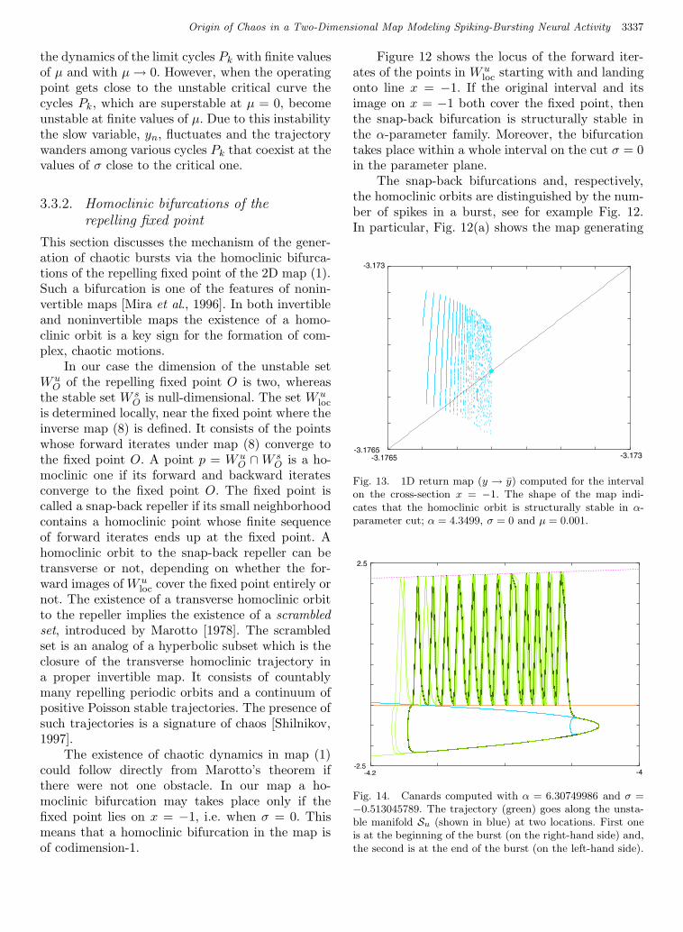
Figure 12 shows the locus of the forward iter-ates of the points in W u

loc starting with and landingonto line x = −1. If the original interval and itsimage on x = −1 both cover the fixed point, thenthe snap-back bifurcation is structurally stable inthe α-parameter family. Moreover, the bifurcationtakes place within a whole interval on the cut σ = 0in the parameter plane.

The snap-back bifurcations and, respectively,the homoclinic orbits are distinguished by the num-ber of spikes in a burst, see for example Fig. 12.In particular, Fig. 12(a) shows the map generating

Fig. 13. 1D return map (y → y) computed for the intervalon the cross-section x = −1. The shape of the map indi-cates that the homoclinic orbit is structurally stable in α-parameter cut; α = 4.3499, σ = 0 and µ = 0.001.

Fig. 14. Canards computed with α = 6.30749986 and σ =−0.513045789. The trajectory (green) goes along the unsta-ble manifold Su (shown in blue) at two locations. First oneis at the beginning of the burst (on the right-hand side) and,the second is at the end of the burst (on the left-hand side).

December 3, 2003 10:25 00852


chaotic sequences of the single and the double-pulsebursts.

Another computer assisted way of proving thechaotic dynamics in the map near the snap-backrepeller relies on the analysis of a one-dimensionalreturn map of a segment on x = −1. This map isshown in Fig. 13 at α = 4.345. The interval un-der consideration is of size ∼ 10−5 whose right endpoint is the snap-back repeller. One can see that themap at the indicated parameter values is expansion. The points of intersections of the graph of the mapand the bisectrix correspond to the unstable peri-odic orbits of distinct periods. Moreover, since thefixed point is in the range of the map whose graphhas a foliated structure, this suggests the existenceof infinitely many homoclinic orbits accumulatingto the primary one. The last ones and the periodicpoints form a skeleton of a chaotic set which can bean attractor of the map generating the bursts withirregular numbers of spikes.

Another, yet similar, way of waveform transfor-mations is illustrated in Fig. 14 far from the homo-clinic bifurcation. As above, the core of the mecha-nism is the interplay between the unstable manifoldSu and the locus of the attractor. Recall that the di-rection of the jump — up or down of the phase pointlanding onto the line x = −1 is determined whetherits coordinates are above or below Su respectively.However, it may happen that the point passes closeby the intersection point of Su and x = −1. Thenit results in some successive iterates of the phasepoint running closely along Su until an accumula-tive sharp jump up or down. It is evident that theduration and the length of such canardic phase de-pends on how close the phase point was picked upor turns out intermediately to be next to Su.

4. Conclusion

Our bifurcation analysis reveals the origin of chaoticbehavior of a simple two-dimensional discrete-time model of spiking-bursting neural activity. Themodel consists of fast and slow subsystems coupledto each other. The individual dynamics of the fastsubsystem is characterized by existence of bistableregime, where a superstable limit cycle, correspond-ing to the spike generation, and a stable fixed point,corresponding to the silence, coexist. When thissubsystem is coupled with the slow subsystem thathas neutral individual stability the whole systembecomes capable of generating chaotic spiking andspiking-bursting activity.

We have shown that the instability of trajec-tories needed for onset of chaos generation occursdue to the formation of canard solutions or due tomotions near a snap-back repeller. The canard so-lutions are quite typical near the excitation thresh-old and the transition between continuous spikingand spiking-bursting behavior. The dynamics nearsnap-back repeller can occur in the spiking-burstingregime.

The instability itself is not sufficient to guaran-tee the chaotic behavior. A very important compo-nent of chaos in this map is the time discretization.Sharp changes of the period of spiking in ourdiscrete-time model provides mixing which is anecessary element in the formation of a chaoticset. Although the discretization of time is not anattribute of complex dynamics of biological neu-rons this discrete-time model captures the onsetof chaotic spiking-bursting behavior in real neu-rons quite well. Chaotic component in the modelbehavior caused by the discrete-timing can betreated here as the influence of complex high-dimensional dynamics of ionic currents and/or asa stochastic component of ionic channels whichbring irregularity to the spiking-bursting neuralactivity.

The canard transitions (safe and dangerous) inthis and similar maps that we have analyzed so fargive rise to a number of curious problems related tothe general theory of continuous and discrete Frenchducks as well as the relative numerical species. Oneof these is whether the stable and unstable criti-cal canard manifolds may cross in a way that sta-ble and unstable separatrices of a saddle point in a2D diffeomorphism do, and if it is so, what size of

the wriggles is, i.e. ∼ e−1

µ or the crossings may be

super-exponentially small ∼ e−

1

e−

1µ as conjectured

by [Gelfreich & Turaev, 2002]. A comprehensive an-swer is to engage the extremely precise computa-tions that are beyond the scope of the given study.Nevertheless, all our persistent attempts to detectthe crossing numerically using double precision havefailed. Another related issue is a tremendous sen-sibility of the orbits of the map near the canardthreshold where infinitesimal (in terms of computerprecision, i.e. 1012−13) changes in parameter val-ues imply signification qualitative and quantitativealterations in the behavior of the supposedly triv-ial solutions of the slow–fast maps, see Fig. 15. So,this intriguing problem is yet to open and to beunderstood.

December 3, 2003 10:25 00852


-3.09-3.07

-0.6

-1.5

Fig. 15. Disintegration of the unstable invariant curve Lu

into a nontrivial set (red dots) at α = 4.1, µ = 0.001 andσ = −0.0261131991686799. The attraction basing of “for-mer” Lu in the backward time is shown in yellow. The visualfractal thickness of the invariant curve (red) suggest a conjec-ture that the breakdown of the curve is accompanied by theformation of the heteroclinic wiggles (crossing) of the stableand unstable manifolds Ss and Su. Courtesy of C. Mira.

Acknowledgments

We would like to thank Dima Turaev and Chris-tian Mira for useful discussions, especially, aboutissues related to the fine structure of the canardsin the dynamics of maps. N. Rulkov was supportedin part by U.S. Department of Energy (grant DE-FG03-95ER14516).

References

Abarbanel, H. D. I., Rabinovich, M. I., Selverston,A., Bazhenov, M. V., Huerta, R., Sushchik, M. &Rubchinskii, L. [1996] “Synchronization in neuralnetworks,” Physics-Uspekhi 39, 337–362.

Arnold, V. I., Afrajmovich, V. S., Ilyashenko, Yu. S. &Shilnikov, L. P. [1994] “Bifurcation theory,” Dynami-

cal Systems, Encyclopaedia of Mathematical SciencesV (Springer-Verlag).

Belykh, V. N., Belykh, I. V., Colding-Joregensen, M. &Mosekilde, E. [2000] “Homoclinic bifurcations lead-ing to the emergence of bursting oscillations in cellmodel,” Eur. Phys. J. E3, 205–219.

Buchholtz, F., Golowash, J., Epstain, I. R. & Marder,E. [1992] “Mathematical-model of an identified stom-atogastric ganglion neuron,” J. Neurophysiol. 67,332–340.

Chay, T. R. [1985] “Chaos in a three-variable model ofan excitable cell,” Physica D16, 233–242.

Chay, T. R. [1990] “Electrical bursting and intracellu-lar Ca2+ oscillations in excitable cell models,” Biol.

Cybern. 63, 15–23.Chay, T. R., Fan, Y. S. & Lee, Y. S. [1995] “Bursting,

spiking, chaos, fractals, and universality in biologicalrhythms,” Int. J. Bifurcation and Chaos 5, 595–635.

Diener, M. [1981] “Canards et bifurcations,” in Math-

ematical Tools and Models for Control, Systems

Analysis and Signal Processing, Vol. 3, CNRS(Toulouse/Paris), pp. 289–313.

Eckhaus, W. [1983] A Standard Chase on French Ducks,Lecture Notes in Mathematics, Vol. 985, pp. 449–494.

Fenichel, N. [1979] “Geometric singular perturbationtheory,” J. Diff. Eq. 31, 53–98.

Gelfreich, V. & Turaev. D. [2002] verbal communication.Golomb, D., Guckenheimer, J. & Gueron, S. [1993] “Re-

duction of a channel-based model for a stomatogastricganglion LP neuron,” Biol. Cybern. 69, 129–137.

Guckenheimer, J., Hoffman, K. & Weckesserand, W.[2000] “Numerical computations of canards,” Int. J.

Bifurcation and Chaos 2, 2669–2689.Hindmarsh, J. L. & Rose, R. M. [1984] “A model of neu-

ronal bursting using 3 coupled 1st order differential-equations,” Proc. R. Soc. London B221(1222),87–102.

Hodgkin, A. L. & Huxley, A. F. [1952] “A quantitativedescription of membrane current and its applicationto conduction and excitation in nerve,” J. Physiol.

117, 500–544.Izhikevich, E. M. [2000] “Neural excitability, spiking

and bursting,” Int. J. Bifurcation and Chaos 10,1171–1266.

Marotto, J.R. [1978] “Snap-back repeller implies chaosin Rn,” J. Math. Anal. Appl. 63, 199–223.

Mira, C., Gardini, L., Barugola, A. & Cathala, J.-C.[1996] Chaotic Dynamics in Two-Dimenional Nonin-

vertable Maps (World Scientific, Singapore).Rinzel, J. [1985] “Bursting oscillations in an excitable

membrane model,” Ordinary and Partial Differen-

tial Equations, eds. Sleeman, B. D. & Jarvis, R. J.,Lecture Notes in Mathematics, Vol. 1151 (Springer,NY), pp. 304–316.

Rinzel, J. [1987] “A formal classification of burstingmechanisms in excitable systems,” in Mathematical

Topics in Population Biology, Morphogenesis, and

Neurosciences, eds. Teramoto, E. & Yamaguti, M.,Lecture Notes in Biomathematics, Vol. 71 (Springer,NY), pp. 267–281.

Rulkov, N. F. [2002] “Modeling of spiking-bursting neu-ral behavior using two-dimensional map,” Phys. Rev.

E65, 041922.Shilnikov, L. P. [1997] “Mathematical problems of non-

linear dynamics: A tutorial,” Int. J. Bifurcation and

Chaos 7, 1953–2003.

December 3, 2003 10:25 00852


Shilnikov, L. P., Shilnikov, A. L., Turaev, D. V. &Chua, L. O. [2001] Methods of Qualitative Theory

for Nonlinear Dynamics, Part II (World Scientific,Singapore).

Wang, X.-J. [1993] “Genesis of bursting oscillations inthe Hindmarch–Rose model and homoclinicity to achaotic saddle,” Physica D62, 263–274.

AppendixThe First Lyapunov Value L1

Here we present the calculations of the firstLyapunov value at the fixed point at the Andronov–Hopf bifurcation. The consideration is reduced tothe stability analysis of the critical fixed point ofthe local map:

x =α

1 − x+ y , (A.1a)

y = y − µ(x+ 1 − σ) . (A.1b)

Let us translate the fixed point to the origin byapplying the transformation

(

x

y

)

7→

x+ σ − 1

y + σ − 1 − α

2 − σ

.

Next we express the right-hand side of (A.1a) asthe Taylor polynomial; only first three terms willbe needed:

x = y +α

(2 − σ)2x+

α

(2 − σ)3x2

+α

(2 − σ)4x3 +O(x4) ,

y = y − µx .

(A.2)

Applying the coordinate transformation(

x

y

)

7→(

0 1

sinψ −1 cosψ + µ

)(

ξ

η

)

makes the linear part of (A.2) a rotation throughthe angle ψ:(

ξ

η

)

=

(

cosψ − sinψ,

sinψ cosψ,

)(

ξ

η

)

+

0α

(2 − σ)3η2 +

α

(2 − σ)4η3 +O(η4)

.

Having introduced z = ξ + iη, the map recasts inthe complex form

z = zeiψ + i

(

−α(z − z∗)2

4(2 − σ)3+ i

α(z − z∗)3

8(2 − σ)4

)

+O(|z|4) ,

where z∗ is the z-conjugate. As follows from[Shilnikov et al., 2001], the quadratic terms

z = zeiψ +c202z2 + c11zz

∗ +c022z∗2 +O(|z|3)

with

c20 = − iα

2(2 − σ)3, c11 =

iα

2(2 − σ)3,

c02 = − iα

2(2 − σ)3,

(A.3)

are eliminated by the normalizing transformation

z 7→z− c20e2iψ−eiψ z

2− c111 − eiψ

zz∗− c02e−2iψ−eiψ z

∗2.

The resulting normal form finally assumes thecanonical form:

z = eiψ + L1z2z∗ +O(|z|3) ,

where O(|z|3) denotes the remaining cubic andhigher order terms. The expression for the firstLyapunov value reads as follows:

L1 = −Re

[

e−iψc212

]

+ Re(1 − 2eiψ)e−2iψc20c11

2(1 − eiψ)

+|c11|2

2+

|c02|24

. (A.4)

Plugging (A.3) into (A.4) yields

L1 =(2 − µ)(1 − µ)(4 − 2µ+ µ2)

16(2 − σ)2. (A.5)

One can see L1 > 0 when µ is small.Note that as follows from [Arnold et al., 1994]

the sign of L1 might be estimated as ∂3x/∂x3 from(A.2) at σ = 0 and α = 4. This is in agreement with(A.5).

origin of chaos in a two-dimensional map...

Documents