ordinary diﬀerential equations - indian institute of ... diﬀerential equations swaroop nandan...

Ordinary Differential Equations

Swaroop Nandan Bora

[email protected]

Department of Mathematics

Indian Institute of Technology Guwahati

Guwahati-781039

Teachers’ Training Camp, IITG, July 4, 2016

Swaroop Nandan Bora [email protected] (Department of MathematicsIndian Institute of Technology GuwahatiGuwahati-781039 )IITG, Differential EquationsTeachers’ Training Camp, IITG, July 4, 2016

/ 19


/ 19

A first-order differential equation is an equation

dy

dx= f(x, y)

in which

f(x, y) is a function of two variables defined on a region in the xy-plane.

A solution of the given equation is a differentiable function defined

on an interval I of x-values (perhaps infinite) such that

d

dxy(x) = f(x, y(x))

on that interval.

The general solution to a first-order differential equation is a solution that contains all

possible solutions.


/ 19

The general solution always contains an arbitrary constant

but having this property doesnt mean a solution is the general solution.

Establishing that a solution is the general solution may require deeper results

from the theory of differential equations.


/ 19

We often need a particular rather than the general solution to a first-order

differential equation

dy

dx= f(x, y).

The particular solution satisfying the initial condition y(x0) = y0 is the solution

whose value is y0 when x = x0.

Thus the graph of the particular solution passes through the point (x0, y0) in the

xy-plane.

A first-order initial-value problem is a differential equation

dy

dx= f(x, y) whose solution must satisfy an initial condition y(x0) = y0.


/ 19

Every differential equation need not have a solution.

Even if solution exists, that may not be unique.

Picard’s theorem:

Suppose f(x, y) and∂f

∂yare continuous on the interior of a rectangle R, and that

(x0, y0) is an interior point of R, then the IVP

dy

dx= f(x, y), y(x0) = y0

has unique solution y = y(x) for x in some open interval containing x0.


/ 19

Applications

Orthogonal trajectories

Let F (x, y, c) = 0 be a given one-parameter family of curves in the xy-plane.

A curve that intersects the curves of the above family at right angles

is called an orthogonal trajectory of the given family.

Main point:

Suppose that the differential equation of above family can be obtained as

dy

dx= f(x, y).

Then the orthogonal trajectory must have a slope

−1/(f(x, y)).


/ 19

Examples

Example 1

Given a family of circles: x2 + y2 = a2.

Its differential equation is obtained as

dy

dx= −

x

y

Differential equation of the orthogonal trajectory

dy

dx=

y

x

Giving the orthogonal trajectory as

y = kx,

all are straight lines passing through the origin.


/ 19

Example 2

Given a family of parabolas:

y = cx2.

The differential equation is

dy

dx=

2y

x.

The differential equation of the orthogonal trajectory

dy

dx= −

x

2y.

which gives us

x2 + 2y2 = k2.


/ 19

Problems in Mechanics

Newton’s 2nd law of motion

mdv

dt= F.

Example

A body of weight 8 pounds falls from rest toward the earth from a great height. As it

falls, air resistance acts upon it which is numerically equal to 2v, where v is the

velocity in feet per second. To find the velocity and distance covered in time t.

Differential equation is

mdv

dt= F1 + F2.

g = 32, w = 8, m = 8/32 = 1/4

1

4

dv

dt= 8− 2v.

Since the body falls from rest,

initial condition is v(0) = 0.


/ 19

Example 2

Solving it and using the initial condition

v = 4(1 − e−8t)

For finding the distance, the differential equation is

dx

dt= 4(1 − e−8t)

Solving and using the initial condition

x = 4(t+1

8e−8t

−

1

8)


/ 19

Interpretation of results

The solution for v tells us that

as t → ∞, then v reaches the limiting velocity 4 (ft/sec).

Again the solution for x tells us that

as t → ∞, then x also → ∞.

Does this imply that the body will pierce through the earth and continue

forever??

Of course not.

Because

when the body reaches the earth’s surface, the above differential equations no longer

apply.


/ 19

Rate of growth and decay

Example

The rate at which a radioactive nuclei decay is proportional to the number of such

nuclei that are present in a given sample. Half of the original number of radioactive

nuclei have undergone disintegration in a period of 1500 years.

What percentage of the original radioactive nuclei will remain after 4500 years?

Formulation:

Let x be the amount of radioactive nuclei present after t years.

The differential equation is

dx

dt= kx.

The initial condition is, given x0 is the amount present initially,

x(0) = x0.

But according to the given condition

x(1500) =1

2x0.


/ 19

Rate of growth and decay

Solution:

The solution is:

x = ce−kt.

By using the condition of half-life

e−k = (1

2)1/1500.

Therefore the solution is

x = x0[(1

2)1/1500]t.

For (i)

x = x0(1

2)3 =

1

8x0.

that is, 12.5 percent of original number remain after 4500 years.


/ 19

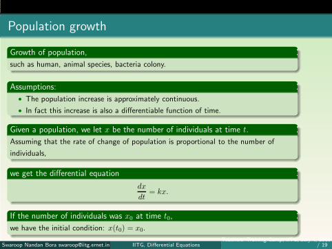
Population growth

Growth of population,

such as human, animal species, bacteria colony.

Assumptions:

• The population increase is approximately continuous.

• In fact this increase is also a differentiable function of time.

Given a population, we let x be the number of individuals at time t.

Assuming that the rate of change of population is proportional to the number of

individuals,

we get the differential equation

dx

dt= kx.

If the number of individuals was x0 at time t0,

we have the initial condition: x(t0) = x0.


/ 19

Population growth

The solution is given by

x(t) = x0ek(t− t0).

The population governed by this model (increasing exponentially with time) is

known as

Malthusian law.

But more realistically in many cases

the number of individuals x at time t is described by a differential equation

dx

dt= kx− λx2.

The additional term −λx2

is the result of some cause that tends to limit the ultimate growth of the population.


/ 19

Mixture problem

A substance S is allowed to flow into a certain mixture in a container at a certain

rate. The mixture is kept uniform by stirring.

Further, in one such situation, this uniform mixture simultaneously flows out of the

container at another (generally different rate.

Letting x denote the amount of S present at time t, the derivative dx/dt denotes the

rate of change of x with respect to t.

If IN denotes the rate at which S enters the mixture and OUT denotes the rate at

which it leaves,

Then we have the differential equation

dx

dt= IN −OUT.


/ 19

Example

A tank initially contains 50 gallons of pure water. Starting at time t = 0, a brine

containing 2 lb of dissolved salt per gallon flows into the tank at the rate of 3 gal/min.

The mixture is kept uniform by stirring and the well-mixed mixture simultaneously

flows out of the tank at the same rate. To find the amount of salt at time t.

Formulation:

dx

dt= IN −OUT.

IN= (2 lb/gal)(3 gal/min)= 6 lb/min

OUT =( x

50lb/gal

)

(3gal/min) =3x

50lb/min.

The initial value problem is

dx

dt= 6−

3x

50, x(0) = 0.


/ 19

Mixture problem

Solution

x = 100 + ce−3t/50.

Using the initial condition

x = 100(1 − e−3t/50).

How much salt is present at the end of 25 minutes?

x(25) = 100(1 − e−1.5) ≡ 78lb.

What happens when t → ∞?


/ 19

ordinary diﬀerential equations - indian institute of ... diﬀerential equations swaroop nandan...

Documents