Ordinal Notations and Well-Orderings in

Bounded Arithmetic

Arnold Beckmann1,3 Samuel R. Buss1,4 Chris Pollett2

June 25, 2002

1 Introduction

Ordinal notations and provability of well-foundedness have been a central toolin the study of the consistency strength and computational strength of formaltheories of arithmetic. This development began with Gentzen’s consistencyproof for Peano arithmetic based on the well-foundedness of ordinal notationsup to ε0. Since the work of Gentzen, ordinal notations and provable well-foundedness have been studied extensively for many other formal systems, somestronger and some weaker than Peano arithmetic. In the present paper, weinvestigate the provability and non-provability of well-foundedness of ordinalnotations in very weak theories of bounded arithmetic, notably the theoriesSi

2 and T i2 with 1 ≤ i ≤ 2. We prove several results about the provability of

well-foundedness for ordinal notations; our main results state that for the usualordinal notations for ordinals below ε0 and Γ0, the theories T 1

2 and S22 can prove

the ordinal Σb1-minimization principle over a bounded domain. PLS is the class

of functions computed by a polynomial local search to minimize a cost function.It is a corollary of our theorems that the cost function can be allowed to takeon ordinal values below Γ0, without increasing the class PLS.

The historical development of ordinal notations and formal theories of arith-metic is far too extensive for us to survey here. We shall include the basicdefinitions for ordinal notations of ordinals below ε0 and Γ0, and the reader canrefer to Feferman [6, 7] or the textbooks of Schutte [12] or Pohlers [11] for moredetails.

Theories of bounded arithmetic are fragments of Peano arithmetic whichhave induction strongly restricted, firstly to allow induction only on certain

1Dept. of Mathematics, Univ. of California, San Diego, La Jolla, CA 92093-0112.2Computer Science Dept., San Jose State Univ., One Washington Square, San Jose, CA

95192. Work performed while at the Dept. of Mathematics, UCLA.3Supported by the Deutschen Akademie der Naturforscher Leopoldina grant #BMBF-

LPD 9801-7 with funds from the Bundesministeriums fur Bildung, Wissenschaft, Forschungund Technologie.

4Supported in part by NSF grants DMS-0100589 and DMS-9803515 and by a cooperativeresearch grant INT-9600919/ME-103 of the NSF (USA) and the MSMT (Czech Republic).

1

types of bounded formulas, and secondly, in the case of the theories Si2, to allow

only length induction instead of the usual successor induction. In order to getmeaningful results, we need to work with theories such as S1

2 , T 12 , S2

2 and T 22 as

introduced by the second author in [3]. We presume the reader is familiar withthese theories of bounded arithmetic: the necessary background can be foundin [3, 4, 8, 10].

Ordinal notations have been extensively used in the study of strong theo-ries, ranging from primitive recursive arithmetic, to Peano arithmetic and tofragments of second-order arithmetic; however, there has been little prior workrelating ordinals to proof systems as weak as fragments of bounded arithmetic.This is due, in part, to the fact that the fragments of bounded arithmetic havecomputational complexity related to (near) feasible classes such as polynomialtime and the various levels of the polynomial time hierarchy. There are no goodmechanisms available to combine such low-level complexity with ordinal recur-sion, and thus traditional results on ordinal notations have not transferred tothe setting of bounded arithmetic. Sommer [14] investigated the formalizabilityof abstract ordinal notations in full bounded arithmetic, I∆0, and showed thatI∆0 can represent ordinals up to Γ0 with the ordinal operations of addition andthe Veblen ϕ function. Beckmann introduced dynamic ordinals in fragmentsof the bounded arithmetic as a tool to analyze predicative bounded arithmeticand to obtain relativized separation results for bounded arithmetic theories [1].His dynamic ordinals are based on exponential notations for integers, which aresimilar to the Cantor normal form representation of ordinals less than ε0.

It is known (c.f. [13]) that if one formalizes transfinite induction on ordinalsin the usual way, then induction on ordinals below ωω (or even induction on justω2) is sufficient to give the full strength of primitive recursive arithmetic. Thus,in order to get meaningful ordinal well-foundedness results for fragments ofbounded arithmetic it is necessary to limit the strength of the well-foundednessprinciples. We shall do this by restricting to a finite domain as follows. LetT be a first-order theory of bounded arithmetic and ≺ be a binary relationwhich T -provably defines a total ordering on a domain D ⊆ N. In practice, wewill require that ≺ and D are polynomial time recognizable predicates, definedby ∆b

1-formulas. We say that ≺ is well-founded on bounded domains providedthat whenever A(x) is a predicate and there is a d ∈ D such that d ≤ t andA(d), then there is a ≺-least element d ∈ D satisfying both d ≤ t and A(d). Insymbols, we write this principle as the formula WFA(t):

(∃d ≤ t)(d ∈ D ∧ A(d)) →(∃d ≤ t)[d ∈ D ∧ A(d) ∧ (∀d′ ≤ t)(d′ ∈ D ∧ A(d′) → d′ ⊀ d)].

(1)

It is of course a triviality that every total order is well-founded on boundeddomains, since bounded domains are finite sets. However, if a theory T canprove (1) for all Σb

1-formulas A(x) then we say that ≺ is provably well-foundedon bounded domains in T . 5 We let WF≺ denote the axiom scheme containingthe formulas WFA for all Σb

1-formulas A.5One could consider more general concepts, e.g., Σb

i -well-foundedness on bounded domains

2

The use of the domain D in the above definition is merely a convenience;there would be no loss in generality in taking D = N. Indeed, the ordering ≺can always be extended to have domain all integers by making d ≺ x for alld ∈ D and x /∈ D. The reason for using the domain D is that we will considernatural orderings on ordinal notations for ordinals below ε0 and Γ0: it will beconvenient to take D to be the set of valid Godel numbers for ordinal notations.

Very recently (and independently of our own work), Sommer has announcedsharpened versions of the above-mentioned results from [13]. In our notation,what he has done is modify the quantifier (∀d′ ≤ t) of formula (1) by replacing twith a bound f(d) which depends on d (and remove the other uses of t). Weknow no direct connection of this to our well-ordering principles on boundeddomains.

The outline of the present paper is as follows. In the next section, we showfirst that T 2

2 is strong enough to prove the well-foundedness on bounded do-mains of any ∆b

1-defined total ordering. On the other hand, we show that ifthe ordering is defined with an oracle, then T 1

2 and S22 cannot prove the well-

foundedness on bounded domains of the ordering. Section 3 considers the usualCantor normal form representation of ordinals below ε0: First we show that thewell-foundedness of this system is not provable in S1

2 unless S12 = T 1

2 . Second,we prove that T 1

2 can prove the well-foundedness of these ordinals on boundeddomains, by giving an order-preserving embedding of the ordinals less than ε0restricted to a bounded number of operators into Nk for some integer k. Sec-tion 4 introduces the usual Veblen ϕ-function notation for ordinals less than Γ0.It is shown that S1

2 can ∆b1 define the ordering on ordinals below Γ0 by giving

straightforward polynomial time algorithms (this re-obtains, more concretely,some results of Sommer [14]). In addition, S1

2 can define the normal form onordinals below Γ0 and prove that normal forms exist and are unique. Afterthis, we reach the central results of the paper: we prove that T 1

2 and S22 can

prove the well-foundedness on bounded domains of usual ordinal notations forordinals below Γ0.

Section 5 is a short diversion discussing order-preserving embeddings of or-dinals into the set of lexicographically-ordered words over a finite alphabet.

Finally, in section 6, we discuss a corollary of our theorems for the classPolynomial Local Search, PLS, introduced by Johnson, Papadimitriou and Yan-nakakis [9]. Buss-Krajıcek [5] showed that the Σb

1-definable functions of T 12 are

precisely the (multivalued) functions which are definable as the composition ofa projection function and a PLS function. We define the classes (ε0,4)-PLSand (Γ0,4)-PLS by generalizing PLS to allow the cost function to take on or-dinal values less than ε0 or Γ0, respectively. It is a corollary of our theorems onthe provability of well-foundedness of ordinal notations in T 1

2 , that the classes(ε0,4)-PLS and (Γ0,4)-PLS are identical to the class PLS.

We thank R. Sommer for useful discussions and remarks, which lead to aconsiderable simplification of some of the proofs.

defined with A ranging over Σbi -formulas. However, we shall not consider these generalizations

in this paper.

3

2 General orderings

This section states a couple results about general orderings. By a “generalordering” we mean any order defined by a ∆b

1-formula; by comparison the resultsof sections 3 and 4 concern specific natural well-orderings based on ordinalnotations.

To formalize general well-orderings, it is best to introduce ≺ as new relationsymbol in the language. Let Total(≺) be the formula expressing the conditionthat ≺ is a total ordering, i.e., that ≺ is transitive and satisfies trichotomy. Thiscan be formalized by

(∀x)(∀y)(∀z)[(x 6≺ x) ∧ (x ≺ y ∨ x = y ∨ y ≺ x)∧ (x ≺ y ∧ y ≺ z → x ≺ z)]

Note that Total(≺) is a ∀∆b0(≺)-formula. Let T 2

2 (≺)+Total(≺) be the theory ofbounded arithmetic axiomatized by the BASIC axioms, the successor inductionaxioms (IND) for Σb

2(≺) formulas and the axiom Total(≺).

Theorem 1 The ordering ≺ is provably well-founded on bounded domains overT 2

2 (≺) + Total(≺).

Proof Fix A(x) ∈ Σb1 (or even, A ∈ Σb

1(≺)). Clearly, WFA(y) is a Σb2(≺)-

formula. Let T be the theory T 22 (≺) + Total(≺). Clearly, T ` WFA(0) be-

cause the trichotomy of ≺ is implied by the axiom Total(≺). Also, T provesWFA(y) → WFA(y+1). Thus, by Σb

2(≺)-IND, T ` (∀y)WFA(y), which is whatwe needed to prove. 2

For weaker theories, we have:

Theorem 2 The ordering ≺ is not provably well-founded on bounded domainsover S2

2(≺) + Total(≺). In fact, S22(≺) + Total(≺) does not prove (∀y)WFA(y)

even for the case where A(x) is the universally true formula x = x.

Theorem 2 holds for T 12 (≺) + Total(≺) as well, since T 1

2 ⊆ S22 .

Proof Our proof exploits a proof technique of Krajıcek [10, Thm. 11.2.5]. LetS be the theory S2

2(≺) + Total(≺). Let A(x) be the formula “x = x”. (In factany formula A(x) which is true for a superpolynomial density of x’s could beused.) If S proves (∀y)WFA(y), then S can also prove the assertion

(∀y)(∃x ≤ y)(∀z ≤ y)(x 4 z). (2)

Suppose for the sake of obtaining a contradiction, that S can prove (2). This is a∀Σb

2-formula; therefore, by the relativization of the ‘main theorem’ for S22 , there

is a p2(≺) = PNP (≺)-function f which, given an input y, produces a ≺-least x

below y [3]. The function f runs in polynomial time and uses an NP (≺)-oracle.6

6One might also let the computation of f query the predicate ≺, but this is not necessary,since these queries may be made indirectly through the NP (≺) oracle.

4

The NP (≺) oracle is a nondeterministic oracle Turing machine M(u), which oninput u returns True iff it has an accepting computation. The machine M isallowed to make queries of the form “v ≺ w?” to the oracle ≺. In addition,f is Σb

2-defined by S, and S can prove all the relevant properties of f and themachine M . In particular, S can prove ∀y∀z ≤ y(f(y) 4 z).

Since f(y) runs in polynomial time, say in time p(|y|), any query u to Mmade during the computation of f must have |u| ≤ p(|y|). M also is polynomialtime, so there is a polynomial q bounding the runtime of M . In particular, anyparticular computation path of M(u) can make at most q(|u|) queries “v ≺ w?”to the oracle.

To prove Theorem 2, it will suffice to construct an oracle ≺ for which f failsto correctly produce the ≺-least x ≤ y. To do this, choose y sufficiently large,and run the polynomial time algorithm for computing f(y). As we computef(y), we construct a series of linear orders ≺i, i = 0, 1, 2, 3, .... The order ≺i

will have domain Di and with Di ⊆ Di+1 and each ≺i will be the restrictionof ≺i+1 to the domain Di.

Initially, we set ≺0 to be the empty binary relation with domain D0 = ∅.When f(y) makes its (i + 1)-st query, u, to M , we define ≺i+1. To define≺i+1, first consider the case that there is some total, linear order ≺ extending≺i such that that M(u) accepts relative to ≺. Choose, arbitrarily, such a ≺and an accepting computation of M(u) relative to u. Then, let Di+1 equal Di

union the set of values v, w such that M(u) made a query “v ≺ w?” in thisaccepting computation. Let ≺i+1 equal ≺ restricted to the domain Di+1. Thissame computation path will cause M(u) to accept relative to any linear orderingcontaining ≺i+1. In this case, the computation of f(u) then continues with aTrue answer from the oracle. In the second case, there is no such ordering ≺: set≺i+1=≺i and Di+1 = Di. M(u) will not accept relative to any linear orderingextending ≺i+1. In this case, the computation of f(y) is continued with a Falseanswer from the oracle query.

Note that in either case, Di+1 has at most 2q(|u|) ≤ 2q(p(|y|)) new elementsover Di. At the end of the computation f outputs a value x. The computationmade k ≤ p(|y|) queries to M(u), so we obtain a linear order ≺k with domain Dk

of cardinality at most 2p(|y|)·q(p(|y|)). If ≺ is any total linear order with domainN which extends ≺k, then the computation of f relative to ≺ will will have thesame answers to its oracle queries and hence must output the same value x. Ify was sufficiently large, namely if y > 2p(|y|)q(p(|y|)) + 1, then we can extend≺k to an ordering ≺ such that there is some z ≤ y with z ≺ x: this is done bychoosing z ∈ [0, y] \ (Dk ∪ {x}) and letting z be the least element of ≺. Thiscontradicts the fact that f(y) was to produce the ≺-least element x ≤ y. 2

We do not know of any way to extend Theorem 2 to a non-oracle styleresult. For instance, does there exist a ∆b

1-definition of a binary predicate ≺such that S1

2 ` Total(≺) and such that the theory S12 + WF≺ includes all the

∀Σb2-consequences of T 2

2 ?

5

3 Ordinals below ε0

3.1 Ordinal notations for ε0

We use < and ≤ to denote the usual ordering on ordinals; i.e., < denotes the‘real’ semantic concept of ordinal orderings, and we will reserve the symbol ≺for syntactically defined orderings on Godel numbers of ordinals. We reservelowercase Greek letters to denote ordinals or Godel numbers of ordinals. Recallthe Cantor normal form for ordinals; i.e., every ordinal α > 0 can be writtenuniquely in the form

α = ωα1 + ωα2 + ωα3 + · · · + ωαk ,

where k ≥ 1 and α1 ≥ α2 ≥ α3 ≥ · · · ≥ αk. This is the basis for the well-knownrepresentation of ordinals less than ε0: namely, write an ordinal α < ε0 as aterm in Cantor normal form, recursively writing the exponents of ω in the sameform.

This gives a syntactic representation of ordinals less than ε0. We need toformalize this syntactic representation in the bounded arithmetic theory S1

2 , bydefining a set D which is the set of Godel numbers of (syntactic representationsof) ordinals less than ε0 and a binary formula ≺ which defines the ordinalordering on the Godel numbers. The formulas D and ≺ need to be ∆b

1-formulas,that is to say, polynomial time computable, and S1

2 needs to be able to provethat ≺ defines a total ordering on the domain D.

The syntactic representation in S12 is developed in two stages: first repre-

senting ordinals in non-normal form, and then showing that ordinals can beconverted to the normal form. Ordinals will first be represented in a ‘basicform’ and then to make our results more general, in a ‘compact form’. As anexample of the difference,

ωω0+ω0+ω0+ ωω0+ω0+ω0

is in basic form, and its compact form is ωω0·3 · 2.

Definition The set of basic forms for ordinals less than ε0 is the set of expres-sions inductively defined as follows:

1. 0 is a basic form.

2. If α is a basic form, then so is ωα. The expression ωα is called an ω-term.

3. If α and β are basic forms, and α is an ω-term and β 6= 0, then α + β is abasic form.

S12 can formalize the notion of basic form by using standard sequence coding

methods to define the Godel number of a basic form. We assume that someefficient method of sequence coding is used for Godel numbers so that the lengthof the Godel number of a basic form α is proportional to the number of symbolsin α.

6

It is immediate from the definition that every non-zero basic form α can bewritten uniquely in its additive expansion

α = α1 + α2 + · · · + αk,

where each αi is an ω-term. Note that S12 is able to prove the existence and

uniqueness of the additive expansion of a basic form. To put basic forms intoa normal form, we wish to further require that the ordinals α1, . . . , αk form anon-increasing sequence. To formalize this, we first need to define a syntacticorder, denoted ≺, on basic forms. Unfortunately, the definition of the ≺ iscomplicated by the fact that basic forms are not (yet) in normal form.

Definition Let α and β be basic forms. We inductively define α 4 β andα 64 β, letting α ≈ β mean that both α 4 β and β 4 α, and α ≺ β mean thatα 4 β and α 6≈ β. First if α = 0, then α 4 β. Also, if β = 0 and α 6= 0, thenα 64 β. Otherwise, let α1 + · · ·+αk and β1 + · · ·+β` be the additive expansionsof α and β. Then

a. If k = ` = 1, and α1 = ωα′and β1 = ωβ′

, then α 4 β is defined to hold ifand only if α′ 4 β′.

b. If α1 ≺ αi for some i > 1, then α 4 β if and only if α2 + . . . + αk 4 β.

c. If β1 ≺ βi for some i > 1, then α 4 β if and only if α 4 β2 + . . . + β`.

d. Otherwise, if none of a., b., or c. apply, then α 4 β iff either (1) α1 ≺ β1

or (2) α1 ≈ β1 and α2 + · · ·+ αk 4 β2 + · · ·+ β`. (If either k or ` are one,then the empty sum is interpreted as 0.)

It is easy to show that 4 is transitive and reflexive and satisfies dichotomy,i.e., for all basic forms α, β, γ,

α 4 α,

α 4 β ∨ β 4 α,

α 4 β ∧ β 4 γ → α 4 γ.

Likewise, ≺ is transitive and antisymmetric. The proofs of these facts useordinary integer induction and do not require transfinite induction. To make ≺a linear (non-partial) ordering, we need to mod out by the ≈ relation. The bestway to do this is identify normal forms for ordinal notations:

Definition The set of normal basic forms for ordinals less than ε0 is the set ofexpressions inductively defined as follows:

1. 0 is a normal basic form.

2. If α is a normal basic form, then so is ωα.

3′. Let α and β be normal basic forms, α be an ω-term and β be non-zerowith β′ the leading term in the additive expansion of β. If β′ 4 α, thenα + β is a normal basic form.

7

It is straightforward to see that S12 can ∆b

1-define the syntactic concepts of≺, 4 on basic forms, for instance using the techniques of [3, Ch. 7] for inductivedefinitions S1

2 , or of [1, 2] for defining exponential notations. Probably the moststraightforward way to define these concepts in S1

2 is to follow [1, 2] and use thefollowing polynomial time algorithm for determining if α 4 β: Given α and βas inputs, the algorithm first forms all pairs (α′, β′) with α′ a subterm of α andβ′ a subterm of β. Then, starting with shorter subterms, the algorithm decidesfor each such pair, whether α′ ≺ β′ or α′ ≈ β′ or β′ ≺ α′. This algorithmcan readily be formalized in S1

2 , and based on this algorithm, S12 can prove

properties of 4 such as transitivity, reflexivity and dichotomy.In addition, S1

2 can ∆b1-define the set of (Godel numbers of) normal basic

forms. Finally, S12 can prove that ≺ is a total ordering on the normal basic

forms, satisfying transitivity and trichotomy.

We now define the compact representations for ordinals less than ε0.

Definition The set of compact forms for ordinals less than ε0 is the set ofexpressions inductively defined as follows:

1. 0 is a compact form.

2. If α is a compact form and n ∈ N, n > 0, then ωα · n is a compact form.This is called an ω-term.

3. If α and β are compact forms, and α is an ω-term and β 6= 0, then α + βis a compact form.

The definition of ≺ for compact forms is complicated by the fact that wenot only need to discard additive terms that are ‘out of order’, but also need tocollect together the integer coefficients of the maximum additive term.

Definition Let α and β be compact forms. α 4 β and α 64 β are inductivelydefined as follows. As before, let α ≈ β mean that α 4 β and β 4 α, and α ≺ βmean that α 4 β and α 6≈ β. Also as before, if α = 0, then α 4 β; and if β = 0and α 6= 0, then α 64 β. Otherwise, let α1 + · · · + αk and β1 + · · · + β` be theadditive expansions of α and β, where αi = ωα′

i · ni and βi = ωβ′i · mi.

a. If k = ` = 1, then α 4 β is defined to hold if and only if either (1) α′1 ≺ β′

1

or (2) α′1 ≈ β′

1 and n1 ≤ m1.

b. If α′1 ≺ α′

i for some i > 1, then α 4 β if and only if α2 + . . . + αk 4 β.

c. If β′1 ≺ β′

i for some i > 1, then α 4 β if and only if α 4 β2 + . . . + β`.

d. Otherwise, if none of a., b. or c. apply, and if α′1 6≈ β′

1, then α 4 β iffα′

1 4 β′1.

e. If none of a., b., c., or d. apply, then let S = {i : α′i ≈ α′

1} and letT = {i : β′

i ≈ β′1}. Let nS =

∑i∈S ni and mT =

∑i∈T mi. If nS < mT ,

then α 4 β. If nS > mT , then α 64 β. If nS = mT , then α 4 β iff∑i>max(S) αi 4

∑i>max(T ) βi. If a summation is empty, it is interpreted

as zero.

8

To make ≺ a linear (non-partial) order, we restrict its domain to compactforms in normal form:

Definition The set of normal compact forms for ordinals less than ε0 is the setof expressions inductively defined as follows:

1. 0 is a normal compact form.

2. If α is a normal compact form and n > 0, then ωα ·n is a compact normalform.

3′. Let α and β be normal compact forms, α = ωα′ · n an ω-term and β benon-zero with ωβ′ · m the leading term in the additive expansion of β. Ifβ′ ≺ α′, then α + β is a normal compact form.

The predicates ≺ and 4 for compact forms can be seen to be polynomial timecomputable based on their inductive definitions, and the bounded arithmetictheory S1

2 can ∆b1-define the syntactic concepts of ≺, 4 on compact forms.

Similarly, S12 can ∆b

1-define the set of (Godel numbers of) normal compact formsand the set of normal compact forms is polynomial time recognizable. Finally,S1

2 can prove that ≺ is a total ordering on the normal compact forms, satisfyingtransitivity and trichotomy.

3.2 Provable well-foundedness on bounded domains

By Theorem 1, the well-foundedness of ≺ on bounded domains can be provedin T 2

2 . Theorem 4 will show that the well-foundedness on bounded domains of(compact form) ordinal notations below ε0 is provable in T 1

2 . Before statingand proving that result, we show that T 1

2 is the weakest fragment of boundedarithmetic which can prove the well-foundedness of ≺ on ε0.

Theorem 3 Let ≺ be the ordering on normal basic (or, compact) forms forordinals less than ε0. Over the base theory S1

2 , WF≺ implies Σb1-IND.

Therefore, S12 ` WF≺ implies S1

2 = T 12 . The latter condition is unlikely to hold,

since it implies that PNP [log] equals PNP [10, Thm. 10.3.1].

Proof Since normal basic forms are essentially a special case of normal compactforms, it suffices to prove the theorem for normal basic forms. The proof isquite simple, we just need to give a natural, polynomial time computable, orderpreserving, embedding of the integers into the normal basic forms. (The identitymapping n 7→ ω0 + ω0 + · · · + ω0 from the integers into the normal basic formscannot be used, since it has exponential growth rate and is not polynomialtime.) The mapping we use is as follows: let n ∈ N have binary representation(nk · · ·n1n0)2 with each ni ∈ {0, 1}. Let S = {i : ni = 1} and i0, i1, . . . ipenumerate S in decreasing order. Let αi be the basic form representing theordinal i, αi = ω0 + · · · + ω0 (i summands). We define ι(0) = 0 and, for n > 0,

ι(n) = ωαi0 + ωαi1 + · · ·ωαip .

9

The mapping ι is readily seen to be polynomial time and Σb1-definable in S1

2 .Furthermore, S1

2 can prove that ι is order-preserving, so that n < m iff ι(n) ≺ι(m). S1

2 can intensionally ∆b1-define the range of ι, and can Σb

1-define theinverse function ι−1.

To complete the proof, suppose that A(x) is a Σb1-formula: we must show

that S12 can prove the least number principle (MIN) for A. Let A∗(w) be the

formula w ∈ ran(ι) ∧A(ι−1(w)). Then the formula WFA∗ immediately impliesthe least number principle for A(x). 2

The proof really showed that over the base theory S12 , WF≺′ implies Σb

1-IND,where ≺′ is the restriction of ≺ to normal basic (or, compact) forms α ≺ ωω.

Theorem 4 Let ≺ be the ordering on normal basic (or, compact) forms. ThenT 1

2 ` WF≺.

It is sufficient to prove Theorem 4 for compact forms, since this subsumesthe case of basic forms. Before giving the proof, we give an order-preservingembedding from bounded domains of normal compact forms into fixed-lengthsequences of integers. A compact form may be thought of as a sequence ofsymbols from the alphabet A containing “ω”, “+”, the integers, and a special‘end of superscript’ symbol “↓”. The length of an ordinal notation is defined toequal the number of symbols in the expression.

Definition The length of a compact form α is denoted lh(α) and is defined by

• lh(0) = 1.

• The length of ωα · n equals lh(α) + 3.

• The length of α + β equals lh(α) + lh(β) + 1.

We assume that an efficient Godel encoding is used for compact forms; forinstance, based on encoding the sequences Seq(α) defined next. In particular,we require that 2 · lh(α) ≤ |α| holds provably for S1

2 .

Definition A is the set N ∪ {ω,+, ↓}, and A∗ is the set of finite sequencesover A. We use the infix operator a to denote sequence concatenation. Letα be a compact form. Then Seq(α) is the member of A∗ defined by:

• Seq(0) is 〈0〉. That is, the one element sequence containing the symbol 0.

• Seq(ωα · n) equals 〈ω〉aSeq(α)a〈↓, n〉.

• Seq(α + β) equals Seq(α)a〈+〉aSeq(β).

Note that the symbols ω and ↓ will appear in Seq(α) in pairs, and arebalanced like left and right parentheses. Also, for every α 6= 0, the two lastelements of of Seq(α) will be ↓, n for some integer n.

10

Definition The set A is linearly ordered by the convention that ↓< + < N < ωwith the integers inheriting their usual ordering. The induced lexicographicordering on A∗ is also denoted <.

Lemma 5 For any normal compact forms α and β, α ≺ β holds if and only ifSeq(α) < Seq(β).

Proof The proof is by induction on the lengths of α and β. For either α or βequal to zero, this fact is immediate. Otherwise, α will equal either ωα′ · n orωα′ · n + α′′ and likewise β will equal either ωβ′ · m or ωβ′ · m + β′′. If α′ ≺ β′,then the induction hypothesis implies that that Seq(α′) < Seq(β′) and thereforeSeq(α) < Seq(β). Similarly, if β′ ≺ α′, then Seq(β) < Seq(α).

So suppose α′ = β′. Then, if either n < m or m < n, then Seq(α) < Seq(β)or Seq(β) < Seq(α), respectively. Finally, if α′ = β′ and m = n, then we applythe induction hypotheses to the forms α′′ and β′′ if they are both present. 2

Let N∗ be the set of finite sequences over the integers under the usual lexi-cographic ordering. It is simple to give an order-preserving map from A∗ intoN∗. Namely, for w ∈ A∗, replace each element of the sequence w by a pair ofintegers: ω is replaced by 1, 0; an integer n is replaced by 0, n+2; the symbol +is replaced with 0, 1 and ↓ is replaced with 0, 0. The resulting sequence haslength twice as long as w. For α a compact form, we write Nat(α) to denote thesequence in N∗ which is the image of the sequence Seq(α). The previous lemmaimmediately implies that, for all normal compact forms, Nat(α) < Nat(β) ifand only if α ≺ β. We thus have:

Theorem 6 The mapping Nat is an order-preserving mapping from the set ofnormal compact forms into N∗. Furthermore, the length of the sequence Nat(α)is 2 · lh(α).

The theorem is proved from the discussion above. The bound on the lengthis immediate from the definition. Furthermore, the definition of the functionNat and the proof of the theorem can be carried out in S1

2 .We are now ready to prove Theorem 4. We argue informally in T 1

2 to proveWFA(y), for A a Σb

1-formula. Fix the value of y. Given an ordinal β ≤ y, everyinteger in the sequence Nat(β) is less than 2|y|. Thus, for any β ≤ y, we canencode Nat(β) by the single integer

nβ :=|y|∑i=0

2(|y|−i)|y|(Nat(β))i,

where the notation (−)i extracts the i-th entry of sequence, starting with i = 0for the first entry, and (Nat(β))i is to equal 0 when i is greater than or equalthe length of Nat(β). The mapping β 7→ nβ , from normal compact forms tointegers is still order-preserving, at least for ordinals β with |β| ≤ |y|. Let A∗(n)be the formula expressing

n = nβ for some β ≤ y such that A(β).

11

By Σb1-minimization (which is provable in T 1

2 ), there is a <-least n such thatA∗(n) holds. From n = nβ , there is a simple polynomial time procedure toobtain β. Therefore, T 1

2 proves that there is a ≺-least β ≤ y such that A(β)holds.

That completes the proof of Theorem 4. 2

The construction from the proof of Theorem 6 can also be applied directly tonormal basic form ordinals. For basic form ordinals, Seq gives an order preserv-ing map from the set of normal basic forms into finite sequences (words) overthe alphabet {↓,+, 0, 1, ω}, where the sequences are ordered lexicographically.(In fact, the 1’s may be omitted w.l.o.g.)

This is a theme we shall return to briefly in section 5.

4 Ordinals below Γ0

4.1 Ordinal notations for Γ0

Recall the binary Veblen function ϕ (cf. [6, 11]), which can be defined inthe following way: Letting ϕα(β) denote ϕαβ, then ϕ0 is the enumerationof the “additiven Hauptzahlen” (i.e. ϕ0(β) = ωβ), and, for α > 0, ϕα is theenumeration of the simultaneous fixed points of all ϕα′ with α′ < α, i.e. of{β : (∀α′ < α)ϕα′(β) = β}. Now Γα is the αth element in the enumeration of{γ : ϕγ0 = γ}. Then each ordinal α < Γ0 either is 0 or can be written uniquelyas

α = ϕα1β1 + . . . + ϕαkβk (3)

with αi, βi < ϕαiβi and ϕα1β1 ≥ . . . ≥ ϕαkβk. This is the basis for the well-known representation of ordinals less than Γ0: namely, write an ordinal α < Γ0

in the form (3), recursively writing the subterms in the same form. It givesa syntactic representation of ordinals less than Γ0. We need to formalize thissyntactic representation in the bounded arithmetic theory S1

2 , by defining a setD which is the set of Godel numbers of (syntactic representations of) ordinalsless than Γ0 and a binary formula ≺ which defines the ordinal ordering on theGodel numbers. The formulas D and ≺ need to be ∆b

1-formulas, that is to say,polynomial time computable, and S1

2 needs to be able to prove that ≺ definesa total ordering on the domain D.

The syntactic representation in S12 is developed in two stages: first repre-

senting ordinals in non-normal form, and then showing that ordinals can beconverted to the normal form.

Definition The set of basic forms for ordinals less than Γ0 is the set of expres-sions inductively defined as follows:

1. 0 is a basic form.

2. If α, β are basic forms, then so is (ϕαβ). We call the expression (ϕαβ) aϕ-term.

12

3. If α and β are basic forms, and α is a ϕ-term, then (α+β) is a basic form.

We henceforth omit parentheses and write just ϕαβ for (ϕαβ) whenever thereis no ambiguity.

As in the case of ε0, S12 can formalize the notion of basic form. It is immediate

from the definition that every basic form α can be written uniquely in its additiveexpansion

α = α1 + α2 + · · · + αk, (4)

where each αi for i < k is a ϕ-term, and αk either is zero or a ϕ-term. Notethat S1

2 is able to prove the existence and uniqueness of the additive expansionof a basic form. The fact that we allow (only) the last term in the additiveexpansion (4) to equal 0 will be a technical convenience later when we definedecompositions of normal forms. This does mean that we cannot directly com-bine two basic forms α and β using addition: instead we define α + β to be abasic term by defining: (a) 0 + β is the same as β and (b) for α 6= 0, α + β isdefined by writing α in its additive expansion (4), letting ` = k if αk 6= 0 and` = k − 1 if αk = 0, then letting α + β equal α1 + · · · + α` + β.

To put basic forms into a normal form, we wish to further require that anyadditive expansion (4) has the αi’s in non-increasing order, and that all ϕ-termsϕαβ satisfy α, β < ϕαβ. To formalize this, we first need to formalize a syntacticorder, denoted ≺, on basic forms.

Definition Let α and β be basic forms. We inductively define α 4 β andα 64 β, letting α ≈ β mean that both α 4 β and β 4 α, and α ≺ β mean thatα 4 β and α 6≈ β. First if α = 0, then α 4 β. Also, if β = 0 and α 6= 0, thenα 64 β. Otherwise, let α1 + · · ·+αk and β1 + · · ·+β` be the additive expansionsof α and β. Then

a. If k = ` = 1, α1 = ϕα′1α

′2 and β1 = ϕβ′

1β′2, then α 4 β is defined to hold

if and only if either (1) α′1 ≺ β′

1 and α′2 4 β1; or (2) α′

1 ≈ β′1 and α′

2 4 β′2;

or (3) β′1 ≺ α′

1 and α1 4 β′2 holds.

b. If α1 ≺ αi for some i > 1, then α 4 β if and only if α2 + . . . + αk 4 β.

c. If β1 ≺ βi for some i > 1, then α 4 β if and only if α 4 β2 + . . . + β`.

d. Otherwise, if none of a., b. or c. apply, then α 4 β iff either (1) α1 ≺ β1

or (2) α1 ≈ β1 and α2 + · · ·+ αk 4 β2 + · · ·+ β`. (If either k or ` are one,then the empty sum is interpreted as 0.)

The predicates ≺ and 4 for basic forms can be seen to be polynomial timecomputable based on their inductive definitions, and the bounded arithmetictheory S1

2 can ∆b1-define the syntactic concepts of ≺, 4 on basic forms. It is

easy to show that 4 is transitive and reflexive and satisfies dichotomy. Likewise,≺ is transitive and antisymmetric. The proofs of these facts use ordinary integerinduction and do not require transfinite induction and can be carried out in S1

2 .In fact, S1

2 can prove the following facts which we need for later work:

13

Proposition 7 (S12) For all basic forms α, β, γ,

1. α 4 β ∨ β 4 α. (Dichotomy)2. α 4 β ∧ β 4 γ → α 4 γ. (Transitivity)3. α ≺ β ∧ β ≺ γ → α ≺ γ. (Transitivity)4. α 4 α + β ∧ β 4 α + β.5. 0 ≺ ϕαβ.6. α ≺ β → ϕα(ϕβγ) ≈ ϕβγ.7. β ≺ γ ↔ ϕαβ ≺ ϕαγ.8. α ≺ β ↔ ϕα0 ≺ ϕβ0.9. β 4 ϕαβ.10. α ≺ ϕα0. Also, α ≺ ϕαβ.11. β 6≈ 0 → 1 4 β.12. α ≺ β → α + 1 4 β.13. ϕβγ 6= ϕ00 ∧ α ≺ ϕβγ → α + 1 ≺ ϕβγ.14. α ≺ β ↔ ϕα(γ + 1) ≺ ϕβ(γ + 1).

The expression “1” is an abbreviation for ϕ00. We shall not carry out theproofs of the assertions in Proposition 7. The proofs use induction and shouldbe carried out in the order the assertions are listed in the proposition.

The ordering ≺ is only a partial order on basic forms. To make ≺ a linear(non-partial) ordering, we need to mod out by the ≈ relation. The best wayto do this is identify normal forms for ordinal notations. Our definition of anormal form will be slightly nonstandard for technical reasons. The differenceis that additive expansions will always end with the term 0.

Definition The set of normal forms, also represented by NF, for ordinals lessthan Γ0 is the set of expressions inductively defined as follows:

1. 0 is a normal form.

2. Let α, β and γ be normal forms, α, β ≺ ϕαβ and γ′ be the leading termin the additive expansion of γ. If γ′ 4 ϕαβ, then ϕαβ + γ is a normalform.

The formulation of (2) has the effect that any ϕ-term is part of a summationthat ends with “+0”. This is a technical convenience which has the advantagethat any non-zero normal form β can be (uniquely) expressed in the form

β = ϕα1(ϕα2(. . . (ϕαb−1(ϕαb0 + γb) + γb−1) . . .) + γ2) + γ1

where of course some γi’s may be 0.S1

2 can ∆b1-define the set of (Godel numbers of) normal forms and the set

of normal forms is polynomial time recognizable. Further, S12 can prove that ≺

is a total ordering on the normal forms, satisfying transitivity and trichotomy,and that the following properties hold:

14

Proposition 8 (S12) Let “1” abbreviate the normal form ϕ00 + 0.

1. ∀α, β ∈ NF, if α ≈ β, then α = β.2. ≺ is a total order on normal forms (satisfies trichotomy and transitivity).3. ∀α, β ∈ NF, α + 1 and ϕα0 + 0 and ϕα(β + 1) + 0 are in NF.4. If α1 + · · · + αk ∈ NF, then α1 6≺ αi for all i.5. If α = β + γ ∈ NF and β ≺ δ and β and δ are ϕ-terms, then α ≺ δ.6. For all basic forms α, there is a β ∈ NF such that α ≈ β.7. If α ∈ NF and β is a proper subterm of α, then β ≺ α.

From items 1 and 6, every basic form corresponds to a unique normal form.The proof of the proposition is carried out similarly to the proof of the previousproposition. In order to prove 1, one first proves that

β ≺ ϕαβ ∧ δ ≺ ϕγδ ∧ ϕαβ ≈ ϕγδ → α ≈ γ ∧ β ≈ δ.

4.2 Decompositions

By Theorem 1 we know that the well-foundedness of ≺ on bounded domains canbe proved in T 2

2 . We will prove that the well-foundedness on bounded domainsof ordinal notations below Γ0 is provable in T 1

2 . We do this by describing ap1-algorithm that computes an order-preserving embedding of Γ0 into words,

i.e. finite sequences, over some finite alphabet together with the lexicographicordering. This embedding will map bounded domain ordinals to fixed lengthwords (i.e., the length will be bounded polynomially in the binary length of thebound to the ordinal domain). Using the same technique as in Section 3 wecan code fixed length words in an order-preserving fashion by natural numbers.This algorithm will be formalizable in S1

2 , and S12 will prove that it is order-

preserving. Hence the task of finding a ≺-minimal β satisfying a Σb1-formula

A(β) can be reduced to finding a <-minimal n satisfying some Σb1-formula A∗(n),

which can be solved in T 12 .

Our idea for computing the order-preserving embedding is to find certainmaximal elements in the decomposition of ordinals. E.g., assume β is a normalform. As mentioned above, β has the form

β = ϕα1(ϕα2(. . . (ϕαb0 + γb) . . .) + γ2) + γ1. (5)

Let α∗ be the maximal element of α1, . . . , αb with respect to ≺. Lemma 9 willshow that

ϕα∗0 4 β ≺ ϕ(α∗ + 1)0,

hence α∗ is the most important subterm β concerning ≺, which will come (lex-icographically) before others. We will recursively apply our algorithm to α∗,which is simpler, because the length of α∗ is smaller than that of β. Thenthe algorithm will make recursive calls to compute the other components of β,namely, the parts of β which are not in the subterm α∗.

In order to formalize this idea we start by defining the decomposition ofnon-zero normal forms in Γ0 as shown in equation (5).

15

Definition (Decomposition of β) Each normal form β ∈ Γ0 \ {0} can uniquelybe decomposed in the following way: Write β0 := β. Let βi 6= 0 be recursivelydefined, then we define αi+1, βi+1 and γi+1 by βi = ϕαi+1βi+1 + γi+1. Let b bethe index of the last βi, i.e. βb = 0. This expresses β as in equation (5). Thenwe define

α∗ := m1(β) := max≺{α1, . . . , αb}i∗ := min{i : αi = α∗}β∗ := m2(β) := βi∗

We call b; ~α; ~β;~γ;α∗;β∗; i∗ the decomposition of β. As β is non-zero and a normalform we immediately have b > 0, i∗ > 0 and that ~α, ~β, ~γ are all normal forms.

Example: Let β = ϕ2(ϕ10 + 1) + 0. The natural numbers occurring in thisterm stand for the normal forms representing that number, e.g. 1 abbreviatesthe normal form ϕ00 + 0. Then we decompose:

β0 = ϕ2(ϕ10 + 1) + 0α1 = 2 β1 = ϕ10 + 1 γ1 = 0α2 = 1 β2 = 0 γ2 = 1

Hence b = 2, α∗ = 2, i∗ = 1, β∗ = ϕ10 + 1.

In section 4.3, we present an algorithm for computing an order preservingembedding of ordinals below Γ0 into words over a finite alphabet. The intuitiveidea behind the embedding algorithm is that it first computes the componentsα∗ and β∗ of the decomposition of β, and recursively outputs the embedding ofα∗ and β∗. The algorithm then treats ρ = ϕα∗β∗ as a fixed subterm which hasbeen fully processed, and continues computing the embedding for the rest ofthe ordinal β recursively. This recursive computation above the fixed subterm ρworks with ordinals β which have decomposition containing a βi equal to ρ + γfor some γ. We call the set of ordinals β satisfying this condition a context. Toformally define contexts, we define classes Γ0[ρ] and Γ0[ρ] as follows:

Definition The variables α, β, γ, δ range over normal forms. The class Γ0[ρ] isinductively defined by:

1. Let γ 6= 0. If ϕα(ρ + γ) + δ is in normal form, then it is in Γ0[ρ].

2. Let β ∈ Γ0[ρ]. If ϕαβ + γ is in normal form, then it is in Γ0[ρ].

Γ0[ρ] contains Γ0[ρ] plus all normal form ordinals ρ + γ.

Before giving a detailed description of the embedding algorithm we estab-lish various properties of decompositions and contexts needed to prove the al-gorithm’s correctness.

16

Lemma 9 (S12) Let β ∈ NF \ {0} and α∗, β∗ be as above.

1. ϕα∗0 ¹ β ≺ ϕ(α∗ + 1)0.2. ϕα∗β∗ ¹ β ≺ ϕα∗(β∗ + 1).3. β ∈ Γ0[ϕα∗β∗]. In particular, if i∗ > 1, then γi∗ 6= 0.

Proof Since β < βi∗−1 < ϕα∗β∗ < ϕα∗0, we have the first inequalities in 1.and 2. To prove the second inequality in 1., we show βj ≺ ϕ(α∗ +1)0, for j ≤ b,by induction on j from b down to 0. In the base case, j = b, and βb = 0 so theassertion is obvious. For the induction step, let j < b. The induction hypothesisimplies

ϕαj+1βj+1 ≺ ϕαj+1(ϕ(α∗ + 1)0) ≈ ϕ(α∗ + 1)0

since αj+1 4 α∗ by the definition of α∗. Hence βj = ϕαj+1βj+1 + γj+1 ≺ϕ(α∗ + 1)0.

The second inequality in 2. is proved by a similar use of induction on j.In the base case, j = i∗ − 1; then βj = ϕα∗β∗ + γi∗ ≺ ϕα∗(β∗ + 1), sinceϕα∗β∗ ≺ ϕα∗(β∗ + 1). For the induction step, let j < i∗ − 1. By the inductionhypothesis we have

ϕαj+1βj+1 ≺ ϕαj+1(ϕα∗(β∗ + 1)) ≈ ϕα∗(β∗ + 1)

since αj+1 ≺ α∗ by the definition of α∗. Therefore βj = ϕαj+1βj+1 + γj+1 ≺ϕα∗(β∗ + 1).

The condition 3. is nearly obvious. The only thing to check is that γi∗ isnon-zero if β does not have the form ϕα∗β∗ + γi∗ . But in this case i∗ > 1,hence we have βi∗−2 = ϕαi∗−1(ϕα∗β∗ + γi∗) + γi∗−1. By definition of α∗ wehave αi∗−1 ≺ α∗. If γi∗ were zero, then we would have ϕαi∗−1(ϕα∗β∗ + γi∗) ≈ϕα∗β∗ + γi∗ contradicting βi∗−2 being a normal form. 2

We next generalize the notion of decomposition to decomposition of ordi-nals β in Γ0[ρ]. This is called decomposition above ρ and the main difference inthe process of forming the decomposition of β above ρ is that the process stopswhen the subterm ρ is reached. That is to say, the decomposition of β above ρwill be an expression of the form

β = ϕα1(ϕα2(. . . (ϕαb(ρ + γb+1) + γb) . . .) + γ2) + γ1. (6)

We will then define α∗,ρ to equal the ≺-maximal element of α1, . . . , αb and thiswill satisfy

ϕα∗,ρ(ρ + 1) 4 β ≺ ϕ(α∗,ρ + 1)(ρ + 1);

that is to say, α∗,ρ is the most important subterm of β above ρ (see Lemmas 10and 13).

Definition (Decomposition of β above ρ) Let ρ be a ϕ-term. Each β ∈ Γ0[ρ]can uniquely be decomposed in the following way. Let β0 := β. Inductivelydefine αi+1, βi+1 and γi+1 by βi = ϕαi+1βi+1 + γi+1. Let b be the index suchthat βb is of the form ρ + γb+1. This expresses β in the form of equation (6).

17

Then we define

α∗,ρ := mρ1(β) := max≺{α1, . . . , αb}

i∗,ρ := min{i : αi = α∗,ρ}β∗,ρ := mρ

2(β) := βi∗,ρ

We say that b; ~α; ~β;~γ;α∗,ρ;β∗,ρ; i∗,ρ is the decomposition of β above ρ. As β isa normal form in Γ0[ρ] we immediately have b > 0, i∗ > 0, γb+1 6= 0 and thatall ~α, ~β, ~γ are normal forms.

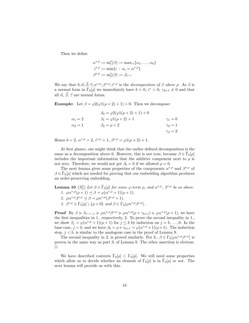
Example: Let β = ϕ2(ϕ1(ρ + 2) + 1) + 0. Then we decompose:

β0 = ϕ2(ϕ1(ρ + 2) + 1) + 0α1 = 2 β1 = ϕ1(ρ + 2) + 1 γ1 = 0α2 = 1 β2 = ρ + 2 γ2 = 1

γ3 = 2

Hence b = 2, α∗,ρ = 2, i∗,ρ = 1, β∗,ρ = ϕ1(ρ + 2) + 1.

At first glance, one might think that the earlier defined decomposition is thesame as a decomposition above 0. However, this is not true, because β ∈ Γ0[ρ]includes the important information that the additive component next to ρ isnot zero. Therefore, we would not get βb = 0 if we allowed ρ = 0.

The next lemma gives some properties of the components α∗,ρ and β∗,ρ ofβ ∈ Γ0[ρ] which are needed for proving that our embedding algorithm producesan order-preserving embedding.

Lemma 10 (S12) Let β ∈ Γ0[ρ] for some ϕ-term ρ, and α∗,ρ, β∗,ρ be as above.

1. ϕα∗,ρ(ρ + 1) ¹ β ≺ ϕ(α∗,ρ + 1)(ρ + 1).2. ϕα∗,ρβ∗,ρ ¹ β ≺ ϕα∗,ρ(β∗,ρ + 1).3. β∗,ρ ∈ Γ0[ρ] \ {ρ + 0} and β ∈ Γ0[ϕα∗,ρβ∗,ρ].

Proof By β < βi∗,ρ−1 < ϕα∗,ρβ∗,ρ < ϕα∗,ρ(ρ + γb+1) < ϕα∗,ρ(ρ + 1), we havethe first inequalities in 1., respectively, 2. To prove the second inequality in 1.,we show βj ≺ ϕ(α∗,ρ + 1)(ρ + 1) for j ≤ b by induction on j = b, . . . , 0. In thebase case, j = b, and we have βb = ρ+γb+1 ≺ ϕ(α∗,ρ +1)(ρ+1). The inductionstep, j < b, is similar to the analogous case in the proof of Lemma 9.

The second inequality in 2. is proved similarly. For 3., β ∈ Γ0[ϕα∗,ρβ∗,ρ] isproven in the same way as part 3. of Lemma 9. The other assertion is obvious.2

We have described contexts Γ0[ρ] ⊂ Γ0[ρ]. We will need some propertieswhich allow us to decide whether an element of Γ0[ρ] is in Γ0[ρ] or not. Thenext lemma will provide us with this.

18

Lemma 11 (S12) Let β, η ∈ Γ0[ρ] for some ϕ-term ρ.

1. β ∈ Γ0[ρ] ⇔ β < ϕ0(ρ + 1).2. β ∈ Γ0[ρ], β 4 η ⇒ η ∈ Γ0[ρ].

Proof 1.: Assume β ∈ Γ0[ρ]. Let b; ~α; ~β;~γ;α∗,ρ;β∗,ρ; i∗,ρ be the ρ-decomposi-tion of β. Then β < ϕαb(ρ + γb+1) < ϕ0(ρ + 1). To prove the converse, assumeβ ∈ Γ0[ρ] \ Γ0[ρ]. Then β = ρ + γ1 ≺ ϕ0(ρ + 1).

2.: Assume η 6∈ Γ0[ρ] and β ∈ Γ0[ρ]. Using 1. twice we obtain η ≺ ϕ0(ρ+1) 4β. 2

The next lemma states that the main components from decompositions re-spect the ordering of ordinals.

Lemma 12 (S12) Let β, η be normal forms with 0 ≺ β 4 η.

1. m1(β) 4 m1(η).2. m1(β) = m1(η) ⇒ m2(β) 4 m2(η).

Proof With β, η ∈ NF \ {0} we associate decompositions b; ~α; ~β;~γ;α∗;β∗; i∗

and n; ~ξ; ~η; ~µ; ξ∗; η∗; j∗, respectively. Then the lemma states:1. α∗ 4 ξ∗.2. α∗ = ξ∗ ⇒ β∗ 4 η∗.

We prove these by induction on b + n. Since β 4 η, we obtain ϕα1β1 4 ϕξ1η1.If ϕα1β1 ≈ ϕξ1η1, then ϕα1β1 = ϕξ1η1 as β, η ∈ NF, thus the assertions areobvious. Hence we assume ϕα1β1 ≺ ϕξ1η1. The proofs of 1. and 2. split intothree cases (I)-(III) depending on the reason that ϕα1β1 ≺ ϕξ1η1 holds.(I) Suppose α1 ≺ ξ1 and β1 ≺ ϕξ1η1.

1.: If i∗ = 1 we have α∗ = α1 ≺ ξ1 4 ξ∗. Otherwise i∗ > 1 and β1 6= 0,hence

α∗ = m1(β1)(∗)4 m1(ϕξ1η1) = ξ∗

using induction hypothesis at (∗).2.: Suppose α∗ = ξ∗. Then i∗ > 1, since otherwise α∗ = α1 ≺ ξ1 4 ξ∗ = α∗.

Therefore, β1 6= 0, α∗ = m1(β1), β∗ = m2(β1), hence m1(β1) = α∗ = ξ∗ =m1(ϕξ1η1), thus the induction hypothesis shows

β∗ = m2(β1) 4 m2(ϕξ1η1) = η∗.

(II) Suppose α1 = ξ1 and β1 ≺ η1.1.: If i∗ = 1 we have α∗ = α1 = ξ1 4 ξ∗. If i∗ > 1, then β1 6= 0 and hence

η1 6= 0. Hence by the induction hypothesis

α∗ = m1(β1)4 m1(η1) 4 ξ∗.

2.: Suppose α∗ = ξ∗. If i∗ = 1 we obtain ξ1 = α1 = α∗ = ξ∗, hence j∗ = 1,too. Thus

β∗ = β1 ≺ η1 = η∗.

19

Otherwise i∗, j∗ > 1, and again β1 6= 0 and η1 6= 0. By the induction hypothesiswe first obtain

α∗ = m1(β1) 4 m1(η1) = ξ∗ = α∗,

hence m1(β1) = m1(η1), and applying the induction hypothesis again yields

β∗ = m2(β1) 4 m2(η1) = η∗.

(III) Suppose α1 Â ξ1 and ϕα1β1 ≺ η1. So η1 6= 0.1.: By induction hypothesis we obtain

α∗ = m1(ϕα1β1) 4 m1(η1) 4 ξ∗.

2.: Suppose α∗ = ξ∗, then j∗ > 1, because otherwise ξ∗ = ξ1 ≺ α1 4 α∗ =ξ∗. Therefore, ξ∗ = m1(η1), η∗ = m2(η1), hence m1(ϕα1β1) = α∗ = ξ∗ =m1(η1). Thus the induction hypothesis shows

β∗ = m2(ϕα1β1) 4 m2(η1) = η∗.

2

Similar properties are needed for decompositions above ρ.

Lemma 13 (S12) Let β, η ∈ Γ0[ρ] with β 4 η.

1. mρ1(β) 4 mρ

1(η)2. mρ

1(β) = mρ1(η) ⇒ mρ

2(β) 4 mρ2(η).

Proof The proof of these assertions is simply a translation of the proof ofLemma 12 using the following Translation:

decomposition ; decomposition above ρ∗ ; ∗,ρ

· · · 6= 0 ; · · · ∈ Γ0[ρ]

The only additional thing we have to ensure is that the induction hypothesis isalways applicable; that is, that the terms under consideration are in Γ0[ρ]. 2

4.3 Algorithms

In this section, we formulate precisely the embedding algorithms and show thatthey are in p

1.

Definition The length of a basic form α is denoted lh(α) and is defined by

• lh(0) = 1.

• The length of ϕαβ equals lh(α) + lh(β) + 1.

• The length of α + β equals lh(α) + lh(β) + 1.

20

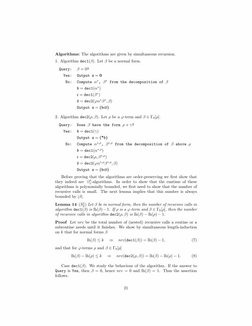
Algorithms: The algorithms are given by simultaneous recursion.

1. Algorithm dec1(β). Let β be a normal form.

Query: β = 0?

Yes: Output a = 0

No: Compute α∗, β∗ from the decomposition of β

b = dec1(α∗)

c = dec1(β∗)

d = dec2(ϕα∗β∗, β)

Output a = (bcd)

2. Algorithm dec2(ρ, β). Let ρ be a ϕ-term and β ∈ Γ0[ρ].

Query: Does β have the form ρ + γ?

Yes: b = dec1(γ)

Output a = (*b)

No: Compute α∗,ρ, β∗,ρ from the decomposition of β above ρ

b = dec1(α∗,ρ)

c = dec2(ρ, β∗,ρ)

d = dec2(ϕα∗,ρβ∗,ρ, β)

Output a = (bcd)

Before proving that the algorithms are order-preserving we first show thatthey indeed are p

1-algorithms. In order to show that the runtime of thesealgorithms is polynomially bounded, we first need to show that the number ofrecursive calls is small. The next lemma implies that this number is alwaysbounded by |β|.Lemma 14 (S1

2) Let β be in normal form, then the number of recursive calls inalgorithm dec1(β) is lh(β)−1. If ρ is a ϕ-term and β ∈ Γ0[ρ], then the numberof recursive calls in algorithm dec2(ρ, β) is lh(β) − lh(ρ) − 1.

Proof Let nrc be the total number of (nested) recursive calls a routine or asubroutine needs until it finishes. We show by simultaneous length-inductionon k that for normal forms β

lh(β) ≤ k ⇒ nrc(dec1(β)) = lh(β) − 1, (7)

and that for ϕ-terms ρ and β ∈ Γ0[ρ]

lh(β) − lh(ρ) ≤ k ⇒ nrc(dec2(ρ, β)) = lh(β) − lh(ρ) − 1. (8)

Case dec1(β). We study the behaviour of the algorithm. If the answer toQuery is Yes, then β = 0, hence nrc = 0 and lh(β) = 1. Thus the assertionfollows.

21

Otherwise the answer to Query is No. We compute

nrc = nrc(dec1(α∗)) + nrc(dec1(β∗)) + nrc(dec2(ϕα∗β∗, β)) + 3= (lh(α∗) − 1) + (lh(β∗) − 1) + (lh(β) − lh(ϕα∗β∗) − 1) + 3= lh(β) − 1.

Case dec2(ρ, β). If the answer to Query is Yes, then by the induction hy-pothesis we obtain nrc = nrc(dec1(γ)) + 1 = lh(γ) = lh(β) − lh(ρ) − 1 asβ = ρ + γ.

Otherwise the answer to Query is No. We compute

nrc = nrc(dec1(α∗,ρ)) + nrc(dec2(ρ, β∗,ρ)) + nrc(dec2(ϕα∗,ρβ∗,ρ, β)) + 3= (lh(α∗,ρ) − 1) + (lh(β∗,ρ) − lh(ρ) − 1) + (lh(β) − lh(ϕα∗,ρβ∗,ρ) − 1) + 3= lh(β) − lh(ρ) − 1.

As phrased above the induction is on a Πb2-formula. To formalize the proof

in S12 , we fix a particular β0 and prove the lemma holds for β0. For this, it is

enough to prove that (7) and (8) hold for all β and ρ which are subterms of β0.Quantifying over all subtems requires only a sharply bounded quantifier, so onlyΣb

1-PIND is needed.This finishes the proof of Lemma 14. 2

Using the previous lemma it is easy to obtain a polynomial runtime boundon the algorithms dec1 and dec2. Thus we have established:

Theorem 15 (S12) dec1 and dec2 are p

1-algorithms.

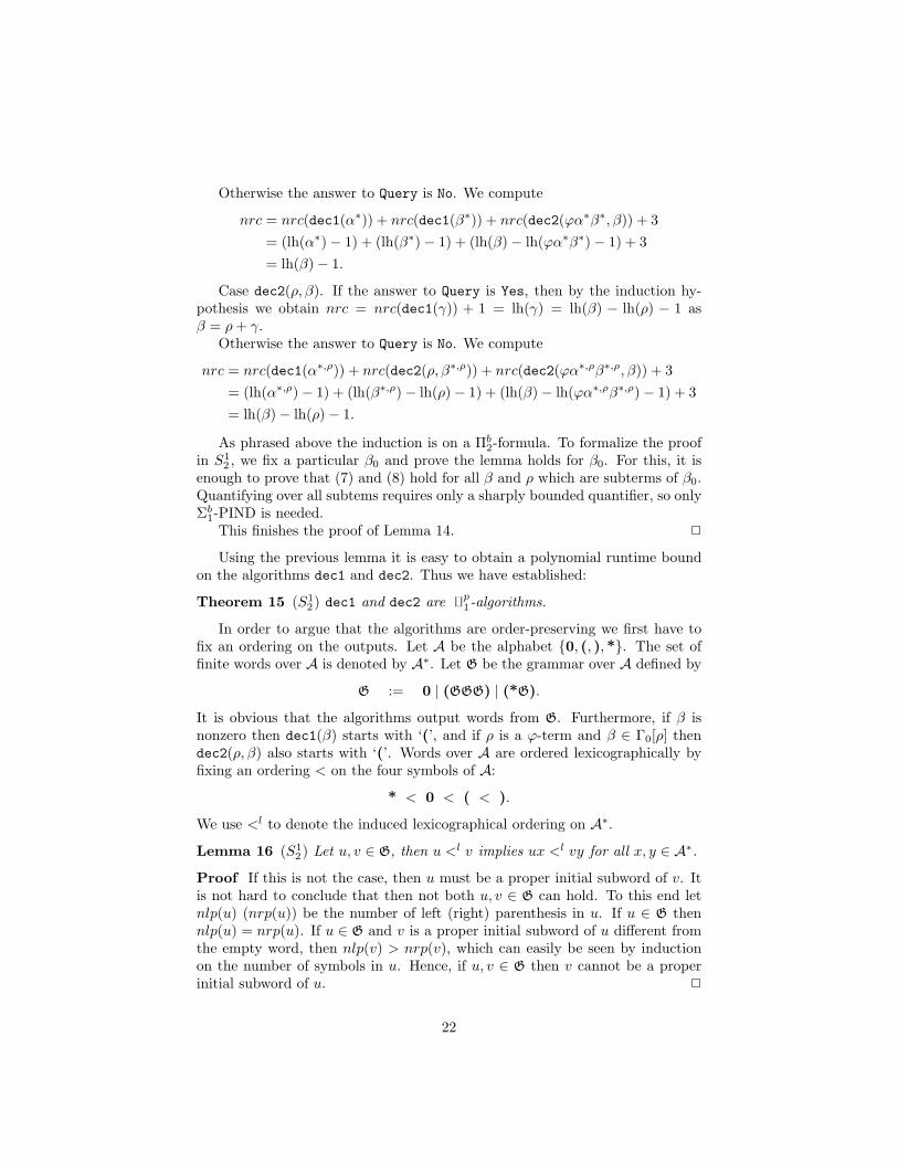
In order to argue that the algorithms are order-preserving we first have tofix an ordering on the outputs. Let A be the alphabet {0, (, ),*}. The set offinite words over A is denoted by A∗. Let G be the grammar over A defined by

G := 0 | (GGG) | (*G).

It is obvious that the algorithms output words from G. Furthermore, if β isnonzero then dec1(β) starts with ‘(’, and if ρ is a ϕ-term and β ∈ Γ0[ρ] thendec2(ρ, β) also starts with ‘(’. Words over A are ordered lexicographically byfixing an ordering < on the four symbols of A:

* < 0 < ( < ).

We use <l to denote the induced lexicographical ordering on A∗.

Lemma 16 (S12) Let u, v ∈ G, then u <l v implies ux <l vy for all x, y ∈ A∗.

Proof If this is not the case, then u must be a proper initial subword of v. Itis not hard to conclude that then not both u, v ∈ G can hold. To this end letnlp(u) (nrp(u)) be the number of left (right) parenthesis in u. If u ∈ G thennlp(u) = nrp(u). If u ∈ G and v is a proper initial subword of u different fromthe empty word, then nlp(v) > nrp(v), which can easily be seen by inductionon the number of symbols in u. Hence, if u, v ∈ G then v cannot be a properinitial subword of u. 2

22

We now show that S12 can prove that the algorithms compute order-

preserving maps.

Theorem 17 (S12) dec1 and dec2 are order-preserving.

In order to show this we will prove

1. Let β, η ∈ NF, then

β ≺ η ⇔ dec1(β) <l dec1(η).

2. Let ρ be a ϕ-term and β, η ∈ Γ0[ρ], then

β ≺ η ⇔ dec2(ρ, β) <l dec2(ρ, η).

In both cases it is enough to show “⇒”, e.g. because then

β 6≺ η ⇒ η 4 β ⇒ dec1(η) ≤l dec1(β) ⇒ dec1(β) 6<l dec1(η)

We show 1. and 2. simultaneously by induction on lh(β), respectively, lh(β)−lh(ρ). More exactly, as in the proof of Lemma 14, we show for all β, η, ρ occuringas subterms of some fixed β0, that if β ∈ NF then

lh(β) ≤ k ∧ β ≺ η ⇒ dec1(β) <l dec1(η),

and if ρ is a ϕ-term and β, η ∈ Γ0[ρ] then

lh(β) − lh(ρ) ≤ k ∧ β ≺ η ⇒ dec2(ρ, β) <l dec2(ρ, η)

by length-induction on k.For 1., assume β ≺ η. If β = 0 then

dec1(β) = 0 <l ( <l dec1(η).

Otherwise β 6= 0, and by Lemma 12, α∗ := m1(β) 4 m1(η) =: ξ∗.

A. If α∗ ≺ ξ∗ then the induction hypothesis shows dec1(α∗) <l dec1(ξ∗),hence the assertion follows using the previous lemma.

B. Otherwise α∗ = ξ∗, hence β∗ := m2(β) 4 m2(η) =: η∗ by Lemma 12.

(a) If β∗ ≺ η∗ then the induction hypothesis shows dec1(β∗) <l

dec1(η∗), hence the assertion follows again using the previousLemma.

(b) Otherwise β∗ = η∗. Let ρ := ϕα∗β∗ = ϕξ∗η∗. Hence β, η ∈ Γ0[ρ]by Lemma 9. The induction hypothesis now yields dec2(ρ, β) <l

dec2(ρ, η), hence the assertion follows.

For 2., let β, η ∈ Γ0[ρ], ρ some ϕ-term, and assume β ≺ η.

23

A. Assume β has the form ρ + γ.

(a) Assume η has the form ρ+δ. Then γ ≺ δ and by induction hypothesisdec1(γ) <l dec1(δ), hence the assertion follows.

(b) Otherwise η does not have the form ρ + δ. But then

dec2(ρ, β) = (* . . . <l (0 <l dec2(ρ, η).

B. Otherwise β is not of the form ρ + γ. By Lemma 11.2. it follows thatalso η is not of this form. Hence the answers to both Query’s are No.Furthermore, β, η ∈ Γ0[ρ], thus we can apply Lemma 13 to obtain α∗,ρ :=mρ

1(β) 4 mρ1(η) =: ξ∗,ρ.

(a) If α∗,ρ ≺ ξ∗,ρ then the induction hypothesis shows dec1(α∗,ρ) <l

dec1(ξ∗,ρ), hence the assertion follows.

(b) Otherwise α∗,ρ = ξ∗,ρ. Then β∗,ρ := mρ2(β) 4 mρ

2(η) =: η∗,ρ byLemma 13.

i. If β∗,ρ ≺ η∗,ρ then the induction hypothesis showsdec2(ρ, β∗,ρ) <l dec2(ρ, η∗,ρ), hence the assertion follows.

ii. Otherwise β∗,ρ = η∗,ρ. Let ρ := ϕα∗,ρβ∗,ρ = ϕξ∗,ρη∗,ρ. Henceβ, η ∈ Γ0[ρ] by Lemma 10. The induction hypothesis now yieldsdec2(ρ, β) <l dec2(ρ, η), hence the assertion follows.

That finishes the proof of Theorem 17.

Theorem 18 Let ≺ be the ordering on normal forms. Then T 12 ` WF≺.

Proof The task of finding a ≺-minimal β ≤ t with A(β), A ∈ Σb1, can now be

reduced to finding a <l-minimal n ≤ t′ such that

A∗(n) ≡ (∃β ≤ t)(dec1(β) = n ∧ A(β)) ∈ Σb1

holds. The bound t′ must be large enough so that dec1(β) ≤ t′ whenever β ≤ t;examination of the algorithms and Lemma 14 shows immediately that dec1(β)has length linearly bounded by lh(β), so t′ = tO(1) suffices. Using the sametechnique as in section 3 for coding fixed length words order-preserving intonatural numbers this task can be solved by Σb

1 − Min, which is at hand in T 12 .

2

5 Embedding into lexicographic orderings

Let A be a finite, ordered set of cardinality at least 2, and A∗ be the set of words(finite sequences) over A with the lexicographic ordering. Similarly, N∗ denotesthe set of finite sequences of non-negative integers ordered lexicographically. Theproofs of the Theorems 4 and 18 involved giving order-preserving embeddingsof notations for ordinals less than ε0 and Γ0 into N∗ or a set A∗. In this section,

24

we consider the question of how general these order preserving embeddings are,and whether they always must exist.

First, we prove a simple fact showing that N∗ can always be replaced by A∗.

Proposition 19 There is an order-preserving embedding of N∗ into A∗. Fur-thermore, this embedding is polynomial time computable.

Proof Without loss of generality, A has the symbols 0 < 1 as members. Ifn ≥ 0, let bn ∈ {0, 1}∗ be the binary representation of n. Let 1k be theword which consists of k 1’s. The desired embedding σ is defined by lettingσ(〈n1, n2, . . . , nk〉) equal 1|n1|0bn11

|n2|0bn2 · · · 1|nk|0bnk. It is easy to verify that

σ has the necessary properties. 2

Next we characterize which orderings can be embedded into A∗ in an order-preserving fashion. Note that A∗ is countable, so only countable orderings canbe embedded into A∗.

Theorem 20 Any countable ordering can be embedded into A∗.

Proof Obviously any finite ordering can be embedded into A∗. So it sufficesto assume that the ordering, denoted ≺, has domain the set N. Let A = {0, 1}.We shall define an ordering preserving embedding σ : N 7→ A∗. The values σ(n)will be defined so that they always end with the symbol 1, i.e., σ(n) is in theregular set (0 ∪ 1)∗1. Define pred(α1) = α01 and succ(α1) = α11. We let |α|denote the number of symbols in the word α.

Inductively define σ(n) as follows. First, σ(0) = 1. To define σ(n + 1),let i be the ≺-greatest element from {0, . . . , n} such that i ≺ (n + 1), if anysuch i exists, and dually let j be the ≺-least element from {0, . . . n} such thatj  (n + 1). In case i does not exist or σ(i) is a proper subsequence of σ(j),let σ(n + 1) = pred(σ(j)). Otherwise, j does not exist or σ(i) is not a propersubsequence of σ(j), and in this case σ(n + 1) = succ(σ(i)).

We leave to the reader the straightforward proofs that σ is one-to-one andorder-preserving. 2

The above proof immediately implies that if ≺ is recursive (respectively,polynomial time), then σ is recursive (respectively, exponential time). Becauseof the exponential time complexity, this general result is not good enough toimply anything about provability of well-orderings over bounded domains inbounded arithmetic.

6 Ordinal cost functions for PLS

The class PLS of polynomial local search functions was originally defined byJohnson, Papadimitriou and Yannakakis [9] and contains functions which searchfor a minimal cost (equivalently, maximal cost) feasible solution. Buss andKrajıcek [5] used this class to characterize the provably total functions of T 1

2 as

25

being the set of functions which can be defined as the composition of a projectionfunction and a PLS function.

We give a quick sketch of the definition of the class PLS and the reader canrefer to above references for more detailed definitions.

Definition A PLS problem consists of a cost function c, a neighborhood func-tion N , and a polynomially bounded set of feasible solutions, defined by apredicate F . For an input x, the set {s : F (x, s)} is the set of feasible solutions,the mapping s 7→ c(x, s) assigns a cost to each feasible solution, and the map-ping s 7→ N(x, s) maps feasible solutions to feasible solutions. The functions cand N and the predicate F must be polynomial time computable. The functiondefined by the PLS problem is the (multivalued) function f defined by f(x) = yiff F (x, y) and c(x,N(x, y)) 6< c(x, y).

We can generalize PLS to allow the cost function to take on ordinal valuesinstead of integer values. (It is for this reason that we defined PLS problemsas a minimization problems rather than maximization problems.) Let α denotean ordinal, such as ε0 or Γ0, with a system of ordinal notations so that theset of valid ordinal notations is polynomial time recognizable and so that theinduced ordering, 4, on ordinal notations is polynomial time. The class of(α,4)-PLS problems is defined identically to the class PLS except that thecondition c(x,N(x, y)) 6< c(x, y) is replaced by c(x,N(x, y)) 6≺ c(x, y).

We shall see below that PLS and (ε0,4)-PLS and (Γ0,4)-PLS are identicalin that they contain exactly the same functions. To establish this result in itsstrongest form we need the following proposition.

Proposition 21 Let h(x) be a (multivalued) function such that h = g ◦f whereg is a polynomial time function and f is a PLS function. Further suppose thatthe graph of h, {(x, y) : h(x) = y} is polynomial time. Then h is a PLS function.

Proof Let f be the PLS function defined by c, N and F . We must define c′,N ′ and F ′ that define the function h. These are defined as follows:

c′(x, s) ={

0 if h(x) = sc(x, s) + 1 otherwise

N ′(x, s) =

s if h(x) = sg(s) if h(x) = g(s) and h(x) 6= sN(x, s) otherwise

F ′(x, s) ⇔ F (x, s) ∨ h(x) = s

It is clear by inspection that c′, N ′ and F ′ define h as a PLS problem. 2

Theorem 22 The classes (ε0,4)-PLS and (Γ0,4)-PLS are both equal to PLS.

To prove this theorem, first note that any PLS function is clearly in (ε0,4)-PLS and in (Γ0,4)-PLS by using the construction from the proof of Theorem 3to transform integer values of a cost function into ordinal notations. For the

26

other direction, suppose that f is a function in (ε0,4)-PLS or (Γ0,4)-PLS. ByTheorem 4 or 18, T 1

2 can prove that for all inputs x, there is a feasible solution sof minimum cost, and hence of minimal cost. Therefore, by Buss-Krajıcek [5],f can be expressed as the composition of a projection function and a PLSfunction. Since the graph of f is polynomial time, Proposition 21 implies thatf is also a PLS function.

References

[1] A. Beckmann, Separating Fragments of Bounded Arithmetic, PhD thesis,Univ. of Munster, 1996.

[2] , Notations for exponentiation. Submitted for publication, 1999.

[3] S. R. Buss, Bounded Arithmetic, Bibliopolis, 1986. Revision of 1985Princeton University Ph.D. thesis.

[4] , Axiomatizations and conservation results for fragments of boundedarithmetic, in Logic and Computation, proceedings of a Workshop heldCarnegie-Mellon University, 1987, vol. 106 of Contemporary Mathematics,American Mathematical Society, 1990, pp. 57–84.

[5] S. R. Buss and J. Krajıcek, An application of Boolean complexity toseparation problems in bounded arithmetic, Proc. London Math. Society, 69(1994), pp. 1–21.

[6] S. Feferman, Systems of predicative analysis I, Journal of Symbolic Logic,29 (1964), pp. 1–30.

[7] , Systems of predicative analysis II: Representations of ordinals, Jour-nal of Symbolic Logic, 30 (1968), pp. 193–220.

[8] P. Hajek and P. Pudlak, Metamathematics of First-order Arithmetic,Perspectives in Mathematical Logic, Springer-Verlag, Berlin, 1993.

[9] D. S. Johnson, C. H. Papadimitriou, and M. Yannakakis, How easyis local search?, J. Comput. System Sci., 37 (1988), pp. 79–100.

[10] J. Krajıcek, Bounded Arithmetic, Propositional Calculus and ComplexityTheory, Cambridge University Press, 1995.

[11] W. Pohlers, Proof Theory: An Introduction, Lecture Notes in Mathe-matics, #1409, Springer-Verlag, Berlin, 1989.

[12] K. Schutte, Proof Theory, Grundlehren der mathematischen Wis-senschaften #225, Springer-Verlag, Berlin, 1977.

[13] R. Sommer, Transfinite Induction and Hierarchies Generated by Transfi-nite Recursion within Peano Arithmetic, PhD thesis, U.C. Berkeley, 1990.

27

[14] , Ordinal arithmetic in I∆0, in Arithmetic, Proof Theory and Com-putational Complexity, P. Clote and J. Krajıcek, eds., Oxford University(Clarendon) Press, 1993, pp. 320–363.

28