arX

iv:m

ath/

0608

119v

1 [

mat

h.G

M]

4 A

ug 2

006

Order in DSmT; definition ofcontinuous DSm models

Frederic Dambreville

Delegation Generale pour l’Armement, DGA/CEP/GIP/SRO

16 Bis, Avenue Prieur de la Cote d’Or

Arcueil, F 94114, France

Web: http://www.FredericDambreville.com

Email: http://email.FredericDambreville.com

Abstract. When implementing the DSmT, a difficulty may arise from the

possible huge dimension of hyperpower sets, which are indeed free struc-

tures. However, it is possible to reduce the dimension of these structures by

involving logical constraints. In this paper, the logical constraints will be

related to a predefined order over the logical propositions. The use of such

orders and their resulting logical constraints will ensure a great reduction

of the model complexity. Such results will be applied to the definition of

continuous DSm models. In particular, a simplified description of the con-

tinuous impreciseness is considered, based on impreciseness intervals of the

sensors. From this viewpoint, it is possible to manage the contradictions

between continuous sensors in a DSmT manner, while the complexity of the

model stays handlable.

1 Introduction

Recent advances[2] in the Dezert Smarandache Theory have shown that this

theory was able to handle the contradiction between propositions in a quite

flexible way. This new theory has been already applied in different domains;

e.g.:

• Data asociation in target tracking [3] ,

• Environmental prediction [4] .

Although free DSm models are defined over hyperpower sets, which sizes

evolve exponentially with the number of atomic propositions, it appears

1

that the manipulation of the fusion rule is still manageable for practical

problems reasonnably well shaped. Moreover, the hybrid DSm models are

of lesser complexity.

If DSmT works well for discret spaces, the manipulation of continous DSm

models is still an unknown. Nevertheless, the management of continuous

data is an issue of main interest. It is necessary for implementing a true

fusion engine for localization informations; and associated with a principle

of conditionning, it will be a main ingredient for implementing filters for the

localization. But a question first arises: what could be an hyperpower set for

a continuous DSm model? Such first issue does not arises so dramatically

in Dempster Shafer Theory or for Transfer Belief Models[5]. In DST, a con-

tinuous proposition could just be a measurable subset. On the other hand,

a free DSm model, defined over an hyperpower set, will imply that any pair

of propositions will have a non empty intersection. This is desappointing,

since the notion of point (a minimal non empty proposition) does not exist

anymore in an hyperpower set.

But even if it is possible to define a continuous propositional model in

DST/TBM, the manipulation of continuous basic belief assignment is still

an issue[6][7]. In [6] , Ristic and Smets proposed a restriction of the bba

to intervals of IR . It was then possible to derive a mathematical relation

between a continuous bba density and its Bel function.

In this paper, the construction of continuous DSm models is proposed. This

construction is based on a constrained model, where the logical contraints

are implied by the definition of an order relation over the propositions.

A one-dimension DSm model will be implemented, where the definition of

the basic belief assignment relies on a generalized notion of intervals. Al-

though this construction has been fulfilled on a different ground, it shares

some surprizing similarities with Ristic and Smets viewpoint. As in [6], the

bba will be seen as density defined over a 2-dimension measurable space. We

will be able to derive the Belief function from the basic belief assignment, by

applying an integral computation. At last, the conjunctive fusion operator,

⊕, is derived by a rather simple integral computation.

Section 2 makes a quick introduction of the Dezert Smarandache Theory.

2

Section 3 is about ordered DSm models. In section 4, a continuous DSm

model is defined. This method is restricted to only one dimension. The

related computation methods are detailed. In section 5, our algorithmic

implementation is described and an example of computation is given. The

paper is then concluded.

2 A short introduction to the DSmT

The theory and its meaning are widely explained in [2]. However, we will

particularly focus on the notion of hyperpower sets, since this notion is fun-

damental subsequently.

The Dezert Smarandache Theory belongs to the family of Evidence Theories.

As the Dempster Shafer Theory [8][9] or the Transferable Belief Models[5],

the DSmT is a framework for fusing belief informations, originating from

independent sensors. However, free DSm models are defined over Hyper-

power sets, which are fully open-world extensions of sets. It is possible to

restrict this full open-world hypothesis by adding propositional constraints,

resulting in the definition of an hybrid Dezert Smarandache model.

The notion of hyperpower set is thus a fundamental ingredient of the DSmT.

Hyperpower sets could be considered as a free pre-Boolean algebra. As these

structures will be of main importance subsequently, the next sections are de-

voted to introduce them in details. As a prerequisite, the notion of Boolean

algebra is quickly introduced now.

2.1 Boolean algebra

Definition. A Boolean algebra is a sextuple (Φ,∧,∨,¬,⊥,⊤) such that:

• Φ is a set, called set of propositions,

• ⊥,⊤ are specific propositions of Φ, respectively called false and true,

• ¬ : Φ → Φ is a unary operator,

• ∧ : Φ × Φ → Φ and ∨ : Φ × Φ → Φ are binary operators,

and verifying the following properties:

3

A1. ∧ and ∨ are commutative:

∀φ,ψ ∈ Φ, φ ∧ ψ = ψ ∧ φ and φ ∨ ψ = ψ ∨ φ ,

A2. ∧ and ∨ are associative:

∀φ,ψ, η ∈ Φ, (φ ∧ ψ) ∧ η = φ ∧ (ψ ∧ η) and (φ ∨ ψ) ∨ η = φ ∨ (ψ ∨ η) ,

A3. ⊤ is neutral for ∧ and ⊥ is neutral for ∨:

∀φ ∈ Φ, φ ∧⊤ = φ and φ ∨ ⊥ = φ ,

A4. ∧ and ∨ are distributive for each other:

∀φ,ψ, η ∈ Φ, φ∧(ψ∨η) = (φ∧ψ)∨(φ∧η) and φ∨(ψ∧η) = (φ∨ψ)∧(φ∨η) ,

A5. ¬ defines the complement of any proposition:

∀φ ∈ Φ, φ ∧ ¬φ = ⊥ and φ ∨ ¬φ = ⊤ .

The Boolean algebra (Φ,∧,∨,¬,⊥,⊤) will be also refered to as the Boolean

algebra Φ, the strucure being thus implied. An order relation ⊂ is defined

over Φ by:

∀φ,ψ ∈ Φ , φ ⊂ ψ∆

⇐⇒ φ ∧ ψ = φ .

Fundamental examples. The following examples are two main concep-

tions of Boolean algebra.

Example 1 Let Ω be a set and P(Ω) be the set of its subsets. For any

A ⊂ Ω, denote ∼ A = Ω \A its complement. Then (P(Ω),∩,∪,∼, ∅,Ω) is a

Boolean algebra.

The proof is immediate by verifying the properties A1 to A5.

Example 2 For any i ∈ 1, . . . , n, let θi = 0, 1i−1×0×0, 1n−i . Let

Θ = θ1, . . . , θn and denote ⊥ = ∅, ⊤ = 0, 1n and B(Θ) = P(0, 1n) .

Define the operators ∧, ∨ and ¬ by φ ∧ ψ = φ ∩ ψ, φ ∨ ψ = φ ∪ ψ and

¬φ = ⊤ \ φ for any φ,ψ ∈ B(Θ) . Then (B(Θ),∧,∨,¬,⊥,⊤) is a Boolean

algebra.

4

a

¬a

b ¬b

a ∧ b a ∧ ¬b

¬a ∧ b ¬a ∧ ¬b

a ∨ ¬b

¬a ∧ b

⊤

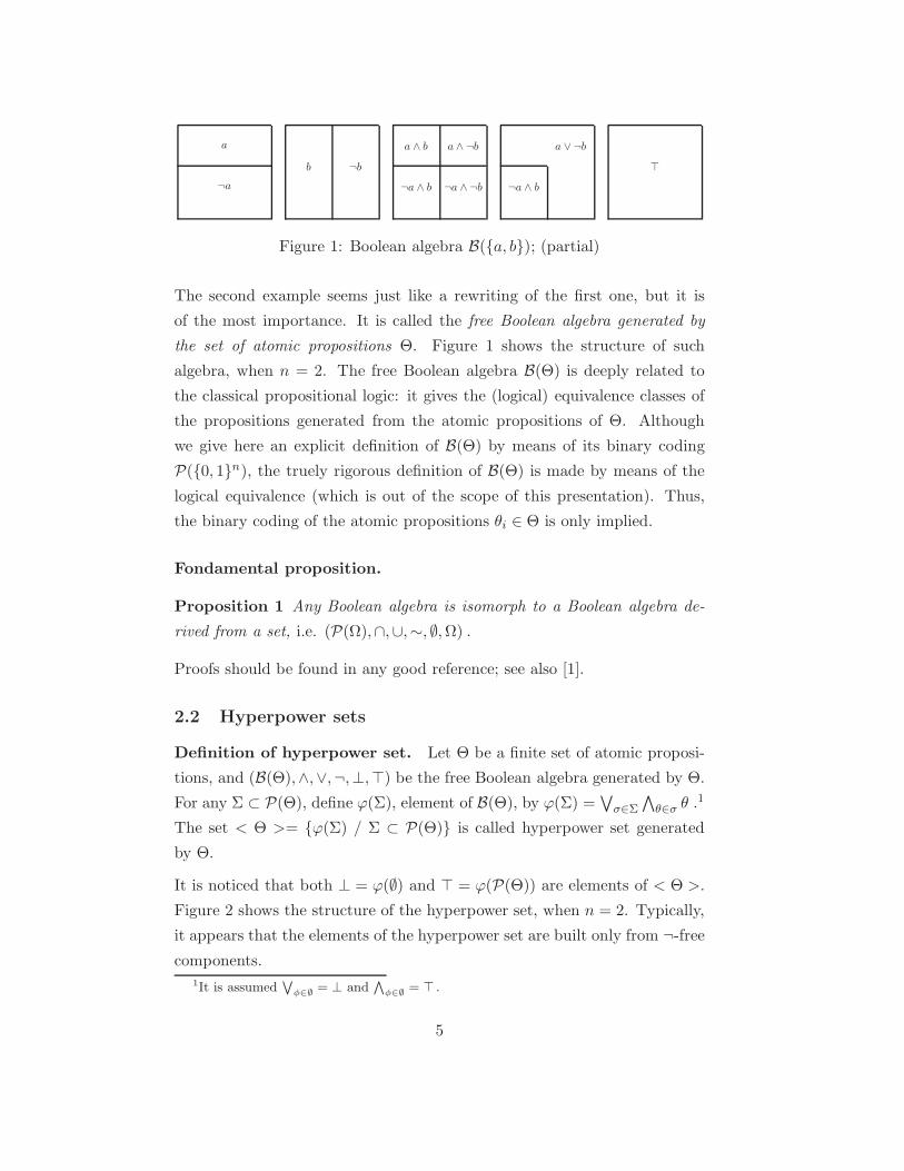
Figure 1: Boolean algebra B(a, b); (partial)

The second example seems just like a rewriting of the first one, but it is

of the most importance. It is called the free Boolean algebra generated by

the set of atomic propositions Θ. Figure 1 shows the structure of such

algebra, when n = 2. The free Boolean algebra B(Θ) is deeply related to

the classical propositional logic: it gives the (logical) equivalence classes of

the propositions generated from the atomic propositions of Θ. Although

we give here an explicit definition of B(Θ) by means of its binary coding

P(0, 1n), the truely rigorous definition of B(Θ) is made by means of the

logical equivalence (which is out of the scope of this presentation). Thus,

the binary coding of the atomic propositions θi ∈ Θ is only implied.

Fondamental proposition.

Proposition 1 Any Boolean algebra is isomorph to a Boolean algebra de-

rived from a set, i.e. (P(Ω),∩,∪,∼, ∅,Ω) .

Proofs should be found in any good reference; see also [1].

2.2 Hyperpower sets

Definition of hyperpower set. Let Θ be a finite set of atomic proposi-

tions, and (B(Θ),∧,∨,¬,⊥,⊤) be the free Boolean algebra generated by Θ.

For any Σ ⊂ P(Θ), define ϕ(Σ), element of B(Θ), by ϕ(Σ) =∨

σ∈Σ

∧

θ∈σ θ .1

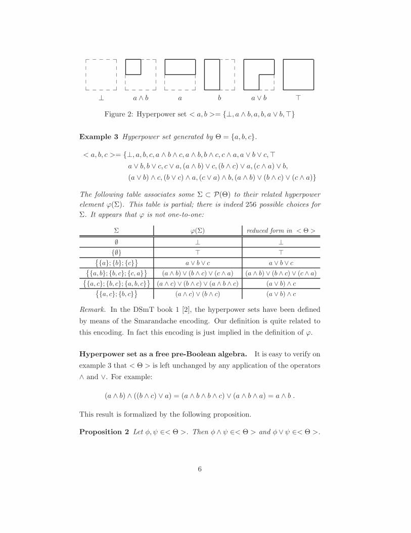
The set < Θ >= ϕ(Σ) / Σ ⊂ P(Θ) is called hyperpower set generated

by Θ.

It is noticed that both ⊥ = ϕ(∅) and ⊤ = ϕ(P(Θ)) are elements of < Θ >.

Figure 2 shows the structure of the hyperpower set, when n = 2. Typically,

it appears that the elements of the hyperpower set are built only from ¬-free

components.1It is assumed

∨

φ∈∅= ⊥ and

∧

φ∈∅= ⊤ .

5

_____

_____

___

_____

_____

___

___

___

⊥ a ∧ b a b a ∨ b ⊤

Figure 2: Hyperpower set < a, b >= ⊥, a ∧ b, a, b, a ∨ b,⊤

Example 3 Hyperpower set generated by Θ = a, b, c.

< a, b, c >= ⊥, a, b, c, a ∧ b ∧ c, a ∧ b, b ∧ c, c ∧ a, a ∨ b ∨ c,⊤

a ∨ b, b ∨ c, c ∨ a, (a ∧ b) ∨ c, (b ∧ c) ∨ a, (c ∧ a) ∨ b,

(a ∨ b) ∧ c, (b ∨ c) ∧ a, (c ∨ a) ∧ b, (a ∧ b) ∨ (b ∧ c) ∨ (c ∧ a)

The following table associates some Σ ⊂ P(Θ) to their related hyperpower

element ϕ(Σ). This table is partial; there is indeed 256 possible choices for

Σ. It appears that ϕ is not one-to-one:

Σ ϕ(Σ) reduced form in < Θ >

∅ ⊥ ⊥

∅ ⊤ ⊤

a; b; c

a ∨ b ∨ c a ∨ b ∨ c

a, b; b, c; c, a

(a ∧ b) ∨ (b ∧ c) ∨ (c ∧ a) (a ∧ b) ∨ (b ∧ c) ∨ (c ∧ a)

a, c; b, c; a, b, c

(a ∧ c) ∨ (b ∧ c) ∨ (a ∧ b ∧ c) (a ∨ b) ∧ c

a, c; b, c

(a ∧ c) ∨ (b ∧ c) (a ∨ b) ∧ c

Remark. In the DSmT book 1 [2], the hyperpower sets have been defined

by means of the Smarandache encoding. Our definition is quite related to

this encoding. In fact this encoding is just implied in the definition of ϕ.

Hyperpower set as a free pre-Boolean algebra. It is easy to verify on

example 3 that < Θ > is left unchanged by any application of the operators

∧ and ∨. For example:

(a ∧ b) ∧ ((b ∧ c) ∨ a) = (a ∧ b ∧ b ∧ c) ∨ (a ∧ b ∧ a) = a ∧ b .

This result is formalized by the following proposition.

Proposition 2 Let φ,ψ ∈< Θ >. Then φ∧ ψ ∈< Θ > and φ∨ ψ ∈< Θ >.

6

Proof. Let φ,ψ ∈< Θ >.

There are Σ ⊂ P(Θ) and Γ ⊂ P(Θ) such that φ = ϕ(Σ) and ψ = ϕ(Γ) .

By applying the definition of ϕ, it comes immediately:

ϕ(Σ) ∨ ϕ(Γ) =∨

σ∈Σ∪Γ

∧

θ∈σ

θ .

It is also deduced:

ϕ(Σ) ∧ ϕ(Γ) =

(

∨

σ∈Σ

∧

θ∈σ

θ

)

∧

(

∨

γ∈Γ

∧

θ∈γ

θ

)

.

By applying the distributivity, it comes:

ϕ(Σ) ∧ ϕ(Γ) =∨

σ∈Σ

∨

γ∈Γ

(

(

∧

θ∈σ

θ

)

∧

(

∧

θ∈γ

θ

)

)

=∨

(σ,γ)∈Σ×Γ

∧

θ∈σ∪γ

θ .

Then ϕ(Σ) ∧ ϕ(Γ) = ϕ(Λ) , with Λ = σ ∪ γ / (σ, γ) ∈ Σ × Γ .

Corollary and definition. Proposition 2 implies that ∧ and ∨ infer inner

operations within < Θ > . As a consequence, (< Θ >,∧,∨,⊥,⊤) is an

algebraic structure by itself. Since it does not contains the negation ¬, this

structure is called the free pre-Boolean algebra generated by Θ.

2.3 Pre-Boolean algebra

Generality. Typically, a free algebra is an algebra where the only con-

straints are the intrinsic contraints which characterize its fundamental struc-

tures. For example in a free Boolean algebra, the only constraints are A1

to A5, and there are no other constraints put on the propositions. But con-

versely, it is indeed possible to derive any algebra by constraining its free

counterpart. This will be our approach for defining pre-Boolean algebra in

general: a pre-Boolean algebra will be a constrained free pre-Boolean alge-

bra. Constraining a structure is a quite intuitive notion. However, a precise

mathematical definition needs the abstract notion of equivalence relations

and classes. Let us start with the intuition by introducing an example.

Example 4 Pre-Boolean algebra generated by Θ = a, b, c and constrained

by a ∧ b = a ∧ c and a ∧ c = b ∧ c.

7

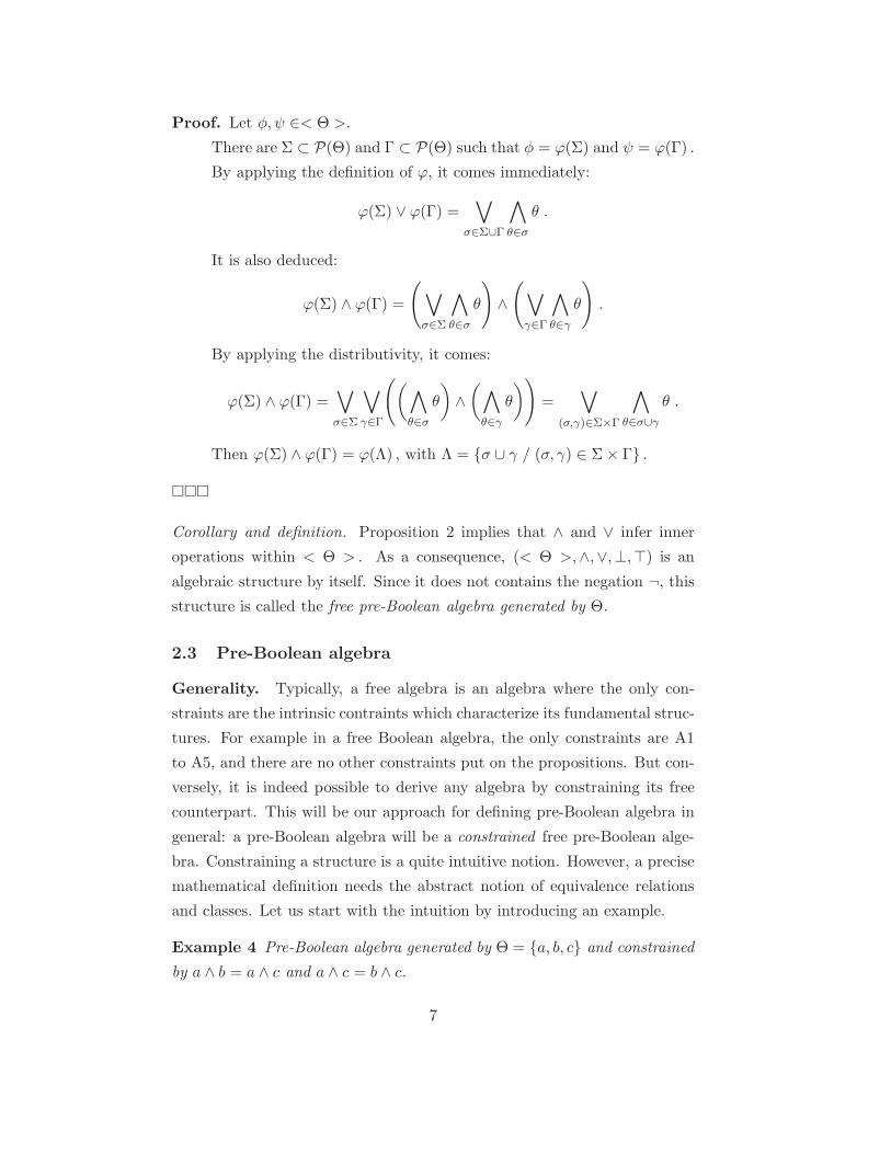
For coherence with forthcoming notations, these constraints will be desig-

nated by using the set of propositional pairs Γ = (a ∧ b, a ∧ c), (a ∧ c, b ∧ c) .

The idea is to start from the free pre-Boolean algebra < a, b, c >, propagate

the constraints, and then reduce the propositions identified by the constraints.

It is first deduced a ∧ b = a ∧ c = b ∧ c = a ∧ b ∧ c.

It follows (a ∧ b) ∨ c = c, (b ∧ c) ∨ a = a and (c ∧ a) ∨ b = b.

Also holds (a∨b)∧c = (b∨c)∧a = (c∨a)∧b = (a∧b)∨(b∧c)∨(c∧a) = a∧b∧c .

By discarding these cases from the free structure < a, b, c >, it comes the

following constrained pre-Boolean algebra:

< a, b, c >Γ= ⊥, a ∧ b ∧ c, a, b, c, a ∨ b, b ∨ c, c ∨ a, a ∨ b ∨ c,⊤

Of course, it is necessary to show that there is actually no further reduction

in < a, b, c >Γ. This is done by expliciting a model; for example the structure

of figure 3.

_____

2

22

222

___11

11

1

___

1111

1

22222

222

___11

11

1

___

1111

1

_____

2

22

22222

11

11

1

___

1111

1

_____

2

22

222

___1111111111

a ∧ b ∧ c a b c

22222

22222

11

11

1

___

1111

1

_____

2

22

22222

1111111111

22222

222

___1111111111

22222

22222

1111111111

a ∨ b b ∨ c c ∨ a a ∨ b ∨ c

Figure 3: Pre-Boolean algebra < a, b, c >Γ; (⊥ and ⊤ are omitted)

For the reader not familiar with the notion of equivalence classes, the fol-

lowing construction is just a mathematical formalization of the contraint

propagation which has been described in example 4. Now, it is first intro-

duced the notion of morphism between structures.

Magma. A (∧,∨,⊥,⊤)-magma, also called magma for short, is a quin-

tuple (Φ,∧,∨,⊥,⊤) where Φ is a set of propositions, ∧ and ∨ are binary

8

operators on Φ, and ⊥ and ⊤ are two elements of Φ.

The magma (Φ,∧,∨,⊥,⊤) may also be refered to as the magma Φ, the

structure being thus implied. Notice that an hyperpower set is a magma.

Morphism. Let (Φ,∧,∨,⊥,⊤) and (Ψ,∧,∨,⊥,⊤) be two magma. A mor-

phism µ from the magma Φ to the magma Ψ is a mapping from Φ to Ψ such

that:

• µ(φ ∧ ψ) = µ(φ) ∧ µ(ψ) and µ(φ ∨ ψ) = µ(φ) ∨ µ(ψ) ,

• µ(⊥) = ⊥ and µ(⊤) = ⊤ .

A morphism is an isomorphism if it is a bijective mapping. In such case,

the magma Φ and the magma Ψ are said to be isomorph, which means that

they share the same structure.

The notions of (∧,∨)-magma and of (∧,∨)-morphism are defined similarly

by discarding ⊥ and ⊤.

Propagation relation. Let < Θ > be a free pre-Boolean algebra. Let

Γ ⊂< Θ > × < Θ > be a set of propositional pairs; for any pair (φ,ψ) ∈ Γ

is defined the constraint φ = ψ . The propagation relation associated to the

constraints, and also denoted Γ, is defined recursively by:

• φΓφ, for any φ ∈< Θ >,

• If (φ,ψ) ∈ Γ, then φΓψ and ψΓφ,

• If φΓψ and ψΓη, then φΓη,

• If φΓη and ψΓζ, then (φ ∧ ψ)Γ(η ∧ ζ) and (φ ∨ ψ)Γ(η ∨ ζ)

The relation Γ is thus obtained by propagating the constraint over < Θ >.

It is obviously reflexive, symmetric and transitive; it is an equivalence rela-

tion. An equivalence class for Γ contains propositions which are identical in

regards to the constraints.

It is now time to define the pre-Boolean algebra.

9

Pre-Boolean algebra.

Proposition 3 Let be given a free pre-Boolean algebra < Θ > and a set of

propositional pairs Γ ⊂< Θ > × < Θ > . Then, there is a magma denoted

< Θ >Γ and a morphism µ :< Θ >→< Θ >Γ such that:

µ(< Θ >) =< Θ >Γ ,

∀φ,ψ ∈< Θ >, µ(φ) = µ(ψ) ⇐⇒ φΓψ .

The magma < Θ >Γ is called the pre-Boolean algebra generated by Θ and

constrained by the constraints φ = ψ where (φ,ψ) ∈ Γ .

Proof. For any φ ∈< Θ >, define φΓ = ψ ∈< Θ > / ψΓφ; this set is

called the class of φ for Γ .

It is a well known fact, and the proof is immediate, that φΓ = ψΓ or

φΓ ∩ ψΓ = ∅ for any φ,ψ ∈< Θ > ; in particular, φΓ = ψΓ ⇐⇒ φΓψ .

Now, assume ηΓ = φΓ and ζΓ = ψΓ, that is ηΓφ and ζΓψ.

It comes (η ∧ ζ)Γ(φ ∧ ψ) and (η ∨ ζ)Γ(φ ∨ ψ).

As a consequence, (η ∧ ζ)Γ = (φ ∧ ψ)Γ and (η ∨ ζ)Γ = (φ ∨ ψ)Γ.

At last:

(

ηΓ = φΓ and ζΓ = ψΓ

)

⇒(

(η∧ζ)Γ = (φ∧ψ)Γ and (η∨ζ)Γ = (φ∨ψ)Γ

)

The proof is then concluded easily, by setting:

< Θ >Γ= φΓ / φ ∈< Θ > ,

∀φ,ψ ∈< Θ >, φΓ ∧ ψΓ = (φ ∧ ψ)Γ and φΓ ∨ ψΓ = (φ ∨ ψ)Γ ,

∀φ ∈< Θ >, µ(φ) = φΓ .

From now on, the element µ(φ), where φ ∈< Θ >, will be denoted φ as if φ

were an element of < Θ >Γ . In particular, µ(φ) = µ(ψ) will imply φ = ψ

in < Θ >Γ (but not in < Θ >).

Proposition 4 Let be given a free pre-Boolean algebra < Θ > and a set of

propositional pairs Γ ⊂< Θ > × < Θ > . Let < Θ >Γ and < Θ >′Γ be pre-

Boolean algebras generated by Θ and constrained by the familly Γ . Then

< Θ >Γ and < Θ >′Γ are isomorph.

10

Proof. Let µ :< Θ >→< Θ >Γ and µ′ :< Θ >→< Θ >′Γ be as defined in

proposition 3.

For any φ ∈< Θ >, define ν(µ(φ)) = µ′(φ) .

Then, ν(µ(φ)) = ν(µ(ψ)) implies µ′(φ) = µ′(ψ) .

By definition of µ′, it is derived φΓψ and then µ(φ) = µ(ψ) .

Thus, ν is one-to-one.

By definition, it is also implied that ν is onto.

This property thus says that there is a structural unicity of < Θ >Γ .

Example 5 Let us consider again the pre-Boolean algebra generated by

Θ = a, b, c and constrained by a ∧ b = a ∧ c and a ∧ c = b ∧ c. In this case,

the mapping µ :< Θ >→< Θ >Γ is defined by:

• µ(⊥) = ⊥, µ(

a, (b ∧ c) ∨ a)

= a, µ(

b, (c ∧ a) ∨ b)

= b,

µ(

c, (a∧ b)∨ c)

= c, µ(a∨ b∨ c) = a∨ b∨ c, µ(⊤) = ⊤ ,

• µ(a ∨ b) = a ∨ b, µ(b ∨ c) = b ∨ c, µ(c ∨ a) = c ∨ a ,

• µ(

a ∧ b ∧ c, a ∧ b, b ∧ c, c ∧ a, (a ∨ b) ∧ c, (b ∨ c) ∧ a, (c ∨ a) ∧ b,

(a ∧ b) ∨ (b ∧ c) ∨ (c ∧ a))

= a ∧ b ∧ c .

Between sets and hyperpower sets.

Proposition 5 The Boolean algebra (P(Θ),∩,∪,∼, ∅,Θ), considered as a

(∧,∨,⊥,⊤)-magma, is isomorph to the pre-Boolean algebra < Θ >Γ, where

Γ is defined by:

Γ = (θ ∧ ϑ,⊥) / θ, ϑ ∈ Θ and θ 6= ϑ ∪

(

∨

θ∈Θ

θ,⊤

)

.

Proof. Recall the notation ϕ(Σ) =∨

σ∈Σ

∧

θ∈σ θ for any Σ ⊂ P(Θ) .

Define µ :< Θ >→ P(Θ) by setting2 µ(ϕ(Σ)) =⋃

σ∈Σ

⋂

θ∈σθ for

any Σ ⊂ P(Θ) .

It is immediate that µ is a morphism.

Now, by definition of Γ, µ(ϕ(Σ)) = µ(ϕ(Λ)) is equivalent to ϕ(Σ)Γϕ(Λ) .

The proof is then concluded by proposition 4.2It is defined

⋂

θ∈∅θ = Θ .

11

Thus, sets, considered as Boolean algebra, and hyperpower sets are both

extremal cases of the notion of pre-Boolean algebra. But while hyperpower

sets extend the structure of sets, hyperpower sets are more complexe in

structure and size than sets. A practical use of hyperpower sets becomes

quickly impossible. Pre-Boolean algebra however allows intermediate struc-

tures between sets and hyperpower sets.

A specific kind of pre-Boolean algebra will be particularly interesting when

defining the DSmT. Such pre-Boolean algebra will forbid any interaction

between the trivial propositions ⊥,⊤ and the other propositions. These

algebra, called insulated pre-Boolean algebra, are characterized now.

Insulated pre-Boolean algebra. A pre-Boolean algebra < Θ >Γ verifies

the insulation property if Γ ⊂ (< Θ > \⊥,⊤)) × (< Θ > \⊥,⊤)) .

Proposition 6 Let < Θ >Γ a pre-Boolean algebra verifying the insulation

property. Then holds for any φ,ψ ∈< Θ >Γ :

φ ∧ ψ = ⊥ ⇒ (φ = ⊥ or ψ = ⊥) ,

φ ∨ ψ = ⊤ ⇒ (φ = ⊤ or ψ = ⊤) .

In other words, all propositions are independent with each other in a pre-

Boolean algebra with insulation property.

The proof is immediate, since it is impossible to obtain φ∧ψΓ⊥ or φ∨ψΓ⊤

without involving ⊥ or ⊤ in the constraints of Γ. Examples 3 and example 4

verify the insulation property. On the contrary, a non empty set does not.

Corollary and definition. Let < Θ >Γ be a pre-Boolean algebra, verifying

the insulation property. Define ≪ Θ ≫Γ=< Θ >Γ \⊥,⊤ . The operators

∧ and ∨ restrict to ≪ Θ ≫Γ , and (≪ Θ ≫Γ,∧,∨) is an algebraic structure

by itself, called insulated pre-Boolean algebra. This structure is also refered

to as the insulated pre-Boolean algebra ≪ Θ ≫Γ.

Proposition 7 Let < Θ >Γ and < Θ >′Γ be pre-Boolean algebras with in-

sulation properties. Assume that the insulated pre-Boolean algebra ≪ Θ ≫Γ

and ≪ Θ ≫′Γ are (∧,∨)-isomorph. Then < Θ >Γ and < Θ >′

Γ are isomorph.

12

Deduced from the insulation property.

All ingredients are now gathered for the definition of Dezert Smarandache

models.

2.4 The free Dezert Smarandache Theory

Dezert Smarandache Model. Assume that Θ is a finite set. A Dezert

Smarandache model (DSmm) is a pair (Θ,m), where Θ is a set of proposi-

tions and the basic belief assignment m is a non negatively valued function

defined over < Θ > such that:

∑

φ∈<Θ>

m(φ) = 1 and m(⊥) = 0 .

Moreover, it is generally assumed that∑

φ∈≪Θ≫m(φ) = 1 , which means

that the propositions of Θ are exhaustive.

Belief Function. Assume that Θ is a finite set. The belief function Bel

related to a bba m is defined by:

∀φ ∈< Θ >, Bel(φ) =∑

ψ∈<Θ>:ψ⊂φ

m(ψ) . (1)

The equation (1) is invertible:

∀φ ∈< Θ >, m(φ) = Bel(φ) −∑

ψ∈<Θ>:ψ(φ

m(ψ) .

Fusion rule. Assume that Θ is a finite set. For a given universe Θ , and

two basic belief assignments m1 and m2, associated to independent sensors,

the fused basic belief assignment is m1 ⊕m2 , defined by:

m1 ⊕m2(φ) =∑

ψ1,ψ2∈<Θ>:ψ1∧ψ2=φ

m1(ψ1)m2(ψ2) . (2)

Remarks. It appears obviously that the previous definitions could be

equivalently restricted to ≪ Θ ≫, owing to the insulation properties.

Considering the definition of the fusion rule and the insulation property

(φ 6= ⊥ and ψ 6= ⊥) ⇒ (φ ∧ ψ) 6= ⊥, it appears also that these definitions

could be generalized to any algebra < Θ >Γ with the insulation property.

13

2.5 Extensions to any insulated pre-Boolean algebra

Let ≪ Θ ≫Γ be an insulated pre-Boolean algebra. The definition of bba

m, belief Bel and fusion ⊕ is thus kept unchanged (except the condition

m(⊥) = m(⊤) = 0 which become useless).

• A basic belief assignment m is a non negatively valued function defined

over ≪ Θ ≫Γ such that:

∑

φ∈≪Θ≫Γ

m(φ) = 1 .

• The belief function Bel related to a bba m is defined by:

∀φ ∈≪ Θ ≫Γ, Bel(φ) =∑

ψ∈≪Θ≫Γ:ψ⊂φ

m(ψ) .

• Being given two basic belief assignments m1 and m2, the fused basic

belief assignment m1 ⊕m2 is defined by:

m1 ⊕m2(φ) =∑

ψ1,ψ2∈≪Θ≫Γ:ψ1∧ψ2=φ

m1(ψ1)m2(ψ2) .

These extended definitions will be applied subsequently.

3 Ordered DSm model

From now on, we are working only with insulated pre-Boolean structures.

In order to reduce the complexity of the free DSm model, it is necessary

to introduce logical constraints which will lower the size of the pre-Boolean

algebra. Such constraints may appear clearly in the hypotheses of the prob-

lem. In this case, constraints come naturally and approximations may not

be required. However, when the model is too complex and there are no

explicit constraints for reducing this complexity, it is necessary to approxi-

mate the model by introducing some new constraints. Two rules should be

applied then:

• Only weaken informations3; do not produce information from nothing,

3Typically, a constraint like φ∧ ψ ∧ η = φ∧ ψ will weaken the information, by erasing

η from φ ∧ ψ ∧ η .

14

• minimize the information weakening.

First point garantees that the approximation does not introduce false infor-

mation. But some significant informations (eg. contradictions) are possibly

missed. This drawback should be avoided by second point.

In order to build a good approximation policy, some external knowledge,

like distance or order relation among the propositions could be used. Be-

hind these relations will be assumed some kind of distance between the

informations: more are the informations distant, more are their conjunctive

combination valuable.

3.1 Ordered atomic propositions

Let (Θ,≤) be an ordered set of atomic propositions. This order relation

is assumed to describe the relative distance between the information. For

example, the relation φ ≤ ψ ≤ η implies that φ and ψ are closer informations

than φ and η . Thus, the information contained in φ∧η is stronger than the

information contained in φ∧ψ . Of course, this comparison does not matter

when all the information is kept, but when approximations are necessary, it

will be useful to be able to choose the best information.

Sketchy example. Assume that 3 independent sensors are giving 3 mea-

sures about a continuous parameter, that is x, y and z. The parameters

x, y, z are assumed to be real values, not of the set IR but of its pre-Boolean

extension (theoretical issues will be clarified later4). The fused information

could be formalized by the proposition x∧y∧z (in a DSmT viewpoint). What

happen if we want to reduce the information by removing a proposition. Do

we keep x ∧ y , y ∧ z or x ∧ z ? This is of course an information weakening.

But it is possible that one information is better than an other. At this stage,

the order between the values x, y, z will be involved. Assume for example

that x ≤ y < z . It is clear that the proposition x ∧ z indicates a greater

contradiction than x∧y or y∧z . Thus, the proposition x∧z is the one which

should be kept! The discarding constraint x ≤ y ≤ z ⇒ x ∧ y ∧ z = x ∧ z is

implied then.

4In particular, as we are working in a pre-Boolean algebra, x ∧ y makes sense and it is

possible that x ∧ y 6= ⊥ even when x 6= y .

15

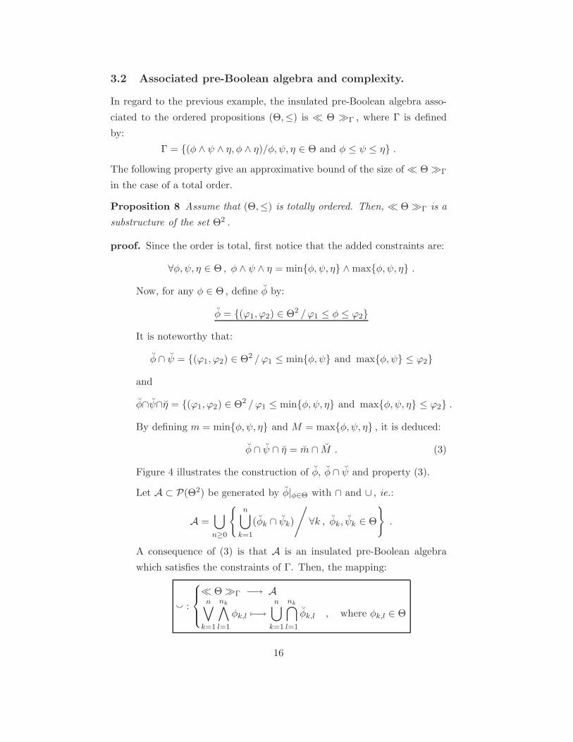
3.2 Associated pre-Boolean algebra and complexity.

In regard to the previous example, the insulated pre-Boolean algebra asso-

ciated to the ordered propositions (Θ,≤) is ≪ Θ ≫Γ , where Γ is defined

by:

Γ = (φ ∧ ψ ∧ η, φ ∧ η)/φ,ψ, η ∈ Θ and φ ≤ ψ ≤ η .

The following property give an approximative bound of the size of ≪ Θ ≫Γ

in the case of a total order.

Proposition 8 Assume that (Θ,≤) is totally ordered. Then, ≪ Θ ≫Γ is a

substructure of the set Θ2 .

proof. Since the order is total, first notice that the added constraints are:

∀φ,ψ, η ∈ Θ , φ ∧ ψ ∧ η = minφ,ψ, η ∧ maxφ,ψ, η .

Now, for any φ ∈ Θ, define φ by:

φ = (ϕ1, ϕ2) ∈ Θ2 /ϕ1 ≤ φ ≤ ϕ2

It is noteworthy that:

φ ∩ ψ = (ϕ1, ϕ2) ∈ Θ2 /ϕ1 ≤ minφ,ψ and maxφ,ψ ≤ ϕ2

and

φ∩ψ∩η = (ϕ1, ϕ2) ∈ Θ2 /ϕ1 ≤ minφ,ψ, η and maxφ,ψ, η ≤ ϕ2 .

By defining m = minφ,ψ, η and M = maxφ,ψ, η , it is deduced:

φ ∩ ψ ∩ η = m ∩ M . (3)

Figure 4 illustrates the construction of φ, φ ∩ ψ and property (3).

Let A ⊂ P(Θ2) be generated by φ|φ∈Θ with ∩ and ∪ , ie.:

A =⋃

n≥0

n⋃

k=1

(φk ∩ ψk)

/

∀k , φk, ψk ∈ Θ

.

A consequence of (3) is that A is an insulated pre-Boolean algebra

which satisfies the constraints of Γ. Then, the mapping:

` :

≪ Θ ≫Γ −→ An∨

k=1

nk∧

l=1

φk,l 7−→n⋃

k=1

nk⋂

l=1

φk,l , where φk,l ∈ Θ

16

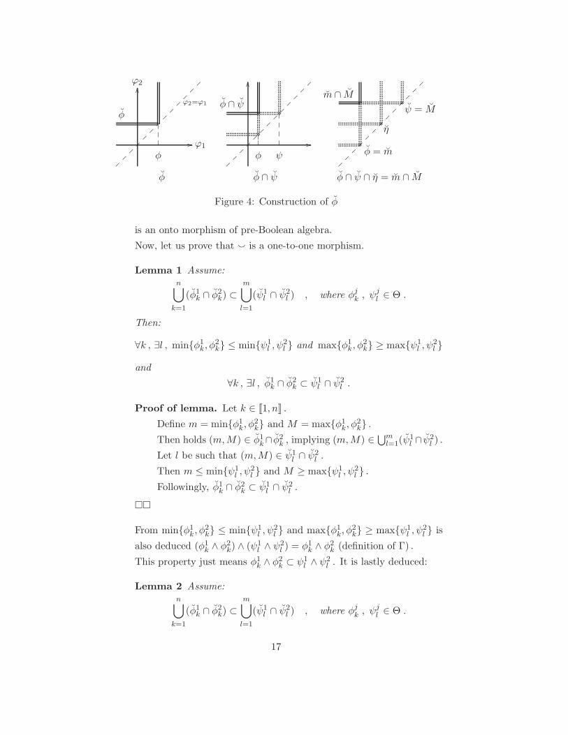
ϕ1

ϕ2

ϕ2=ϕ1

φ

φ

//

OO

φ ψ

φ ∩ ψ

//

OO

φ = m

η

ψ = M

m ∩ M

φ φ ∩ ψ φ ∩ ψ ∩ η = m ∩ M

Figure 4: Construction of φ

is an onto morphism of pre-Boolean algebra.

Now, let us prove that ` is a one-to-one morphism.

Lemma 1 Assume:

n⋃

k=1

(φ1k ∩ φ

2k) ⊂

m⋃

l=1

(ψ1l ∩ ψ

2l ) , where φjk , ψ

jl ∈ Θ .

Then:

∀k , ∃l , minφ1k, φ

2k ≤ minψ1

l , ψ2l and maxφ1

k, φ2k ≥ maxψ1

l , ψ2l

and

∀k , ∃l , φ1k ∩ φ

2k ⊂ ψ1

l ∩ ψ2l .

Proof of lemma. Let k ∈ [[1, n]] .

Define m = minφ1k, φ

2k and M = maxφ1

k, φ2k .

Then holds (m,M) ∈ φ1k∩ φ

2k , implying (m,M) ∈

⋃ml=1(ψ

1l ∩ ψ

2l ) .

Let l be such that (m,M) ∈ ψ1l ∩ ψ

2l .

Then m ≤ minψ1l , ψ

2l and M ≥ maxψ1

l , ψ2l .

Followingly, φ1k ∩ φ

2k ⊂ ψ1

l ∩ ψ2l .

From minφ1k, φ

2k ≤ minψ1

l , ψ2l and maxφ1

k, φ2k ≥ maxψ1

l , ψ2l is

also deduced (φ1k ∧ φ

2k) ∧ (ψ1

l ∧ ψ2l ) = φ1

k ∧ φ2k (definition of Γ) .

This property just means φ1k ∧ φ

2k ⊂ ψ1

l ∧ ψ2l . It is lastly deduced:

Lemma 2 Assume:

n⋃

k=1

(φ1k ∩ φ

2k) ⊂

m⋃

l=1

(ψ1l ∩ ψ

2l ) , where φjk , ψ

jl ∈ Θ .

17

Then:n∨

k=1

(φ1k ∧ φ

2k) ⊂

m∨

l=1

(ψ1l ∧ ψ

2l ) .

From this lemma, it is deduced that ` is one to one.

At last ` is an isomorphism of pre-Boolean algebra, and ≪ Θ ≫Γ is

a substructure of Θ2 .

3.3 General properties of the model

In the next section, the previous construction will be extended to the con-

tinuous case, ie. (IR,≤) . However, a strict logical manipulation of the

propositions is not sufficient and instead a measurable generalization of the

model will be used. It has been seen that a proposition of ≪ Θ ≫Γ could be

described as a subset of Θ2 . In this subsection, the proposition model will

be characterized precisely. This characterization will be used and extended

in the next section to the continuous case.

Proposition 9 Let φ ∈≪ Θ ≫Γ .

Then `(φ) ⊂ T , where T = (φ,ψ) ∈ Θ2/φ ≤ ψ .

Proof. Obvious, since ∀φ ∈ Θ , φ ⊂ T .

Definition 1 A subset θ ⊂ Θ2 is increasing if and only if:

∀ (φ,ψ) ∈ θ , ∀η ≤ φ , ∀ζ ≥ ψ , (η, ζ) ∈ θ .

Let U = θ ⊂ T /θ is increasing and θ 6= ∅ be the set of increasing non-

empty subsets of T . Notice that the intersection or the union of increasing

non-empty subsets are increasing non-empty subsets, so that (U ,∩,∪) is an

insulated pre-Boolean algebra.

Proposition 10 For any choice of Θ , `(φ)/φ ∈≪ Θ ≫Γ ⊂ U .

When Θ is finite, U = `(φ)/φ ∈≪ Θ ≫Γ .

Proof of ⊃ . Obvious, since φ is inceasing for any φ ∈ Θ .

18

Proof of ⊂ . Let θ ∈ U and let (a, b) ∈ θ .

Since a ∩ b = (α, β) ∈ Θ2/α ≤ a and β ≥ b and θ is increasing, it

follows a ∩ b ⊂ θ .

At last, θ =⋃

(a,b)∈θ a ∩ b =`

(

∨

(a,b)∈θ a ∧ b)

.

Notice that∨

(a,b)∈θ a ∧ b is actually defined, since θ is finite when Θ

is finite.

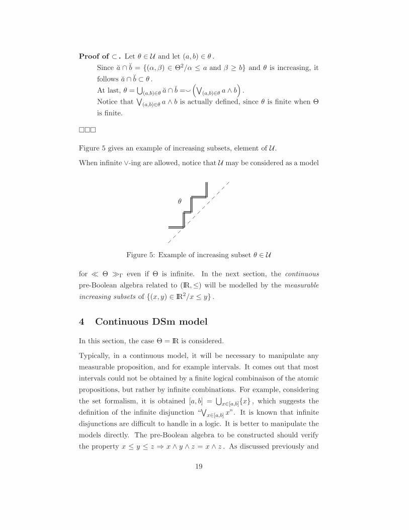
Figure 5 gives an example of increasing subsets, element of U .

When infinite ∨-ing are allowed, notice that U may be considered as a model

θ

Figure 5: Example of increasing subset θ ∈ U

for ≪ Θ ≫Γ even if Θ is infinite. In the next section, the continuous

pre-Boolean algebra related to (IR,≤) will be modelled by the measurable

increasing subsets of (x, y) ∈ IR2/x ≤ y .

4 Continuous DSm model

In this section, the case Θ = IR is considered.

Typically, in a continuous model, it will be necessary to manipulate any

measurable proposition, and for example intervals. It comes out that most

intervals could not be obtained by a finite logical combinaison of the atomic

propositions, but rather by infinite combinations. For example, considering

the set formalism, it is obtained [a, b] =⋃

x∈[a,b]x , which suggests the

definition of the infinite disjunction “∨

x∈[a,b] x”. It is known that infinite

disjunctions are difficult to handle in a logic. It is better to manipulate the

models directly. The pre-Boolean algebra to be constructed should verify

the property x ≤ y ≤ z ⇒ x ∧ y ∧ z = x ∧ z . As discussed previously and

19

since infinitary disjunctions are allowed, a model for such algebra are the

measurable increasing subsets.

4.1 Measurable increasing subsets

A measurable subset A ⊂ IR2 is a measurable increasing subset if:

∀ (x, y) ∈ A , x ≤ y ,

∀ (x, y) ∈ A , ∀a ≤ x , ∀b ≥ y , (a, b) ∈ A .

The set of measurable increasing subsets is denoted U .

Example. Let f : IR → IR be a non decreasing measurable mapping

such that f(x) ≥ x for any x ∈ IR. The set (x, y) ∈ IR2/f(x) ≤ y is a

measurable increasing subset.

“Points”. For any x ∈ IR, the measurable increasing subset x is defined

by:

x = (a, b) ∈ IR2 / a ≤ x ≤ b .

The set x is of course a model for the point x ∈ IR within the pre-Boolean

algebra (refer to section 3).

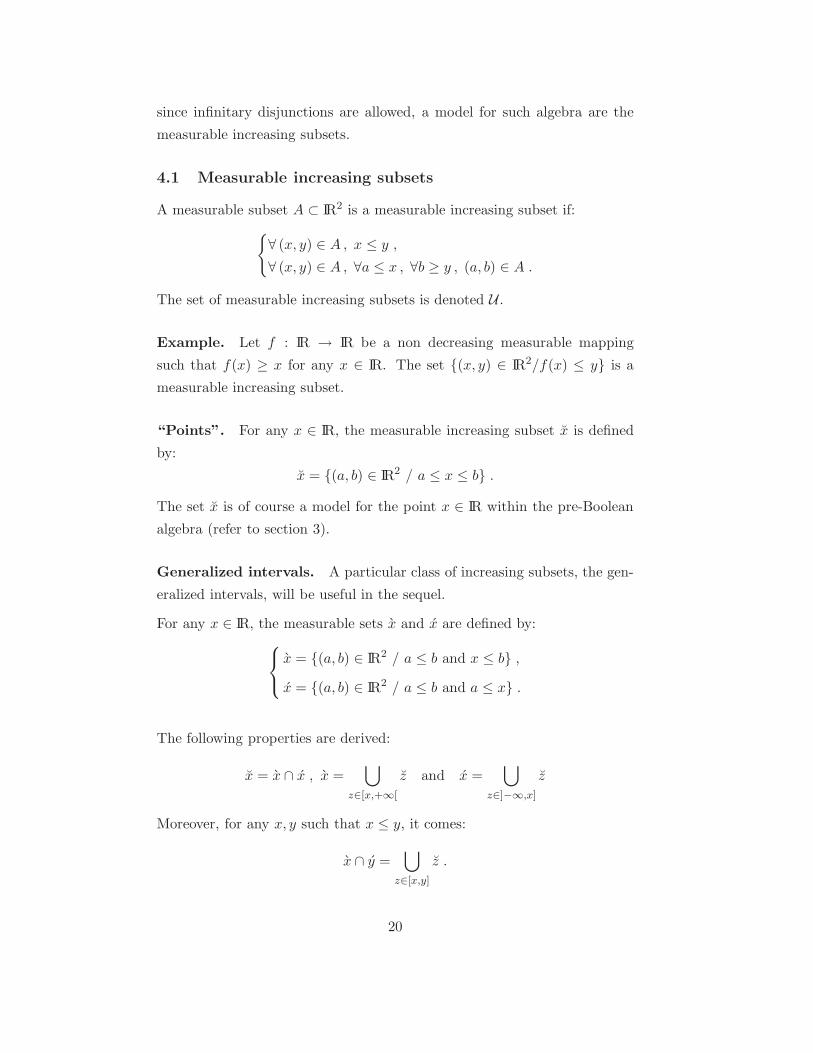
Generalized intervals. A particular class of increasing subsets, the gen-

eralized intervals, will be useful in the sequel.

For any x ∈ IR, the measurable sets x and x are defined by:

x = (a, b) ∈ IR2 / a ≤ b and x ≤ b ,

x = (a, b) ∈ IR2 / a ≤ b and a ≤ x .

The following properties are derived:

x = x ∩ x , x =⋃

z∈[x,+∞[

z and x =⋃

z∈]−∞,x]

z

Moreover, for any x, y such that x ≤ y, it comes:

x ∩ y =⋃

z∈[x,y]

z .

20

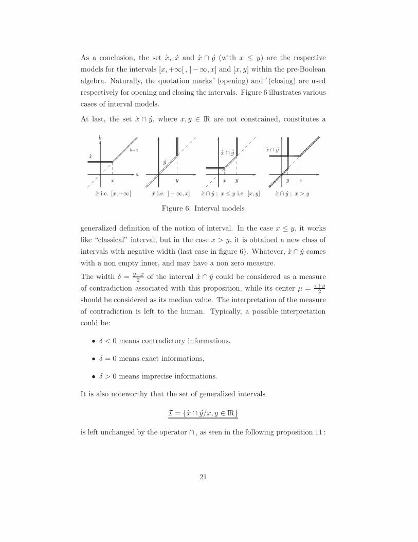
As a conclusion, the set x, x and x ∩ y (with x ≤ y) are the respective

models for the intervals [x,+∞[ , ]−∞, x] and [x, y] within the pre-Boolean

algebra. Naturally, the quotation marks`(opening) and´(closing) are used

respectively for opening and closing the intervals. Figure 6 illustrates various

cases of interval models.

At last, the set x ∩ y, where x, y ∈ IR are not constrained, constitutes a

a

b

b=a

x

x

//

OO

y

y

//

OO

x y

x ∩ y

//

OO

y x

x ∩ y

//

OO

x i.e. [x,+∞[ x i.e. ] −∞, x] x ∩ y ; x ≤ y i.e. [x, y] x ∩ y ; x > y

Figure 6: Interval models

generalized definition of the notion of interval. In the case x ≤ y, it works

like “classical” interval, but in the case x > y, it is obtained a new class of

intervals with negative width (last case in figure 6). Whatever, x∩ y comes

with a non empty inner, and may have a non zero measure.

The width δ = y−x2 of the interval x ∩ y could be considered as a measure

of contradiction associated with this proposition, while its center µ = x+y2

should be considered as its median value. The interpretation of the measure

of contradiction is left to the human. Typically, a possible interpretation

could be:

• δ < 0 means contradictory informations,

• δ = 0 means exact informations,

• δ > 0 means imprecise informations.

It is also noteworthy that the set of generalized intervals

I = x ∩ y/x, y ∈ IR

is left unchanged by the operator ∩ , as seen in the following proposition 11 :

21

Proposition 11 (Stability) Let x1, x2, y1, y2 ∈ IR .

Define x = maxx1, x2 and y = miny1, y2 .

Then (x1 ∩ y1) ∩ (x2 ∩ y2) = x ∩ y .

Proof is obvious.

This last property make possible the definition of basic belief assignment

over generalized intervals only. This assumption is clearly necessary in or-

der to reduce the complexity of the evidence modelling. Behind this as-

sumption is the idea that a continuous measure is described by an impre-

cision/contradiction around the measured value. Such hypothesis has been

made by Smets and Ristic[6]. From now on, all the defined bba will be

zeroed outside I. Now, since I is invariant by ∩ , it is implied that all the

bba which will be manipulated, from sensors or after fusion, will be zeroed

outside I. This makes the basic belief assignments equivalent to a density

over the 2-dimension space IR2 .

4.2 Definition and manipulation of the belief

The definitions of bba, belief and fusion result directly from section 2, but

of course the bba becomes density and the summations are replaced by

integrations.

Basic Belief Assignment. As discussed previously, it is hypothesized

that the measures are characterized by a precision interval around the mea-

sured values. In addition, there is an uncertainty about the measure which

is translated into a basic belief assignment over the precision intervals.

According to these hypotheses, a bba will be a non negatively valued func-

tion m defined over U , zeroed outside I (set of generalized intervals), and

such that:∫

x,y∈IRm(x ∩ y)dxdy = 1 .

Belief function. The function of belief, Bel, is defined for any measurable

proposition φ ∈ U by:

Bel (φ) =

∫

x∩y⊂φm(x ∩ y)dxdy .

22

In particular, for a generalized interval x ∩ y :

Bel (x ∩ y) =

∫ +∞

u=x

∫ y

v=−∞m(u ∩ v)dudv .

Fusion rule. Being given two basic belief assignments m1 and m2, the

fused basic belief assignment m1 ⊕m2 is defined by the curviline integral:

m1 ⊕m2(x ∩ y) =

∫

C=(φ,ψ)/φ∩ψ=x∩ym1(φ)m2(ψ) dC .

Now, from hypothesis it is assumed that mi is positive only for intervals of

the form xi ∩ yi. Proposition 11 implies:

x1 ∩ y1 ∩ x2 ∩ y2 = x ∩ y where

x = maxx1, x2 ,

y = miny1, y2 .

It is then deduced:

m1 ⊕m2(x ∩ y) =

∫ x

x2=−∞

∫ +∞

y2=ym1(x ∩ y)m2(x2 ∩ y2)dx2dy2

+

∫ x

x1=−∞

∫ +∞

y1=ym1(x1 ∩ y1)m2(x ∩ y)dx1dy1

+

∫ x

x1=−∞

∫ +∞

y2=ym1(x1 ∩ y)m2(x ∩ y2)dx1dy2

+

∫ x

x2=−∞

∫ +∞

y1=ym1(x ∩ y1)m2(x2 ∩ y)dx2dy1 .

In particular, it is now justified that a bba, from sensors or fused, will always

be zeroed outside I .

5 Implementation of the continuous model

Setting. In this implementation, the study has been restricted to the

interval [−1, 1] instead of IR. The previous results still hold by trunc-

tating over [−1, 1] . In particular, any bba m is zeroed outside I1−1 =

x ∩ y/x, y ∈ [−1, 1] and its related belief function is defined by:

Bel (x ∩ y) =

∫ 1

u=x

∫ y

v=−1m(u ∩ v)dudv ,

23

for any generalized interval of I1−1 . The bba resulting of the fusion of two

bbas m1 and m2 is defined by:

m1 ⊕m2(x ∩ y) =

∫ x

x2=−1

∫ 1

y2=ym1(x ∩ y)m2(x2 ∩ y2)dx2dy2

+

∫ x

x1=−1

∫ 1

y1=ym1(x1 ∩ y1)m2(x ∩ y)dx1dy1

+

∫ x

x1=−1

∫ 1

y2=ym1(x1 ∩ y)m2(x ∩ y2)dx1dy2

+

∫ x

x2=−1

∫ 1

y1=ym1(x ∩ y1)m2(x2 ∩ y)dx2dy1 .

Method. A theorical computation of these integrals seems uneasy. An ap-

proximation of the densities and of the integrals has been considered. More

precisely, the densities have been approximitated by means of 2-dimension

Chebyshev polynomials , which have several good properties:

• The approximation grows quickly with the degree of the polynomial,

without oscilliation phenomena,

• The Chebyshev transform is quite related to the fourier transform,

which makes the parameters of the polynoms really quickly computable

by means of a Fast Fourier Transform,

• Integration is easy to compute.

In our tests, we have chosen a Chebyshev approximation of degree 128×128 ,

which is more than sufficient for an almost exact computation.

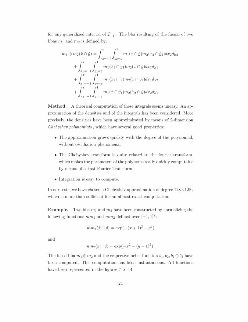
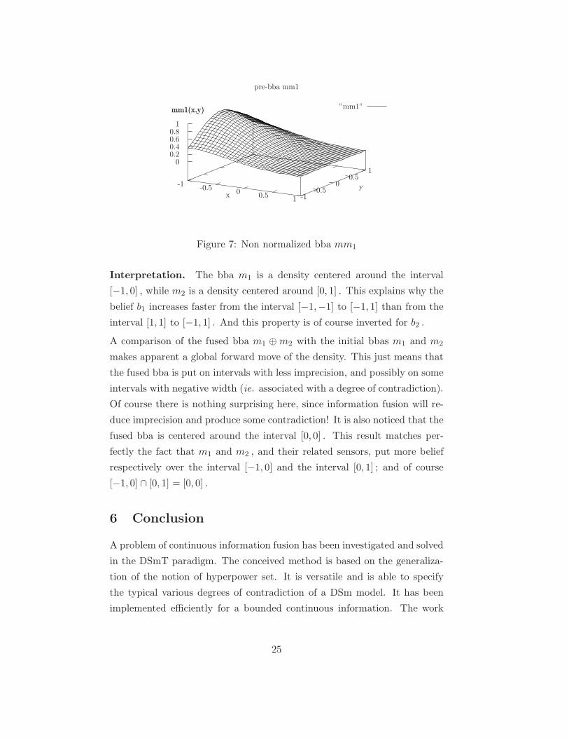
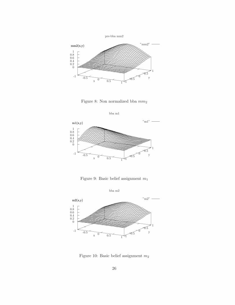
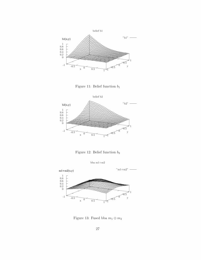
Example. Two bba m1 and m2 have been constructed by normalizing the

following functions mm1 and mm2 defined over [−1, 1]2 :

mm1(x ∩ y) = exp(−(x+ 1)2 − y2)

and

mm2(x ∩ y) = exp(−x2 − (y − 1)2) .

The fused bba m1 ⊕m2 and the respective belief function b1, b2, b1 ⊕ b2 have

been computed. This computation has been instantaneous. All functions

have been represented in the figures 7 to 14.

24

-1 -0.5 0 0.5 1 -1-0.5

00.5

10

0.20.40.60.8

1

mm1(x,y)

pre-bba mm1

”mm1”

xy

mm1(x,y)

Figure 7: Non normalized bba mm1

Interpretation. The bba m1 is a density centered around the interval

[−1, 0] , while m2 is a density centered around [0, 1] . This explains why the

belief b1 increases faster from the interval [−1,−1] to [−1, 1] than from the

interval [1, 1] to [−1, 1] . And this property is of course inverted for b2 .

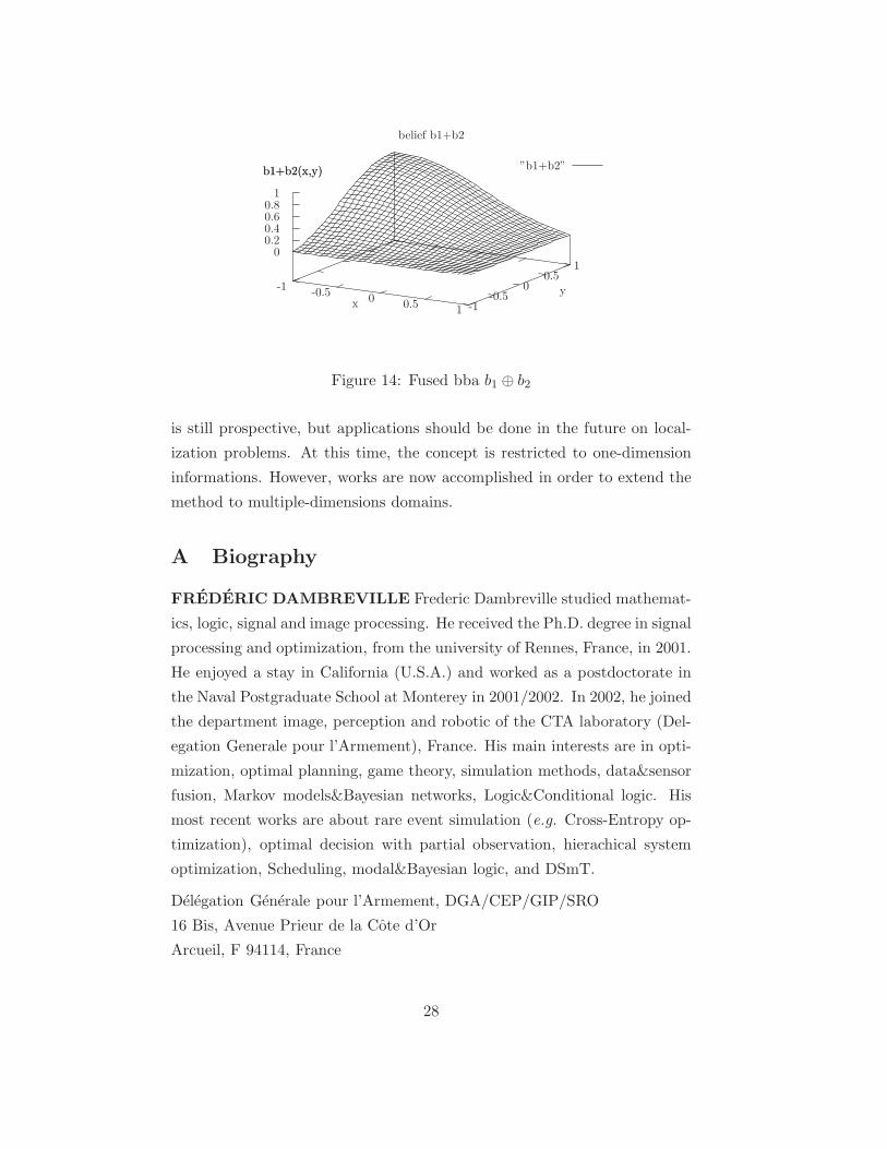
A comparison of the fused bba m1 ⊕m2 with the initial bbas m1 and m2

makes apparent a global forward move of the density. This just means that

the fused bba is put on intervals with less imprecision, and possibly on some

intervals with negative width (ie. associated with a degree of contradiction).

Of course there is nothing surprising here, since information fusion will re-

duce imprecision and produce some contradiction! It is also noticed that the

fused bba is centered around the interval [0, 0] . This result matches per-

fectly the fact that m1 and m2 , and their related sensors, put more belief

respectively over the interval [−1, 0] and the interval [0, 1] ; and of course

[−1, 0] ∩ [0, 1] = [0, 0] .

6 Conclusion

A problem of continuous information fusion has been investigated and solved

in the DSmT paradigm. The conceived method is based on the generaliza-

tion of the notion of hyperpower set. It is versatile and is able to specify

the typical various degrees of contradiction of a DSm model. It has been

implemented efficiently for a bounded continuous information. The work

25

-1 -0.5 0 0.5 1 -1-0.5

00.5

10

0.20.40.60.8

1

mm2(x,y)

pre-bba mm2

”mm2”

xy

mm2(x,y)

Figure 8: Non normalized bba mm2

-1 -0.5 0 0.5 1 -1-0.5

00.5

10

0.20.40.60.8

1

m1(x,y)

bba m1

”m1”

xy

m1(x,y)

Figure 9: Basic belief assignment m1

-1 -0.5 0 0.5 1 -1-0.5

00.5

10

0.20.40.60.8

1

m2(x,y)

bba m2

”m2”

xy

m2(x,y)

Figure 10: Basic belief assignment m2

26

-1 -0.5 0 0.5 1 -1-0.5

00.5

10

0.20.40.60.8

1

b1(x,y)

belief b1

”b1”

xy

b1(x,y)

Figure 11: Belief function b1

-1 -0.5 0 0.5 1 -1-0.5

00.5

10

0.20.40.60.8

1

b2(x,y)

belief b2

”b2”

xy

b2(x,y)

Figure 12: Belief function b2

-1 -0.5 0 0.5 1 -1-0.5

00.5

10

0.20.40.60.8

1

m1+m2(x,y)

bba m1+m2

”m1+m2”

xy

m1+m2(x,y)

Figure 13: Fused bba m1 ⊕m2

27

-1 -0.5 0 0.5 1 -1-0.5

00.5

10

0.20.40.60.8

1

b1+b2(x,y)

belief b1+b2

”b1+b2”

xy

b1+b2(x,y)

Figure 14: Fused bba b1 ⊕ b2

is still prospective, but applications should be done in the future on local-

ization problems. At this time, the concept is restricted to one-dimension

informations. However, works are now accomplished in order to extend the

method to multiple-dimensions domains.

A Biography

FREDERIC DAMBREVILLE Frederic Dambreville studied mathemat-

ics, logic, signal and image processing. He received the Ph.D. degree in signal

processing and optimization, from the university of Rennes, France, in 2001.

He enjoyed a stay in California (U.S.A.) and worked as a postdoctorate in

the Naval Postgraduate School at Monterey in 2001/2002. In 2002, he joined

the department image, perception and robotic of the CTA laboratory (Del-

egation Generale pour l’Armement), France. His main interests are in opti-

mization, optimal planning, game theory, simulation methods, data&sensor

fusion, Markov models&Bayesian networks, Logic&Conditional logic. His

most recent works are about rare event simulation (e.g. Cross-Entropy op-

timization), optimal decision with partial observation, hierachical system

optimization, Scheduling, modal&Bayesian logic, and DSmT.

Delegation Generale pour l’Armement, DGA/CEP/GIP/SRO

16 Bis, Avenue Prieur de la Cote d’Or

Arcueil, F 94114, France

28

Web: http://www.FredericDambreville.com

Email: http://email.FredericDambreville.com

References

[1] Boolean algebra topic at the wikipedia.

http://en.wikipedia.org/wiki/Boolean algebra

http://en.wikipedia.org/wiki/Field of sets

[2] F. Smarandache and J. Dezert editors, Advances and Applications of

DSmT for Information Fusion, American Research Press, Rohoboth,

2004.

http://www.gallup.unm.edu/∼smarandache/DSmT.htm

[3] A. Tchamova, J. Dezert, Tz. Semerdjiev, P. Konstanttinova, Target

Tracking with Generalized Data Association based on the General DSm

Rule of Combination, Conference Fusion 2004, Sweden, 2004.

[4] S. Corgne, L. Hubert-Moy, G. Mercier, J. Dezert, Application of DSmT

for Land Cover Change Prediction, in Advances and Applications of

DSmT for Information Fusion, American Research Press, Rohoboth,

2004.

[5] P. Smets and R. Kennes, The transferable belief model, Artificial Intelli-

gence 66, pp 191-234, 1994

[6] B. Ristic and P. Smets, Belief function theory on the continuous space

with an application to model based classification, IPMU 2004, Italy, 2004.

[7] T. M. Strat, Continuous belief functions for evidential reasoning, AAAI

1984, pp 308-313.

[8] A. P. Dempster, Upper and lower probabilities induced by a multiple

valued mapping, Ann. Math. Statistics, no. 38, pp. 325–339, 1967.

[9] Shafer G., A Mathematical Theory of Evidence, Princeton Univ. Press,

Princeton, NJ, 1976.

29