oracle r enterprise 1.3 transparency layer

<Insert Picture Here>

©2012 Oracle – All Rights Reserved

Learning R Series Session 2: Oracle R Enterprise 1.3 Transparency Layer

Mark Hornick, Senior Manager, Development

Oracle Advanced Analytics

2

Learning R Series 2012

Session Title

Session 1 Introduction to Oracle's R Technologies and Oracle R Enterprise 1.3

Session 2 Oracle R Enterprise 1.3 Transparency Layer

Session 3 Oracle R Enterprise 1.3 Embedded R Execution

Session 4 Oracle R Enterprise 1.3 Predictive Analytics

Session 5 Oracle R Enterprise 1.3 Integrating R Results and Images with OBIEE Dashboards

Session 6 Oracle R Connector for Hadoop 2.0 New features and Use Cases

3

The following is intended to outline our general product direction. It

is intended for information purposes only, and may not be

incorporated into any contract. It is not a commitment to deliver

any material, code, or functionality, and should not be relied upon

in making purchasing decisions.

The development, release, and timing of any features or

functionality described for Oracle’s products remain at the sole

discretion of Oracle.

4

Topics

• What does “transparency” mean?

• Connecting to Oracle Database through ORE

• Examples with the Transparency Layer

• ORE 1.3 New Features

– Options for Connecting to Oracle Database

– R Object Persistence in Oracle Database

– Support for Time Series Analysis

– Ordering Framework

– In-database Sampling and Random Partitioning

– Column name length in ore.frame

• Comparing R and ORE for building and scoring with linear models

• HIVE transparency

• Summary


5

What does “transparency” mean?


6

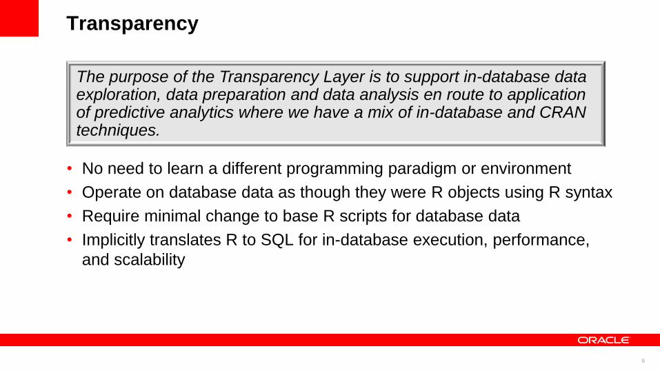
Transparency

• No need to learn a different programming paradigm or environment

• Operate on database data as though they were R objects using R syntax

• Require minimal change to base R scripts for database data

• Implicitly translates R to SQL for in-database execution, performance,

and scalability

The purpose of the Transparency Layer is to support in-database data exploration, data preparation and data analysis en route to application of predictive analytics where we have a mix of in-database and CRAN techniques.

7

Establish a connection using ore.connect

• Function is.ore.connected returns TRUE if you’re already

connected to an Oracle Database

• Function ore.connect parameters

– User id, SID, host, password

– Port defaults to 1521

– “all” set to TRUE loads all tables from the schema into ORE metadata and

makes them available at the R command line as ore.frame objects

• Function ore.ls lists all the available tables by name

if (!is.ore.connected())

ore.connect("rquser", "orcl",

"localhost", "rquser", all=TRUE)

ore.ls()

8

Manipulating Data

• Column selection df <- ONTIME_S[,c("YEAR","DEST","ARRDELAY")]

class(df)

head(df)

head(ONTIME_S[,c(1,4,23)])

head(ONTIME_S[,-(1:22)])

• Row selection df1 <- df[df$DEST=="SFO",]

class(df1)

df2 <- df[df$DEST=="SFO",c(1,3)]

df3 <- df[df$DEST=="SFO" | df$DEST=="BOS",1:3]

head(df1)

head(df2)

head(df3)


9

Manipulating Data – SQL equivalent

R

• Column selection df <- ONTIME_S[,c("YEAR","DEST","ARRDELAY")]

head(df)

head(ONTIME_S[,c(1,4,23)])

head(ONTIME_S[,-(1:22)])

• Row selection df1 <- df[df$DEST=="SFO",]

df2 <- df[df$DEST=="SFO",c(1,3)]

df3 <- df[df$DEST=="SFO" | df$DEST=="BOS",1:3]

SQL

• Column selection create view df as

select YEAR, DEST, ARRDELAY

from ONTIME_S;

-- cannot do next two, e.g., by number & exclusion

• Row selection create view df1 as

select * from df where DEST=‘SFO’;

create view df2 as

select YEAR, ARRDELAY from df where DEST=‘SFO’

create view df3 as

select YEAR, DEST, ARRDELAY from df

where DEST=‘SFO’ or DEST=‘BOS’


Benefits of R:

Deferred execution

Incremental query refinement

10

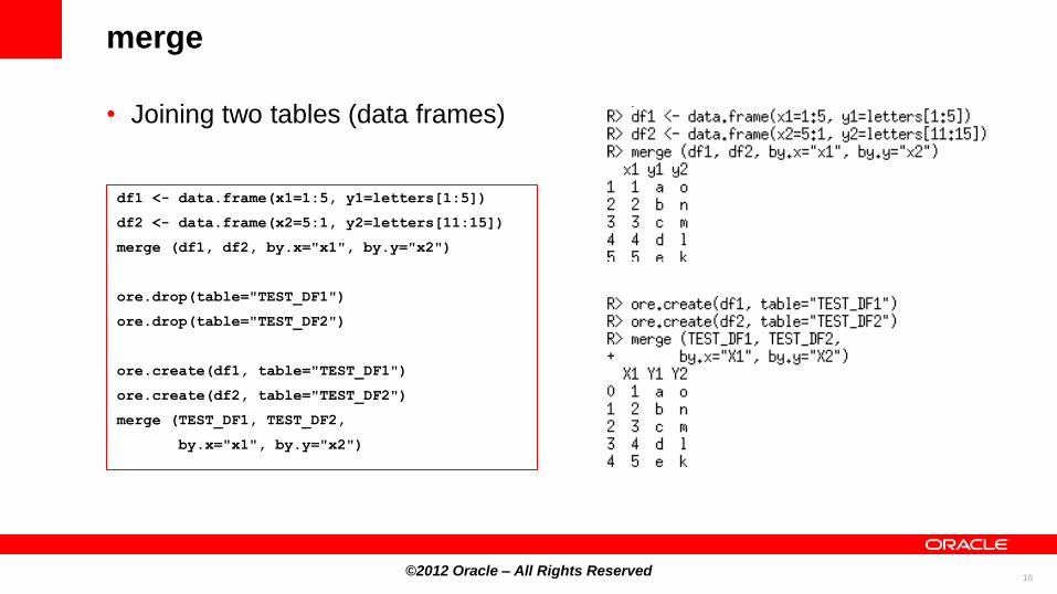
merge

• Joining two tables (data frames)


df1 <- data.frame(x1=1:5, y1=letters[1:5])

df2 <- data.frame(x2=5:1, y2=letters[11:15])

merge (df1, df2, by.x="x1", by.y="x2")

ore.drop(table="TEST_DF1")

ore.drop(table="TEST_DF2")

ore.create(df1, table="TEST_DF1")

ore.create(df2, table="TEST_DF2")

merge (TEST_DF1, TEST_DF2,

by.x="x1", by.y="x2")

11

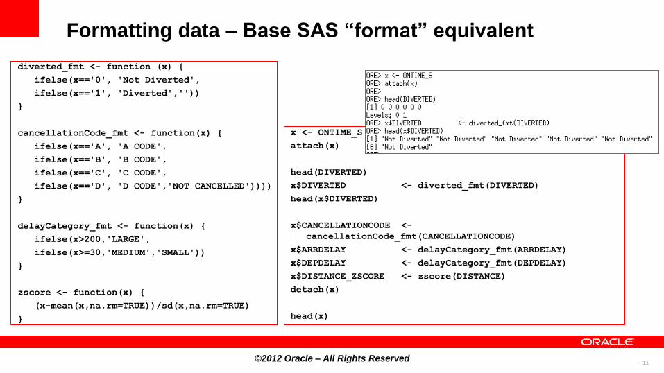
Formatting data – Base SAS “format” equivalent

diverted_fmt <- function (x) {

ifelse(x=='0', 'Not Diverted',

ifelse(x=='1', 'Diverted',''))

}

cancellationCode_fmt <- function(x) {

ifelse(x=='A', 'A CODE',

ifelse(x=='B', 'B CODE',

ifelse(x=='C', 'C CODE',

ifelse(x=='D', 'D CODE','NOT CANCELLED'))))

}

delayCategory_fmt <- function(x) {

ifelse(x>200,'LARGE',

ifelse(x>=30,'MEDIUM','SMALL'))

}

zscore <- function(x) {

(x-mean(x,na.rm=TRUE))/sd(x,na.rm=TRUE)

}

x <- ONTIME_S

attach(x)

head(DIVERTED)

x$DIVERTED <- diverted_fmt(DIVERTED)

head(x$DIVERTED)

x$CANCELLATIONCODE <-

cancellationCode_fmt(CANCELLATIONCODE)

x$ARRDELAY <- delayCategory_fmt(ARRDELAY)

x$DEPDELAY <- delayCategory_fmt(DEPDELAY)

x$DISTANCE_ZSCORE <- zscore(DISTANCE)

detach(x)

head(x)


12

Formatting data or alternatively, using transform ( )

ONTIME_S <- transform(ONTIME_S,

DIVERTED = ifelse(DIVERTED == 0, 'Not Diverted',

ifelse(DIVERTED == 1, 'Diverted', '')),

CANCELLATIONCODE =

ifelse(CANCELLATIONCODE == 'A', 'A CODE',

ifelse(CANCELLATIONCODE == 'B', 'B CODE',

ifelse(CANCELLATIONCODE == 'C', 'C CODE',

ifelse(CANCELLATIONCODE == 'D', 'D CODE', 'NOT CANCELLED')))),

ARRDELAY = ifelse(ARRDELAY > 200, 'LARGE',

ifelse(ARRDELAY >= 30, 'MEDIUM', 'SMALL')),

DEPDELAY = ifelse(DEPDELAY > 200, 'LARGE',

ifelse(DEPDELAY >= 30, 'MEDIUM', 'SMALL')),

DISTANCE_ZSCORE =(DISTANCE - mean(DISTANCE, na.rm=TRUE))/sd(DISTANCE, na.rm=TRUE))


13

ORE Packages

Package Description

ORE Top Level Package for Oracle R Enterprise

OREbase Corresponds to R’s base package

OREstats Corresponds to R’s stat package

OREgraphics Corresponds to R’s graphics package

OREeda Exploratory data analysis package containing

Base SAS PROC-equivalent functionality

OREdm Exposes Oracle Data Mining algorithms

OREpredict Enables scoring data in Oracle DB using R models

ORExml Supports XML translation between R and

Oracle Database


Transparency Layer

14

Options for Connecting to Oracle Database


15

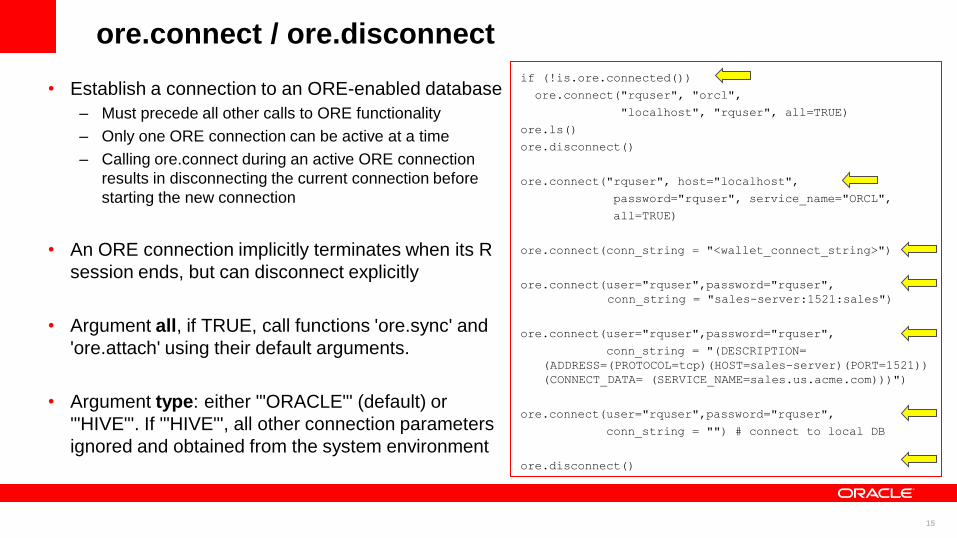
ore.connect / ore.disconnect

• Establish a connection to an ORE-enabled database

– Must precede all other calls to ORE functionality

– Only one ORE connection can be active at a time

– Calling ore.connect during an active ORE connection

results in disconnecting the current connection before

starting the new connection

• An ORE connection implicitly terminates when its R

session ends, but can disconnect explicitly

• Argument all, if TRUE, call functions 'ore.sync' and

'ore.attach' using their default arguments.

• Argument type: either '"ORACLE"' (default) or

'"HIVE"'. If '"HIVE"', all other connection parameters

ignored and obtained from the system environment

if (!is.ore.connected())

ore.connect("rquser", "orcl",

"localhost", "rquser", all=TRUE)

ore.ls()

ore.disconnect()

ore.connect("rquser", host="localhost",

password="rquser", service_name="ORCL",

all=TRUE)

ore.connect(conn_string = "<wallet_connect_string>")

ore.connect(user="rquser",password="rquser",

conn_string = "sales-server:1521:sales")


conn_string = "(DESCRIPTION=

(ADDRESS=(PROTOCOL=tcp)(HOST=sales-server)(PORT=1521))

(CONNECT_DATA= (SERVICE_NAME=sales.us.acme.com)))")


conn_string = "") # connect to local DB

ore.disconnect()

16

ORE functions for interacting with database data

v <- ore.push(c(1,2,3,4,5))

df <- ore.push(data.frame(a=1:5, b=2:6))

ore.sync()

ore.sync("RQUSER")

ore.sync(table=c("ONTIME_S", "NARROW"))

ore.sync("RQUSER", table=c("ONTIME_S", "NARROW"))

ore.exists("ONTIME_S", "RQUSER")

Store R object in database as temporary object, returns handle to object. Data frame, matrix, and vector to table, list/model/others to serialized object

Synchronize ORE proxy objects in R with tables/views available in database, on a per schema basis

Returns TRUE if named table or view exists in schema


Caveat for ore.sync:

Data types long, long raw, UDTs, and reference types not supported

When encountered, warning issued and table not available, e.g., via ore.ls()

17

ORE functions for interacting with database data

ore.ls()

ore.ls("RQUSER")

ore.ls("RQUSER",all.names=TRUE)

ore.ls("RQUSER",all.names=TRUE, pattern= "NAR")

t <- ore.get("ONTIME_S","RQUSER")

ore.attach("RQUSER")

ore.attach("RQUSER", pos=2)

ore.detach("RQUSER")

ore.rm("DF1")

ore.rm(list("TABLE1","TABLE2"), "RQUSER")

ore.exec("create table F2 as select * from ONTIME_S")

List the objects available in ORE environment mapped to database schema.

All.names=FALSE excludes names starting with a ‘.’

Obtain object to named table/view in schema.

Make database objects visible in R for named schema. Can place corresponding environment in specific position in env path.

Remove schema’s environment from the object search path.

Remove table or view from schema’s R environment.


Execute SQL or PL/SQL without return value

18

R Object Persistence in Oracle Database


19

R Object Persistence What does R provide?

• save()

• load()

• Serialize and unserialize R objects to files

• Standard R functions to persist R objects

do not interoperate with Oracle Database

• Use cases include

– Persist models for subsequent data scoring

– Save entire R state to reload next R session

Filesystem

load("myRObjects.RData")

ls()

“x1” “x2”

“myRObjs.RData"

x1 <- lm(...)

x2 <- data.frame(...)

save(x1,x2,file="myRObjects.RData")

20

R Object Persistence with ORE

• ore.save()

• ore.load()

• Provide database storage to save/restore

R and ORE objects across R sessions

• Use cases include

– Enable passing of predictive model for embedded R

execution, instead of recreating them inside the R

functions

– Passing arguments to R functions with

embedded R execution

– Preserve ORE objects across R sessions

x1 <- ore.lm(...)

x2 <- ore.frame(...)

ore.save(x1,x2,name="ds1")

R Datastore

ore.load(name="ds1")

ls()

“x1” “x2”

ds1 {x1,x2}

21

Datastore Details

• Each schema has its own datastore table where R objects are

saved as named datastores

• Maintain referential integrity of saved objects

– Account for object auto-deleted at end of session

– Database objects, such as tables, ODM models, etc., not used by any

saved R object deleted when R session ends

• Functions

– ore.save, ore.load

– ore.datastore, ore.datastoreSummary

– ore.delete

22

ore.save

DAT1 <- ore.push(ONTIME_S[,c("ARRDELAY", "DEPDELAY", "DISTANCE")])

ore.lm.mod <- ore.lm(ARRDELAY ~ DISTANCE + DEPDELAY, DAT1 )

lm.mod <- lm(mpg ~ cyl + disp + hp + wt + gear, mtcars)

nb.mod <- ore.odmNB(YEAR ~ ARRDELAY + DEPDELAY + log(DISTANCE), ONTIME_S)

ore.save(ore.lm.mod, lm.mod, nb.mod, name = "myModels")

• R objects and their referenced data tables are saved into the datastore of the connected schema

• Saved R objects are identified with datastore name myModels

• Arguments

– ... the names of the objects to be saved (as symbols or character strings)

– list — a character vector containing the names of objects to be saved

– name — datastore name to identify the set of saved R objects in current user's schema

– envir — environment to search for objects to be saved

– overwrite — boolean indicating whether to overwrite the existing named datastore

– append — boolean indicating whether to append to the named datastore

– description -- comments about the datastore

23

ore.load

ore.load(name = "myModels")

• Accesses the R objects stored in the connected schema with datastore name

"myModels"

• These are restored to the R .GlobalEnv environment

• Objects ore.lm.mod, lm.mod, nb.mod can now be referenced and used

• Arguments

– name — datastore name under current user schema in the connected schema

– list — a character vector containing the names of objects to be loaded from the datastore,

default is all objects

– envir — the environment where R objects should be loaded in R

24

ore.datastore

dsinfo <- ore.datastore(pattern = "my*")

• List basic information about R datastore in connected schema

• Result dsinfo is a data.frame

– Columns:

datastore.name, object.count (# objects in datastore), size (in bytes), creation.date, description

– Rows: one per datastore object in schema

• Arguments – one of the following

– name — name of datastore under current user schema from which to return data

– pattern — optional regular expression. Only the datastores whose names match the pattern are

returned. By default, all the R datastores under the schema are returned

25

ore.datastore example

26

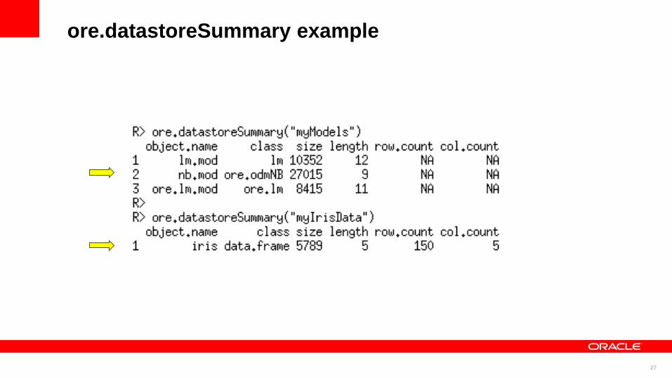
ore.datastoreSummary

objinfo <- ore.datastoreSummary(name = "myModels")

• List names of R objects that are saved within named datastore in connected schema

• Result objinfo is a data.frame

– Columns:

object.name, class, size (in bytes), length (if vector),

row.count (if data,frame), col.count (if data.frame)

– Rows: one per datastore object in schema

• Argument

– name — name of datastore under current user schema from which to list object contents

27

ore.datastoreSummary example

28

ore.delete

ore.delete(name = "myModels")

• Deletes the named datastore in connected schema and its corresponding objects

• If objects saved in other datastores referenced the same objects, referenced objects

are only cleaned up when there are no more references

• Argument

– name — name of datastore under current user schema from which to return data

29

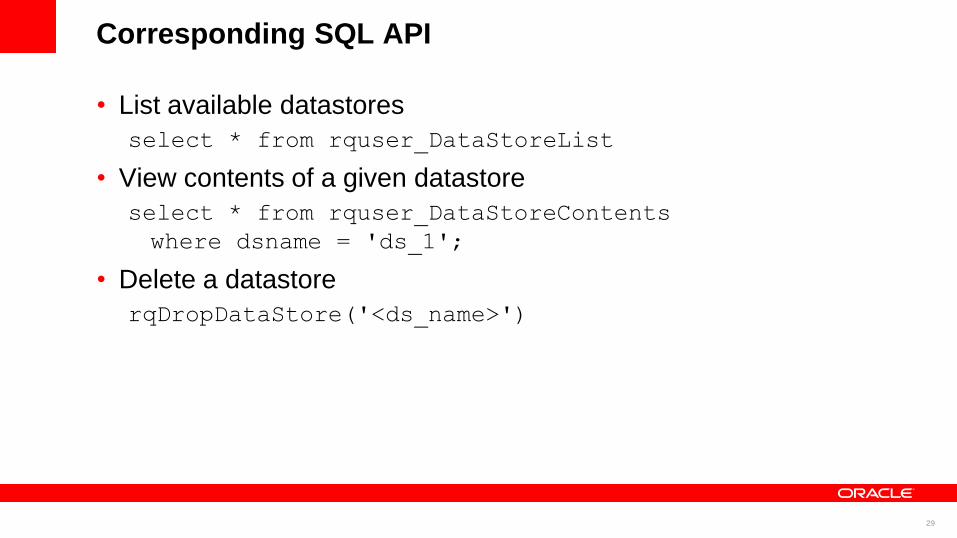
Corresponding SQL API

• List available datastores

select * from rquser_DataStoreList

• View contents of a given datastore

select * from rquser_DataStoreContents

where dsname = 'ds_1';

• Delete a datastore

rqDropDataStore('<ds_name>')

30

Using datastore objects in embedded R SQL API

begin

-- sys.rqScriptDrop('buildmodel_1');

sys.rqScriptCreate('buildmodel_1',

'function(dat, out.dsname, out.objname) {

assign(out.objname, lm(ARRDELAY ~ DISTANCE + DEPDELAY, dat, model = FALSE))

ore.save(list=out.objname, name = out.dsname, overwrite=TRUE)

cbind(dsname=out.dsname, ore.datastoreSummary(name= out.dsname))

}');

end;

/

-- build model

select * from table(rqTableEval(

cursor(select ARRDELAY, DISTANCE, DEPDELAY from ONTIME_S),

cursor(select 'ontime_model' as "out.dsname",'lm.mod' as "out.objname",

1 as "ore.connect" from dual),

'select * from rquser_datastoreContents',

'buildmodel_1'));

1

2

3

4

5

6

7

8

9

10

11

12

13

14

15

16

17

18

31

Support for Time Series Analytics


32

Time Series Analysis Motivation

• Time series data is widely prevalent

– Stock / trading data

– Sales data

– Employment data

• Need to understand trends,

seasonable effects, residuals

33

Time Series Analysis

• Aggregation and

moving window analysis

of large time series data

• Equivalent functionality

from popular R

packages for data

preparation available

in-database

…

34

Support for Time Series Data

• Support for Oracle data types – DATE, TIMESTAMP

– TIMESTAMP WITH TIME ZONE

– TIMESTAMP WITH LOCAL TIME ZONE

• Analytic capabilities

– Date arithmetic, Aggregations & Percentiles

– Moving window calculations:

ore.rollmax ore.rollmean ore.rollmin ore.rollsd

ore.rollsum ore.rollvar, ore.rollsd

35

Date and Time Motivation

• Support for key data types in Oracle Database and R

• Date and time handling essential for time series data

• Date and time representation unified in Oracle Database, but

R lacks a standard structure and functions

– E.g., Date, POSIXct, POSIXlt, difftime in R base package

– Mapping data types important for transparent database access

36

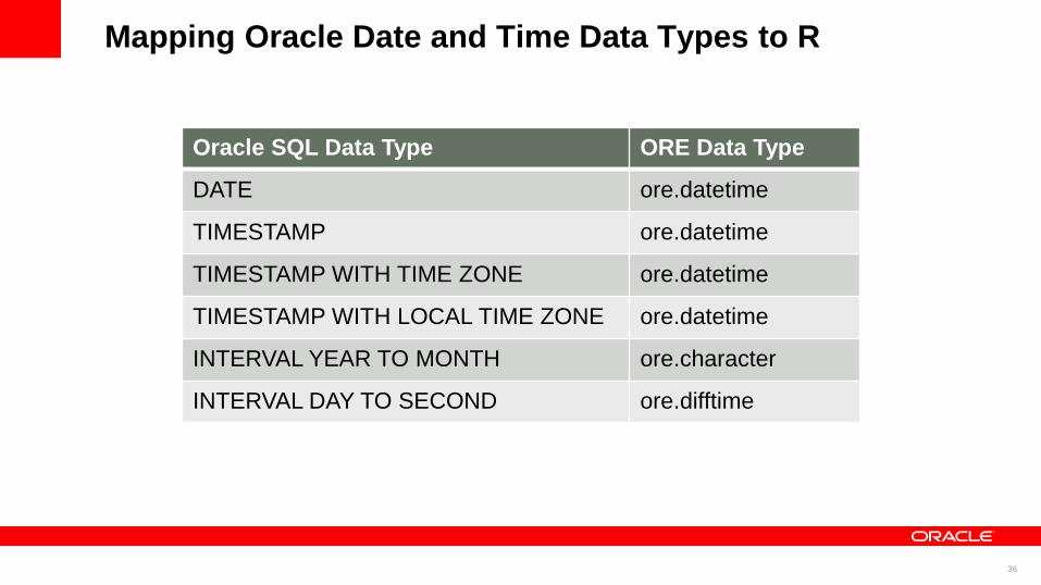
Mapping Oracle Date and Time Data Types to R

Oracle SQL Data Type ORE Data Type

DATE ore.datetime

TIMESTAMP ore.datetime

TIMESTAMP WITH TIME ZONE ore.datetime

TIMESTAMP WITH LOCAL TIME ZONE ore.datetime

INTERVAL YEAR TO MONTH ore.character

INTERVAL DAY TO SECOND ore.difftime

37

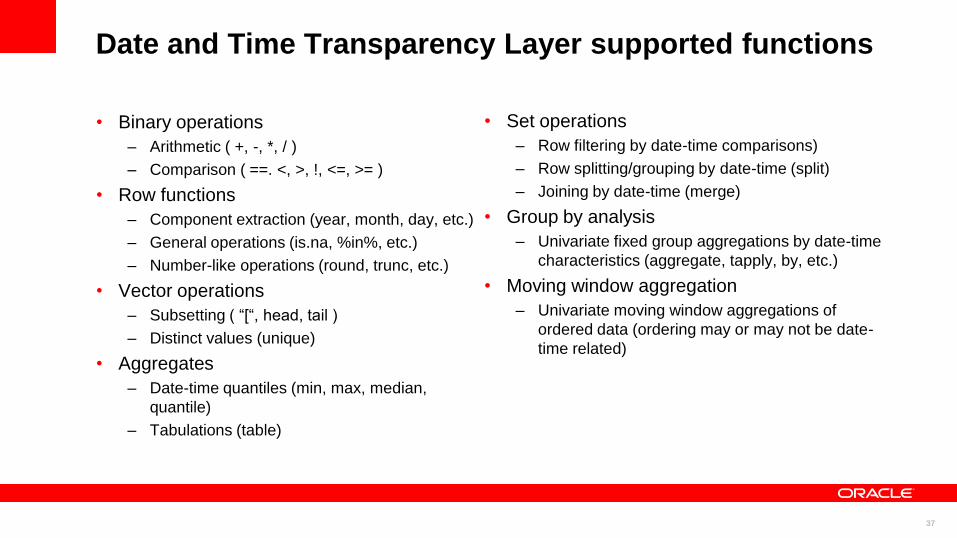
Date and Time Transparency Layer supported functions

• Binary operations

– Arithmetic ( +, -, *, / )

– Comparison ( ==. <, >, !, <=, >= )

• Row functions

– Component extraction (year, month, day, etc.)

– General operations (is.na, %in%, etc.)

– Number-like operations (round, trunc, etc.)

• Vector operations

– Subsetting ( “[“, head, tail )

– Distinct values (unique)

• Aggregates

– Date-time quantiles (min, max, median,

quantile)

– Tabulations (table)

• Set operations

– Row filtering by date-time comparisons)

– Row splitting/grouping by date-time (split)

– Joining by date-time (merge)

• Group by analysis

– Univariate fixed group aggregations by date-time

characteristics (aggregate, tapply, by, etc.)

• Moving window aggregation

– Univariate moving window aggregations of

ordered data (ordering may or may not be date-

time related)

38

Date and Time aggregates

N <- 500

mydata <- data.frame(datetime =

seq(as.POSIXct("2001/01/01"),

as.POSIXct("2001/12/31"),

length.out = N),

difftime = as.difftime(runif(N),

units = "mins"),

x = rnorm(N))

MYDATA <- ore.push(mydata)

class(MYDATA)

class(MYDATA$datetime)

head(MYDATA,3)

39

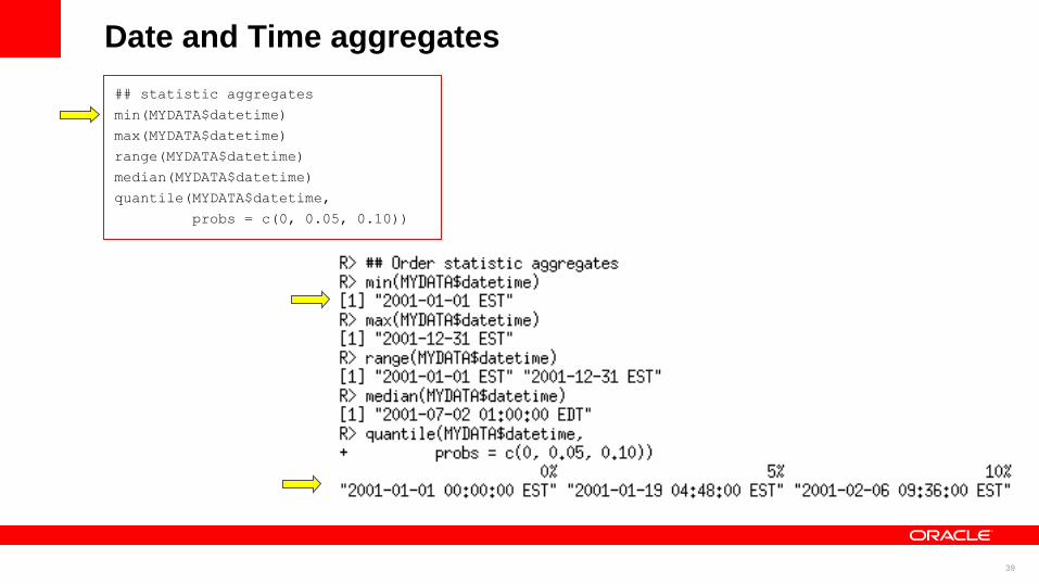
Date and Time aggregates

## statistic aggregates

min(MYDATA$datetime)

max(MYDATA$datetime)

range(MYDATA$datetime)

median(MYDATA$datetime)

quantile(MYDATA$datetime,

probs = c(0, 0.05, 0.10))

40

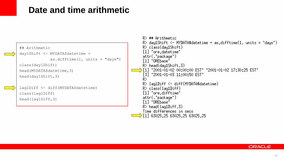
Date and time arithmetic

## Arithmetic

day1Shift <- MYDATA$datetime +

as.difftime(1, units = "days")

class(day1Shift)

head(MYDATA$datetime,3)

head(day1Shift,3)

lag1Diff <- diff(MYDATA$datetime)

class(lag1Diff)

head(lag1Diff,3)

41

Date and time comparisons

isQ1 <- MYDATA$datetime < as.Date("2001/04/01")

class(isQ1)

head(isQ1,3)

isMarch <- isQ1 & MYDATA$datetime >

as.Date("2001/03/01")

class(isMarch)

head(isMarch,3)

sum(isMarch)

eoySubset <- MYDATA[MYDATA$datetime >

as.Date("2001/12/27"), ]

class(eoySubset)

head(eoySubset,3)

42

Date/time accessors

## Date/time accessors

year <- ore.year(MYDATA$datetime)

unique(year)

month <- ore.month(MYDATA$datetime)

range(month)

dayOfMonth <- ore.mday(MYDATA$datetime)

range(dayOfMonth)

hour <- ore.hour(MYDATA$datetime)

range(hour)

minute <- ore.minute(MYDATA$datetime)

range(minute)

second <- ore.second(MYDATA$datetime)

range(second)

43

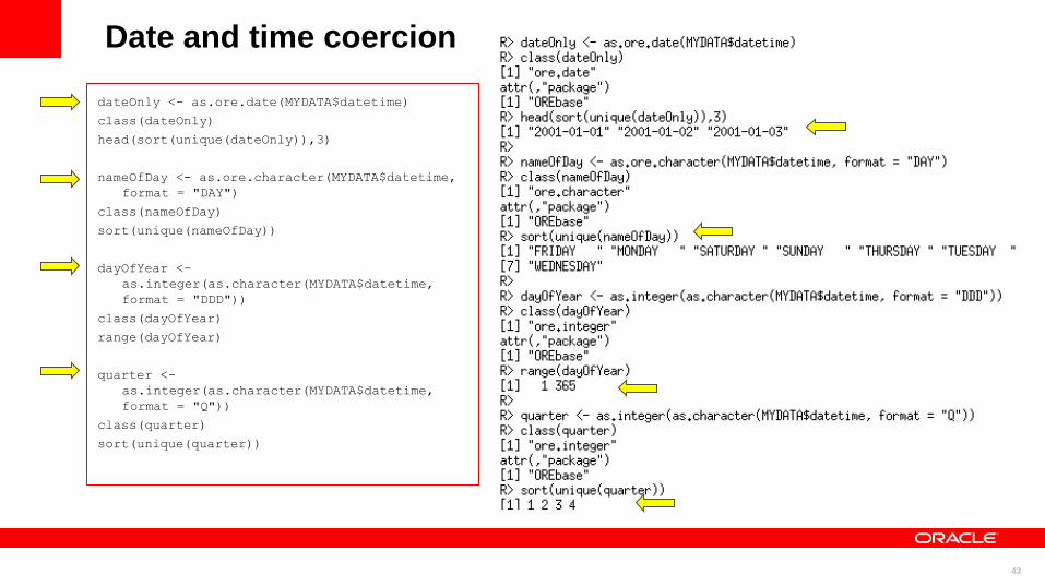
Date and time coercion

dateOnly <- as.ore.date(MYDATA$datetime)

class(dateOnly)

head(sort(unique(dateOnly)),3)

nameOfDay <- as.ore.character(MYDATA$datetime,

format = "DAY")

class(nameOfDay)

sort(unique(nameOfDay))

dayOfYear <-

as.integer(as.character(MYDATA$datetime,

format = "DDD"))

class(dayOfYear)

range(dayOfYear)

quarter <-

as.integer(as.character(MYDATA$datetime,

format = "Q"))

class(quarter)

sort(unique(quarter))

44

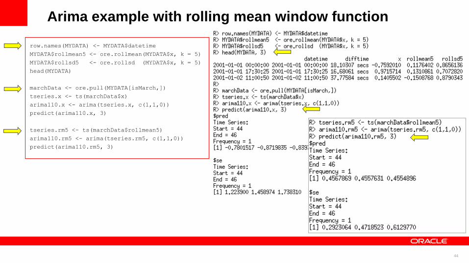
Arima example with rolling mean window function

row.names(MYDATA) <- MYDATA$datetime

MYDATA$rollmean5 <- ore.rollmean(MYDATA$x, k = 5)

MYDATA$rollsd5 <- ore.rollsd (MYDATA$x, k = 5)

head(MYDATA)

marchData <- ore.pull(MYDATA[isMarch,])

tseries.x <- ts(marchData$x)

arima110.x <- arima(tseries.x, c(1,1,0))

predict(arima110.x, 3)

tseries.rm5 <- ts(marchData$rollmean5)

arima110.rm5 <- arima(tseries.rm5, c(1,1,0))

predict(arima110.rm5, 3)

45

Ordering Framework


46

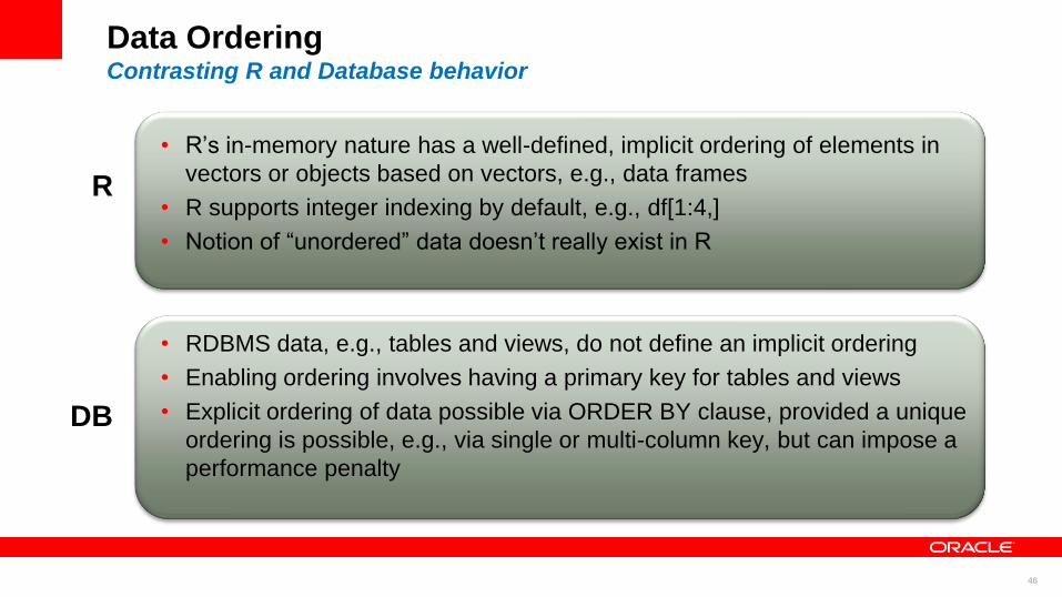
Data Ordering Contrasting R and Database behavior

• R’s in-memory nature has a well-defined, implicit ordering of elements in

vectors or objects based on vectors, e.g., data frames

• R supports integer indexing by default, e.g., df[1:4,]

• Notion of “unordered” data doesn’t really exist in R

• RDBMS data, e.g., tables and views, do not define an implicit ordering

• Enabling ordering involves having a primary key for tables and views

• Explicit ordering of data possible via ORDER BY clause, provided a unique

ordering is possible, e.g., via single or multi-column key, but can impose a

performance penalty

R

DB

47

Ordered and unordered ore.frames

• An ore.frame is ordered if…

– A primary key is defined on the underlying table

– It is produced by certain functions, e.g., “aggregate” and “cbind”

– The row names of the ore.frame are set to unique values

– All input ore.frames to relevant ORE functions are ordered

• An ore.frame is unordered if…

– No primary key is defined on the underlying table

– Even with a primary key is specified, ore.sync parameter use.keys is set to FALSE

– No row names are specified for the ore.frame

– Row names have been set to NULL

– One or more input ore.frames to relevant ORE functions are unordered

48

Ordering Framework: Prepare and view the data

# R

library(kernlab)

data(spam)

s <- spam

s$TS <-as.integer(1:nrow(s)+1000)

s$USERID <- rep(1:50+350, each=2, len=nrow(s))

ore.drop(table='SPAM_PK')

ore.drop(table='SPAM_NOPK')

ore.create(s[,c(59:60,1:28)], table='SPAM_PK')

ore.create(s[,c(59:60,1:28)], table='SPAM_NOPK')

--SQL

alter table SPAM_PK

add constraint SPAM_PK primary key ("USERID","TS");

# R

head(SPAM_PK[,1:8])

head(SPAM_NOPK[,1:8])

49

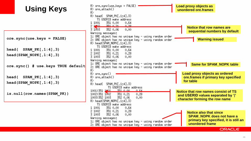
Using Keys

ore.sync(use.keys = FALSE)

head( SPAM_PK[,1:4],3)

head(SPAM_NOPK[,1:4],3)

ore.sync() # use.keys TRUE default

head( SPAM_PK[,1:4],3)

head(SPAM_NOPK[,1:4],3)

is.null(row.names(SPAM_PK))

Load proxy objects as unordered ore.frames

Notice that row names are sequential numbers by default

Warning issued

Same for SPAM_NOPK table

Load proxy objects as ordered ore.frames if primary key specified for table

Notice that row names consist of TS and USERID values separated by ‘|’ character forming the row name

Notice also that since SPAM_NOPK does not have a primary key specified, it is still an unordered frame

50

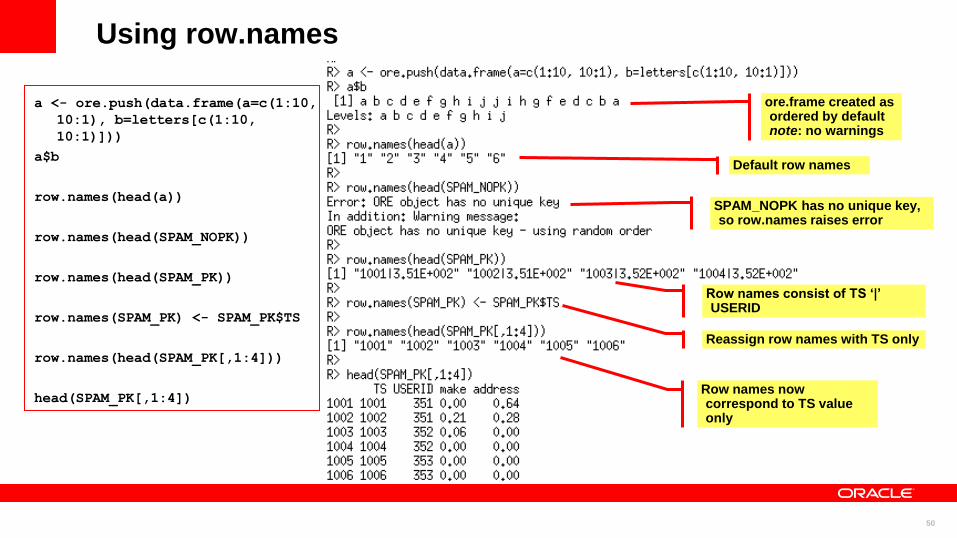
Using row.names

a <- ore.push(data.frame(a=c(1:10,

10:1), b=letters[c(1:10,

10:1)]))

a$b

row.names(head(a))

row.names(head(SPAM_NOPK))

row.names(head(SPAM_PK))

row.names(SPAM_PK) <- SPAM_PK$TS

row.names(head(SPAM_PK[,1:4]))

head(SPAM_PK[,1:4])

ore.frame created as ordered by default note: no warnings

Default row names

SPAM_NOPK has no unique key, so row.names raises error

Row names now correspond to TS value only

Row names consist of TS ‘|’ USERID

Reassign row names with TS only

51

Indexing ore.frames

SPAM_PK["2060", 1:4]

SPAM_PK[as.character(2060:2064), 1:4]

SPAM_PK[2060:2063, 1:4]

Index to a range of rows by row names

Index to a specifically named row

Index to a range of rows by integer index

52

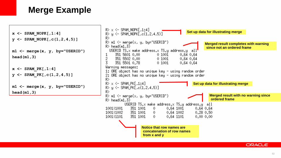
Merge Example

x <- SPAM_NOPK[,1:4]

y <- SPAM_NOPK[,c(1,2,4,5)]

m1 <- merge(x, y, by="USERID")

head(m1,3)

x <- SPAM_PK[,1:4]

y <- SPAM_PK[,c(1,2,4,5)]

m1 <- merge(x, y, by="USERID")

head(m1,3)

Set up data for illustrating merge

Notice that row names are concatenation of row names from x and y

Merged result with no warning since ordered frame

Set up data for illustrating merge

Merged result completes with warning since not an ordered frame

53

Ordering Framework Options

options("ore.warn.order")

options("ore.warn.order" = TRUE)

options("ore.warn.order" = FALSE)

options("ore.sep")

options("ore.sep" = "/")

options("ore.sep" = "|")

row.names(NARROW) <- NARROW[,c("ID", "AGE")]

ore.pull(head(NARROW), sep = '+')

54

Features of ORE 1.3 Ordering Framework

• Ordering enables integer and character indexing on ore.frames

• Distinguish between functions that require ordering and those that do not

– Throw error if unordered data types provided to functions requiring ordering

– Provide alternative semantics where possible if functions would normally require

ordering and generate a warning only

• e.g., head() and tail() can return sample of n rows instead of the top or bottom rows

– Ability to turn off ordering warnings

• Use row.names and row.names<- functions for ordered frames

– Enables specifying unique identifier on an unordered ore.frame to make it ordered

– Convert between ordered and unordered types by setting/clearing row.names

– Can be comprised of multiple values, supporting multi-column keys

• For tables with unique constraints, option to create ordered frames during ore.sync()

55

Ordering Recommended Practice

• Ordering is expensive in the database

• Most operations in R do not need ordering

• In ore.sync(), set use.keys = FALSE almost always UNLESS

you know that you need more

• If you are sampling data or you need integer indexing for any

other purpose, then set use.keys = TRUE as you need

ordered ore frames

56

In-database Sampling and Random Partitioning


57

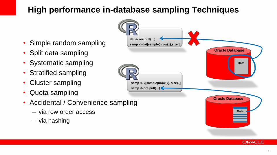
High performance in-database sampling Techniques

• Simple random sampling

• Split data sampling

• Systematic sampling

• Stratified sampling

• Cluster sampling

• Quota sampling

• Accidental / Convenience sampling

– via row order access

– via hashing

Data

Oracle Database

dat <- ore.pull(…)

samp <- dat[sample(nrow(x),size,]

Data

Oracle Database

samp <- x[sample(nrow(x), size),,]

samp <- ore.pull(…)

58

In-database Sampling Motivation

• R provides basic sampling capabilities, but requires data to be

pre-loaded into memory

• Catch 22

– Data too large to fit in memory, so need to sample

– Can’t sample because data won’t fit in memory

• Minimize data movement by sampling in Oracle Database

with ORE ordering framework’s integer row indexing

59

Simple random sampling Select rows at random

set.seed(1)

N <- 20

myData <- data.frame(a=1:N,b=letters[1:N])

MYDATA <- ore.push(myData)

head(MYDATA)

sampleSize <- 5

simpleRandomSample <- MYDATA[sample(nrow(MYDATA),

sampleSize), ,

drop=FALSE]

class(simpleRandomSample)

simpleRandomSample

60

Split data sampling Randomly partition data in train and test sets

set.seed(1)

sampleSize <- 5

ind <- sample(1:nrow(MYDATA),sampleSize)

group <- as.integer(1:nrow(MYDATA) %in% ind)

MYDATA.train <- MYDATA[group==FALSE,]

dim(MYDATA.train)

class(MYDATA.train)

MYDATA.test <- MYDATA[group==TRUE,]

dim(MYDATA.test)

61

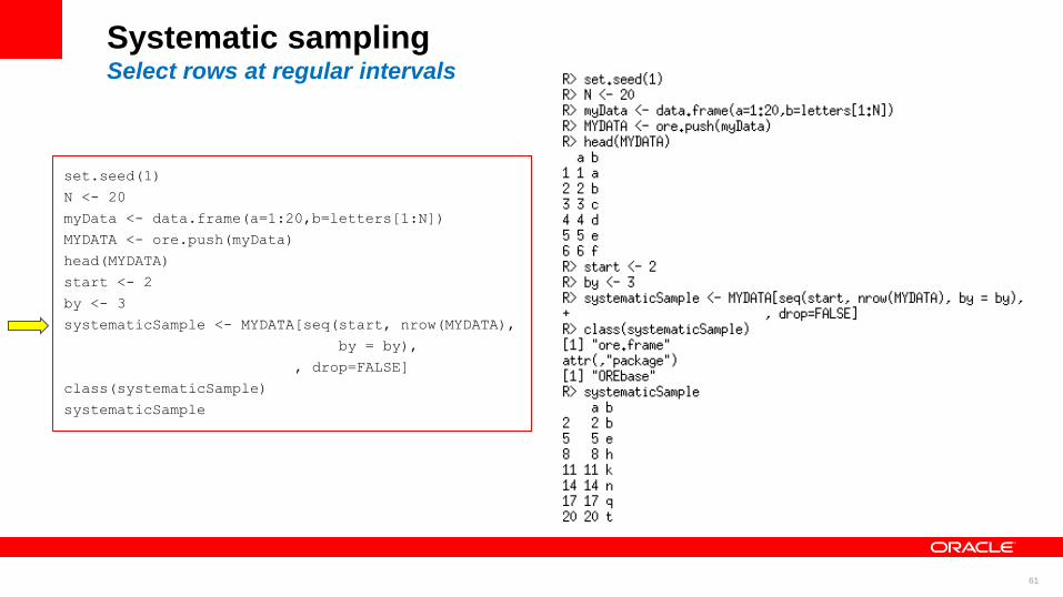
Systematic sampling Select rows at regular intervals

set.seed(1)

N <- 20

myData <- data.frame(a=1:20,b=letters[1:N])


head(MYDATA)

start <- 2

by <- 3

systematicSample <- MYDATA[seq(start, nrow(MYDATA),

by = by),

, drop=FALSE]

class(systematicSample)

systematicSample

62

Stratified sampling Select rows within each group

set.seed(1)

N <- 200

myData <- data.frame(a=1:N,b=round(rnorm(N),2),

group=round(rnorm(N,4),0))


head(MYDATA)

sampleSize <- 10

stratifiedSample <-

do.call(rbind,

lapply(split(MYDATA, MYDATA$group),

function(y) {

ny <- nrow(y)

y[sample(ny, sampleSize*ny/N),, drop = FALSE]

}))

class(stratifiedSample)

stratifiedSample

63

Cluster sampling Select whole groups at random

set.seed(1)

N <- 200

myData <- data.frame(a=1:N,b=round(runif(N),2),

group=round(rnorm(N,4),0))


head(MYDATA)

sampleSize <- 5

clusterSample <- do.call(rbind,

sample(split(MYDATA, MYDATA$group), 2))

class(clusterSample)

unique(clusterSample$group)

64

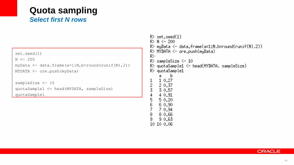
Quota sampling Select first N rows

set.seed(1)

N <- 200

myData <- data.frame(a=1:N,b=round(runif(N),2))


sampleSize <- 10

quotaSample1 <- head(MYDATA, sampleSize)

quotaSample1

65

High performance in-database sampling Techniques

• Simple random sampling

– x[sample(nrow(x), size), , drop=FALSE]

• Split data sampling

– nd <- sample(1:nrow(x),size); group <- as.integer(1:nrow(x) %in% ind)

– xTraining <- x[group==TRUE,]; xTest <- x[group==FALSE,]

• Systematic sampling

– x[seq(start, nrow(x), by = by), , drop=FALSE]

• Stratified sampling

– do.call(rbind, lapply(split(x, x$strata),

function(y) y[sample(nrow(y), size * nrow(y)/nrow(x)), , drop=FALSE]))

• Cluster sampling

– do.call(rbind, sample(split(x, x$cluster), size))

• Quota and Accidental sampling

– head(x, size) | tail(x, size) | x[indices, , drop = FALSE]

66

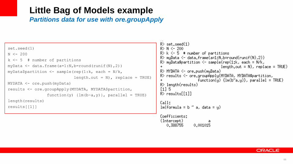
Little Bag of Models example Partitions data for use with ore.groupApply

set.seed(1)

N <- 200

k <- 5 # number of partitions

myData <- data.frame(a=1:N,b=round(runif(N),2))

myData$partition <- sample(rep(1:k, each = N/k,

length.out = N), replace = TRUE)


results <- ore.groupApply(MYDATA, MYDATA$partition,

function(y) {lm(b~a,y)}, parallel = TRUE)

length(results)

results[[1]]

67

ORE Column Name Length


68

Column Name Length

• Oracle Database tables and views limit

columns to 30 characters

• R data.frame column names can be

– arbitrarily long

– contain double quotes

– be non-unique

• ORE 1.3 supports R semantics for column

names of ore.frames

69

Long Column Names: Example

name1 <- 'a1234567890123456789012345678901234567890'

name2 <-

'b12345678901234567890123456789012345678901234567890'

df <- data.frame(x=1:3, y=1:3)

names(df) <- c(name1, name2)

df.ore <- ore.push(df)

df.ore

ore.create(df, table="DF")

Expected

70

Long Column Names: Example

ore.save(df.ore, name = "myDatastore")

ore.load("myDatastore")

df.ore

name3 <-

'c123456789012345678901234567890123456789012345__""'

names(df.ore) <- c(name3,name3)

df.ore

71

Data Types


72

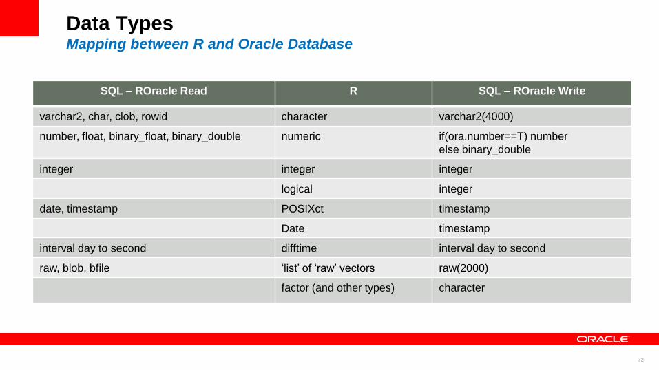
Data Types Mapping between R and Oracle Database

SQL – ROracle Read R SQL – ROracle Write

varchar2, char, clob, rowid character varchar2(4000)

number, float, binary_float, binary_double numeric if(ora.number==T) number

else binary_double

integer integer integer

logical integer

date, timestamp POSIXct timestamp

Date timestamp

interval day to second difftime interval day to second

raw, blob, bfile ‘list’ of ‘raw’ vectors raw(2000)

factor (and other types) character

73

Comparing R and ORE for building and scoring with linear models


74

Build a Regression Model Use distance and departure delay to predict arrival delay

Build in R

dat <- ore.pull(ONTIME_S)

mod <- lm(ARRDELAY ~ DISTANCE +

DEPDELAY, data=dat)

mod

summary(mod)

Build in ORE

dat <- ONTIME_S

mod.ore <- ore.lm(ARRDELAY ~ DISTANCE +

DEPDELAY, data=dat)

mod.ore

summary(mod.ore)


ORE is 42 X faster for user time

6 X faster for elapsed time

75

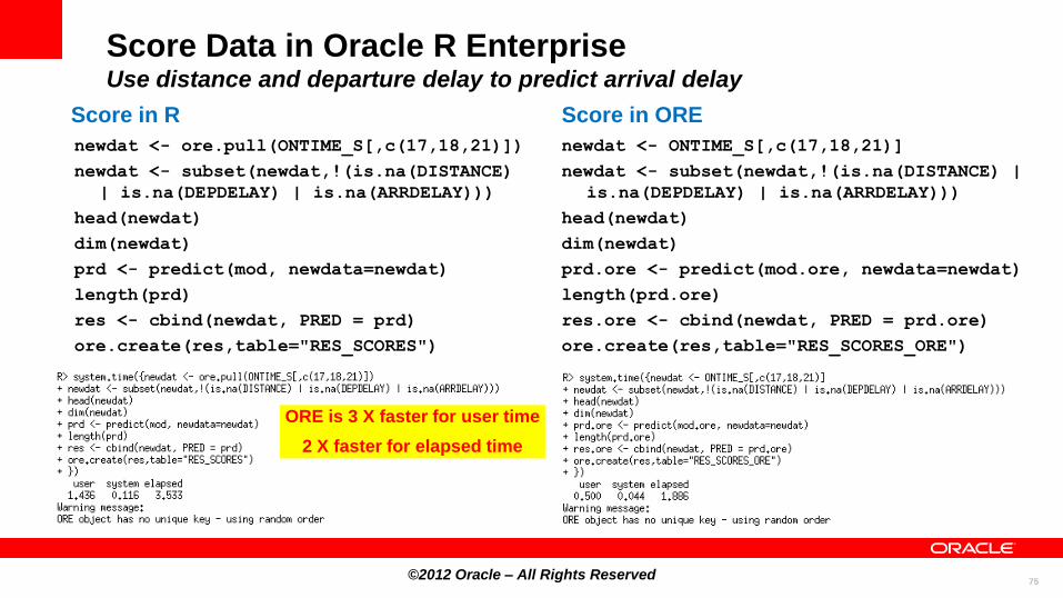
Score Data in Oracle R Enterprise Use distance and departure delay to predict arrival delay

Score in R

newdat <- ore.pull(ONTIME_S[,c(17,18,21)])

newdat <- subset(newdat,!(is.na(DISTANCE)

| is.na(DEPDELAY) | is.na(ARRDELAY)))

head(newdat)

dim(newdat)

prd <- predict(mod, newdata=newdat)

length(prd)

res <- cbind(newdat, PRED = prd)

ore.create(res,table="RES_SCORES")

Score in ORE

newdat <- ONTIME_S[,c(17,18,21)]

newdat <- subset(newdat,!(is.na(DISTANCE) |

is.na(DEPDELAY) | is.na(ARRDELAY)))

head(newdat)

dim(newdat)

prd.ore <- predict(mod.ore, newdata=newdat)

length(prd.ore)

res.ore <- cbind(newdat, PRED = prd.ore)

ore.create(res,table="RES_SCORES_ORE")


ORE is 3 X faster for user time

2 X faster for elapsed time

76

HIVE Transparency


77

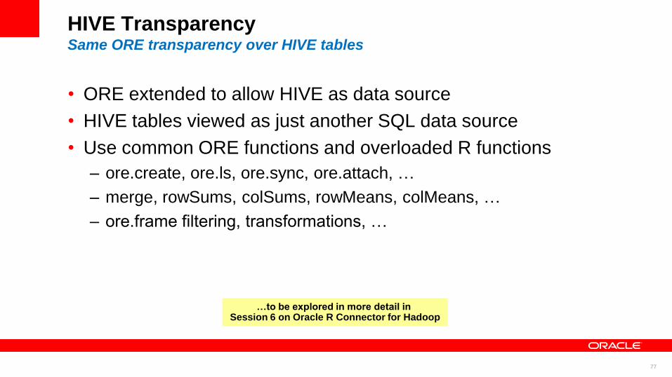
HIVE Transparency Same ORE transparency over HIVE tables

• ORE extended to allow HIVE as data source

• HIVE tables viewed as just another SQL data source

• Use common ORE functions and overloaded R functions

– ore.create, ore.ls, ore.sync, ore.attach, …

– merge, rowSums, colSums, rowMeans, colMeans, …

– ore.frame filtering, transformations, …

…to be explored in more detail in Session 6 on Oracle R Connector for Hadoop

78

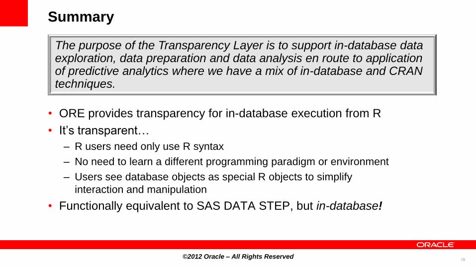
Summary

• ORE provides transparency for in-database execution from R

• It’s transparent…

– R users need only use R syntax

– No need to learn a different programming paradigm or environment

– Users see database objects as special R objects to simplify

interaction and manipulation

• Functionally equivalent to SAS DATA STEP, but in-database!


The purpose of the Transparency Layer is to support in-database data exploration, data preparation and data analysis en route to application of predictive analytics where we have a mix of in-database and CRAN techniques.

79

Resources

• Blog: https://blogs.oracle.com/R/

• Forum: https://forums.oracle.com/forums/forum.jspa?forumID=1397

• Oracle R Distribution:

http://www.oracle.com/technetwork/indexes/downloads/r-distribution-1532464.html

• ROracle:

http://cran.r-project.org/web/packages/ROracle

• Oracle R Enterprise:

http://www.oracle.com/technetwork/database/options/advanced-analytics/r-enterprise

• Oracle R Connector for Hadoop:

http://www.oracle.com/us/products/database/big-data-connectors/overview

https://blogs.oracle.com/R/

https://forums.oracle.com/forums/forum.jspa?forumID=1397



















oracle r enterprise 1.3 transparency layer

Documents