oracle database vldb and partitioning guide
TRANSCRIPT
8/16/2019 Oracle Database VLDB and Partitioning Guide
http://slidepdf.com/reader/full/oracle-database-vldb-and-partitioning-guide 1/304
Oracle® DatabaseVLDB and Partitioning Guide
11g Release 2 (11.2)
E16541-05
August 2010

8/16/2019 Oracle Database VLDB and Partitioning Guide
http://slidepdf.com/reader/full/oracle-database-vldb-and-partitioning-guide 2/304
Oracle Database VLDB and Partitioning Guide, 11 g Release 2 (11.2)
E16541-05
Copyright © 2008, 2010, Oracle and/or its affiliates. All rights reserved.
Contributors: Hermann Baer, Eric Belden, Jean-Pierre Dijcks, Steve Fogel, Lilian Hobbs, Paul Lane, Sue K.Lee, Diana Lorentz, Valarie Moore, Tony Morales, Mark Van de Wiel
This software and related documentation are provided under a license agreement containing restrictions on
use and disclosure and are protected by intellectual property laws. Except as expressly permitted in yourlicense agreement or allowed by law, you may not use, copy, reproduce, translate, broadcast, modify, license,transmit, distribute, exhibit, perform, publish, or display any part, in any form, or by any means. Reverseengineering, disassembly, or decompilation of this software, unless required by law for interoperability, isprohibited.
The information contained herein is subject to change without notice and is not warranted to be error-free. Ifyou find any errors, please report them to us in writing.
If this software or related documentation is delivered to the U.S. Government or anyone licensing it on behalf of the U.S. Government, the following notice is applicable:
U.S. GOVERNMENT RIGHTS Programs, software, databases, and related documentation and technical datadelivered to U.S. Government customers are "commercial computer software" or "commercial technical data"pursuant to the applicable Federal Acquisition Regulation and agency-specific supplemental regulations. Assuch, the use, duplication, disclosure, modification, and adaptation shall be subject to the restrictions andlicense terms set forth in the applicable Government contract, and, to the extent applicable by the terms ofthe Government contract, the additional rights set forth in FAR 52.227-19, Commercial Computer Software
License (December 2007). Oracle USA, Inc., 500 Oracle Parkway, Redwood City, CA 94065.
This software is developed for general use in a variety of information management applications. It is notdeveloped or intended for use in any inherently dangerous applications, including applications which maycreate a risk of personal injury. If you use this software in dangerous applications, then you shall beresponsible to take all appropriate fail-safe, backup, redundancy, and other measures to ensure the safe useof this software. Oracle Corporation and its affiliates disclaim any liability for any damages caused by use ofthis software in dangerous applications.
Oracle is a registered trademark of Oracle Corporation and/or its affiliates. Other names may be trademarksof their respective owners.
This software and documentation may provide access to or information on content, products, and servicesfrom third parties. Oracle Corporation and its affiliates are not responsible for and expressly disclaim allwarranties of any kind with respect to third-party content, products, and services. Oracle Corporation andits affiliates will not be responsible for any loss, costs, or damages incurred due to your access to or use ofthird-party content, products, or services.

8/16/2019 Oracle Database VLDB and Partitioning Guide
http://slidepdf.com/reader/full/oracle-database-vldb-and-partitioning-guide 3/304
iii
Contents
Preface ............................................................................................................................................................... xv
Audience..................................................................................................................................................... xv
Documentation Accessibility................................................................................................................... xv
Related Documents ............... .............. ................ .............. ............... .............. ............... .............. .............. xvi
Conventions .............. ............... .............. ............... .............. ................ .............. ................ ............... .......... xvi
What's New in Oracle Database to Support Very Large Databases? ........................ xvii
Oracle Database 11 g Release 2 (11.2.0.2) New Features to Support Very Large Databases.......... xvii
1 Introduction to Very Large Databases
Introduction to Partitioning ................................................................................................................... 1-1
VLDB and Partitioning ........................................................................................................................... 1-2
Partitioning As the Foundation for Information Lifecycle Management ..................................... 1-3
Partitioning for Every Database ............................................................................................................ 1-3
2 Partitioning ConceptsBasics of Partitioning............................................................................................................................... 2-1
Partitioning Key ................................................................................................................................. 2-2
Partitioned Tables .............................................................................................................................. 2-2
When to Partition a Table ............. .............. ................ .............. ............... ............... ................ ... 2-3
When to Partition an Index........................................................................................................ 2-3
Partitioned Index-Organized Tables ............... ............... .............. ................ .............. ............... ...... 2-3
System Partitioning............................................................................................................................ 2-3
Partitioning for Information Lifecycle Management ................ ............... ................ ............... ...... 2-3
Partitioning and LOB Data ............... .............. ................ .............. ............... ............... ................ ...... 2-4
Collections in XMLType and Object Data ............... ................ ............... ................ .............. .......... 2-4
Benefits of Partitioning ........................................................................................................................... 2-4Partitioning for Performance............................................................................................................ 2-5
Partition Pruning......................................................................................................................... 2-5
Partition-Wise Joins ................ .............. ............... .............. ................ ............. ................ ............ 2-5
Partitioning for Manageability......................................................................................................... 2-5
Partitioning for Availability ............................................................................................................. 2-6
Partitioning Strategies ............................................................................................................................. 2-6
Single-Level Partitioning................................................................................................................... 2-6
Range Partitioning ............. ............... .............. ................ .............. ............... ............... ............... . 2-7
8/16/2019 Oracle Database VLDB and Partitioning Guide
http://slidepdf.com/reader/full/oracle-database-vldb-and-partitioning-guide 4/304
iv
Hash Partitioning........................................................................................................................ 2-7
List Partitioning........................................................................................................................... 2-7
Composite Partitioning ............. ............... ............... ............... .............. ................ .............. ............... 2-8
Composite Range-Range Partitioning ............... ................ .............. ............... .............. ........... 2-8
Composite Range-Hash Partitioning .............. ................ .............. ............... .............. .............. 2-8
Composite Range-List Partitioning.......................................................................................... 2-9
Composite List-Range Partitioning.......................................................................................... 2-9Composite List-Hash Partitioning............................................................................................ 2-9
Composite List-List Partitioning............................................................................................... 2-9
Partitioning Extensions ........................................................................................................................... 2-9
Manageability Extensions................................................................................................................. 2-9
Interval Partitioning .............. .............. ................ .............. ............... ............... ............... ............ 2-9
Partition Advisor...................................................................................................................... 2-10
Partitioning Key Extensions .......................................................................................................... 2-10
Reference Partitioning............................................................................................................. 2-10
Virtual Column-Based Partitioning.......... ............... ............... ................ .............. ............... .. 2-11
Overview of Partitioned Indexes ....................................................................................................... 2-12
Local Partitioned Indexes............................................................................................................... 2-12Global Partitioned Indexes ............................................................................................................ 2-13
Global Range Partitioned Indexes ......................................................................................... 2-13
Global Hash Partitioned Indexes........................................................................................... 2-13
Maintenance of Global Partitioned Indexes......................................................................... 2-13
Global Nonpartitioned Indexes........... .............. ............... .............. ............... ............... .............. ... 2-14
Miscellaneous Information about Creating Indexes on Partitioned Tables .............. ............. 2-14
Partitioned Indexes on Composite Partitions ............................................................................. 2-15
3 Partitioning for Availability, Manageability, and Performance
Partition Pruning ...................................................................................................................................... 3-1Information That Can Be Used for Partition Pruning................................................................... 3-2
How to Identify Whether Partition Pruning has been Used ............. ................ .............. ............ 3-2
Static Partition Pruning .............. ............... ............... .............. ............... ............... .............. ............... 3-3
Dynamic Partition Pruning............................................................................................................... 3-3
Dynamic Pruning with Bind Variables.................................................................................... 3-4
Dynamic Pruning with Subqueries .............. ................ ............... ............... .............. ................ 3-4
Dynamic Pruning with Star Transformation ................. ............... .............. ............... ............. 3-5
Dynamic Pruning with Nested Loop Joins ............... .............. ............... ................ ............... .. 3-6
Partition Pruning Tips....................................................................................................................... 3-7
Data Type Conversions.............................................................................................................. 3-7
Function Calls.............................................................................................................................. 3-9Collection Tables...................................................................................................................... 3-10
Partition-Wise Joins .............................................................................................................................. 3-11
Full Partition-Wise Joins ................................................................................................................ 3-11
Full Partition-Wise Joins: Single-Level - Single-Level........................................................ 3-12
Full Partition-Wise Joins: Composite - Single-Level............... .............. ............... ............... 3-13
Full Partition-Wise Joins: Composite - Composite ............................................................. 3-15
Partial Partition-Wise Joins............................................................................................................ 3-16
Partial Partition-Wise Joins: Single-Level Partitioning.......... .............. ............... ............... . 3-16
8/16/2019 Oracle Database VLDB and Partitioning Guide
http://slidepdf.com/reader/full/oracle-database-vldb-and-partitioning-guide 5/304
v
Partial Partition-Wise Joins: Composite ............................................................................... 3-18
Index Partitioning ................................................................................................................................. 3-19
Local Partitioned Indexes............................................................................................................... 3-20
Local Prefixed Indexes ............................................................................................................ 3-21
Local Nonprefixed Indexes.......... .............. ............... .............. ................ ............... .............. ... 3-21
Global Partitioned Indexes ............................................................................................................ 3-22
Prefixed and Nonprefixed Global Partitioned Indexes.............. ............... ................ ......... 3-22Management of Global Partitioned Indexes ........................................................................ 3-22
Summary of Partitioned Index Types .......................................................................................... 3-23
The Importance of Nonprefixed Indexes..................................................................................... 3-24
Performance Implications of Prefixed and Nonprefixed Indexes........................ ................ .... 3-24
Guidelines for Partitioning Indexes ............................................................................................. 3-25
Physical Attributes of Index Partitions ........................................................................................ 3-25
Partitioning and Table Compression ................................................................................................. 3-26
Table Compression and Bitmap Indexes ..................................................................................... 3-27
Example of Table Compression and Partitioning ...................................................................... 3-27
Recommendations for Choosing a Partitioning Strategy .............................................................. 3-28
When to Use Range or Interval Partitioning............................................................................... 3-28When to Use Hash Partitioning .................................................................................................... 3-30
When to Use List Partitioning....................................................................................................... 3-31
When to Use Composite Partitioning............ ................ .............. ............... .............. ............... ..... 3-31
When to Use Composite Range-Hash Partitioning ............................................................ 3-32
When to Use Composite Range-List Partitioning ............................................................... 3-33
When to Use Composite Range-Range Partitioning................. ............... ............... ............ 3-33
When to Use Composite List-Hash Partitioning................................................................. 3-34
When to Use Composite List-List Partitioning.................................................................... 3-35
When to Use Composite List-Range Partitioning ............................................................... 3-35
When to Use Interval Partitioning................................................................................................ 3-36
When to Use Reference Partitioning ............................................................................................ 3-37
When to Partition on Virtual Columns........................................................................................ 3-38
Considerations When Using Read-Only Tablespaces ............................................................... 3-38
4 Partition Administration
Creating Partitions ................................................................................................................................... 4-1
Creating Range-Partitioned Tables and Global Indexes .............. ............... ............... ............... ... 4-2
Creating a Range-Partitioned Table ............. .............. ............... ............... .............. ............... ... 4-2
Creating a Range-Partitioned Global Index............................................................................ 4-3
Creating Interval-Partitioned Tables............................................................................................... 4-4
Creating Hash-Partitioned Tables and Global Indexes ............. .............. ............... ............... ....... 4-5Creating a Hash Partitioned Table ............... ................ .............. ............... ................ ............... 4-5
Creating a Hash-Partitioned Global Index.............................................................................. 4-6
Creating List-Partitioned Tables .............. ................. .............. ............... .............. .............. .............. 4-6
Creating Reference-Partitioned Tables ............... .............. ................ ............... .............. ................. 4-7
Creating Composite Partitioned Tables.......................................................................................... 4-9
Creating Composite Range-Hash Partitioned Tables............................................................ 4-9
Creating Composite Range-List Partitioned Tables......... .............. ................ .............. ....... 4-10
Creating Composite Range-Range Partitioned Tables....................................................... 4-12
8/16/2019 Oracle Database VLDB and Partitioning Guide
http://slidepdf.com/reader/full/oracle-database-vldb-and-partitioning-guide 6/304
vi
Creating Composite List-* Partitioned Tables ..................................................................... 4-14
Creating Composite Interval-* Partitioned Tables.............................................................. 4-16
Using Subpartition Templates to Describe Composite Partitioned Tables ............................ 4-19
Specifying a Subpartition Template for a *-Hash Partitioned Table ............... ............... .. 4-19
Specifying a Subpartition Template for a *-List Partitioned Table............. ................ ...... 4-20
Using Multicolumn Partitioning Keys......................................................................................... 4-21
Using Virtual Column-Based Partitioning .................................................................................. 4-23Using Table Compression with Partitioned Tables........... ............... .............. ............... ............. 4-24
Using Key Compression with Partitioned Indexes.................................................................... 4-25
Using Partitioning with Segments................................................................................................ 4-25
Deferred Segment Creation for Partitioning........................................................................ 4-25
Truncating Segments That Are Empty ................................................................................. 4-26
Maintenance Procedures for Segment Creation on Demand ............................................ 4-26
Creating Partitioned Index-Organized Tables .............. ............... .............. ................ .............. ... 4-26
Creating Range-Partitioned Index-Organized Tables ........................................................ 4-27
Creating Hash-Partitioned Index-Organized Tables ............. .............. ............... .............. .. 4-28
Creating List-Partitioned Index-Organized Tables................. ................ .............. .............. 4-28
Partitioning Restrictions for Multiple Block Sizes..................... ............... .............. ............... ..... 4-29Partitioning of Collections in XMLType and Objects ................................................................ 4-29
Performing PMOs on Partitions that Contain Collection Tables ............... ............... ........ 4-30
Maintaining Partitions ......................................................................................................................... 4-31
Updating Indexes Automatically................... ............... ............... ............... ............... .............. ..... 4-34
Adding Partitions............................................................................................................................ 4-35
Adding a Partition to a Range-Partitioned Table............. ............... ............... ............... ...... 4-35
Adding a Partition to a Hash-Partitioned Table.......... .............. ............... .............. ............. 4-36
Adding a Partition to a List-Partitioned Table .................................................................... 4-36
Adding a Partition to an Interval-Partitioned Table................. ............... .............. ............. 4-36
Adding Partitions to a Composite *-Hash Partitioned Table ............................................ 4-37
Adding Partitions to a Composite *-List Partitioned Table........................ ............... ........ 4-38
Adding Partitions to a Composite *-Range Partitioned Table .......................................... 4-39
Adding a Partition or Subpartition to a Reference-Partitioned Table................. ............. 4-39
Adding Index Partitions......... ............... ............... .............. ................ .............. ............... ........ 4-39
Coalescing Partitions ...................................................................................................................... 4-40
Coalescing a Partition in a Hash-Partitioned Table ............... ............... ................ .............. 4-41
Coalescing a Subpartition in a *-Hash Partitioned Table............ .............. ................ ......... 4-41
Coalescing Hash-partitioned Global Indexes ...................................................................... 4-41
Dropping Partitions ........................................................................................................................ 4-41
Dropping Table Partitions ...................................................................................................... 4-41
Dropping Interval Partitions.................................................................................................. 4-43
Dropping Index Partitions...................................................................................................... 4-44
Exchanging Partitions..................................................................................................................... 4-44
Exchanging a Range, Hash, or List Partition ....................................................................... 4-45
Exchanging a Partition of an Interval Partitioned Table...................... .............. ................ 4-45
Exchanging a Partition of a Reference Partitioned Table........... ............... .............. ........... 4-46
Exchanging a Partition of a Table with Virtual Columns.................................................. 4-46
Exchanging a Hash-Partitioned Table with a *-Hash Partition....................... ............... ... 4-46
Exchanging a Subpartition of a *-Hash Partitioned Table ............... ............... .............. ..... 4-47
8/16/2019 Oracle Database VLDB and Partitioning Guide
http://slidepdf.com/reader/full/oracle-database-vldb-and-partitioning-guide 7/304
vii
Exchanging a List-Partitioned Table with a *-List Partition .............. ............... ............... .. 4-47
Exchanging a Subpartition of a *-List Partitioned Table.................. ............... ............... .... 4-48
Exchanging a Range-Partitioned Table with a *-Range Partition .............. ............... ........ 4-48
Exchanging a Subpartition of a *-Range Partitioned Table ............................................... 4-49
Merging Partitions .......................................................................................................................... 4-49
Merging Range Partitions....................................................................................................... 4-50
Merging Interval Partitions .................................................................................................... 4-51Merging List Partitions ........................................................................................................... 4-52
Merging *-Hash Partitions...................................................................................................... 4-52
Merging *-List Partitions......................................................................................................... 4-52
Merging *-Range Partitions .................................................................................................... 4-54
Modifying Default Attributes...................... ................ ............... ............... ............... ............... ...... 4-54
Modifying Default Attributes of a Table.............................................................................. 4-54
Modifying Default Attributes of a Partition ........................................................................ 4-55
Modifying Default Attributes of Index Partitions.................... ............... ................ ............ 4-55
Modifying Real Attributes of Partitions ...................................................................................... 4-55
Modifying Real Attributes for a Range or List Partition.............. ............... .............. ......... 4-55
Modifying Real Attributes for a Hash Partition.................................................................. 4-56Modifying Real Attributes of a Subpartition....................................................................... 4-56
Modifying Real Attributes of Index Partitions .................................................................... 4-56
Modifying List Partitions: Adding Values .................................................................................. 4-56
Adding Values for a List Partition ............... .............. ............... ............... .............. .............. . 4-56
Adding Values for a List Subpartition.................................................................................. 4-57
Modifying List Partitions: Dropping Values...................... .............. ............... ............... ............. 4-57
Dropping Values from a List Partition ............... ................ ............... ............... ............... .... 4-57
Dropping Values from a List Subpartition .............. ............... ............... ............... ............... 4-58
Modifying a Subpartition Template ............................................................................................. 4-58
Moving Partitions............................................................................................................................ 4-59
Moving Table Partitions.......................................................................................................... 4-59
Moving Subpartitions.............................................................................................................. 4-60
Moving Index Partitions ......................................................................................................... 4-60
Redefining Partitions Online......................................................................................................... 4-60
Redefining Partitions with Collection Tables ...................................................................... 4-60
Rebuilding Index Partitions........................................................................................................... 4-62
Rebuilding Global Index Partitions....................................................................................... 4-62
Rebuilding Local Index Partitions......................................................................................... 4-63
Renaming Partitions ....................................................................................................................... 4-63
Renaming a Table Partition .................................................................................................... 4-63
Renaming a Table Subpartition ............................................................................................. 4-64
Renaming Index Partitions ..................................................................................................... 4-64
Splitting Partitions .......................................................................................................................... 4-64
Splitting a Partition of a Range-Partitioned Table .............................................................. 4-65
Splitting a Partition of a List-Partitioned Table................................................................... 4-65
Splitting a Partition of an Interval-Partitioned Table ......................................................... 4-66
Splitting a *-Hash Partition.................. ............... ................ .............. ............... ................ ....... 4-66
Splitting Partitions in a *-List Partitioned Table...................... ............... .............. ............... 4-67
Splitting a *-Range Partition................................................................................................... 4-69
8/16/2019 Oracle Database VLDB and Partitioning Guide
http://slidepdf.com/reader/full/oracle-database-vldb-and-partitioning-guide 8/304
viii
Splitting Index Partitions ........................................................................................................ 4-70
Optimizing SPLIT PARTITION and SPLIT SUBPARTITION Operations................... ... 4-70
Truncating Partitions...................................................................................................................... 4-71
Truncating a Table Partition................................................................................................... 4-71
Truncating a Subpartition....................................................................................................... 4-73
Dropping Partitioned Tables............................................................................................................... 4-73
Partitioned Tables and Indexes Example .......................................................................................... 4-74Viewing Information About Partitioned Tables and Indexes ...................................................... 4-75
5 Using Partitioning for Information Lifecycle Management
What Is ILM? ............................................................................................................................................. 5-1
Oracle Database for ILM .............. .............. ................ .............. ............... ............... ............... ............ 5-2
Oracle Database Manages All Types of Data.......................................................................... 5-2
Regulatory Requirements .............. ............... ............... ............... ............... ................ ............... ........ 5-2
Implementing ILM Using Oracle Database ........................................................................................ 5-3
Step 1: Define the Data Classes .............. .............. ................ .............. ............... ............... .............. .. 5-3
Partitioning .................................................................................................................................. 5-4
The Lifecycle of Data ............... .............. ............... .............. ................ .............. ............... ........... 5-5
Step 2: Create Storage Tiers for the Data Classes .............. .............. ............... ............... .............. .. 5-5
Assigning Classes to Storage Tiers........................................................................................... 5-6
The Costs Savings of using Tiered Storage ............... ............... ................ ............... ............... . 5-7
Step 3: Create Data Access and Migration Policies ............... ............... ............... ............... ........... 5-7
Controlling Access to Data .............. ............... ............... ............... ................ .............. ............... 5-7
Moving Data using Partitioning .............. ................. .............. ............... ............... .............. ...... 5-8
Step 4: Define and Enforce Compliance Policies ............... ............... ............... .............. ................ 5-8
Data Retention............................................................................................................................. 5-9
Immutability ............. ................ .............. ............... ............... ............... ............... .............. ........... 5-9
Privacy.......................................................................................................................................... 5-9Auditing ....................................................................................................................................... 5-9
Expiration..................................................................................................................................... 5-9
The Benefits of an Online Archive ....................................................................................................... 5-9
Oracle ILM Assistant ............................................................................................................................ 5-10
Lifecycle Setup................................................................................................................................. 5-11
Logical Storage Tiers ............................................................................................................... 5-12
Lifecycle Definitions ................................................................................................................ 5-13
Lifecycle Tables ........................................................................................................................ 5-14
Preferences................................................................................................................................ 5-20
Lifecycle Management......... ............... .............. ................ .............. ............... .............. ................ ... 5-21
Lifecycle Events Calendar........... .............. ................ .............. .............. ............... .............. ..... 5-21Lifecycle Events........................................................................................................................ 5-21
Event Scan History............ ............... .............. ............... .............. .............. ............... ................ 5-22
Compliance & Security................................................................................................................... 5-23
Current Status........................................................................................................................... 5-23
Digital Signatures and Immutability.............. .............. ............... .............. ............... ............. 5-23
Privacy & Security ................................................................................................................... 5-23
Auditing .................................................................................................................................... 5-24
Reports.............................................................................................................................................. 5-25
8/16/2019 Oracle Database VLDB and Partitioning Guide
http://slidepdf.com/reader/full/oracle-database-vldb-and-partitioning-guide 9/304
ix
Implementing an ILM System Manually ......................................................................................... 5-25
6 Using Partitioning in a Data Warehouse Environment
What Is a Data Warehouse? .................................................................................................................... 6-1
Scalability .................................................................................................................................................. 6-1
Bigger Databases .............. .............. ............... .............. ............... ............... .............. ................. .......... 6-2
Bigger Individual tables: More Rows in Tables............................................................................. 6-2
More Users Querying the System.................................................................................................... 6-2
More Complex Queries ..................................................................................................................... 6-2
Performance............................................................................................................................................... 6-2
Partition Pruning................................................................................................................................ 6-3
Basic Partition Pruning Techniques ............. ................ ............... .............. ................ ............... 6-3
Advanced Partition Pruning Techniques ............... ............... ............... ............... ................ .... 6-3
Partition-Wise Joins ........................................................................................................................... 6-5
Full Partition-Wise Joins .............. ............... .............. ................ ............... .............. ................. ... 6-5
Partial Partition-Wise Joins........................................................................................................ 6-7
Benefits of Partition-Wise Joins................................................................................................. 6-8
Performance Considerations for Parallel Partition-Wise Joins ............... ............... .............. 6-9
Indexes and Partitioned Indexes...................................................................................................... 6-9
Local Partitioned Indexes ....................................................................................................... 6-10
Nonpartitioned Indexes .......................................................................................................... 6-10
Global Partitioned Indexes ..................................................................................................... 6-11
Partitioning and Data Compression...................................................................................... 6-12
Materialized Views and Partitioning.................................................................................... 6-12
Manageability ........................................................................................................................................ 6-13
Partition Exchange Load................................................................................................................ 6-13
Partitioning and Indexes ................................................................................................................ 6-14
Partitioning and Materialized View Refresh Strategies ............................................................ 6-15Removing Data from Tables.......................................................................................................... 6-15
Partitioning and Data Compression............................................................................................. 6-16
Gathering Statistics on Large Partitioned Tables ....................................................................... 6-16
7 Using Partitioning in an Online Transaction Processing Environment
What is an OLTP System? ....................................................................................................................... 7-1
Performance............................................................................................................................................... 7-3
Deciding Whether to Partition Indexes........................................................................................... 7-3
Using Index-Organized Tables .............. ............... .............. ................ .............. ............... ......... 7-4
Manageability ........................................................................................................................................... 7-5
Impact of a Partition Maintenance Operation on a Partitioned Table with Local Indexes..... 7-5Impact of a Partition Maintenance Operation on Global Indexes .............. ............... ............... .. 7-6
Common Partition Maintenance Operations in OLTP Environments....................................... 7-6
Removing (Purging) Old Data ............... ............... ................ .............. ............... ................ ....... 7-6
Moving and/or Merging Older Partitions to a Low Cost Storage Tier Device................. 7-6
8 Using Parallel Execution
Introduction to Parallel Execution ........................................................................................................ 8-1

8/16/2019 Oracle Database VLDB and Partitioning Guide
http://slidepdf.com/reader/full/oracle-database-vldb-and-partitioning-guide 10/304
x
When to Implement Parallel Execution ............... ................ .............. ............... .............. .............. .. 8-2
When Not to Implement Parallel Execution .............. ............... ................ .............. ............... ........ 8-2
Fundamental Hardware Requirements .............. ............... .............. ............... ............... .............. ... 8-2
Operations That Can Be Parallelized ............. .............. ............... ............... .............. ............... ........ 8-3
How Parallel Execution Works .............................................................................................................. 8-4
Parallelizing SQL Statements .............. ............... .............. ............... ............... .............. ................. ... 8-4
Dividing Work Among Parallel Execution Servers ............. ............... ............... .............. ...... 8-5Parallelism Between Operations............................................................................................... 8-6
Producer/Consumer Operations.............................................................................................. 8-7
How Parallel Execution Servers Communicate............................................................................. 8-8
Degree of Parallelism......................................................................................................................... 8-9
Manually Specifying the Degree of Parallelism ............. ............... ............... ............... ........... 8-9
Automatic Parallel Degree Policy.......................................................................................... 8-10
Controlling Automatic Degree of Parallelism ..................................................................... 8-11
In-Memory Parallel Execution ............................................................................................... 8-11
Adaptive Parallelism............................................................................................................... 8-12
Controlling Automatic DOP, Parallel Statement Queuing, and In-Memory Parallel
Execution 8-12Parallel Statement Queuing ........................................................................................................... 8-13
Managing Parallel Statement Queuing with Resource Manager.......... .............. .............. 8-14
Grouping Parallel Statements with a BEGIN_SQL_BLOCK .. END_SQL_BLOCK Block....... 8-18
Managing Parallel Statement Queuing with Hints................. ............... ............... .............. 8-19
The Parallel Execution Server Pool............................................................................................... 8-20
Processing without Enough Parallel Execution Servers .................................................... 8-20
Granules of Parallelism .................................................................................................................. 8-20
Block Range Granules ............................................................................................................. 8-20
Partition Granules.................................................................................................................... 8-21
Balancing the Workload................................................................................................................. 8-22Parallel Execution Using Oracle RAC.......................................................................................... 8-23
Limiting the Number of Available Instances.................. .............. ................ .............. ......... 8-23
Types of Parallelism.............................................................................................................................. 8-23
About Parallel Queries ................................................................................................................... 8-23
Parallel Queries on Index-Organized Tables....................................................................... 8-24
Nonpartitioned Index-Organized Tables ............................................................................. 8-24
Partitioned Index-Organized Tables..................................................................................... 8-24
Parallel Queries on Object Types........................................................................................... 8-24
Rules for Parallelizing Queries .............................................................................................. 8-25
About Parallel DDL Statements.................................................................................................... 8-25
DDL Statements That Can Be Parallelized........................................................................... 8-25CREATE TABLE ... AS SELECT in Parallel.......................................................................... 8-26
Recoverability and Parallel DDL ........................................................................................... 8-27
Space Management for Parallel DDL.................................................................................... 8-27
Storage Space When Using Dictionary-Managed Tablespaces............. ............... ............. 8-27
Free Space and Parallel DDL.................................................................................................. 8-28
Rules for DDL Statements ...................................................................................................... 8-29
Rules for [CREATE | REBUILD] INDEX or [MOVE | SPLIT] PARTITION.................. 8-29
Rules for CREATE TABLE AS SELECT................................................................................ 8-30

8/16/2019 Oracle Database VLDB and Partitioning Guide
http://slidepdf.com/reader/full/oracle-database-vldb-and-partitioning-guide 11/304
xi
About Parallel DML Operations................................................................................................... 8-31
When to Use Parallel DML..................................................................................................... 8-31
Enabling Parallel DML............................................................................................................ 8-32
Rules for UPDATE, MERGE, and DELETE ......................................................................... 8-33
Rules for INSERT ... SELECT ................................................................................................. 8-34
Transaction Restrictions for Parallel DML........................................................................... 8-35
Rollback Segments ................................................................................................................... 8-35Recovery for Parallel DML..................................................................................................... 8-35
Space Considerations for Parallel DML........... ............... .............. ............... ................ ......... 8-36
Restrictions on Parallel DML ................................................................................................. 8-36
Data Integrity Restrictions...................................................................................................... 8-37
Trigger Restrictions.................................................................................................................. 8-38
Distributed Transaction Restrictions...................... .............. ............... .............. .............. ...... 8-38
Examples of Distributed Transaction Parallelization ......................................................... 8-38
About Parallel Execution of Functions............. ............... ............... .............. ............... .............. ... 8-38
Functions in Parallel Queries ................................................................................................. 8-39
Functions in Parallel DML and DDL Statements................................................................ 8-39
About Other Types of Parallelism ................................................................................................ 8-39Summary of Parallelization Rules ......................................................................................... 8-40
Initializing and Tuning Parameters for Parallel Execution........................................................... 8-41
Using Default Parameter Settings.................... ............... ............... ............... ............... ................. 8-41
Forcing Parallel Execution for a Session...................................................................................... 8-42
Tuning General Parameters for Parallel Execution......................................................................... 8-42
Parameters Establishing Resource Limits for Parallel Operations .......................................... 8-43
PARALLEL_FORCE_LOCAL ................................................................................................ 8-43
PARALLEL_MAX_SERVERS ................................................................................................ 8-43
PARALLEL_MIN_PERCENT ................................................................................................ 8-44
PARALLEL_MIN_SERVERS.................................................................................................. 8-44
PARALLEL_MIN_TIME_THRESHOLD.............................................................................. 8-44
PARALLEL_SERVERS_TARGET.......................................................................................... 8-45
SHARED_POOL_SIZE............................................................................................................ 8-45
Computing Additional Memory Requirements for Message Buffers............. ................ . 8-46
Adjusting Memory After Processing Begins........................................................................ 8-47
Parameters Affecting Resource Consumption................. .............. ................ .............. ............... 8-48
PGA_AGGREGATE_TARGET .............................................................................................. 8-49
PARALLEL_EXECUTION_MESSAGE_SIZE ...................................................................... 8-49
Parameters Affecting Resource Consumption for Parallel DML and Parallel DDL...... 8-49
Parameters Related to I/O............................................................................................................. 8-51
DB_CACHE_SIZE.................................................................................................................. .. 8-52
DB_BLOCK_SIZE..................................................................................................................... 8-52
DB_FILE_MULTIBLOCK_READ_COUNT ......................................................................... 8-52
DISK_ASYNCH_IO and TAPE_ASYNCH_IO.................................................................... 8-52
Monitoring Parallel Execution Performance.................................................................................... 8-53
Monitoring Parallel Execution Performance with Dynamic Performance Views .............. ... 8-53
V$PX_BUFFER_ADVICE........................................................................................................ 8-53
V$PX_SESSION........................................................................................................................ 8-53
V$PX_SESSTAT........................................................................................................................ 8-53

8/16/2019 Oracle Database VLDB and Partitioning Guide
http://slidepdf.com/reader/full/oracle-database-vldb-and-partitioning-guide 12/304
xii
V$PX_PROCESS....................................................................................................................... 8-53
V$PX_PROCESS_SYSSTAT.................................................................................................... 8-53
V$PQ_SESSTAT ....................................................................................................................... 8-54
V$PQ_TQSTAT ........................................................................................................................ 8-54
V$RSRC_CONS_GROUP_HISTORY.................................................................................... 8-55
V$RSRC_CONSUMER_GROUP ........................................................................................... 8-55
V$RSRC_PLAN........................................................................................................................ 8-55V$RSRC_PLAN_HISTORY .................................................................................................... 8-55
V$RSRC_SESSION_INFO....................................................................................................... 8-55
Monitoring Session Statistics......................................................................................................... 8-55
Monitoring System Statistics ......................................................................................................... 8-56
Monitoring Operating System Statistics ...................................................................................... 8-57
Miscellaneous Parallel Execution Tuning Tips ............................................................................... 8-57
Creating and Populating Tables in Parallel...................... ............... .............. ............... ............... 8-58
Using EXPLAIN PLAN to Show Parallel Operations Plans.............. ................ ............... ........ 8-59
Example: Using EXPLAIN PLAN to Show Parallel Operations....................... ................ 8-59
Additional Considerations for Parallel DML.............................................................................. 8-60
Parallel DML and Direct-Path Restrictions.......................................................................... 8-60Limitation on the Degree of Parallelism............................................................................... 8-60
Increasing INITRANS ............................................................................................................. 8-60
Limitation on Available Number of Transaction Free Lists for Segments.............. ........ 8-60
Using Multiple Archivers ....................................................................................................... 8-61
Database Writer Process (DBWn) Workload ....................................................................... 8-61
[NO]LOGGING Clause........................................................................................................... 8-61
Creating Indexes in Parallel........................................................................................................... 8-62
Parallel DML Tips ........................................................................................................................... 8-63
Parallel DML Tip 1: INSERT .................................................................................................. 8-63
Parallel DML Tip 2: Direct-Path INSERT............................................................................. 8-63
Parallel DML Tip 3: Parallelizing INSERT, MERGE, UPDATE, and DELETE............... 8-64
Incremental Data Loading in Parallel .......................................................................................... 8-65
Updating the Table in Parallel ............................................................................................... 8-65
Inserting the New Rows into the Table in Parallel ............................................................. 8-66
Merging in Parallel .................................................................................................................. 8-66
9 Backing Up and Recovering VLDBs
Data Warehousing .................................................................................................................................... 9-1
Data Warehouse Characteristics .............. .............. ............... .............. ................ .............. ............... 9-2
Oracle Backup and Recovery ................................................................................................................. 9-2
Physical Database Structures Used in Recovering Data............................................................... 9-3Datafiles........................................................................................................................................ 9-3
Redo Logs..................................................................................................................................... 9-3
Control Files................................................................................................................................. 9-3
Backup Type ....................................................................................................................................... 9-4
Backup Tools....................................................................................................................................... 9-4
Recovery Manager (RMAN)...................................................................................................... 9-5
Oracle Enterprise Manager........................................................................................................ 9-5
Oracle Data Pump....................................................................................................................... 9-5

8/16/2019 Oracle Database VLDB and Partitioning Guide
http://slidepdf.com/reader/full/oracle-database-vldb-and-partitioning-guide 13/304
xiii
User-Managed Backups ............. ................ .............. ............... ................ .............. ............... ...... 9-6
Data Warehouse Backup and Recovery................................................................................................ 9-6
Recovery Time Objective (RTO)....................................................................................................... 9-6
Recovery Point Objective (RPO) .............. ................ ............... ............... .............. ................ ............ 9-7
More Data Means a Longer Backup Window ............... ............... .............. .............. .............. 9-7
Divide and Conquer ............... .............. ............... ............... ............... .............. ............... ............ 9-7
The Data Warehouse Recovery Methodology .................................................................................... 9-8Best Practice 1: Use ARCHIVELOG Mode.......................................................................................... 9-8
Is Downtime Acceptable? ................................................................................................................. 9-8
Best Practice 2: Use RMAN..................................................................................................................... 9-9
Best Practice 3: Use Block Change Tracking........................................................................................ 9-9
Best Practice 4: Use RMAN Multi-Section Backups.......................................................................... 9-9
Best Practice 5: Leverage Read-Only Tablespaces.............................................................................. 9-9
Best Practice 6: Plan for NOLOGGING Operations in Your Backup/Recovery Strategy ....... 9-10
Extract, Transform, and Load...................... .............. ................ .............. ............... .............. ......... 9-11
The Extract, Transform, and Load Strategy ................................................................................ 9-11
Incremental Backup........................................................................................................................ 9-12
The Incremental Approach ............................................................................................................ 9-12Flashback Database and Guaranteed Restore Points................. ................ ............... .............. ... 9-13
Best Practice 7: Not All Tablespaces Are Created Equal ................................................................ 9-13
10 Storage Management for VLDBs
High Availability ................................................................................................................................... 10-1
Hardware-Based Mirroring ........................................................................................................... 10-2
RAID 1 Mirroring..................................................................................................................... 10-2
RAID 5 Mirroring..................................................................................................................... 10-2
Mirroring using Oracle ASM......................................................................................................... 10-2
Performance............................................................................................................................................ 10-3Hardware-Based Striping .............................................................................................................. 10-3
RAID 0 Striping ........................................................................................................................ 10-4
RAID 5 Striping ........................................................................................................................ 10-4
Striping Using Oracle ASM ........................................................................................................... 10-4
Information Lifecycle Management ............................................................................................. 10-4
Partition Placement......................................................................................................................... 10-5
Bigfile Tablespaces.......................................................................................................................... 10-5
Oracle Database File System (DBFS) ............................................................................................ 10-5
Scalability and Manageability............................................................................................................ 10-6
Stripe and Mirror Everything (SAME)......... ............... .............. ............... ............... .............. ....... 10-6
SAME and Manageability.............................................................................................................. 10-6Oracle ASM Settings Specific to VLDBs .......................................................................................... 10-6
Monitoring Database Storage Using Database Control ................................................................ 10-7
Index

8/16/2019 Oracle Database VLDB and Partitioning Guide
http://slidepdf.com/reader/full/oracle-database-vldb-and-partitioning-guide 14/304
xiv
8/16/2019 Oracle Database VLDB and Partitioning Guide
http://slidepdf.com/reader/full/oracle-database-vldb-and-partitioning-guide 15/304
xv
Preface
This book contains an overview of very large database (VLDB) topics, with emphasison partitioning as a key component of the VLDB strategy. Partitioning enhances theperformance, manageability, and availability of a wide variety of applications andhelps reduce the total cost of ownership for storing large amounts of data.
AudienceThis document is intended for database administrators (DBAs) and developers whocreate, manage, and write applications for very large databases (VLDB).
Documentation AccessibilityOur goal is to make Oracle products, services, and supporting documentationaccessible to all users, including users that are disabled. To that end, ourdocumentation includes features that make information available to users of assistivetechnology. This documentation is available in HTML format, and contains markup tofacilitate access by the disabled community. Accessibility standards will continue toevolve over time, and Oracle is actively engaged with other market-leading
technology vendors to address technical obstacles so that our documentation can beaccessible to all of our customers. For more information, visit the Oracle AccessibilityProgram Web site at http://www.oracle.com/accessibility/ .
Accessibility of Code Examples in Documentation
Screen readers may not always correctly read the code examples in this document. Theconventions for writing code require that closing braces should appear on anotherwise empty line; however, some screen readers may not always read a line of textthat consists solely of a bracket or brace.
Accessibility of Links to External Web Sites in Documentation
This documentation may contain links to Web sites of other companies or
organizations that Oracle does not own or control. Oracle neither evaluates nor makesany representations regarding the accessibility of these Web sites.
Access to Oracle Support
Oracle customers have access to electronic support through My Oracle Support. Forinformation, visit http://www.oracle.com/support/contact.html or visithttp://www.oracle.com/accessibility/support.html if you are hearingimpaired.

8/16/2019 Oracle Database VLDB and Partitioning Guide
http://slidepdf.com/reader/full/oracle-database-vldb-and-partitioning-guide 16/304
xvi
Related DocumentsFor more information, see the following documents in the Oracle Databasedocumentation set:
■ Oracle Database Concepts
■ Oracle Database Administrator's Guide
■ Oracle Database SQL Language Reference
■ Oracle Database Data Warehousing Guide
■ Oracle Database Performance Tuning Guide
ConventionsThe following text conventions are used in this document:
Convention Meaning
boldface Boldface type indicates graphical user interface elements associated
with an action, or terms defined in text or the glossary.italic Italic type indicates book titles, emphasis, or placeholder variables for
which you supply particular values.
monospace Monospace type indicates commands within a paragraph, URLs, codein examples, text that appears on the screen, or text that you enter.
8/16/2019 Oracle Database VLDB and Partitioning Guide
http://slidepdf.com/reader/full/oracle-database-vldb-and-partitioning-guide 17/304
xvii
What's New in Oracle Database to SupportVery Large Databases?
This chapter describes new features in Oracle Database to support very largedatabases (VLDB).
Oracle Database 11g Release 2 (11.2.0.2) New Features to Support VeryLarge Databases
These are the new features in Oracle Database 11 g Release 2 (11.2.0.2) to support verylarge databases:
■ Enhancements for managing segments
– Segment creation on demand for partitioned tables
This feature enables the creation of partitioned tables with deferred segmentcreation. With this feature, on-disk segments are not created for a subpartitionand its dependent objects until the first row is inserted.
For information about partitioning, refer to "Using Partitioning withSegments" on page 4-25.
– Enhanced TRUNCATE functionality
If a partition or subpartition has a segment, the truncate feature drops thesegment if the DROP ALL STORAGE clause is specified.
For information about partitioning, refer to "Using Partitioning withSegments" on page 4-25.
– Maintenance package for segment creation on demand
New procedures are added to the PL/SQL DBMS_SPACE_ADMIN package toenable you to maintain segment creation on demand.
For information about partitioning, refer to "Using Partitioning withSegments" on page 4-25.
■ Managing Parallel Statement Queuing
By default, parallel statements are dequeued from the parallel statement queue ina simple first in, first out (FIFO) order. This feature enables you to use resource
Note: This functionality is available starting with Oracle Database11g Release 2 (11.2.0.2).
8/16/2019 Oracle Database VLDB and Partitioning Guide
http://slidepdf.com/reader/full/oracle-database-vldb-and-partitioning-guide 18/304
xviii
manager to manage the parallel statement queue by configuring a resource planthat controls the order in which parallel statements are dequeued. For example,you can ensure that parallel statements associated with a high-priority workloador consumer group are dequeued ahead of parallel statements from low-priorityconsumer groups. Alternatively, you could implement a fair-share policy thatdequeues parallel statements based on the resource allocations configured for eachconsumer group.
For information about parallel statement queuing, refer to "Parallel StatementQueuing" on page 8-13. For information about managing parallel statementqueuing, refer to "Managing Parallel Statement Queuing with Resource Manager" on page 8-14.
See Also:
■ Oracle Database Concepts for information about parallel queryprocessing
■ Oracle Database SQL Language Reference for information about thePARALLEL hint
■ Oracle Database PL/SQL Packages and Types Reference for
information about the DBMS_RESOURCE_MANAGER package
8/16/2019 Oracle Database VLDB and Partitioning Guide
http://slidepdf.com/reader/full/oracle-database-vldb-and-partitioning-guide 19/304
1
Introduction to Very Large Databases 1-1
1Introduction to Very Large Databases
Modern enterprises frequently run mission-critical databases containing upwards ofseveral hundred gigabytes, and often several terabytes of data. These enterprises arechallenged by the support and maintenance requirements of very large databases(VLDB), and must devise methods to meet those challenges.
This chapter contains an overview of VLDB topics, with emphasis on partitioning as akey component of the VLDB strategy.
■ Introduction to Partitioning
■ VLDB and Partitioning
■ Partitioning As the Foundation for Information Lifecycle Management
■ Partitioning for Every Database
Introduction to PartitioningPartitioning addresses key issues in supporting very large tables and indexes bydecomposing them into smaller and more manageable pieces called partitions, whichare entirely transparent to an application. SQL queries and DML statements do notneed to be modified to access partitioned tables. However, after partitions are defined,DDL statements can access and manipulate individual partitions rather than entiretables or indexes. This is how partitioning can simplify the manageability of largedatabase objects.
Each partition of a table or index must have the same logical attributes, such ascolumn names, data types, and constraints, but each partition can have separatephysical attributes such as compression enabled or disabled, physical storage settings,and tablespaces.
Partitioning is useful for many different types of applications, particularly applicationsthat manage large volumes of data. OLTP systems often benefit from improvements inmanageability and availability, while data warehousing systems benefit fromperformance and manageability.
Partitioning offers these advantages:
■ It enables data management operations such as data loads, index creation andrebuilding, and backup/recovery at the partition level, rather than on the entiretable. This results in significantly reduced times for these operations.
Note: Partitioning functionality is available only if you purchase thePartitioning option.
8/16/2019 Oracle Database VLDB and Partitioning Guide
http://slidepdf.com/reader/full/oracle-database-vldb-and-partitioning-guide 20/304
VLDB and Partitioning
1-2 Oracle Database VLDB and Partitioning Guide
■ It improves query performance. Often the results of a query can be achieved byaccessing a subset of partitions, rather than the entire table. For some queries, thistechnique (called partition pruning) can provide order-of-magnitude gains inperformance.
■ It significantly reduces the impact of scheduled downtime for maintenanceoperations.
Partition independence for partition maintenance operations lets you performconcurrent maintenance operations on different partitions of the same table orindex. You can also run concurrent SELECT and DML operations against partitionsthat are unaffected by maintenance operations.
■ It increases the availability of mission-critical databases if critical tables andindexes are divided into partitions to reduce the maintenance windows, recoverytimes, and impact of failures.
■ Parallel execution provides specific advantages to optimize resource utilization,and minimize execution time. Parallel execution against partitioned objects is keyfor scalability in a clustered environment. Parallel execution is supported forqueries and for DML and DDL.
Partitioning enables faster data access within an Oracle database. Whether a databasehas 10 GB or 10 TB of data, partitioning can improve data access by orders ofmagnitude. Partitioning can be implemented without requiring any modifications toyour applications. For example, you could convert a nonpartitioned table to apartitioned table without needing to modify any of the SELECT statements or DMLstatements which access that table. You do not need to rewrite your application code totake advantage of partitioning.
VLDB and PartitioningA very large database has no minimum absolute size. Although a VLDB is a databaselike smaller databases, there are specific challenges in managing a VLDB. Thesechallenges are related to the sheer size, and the cost-effectiveness of performingoperations against a system that size, taken for granted on smaller databases.
Several trends have been responsible for the steady growth in database size:
■ For a long time, systems have been developed in isolation. Companies havestarted to see the benefits of combining these systems to enable cross-departmentalanalysis while reducing system maintenance costs. Consolidation of databases andapplications is a key factor in the ongoing growth of database size.
■ Many companies face regulations that set specific requirements for storing data fora minimum amount of time. The regulations generally result in more data beingstored for longer periods of time.
■ Companies grow by expanding sales and operations or through mergers and
acquisitions, causing the amount of generated and processed data to increase. Atthe same time, the user population that relies on the database for daily activitiesincreases.
Partitioning is a critical feature for managing very large databases. Growth is the basicchallenge that partitioning addresses for very large databases, and partitioning enablesa divide and conquer technique for managing the tables and indexes in the database,especially as those tables and indexes grow. Partitioning is the feature that allows adatabase to scale for very large data sets while maintaining consistent performance,without unduly increasing administrative or hardware resources. Chapter 3,
8/16/2019 Oracle Database VLDB and Partitioning Guide
http://slidepdf.com/reader/full/oracle-database-vldb-and-partitioning-guide 21/304
Partitioning for Every Database
Introduction to Very Large Databases 1-3
"Partitioning for Availability, Manageability, and Performance" provides availability,manageability, and performance considerations for partitioning implementations.
Chapter 9, "Backing Up and Recovering VLDBs" addresses the challenges surrounding backup and recovery for a VLDB.
Storage is a key component of a very large database. Chapter 10, "StorageManagement for VLDBs" focuses on best practices for storage in a VLDB.
Partitioning As the Foundation for Information Lifecycle ManagementInformation Lifecycle Management (ILM) is a set of processes and policies formanaging data throughout its useful life. One important component of an ILMstrategy is determining the most appropriate and cost-effective medium for storingdata at any point during its life time: newer data used in day-to-day operations isstored on the fastest, most highly-available storage tier, while older data which isaccessed infrequently may be stored on a less expensive and less performant storagetier. Older data may also be updated less frequently in which case it makes sense tocompress and store the data as read-only.
Oracle Database provides the ideal environment for implementing your ILM solution.
Oracle supports multiple storage tiers, and because all of the data remains in theOracle database, the use of multiple storage tiers is completely transparent to theapplication and the data continues to be completely secure. Partitioning provides thefundamental technology that enables data in tables to be stored in different partitions.
Although multiple storage tiers and sophisticated ILM policies are most often found inenterprise-level systems, most companies and most databases need some degree ofinformation lifecycle management. The most basic of ILM operations, archiving olderdata and purging or removing that data from the database, can be orders of magnitudefaster when using partitioning.
For more information about ILM, see Chapter 5, "Using Partitioning for InformationLifecycle Management".
Partitioning for Every DatabaseThe benefits of partitioning are not just for very large databases; every database, evensmall databases, can benefit from partitioning. While partitioning is a necessity for thelargest databases in the world, partitioning is obviously beneficial for the smallerdatabase as well. Even a database whose size is measured in megabytes can gain thesame type of performance and manageability benefits from partitioning as the largestmulti-terabyte systems.
For more information about how partitioning can provide benefits in a datawarehouse environment, see Chapter 6, "Using Partitioning in a Data WarehouseEnvironment".
For more information about how partitioning can provide benefits in an OLTPenvironment, see Chapter 7, "Using Partitioning in an Online Transaction ProcessingEnvironment".
8/16/2019 Oracle Database VLDB and Partitioning Guide
http://slidepdf.com/reader/full/oracle-database-vldb-and-partitioning-guide 22/304
Partitioning for Every Database
1-4 Oracle Database VLDB and Partitioning Guide
8/16/2019 Oracle Database VLDB and Partitioning Guide
http://slidepdf.com/reader/full/oracle-database-vldb-and-partitioning-guide 23/304
2
Partitioning Concepts 2-1
2Partitioning Concepts
Partitioning enhances the performance, manageability, and availability of a widevariety of applications and helps reduce the total cost of ownership for storing largeamounts of data. Partitioning allows tables, indexes, and index-organized tables to besubdivided into smaller pieces, enabling these database objects to be managed andaccessed at a finer level of granularity. Oracle provides a rich variety of partitioningstrategies and extensions to address every business requirement. Because it is entirely
transparent, partitioning can be applied to almost any application without the need forpotentially expensive and time consuming application changes.
This chapter contains the following topics:
■ Basics of Partitioning
■ Benefits of Partitioning
■ Partitioning Strategies
■ Partitioning Extensions
■ Overview of Partitioned Indexes
Basics of PartitioningPartitioning allows a table, index, or index-organized table to be subdivided intosmaller pieces, where each piece of such a database object is called a partition. Eachpartition has its own name, and may optionally have its own storage characteristics.
From the perspective of a database administrator, a partitioned object has multiplepieces that can be managed either collectively or individually. This gives theadministrator considerable flexibility in managing partitioned objects. However, fromthe perspective of the application, a partitioned table is identical to a nonpartitionedtable; no modifications are necessary when accessing a partitioned table using SQLqueries and DML statements.
Figure 2–1 offers a graphical view of how partitioned tables differ from nonpartitioned
tables.
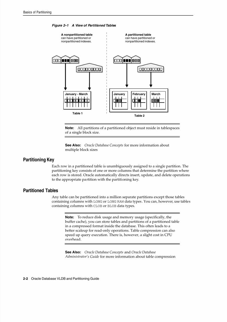
8/16/2019 Oracle Database VLDB and Partitioning Guide
http://slidepdf.com/reader/full/oracle-database-vldb-and-partitioning-guide 24/304
Basics of Partitioning
2-2 Oracle Database VLDB and Partitioning Guide
Figure 2–1 A View of Partitioned Tables
Partitioning KeyEach row in a partitioned table is unambiguously assigned to a single partition. Thepartitioning key consists of one or more columns that determine the partition whereeach row is stored. Oracle automatically directs insert, update, and delete operationsto the appropriate partition with the partitioning key.
Partitioned TablesAny table can be partitioned into a million separate partitions except those tablescontaining columns with LONG or LONG RAW data types. You can, however, use tablescontaining columns with CLOB or BLOB data types.
Note: All partitions of a partitioned object must reside in tablespacesof a single block size.
See Also: Oracle Database Concepts for more information aboutmultiple block sizes
Note: To reduce disk usage and memory usage (specifically, the buffer cache), you can store tables and partitions of a partitioned table
in a compressed format inside the database. This often leads to a better scaleup for read-only operations. Table compression can alsospeed up query execution. There is, however, a slight cost in CPUoverhead.
See Also: Oracle Database Concepts and Oracle Database Administrator's Guide for more information about table compression
A nonpartitioned tablecan have partitioned ornonpartitioned indexes.
A partitioned tablecan have partitioned ornonpartitioned indexes.
Table 1
January - March January
Table 2
February March
8/16/2019 Oracle Database VLDB and Partitioning Guide
http://slidepdf.com/reader/full/oracle-database-vldb-and-partitioning-guide 25/304
Basics of Partitioning
Partitioning Concepts 2-3
When to Partition a Table
Here are some suggestions for when to partition a table:
■ Tables greater than 2 GB should always be considered as candidates forpartitioning.
■ Tables containing historical data, in which new data is added into the newestpartition. A typical example is a historical table where only the current month'sdata is updatable and the other 11 months are read only.
■ When the contents of a table must be distributed across different types of storagedevices.
When to Partition an Index
Here are some suggestions for when to consider partitioning an index:
■ Avoid rebuilding the entire index when data is removed.
■ Perform maintenance on parts of the data without invalidating the entire index.
■ Reduce the impact of index skew caused by an index on a column with amonotonically increasing value.
Partitioned Index-Organized TablesPartitioned index-organized tables are very useful for providing improvedperformance, manageability, and availability for index-organized tables.
For partitioning an index-organized table:
■ Partition columns must be a subset of the primary key columns.
■ Secondary indexes can be partitioned (both locally and globally).
■ OVERFLOW data segments are always equipartitioned with the table partitions.
System PartitioningSystem partitioning enables application-controlled partitioning without having thedatabase controlling the data placement. The database simply provides the ability to break down a table into partitions without knowing what the individual partitions aregoing to be used for. All aspects of partitioning have to be controlled by theapplication. For example, an attempt to insert into a system partitioned table withoutthe explicit specification of a partition fail.
System partitioning provides the well-known benefits of partitioning (scalability,availability, and manageability), but the partitioning and actual data placement are
controlled by the application.
Partitioning for Information Lifecycle ManagementInformation Lifecycle Management (ILM) is concerned with managing data during itslifetime. Partitioning plays a key role in ILM because it enables groups of data (that is,partitions) to be distributed across different types of storage devices and managedindividually.
See Also: Oracle Database Concepts for more information about
index-organized tables
See Also: Oracle Database Data Cartridge Developer's Guide for moreinformation about system partitioning

8/16/2019 Oracle Database VLDB and Partitioning Guide
http://slidepdf.com/reader/full/oracle-database-vldb-and-partitioning-guide 26/304
Benefits of Partitioning
2-4 Oracle Database VLDB and Partitioning Guide
For more information about Information Lifecycle Management, see Chapter 5, "UsingPartitioning for Information Lifecycle Management".
Partitioning and LOB DataUnstructured data (such as images and documents) which is stored in a LOB columnin the database can also be partitioned. When a table is partitioned, all the columns
reside in the tablespace for that partition, except LOB columns, which can be stored intheir own tablespace.
This technique is very useful when a table consists of large LOBs because they can bestored separately from the main data. This can be beneficial if the main data is beingfrequently updated but the LOB data is not. For example, an employee record maycontain a photo which is unlikely to change frequently. However, the employeepersonnel details (such as address, department, manager, and so on) could change.This approach also means that cheaper storage can be used for storing the LOB dataand more expensive, faster storage used for the employee record.
Collections in XMLType and Object Data
Partitioning when using XMLType and object tables and columns offers the standardadvantages of partitioning, such as allowing tables, and indexes to be subdivided intosmaller pieces, thus enabling these database objects to be managed and accessed at afiner level of granularity.
When you partition an XMLType table or a table with an XMLType column using list,range, or hash partitioning, any ordered collection tables (OCTs) within the data areautomatically partitioned accordingly, by default. This equipartitioning means that thepartitioning of an OCT follows the partitioning scheme of its parent (base) table. Thereis a corresponding collection-table partition for each partition of the base table. A childelement is stored in the collection-table partition that corresponds to the base-tablepartition of its parent element.
If you partition a table that has a nested table, Oracle Database uses the partitioning
scheme of the original base table as the basis for how the nested table is partitioned.This partitioning of one base table partition for each nested table partition is calledequipartitioning. By default, nested tables are automatically partitioned when the basetable is partitioned. Note, however, that composite partitioning is not supported forOCTs or nested tables.
For information about partitioning an XMLType table, refer to "Partitioning ofCollections in XMLType and Objects" on page 4-29.
Benefits of PartitioningPartitioning can provide tremendous benefit to a wide variety of applications byimproving performance, manageability, and availability. It is not unusual forpartitioning to improve the performance of certain queries or maintenance operations by an order of magnitude. Moreover, partitioning can greatly simplify commonadministration tasks.
Partitioning also enables database designers and administrators to tackle somedifficult problems posed by cutting-edge applications. Partitioning is a key tool for
See Also:
■ Oracle Database Object-Relational Developer's Guide
■ Oracle Database SQL Language Reference for syntax of nested tables
8/16/2019 Oracle Database VLDB and Partitioning Guide
http://slidepdf.com/reader/full/oracle-database-vldb-and-partitioning-guide 27/304
Benefits of Partitioning
Partitioning Concepts 2-5
building multi-terabyte systems or systems with extremely high availabilityrequirements.
Partitioning for PerformanceBy limiting the amount of data to be examined or operated on, and by providing datadistribution for parallel execution, partitioning provides multiple performance
benefits. These features include:
■ Partition Pruning
■ Partition-Wise Joins
Partition Pruning
Partition pruning is the simplest and also the most substantial means to improveperformance using partitioning. Partition pruning can often improve queryperformance by several orders of magnitude. For example, suppose an applicationcontains an Orders table containing a historical record of orders, and that this tablehas been partitioned by week. A query requesting orders for a single week would onlyaccess a single partition of the Orders table. If the Orders table had 2 years of
historical data, then this query would access one partition instead of 104 partitions.This query could potentially execute 100 times faster simply because of partitionpruning.
Partition pruning works with all of Oracle's other performance features. Oracle usespartition pruning with any indexing technique, join technique, or parallel accessmethod.
Partition-Wise Joins
Partitioning can also improve the performance of multi-table joins by using atechnique known as partition-wise joins. Partition-wise joins can be applied when twotables are being joined and both tables are partitioned on the join key, or when areference partitioned table is joined with its parent table. Partition-wise joins break a
large join into smaller joins that occur between each of the partitions, completing theoverall join in less time. This offers significant performance benefits both for serial andparallel execution.
Partitioning for ManageabilityPartitioning allows tables and indexes to be partitioned into smaller, more manageableunits, providing database administrators with the ability to pursue a divide and conquer approach to data management. With partitioning, maintenance operations can befocused on particular portions of tables. For example, a database administrator could back up a single partition of a table, rather than backing up the entire table. Formaintenance operations across an entire database object, it is possible to perform theseoperations on a per-partition basis, thus dividing the maintenance process into moremanageable chunks.
A typical usage of partitioning for manageability is to support a rolling window loadprocess in a data warehouse. Suppose that a DBA loads new data into a table on aweekly basis. That table could be partitioned so that each partition contains one weekof data. The load process is simply the addition of a new partition using a partitionexchange load. Adding a single partition is much more efficient than modifying theentire table, because the DBA does not need to modify any other partitions.

8/16/2019 Oracle Database VLDB and Partitioning Guide
http://slidepdf.com/reader/full/oracle-database-vldb-and-partitioning-guide 28/304
Partitioning Strategies
2-6 Oracle Database VLDB and Partitioning Guide
Partitioning for AvailabilityPartitioned database objects provide partition independence. This characteristic ofpartition independence can be an important part of a high-availability strategy. Forexample, if one partition of a partitioned table is unavailable, then all of the otherpartitions of the table remain online and available. The application can continue toexecute queries and transactions against the available partitions for the table, and
these database operations run successfully, provided they do not need to access theunavailable partition.
The database administrator can specify that each partition be stored in a separatetablespace; the most common scenario is having these tablespaces stored on differentstorage tiers. Storing different partitions in different tablespaces allows the databaseadministrator to do backup and recovery operations on each individual partition,independent of the other partitions in the table. Thus allowing the active parts of thedatabase to be made available sooner so access to the system can continue, while theinactive data is still being restored. Moreover, partitioning can reduce scheduleddowntime. The performance gains provided by partitioning may enable databaseadministrators to complete maintenance operations on large database objects inrelatively small batch windows.
Partitioning StrategiesOracle Partitioning offers three fundamental data distribution methods as basicpartitioning strategies that control how data is placed into individual partitions:
■ Range
■ Hash
■ List
Using these data distribution methods, a table can either be partitioned as a single listor as a composite partitioned table:
■ Single-Level Partitioning
■ Composite Partitioning
Each partitioning strategy has different advantages and design considerations. Thus,each strategy is more appropriate for a particular situation.
Single-Level PartitioningA table is defined by specifying one of the following data distribution methodologies,using one or more columns as the partitioning key:
■ Range Partitioning
■ Hash Partitioning
■ List Partitioning
For example, consider a table with a column of type NUMBER as the partitioning keyand two partitions less_than_five_hundred and less_than_one_thousand. The less_than_one_thousand partition contains rows where the following condition is true:
500 <= partitioning key < 1000
Figure 2–2 offers a graphical view of the basic partitioning strategies for a single-levelpartitioned table.
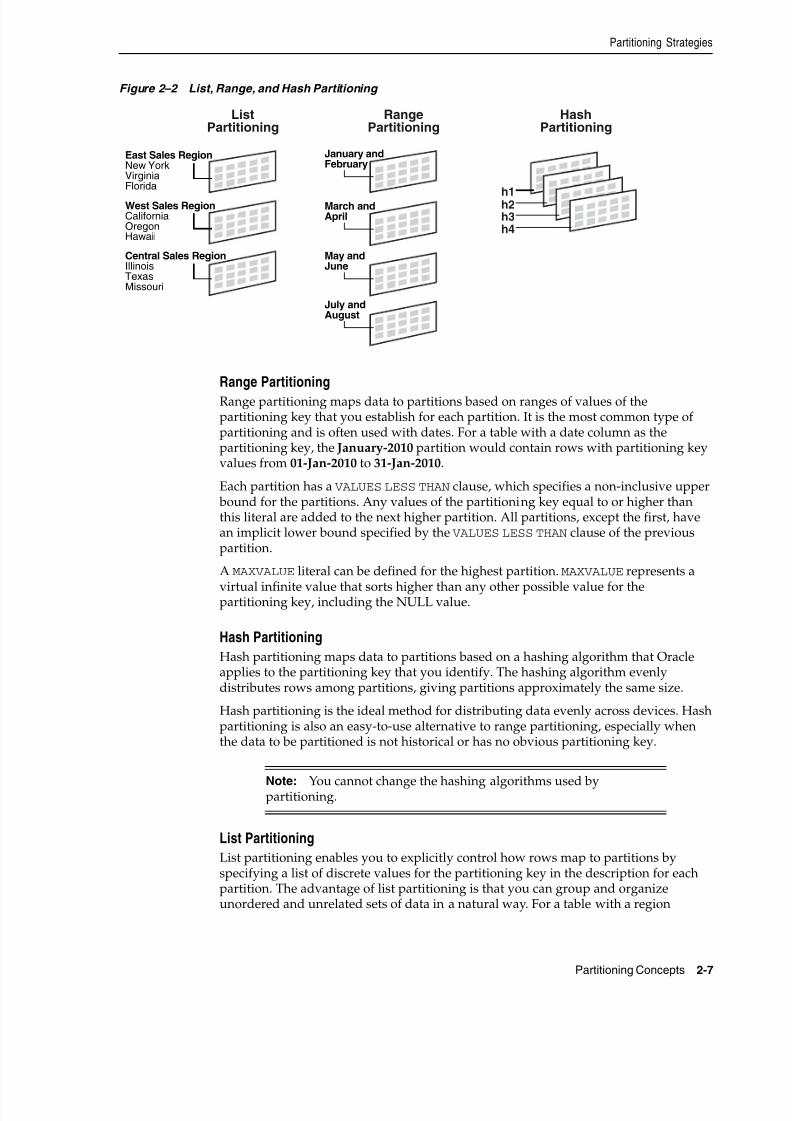
8/16/2019 Oracle Database VLDB and Partitioning Guide
http://slidepdf.com/reader/full/oracle-database-vldb-and-partitioning-guide 29/304
Partitioning Strategies
Partitioning Concepts 2-7
Figure 2–2 List, Range, and Hash Partitioning
Range Partitioning
Range partitioning maps data to partitions based on ranges of values of thepartitioning key that you establish for each partition. It is the most common type ofpartitioning and is often used with dates. For a table with a date column as thepartitioning key, the January-2010 partition would contain rows with partitioning keyvalues from 01-Jan-2010 to 31-Jan-2010.
Each partition has a VALUES LESS THAN clause, which specifies a non-inclusive upper bound for the partitions. Any values of the partitioning key equal to or higher thanthis literal are added to the next higher partition. All partitions, except the first, havean implicit lower bound specified by the VALUES LESS THAN clause of the previouspartition.
A MAXVALUE literal can be defined for the highest partition. MAXVALUE represents a
virtual infinite value that sorts higher than any other possible value for thepartitioning key, including the NULL value.
Hash Partitioning
Hash partitioning maps data to partitions based on a hashing algorithm that Oracleapplies to the partitioning key that you identify. The hashing algorithm evenlydistributes rows among partitions, giving partitions approximately the same size.
Hash partitioning is the ideal method for distributing data evenly across devices. Hashpartitioning is also an easy-to-use alternative to range partitioning, especially whenthe data to be partitioned is not historical or has no obvious partitioning key.
List Partitioning
List partitioning enables you to explicitly control how rows map to partitions byspecifying a list of discrete values for the partitioning key in the description for eachpartition. The advantage of list partitioning is that you can group and organizeunordered and unrelated sets of data in a natural way. For a table with a region
Note: You cannot change the hashing algorithms used bypartitioning.
RangePartitioning
ListPartitioning
HashPartitioning
h1
East Sales RegionNew YorkVirginiaFlorida
West Sales RegionCaliforniaOregonHawaii
Central Sales RegionIllinoisTexasMissouri
January andFebruary
March andApril
May andJune
July andAugust
h2h3h4

8/16/2019 Oracle Database VLDB and Partitioning Guide
http://slidepdf.com/reader/full/oracle-database-vldb-and-partitioning-guide 30/304
Partitioning Strategies
2-8 Oracle Database VLDB and Partitioning Guide
column as the partitioning key, the East Sales Region partition might contain valuesNew York, Virginia, and Florida.
The DEFAULT partition enables you to avoid specifying all possible values for alist-partitioned table by using a default partition, so that all rows that do not map toany other partition do not generate an error.
Composite PartitioningComposite partitioning is a combination of the basic data distribution methods; a tableis partitioned by one data distribution method and then each partition is furthersubdivided into subpartitions using a second data distribution method. Allsubpartitions for a given partition represent a logical subset of the data.
Composite partitioning supports historical operations, such as adding new rangepartitions, but also provides higher degrees of potential partition pruning and finergranularity of data placement through subpartitioning. Figure 2–3 offers a graphicalview of range-hash and range-list composite partitioning, as an example.
Figure 2–3 Composite Partitioning
■ Composite Range-Range Partitioning
■ Composite Range-Hash Partitioning
■ Composite Range-List Partitioning
■ Composite List-Range Partitioning
■ Composite List-Hash Partitioning
■ Composite List-List Partitioning
Composite Range-Range Partitioning
Composite range-range partitioning enables logical range partitioning along twodimensions; for example, partition by order_date and range subpartition byshipping_date.
Composite Range-Hash Partitioning
Composite range-hash partitioning partitions data using the range method, and withineach partition, subpartitions it using the hash method. Composite range-hash
Composite PartitioningRange-Hash
h1h2
h3
h4
h1h2
h3h4
h2h3
h1
h4
h1h2
h3h4
March andApril
Composite PartitioningRange - List
January andFebruary
May andJune
East Sales RegionNew YorkVirginiaFlorida
West Sales RegionCaliforniaOregonHawaii
Central Sales RegionIllinoisTexasMissouri
8/16/2019 Oracle Database VLDB and Partitioning Guide
http://slidepdf.com/reader/full/oracle-database-vldb-and-partitioning-guide 31/304
Partitioning Extensions
Partitioning Concepts 2-9
partitioning provides the improved manageability of range partitioning and the dataplacement, striping, and parallelism advantages of hash partitioning.
Composite Range-List Partitioning
Composite range-list partitioning partitions data using the range method, and withineach partition, subpartitions it using the list method. Composite range-list partitioning
provides the manageability of range partitioning and the explicit control of listpartitioning for the subpartitions.
Composite List-Range Partitioning
Composite list-range partitioning enables logical range subpartitioning within a givenlist partitioning strategy; for example, list partition by country_id and rangesubpartition by order_date.
Composite List-Hash Partitioning
Composite list-hash partitioning enables hash subpartitioning of a list-partitionedobject; for example, to enable partition-wise joins.
Composite List-List PartitioningComposite list-list partitioning enables logical list partitioning along two dimensions;for example, list partition by country_id and list subpartition by sales_channel.
Partitioning ExtensionsIn addition to the basic partitioning strategies, Oracle Database provides partitioningextensions:
■ Manageability Extensions
■ Partitioning Key Extensions
Manageability ExtensionsThese extensions significantly enhance the manageability of partitioned tables:
■ Interval Partitioning
■ Partition Advisor
Interval Partitioning
Interval partitioning is an extension of range partitioning which instructs the databaseto automatically create partitions of a specified interval when data inserted into thetable exceeds all of the existing range partitions. You must specify at least one rangepartition. The range partitioning key value determines the high value of the range
partitions, which is called the transition point, and the database creates intervalpartitions for data beyond that transition point. The lower boundary of every intervalpartition is the non-inclusive upper boundary of the previous range or intervalpartition.
For example, if you create an interval partitioned table with monthly intervals and thetransition point at January 1, 2007, then the lower boundary for the January 2007interval is January 1, 2007. The lower boundary for the July 2007 interval is July 1,2007, regardless of whether the June 2007 partition was created.
When using interval partitioning, consider the following restrictions:
8/16/2019 Oracle Database VLDB and Partitioning Guide
http://slidepdf.com/reader/full/oracle-database-vldb-and-partitioning-guide 32/304
Partitioning Extensions
2-10 Oracle Database VLDB and Partitioning Guide
■ You can only specify one partitioning key column, and it must be of NUMBER orDATE type.
■ Interval partitioning is not supported for index-organized tables.
■ You cannot create a domain index on an interval-partitioned table.
You can create single-level interval partitioned tables and the following composite
partitioned tables:■ Interval-range
■ Interval-hash
■ Interval-list
Partition Advisor
The Partition Advisor is part of the SQL Access Advisor. The Partition Advisor canrecommend a partitioning strategy for a table based on a supplied workload of SQLstatements which can be supplied by the SQL Cache, a SQL Tuning set, or be defined by the user.
Partitioning Key ExtensionsThese extensions extend the flexibility in defining partitioning keys:
■ Reference Partitioning
■ Virtual Column-Based Partitioning
Reference Partitioning
Reference partitioning allows the partitioning of two tables related to one another byreferential constraints. The partitioning key is resolved through an existingparent-child relationship, enforced by enabled and active primary key and foreign keyconstraints.
The benefit of this extension is that tables with a parent-child relationship can belogically equipartitioned by inheriting the partitioning key from the parent tablewithout duplicating the key columns. The logical dependency also automaticallycascades partition maintenance operations, thus making application developmenteasier and less error-prone.
An example of reference partitioning is the Orders and OrderItems tables related toeach other by a referential constraint orderid_refconstraint. Namely,OrderItems.OrderID references Orders.OrderID. The Orders table is rangepartitioned on OrderDate. Reference partitioning on orderid_refconstraint forOrderItems leads to creation of the following partitioned table, which isequipartitioned on the Orders table, as shown in Figure 2–4 and Figure 2–5.

8/16/2019 Oracle Database VLDB and Partitioning Guide
http://slidepdf.com/reader/full/oracle-database-vldb-and-partitioning-guide 33/304
Partitioning Extensions
Partitioning Concepts 2-11
Figure 2–4 Before Reference Partitioning
Figure 2–5 With Reference Partitioning
All basic partitioning strategies are available for reference Partitioning. Intervalpartitioning cannot be used with reference partitioning.
Virtual Column-Based Partitioning
In previous releases of Oracle Database, a table could only be partitioned if thepartitioning key physically existed in the table. Virtual columns remove that restrictionand allow the partitioning key to be defined by an expression, using one or moreexisting columns of a table. The expression is stored as metadata only.
Table ORDERS
. . . . . .
Table LINEITEMS
. . . . . .
Jan 2006 Feb 2006
Jan 2006 Feb 2006
· Redundant storage of order_date
· Redundant maintenance
RANGE(order_date)
Primary Key order_idForeign Key order_id
Table ORDERS
. . . . . .
Table LINEITEMS
. . . . . .
Jan 2006 Feb 2006
Jan 2006 Feb 2006
PARTITION BY REFERENCE
· Partitioning key inherited throughPK-FK relationship
RANGE(order_date)
Primary Key order_id
Foreign Key order_id
8/16/2019 Oracle Database VLDB and Partitioning Guide
http://slidepdf.com/reader/full/oracle-database-vldb-and-partitioning-guide 34/304
Overview of Partitioned Indexes
2-12 Oracle Database VLDB and Partitioning Guide
Oracle Partitioning has been enhanced to allow a partitioning strategy to be defined onvirtual columns. For example, a 10 digit account ID can include account branchinformation as the leading 3 digits. With the extension of virtual column basedPartitioning, an ACCOUNTS table containing an ACCOUNT_ID column can be extendedwith a virtual (derived) column ACCOUNT_BRANCH that is derived from the first threedigits of the ACCOUNT_ID column, which becomes the partitioning key for this table.
Virtual column-based partitioning is supported with all basic partitioning strategies,including reference Partitioning, and interval and interval-* composite partitioning.
Overview of Partitioned Indexes Just like partitioned tables, partitioned indexes improve manageability, availability,performance, and scalability. They can either be partitioned independently (globalindexes) or automatically linked to a table's partitioning method (local indexes). Ingeneral, you should use global indexes for OLTP applications and local indexes fordata warehousing or DSS applications. Also, whenever possible, you should try to uselocal indexes because they are easier to manage. When deciding what kind ofpartitioned index to use, you should consider the following guidelines in order:
1. If the table partitioning column is a subset of the index keys, use a local index. Ifthis is the case, you are finished. If this is not the case, continue to guideline 2.
2. If the index is unique and does not include the partitioning key columns, then usea global index. If this is the case, then you are finished. Otherwise, continue toguideline 3.
3. If your priority is manageability, use a local index. If this is the case, you arefinished. If this is not the case, continue to guideline 4.
4. If the application is an OLTP one and users need quick response times, use aglobal index. If the application is a DSS one and users are more interested inthroughput, use a local index.
For more information about partitioned indexes and how to decide which type to use,
refer to Chapter 6, "Using Partitioning in a Data Warehouse Environment" andChapter 7, "Using Partitioning in an Online Transaction Processing Environment".
Local Partitioned IndexesLocal partitioned indexes are easier to manage than other types of partitioned indexes.They also offer greater availability and are common in DSS environments. The reasonfor this is equipartitioning: each partition of a local index is associated with exactly onepartition of the table. This functionality enables Oracle to automatically keep the indexpartitions synchronized with the table partitions, and makes each table-index pairindependent. Any actions that make one partition's data invalid or unavailable onlyaffect a single partition.
Local partitioned indexes support more availability when there are partition orsubpartition maintenance operations on the table. A type of index called a localnonprefixed index is very useful for historical databases. In this type of index, thepartitioning is not on the left prefix of the index columns. For more information aboutprefixed indexes, refer to Chapter 3, "Partitioning for Availability, Manageability, andPerformance".
You cannot explicitly add a partition to a local index. Instead, new partitions are addedto local indexes only when you add a partition to the underlying table. Likewise, youcannot explicitly drop a partition from a local index. Instead, local index partitions aredropped only when you drop a partition from the underlying table.
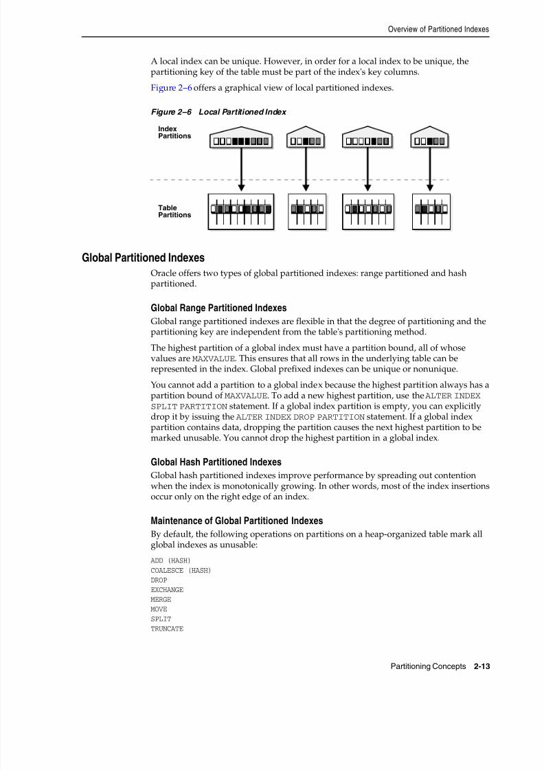
8/16/2019 Oracle Database VLDB and Partitioning Guide
http://slidepdf.com/reader/full/oracle-database-vldb-and-partitioning-guide 35/304
Overview of Partitioned Indexes
Partitioning Concepts 2-13
A local index can be unique. However, in order for a local index to be unique, thepartitioning key of the table must be part of the index's key columns.
Figure 2–6 offers a graphical view of local partitioned indexes.
Figure 2–6 Local Partitioned Index
Global Partitioned IndexesOracle offers two types of global partitioned indexes: range partitioned and hashpartitioned.
Global Range Partitioned Indexes
Global range partitioned indexes are flexible in that the degree of partitioning and thepartitioning key are independent from the table's partitioning method.
The highest partition of a global index must have a partition bound, all of whosevalues are MAXVALUE. This ensures that all rows in the underlying table can berepresented in the index. Global prefixed indexes can be unique or nonunique.
You cannot add a partition to a global index because the highest partition always has apartition bound of MAXVALUE. To add a new highest partition, use the ALTER INDEX
SPLIT PARTITION statement. If a global index partition is empty, you can explicitlydrop it by issuing the ALTER INDEX DROP PARTITION statement. If a global indexpartition contains data, dropping the partition causes the next highest partition to bemarked unusable. You cannot drop the highest partition in a global index.
Global Hash Partitioned Indexes
Global hash partitioned indexes improve performance by spreading out contentionwhen the index is monotonically growing. In other words, most of the index insertionsoccur only on the right edge of an index.
Maintenance of Global Partitioned Indexes
By default, the following operations on partitions on a heap-organized table mark allglobal indexes as unusable:
ADD (HASH)COALESCE (HASH)DROPEXCHANGEMERGEMOVESPLITTRUNCATE
Index
Partitions
TablePartitions
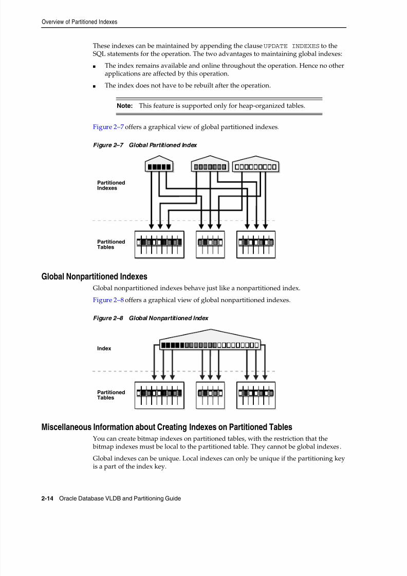
8/16/2019 Oracle Database VLDB and Partitioning Guide
http://slidepdf.com/reader/full/oracle-database-vldb-and-partitioning-guide 36/304
Overview of Partitioned Indexes
2-14 Oracle Database VLDB and Partitioning Guide
These indexes can be maintained by appending the clause UPDATE INDEXES to theSQL statements for the operation. The two advantages to maintaining global indexes:
■ The index remains available and online throughout the operation. Hence no otherapplications are affected by this operation.
■ The index does not have to be rebuilt after the operation.
Figure 2–7 offers a graphical view of global partitioned indexes.
Figure 2–7 Global Partitioned Index
Global Nonpartitioned IndexesGlobal nonpartitioned indexes behave just like a nonpartitioned index.
Figure 2–8 offers a graphical view of global nonpartitioned indexes.
Figure 2–8 Global Nonpartitioned Index
Miscellaneous Information about Creating Indexes on Partitioned TablesYou can create bitmap indexes on partitioned tables, with the restriction that the bitmap indexes must be local to the partitioned table. They cannot be global indexes.
Global indexes can be unique. Local indexes can only be unique if the partitioning keyis a part of the index key.
Note: This feature is supported only for heap-organized tables.
PartitionedIndexes
PartitionedTables
Index
PartitionedTables
8/16/2019 Oracle Database VLDB and Partitioning Guide
http://slidepdf.com/reader/full/oracle-database-vldb-and-partitioning-guide 37/304
Overview of Partitioned Indexes
Partitioning Concepts 2-15
Partitioned Indexes on Composite PartitionsHere are a few points to remember when using partitioned indexes on compositepartitions:
■ Subpartitioned indexes are always local and stored with the table subpartition bydefault.
■
Tablespaces can be specified at either index or index subpartition levels.

8/16/2019 Oracle Database VLDB and Partitioning Guide
http://slidepdf.com/reader/full/oracle-database-vldb-and-partitioning-guide 38/304
Overview of Partitioned Indexes
2-16 Oracle Database VLDB and Partitioning Guide
8/16/2019 Oracle Database VLDB and Partitioning Guide
http://slidepdf.com/reader/full/oracle-database-vldb-and-partitioning-guide 39/304
3
Partitioning for Availability, Manageability, and Performance 3-1
3Partitioning for Availability, Manageability,and Performance
This chapter provides high-level insight into how partitioning enables availability,manageability, and performance. This chapter presents guidelines on when to use agiven partitioning strategy. The main focus of this chapter is the use of tablepartitioning, though most of the recommendations and considerations apply to index
partitioning as well.This chapter contains the following topics:
■ Partition Pruning
■ Partition-Wise Joins
■ Index Partitioning
■ Partitioning and Table Compression
■ Recommendations for Choosing a Partitioning Strategy
Partition PruningPartition pruning is an essential performance feature for data warehouses. In partitionpruning, the optimizer analyzes FROM and WHERE clauses in SQL statements toeliminate unneeded partitions when building the partition access list. Thisfunctionality enables Oracle Database to perform operations only on those partitionsthat are relevant to the SQL statement.
Partition pruning dramatically reduces the amount of data retrieved from disk andshortens processing time, thus improving query performance and optimizing resourceutilization. If you partition the index and table on different columns (with a globalpartitioned index), then partition pruning also eliminates index partitions even whenthe partitions of the underlying table cannot be eliminated.
Depending upon the actual SQL statement, Oracle Database may use static or dynamic
pruning. Static pruning occurs at compile-time, with the information about thepartitions accessed beforehand while dynamic pruning occurs at run-time, meaningthat the exact partitions to be accessed by a statement are not known beforehand. Asample scenario for static pruning would be a SQL statement containing a WHERE condition with a constant literal on the partition key column. An example of dynamicpruning is the use of operators or functions in the WHERE condition.
Partition pruning affects the statistics of the objects where pruning occurs and alsoaffects the execution plan of a statement.
8/16/2019 Oracle Database VLDB and Partitioning Guide
http://slidepdf.com/reader/full/oracle-database-vldb-and-partitioning-guide 40/304
Partition Pruning
3-2 Oracle Database VLDB and Partitioning Guide
Information That Can Be Used for Partition PruningOracle Database prunes partitions when you use range, LIKE, equality, and IN-listpredicates on the range or list partitioning columns, and when you use equality andIN-list predicates on the hash partitioning columns.
On composite partitioned objects, Oracle Database can prune at both levels using therelevant predicates. Examine the table sales_range_hash, which is partitioned by
range on the column s_saledate and subpartitioned by hash on the column s_productid, and consider the following example:
Example 3–1 Creating a table with partition pruning
CREATE TABLE sales_range_hash( s_productid NUMBER, s_saledate DATE, s_custid NUMBER, s_totalprice NUMBER)PARTITION BY RANGE (s_saledate)SUBPARTITION BY HASH (s_productid) SUBPARTITIONS 8 (PARTITION sal99q1 VALUES LESS THAN (TO_DATE('01-APR-1999', 'DD-MON-YYYY')),
PARTITION sal99q2 VALUES LESS THAN (TO_DATE('01-JUL-1999', 'DD-MON-YYYY')), PARTITION sal99q3 VALUES LESS THAN (TO_DATE('01-OCT-1999', 'DD-MON-YYYY')), PARTITION sal99q4 VALUES LESS THAN (TO_DATE('01-JAN-2000', 'DD-MON-YYYY')));
SELECT * FROM sales_range_hash WHERE s_saledate BETWEEN (TO_DATE('01-JUL-1999', 'DD-MON-YYYY')) AND (TO_DATE('01-OCT-1999', 'DD-MON-YYYY')) AND s_productid = 1200;
Oracle uses the predicate on the partitioning columns to perform partition pruning asfollows:
■ When using range partitioning, Oracle accesses only partitions sal99q2 andsal99q3, representing the partitions for the third and fourth quarters of 1999.
■ When using hash subpartitioning, Oracle accesses only the one subpartition ineach partition that stores the rows with s_productid=1200. The mapping between the subpartition and the predicate is calculated based on Oracle's internalhash distribution function.
A reference-partitioned table can take advantage of partition pruning through the joinwith the referenced table. Virtual column-based partitioned tables benefit frompartition pruning for statements that use the virtual column-defining expression in theSQL statement.
How to Identify Whether Partition Pruning has been UsedWhether Oracle uses partition pruning or not is reflected in the execution plan of astatement, either in the plan table for the EXPLAIN PLAN statement or in the sharedSQL area.
The partition pruning information is reflected in the plan columns PSTART (PARTITION_START) and PSTOP (PARTITION_STOP). For serial statements, thepruning information is also reflected in the OPERATION and OPTIONS columns.
8/16/2019 Oracle Database VLDB and Partitioning Guide
http://slidepdf.com/reader/full/oracle-database-vldb-and-partitioning-guide 41/304
Partition Pruning
Partitioning for Availability, Manageability, and Performance 3-3
Static Partition PruningFor many cases, Oracle determines the partitions to be accessed at compile time. Staticpartition pruning occurs if you use static predicates, except for the following cases:
■ Partition pruning occurs using the result of a subquery.
■ The optimizer rewrites the query with a star transformation and pruning occursafter the star transformation.
■ The most efficient execution plan is a nested loop.
These three cases result in the use of dynamic pruning.
If at parse time Oracle can identify which contiguous set of partitions are accessed,then the PSTART and PSTOP columns in the execution plan show the begin and theend values of the partitions being accessed. Any other cases of partition pruning,including dynamic pruning, show the KEY value in PSTART and PSTOP, optionallywith an additional attribute.
The following is an example:
SQL> explain plan for select * from sales where time_id = to_date('01-jan-2001', 'dd-mon-yyyy');Explained.
SQL> select * from table(dbms_xplan.display);PLAN_TABLE_OUTPUT----------------------------------------------------------------------------------------------Plan hash value: 3971874201----------------------------------------------------------------------------------------------| Id | Operation | Name | Rows | Bytes | Cost (%CPU)| Time | Pstart| Pstop |----------------------------------------------------------------------------------------------| 0 | SELECT STATEMENT | | 673 | 19517 | 27 (8)| 00:00:01 | | || 1 | PARTITION RANGE SINGLE| | 673 | 19517 | 27 (8)| 00:00:01 | 17 | 17 |
|* 2 | TABLE ACCESS FULL | SALES | 673 | 19517 | 27 (8)| 00:00:01 | 17 | 17 |----------------------------------------------------------------------------------------------Predicate Information (identified by operation id):---------------------------------------------------
2 - filter("TIME_ID"=TO_DATE('2001-01-01 00:00:00', 'yyyy-mm-dd hh24:mi:ss'))
This plan shows that Oracle accesses partition number 17, as shown in the PSTART and PSTOP columns. The OPERATION column shows PARTITION RANGE SINGLE,indicating that only a single partition is being accessed. If OPERATION showsPARTITION RANGE ALL, then all partitions are being accessed and effectively nopruning takes place. PSTART then shows the very first partition of the table andPSTOP shows the very last partition.
An execution plan with a full table scan on an interval-partitioned table shows 1 for
PSTART, and 1048575 for PSTOP, regardless of how many interval partitions werecreated.
Dynamic Partition PruningDynamic pruning occurs if pruning is possible and static pruning is not possible. Thefollowing examples show multiple dynamic pruning cases.
See Also: Oracle Database Performance Tuning Guide for moreinformation about EXPLAIN PLAN and how to interpret it
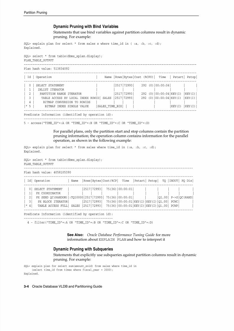
8/16/2019 Oracle Database VLDB and Partitioning Guide
http://slidepdf.com/reader/full/oracle-database-vldb-and-partitioning-guide 42/304
Partition Pruning
3-4 Oracle Database VLDB and Partitioning Guide
Dynamic Pruning with Bind Variables
Statements that use bind variables against partition columns result in dynamicpruning. For example:
SQL> explain plan for select * from sales s where time_id in ( :a, :b, :c, :d);Explained.
SQL> select * from table(dbms_xplan.display);PLAN_TABLE_OUTPUT---------------------------------------------------------------------------------------------------Plan hash value: 513834092---------------------------------------------------------------------------------------------------| Id | Operation | Name |Rows|Bytes|Cost (%CPU)| Time | Pstart| Pstop|---------------------------------------------------------------------------------------------------| 0 | SELECT STATEMENT | |2517|72993| 292 (0)|00:00:04| | || 1 | INLIST ITERATOR | | | | | | | || 2 | PARTITION RANGE ITERATOR | |2517|72993| 292 (0)|00:00:04|KEY(I) |KEY(I)|| 3 | TABLE ACCESS BY LOCAL INDEX ROWID| SALES |2517|72993| 292 (0)|00:00:04|KEY(I) |KEY(I)|| 4 | BITMAP CONVERSION TO ROWIDS | | | | | | | ||* 5 | BITMAP INDEX SINGLE VALUE |SALES_TIME_BIX| | | | |KEY(I) |KEY(I)|---------------------------------------------------------------------------------------------------
Predicate Information (identified by operation id):---------------------------------------------------5 - access("TIME_ID"=:A OR "TIME_ID"=:B OR "TIME_ID"=:C OR "TIME_ID"=:D)
For parallel plans, only the partition start and stop columns contain the partitionpruning information; the operation column contains information for the paralleloperation, as shown in the following example:
SQL> explain plan for select * from sales where time_id in (:a, :b, :c, :d);Explained.
SQL> select * from table(dbms_xplan.display);PLAN_TABLE_OUTPUT-------------------------------------------------------------------------------------------------
Plan hash value: 4058105390-------------------------------------------------------------------------------------------------| Id| Operation | Name |Rows|Bytes|Cost(%CP| Time |Pstart| Pstop| TQ |INOUT| PQ Dis|-------------------------------------------------------------------------------------------------| 0| SELECT STATEMENT | |2517|72993| 75(36)|00:00:01| | | | | || 1| PX COORDINATOR | | | | | | | | | | || 2| PX SEND QC(RANDOM)|:TQ10000|2517|72993| 75(36)|00:00:01| | |Q1,00| P->S|QC(RAND|| 3| PX BLOCK ITERATOR| |2517|72993| 75(36)|00:00:01|KEY(I)|KEY(I)|Q1,00| PCWC| ||* 4| TABLE ACCESS FULL| SALES |2517|72993| 75(36)|00:00:01|KEY(I)|KEY(I)|Q1,00| PCWP| |-------------------------------------------------------------------------------------------------Predicate Information (identified by operation id):---------------------------------------------------4 - filter("TIME_ID"=:A OR "TIME_ID"=:B OR "TIME_ID"=:C OR "TIME_ID"=:D)
Dynamic Pruning with Subqueries
Statements that explicitly use subqueries against partition columns result in dynamicpruning. For example:
SQL> explain plan for select sum(amount_sold) from sales where time_id in (select time_id from times where fiscal_year = 2000);
Explained.
See Also: Oracle Database Performance Tuning Guide for moreinformation about EXPLAIN PLAN and how to interpret it
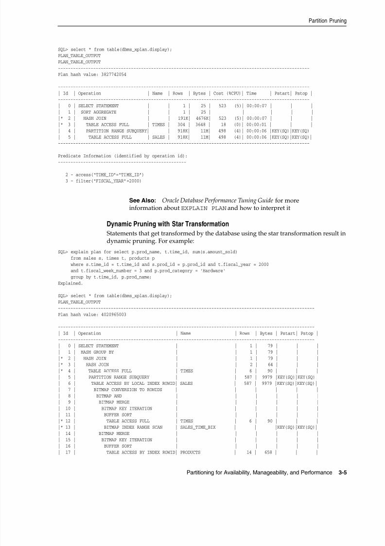
8/16/2019 Oracle Database VLDB and Partitioning Guide
http://slidepdf.com/reader/full/oracle-database-vldb-and-partitioning-guide 43/304
Partition Pruning
Partitioning for Availability, Manageability, and Performance 3-5
SQL> select * from table(dbms_xplan.display);PLAN_TABLE_OUTPUT
PLAN_TABLE_OUTPUT
----------------------------------------------------------------------------------------------------Plan hash value: 3827742054
----------------------------------------------------------------------------------------------------
| Id | Operation | Name | Rows | Bytes | Cost (%CPU)| Time | Pstart| Pstop |----------------------------------------------------------------------------------------------------
| 0 | SELECT STATEMENT | | 1 | 25 | 523 (5)| 00:00:07 | | |
| 1 | SORT AGGREGATE | | 1 | 25 | | | | ||* 2 | HASH JOIN | | 191K| 4676K| 523 (5)| 00:00:07 | | |
|* 3 | TABLE ACCESS FULL | TIMES | 304 | 3648 | 18 (0)| 00:00:01 | | |
| 4 | PARTITION RANGE SUBQUERY| | 918K| 11M| 498 (4)| 00:00:06 |KEY(SQ)|KEY(SQ)|
| 5 | TABLE ACCESS FULL | SALES | 918K| 11M| 498 (4)| 00:00:06 |KEY(SQ)|KEY(SQ)|----------------------------------------------------------------------------------------------------
Predicate Information (identified by operation id):---------------------------------------------------
2 - access("TIME_ID"="TIME_ID") 3 - filter("FISCAL_YEAR"=2000)
Dynamic Pruning with Star Transformation
Statements that get transformed by the database using the star transformation result indynamic pruning. For example:
SQL> explain plan for select p.prod_name, t.time_id, sum(s.amount_sold)
from sales s, times t, products p
where s.time_id = t.time_id and s.prod_id = p.prod_id and t.fiscal_year = 2000 and t.fiscal_week_number = 3 and p.prod_category = 'Hardware'
group by t.time_id, p.prod_name;
Explained.
SQL> select * from table(dbms_xplan.display);
PLAN_TABLE_OUTPUT------------------------------------------------------------------------------------------------------
Plan hash value: 4020965003
------------------------------------------------------------------------------------------------------
| Id | Operation | Name | Rows | Bytes | Pstart| Pstop |
------------------------------------------------------------------------------------------------------| 0 | SELECT STATEMENT | | 1 | 79 | | |
| 1 | HASH GROUP BY | | 1 | 79 | | |
|* 2 | HASH JOIN | | 1 | 79 | | ||* 3 | HASH JOIN | | 2 | 64 | | |
|* 4 | TABLE ACCESS FULL | TIMES | 6 | 90 | | |
| 5 | PARTITION RANGE SUBQUERY | | 587 | 9979 |KEY(SQ)|KEY(SQ)|
| 6 | TABLE ACCESS BY LOCAL INDEX ROWID| SALES | 587 | 9979 |KEY(SQ)|KEY(SQ)|| 7 | BITMAP CONVERSION TO ROWIDS | | | | | |
| 8 | BITMAP AND | | | | | || 9 | BITMAP MERGE | | | | | |
| 10 | BITMAP KEY ITERATION | | | | | |
| 11 | BUFFER SORT | | | | | |
|* 12 | TABLE ACCESS FULL | TIMES | 6 | 90 | | ||* 13 | BITMAP INDEX RANGE SCAN | SALES_TIME_BIX | | |KEY(SQ)|KEY(SQ)|
| 14 | BITMAP MERGE | | | | | |
| 15 | BITMAP KEY ITERATION | | | | | || 16 | BUFFER SORT | | | | | |
| 17 | TABLE ACCESS BY INDEX ROWID| PRODUCTS | 14 | 658 | | |
See Also: Oracle Database Performance Tuning Guide for moreinformation about EXPLAIN PLAN and how to interpret it
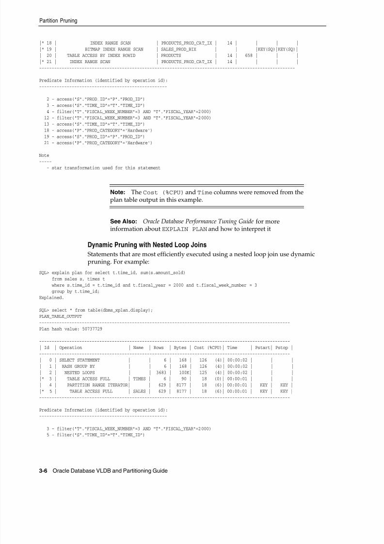
8/16/2019 Oracle Database VLDB and Partitioning Guide
http://slidepdf.com/reader/full/oracle-database-vldb-and-partitioning-guide 44/304
Partition Pruning
3-6 Oracle Database VLDB and Partitioning Guide
|* 18 | INDEX RANGE SCAN | PRODUCTS_PROD_CAT_IX | 14 | | | |
|* 19 | BITMAP INDEX RANGE SCAN | SALES_PROD_BIX | | |KEY(SQ)|KEY(SQ)|| 20 | TABLE ACCESS BY INDEX ROWID | PRODUCTS | 14 | 658 | | |
|* 21 | INDEX RANGE SCAN | PRODUCTS_PROD_CAT_IX | 14 | | | |
------------------------------------------------------------------------------------------------------
Predicate Information (identified by operation id):
---------------------------------------------------
2 - access("S"."PROD_ID"="P"."PROD_ID")
3 - access("S"."TIME_ID"="T"."TIME_ID")
4 - filter("T"."FISCAL_WEEK_NUMBER"=3 AND "T"."FISCAL_YEAR"=2000) 12 - filter("T"."FISCAL_WEEK_NUMBER"=3 AND "T"."FISCAL_YEAR"=2000)
13 - access("S"."TIME_ID"="T"."TIME_ID")
18 - access("P"."PROD_CATEGORY"='Hardware')
19 - access("S"."PROD_ID"="P"."PROD_ID") 21 - access("P"."PROD_CATEGORY"='Hardware')
Note-----
- star transformation used for this statement
Dynamic Pruning with Nested Loop Joins
Statements that are most efficiently executed using a nested loop join use dynamicpruning. For example:
SQL> explain plan for select t.time_id, sum(s.amount_sold)
from sales s, times t
where s.time_id = t.time_id and t.fiscal_year = 2000 and t.fiscal_week_number = 3 group by t.time_id;
Explained.
SQL> select * from table(dbms_xplan.display);PLAN_TABLE_OUTPUT
----------------------------------------------------------------------------------------------------
Plan hash value: 50737729
----------------------------------------------------------------------------------------------------
| Id | Operation | Name | Rows | Bytes | Cost (%CPU)| Time | Pstart| Pstop |----------------------------------------------------------------------------------------------------
| 0 | SELECT STATEMENT | | 6 | 168 | 126 (4)| 00:00:02 | | |
| 1 | HASH GROUP BY | | 6 | 168 | 126 (4)| 00:00:02 | | |
| 2 | NESTED LOOPS | | 3683 | 100K| 125 (4)| 00:00:02 | | |
|* 3 | TABLE ACCESS FULL | TIMES | 6 | 90 | 18 (0)| 00:00:01 | | || 4 | PARTITION RANGE ITERATOR| | 629 | 8177 | 18 (6)| 00:00:01 | KEY | KEY |
|* 5 | TABLE ACCESS FULL | SALES | 629 | 8177 | 18 (6)| 00:00:01 | KEY | KEY |----------------------------------------------------------------------------------------------------
Predicate Information (identified by operation id):---------------------------------------------------
3 - filter("T"."FISCAL_WEEK_NUMBER"=3 AND "T"."FISCAL_YEAR"=2000) 5 - filter("S"."TIME_ID"="T"."TIME_ID")
Note: The Cost (%CPU) and Time columns were removed from theplan table output in this example.
See Also: Oracle Database Performance Tuning Guide for moreinformation about EXPLAIN PLAN and how to interpret it
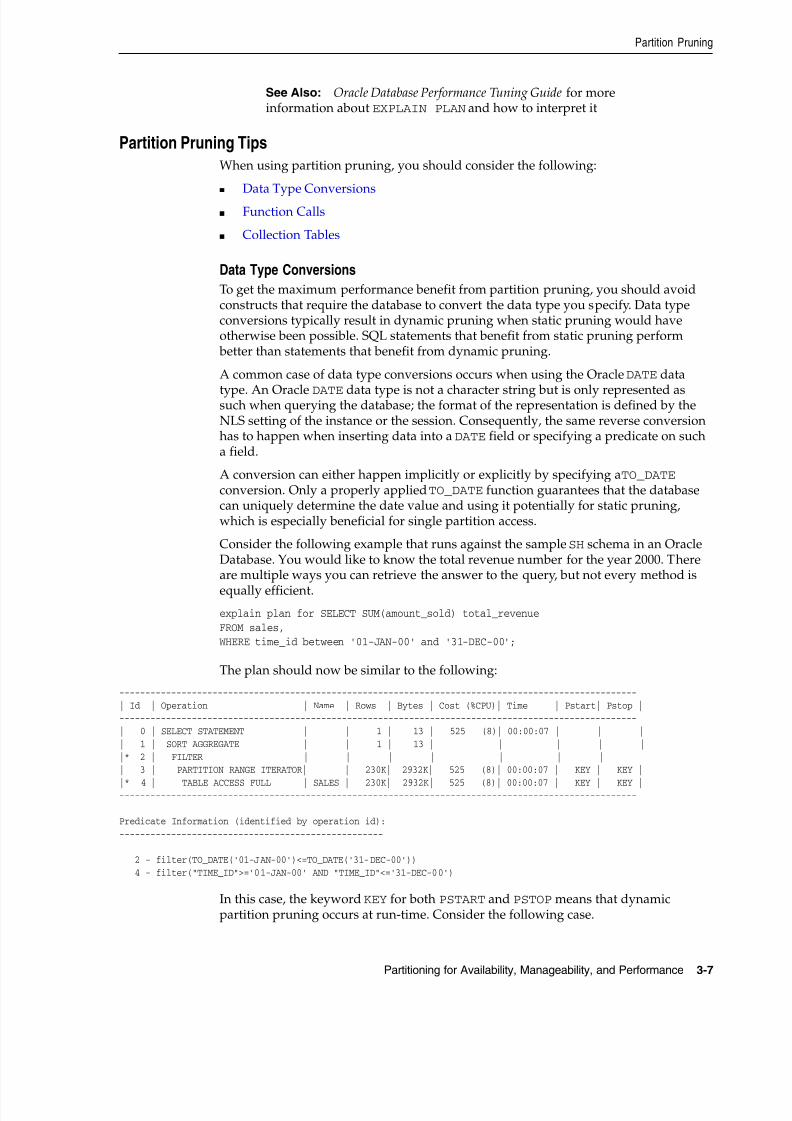
8/16/2019 Oracle Database VLDB and Partitioning Guide
http://slidepdf.com/reader/full/oracle-database-vldb-and-partitioning-guide 45/304
Partition Pruning
Partitioning for Availability, Manageability, and Performance 3-7
Partition Pruning TipsWhen using partition pruning, you should consider the following:
■ Data Type Conversions
■ Function Calls
■ Collection Tables
Data Type Conversions
To get the maximum performance benefit from partition pruning, you should avoidconstructs that require the database to convert the data type you specify. Data typeconversions typically result in dynamic pruning when static pruning would haveotherwise been possible. SQL statements that benefit from static pruning perform better than statements that benefit from dynamic pruning.
A common case of data type conversions occurs when using the Oracle DATE data
type. An Oracle DATE data type is not a character string but is only represented assuch when querying the database; the format of the representation is defined by theNLS setting of the instance or the session. Consequently, the same reverse conversionhas to happen when inserting data into a DATE field or specifying a predicate on sucha field.
A conversion can either happen implicitly or explicitly by specifying a TO_DATE conversion. Only a properly applied TO_DATE function guarantees that the databasecan uniquely determine the date value and using it potentially for static pruning,which is especially beneficial for single partition access.
Consider the following example that runs against the sample SH schema in an OracleDatabase. You would like to know the total revenue number for the year 2000. Thereare multiple ways you can retrieve the answer to the query, but not every method is
equally efficient.
explain plan for SELECT SUM(amount_sold) total_revenueFROM sales,
WHERE time_id between '01-JAN-00' and '31-DEC-00';
The plan should now be similar to the following:
----------------------------------------------------------------------------------------------------
| Id | Operation | Name | Rows | Bytes | Cost (%CPU)| Time | Pstart| Pstop |----------------------------------------------------------------------------------------------------
| 0 | SELECT STATEMENT | | 1 | 13 | 525 (8)| 00:00:07 | | |
| 1 | SORT AGGREGATE | | 1 | 13 | | | | |
|* 2 | FILTER | | | | | | | || 3 | PARTITION RANGE ITERATOR| | 230K| 2932K| 525 (8)| 00:00:07 | KEY | KEY |
|* 4 | TABLE ACCESS FULL | SALES | 230K| 2932K| 525 (8)| 00:00:07 | KEY | KEY |----------------------------------------------------------------------------------------------------
Predicate Information (identified by operation id):
---------------------------------------------------
2 - filter(TO_DATE('01-JAN-00')<=TO_DATE('31-DEC-00'))
4 - filter("TIME_ID">='01-JAN-00' AND "TIME_ID"<='31-DEC-00')
In this case, the keyword KEY for both PSTART and PSTOP means that dynamicpartition pruning occurs at run-time. Consider the following case.
See Also: Oracle Database Performance Tuning Guide for moreinformation about EXPLAIN PLAN and how to interpret it

8/16/2019 Oracle Database VLDB and Partitioning Guide
http://slidepdf.com/reader/full/oracle-database-vldb-and-partitioning-guide 46/304
Partition Pruning
3-8 Oracle Database VLDB and Partitioning Guide
explain plan for select sum(amount_sold)from sales
where time_id between '01-JAN-2000' and '31-DEC-2000' ;
The execution plan now shows the following:
----------------------------------------------------------------------------------------| Id | Operation | Name | Rows | Bytes | Cost (%CPU)| Pstart| Pstop |
----------------------------------------------------------------------------------------| 0 | SELECT STATEMENT | | 1 | 13 | 127 (4)| | || 1 | SORT AGGREGATE | | 1 | 13 | | | || 2 | PARTITION RANGE ITERATOR| | 230K| 2932K| 127 (4)| 13 | 16 ||* 3 | TABLE ACCESS FULL | SALES | 230K| 2932K| 127 (4)| 13 | 16 |----------------------------------------------------------------------------------------Predicate Information (identified by operation id):---------------------------------------------------
3 - filter("TIME_ID"<=TO_DATE(' 2000-12-31 00:00:00', "syyyy-mm-dd hh24:mi:ss'))
The execution plan shows static partition pruning. The query accesses a contiguous listof partitions 13 to 16. In this particular case the way the date format was specifiedmatches the NLS date format setting. Though this example shows the most efficientexecution plan, you cannot rely on the NLS date format setting to define a certainformat.
alter session set nls_date_format='fmdd Month yyyy';
explain plan for select sum(amount_sold)from sales
where time_id between '01-JAN-2000' and '31-DEC-2000' ;
The execution plan now shows the following:-----------------------------------------------------------------------------------------| Id | Operation | Name | Rows | Bytes | Cost (%CPU)| Pstart| Pstop |-----------------------------------------------------------------------------------------| 0 | SELECT STATEMENT | | 1 | 13 | 525 (8)| | || 1 | SORT AGGREGATE | | 1 | 13 | | | ||* 2 | FILTER | | | | | | || 3 | PARTITION RANGE ITERATOR| | 230K| 2932K| 525 (8)| KEY | KEY ||* 4 | TABLE ACCESS FULL | SALES | 230K| 2932K| 525 (8)| KEY | KEY |-----------------------------------------------------------------------------------------
Predicate Information (identified by operation id):---------------------------------------------------
2 - filter(TO_DATE('01-JAN-2000')<=TO_DATE('31-DEC-2000')) 4 - filter("TIME_ID">='01-JAN-2000' AND "TIME_ID"<='31-DEC-2000')
Note: The Time column was removed from the execution plan.
Note: The Time column was removed from the execution plan.
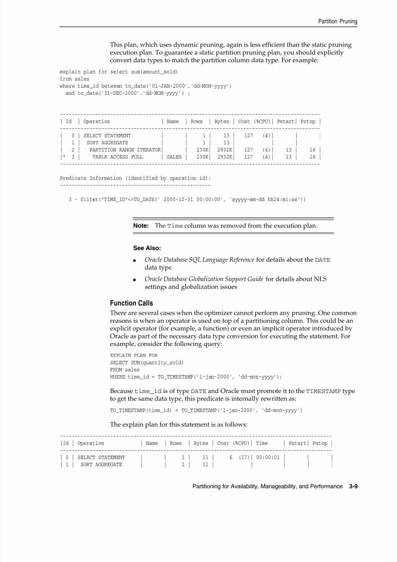
8/16/2019 Oracle Database VLDB and Partitioning Guide
http://slidepdf.com/reader/full/oracle-database-vldb-and-partitioning-guide 47/304
Partition Pruning
Partitioning for Availability, Manageability, and Performance 3-9
This plan, which uses dynamic pruning, again is less efficient than the static pruningexecution plan. To guarantee a static partition pruning plan, you should explicitlyconvert data types to match the partition column data type. For example:
explain plan for select sum(amount_sold)from sales
where time_id between to_date('01-JAN-2000','dd-MON-yyyy') and to_date('31-DEC-2000','dd-MON-yyyy') ;
----------------------------------------------------------------------------------------| Id | Operation | Name | Rows | Bytes | Cost (%CPU)| Pstart| Pstop |----------------------------------------------------------------------------------------| 0 | SELECT STATEMENT | | 1 | 13 | 127 (4)| | || 1 | SORT AGGREGATE | | 1 | 13 | | | || 2 | PARTITION RANGE ITERATOR| | 230K| 2932K| 127 (4)| 13 | 16 ||* 3 | TABLE ACCESS FULL | SALES | 230K| 2932K| 127 (4)| 13 | 16 |----------------------------------------------------------------------------------------
Predicate Information (identified by operation id):---------------------------------------------------
3 - filter("TIME_ID"<=TO_DATE(' 2000-12-31 00:00:00', 'syyyy-mm-dd hh24:mi:ss'))
Function Calls
There are several cases when the optimizer cannot perform any pruning. One commonreasons is when an operator is used on top of a partitioning column. This could be anexplicit operator (for example, a function) or even an implicit operator introduced byOracle as part of the necessary data type conversion for executing the statement. Forexample, consider the following query:
EXPLAIN PLAN FORSELECT SUM(quantity_sold)FROM sales
WHERE time_id = TO_TIMESTAMP('1-jan-2000', 'dd-mon-yyyy');
Because time_id is of type DATE and Oracle must promote it to the TIMESTAMP typeto get the same data type, this predicate is internally rewritten as:
TO_TIMESTAMP(time_id) = TO_TIMESTAMP('1-jan-2000', 'dd-mon-yyyy')
The explain plan for this statement is as follows:
--------------------------------------------------------------------------------------------|Id | Operation | Name | Rows | Bytes | Cost (%CPU)| Time | Pstart| Pstop |--------------------------------------------------------------------------------------------| 0 | SELECT STATEMENT | | 1 | 11 | 6 (17)| 00:00:01 | | || 1 | SORT AGGREGATE | | 1 | 11 | | | | |
Note: The Time column was removed from the execution plan.
See Also:
■ Oracle Database SQL Language Reference for details about the DATE data type
■ Oracle Database Globalization Support Guide for details about NLSsettings and globalization issues
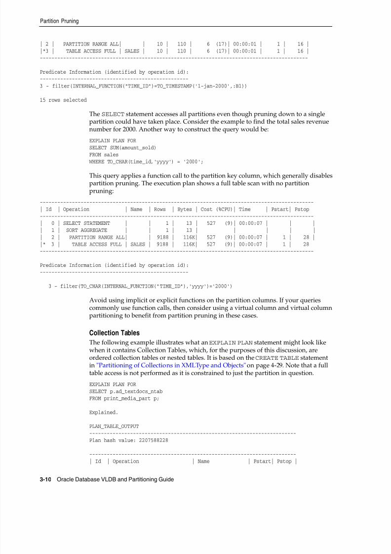
8/16/2019 Oracle Database VLDB and Partitioning Guide
http://slidepdf.com/reader/full/oracle-database-vldb-and-partitioning-guide 48/304
Partition Pruning
3-10 Oracle Database VLDB and Partitioning Guide
| 2 | PARTITION RANGE ALL| | 10 | 110 | 6 (17)| 00:00:01 | 1 | 16 ||*3 | TABLE ACCESS FULL | SALES | 10 | 110 | 6 (17)| 00:00:01 | 1 | 16 |-------------------------------------------------------------------------------------------- Predicate Information (identified by operation id):---------------------------------------------------3 - filter(INTERNAL_FUNCTION("TIME_ID")=TO_TIMESTAMP('1-jan-2000',:B1)) 15 rows selected
The SELECT statement accesses all partitions even though pruning down to a singlepartition could have taken place. Consider the example to find the total sales revenuenumber for 2000. Another way to construct the query would be:
EXPLAIN PLAN FORSELECT SUM(amount_sold)FROM sales
WHERE TO_CHAR(time_id,'yyyy') = '2000';
This query applies a function call to the partition key column, which generally disablespartition pruning. The execution plan shows a full table scan with no partition
pruning:----------------------------------------------------------------------------------------------| Id | Operation | Name | Rows | Bytes | Cost (%CPU)| Time | Pstart| Pstop |----------------------------------------------------------------------------------------------| 0 | SELECT STATEMENT | | 1 | 13 | 527 (9)| 00:00:07 | | || 1 | SORT AGGREGATE | | 1 | 13 | | | | || 2 | PARTITION RANGE ALL| | 9188 | 116K| 527 (9)| 00:00:07 | 1 | 28 ||* 3 | TABLE ACCESS FULL | SALES | 9188 | 116K| 527 (9)| 00:00:07 | 1 | 28 |----------------------------------------------------------------------------------------------
Predicate Information (identified by operation id):---------------------------------------------------
3 - filter(TO_CHAR(INTERNAL_FUNCTION("TIME_ID"),'yyyy')='2000')
Avoid using implicit or explicit functions on the partition columns. If your queriescommonly use function calls, then consider using a virtual column and virtual columnpartitioning to benefit from partition pruning in these cases.
Collection Tables
The following example illustrates what an EXPLAIN PLAN statement might look likewhen it contains Collection Tables, which, for the purposes of this discussion, areordered collection tables or nested tables. It is based on the CREATE TABLE statementin "Partitioning of Collections in XMLType and Objects" on page 4-29. Note that a fulltable access is not performed as it is constrained to just the partition in question.
EXPLAIN PLAN FORSELECT p.ad_textdocs_ntabFROM print_media_part p; Explained. PLAN_TABLE_OUTPUT-----------------------------------------------------------------------Plan hash value: 2207588228 -----------------------------------------------------------------------| Id | Operation | Name | Pstart| Pstop |

8/16/2019 Oracle Database VLDB and Partitioning Guide
http://slidepdf.com/reader/full/oracle-database-vldb-and-partitioning-guide 49/304
Partition-Wise Joins
Partitioning for Availability, Manageability, and Performance 3-11
-----------------------------------------------------------------------| 0 | SELECT STATEMENT | | | || 1 | PARTITION REFERENCE SINGLE| | KEY | KEY || 2 | TABLE ACCESS FULL | TEXTDOC_NT | KEY | KEY || 3 | PARTITION RANGE ALL | | 1 | 2 || 4 | TABLE ACCESS FULL | PRINT_MEDIA_PART | 1 | 2 |----------------------------------------------------------------------- Note----- - dynamic sampling used for this statement
Partition-Wise JoinsPartition-wise joins reduce query response time by minimizing the amount of dataexchanged among parallel execution servers when joins execute in parallel. Thissignificantly reduces response time and improves the use of both CPU and memoryresources. In Oracle Real Application Clusters (Oracle RAC) environments,partition-wise joins also avoid or at least limit the data traffic over the interconnect,which is the key to achieving good scalability for massive join operations.
Partition-wise joins can be full or partial. Oracle Database decides which type of join touse.
Full Partition-Wise JoinsA full partition-wise join divides a large join into smaller joins between a pair ofpartitions from the two joined tables. To use this feature, you must equipartition bothtables on their join keys, or use reference partitioning. For example, consider a large join between a sales table and a customer table on the column cust_id. The query"find the records of all customers who bought more than 100 articles in Quarter 3 of1999" is a typical example of a SQL statement performing such a join. The following isan example of this:
Example 3–2 Querying with a full partition-wise join
SELECT c.cust_last_name, COUNT(*) FROM sales s, customers c WHERE s.cust_id = c.cust_id AND
s.time_id BETWEEN TO_DATE('01-JUL-1999', 'DD-MON-YYYY') AND(TO_DATE('01-OCT-1999', 'DD-MON-YYYY'))
GROUP BY c.cust_last_name HAVING COUNT(*) > 100;
Such a large join is typical in data warehousing environments. In this case, the entirecustomer table is joined with one quarter of the sales data. In large data warehouseapplications, this might mean joining millions of rows. The join method to use in thatcase is obviously a hash join. You can reduce the processing time for this hash join
even more if both tables are equipartitioned on the cust_id column. Thisfunctionality enables a full partition-wise join.
When you execute a full partition-wise join in parallel, the granule of parallelism is apartition. Consequently, the degree of parallelism is limited to the number ofpartitions. For example, you require at least 16 partitions to set the degree ofparallelism of the query to 16.
You can use various partitioning methods to equipartition both tables. These methodsare described at a high level in the following subsections.
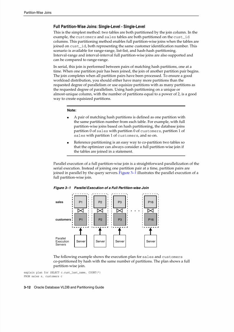
8/16/2019 Oracle Database VLDB and Partitioning Guide
http://slidepdf.com/reader/full/oracle-database-vldb-and-partitioning-guide 50/304
Partition-Wise Joins
3-12 Oracle Database VLDB and Partitioning Guide
Full Partition-Wise Joins: Single-Level - Single-Level
This is the simplest method: two tables are both partitioned by the join column. In theexample, the customers and sales tables are both partitioned on the cust_id columns. This partitioning method enables full partition-wise joins when the tables are joined on cust_id, both representing the same customer identification number. Thisscenario is available for range-range, list-list, and hash-hash partitioning.Interval-range and interval-interval full partition-wise joins are also supported andcan be compared to range-range.
In serial, this join is performed between pairs of matching hash partitions, one at atime. When one partition pair has been joined, the join of another partition pair begins.The join completes when all partition pairs have been processed. To ensure a goodworkload distribution, you should either have many more partitions than therequested degree of parallelism or use equisize partitions with as many partitions asthe requested degree of parallelism. Using hash partitioning on a unique oralmost-unique column, with the number of partitions equal to a power of 2, is a goodway to create equisized partitions.
Parallel execution of a full partition-wise join is a straightforward parallelization of theserial execution. Instead of joining one partition pair at a time, partition pairs are
joined in parallel by the query servers. Figure 3–1 illustrates the parallel execution of afull partition-wise join.
Figure 3–1 Parallel Execution of a Full Partition-wise Join
The following example shows the execution plan for sales and customers co-partitioned by hash with the same number of partitions. The plan shows a fullpartition-wise join.
explain plan for SELECT c.cust_last_name, COUNT(*)
FROM sales s, customers c
Note:
■ A pair of matching hash partitions is defined as one partition withthe same partition number from each table. For example, with fullpartition-wise joins based on hash partitioning, the database joinspartition 0 of sales with partition 0 of customers, partition 1 ofsales with partition 1 of customers, and so on.
■ Reference partitioning is an easy way to co-partition two tables sothat the optimizer can always consider a full partition-wise join ifthe tables are joined in a statement.
Server
P1
P1
Server
P2
P2
Server
P3
P3
Server
P16
P16
. . .sales
customers
ParallelExecutionServers

8/16/2019 Oracle Database VLDB and Partitioning Guide
http://slidepdf.com/reader/full/oracle-database-vldb-and-partitioning-guide 51/304
Partition-Wise Joins
Partitioning for Availability, Manageability, and Performance 3-13
WHERE s.cust_id = c.cust_id AND
s.time_id BETWEEN TO_DATE('01-JUL-1999', 'DD-MON-YYYY') AND(TO_DATE('01-OCT-1999', 'DD-MON-YYYY'))
GROUP BY c.cust_last_name HAVING COUNT(*) > 100;
---------------------------------------------------------------------------------------------------------------
| Id | Operation | Name | Rows | Bytes | Pstart| Pstop | TQ |IN-OUT| PQ Distrib |
---------------------------------------------------------------------------------------------------------------
| 0 | SELECT STATEMENT | | 46 | 1196 | | | | | || 1 | PX COORDINATOR | | | | | | | | |
| 2 | PX SEND QC (RANDOM) | :TQ10001 | 46 | 1196 | | | Q1,01 | P->S | QC (RAND) |
|* 3 | FILTER | | | | | | Q1,01 | PCWC | || 4 | HASH GROUP BY | | 46 | 1196 | | | Q1,01 | PCWP | |
| 5 | PX RECEIVE | | 46 | 1196 | | | Q1,01 | PCWP | |
| 6 | PX SEND HASH | :TQ10000 | 46 | 1196 | | | Q1,00 | P->P | HASH |
| 7 | HASH GROUP BY | | 46 | 1196 | | | Q1,00 | PCWP | || 8 | PX PARTITION HASH ALL| | 59158 | 1502K| 1 | 16 | Q1,00 | PCWC | |
|* 9 | HASH JOIN | | 59158 | 1502K| | | Q1,00 | PCWP | |
| 10 | TABLE ACCESS FULL | CUSTOMERS | 55500 | 704K| 1 | 16 | Q1,00 | PCWP | ||* 11 | TABLE ACCESS FULL | SALES | 59158 | 751K| 1 | 16 | Q1,00 | PCWP | |
---------------------------------------------------------------------------------------------------------------
Predicate Information (identified by operation id):
---------------------------------------------------
3 - filter(COUNT(SYS_OP_CSR(SYS_OP_MSR(COUNT(*)),0))>100)
9 - access("S"."CUST_ID"="C"."CUST_ID")
11 - filter("S"."TIME_ID"<=TO_DATE(' 1999-10-01 00:00:00', 'syyyy-mm-dd hh24:mi:ss') AND
"S"."TIME_ID">=TO_DATE(' 1999-07-01 00:00:00', 'syyyy-mm-dd hh24:mi:ss'))
In Oracle Real Application Clusters environments running on MPP platforms, placing
partitions on nodes is critical to achieving good scalability. To avoid remote I/O, bothmatching partitions should have affinity to the same node. Partition pairs should bespread over all nodes to avoid bottlenecks and to use all CPU resources available onthe system.
Nodes can host multiple pairs when there are more pairs than nodes. For example,with an 8-node system and 16 partition pairs, each node receives two pairs.
Full Partition-Wise Joins: Composite - Single-Level
This method is a variation of the single-level - single-level method. In this scenario,
one table (typically the larger table) is composite partitioned on two dimensions, usingthe join columns as the subpartition key. In the example, the sales table is a typicalexample of a table storing historical data. Using range partitioning is a logical initialpartitioning method for a table storing historical information.
For example, assume you want to partition the sales table into eight partitions byrange on the column time_id. Also assume you have two years and that eachpartition represents a quarter. Instead of using range partitioning, you can usecomposite partitioning to enable a full partition-wise join while preserving thepartitioning on time_id. For example, partition the sales table by range on time_id and then subpartition each partition by hash on cust_id using 16 subpartitions
Note: The Cost (%CPU) and Time columns were removed from theplan table output in this example.
See Also: Oracle Real Application Clusters Administration andDeployment Guide for more information about data affinity

8/16/2019 Oracle Database VLDB and Partitioning Guide
http://slidepdf.com/reader/full/oracle-database-vldb-and-partitioning-guide 52/304
Partition-Wise Joins
3-14 Oracle Database VLDB and Partitioning Guide
for each partition, for a total of 128 subpartitions. The customers table can use hashpartitioning with 16 partitions.
When you use the method just described, a full partition-wise join works similarly tothe one created by a single-level - single-level hash-hash method. The join is stilldivided into 16 smaller joins between hash partition pairs from both tables. Thedifference is that now each hash partition in the sales table is composed of a set of 8
subpartitions, one from each range partition.Figure 3–2 illustrates how the hash partitions are formed in the sales table. Each cellrepresents a subpartition. Each row corresponds to one range partition, for a total of 8range partitions. Each range partition has 16 subpartitions. Each column correspondsto one hash partition for a total of 16 hash partitions; each hash partition has 8subpartitions. Note that hash partitions can be defined only if all partitions have thesame number of subpartitions, in this case, 16.
Hash partitions are implicit in a composite table. However, Oracle does not recordthem in the data dictionary, and you cannot manipulate them with DDL commands asyou can range or list partitions.
Figure 3–2 Range and Hash Partitions of a Composite Table
The following example shows the execution plan for the full partition-wise join withthe sales table range partitioned by time_id, and subpartitioned by hash on cust_id.
----------------------------------------------------------------------------------------------| Id | Operation | Name | Pstart| Pstop |IN-OUT| PQ Distrib |----------------------------------------------------------------------------------------------| 0 | SELECT STATEMENT | | | | | || 1 | PX COORDINATOR | | | | | |
1999 - Q1
1999 - Q2
1999 - Q3
1999 - Q4
2000 - Q1
2000 - Q2
2000 - Q3
2000 - Q4
Hash partition #9
H1
H2
H3
H4
H5
H6
H7
H8
H9
H10
H11
H12
H13
H14
H15
H16
s a l e s d a t e
customerid
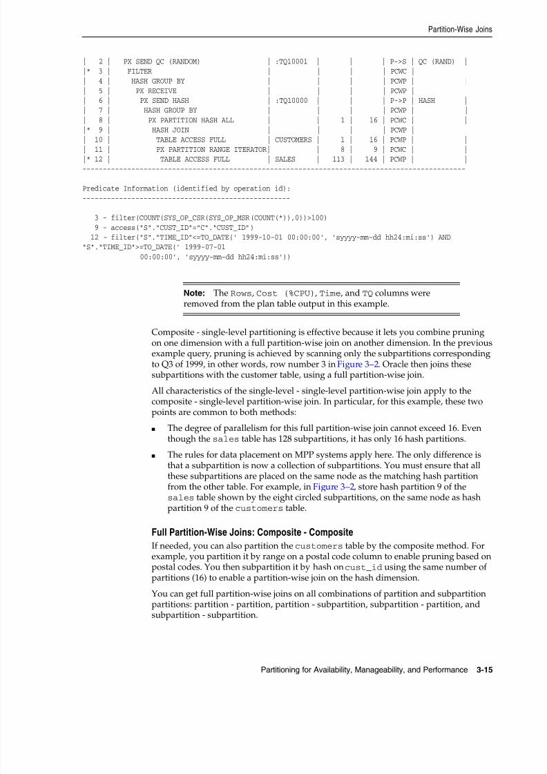
8/16/2019 Oracle Database VLDB and Partitioning Guide
http://slidepdf.com/reader/full/oracle-database-vldb-and-partitioning-guide 53/304
Partition-Wise Joins
Partitioning for Availability, Manageability, and Performance 3-15
| 2 | PX SEND QC (RANDOM) | :TQ10001 | | | P->S | QC (RAND) ||* 3 | FILTER | | | | PCWC | || 4 | HASH GROUP BY | | | | PCWP | || 5 | PX RECEIVE | | | | PCWP | || 6 | PX SEND HASH | :TQ10000 | | | P->P | HASH || 7 | HASH GROUP BY | | | | PCWP | || 8 | PX PARTITION HASH ALL | | 1 | 16 | PCWC | ||* 9 | HASH JOIN | | | | PCWP | || 10 | TABLE ACCESS FULL | CUSTOMERS | 1 | 16 | PCWP | || 11 | PX PARTITION RANGE ITERATOR| | 8 | 9 | PCWC | ||* 12 | TABLE ACCESS FULL | SALES | 113 | 144 | PCWP | |----------------------------------------------------------------------------------------------
Predicate Information (identified by operation id):---------------------------------------------------
3 - filter(COUNT(SYS_OP_CSR(SYS_OP_MSR(COUNT(*)),0))>100) 9 - access("S"."CUST_ID"="C"."CUST_ID") 12 - filter("S"."TIME_ID"<=TO_DATE(' 1999-10-01 00:00:00', 'syyyy-mm-dd hh24:mi:ss') AND"S"."TIME_ID">=TO_DATE(' 1999-07-01 00:00:00', 'syyyy-mm-dd hh24:mi:ss'))
Composite - single-level partitioning is effective because it lets you combine pruningon one dimension with a full partition-wise join on another dimension. In the previousexample query, pruning is achieved by scanning only the subpartitions correspondingto Q3 of 1999, in other words, row number 3 in Figure 3–2. Oracle then joins thesesubpartitions with the customer table, using a full partition-wise join.
All characteristics of the single-level - single-level partition-wise join apply to thecomposite - single-level partition-wise join. In particular, for this example, these twopoints are common to both methods:
■ The degree of parallelism for this full partition-wise join cannot exceed 16. Eventhough the sales table has 128 subpartitions, it has only 16 hash partitions.
■ The rules for data placement on MPP systems apply here. The only difference isthat a subpartition is now a collection of subpartitions. You must ensure that allthese subpartitions are placed on the same node as the matching hash partitionfrom the other table. For example, in Figure 3–2, store hash partition 9 of thesales table shown by the eight circled subpartitions, on the same node as hashpartition 9 of the customers table.
Full Partition-Wise Joins: Composite - Composite
If needed, you can also partition the customers table by the composite method. Forexample, you partition it by range on a postal code column to enable pruning based onpostal codes. You then subpartition it by hash on cust_id using the same number ofpartitions (16) to enable a partition-wise join on the hash dimension.
You can get full partition-wise joins on all combinations of partition and subpartitionpartitions: partition - partition, partition - subpartition, subpartition - partition, andsubpartition - subpartition.
Note: The Rows, Cost (%CPU), Time, and TQ columns wereremoved from the plan table output in this example.
8/16/2019 Oracle Database VLDB and Partitioning Guide
http://slidepdf.com/reader/full/oracle-database-vldb-and-partitioning-guide 54/304
Partition-Wise Joins
3-16 Oracle Database VLDB and Partitioning Guide
Partial Partition-Wise JoinsOracle Database can perform partial partition-wise joins only in parallel. Unlike fullpartition-wise joins, partial partition-wise joins require you to partition only one tableon the join key, not both tables. The partitioned table is referred to as the referencetable. The other table may or may not be partitioned. Partial partition-wise joins aremore common than full partition-wise joins.
To execute a partial partition-wise join, the database dynamically repartitions the othertable based on the partitioning of the reference table. After the other table isrepartitioned, the execution is similar to a full partition-wise join.
The performance advantage that partial partition-wise joins have over joins innonpartitioned tables is that the reference table is not moved during the join operation.Parallel joins between nonpartitioned tables require both input tables to beredistributed on the join key. This redistribution operation involves exchanging rows between parallel execution servers. This is a CPU-intensive operation that can lead toexcessive interconnect traffic in Oracle Real Application Clusters environments.Partitioning large tables on a join key, either a foreign or primary key, prevents thisredistribution every time the table is joined on that key. Of course, if you choose aforeign key to partition the table, which is the most common scenario, select a foreign
key that is involved in many queries.To illustrate partial partition-wise joins, consider the previous sales/customers example. Assume that customers is not partitioned or is partitioned on a columnother than cust_id. Because sales is often joined with customers on cust_id,and because this join dominates our application workload, partition sales on cust_id to enable partial partition-wise joins every time customers and sales are joined.As with full partition-wise joins, you have several alternatives:
Partial Partition-Wise Joins: Single-Level Partitioning
The simplest method to enable a partial partition-wise join is to partition sales byhash on cust_id. The number of partitions determines the maximum degree ofparallelism, because the partition is the smallest granule of parallelism for partial
partition-wise join operations.
The parallel execution of a partial partition-wise join is illustrated in Figure 3–3, whichassumes that both the degree of parallelism and the number of partitions of sales are16. The execution involves two sets of query servers: one set, labeled set 1 inFigure 3–3, scans the customers table in parallel. The granule of parallelism for thescan operation is a range of blocks.
Rows from customers that are selected by the first set, in this case all rows, areredistributed to the second set of query servers by hashing cust_id. For example, allrows in customers that could have matching rows in partition P1 of sales are sentto query server 1 in the second set. Rows received by the second set of query serversare joined with the rows from the corresponding partitions in sales. Query servernumber 1 in the second set joins all customers rows that it receives with partition P1 of sales.
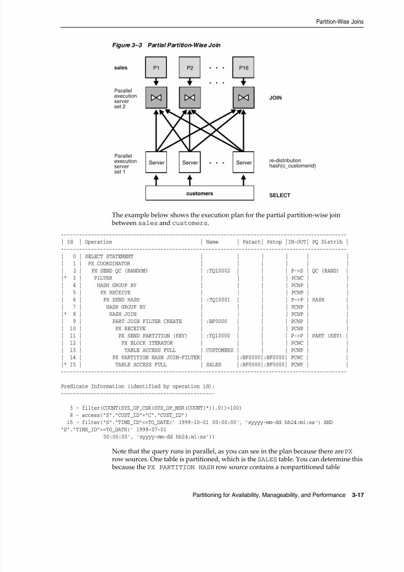
8/16/2019 Oracle Database VLDB and Partitioning Guide
http://slidepdf.com/reader/full/oracle-database-vldb-and-partitioning-guide 55/304
Partition-Wise Joins
Partitioning for Availability, Manageability, and Performance 3-17
Figure 3–3 Partial Partition-Wise Join
The example below shows the execution plan for the partial partition-wise join between sales and customers.
-----------------------------------------------------------------------------------------------| Id | Operation | Name | Pstart| Pstop |IN-OUT| PQ Distrib |-----------------------------------------------------------------------------------------------| 0 | SELECT STATEMENT | | | | | || 1 | PX COORDINATOR | | | | | || 2 | PX SEND QC (RANDOM) | :TQ10002 | | | P->S | QC (RAND) ||* 3 | FILTER | | | | PCWC | || 4 | HASH GROUP BY | | | | PCWP | || 5 | PX RECEIVE | | | | PCWP | |
| 6 | PX SEND HASH | :TQ10001 | | | P->P | HASH || 7 | HASH GROUP BY | | | | PCWP | ||* 8 | HASH JOIN | | | | PCWP | || 9 | PART JOIN FILTER CREATE | :BF0000 | | | PCWP | || 10 | PX RECEIVE | | | | PCWP | || 11 | PX SEND PARTITION (KEY) | :TQ10000 | | | P->P | PART (KEY) || 12 | PX BLOCK ITERATOR | | | | PCWC | || 13 | TABLE ACCESS FULL | CUSTOMERS | | | PCWP | || 14 | PX PARTITION HASH JOIN-FILTER| |:BF0000|:BF0000| PCWC | ||* 15 | TABLE ACCESS FULL | SALES |:BF0000|:BF0000| PCWP | |-----------------------------------------------------------------------------------------------
Predicate Information (identified by operation id):---------------------------------------------------
3 - filter(COUNT(SYS_OP_CSR(SYS_OP_MSR(COUNT(*)),0))>100) 8 - access("S"."CUST_ID"="C"."CUST_ID") 15 - filter("S"."TIME_ID"<=TO_DATE(' 1999-10-01 00:00:00', 'syyyy-mm-dd hh24:mi:ss') AND"S"."TIME_ID">=TO_DATE(' 1999-07-01 00:00:00', 'syyyy-mm-dd hh24:mi:ss'))
Note that the query runs in parallel, as you can see in the plan because there are PX row sources. One table is partitioned, which is the SALES table. You can determine this because the PX PARTITION HASH row source contains a nonpartitioned table
Server
P1
Server
P2
Server
P16
. . .
. . .
. . .
sales
Parallelexecutionserverset 2
Parallelexecutionserverset 1
customers
re-distributionhash(c_customerid)
JOIN
SELECT
8/16/2019 Oracle Database VLDB and Partitioning Guide
http://slidepdf.com/reader/full/oracle-database-vldb-and-partitioning-guide 56/304
Partition-Wise Joins
3-18 Oracle Database VLDB and Partitioning Guide
CUSTOMERS that is distributed through PX SEND PARTITION to a different slave setthat performs the join.
Considerations for full partition-wise joins also apply to partial partition-wise joins:
■ The degree of parallelism does not need to equal the number of partitions. InFigure 3–3, the query executes with two sets of 16 query servers. In this case,Oracle assigns 1 partition to each query server of the second set. Again, thenumber of partitions should always be a multiple of the degree of parallelism.
■ In Oracle Real Application Clusters environments on shared-nothing platforms(MPPs), each hash partition of sales should preferably have affinity to only one
node to avoid remote I/Os. Also, spread partitions over all nodes to avoid bottlenecks and use all CPU resources available on the system. A node can hostmultiple partitions when there are more partitions than nodes.
Partial Partition-Wise Joins: Composite
As with full partition-wise joins, the prime partitioning method for the sales table isto use the range method on column time_id. This is because sales is a typicalexample of a table that stores historical data. To enable a partial partition-wise joinwhile preserving this range partitioning, subpartition sales by hash on column
cust_id using 16 subpartitions for each partition. Both pruning and partialpartition-wise joins can be used if a query joins customers and sales and if thequery has a selection predicate on time_id.
When the sales table is composite partitioned, the granule of parallelism for a partialpartition-wise join is a hash partition and not a subpartition. Refer to Figure 3–2 for anillustration of a hash partition in a composite table. Again, the number of hashpartitions should be a multiple of the degree of parallelism. Also, on an MPP system,ensure that each hash partition has affinity to a single node. In the previous example,the eight subpartitions composing a hash partition should have affinity to the samenode.
The following example shows the execution plan for the query between sales andcustomers with sales range partitioned by time_id and subpartitioned by hash oncust_id.
---------------------------------------------------------------------------------------------| Id | Operation | Name | Pstart| Pstop |IN-OUT| PQ Distrib |---------------------------------------------------------------------------------------------| 0 | SELECT STATEMENT | | | | | |
Note: The Rows, Cost (%CPU), Time, and TQ columns wereremoved from the plan table output in this example.
Note: This section is based on hash partitioning, but it also appliesfor range, list, and interval partial partition-wise joins.
See Also: Oracle Real Application Clusters Administration andDeployment Guide for more information about data affinity
Note: This section is based on range-hash, but it also applies for all
other combinations of composite partial partition-wise joins.
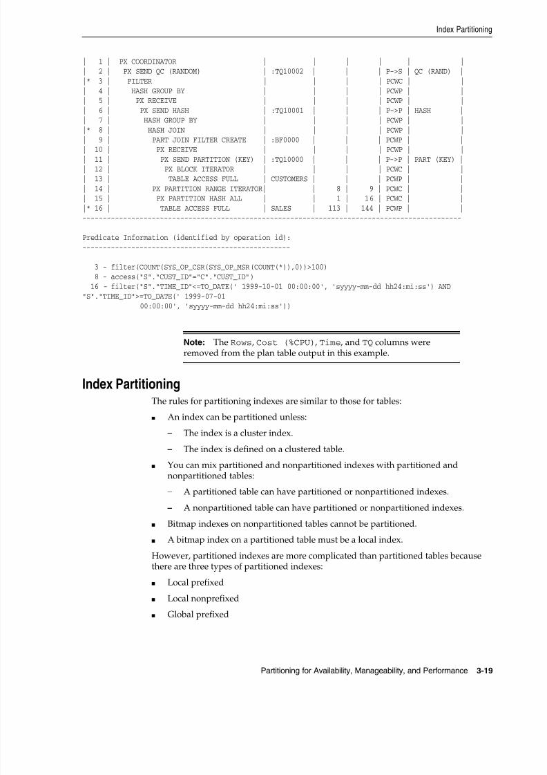
8/16/2019 Oracle Database VLDB and Partitioning Guide
http://slidepdf.com/reader/full/oracle-database-vldb-and-partitioning-guide 57/304
Index Partitioning
Partitioning for Availability, Manageability, and Performance 3-19
| 1 | PX COORDINATOR | | | | | || 2 | PX SEND QC (RANDOM) | :TQ10002 | | | P->S | QC (RAND) ||* 3 | FILTER | | | | PCWC | || 4 | HASH GROUP BY | | | | PCWP | || 5 | PX RECEIVE | | | | PCWP | || 6 | PX SEND HASH | :TQ10001 | | | P->P | HASH || 7 | HASH GROUP BY | | | | PCWP | ||* 8 | HASH JOIN | | | | PCWP | || 9 | PART JOIN FILTER CREATE | :BF0000 | | | PCWP | || 10 | PX RECEIVE | | | | PCWP | || 11 | PX SEND PARTITION (KEY) | :TQ10000 | | | P->P | PART (KEY) || 12 | PX BLOCK ITERATOR | | | | PCWC | || 13 | TABLE ACCESS FULL | CUSTOMERS | | | PCWP | || 14 | PX PARTITION RANGE ITERATOR| | 8 | 9 | PCWC | || 15 | PX PARTITION HASH ALL | | 1 | 16 | PCWC | ||* 16 | TABLE ACCESS FULL | SALES | 113 | 144 | PCWP | |---------------------------------------------------------------------------------------------
Predicate Information (identified by operation id):---------------------------------------------------
3 - filter(COUNT(SYS_OP_CSR(SYS_OP_MSR(COUNT(*)),0))>100) 8 - access("S"."CUST_ID"="C"."CUST_ID") 16 - filter("S"."TIME_ID"<=TO_DATE(' 1999-10-01 00:00:00', 'syyyy-mm-dd hh24:mi:ss') AND"S"."TIME_ID">=TO_DATE(' 1999-07-01 00:00:00', 'syyyy-mm-dd hh24:mi:ss'))
Index PartitioningThe rules for partitioning indexes are similar to those for tables:
■ An index can be partitioned unless:
– The index is a cluster index.
– The index is defined on a clustered table.
■ You can mix partitioned and nonpartitioned indexes with partitioned andnonpartitioned tables:
– A partitioned table can have partitioned or nonpartitioned indexes.
– A nonpartitioned table can have partitioned or nonpartitioned indexes.
■ Bitmap indexes on nonpartitioned tables cannot be partitioned.
■
A bitmap index on a partitioned table must be a local index.However, partitioned indexes are more complicated than partitioned tables becausethere are three types of partitioned indexes:
■ Local prefixed
■ Local nonprefixed
■ Global prefixed
Note: The Rows, Cost (%CPU), Time, and TQ columns wereremoved from the plan table output in this example.
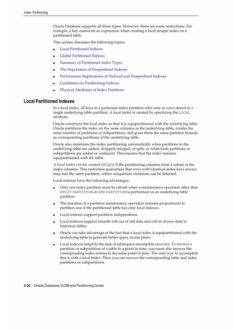
8/16/2019 Oracle Database VLDB and Partitioning Guide
http://slidepdf.com/reader/full/oracle-database-vldb-and-partitioning-guide 58/304
Index Partitioning
3-20 Oracle Database VLDB and Partitioning Guide
Oracle Database supports all three types. However, there are some restrictions. Forexample, a key cannot be an expression when creating a local unique index on apartitioned table.
This section discusses the following topics:
■ Local Partitioned Indexes
■
Global Partitioned Indexes■ Summary of Partitioned Index Types
■ The Importance of Nonprefixed Indexes
■ Performance Implications of Prefixed and Nonprefixed Indexes
■ Guidelines for Partitioning Indexes
■ Physical Attributes of Index Partitions
Local Partitioned IndexesIn a local index, all keys in a particular index partition refer only to rows stored in asingle underlying table partition. A local index is created by specifying the LOCAL
attribute.
Oracle constructs the local index so that it is equipartitioned with the underlying table.Oracle partitions the index on the same columns as the underlying table, creates thesame number of partitions or subpartitions, and gives them the same partition boundsas corresponding partitions of the underlying table.
Oracle also maintains the index partitioning automatically when partitions in theunderlying table are added, dropped, merged, or split, or when hash partitions orsubpartitions are added or coalesced. This ensures that the index remainsequipartitioned with the table.
A local index can be created UNIQUE if the partitioning columns form a subset of theindex columns. This restriction guarantees that rows with identical index keys always
map into the same partition, where uniqueness violations can be detected.
Local indexes have the following advantages:
■ Only one index partition must be rebuilt when a maintenance operation other thanSPLIT PARTITION or ADD PARTITION is performed on an underlying tablepartition.
■ The duration of a partition maintenance operation remains proportional topartition size if the partitioned table has only local indexes.
■ Local indexes support partition independence.
■ Local indexes support smooth roll-out of old data and roll-in of new data inhistorical tables.
■ Oracle can take advantage of the fact that a local index is equipartitioned with theunderlying table to generate better query access plans.
■ Local indexes simplify the task of tablespace incomplete recovery. To recover apartition or subpartition of a table to a point in time, you must also recover thecorresponding index entries to the same point in time. The only way to accomplishthis is with a local index. Then you can recover the corresponding table and indexpartitions or subpartitions.
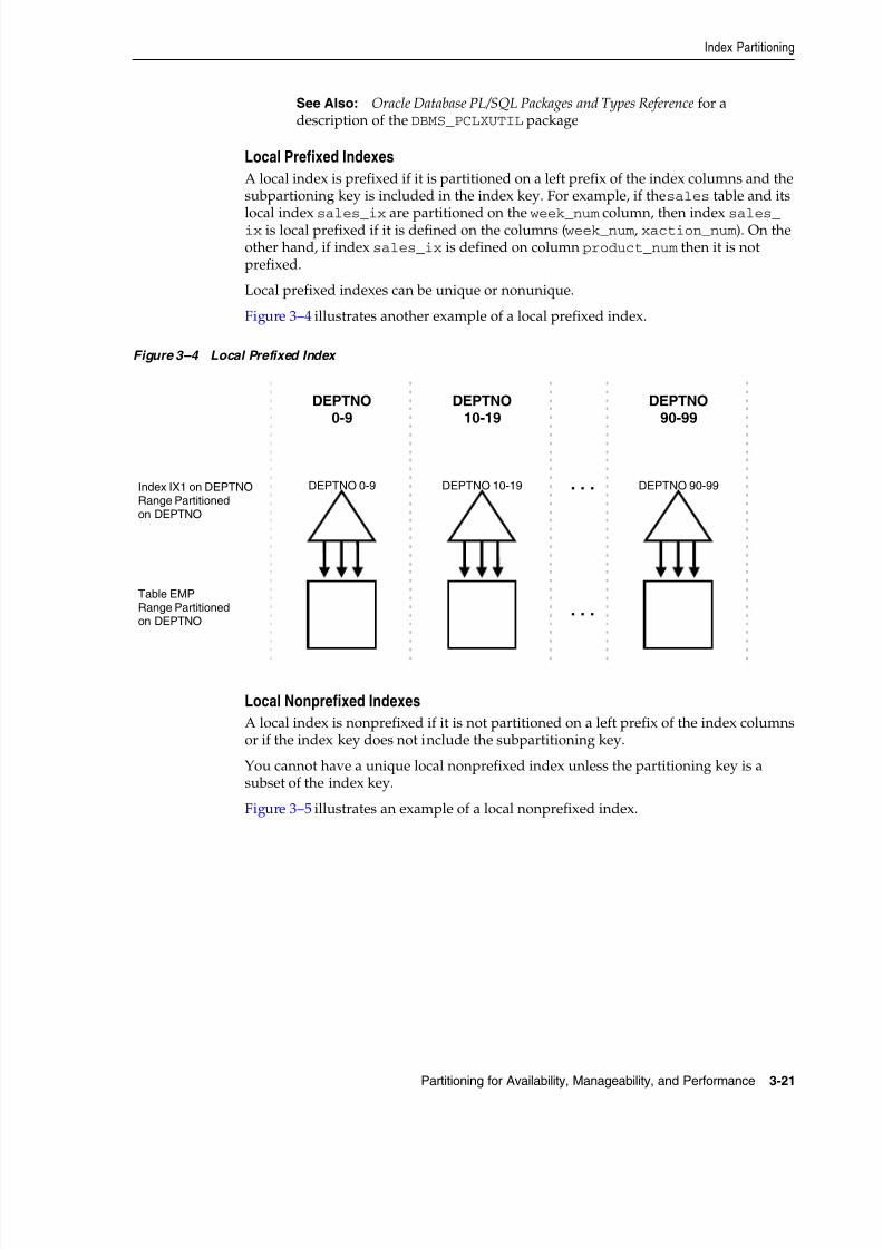
8/16/2019 Oracle Database VLDB and Partitioning Guide
http://slidepdf.com/reader/full/oracle-database-vldb-and-partitioning-guide 59/304
Index Partitioning
Partitioning for Availability, Manageability, and Performance 3-21
Local Prefixed Indexes
A local index is prefixed if it is partitioned on a left prefix of the index columns and thesubpartioning key is included in the index key. For example, if the sales table and its
local index sales_ix are partitioned on the week_num column, then index sales_ix is local prefixed if it is defined on the columns ( week_num , xaction_num ). On theother hand, if index sales_ix is defined on column product_num then it is notprefixed.
Local prefixed indexes can be unique or nonunique.
Figure 3–4 illustrates another example of a local prefixed index.
Figure 3–4 Local Prefixed Index
Local Nonprefixed Indexes
A local index is nonprefixed if it is not partitioned on a left prefix of the index columnsor if the index key does not include the subpartitioning key.
You cannot have a unique local nonprefixed index unless the partitioning key is asubset of the index key.
Figure 3–5 illustrates an example of a local nonprefixed index.
See Also: Oracle Database PL/SQL Packages and Types Reference for adescription of the DBMS_PCLXUTIL package
DEPTNO 0-9Index IX1 on DEPTNORange Partitionedon DEPTNO
Table EMPRange Partitionedon DEPTNO
DEPTNO0-9
DEPTNO 10-19
DEPTNO10-19
DEPTNO 90-99. . .
. . .
DEPTNO90-99
8/16/2019 Oracle Database VLDB and Partitioning Guide
http://slidepdf.com/reader/full/oracle-database-vldb-and-partitioning-guide 60/304
Index Partitioning
3-22 Oracle Database VLDB and Partitioning Guide
Figure 3–5 Local Nonprefixed Index
Global Partitioned IndexesIn a global partitioned index, the keys in a particular index partition may refer to rowsstored in multiple underlying table partitions or subpartitions. A global index can berange or hash partitioned, though it can be defined on any type of partitioned table.
A global index is created by specifying the GLOBAL attribute. The databaseadministrator is responsible for defining the initial partitioning of a global index atcreation and for maintaining the partitioning over time. Index partitions can bemerged or split as necessary.
Normally, a global index is not equipartitioned with the underlying table. There isnothing to prevent an index from being equipartitioned with the underlying table, butOracle does not take advantage of the equipartitioning when generating query plans
or executing partition maintenance operations. So an index that is equipartitioned withthe underlying table should be created as LOCAL.
A global partitioned index contains a single B-tree with entries for all rows in allpartitions. Each index partition may contain keys that refer to many differentpartitions or subpartitions in the table.
The highest partition of a global index must have a partition bound all of whose valuesare MAXVALUE. This insures that all rows in the underlying table can be represented inthe index.
Prefixed and Nonprefixed Global Partitioned Indexes
A global partitioned index is prefixed if it is partitioned on a left prefix of the index
columns. See Figure 3–6 for an example. A global partitioned index is nonprefixed if itis not partitioned on a left prefix of the index columns. Oracle does not support globalnonprefixed partitioned indexes.
Global prefixed partitioned indexes can be unique or nonunique.
Nonpartitioned indexes are treated as global prefixed nonpartitioned indexes.
Management of Global Partitioned Indexes
Global partitioned indexes are harder to manage than local indexes:
ACCTNO 31ACCTNO 82Index IX3 on ACCTNORange Partitionedon CHKDATE
Table CHECKSRange Partitionedon CHKDATE
CHKDATE
1/97
ACCTNO 54ACCTNO 82
CHKDATE
2/97
ACCTNO 15ACCTNO 35. . .
. . .
CHKDATE
12/97

8/16/2019 Oracle Database VLDB and Partitioning Guide
http://slidepdf.com/reader/full/oracle-database-vldb-and-partitioning-guide 61/304
Index Partitioning
Partitioning for Availability, Manageability, and Performance 3-23
■ When the data in an underlying table partition is moved or removed (SPLIT,MOVE, DROP, or TRUNCATE), all partitions of a global index are affected.Consequently global indexes do not support partition independence.
■ When an underlying table partition or subpartition is recovered to a point in time,all corresponding entries in a global index must be recovered to the same point intime. Because these entries may be scattered across all partitions or subpartitions
of the index, mixed in with entries for other partitions or subpartitions that are not being recovered, there is no way to accomplish this except by re-creating the entireglobal index.
Figure 3–6 Global Prefixed Partitioned Index
Summary of Partitioned Index TypesTable 3–1 summarizes the types of partitioned indexes that Oracle supports. The keypoints are:
■ If an index is local, it is equipartitioned with the underlying table. Otherwise, it isglobal.
■ A prefixed index is partitioned on a left prefix of the index columns. Otherwise, itis nonprefixed.
Table 3–1 Types of Partitioned Indexes
Type of Index
IndexEquipartitionedwith Table
IndexPartitioned onLeft Prefix ofIndex Columns
UNIQUEAttributeAllowed
Example:TablePartitioningKey
Example:IndexColumns
Example:IndexPartitioningKey
Local Prefixed (any
partitioning method)
Yes Yes Yes A A, B A
Local Nonprefixed(any partitioningmethod)
Yes No Yes1
1 For a unique local nonprefixed index, the partitioning key must be a subset of the index key.
A B, A A
Global Prefixed(range partitioningonly)
No2
2 Although a global partitioned index may be equipartitioned with the underlying table, Oracle does not take advantage of thepartitioning or maintain equipartitioning after partition maintenance operations such as DROP or SPLIT PARTITION.
Yes Yes A B B
EMPNO 15EMPNO 31Index IX3 on EMPNO
Range Partitionedon EMPNO
Table EMPRange Partitionedon DEPTNO
EMPNO0-39
EMPNO 54
EMPNO40-69
EMPNO 73EMPNO 82EMPNO 96. . .
. . .
EMPNO70-MAXVALUE
DEPTNO0-9
DEPTNO10-19
DEPTNO90-99

8/16/2019 Oracle Database VLDB and Partitioning Guide
http://slidepdf.com/reader/full/oracle-database-vldb-and-partitioning-guide 62/304
Index Partitioning
3-24 Oracle Database VLDB and Partitioning Guide
The Importance of Nonprefixed IndexesNonprefixed indexes are particularly useful in historical databases. In a tablecontaining historical data, it is common for an index to be defined on one column tosupport the requirements of fast access by that column, but partitioned on anothercolumn (the same column as the underlying table) to support the time interval forrolling out old data and rolling in new data.
Consider a sales table partitioned by week. It contains a year's worth of data,divided into 13 partitions. It is range partitioned on week_no, four weeks to apartition. You might create a nonprefixed local index sales_ix on sales. Thesales_ix index is defined on acct_no because there are queries that need fastaccess to the data by account number. However, it is partitioned on week_no to matchthe sales table. Every four weeks, the oldest partitions of sales and sales_ix aredropped and new ones are added.
Performance Implications of Prefixed and Nonprefixed IndexesIt is more expensive to probe into a nonprefixed index than to probe into a prefixedindex.
If an index is prefixed (either local or global) and Oracle is presented with a predicateinvolving the index columns, then partition pruning can restrict application of thepredicate to a subset of the index partitions.
For example, in Figure 3–4 on page 3-21, if the predicate is deptno=15, the optimizerknows to apply the predicate only to the second partition of the index. (If the predicateinvolves a bind variable, the optimizer does not know exactly which partition but itmay still know there is only one partition involved, in which case at run time, only oneindex partition is accessed.)
When an index is nonprefixed, Oracle often has to apply a predicate involving theindex columns to all N index partitions. This is required to look up a single key, or todo an index range scan. For a range scan, Oracle must also combine information fromN index partitions. For example, in Figure 3–5 on page 3-22, a local index is partitioned
on chkdate with an index key on acctno. If the predicate is acctno=31, Oracleprobes all 12 index partitions.
Of course, if there is also a predicate on the partitioning columns, then multiple indexprobes might not be necessary. Oracle takes advantage of the fact that a local index isequipartitioned with the underlying table to prune partitions based on the partitionkey. For example, if the predicate in Figure 3–4 on page 3-21 is chkdate<3/97, Oracleonly has to probe two partitions.
So for a nonprefixed index, if the partition key is a part of the WHERE clause but not ofthe index key, then the optimizer determines which index partitions to probe based onthe underlying table partition.
When many queries and DML statements using keys of local, nonprefixed, indexes
have to probe all index partitions, this effectively reduces the degree of partitionindependence provided by such indexes.
Table 3–2 Comparing Prefixed Local, Nonprefixed Local, and Global Indexes
IndexCharacteristics Prefixed Local
NonprefixedLocal Global
Unique possible? Yes Yes Yes. Must be global if using indexeson columns other than thepartitioning columns
8/16/2019 Oracle Database VLDB and Partitioning Guide
http://slidepdf.com/reader/full/oracle-database-vldb-and-partitioning-guide 63/304
Index Partitioning
Partitioning for Availability, Manageability, and Performance 3-25
Guidelines for Partitioning IndexesWhen deciding how to partition indexes on a table, consider the mix of applicationsthat must access the table. There is a trade-off between performance on the one handand availability and manageability on the other. Here are some guidelines you shouldconsider:
■ For OLTP applications:
– Global indexes and local prefixed indexes provide better performance thanlocal nonprefixed indexes because they minimize the number of index
partition probes.– Local indexes support more availability when there are partition or
subpartition maintenance operations on the table. Local nonprefixed indexesare very useful for historical databases.
■ For DSS applications, local nonprefixed indexes can improve performance becausemany index partitions can be scanned in parallel by range queries on the indexkey.
For example, a query using the predicate "acctno between 40 and 45" on the tablechecks of Figure 3–4 on page 3-21 causes parallel scans of all the partitions of thenonprefixed index ix3. On the other hand, a query using the predicate deptnoBETWEEN 40 AND 45 on the table deptno of Figure 3–5 on page 3-22 cannot beparallelized because it accesses a single partition of the prefixed index ix1.
■ For historical tables, indexes should be local if possible. This limits the impact ofregularly scheduled drop partition operations.
■ Unique indexes on columns other than the partitioning columns must be global because unique local nonprefixed indexes whose key does not contain thepartitioning key are not supported.
■ Unusable indexes do not consume space. See Oracle Database Administrator's Guide for more information.
Physical Attributes of Index PartitionsDefault physical attributes are initially specified when a CREATE INDEX statement
creates a partitioned index. Because there is no segment corresponding to thepartitioned index itself, these attributes are only used in derivation of physicalattributes of member partitions. Default physical attributes can later be modified usingALTER INDEX MODIFY DEFAULT ATTRIBUTES.
Physical attributes of partitions created by CREATE INDEX are determined as follows:
■ Values of physical attributes specified (explicitly or by default) for the index areused whenever the value of a corresponding partition attribute is not specified.Handling of the TABLESPACE attribute of partitions of a LOCAL index constitutesan important exception to this rule in that without a user-specified TABLESPACE
Manageability Easy to manage Easy to manage Harder to manage
OLTP Good Bad Good
Long Running(DSS)
Good Good Not Good
Table 3–2 (Cont.) Comparing Prefixed Local, Nonprefixed Local, and Global Indexes
IndexCharacteristics Prefixed Local
NonprefixedLocal Global

8/16/2019 Oracle Database VLDB and Partitioning Guide
http://slidepdf.com/reader/full/oracle-database-vldb-and-partitioning-guide 64/304

8/16/2019 Oracle Database VLDB and Partitioning Guide
http://slidepdf.com/reader/full/oracle-database-vldb-and-partitioning-guide 65/304
Partitioning and Table Compression
Partitioning for Availability, Manageability, and Performance 3-27
Table Compression and Bitmap IndexesTo use table compression on partitioned tables with bitmap indexes, you must do thefollowing before you introduce the compression attribute for the first time:
1. Mark bitmap indexes unusable.
2. Set the compression attribute.
3. Rebuild the indexes.
The first time you make a compressed partition part of an existing, fully
uncompressed partitioned table, you must either drop all existing bitmap indexes ormark them UNUSABLE before adding a compressed partition. This must be doneirrespective of whether any partition contains any data. It is also independent of theoperation that causes one or more compressed partitions to become part of the table.This does not apply to a partitioned table having B-tree indexes only.
This rebuilding of the bitmap index structures is necessary to accommodate thepotentially higher number of rows stored for each data block with table compressionenabled and must be done only for the first time. All subsequent operations, whetherthey affect compressed or uncompressed partitions, or change the compressionattribute, behave identically for uncompressed, partially compressed, or fullycompressed partitioned tables.
To avoid the recreation of any bitmap index structure, Oracle recommends creating
every partitioned table with at least one compressed partition whenever you plan topartially or fully compress the partitioned table in the future. This compressedpartition can stay empty or even can be dropped after the partition table creation.
Having a partitioned table with compressed partitions can lead to slightly larger bitmap index structures for the uncompressed partitions. The bitmap index structuresfor the compressed partitions, however, are usually smaller than the appropriate bitmap index structure before table compression. This highly depends on the achievedcompression rates.
Example of Table Compression and PartitioningThe following statement moves and compresses an existing partition sales_q1_1998 of table sales:
ALTER TABLE sales MOVE PARTITION sales_q1_1998 TABLESPACE ts_arch_q1_1998 COMPRESS;
See Also:
■ Oracle Database Data Warehousing Guide for a generic discussion oftable compression
■ Oracle Database Administrator's Guide for more detailedinformation
■ Oracle Database Performance Tuning Guide for an example ofcalculating the compression ratio
Note: Oracle Database raises an error if compression is introduced toan object for the first time and there are usable bitmap indexsegments.

8/16/2019 Oracle Database VLDB and Partitioning Guide
http://slidepdf.com/reader/full/oracle-database-vldb-and-partitioning-guide 66/304
Recommendations for Choosing a Partitioning Strategy
3-28 Oracle Database VLDB and Partitioning Guide
If you use the MOVE statement, the local indexes for partition sales_q1_1998 becomeunusable. You must rebuild them afterward, as follows:
ALTER TABLE sales MODIFY PARTITION sales_q1_1998 REBUILD UNUSABLE LOCAL INDEXES;
You can also include the UPDATE INDEXES clause in the MOVE statement in order forthe entire operation to be completed automatically without any negative impact onusers accessing the table.
The following statement merges two existing partitions into a new, compressedpartition, residing in a separate tablespace. The local bitmap indexes have to be rebuiltafterward, as in the following:
ALTER TABLE sales MERGE PARTITIONS sales_q1_1998, sales_q2_1998INTO PARTITION sales_1_1998 TABLESPACE ts_arch_1_1998COMPRESS FOR OLTP UPDATE INDEXES;
For more details and examples for partition management operations, refer toChapter 4, "Partition Administration".
Recommendations for Choosing a Partitioning StrategyThe following sections provide recommendations for choosing a partitioning strategy:
■ When to Use Range or Interval Partitioning
■ When to Use Hash Partitioning
■ When to Use List Partitioning
■ When to Use Composite Partitioning
■ When to Use Interval Partitioning
■ When to Use Reference Partitioning
■ When to Partition on Virtual Columns
■ Considerations When Using Read-Only Tablespaces
When to Use Range or Interval PartitioningRange partitioning is a convenient method for partitioning historical data. The boundaries of range partitions define the ordering of the partitions in the tables or
indexes.Interval partitioning is an extension to range partitioning in which, beyond a point intime, partitions are defined by an interval. Interval partitions are automatically created by the database when data is inserted into the partition.
Range or interval partitioning is often used to organize data by time intervals on acolumn of type DATE. Thus, most SQL statements accessing range partitions focus ontimeframes. An example of this is a SQL statement similar to "select data from aparticular period in time." In such a scenario, if each partition represents data for onemonth, the query "find data of month 06-DEC" must access only the December
See Also:
■ Oracle Database Performance Tuning Guide for details regarding howto estimate the compression ratio when using table compression
■ Oracle Database SQL Language Reference for the SQL syntax

8/16/2019 Oracle Database VLDB and Partitioning Guide
http://slidepdf.com/reader/full/oracle-database-vldb-and-partitioning-guide 67/304
Recommendations for Choosing a Partitioning Strategy
Partitioning for Availability, Manageability, and Performance 3-29
partition of year 2006. This reduces the amount of data scanned to a fraction of thetotal data available, an optimization method called partition pruning.
Range partitioning is also ideal when you periodically load new data and purge olddata, because it is easy to add or drop partitions.
It is common to keep a rolling window of data, for example keeping the past 36months' worth of data online. Range partitioning simplifies this process. To add data
from a new month, you load it into a separate table, clean it, index it, and then add itto the range-partitioned table using the EXCHANGE PARTITION statement, all whilethe original table remains online. After you add the new partition, you can drop thetrailing month with the DROP PARTITION statement. The alternative to using theDROP PARTITION statement can be to archive the partition and make it read only, butthis works only when your partitions are in separate tablespaces. You can alsoimplement a rolling window data using inserts into the partitioned table.
Interval partitioning provides an easy way for interval partitions to be automaticallycreated as data arrives. Interval partitions can also be used for all other partitionmaintenance operations. Refer to Chapter 4, "Partition Administration" for moreinformation about the partition maintenance operations on interval partitions.
In conclusion, consider using range or interval partitioning when:
■ Very large tables are frequently scanned by a range predicate on a goodpartitioning column, such as ORDER_DATE or PURCHASE_DATE. Partitioning thetable on that column enables partition pruning.
■ You want to maintain a rolling window of data.
■ You cannot complete administrative operations, such as backup and restore, onlarge tables in an allotted time frame, but you can divide them into smaller logicalpieces based on the partition range column.
The following example creates the table salestable for a period of two years, 2005and 2006, and partitions it by range according to the column s_salesdate toseparate the data into eight quarters, each corresponding to a partition. Future
partitions are created automatically through the monthly interval definition. Intervalpartitions are created in the provided list of tablespaces in a round-robin manner.Analysis of sales figures by a short interval can take advantage of partition pruning.The sales table also supports a rolling window approach.
Example 3–3 Creating a table with range and interval partitioning
CREATE TABLE salestable (s_productid NUMBER, s_saledate DATE, s_custid NUMBER, s_totalprice NUMBER)PARTITION BY RANGE(s_saledate)INTERVAL(NUMTOYMINTERVAL(1,'MONTH')) STORE IN (tbs1,tbs2,tbs3,tbs4)
(PARTITION sal05q1 VALUES LESS THAN (TO_DATE('01-APR-2005', 'DD-MON-YYYY')) TABLESPACE tbs1, PARTITION sal05q2 VALUES LESS THAN (TO_DATE('01-JUL-2005', 'DD-MON-YYYY'))
TABLESPACE tbs2, PARTITION sal05q3 VALUES LESS THAN (TO_DATE('01-OCT-2005', 'DD-MON-YYYY'))
TABLESPACE tbs3, PARTITION sal05q4 VALUES LESS THAN (TO_DATE('01-JAN-2006', 'DD-MON-YYYY'))
TABLESPACE tbs4, PARTITION sal06q1 VALUES LESS THAN (TO_DATE('01-APR-2006', 'DD-MON-YYYY'))
TABLESPACE tbs1, PARTITION sal06q2 VALUES LESS THAN (TO_DATE('01-JUL-2006', 'DD-MON-YYYY'))

8/16/2019 Oracle Database VLDB and Partitioning Guide
http://slidepdf.com/reader/full/oracle-database-vldb-and-partitioning-guide 68/304
Recommendations for Choosing a Partitioning Strategy
3-30 Oracle Database VLDB and Partitioning Guide
TABLESPACE tbs2, PARTITION sal06q3 VALUES LESS THAN (TO_DATE('01-OCT-2006', 'DD-MON-YYYY'))
TABLESPACE tbs3, PARTITION sal06q4 VALUES LESS THAN (TO_DATE('01-JAN-2007', 'DD-MON-YYYY'))
TABLESPACE tbs4);
When to Use Hash PartitioningThere are times when it is not obvious into which partition data should reside,although the partitioning key can be identified. Rather than group similar data, thereare times when it is desirable to distribute data such that it does not correspond to a business or a logical view of the data, as it does in range partitioning. With hashpartitioning, a row is placed into a partition based on the result of passing thepartitioning key into a hashing algorithm.
Using this approach, data is randomly distributed across the partitions rather thangrouped. This is a good approach for some data, but may not be an effective way tomanage historical data. However, hash partitions share some performancecharacteristics with range partitions. For example, partition pruning is limited toequality predicates. You can also use partition-wise joins, parallel index access, andparallel DML. See "Partition-Wise Joins" on page 3-11 for more information.
As a general rule, use hash partitioning for the following purposes:
■ To enable partial or full parallel partition-wise joins with very likely equisizedpartitions.
■ To distribute data evenly among the nodes of an MPP platform that uses OracleReal Application Clusters. Consequently, you can minimize interconnect trafficwhen processing internode parallel statements.
■ To use partition pruning and partition-wise joins according to a partitioning keythat is mostly constrained by a distinct value or value list.
■ To randomly distribute data to avoid I/O bottlenecks if you do not use a storagemanagement technique that stripes and mirrors across all available devices.
For more information, refer to Chapter 10, "Storage Management for VLDBs".
For optimal data distribution, the following requirements should be satisfied:
■ Choose a column or combination of columns that is unique or almost unique.
■ Create multiple partitions and subpartitions for each partition that is a power oftwo. For example, 2, 4, 8, 16, 32, 64, 128, and so on.
The following example creates four hash partitions for the table sales_hash usingthe column s_productid as the partitioning key. Parallel joins with the productstable can take advantage of partial or full partition-wise joins. Queries accessing salesfigures for only a single product or a list of products benefit from partition pruning.
Example 3–4 Creating a table with hash partitioning
CREATE TABLE sales_hash (s_productid NUMBER, s_saledate DATE, s_custid NUMBER,
Note: With hash partitioning, only equality or IN-list predicates aresupported for partition pruning.
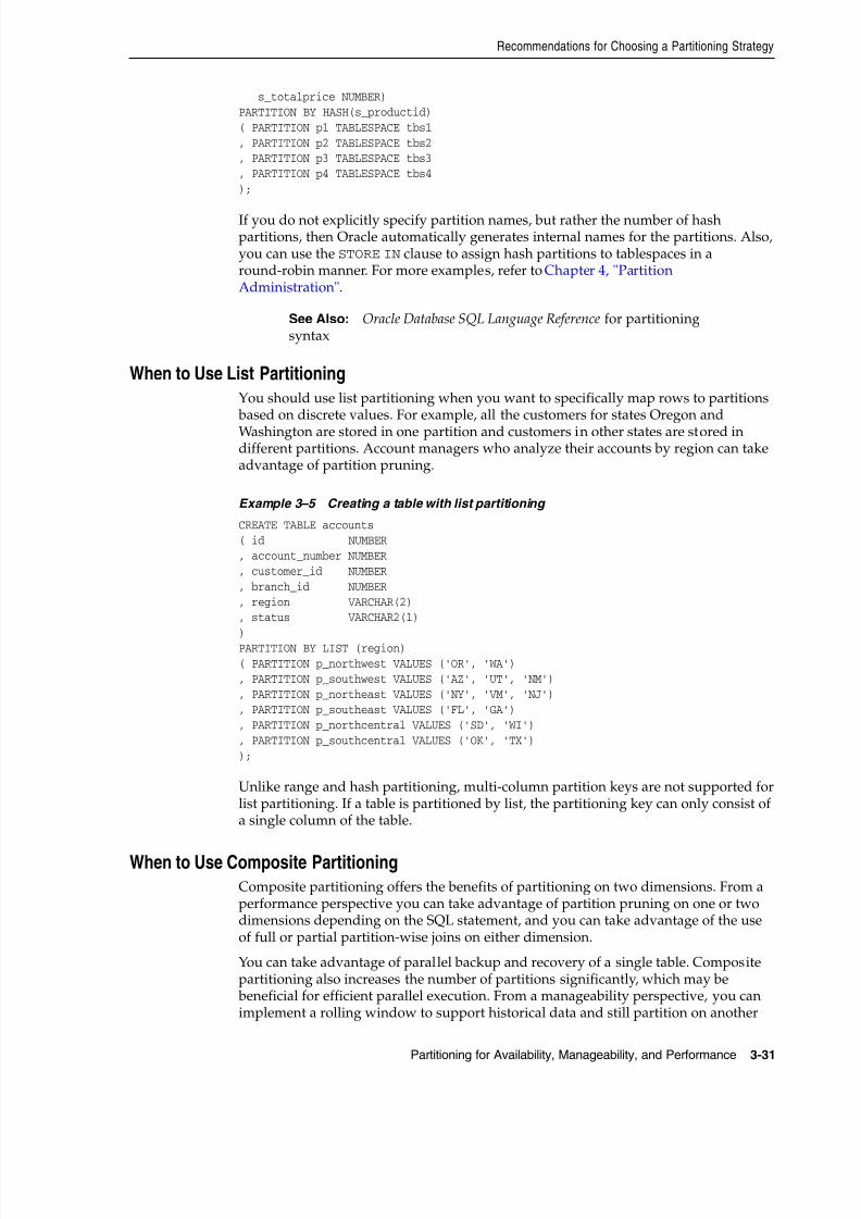
8/16/2019 Oracle Database VLDB and Partitioning Guide
http://slidepdf.com/reader/full/oracle-database-vldb-and-partitioning-guide 69/304
Recommendations for Choosing a Partitioning Strategy
Partitioning for Availability, Manageability, and Performance 3-31
s_totalprice NUMBER)PARTITION BY HASH(s_productid)( PARTITION p1 TABLESPACE tbs1, PARTITION p2 TABLESPACE tbs2, PARTITION p3 TABLESPACE tbs3, PARTITION p4 TABLESPACE tbs4);
If you do not explicitly specify partition names, but rather the number of hashpartitions, then Oracle automatically generates internal names for the partitions. Also,you can use the STORE IN clause to assign hash partitions to tablespaces in around-robin manner. For more examples, refer to Chapter 4, "PartitionAdministration".
When to Use List PartitioningYou should use list partitioning when you want to specifically map rows to partitions based on discrete values. For example, all the customers for states Oregon and
Washington are stored in one partition and customers in other states are stored indifferent partitions. Account managers who analyze their accounts by region can takeadvantage of partition pruning.
Example 3–5 Creating a table with list partitioning
CREATE TABLE accounts( id NUMBER, account_number NUMBER, customer_id NUMBER, branch_id NUMBER, region VARCHAR(2), status VARCHAR2(1))PARTITION BY LIST (region)( PARTITION p_northwest VALUES ('OR', 'WA'), PARTITION p_southwest VALUES ('AZ', 'UT', 'NM'), PARTITION p_northeast VALUES ('NY', 'VM', 'NJ'), PARTITION p_southeast VALUES ('FL', 'GA'), PARTITION p_northcentral VALUES ('SD', 'WI'), PARTITION p_southcentral VALUES ('OK', 'TX'));
Unlike range and hash partitioning, multi-column partition keys are not supported forlist partitioning. If a table is partitioned by list, the partitioning key can only consist ofa single column of the table.
When to Use Composite PartitioningComposite partitioning offers the benefits of partitioning on two dimensions. From aperformance perspective you can take advantage of partition pruning on one or twodimensions depending on the SQL statement, and you can take advantage of the useof full or partial partition-wise joins on either dimension.
You can take advantage of parallel backup and recovery of a single table. Compositepartitioning also increases the number of partitions significantly, which may be beneficial for efficient parallel execution. From a manageability perspective, you canimplement a rolling window to support historical data and still partition on another
See Also: Oracle Database SQL Language Reference for partitioningsyntax
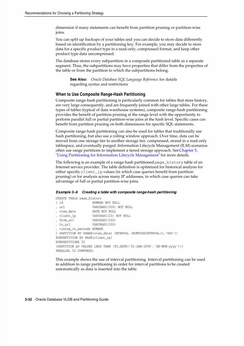
8/16/2019 Oracle Database VLDB and Partitioning Guide
http://slidepdf.com/reader/full/oracle-database-vldb-and-partitioning-guide 70/304
Recommendations for Choosing a Partitioning Strategy
3-32 Oracle Database VLDB and Partitioning Guide
dimension if many statements can benefit from partition pruning or partition-wise joins.
You can split up backups of your tables and you can decide to store data differently based on identification by a partitioning key. For example, you may decide to storedata for a specific product type in a read-only, compressed format, and keep otherproduct type data uncompressed.
The database stores every subpartition in a composite partitioned table as a separatesegment. Thus, the subpartitions may have properties that differ from the properties ofthe table or from the partition to which the subpartitions belong.
When to Use Composite Range-Hash Partitioning
Composite range-hash partitioning is particularly common for tables that store history,are very large consequently, and are frequently joined with other large tables. For thesetypes of tables (typical of data warehouse systems), composite range-hash partitioningprovides the benefit of partition pruning at the range level with the opportunity to
perform parallel full or partial partition-wise joins at the hash level. Specific cases can benefit from partition pruning on both dimensions for specific SQL statements.
Composite range-hash partitioning can also be used for tables that traditionally usehash partitioning, but also use a rolling window approach. Over time, data can bemoved from one storage tier to another storage tier, compressed, stored in a read-onlytablespace, and eventually purged. Information Lifecycle Management (ILM) scenariosoften use range partitions to implement a tiered storage approach. See Chapter 5,"Using Partitioning for Information Lifecycle Management" for more details.
The following is an example of a range-hash partitioned page_history table of anInternet service provider. The table definition is optimized for historical analysis foreither specific client_ip values (in which case queries benefit from partitionpruning) or for analysis across many IP addresses, in which case queries can take
advantage of full or partial partition-wise joins.
Example 3–6 Creating a table with composite range-hash partitioning
CREATE TABLE page_history( id NUMBER NOT NULL, url VARCHAR2(300) NOT NULL, view_date DATE NOT NULL, client_ip VARCHAR2(23) NOT NULL, from_url VARCHAR2(300), to_url VARCHAR2(300), timing_in_seconds NUMBER) PARTITION BY RANGE(view_date) INTERVAL (NUMTODSINTERVAL(1,'DAY'))SUBPARTITION BY HASH(client_ip)
SUBPARTITIONS 32(PARTITION p0 VALUES LESS THAN (TO_DATE('01-JAN-2006','dd-MON-yyyy')))PARALLEL 32 COMPRESS;
This example shows the use of interval partitioning. Interval partitioning can be usedin addition to range partitioning in order for interval partitions to be createdautomatically as data is inserted into the table.
See Also: Oracle Database SQL Language Reference for detailsregarding syntax and restrictions
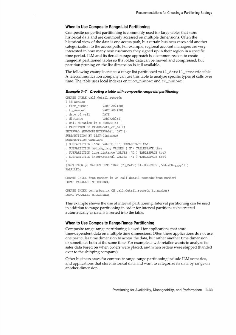
8/16/2019 Oracle Database VLDB and Partitioning Guide
http://slidepdf.com/reader/full/oracle-database-vldb-and-partitioning-guide 71/304
Recommendations for Choosing a Partitioning Strategy
Partitioning for Availability, Manageability, and Performance 3-33
When to Use Composite Range-List Partitioning
Composite range-list partitioning is commonly used for large tables that storehistorical data and are commonly accessed on multiple dimensions. Often thehistorical view of the data is one access path, but certain business cases add anothercategorization to the access path. For example, regional account managers are veryinterested in how many new customers they signed up in their region in a specifictime period. ILM and its tiered storage approach is a common reason to createrange-list partitioned tables so that older data can be moved and compressed, butpartition pruning on the list dimension is still available.
The following example creates a range-list partitioned call_detail_records table.A telecommunication company can use this table to analyze specific types of calls overtime. The table uses local indexes on from_number and to_number.
Example 3–7 Creating a table with composite range-list partitioning
CREATE TABLE call_detail_records( id NUMBER, from_number VARCHAR2(20), to_number VARCHAR2(20), date_of_call DATE
, distance VARCHAR2(1), call_duration_in_s NUMBER(4)) PARTITION BY RANGE(date_of_call)INTERVAL (NUMTODSINTERVAL(1,'DAY'))SUBPARTITION BY LIST(distance)SUBPARTITION TEMPLATE( SUBPARTITION local VALUES('L') TABLESPACE tbs1, SUBPARTITION medium_long VALUES ('M') TABLESPACE tbs2, SUBPARTITION long_distance VALUES ('D') TABLESPACE tbs3, SUBPARTITION international VALUES ('I') TABLESPACE tbs4)(PARTITION p0 VALUES LESS THAN (TO_DATE('01-JAN-2005','dd-MON-yyyy')))PARALLEL;
CREATE INDEX from_number_ix ON call_detail_records(from_number)LOCAL PARALLEL NOLOGGING;
CREATE INDEX to_number_ix ON call_detail_records(to_number)LOCAL PARALLEL NOLOGGING;
This example shows the use of interval partitioning. Interval partitioning can be usedin addition to range partitioning in order for interval partitions to be createdautomatically as data is inserted into the table.
When to Use Composite Range-Range Partitioning
Composite range-range partitioning is useful for applications that store
time-dependent data on multiple time dimensions. Often these applications do not useone particular time dimension to access the data, but rather another time dimension,or sometimes both at the same time. For example, a web retailer wants to analyze itssales data based on when orders were placed, and when orders were shipped (handedover to the shipping company).
Other business cases for composite range-range partitioning include ILM scenarios,and applications that store historical data and want to categorize its data by range onanother dimension.

8/16/2019 Oracle Database VLDB and Partitioning Guide
http://slidepdf.com/reader/full/oracle-database-vldb-and-partitioning-guide 72/304
Recommendations for Choosing a Partitioning Strategy
3-34 Oracle Database VLDB and Partitioning Guide
The following example shows a range-range partitioned table account_balance_history. A bank may use access to individual subpartitions to contact its customersfor low-balance reminders or specific promotions relevant to a certain category ofcustomers.
Example 3–8 Creating a table with composite range-range partitioning
CREATE TABLE account_balance_history( id NUMBER NOT NULL, account_number NUMBER NOT NULL, customer_id NUMBER NOT NULL, transaction_date DATE NOT NULL, amount_credited NUMBER, amount_debited NUMBER, end_of_day_balance NUMBER NOT NULL) PARTITION BY RANGE(transaction_date)INTERVAL (NUMTODSINTERVAL(7,'DAY'))SUBPARTITION BY RANGE(end_of_day_balance)SUBPARTITION TEMPLATE( SUBPARTITION unacceptable VALUES LESS THAN (-1000), SUBPARTITION credit VALUES LESS THAN (0)
, SUBPARTITION low VALUES LESS THAN (500), SUBPARTITION normal VALUES LESS THAN (5000), SUBPARTITION high VALUES LESS THAN (20000), SUBPARTITION extraordinary VALUES LESS THAN (MAXVALUE))(PARTITION p0 VALUES LESS THAN (TO_DATE('01-JAN-2007','dd-MON-yyyy')));
This example shows the use of interval partitioning. Interval partitioning can be usedin addition to range partitioning in order for interval partitions to be createdautomatically as data is inserted into the table. In this case 7-day (weekly) intervals arecreated, starting Monday, January 1, 2007.
When to Use Composite List-Hash Partitioning
Composite list-hash partitioning is useful for large tables that are usually accessed onone dimension, but (due to their size) still must take advantage of parallel full orpartial partition-wise joins on another dimension in joins with other large tables.
The following example shows a credit_card_accounts table. The table islist-partitioned on region in order for account managers to quickly access accounts intheir region. The subpartitioning strategy is hash on customer_id so that queriesagainst the transactions table, also subpartitioned on customer_id, can takeadvantage of full partition-wise joins. Joins with the hash-partitioned customers tablecan also benefit from full partition-wise joins. The table has a local bitmap index on theis_active column.
Example 3–9 Creating a table with composite list-hash partitioning
CREATE TABLE credit_card_accounts( account_number NUMBER(16) NOT NULL, customer_id NUMBER NOT NULL, customer_region VARCHAR2(2) NOT NULL, is_active VARCHAR2(1) NOT NULL, date_opened DATE NOT NULL) PARTITION BY LIST (customer_region)SUBPARTITION BY HASH (customer_id)SUBPARTITIONS 16( PARTITION emea VALUES ('EU','ME','AF'), PARTITION amer VALUES ('NA','LA')
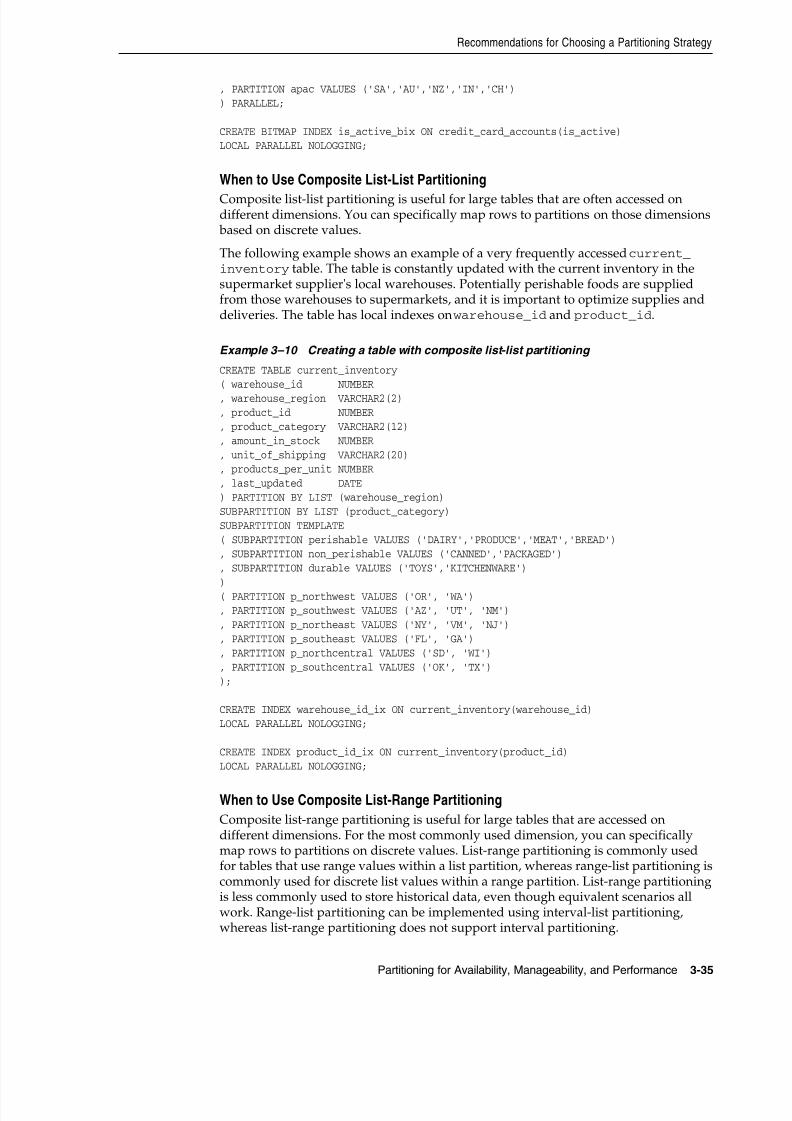
8/16/2019 Oracle Database VLDB and Partitioning Guide
http://slidepdf.com/reader/full/oracle-database-vldb-and-partitioning-guide 73/304
Recommendations for Choosing a Partitioning Strategy
Partitioning for Availability, Manageability, and Performance 3-35
, PARTITION apac VALUES ('SA','AU','NZ','IN','CH')) PARALLEL;
CREATE BITMAP INDEX is_active_bix ON credit_card_accounts(is_active)LOCAL PARALLEL NOLOGGING;
When to Use Composite List-List Partitioning
Composite list-list partitioning is useful for large tables that are often accessed ondifferent dimensions. You can specifically map rows to partitions on those dimensions based on discrete values.
The following example shows an example of a very frequently accessed current_inventory table. The table is constantly updated with the current inventory in thesupermarket supplier's local warehouses. Potentially perishable foods are suppliedfrom those warehouses to supermarkets, and it is important to optimize supplies anddeliveries. The table has local indexes on warehouse_id and product_id.
Example 3–10 Creating a table with composite list-list partitioning
CREATE TABLE current_inventory( warehouse_id NUMBER, warehouse_region VARCHAR2(2), product_id NUMBER, product_category VARCHAR2(12), amount_in_stock NUMBER, unit_of_shipping VARCHAR2(20), products_per_unit NUMBER, last_updated DATE) PARTITION BY LIST (warehouse_region)SUBPARTITION BY LIST (product_category)SUBPARTITION TEMPLATE( SUBPARTITION perishable VALUES ('DAIRY','PRODUCE','MEAT','BREAD'), SUBPARTITION non_perishable VALUES ('CANNED','PACKAGED'), SUBPARTITION durable VALUES ('TOYS','KITCHENWARE'))( PARTITION p_northwest VALUES ('OR', 'WA'), PARTITION p_southwest VALUES ('AZ', 'UT', 'NM'), PARTITION p_northeast VALUES ('NY', 'VM', 'NJ'), PARTITION p_southeast VALUES ('FL', 'GA'), PARTITION p_northcentral VALUES ('SD', 'WI'), PARTITION p_southcentral VALUES ('OK', 'TX'));
CREATE INDEX warehouse_id_ix ON current_inventory(warehouse_id)LOCAL PARALLEL NOLOGGING;
CREATE INDEX product_id_ix ON current_inventory(product_id)LOCAL PARALLEL NOLOGGING;
When to Use Composite List-Range Partitioning
Composite list-range partitioning is useful for large tables that are accessed ondifferent dimensions. For the most commonly used dimension, you can specificallymap rows to partitions on discrete values. List-range partitioning is commonly usedfor tables that use range values within a list partition, whereas range-list partitioning iscommonly used for discrete list values within a range partition. List-range partitioningis less commonly used to store historical data, even though equivalent scenarios allwork. Range-list partitioning can be implemented using interval-list partitioning,whereas list-range partitioning does not support interval partitioning.

8/16/2019 Oracle Database VLDB and Partitioning Guide
http://slidepdf.com/reader/full/oracle-database-vldb-and-partitioning-guide 74/304
Recommendations for Choosing a Partitioning Strategy
3-36 Oracle Database VLDB and Partitioning Guide
The following example shows a donations table that stores donations in differentcurrencies. The donations are categorized into small, medium, and high, depending onthe amount. Due to currency differences, the ranges are different.
Example 3–11 Creating a table with composite list-range partitioning
CREATE TABLE donations( id NUMBER, name VARCHAR2(60), beneficiary VARCHAR2(80), payment_method VARCHAR2(30), currency VARCHAR2(3), amount NUMBER) PARTITION BY LIST (currency)SUBPARTITION BY RANGE (amount)( PARTITION p_eur VALUES ('EUR') ( SUBPARTITION p_eur_small VALUES LESS THAN (8) , SUBPARTITION p_eur_medium VALUES LESS THAN (80) , SUBPARTITION p_eur_high VALUES LESS THAN (MAXVALUE) ), PARTITION p_gbp VALUES ('GBP')
( SUBPARTITION p_gbp_small VALUES LESS THAN (5) , SUBPARTITION p_gbp_medium VALUES LESS THAN (50) , SUBPARTITION p_gbp_high VALUES LESS THAN (MAXVALUE) ), PARTITION p_aud_nzd_chf VALUES ('AUD','NZD','CHF') ( SUBPARTITION p_aud_nzd_chf_small VALUES LESS THAN (12) , SUBPARTITION p_aud_nzd_chf_medium VALUES LESS THAN (120) , SUBPARTITION p_aud_nzd_chf_high VALUES LESS THAN (MAXVALUE) ), PARTITION p_jpy VALUES ('JPY') ( SUBPARTITION p_jpy_small VALUES LESS THAN (1200) , SUBPARTITION p_jpy_medium VALUES LESS THAN (12000) , SUBPARTITION p_jpy_high VALUES LESS THAN (MAXVALUE) )
, PARTITION p_inr VALUES ('INR') ( SUBPARTITION p_inr_small VALUES LESS THAN (400) , SUBPARTITION p_inr_medium VALUES LESS THAN (4000) , SUBPARTITION p_inr_high VALUES LESS THAN (MAXVALUE) ), PARTITION p_zar VALUES ('ZAR') ( SUBPARTITION p_zar_small VALUES LESS THAN (70) , SUBPARTITION p_zar_medium VALUES LESS THAN (700) , SUBPARTITION p_zar_high VALUES LESS THAN (MAXVALUE) ), PARTITION p_default VALUES (DEFAULT) ( SUBPARTITION p_default_small VALUES LESS THAN (10) , SUBPARTITION p_default_medium VALUES LESS THAN (100) , SUBPARTITION p_default_high VALUES LESS THAN (MAXVALUE)
)) ENABLE ROW MOVEMENT;
When to Use Interval PartitioningInterval partitioning can be used for every table that is range partitioned and usesfixed intervals for new partitions. The database automatically creates intervalpartitions as data for that partition arrives. Until this happens, the interval partitionexists but no segment is created for the partition.
8/16/2019 Oracle Database VLDB and Partitioning Guide
http://slidepdf.com/reader/full/oracle-database-vldb-and-partitioning-guide 75/304
Recommendations for Choosing a Partitioning Strategy
Partitioning for Availability, Manageability, and Performance 3-37
The benefit of interval partitioning is that you do not need to create your rangepartitions explicitly. You should consider using interval partitioning unless you createrange partitions with different intervals, or if you always set specific partitionattributes when you create range partitions. Note that you can specify a list oftablespaces in the interval definition. The database creates interval partitions in theprovided list of tablespaces in a round-robin manner.
If you upgrade your application and you use range partitioning or composite range-*partitioning, then you can easily change your existing table definition to use intervalpartitioning. Note that you cannot manually add partitions to an interval-partitionedtable. If you have automated the creation of new partitions, then you must changeyour application code to prevent the explicit creation of range partitions goingforward.
The following example shows how to change the sales table in the sample sh schema from range partitioning to start using monthly interval partitioning.
ALTER TABLE sales SET INTERVAL (NUMTOYMINTERVAL(1,'MONTH'));
You cannot use interval partitioning with reference partitioned tables.
Serializable transactions do not work with interval partitioning. Inserting data into a
partition of an interval partitioned table that does not have a segment yet causes anerror.
When to Use Reference PartitioningReference partitioning is useful in the following scenarios:
■ If you have denormalized, or would denormalize, a column from a master tableinto a child table to get partition pruning benefits on both tables.
For example, your orders table stores the order_date, but the order_items table, which stores one or more items per order, does not. To get good performancefor historical analysis of orders data, you would traditionally duplicate theorder_date column in the order_items table to get partition pruning on theorder_items table.
You should consider reference partitioning in such a scenario and avoid having toduplicate the order_date column. Queries that join both tables and use apredicate on order_date automatically benefit from partition pruning on bothtables.
■ If two large tables are joined frequently, then the tables are not partitioned on the join key, but you want to take advantage of partition-wise joins.
Reference partitioning implicitly enables full partition-wise joins.
■ If data in multiple tables has a related life cycle, then reference partitioning canprovide significant manageability benefits.
Partition management operations against the master table are automaticallycascaded to its descendents. For example, when you add a partition to the mastertable, that creation is automatically propagated to all its descendents.
To use reference partitioning, you must enable and enforce the foreign keyrelationship between the master table and the reference table in place. You cancascade reference-partitioned tables.

8/16/2019 Oracle Database VLDB and Partitioning Guide
http://slidepdf.com/reader/full/oracle-database-vldb-and-partitioning-guide 76/304
Recommendations for Choosing a Partitioning Strategy
3-38 Oracle Database VLDB and Partitioning Guide
When to Partition on Virtual ColumnsVirtual column partitioning enables you to partition on an expression, which may usedata from other columns, and perform calculations with these columns. PL/SQLfunction calls are not supported in virtual column definitions that are to be used as apartitioning key.
Virtual column partitioning supports all partitioning methods, plus performance and
manageability features. You should consider using virtual columns if tables arefrequently accessed using a predicate that is not directly captured in a column, but can be derived, to get partition pruning benefits. Traditionally, to get partition pruning benefits, you would have to add a separate column to capture and calculate the correctvalue and ensure the column is always populated correctly to ensure correct queryretrieval.
The following example shows a car_rentals table. The customer's confirmationnumber contains a two-character country name as the location where the rental car ispicked up. Rental car analyses usually evaluate regional patterns, so it makes sense topartition by country.
Example 3–12 Creating a table with virtual columns for partitioning
CREATE TABLE car_rentals( id NUMBER NOT NULL , customer_id NUMBER NOT NULL , confirmation_number VARCHAR2(12) NOT NULL , car_id NUMBER , car_type VARCHAR2(10) , requested_car_type VARCHAR2(10) NOT NULL , reservation_date DATE NOT NULL , start_date DATE NOT NULL , end_date DATE , country as (substr(confirmation_number,9,2))) PARTITION BY LIST (country)SUBPARTITION BY HASH (customer_id)
SUBPARTITIONS 16( PARTITION north_america VALUES ('US','CA','MX') , PARTITION south_america VALUES ('BR','AR','PE') , PARTITION europe VALUES ('GB','DE','NL','BE','FR','ES','IT','CH') , PARTITION apac VALUES ('NZ','AU','IN','CN')) ENABLE ROW MOVEMENT;
In this example, the column country is defined as a virtual column derived from theconfirmation number. The virtual column does not require any storage. As theexample illustrates, row movement is supported with virtual columns. The databasemigrates a row to a different partition if the virtual column evaluates to a differentvalue in another partition.
Considerations When Using Read-Only TablespacesWhen a referential integrity constraint is defined between parent and child tables, anindex is defined on the foreign key, and the tablespace in which that index resides ismade read-only. Then the integrity check for the constraint is implemented in SQL andnot through consistent read buffer access.
The implication of this is that, if the child is partitioned, only some child partitionshave their indexes in read-only tables and, if an insert is made into one nonread-onlychild segments, a TM enqueue is acquired on the child table in SX mode.
8/16/2019 Oracle Database VLDB and Partitioning Guide
http://slidepdf.com/reader/full/oracle-database-vldb-and-partitioning-guide 77/304
Recommendations for Choosing a Partitioning Strategy
Partitioning for Availability, Manageability, and Performance 3-39
SX mode is incompatible with S requests, so that if you try to insert into the parent, itis blocked as that insert attempts to acquire an S TM enqueue against the child.
8/16/2019 Oracle Database VLDB and Partitioning Guide
http://slidepdf.com/reader/full/oracle-database-vldb-and-partitioning-guide 78/304
Recommendations for Choosing a Partitioning Strategy
3-40 Oracle Database VLDB and Partitioning Guide
8/16/2019 Oracle Database VLDB and Partitioning Guide
http://slidepdf.com/reader/full/oracle-database-vldb-and-partitioning-guide 79/304
4
Partition Administration 4-1
4Partition Administration
Partition administration is an important task when working with partitioned tablesand indexes. This chapter describes various aspects of creating and maintainingpartitioned tables and indexes, and contains the following topics:
■ Creating Partitions
■ Maintaining Partitions
■ Dropping Partitioned Tables
■ Partitioned Tables and Indexes Example
■ Viewing Information About Partitioned Tables and Indexes
Creating PartitionsCreating a partitioned table or index is very similar to creating a nonpartitioned tableor index (as described in Oracle Database Administrator's Guide), but you include apartitioning clause in the CREATE TABLE statement. The partitioning clause, andsubclauses, that you include depend upon the type of partitioning you want toachieve.
Partitioning is possible on both regular (heap organized) tables and index-organizedtables, except for those containing LONG or LONG RAW columns. You can createnonpartitioned global indexes, range or hash-partitioned global indexes, and localindexes on partitioned tables.
When you create (or alter) a partitioned table, a row movement clause (either ENABLEROW MOVEMENT or DISABLE ROW MOVEMENT) can be specified. This clause either
enables or disables the migration of a row to a new partition if its key is updated. Thedefault is DISABLE ROW MOVEMENT.
The following sections present details and examples of creating partitions for thevarious types of partitioned tables and indexes:
■ Creating Range-Partitioned Tables and Global Indexes
■ Creating Interval-Partitioned Tables
■ Creating Hash-Partitioned Tables and Global Indexes
■ Creating List-Partitioned Tables
Note: Before you attempt to create a partitioned table or index, orperform maintenance operations on any partitioned table, it isrecommended that you review the information in Chapter 2,"Partitioning Concepts".

8/16/2019 Oracle Database VLDB and Partitioning Guide
http://slidepdf.com/reader/full/oracle-database-vldb-and-partitioning-guide 80/304
Creating Partitions
4-2 Oracle Database VLDB and Partitioning Guide
■ Creating Reference-Partitioned Tables
■ Creating Composite Partitioned Tables
■ Using Subpartition Templates to Describe Composite Partitioned Tables
■ Using Multicolumn Partitioning Keys
■ Using Virtual Column-Based Partitioning
■ Using Table Compression with Partitioned Tables
■ Using Key Compression with Partitioned Indexes
■ Using Partitioning with Segments
■ Creating Partitioned Index-Organized Tables
■ Partitioning Restrictions for Multiple Block Sizes
■ Partitioning of Collections in XMLType and Objects
Creating Range-Partitioned Tables and Global Indexes
The PARTITION BY RANGE clause of the CREATE TABLE statement specifies that thetable or index is to be range-partitioned. The PARTITION clauses identify theindividual partition ranges, and the optional subclauses of a PARTITION clause canspecify physical and other attributes specific to a partition segment. If not overriddenat the partition level, partitions inherit the attributes of their underlying table.
Creating a Range-Partitioned Table
The following example creates a table of four partitions, one for each quarter of sales.The columns sale_year, sale_month, and sale_day are the partitioningcolumns, while their values constitute the partitioning key of a specific row. The VALUES LESS THAN clause determines the partition bound: rows with partitioning
key values that compare less than the ordered list of values specified by the clause are
stored in the partition. Each partition is given a name (sales_q1
,sales_q2
, ...), andeach partition is contained in a separate tablespace (tsa, tsb, ...).
Example 4–1 Creating a range-partitioned table
CREATE TABLE sales ( prod_id NUMBER(6) , cust_id NUMBER , time_id DATE , channel_id CHAR(1) , promo_id NUMBER(6) , quantity_sold NUMBER(3)
See Also:
■ Oracle Database SQL Language Reference for the exact syntax of the
partitioning clauses for creating and altering partitioned tablesand indexes, any restrictions on their use, and specific privilegesrequired for creating and altering tables
■ Oracle Database SecureFiles and Large Objects Developer's Guide forinformation specific to creating partitioned tables containingcolumns with LOBs or other objects stored as LOBs
■ Oracle Database Object-Relational Developer's Guide for informationspecific to creating tables with object types, nested tables, orVARRAYs
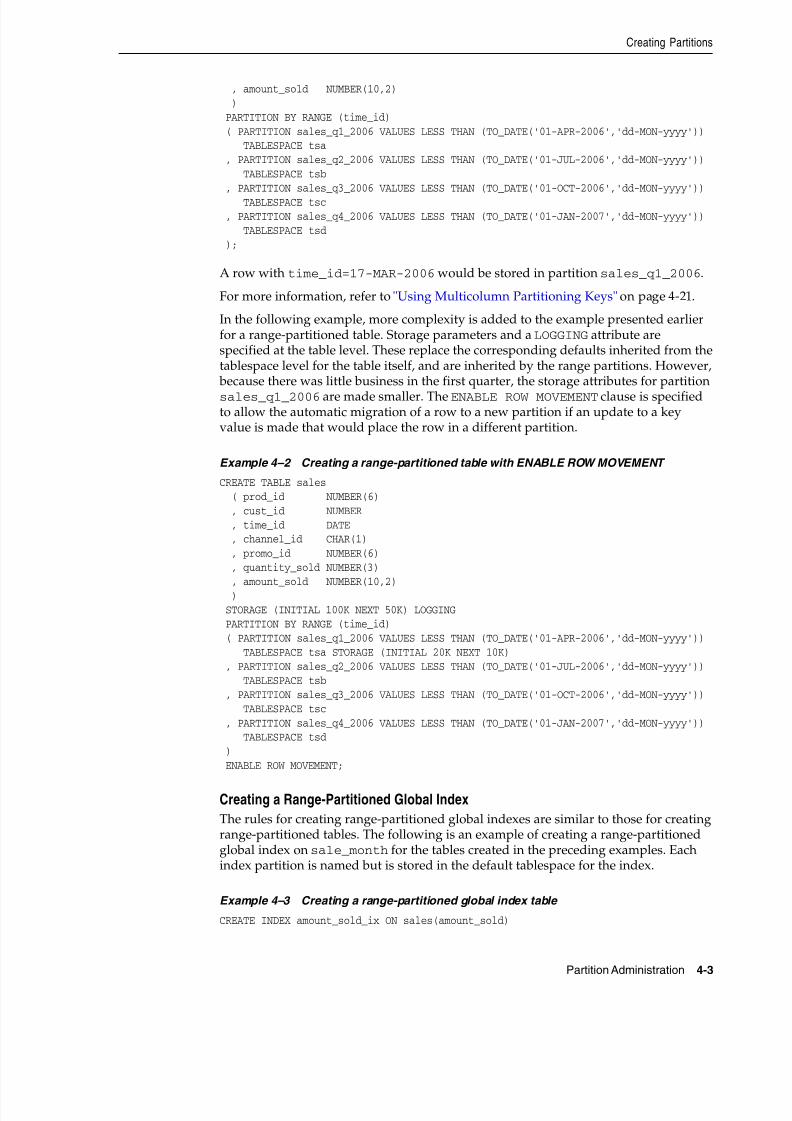
8/16/2019 Oracle Database VLDB and Partitioning Guide
http://slidepdf.com/reader/full/oracle-database-vldb-and-partitioning-guide 81/304
Creating Partitions
Partition Administration 4-3
, amount_sold NUMBER(10,2) ) PARTITION BY RANGE (time_id) ( PARTITION sales_q1_2006 VALUES LESS THAN (TO_DATE('01-APR-2006','dd-MON-yyyy')) TABLESPACE tsa , PARTITION sales_q2_2006 VALUES LESS THAN (TO_DATE('01-JUL-2006','dd-MON-yyyy')) TABLESPACE tsb , PARTITION sales_q3_2006 VALUES LESS THAN (TO_DATE('01-OCT-2006','dd-MON-yyyy')) TABLESPACE tsc , PARTITION sales_q4_2006 VALUES LESS THAN (TO_DATE('01-JAN-2007','dd-MON-yyyy')) TABLESPACE tsd );
A row with time_id=17-MAR-2006 would be stored in partition sales_q1_2006.
For more information, refer to "Using Multicolumn Partitioning Keys" on page 4-21.
In the following example, more complexity is added to the example presented earlierfor a range-partitioned table. Storage parameters and a LOGGING attribute arespecified at the table level. These replace the corresponding defaults inherited from thetablespace level for the table itself, and are inherited by the range partitions. However, because there was little business in the first quarter, the storage attributes for partition
sales_q1_2006 are made smaller. The ENABLE ROW MOVEMENT clause is specifiedto allow the automatic migration of a row to a new partition if an update to a keyvalue is made that would place the row in a different partition.
Example 4–2 Creating a range-partitioned table with ENABLE ROW MOVEMENT
CREATE TABLE sales ( prod_id NUMBER(6) , cust_id NUMBER , time_id DATE , channel_id CHAR(1) , promo_id NUMBER(6) , quantity_sold NUMBER(3) , amount_sold NUMBER(10,2) ) STORAGE (INITIAL 100K NEXT 50K) LOGGING PARTITION BY RANGE (time_id) ( PARTITION sales_q1_2006 VALUES LESS THAN (TO_DATE('01-APR-2006','dd-MON-yyyy')) TABLESPACE tsa STORAGE (INITIAL 20K NEXT 10K) , PARTITION sales_q2_2006 VALUES LESS THAN (TO_DATE('01-JUL-2006','dd-MON-yyyy')) TABLESPACE tsb , PARTITION sales_q3_2006 VALUES LESS THAN (TO_DATE('01-OCT-2006','dd-MON-yyyy')) TABLESPACE tsc , PARTITION sales_q4_2006 VALUES LESS THAN (TO_DATE('01-JAN-2007','dd-MON-yyyy')) TABLESPACE tsd ) ENABLE ROW MOVEMENT;
Creating a Range-Partitioned Global Index
The rules for creating range-partitioned global indexes are similar to those for creatingrange-partitioned tables. The following is an example of creating a range-partitionedglobal index on sale_month for the tables created in the preceding examples. Eachindex partition is named but is stored in the default tablespace for the index.
Example 4–3 Creating a range-partitioned global index table
CREATE INDEX amount_sold_ix ON sales(amount_sold)
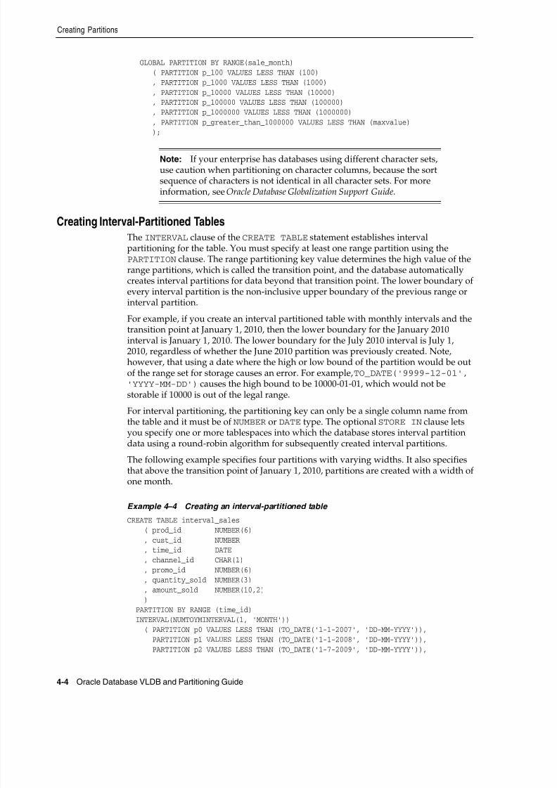
8/16/2019 Oracle Database VLDB and Partitioning Guide
http://slidepdf.com/reader/full/oracle-database-vldb-and-partitioning-guide 82/304
Creating Partitions
4-4 Oracle Database VLDB and Partitioning Guide
GLOBAL PARTITION BY RANGE(sale_month) ( PARTITION p_100 VALUES LESS THAN (100) , PARTITION p_1000 VALUES LESS THAN (1000) , PARTITION p_10000 VALUES LESS THAN (10000) , PARTITION p_100000 VALUES LESS THAN (100000) , PARTITION p_1000000 VALUES LESS THAN (1000000) , PARTITION p_greater_than_1000000 VALUES LESS THAN (maxvalue) );
Creating Interval-Partitioned TablesThe INTERVAL clause of the CREATE TABLE statement establishes intervalpartitioning for the table. You must specify at least one range partition using thePARTITION clause. The range partitioning key value determines the high value of therange partitions, which is called the transition point, and the database automaticallycreates interval partitions for data beyond that transition point. The lower boundary ofevery interval partition is the non-inclusive upper boundary of the previous range orinterval partition.
For example, if you create an interval partitioned table with monthly intervals and thetransition point at January 1, 2010, then the lower boundary for the January 2010interval is January 1, 2010. The lower boundary for the July 2010 interval is July 1,2010, regardless of whether the June 2010 partition was previously created. Note,however, that using a date where the high or low bound of the partition would be outof the range set for storage causes an error. For example, TO_DATE('9999-12-01','YYYY-MM-DD') causes the high bound to be 10000-01-01, which would not bestorable if 10000 is out of the legal range.
For interval partitioning, the partitioning key can only be a single column name fromthe table and it must be of NUMBER or DATE type. The optional STORE IN clause letsyou specify one or more tablespaces into which the database stores interval partitiondata using a round-robin algorithm for subsequently created interval partitions.
The following example specifies four partitions with varying widths. It also specifiesthat above the transition point of January 1, 2010, partitions are created with a width ofone month.
Example 4–4 Creating an interval-partitioned table
CREATE TABLE interval_sales ( prod_id NUMBER(6) , cust_id NUMBER
, time_id DATE , channel_id CHAR(1) , promo_id NUMBER(6) , quantity_sold NUMBER(3) , amount_sold NUMBER(10,2) )PARTITION BY RANGE (time_id)INTERVAL(NUMTOYMINTERVAL(1, 'MONTH'))
( PARTITION p0 VALUES LESS THAN (TO_DATE('1-1-2007', 'DD-MM-YYYY')), PARTITION p1 VALUES LESS THAN (TO_DATE('1-1-2008', 'DD-MM-YYYY')), PARTITION p2 VALUES LESS THAN (TO_DATE('1-7-2009', 'DD-MM-YYYY')),
Note: If your enterprise has databases using different character sets,use caution when partitioning on character columns, because the sortsequence of characters is not identical in all character sets. For moreinformation, see Oracle Database Globalization Support Guide.

8/16/2019 Oracle Database VLDB and Partitioning Guide
http://slidepdf.com/reader/full/oracle-database-vldb-and-partitioning-guide 83/304
Creating Partitions
Partition Administration 4-5
PARTITION p3 VALUES LESS THAN (TO_DATE('1-1-2010', 'DD-MM-YYYY')) );
The high bound of partition p3 represents the transition point. p3 and all partitions below it (p0, p1, and p2 in this example) are in the range section while all partitionsabove it fall into the interval section.
Creating Hash-Partitioned Tables and Global IndexesThe PARTITION BY HASH clause of the CREATE TABLE statement identifies that thetable is to be hash-partitioned. The PARTITIONS clause can then be used to specify thenumber of partitions to create, and optionally, the tablespaces to store them in.Alternatively, you can use PARTITION clauses to name the individual partitions andtheir tablespaces.
The only attribute you can specify for hash partitions is TABLESPACE. All of the hashpartitions of a table must share the same segment attributes (except TABLESPACE),which are inherited from the table level.
Creating a Hash Partitioned Table
The following example creates a hash-partitioned table. The partitioning column is id,
four partitions are created and assigned system generated names, and they are placedin four named tablespaces (gear1, gear2, ...).
Example 4–5 Creating a hash-partitioned table
CREATE TABLE scubagear (id NUMBER, name VARCHAR2 (60)) PARTITION BY HASH (id) PARTITIONS 4
STORE IN (gear1, gear2, gear3, gear4);
For more information, refer to "Using Multicolumn Partitioning Keys" on page 4-21.
The following examples illustrate two methods of creating a hash-partitioned tablenamed dept. In the first example the number of partitions is specified, but systemgenerated names are assigned to them and they are stored in the default tablespace ofthe table.
CREATE TABLE dept (deptno NUMBER, deptname VARCHAR(32)) PARTITION BY HASH(deptno) PARTITIONS 16;
In the following example, names of individual partitions, and tablespaces in whichthey are to reside, are specified. The initial extent size for each hash partition (segment)is also explicitly stated at the table level, and all partitions inherit this attribute.
CREATE TABLE dept (deptno NUMBER, deptname VARCHAR(32)) STORAGE (INITIAL 10K)
PARTITION BY HASH(deptno) (PARTITION p1 TABLESPACE ts1, PARTITION p2 TABLESPACE ts2, PARTITION p3 TABLESPACE ts1, PARTITION p4 TABLESPACE ts3);
If you create a local index for this table, the database constructs the index so that it isequipartitioned with the underlying table. The database also ensures that the index ismaintained automatically when maintenance operations are performed on theunderlying table. The following is an example of creating a local index on the tabledept:
CREATE INDEX loc_dept_ix ON dept(deptno) LOCAL;
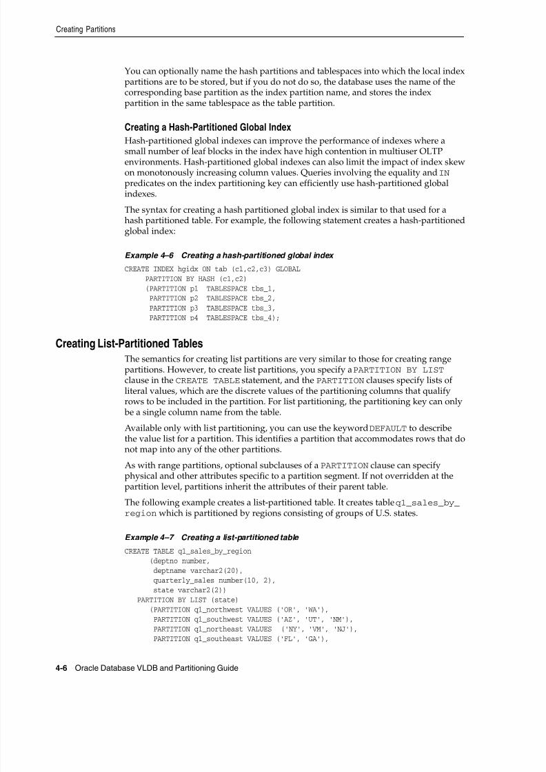
8/16/2019 Oracle Database VLDB and Partitioning Guide
http://slidepdf.com/reader/full/oracle-database-vldb-and-partitioning-guide 84/304
Creating Partitions
4-6 Oracle Database VLDB and Partitioning Guide
You can optionally name the hash partitions and tablespaces into which the local indexpartitions are to be stored, but if you do not do so, the database uses the name of thecorresponding base partition as the index partition name, and stores the indexpartition in the same tablespace as the table partition.
Creating a Hash-Partitioned Global Index
Hash-partitioned global indexes can improve the performance of indexes where asmall number of leaf blocks in the index have high contention in multiuser OLTPenvironments. Hash-partitioned global indexes can also limit the impact of index skewon monotonously increasing column values. Queries involving the equality and IN predicates on the index partitioning key can efficiently use hash-partitioned globalindexes.
The syntax for creating a hash partitioned global index is similar to that used for ahash partitioned table. For example, the following statement creates a hash-partitionedglobal index:
Example 4–6 Creating a hash-partitioned global index
CREATE INDEX hgidx ON tab (c1,c2,c3) GLOBAL PARTITION BY HASH (c1,c2) (PARTITION p1 TABLESPACE tbs_1, PARTITION p2 TABLESPACE tbs_2, PARTITION p3 TABLESPACE tbs_3, PARTITION p4 TABLESPACE tbs_4);
Creating List-Partitioned TablesThe semantics for creating list partitions are very similar to those for creating rangepartitions. However, to create list partitions, you specify a PARTITION BY LIST clause in the CREATE TABLE statement, and the PARTITION clauses specify lists ofliteral values, which are the discrete values of the partitioning columns that qualify
rows to be included in the partition. For list partitioning, the partitioning key can only be a single column name from the table.
Available only with list partitioning, you can use the keyword DEFAULT to describethe value list for a partition. This identifies a partition that accommodates rows that donot map into any of the other partitions.
As with range partitions, optional subclauses of a PARTITION clause can specifyphysical and other attributes specific to a partition segment. If not overridden at thepartition level, partitions inherit the attributes of their parent table.
The following example creates a list-partitioned table. It creates table q1_sales_by_region which is partitioned by regions consisting of groups of U.S. states.
Example 4–7 Creating a list-partitioned table CREATE TABLE q1_sales_by_region (deptno number,
deptname varchar2(20), quarterly_sales number(10, 2), state varchar2(2)) PARTITION BY LIST (state) (PARTITION q1_northwest VALUES ('OR', 'WA'), PARTITION q1_southwest VALUES ('AZ', 'UT', 'NM'), PARTITION q1_northeast VALUES ('NY', 'VM', 'NJ'), PARTITION q1_southeast VALUES ('FL', 'GA'),
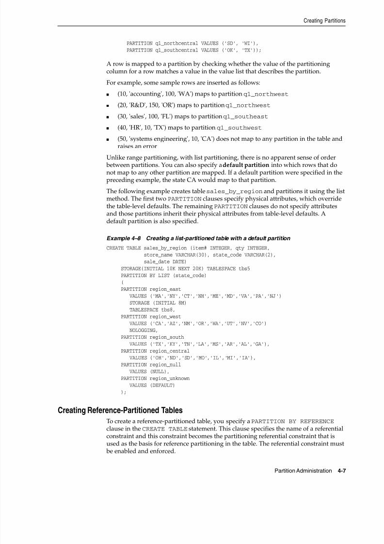
8/16/2019 Oracle Database VLDB and Partitioning Guide
http://slidepdf.com/reader/full/oracle-database-vldb-and-partitioning-guide 85/304
Creating Partitions
Partition Administration 4-7
PARTITION q1_northcentral VALUES ('SD', 'WI'), PARTITION q1_southcentral VALUES ('OK', 'TX'));
A row is mapped to a partition by checking whether the value of the partitioningcolumn for a row matches a value in the value list that describes the partition.
For example, some sample rows are inserted as follows:
■ (10, 'accounting', 100, 'WA') maps to partition q1_northwest■ (20, 'R&D', 150, 'OR') maps to partition q1_northwest
■ (30, 'sales', 100, 'FL') maps to partition q1_southeast
■ (40, 'HR', 10, 'TX') maps to partition q1_southwest
■ (50, 'systems engineering', 10, 'CA') does not map to any partition in the table andraises an error
Unlike range partitioning, with list partitioning, there is no apparent sense of order between partitions. You can also specify a default partition into which rows that donot map to any other partition are mapped. If a default partition were specified in thepreceding example, the state CA would map to that partition.
The following example creates table sales_by_region and partitions it using the listmethod. The first two PARTITION clauses specify physical attributes, which overridethe table-level defaults. The remaining PARTITION clauses do not specify attributesand those partitions inherit their physical attributes from table-level defaults. Adefault partition is also specified.
Example 4–8 Creating a list-partitioned table with a default partition
CREATE TABLE sales_by_region (item# INTEGER, qty INTEGER,store_name VARCHAR(30), state_code VARCHAR(2),
sale_date DATE) STORAGE(INITIAL 10K NEXT 20K) TABLESPACE tbs5
PARTITION BY LIST (state_code)(
PARTITION region_east VALUES ('MA','NY','CT','NH','ME','MD','VA','PA','NJ') STORAGE (INITIAL 8M)
TABLESPACE tbs8, PARTITION region_west VALUES ('CA','AZ','NM','OR','WA','UT','NV','CO') NOLOGGING, PARTITION region_south VALUES ('TX','KY','TN','LA','MS','AR','AL','GA'), PARTITION region_central
VALUES ('OH','ND','SD','MO','IL','MI','IA'), PARTITION region_null VALUES (NULL),
PARTITION region_unknown VALUES (DEFAULT) );
Creating Reference-Partitioned TablesTo create a reference-partitioned table, you specify a PARTITION BY REFERENCE clause in the CREATE TABLE statement. This clause specifies the name of a referentialconstraint and this constraint becomes the partitioning referential constraint that isused as the basis for reference partitioning in the table. The referential constraint must be enabled and enforced.
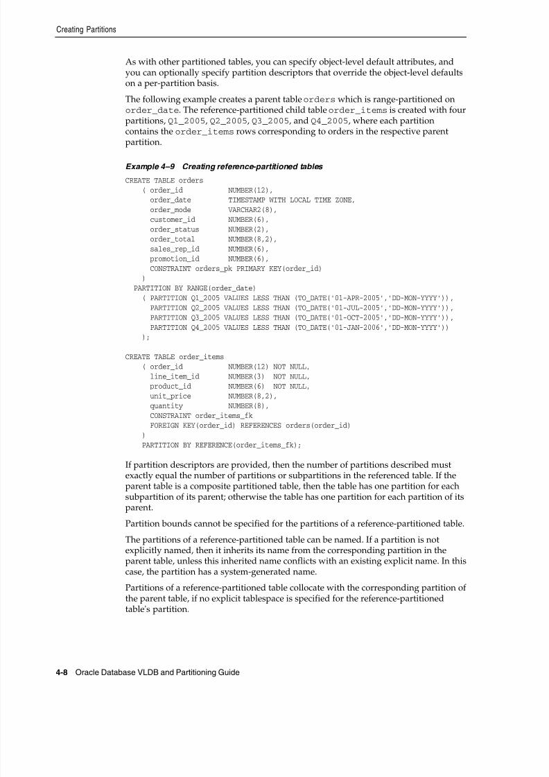
8/16/2019 Oracle Database VLDB and Partitioning Guide
http://slidepdf.com/reader/full/oracle-database-vldb-and-partitioning-guide 86/304
Creating Partitions
4-8 Oracle Database VLDB and Partitioning Guide
As with other partitioned tables, you can specify object-level default attributes, andyou can optionally specify partition descriptors that override the object-level defaultson a per-partition basis.
The following example creates a parent table orders which is range-partitioned onorder_date. The reference-partitioned child table order_items is created with fourpartitions, Q1_2005, Q2_2005, Q3_2005, and Q4_2005, where each partition
contains the order_items rows corresponding to orders in the respective parentpartition.
Example 4–9 Creating reference-partitioned tables
CREATE TABLE orders ( order_id NUMBER(12), order_date TIMESTAMP WITH LOCAL TIME ZONE, order_mode VARCHAR2(8), customer_id NUMBER(6), order_status NUMBER(2), order_total NUMBER(8,2), sales_rep_id NUMBER(6), promotion_id NUMBER(6),
CONSTRAINT orders_pk PRIMARY KEY(order_id) ) PARTITION BY RANGE(order_date) ( PARTITION Q1_2005 VALUES LESS THAN (TO_DATE('01-APR-2005','DD-MON-YYYY')), PARTITION Q2_2005 VALUES LESS THAN (TO_DATE('01-JUL-2005','DD-MON-YYYY')), PARTITION Q3_2005 VALUES LESS THAN (TO_DATE('01-OCT-2005','DD-MON-YYYY')), PARTITION Q4_2005 VALUES LESS THAN (TO_DATE('01-JAN-2006','DD-MON-YYYY')) );
CREATE TABLE order_items ( order_id NUMBER(12) NOT NULL, line_item_id NUMBER(3) NOT NULL, product_id NUMBER(6) NOT NULL, unit_price NUMBER(8,2),
quantity NUMBER(8), CONSTRAINT order_items_fk FOREIGN KEY(order_id) REFERENCES orders(order_id) ) PARTITION BY REFERENCE(order_items_fk);
If partition descriptors are provided, then the number of partitions described mustexactly equal the number of partitions or subpartitions in the referenced table. If theparent table is a composite partitioned table, then the table has one partition for eachsubpartition of its parent; otherwise the table has one partition for each partition of itsparent.
Partition bounds cannot be specified for the partitions of a reference-partitioned table.
The partitions of a reference-partitioned table can be named. If a partition is notexplicitly named, then it inherits its name from the corresponding partition in theparent table, unless this inherited name conflicts with an existing explicit name. In thiscase, the partition has a system-generated name.
Partitions of a reference-partitioned table collocate with the corresponding partition ofthe parent table, if no explicit tablespace is specified for the reference-partitionedtable's partition.
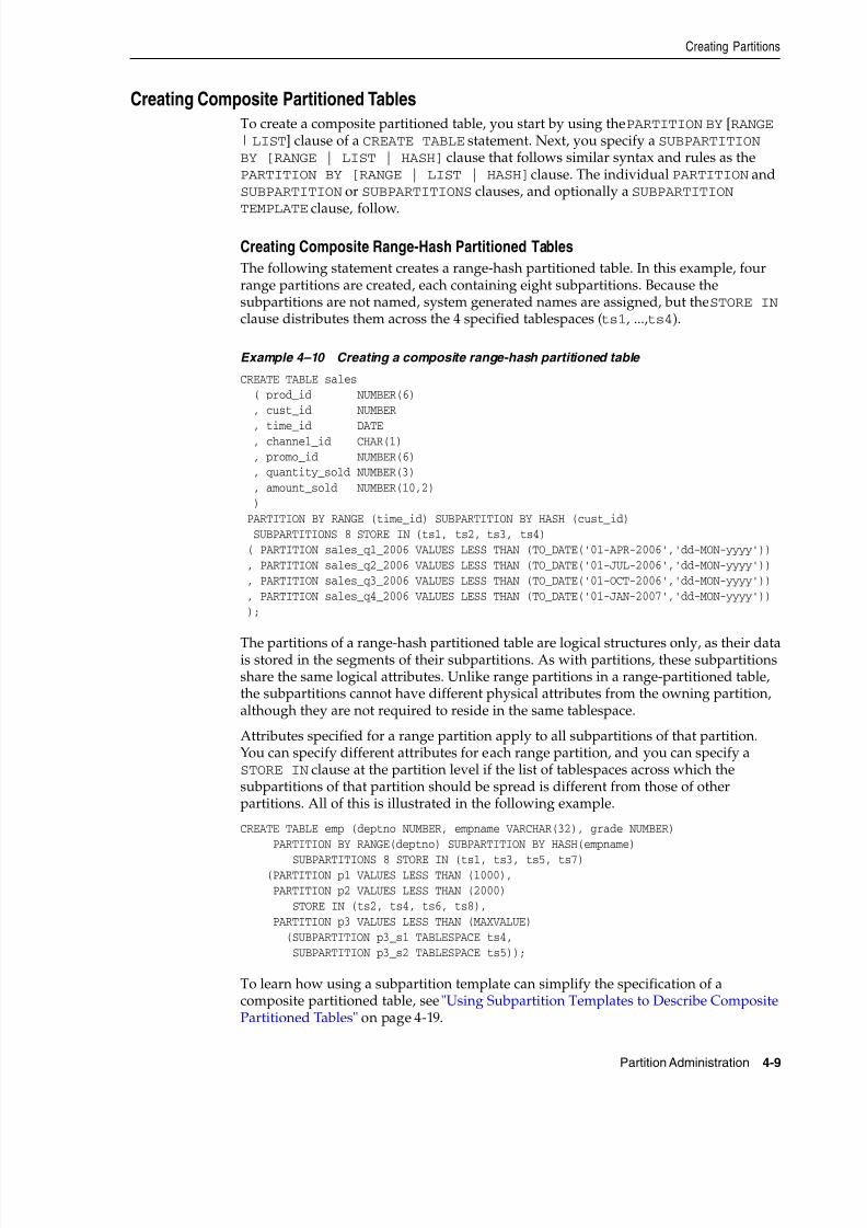
8/16/2019 Oracle Database VLDB and Partitioning Guide
http://slidepdf.com/reader/full/oracle-database-vldb-and-partitioning-guide 87/304
Creating Partitions
Partition Administration 4-9
Creating Composite Partitioned TablesTo create a composite partitioned table, you start by using the PARTITION BY [RANGE | LIST] clause of a CREATE TABLE statement. Next, you specify a SUBPARTITIONBY [RANGE | LIST | HASH] clause that follows similar syntax and rules as thePARTITION BY [RANGE | LIST | HASH] clause. The individual PARTITION andSUBPARTITION or SUBPARTITIONS clauses, and optionally a SUBPARTITION
TEMPLATE clause, follow.
Creating Composite Range-Hash Partitioned Tables
The following statement creates a range-hash partitioned table. In this example, fourrange partitions are created, each containing eight subpartitions. Because thesubpartitions are not named, system generated names are assigned, but the STORE IN clause distributes them across the 4 specified tablespaces (ts1, ...,ts4).
Example 4–10 Creating a composite range-hash partitioned table
CREATE TABLE sales ( prod_id NUMBER(6) , cust_id NUMBER
, time_id DATE , channel_id CHAR(1) , promo_id NUMBER(6) , quantity_sold NUMBER(3) , amount_sold NUMBER(10,2) ) PARTITION BY RANGE (time_id) SUBPARTITION BY HASH (cust_id) SUBPARTITIONS 8 STORE IN (ts1, ts2, ts3, ts4) ( PARTITION sales_q1_2006 VALUES LESS THAN (TO_DATE('01-APR-2006','dd-MON-yyyy')) , PARTITION sales_q2_2006 VALUES LESS THAN (TO_DATE('01-JUL-2006','dd-MON-yyyy')) , PARTITION sales_q3_2006 VALUES LESS THAN (TO_DATE('01-OCT-2006','dd-MON-yyyy')) , PARTITION sales_q4_2006 VALUES LESS THAN (TO_DATE('01-JAN-2007','dd-MON-yyyy')) );
The partitions of a range-hash partitioned table are logical structures only, as their datais stored in the segments of their subpartitions. As with partitions, these subpartitionsshare the same logical attributes. Unlike range partitions in a range-partitioned table,the subpartitions cannot have different physical attributes from the owning partition,although they are not required to reside in the same tablespace.
Attributes specified for a range partition apply to all subpartitions of that partition.You can specify different attributes for each range partition, and you can specify aSTORE IN clause at the partition level if the list of tablespaces across which thesubpartitions of that partition should be spread is different from those of otherpartitions. All of this is illustrated in the following example.
CREATE TABLE emp (deptno NUMBER, empname VARCHAR(32), grade NUMBER)PARTITION BY RANGE(deptno) SUBPARTITION BY HASH(empname)
SUBPARTITIONS 8 STORE IN (ts1, ts3, ts5, ts7) (PARTITION p1 VALUES LESS THAN (1000), PARTITION p2 VALUES LESS THAN (2000) STORE IN (ts2, ts4, ts6, ts8), PARTITION p3 VALUES LESS THAN (MAXVALUE) (SUBPARTITION p3_s1 TABLESPACE ts4, SUBPARTITION p3_s2 TABLESPACE ts5));
To learn how using a subpartition template can simplify the specification of acomposite partitioned table, see "Using Subpartition Templates to Describe CompositePartitioned Tables" on page 4-19.

8/16/2019 Oracle Database VLDB and Partitioning Guide
http://slidepdf.com/reader/full/oracle-database-vldb-and-partitioning-guide 88/304
Creating Partitions
4-10 Oracle Database VLDB and Partitioning Guide
The following statement is an example of creating a local index on the emp table wherethe index segments are spread across tablespaces ts7, ts8, and ts9.
CREATE INDEX emp_ix ON emp(deptno) LOCAL STORE IN (ts7, ts8, ts9);
This local index is equipartitioned with the base table as follows:
■ It consists of as many partitions as the base table.■ Each index partition consists of as many subpartitions as the corresponding base
table partition.
■ Index entries for rows in a given subpartition of the base table are stored in thecorresponding subpartition of the index.
Creating Composite Range-List Partitioned Tables
The range partitions of a range-list composite partitioned table are described as fornon-composite range partitioned tables. This allows that optional subclauses of aPARTITION clause can specify physical and other attributes, including tablespace,specific to a partition segment. If not overridden at the partition level, partitions
inherit the attributes of their underlying table.The list subpartition descriptions, in the SUBPARTITION clauses, are described as fornon-composite list partitions, except the only physical attribute that can be specified isa tablespace (optional). Subpartitions inherit all other physical attributes from thepartition description.
The following example illustrates how range-list partitioning might be used. Theexample tracks sales data of products by quarters and within each quarter, groups it by specified states.
Example 4–11 Creating a composite range-list partitioned table
CREATE TABLE quarterly_regional_sales (deptno number, item_no varchar2(20),
txn_date date, txn_amount number, state varchar2(2)) TABLESPACE ts4 PARTITION BY RANGE (txn_date) SUBPARTITION BY LIST (state) (PARTITION q1_1999 VALUES LESS THAN (TO_DATE('1-APR-1999','DD-MON-YYYY')) (SUBPARTITION q1_1999_northwest VALUES ('OR', 'WA'), SUBPARTITION q1_1999_southwest VALUES ('AZ', 'UT', 'NM'), SUBPARTITION q1_1999_northeast VALUES ('NY', 'VM', 'NJ'), SUBPARTITION q1_1999_southeast VALUES ('FL', 'GA'), SUBPARTITION q1_1999_northcentral VALUES ('SD', 'WI'), SUBPARTITION q1_1999_southcentral VALUES ('OK', 'TX') ), PARTITION q2_1999 VALUES LESS THAN ( TO_DATE('1-JUL-1999','DD-MON-YYYY')) (SUBPARTITION q2_1999_northwest VALUES ('OR', 'WA'), SUBPARTITION q2_1999_southwest VALUES ('AZ', 'UT', 'NM'), SUBPARTITION q2_1999_northeast VALUES ('NY', 'VM', 'NJ'), SUBPARTITION q2_1999_southeast VALUES ('FL', 'GA'), SUBPARTITION q2_1999_northcentral VALUES ('SD', 'WI'), SUBPARTITION q2_1999_southcentral VALUES ('OK', 'TX') ), PARTITION q3_1999 VALUES LESS THAN (TO_DATE('1-OCT-1999','DD-MON-YYYY')) (SUBPARTITION q3_1999_northwest VALUES ('OR', 'WA'), SUBPARTITION q3_1999_southwest VALUES ('AZ', 'UT', 'NM'), SUBPARTITION q3_1999_northeast VALUES ('NY', 'VM', 'NJ'), SUBPARTITION q3_1999_southeast VALUES ('FL', 'GA'),
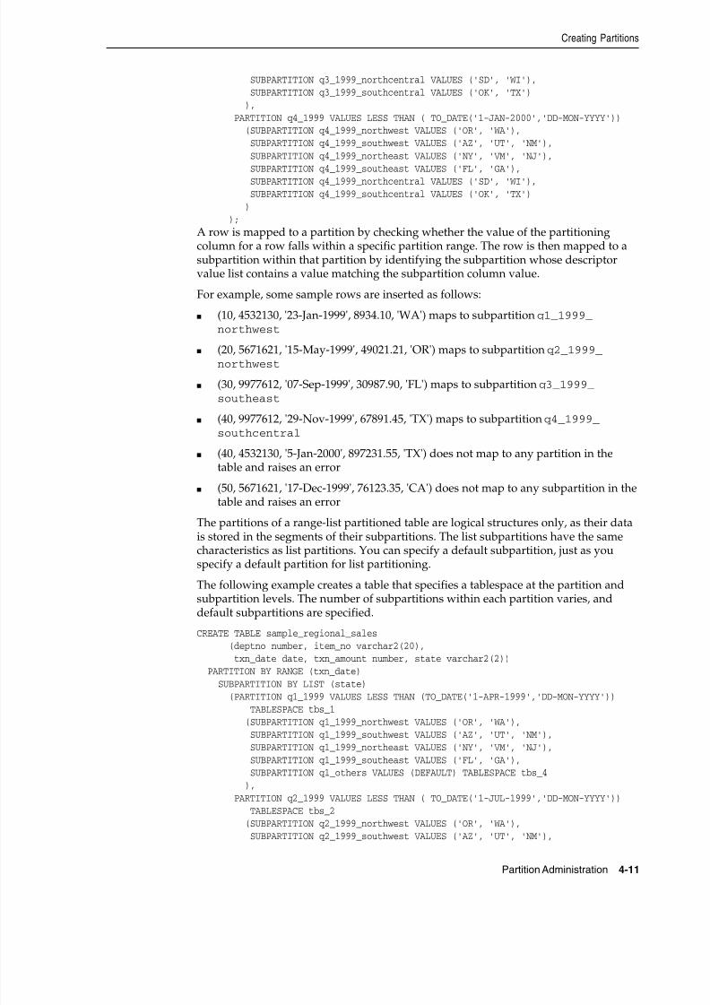
8/16/2019 Oracle Database VLDB and Partitioning Guide
http://slidepdf.com/reader/full/oracle-database-vldb-and-partitioning-guide 89/304
Creating Partitions
Partition Administration 4-11
SUBPARTITION q3_1999_northcentral VALUES ('SD', 'WI'), SUBPARTITION q3_1999_southcentral VALUES ('OK', 'TX') ), PARTITION q4_1999 VALUES LESS THAN ( TO_DATE('1-JAN-2000','DD-MON-YYYY')) (SUBPARTITION q4_1999_northwest VALUES ('OR', 'WA'), SUBPARTITION q4_1999_southwest VALUES ('AZ', 'UT', 'NM'), SUBPARTITION q4_1999_northeast VALUES ('NY', 'VM', 'NJ'), SUBPARTITION q4_1999_southeast VALUES ('FL', 'GA'), SUBPARTITION q4_1999_northcentral VALUES ('SD', 'WI'), SUBPARTITION q4_1999_southcentral VALUES ('OK', 'TX') ) );
A row is mapped to a partition by checking whether the value of the partitioningcolumn for a row falls within a specific partition range. The row is then mapped to asubpartition within that partition by identifying the subpartition whose descriptorvalue list contains a value matching the subpartition column value.
For example, some sample rows are inserted as follows:
■ (10, 4532130, '23-Jan-1999', 8934.10, 'WA') maps to subpartition q1_1999_northwest
■ (20, 5671621, '15-May-1999', 49021.21, 'OR') maps to subpartition q2_1999_northwest
■ (30, 9977612, '07-Sep-1999', 30987.90, 'FL') maps to subpartition q3_1999_southeast
■ (40, 9977612, '29-Nov-1999', 67891.45, 'TX') maps to subpartition q4_1999_southcentral
■ (40, 4532130, '5-Jan-2000', 897231.55, 'TX') does not map to any partition in thetable and raises an error
■ (50, 5671621, '17-Dec-1999', 76123.35, 'CA') does not map to any subpartition in thetable and raises an error
The partitions of a range-list partitioned table are logical structures only, as their datais stored in the segments of their subpartitions. The list subpartitions have the samecharacteristics as list partitions. You can specify a default subpartition, just as youspecify a default partition for list partitioning.
The following example creates a table that specifies a tablespace at the partition andsubpartition levels. The number of subpartitions within each partition varies, anddefault subpartitions are specified.
CREATE TABLE sample_regional_sales (deptno number, item_no varchar2(20), txn_date date, txn_amount number, state varchar2(2)) PARTITION BY RANGE (txn_date) SUBPARTITION BY LIST (state) (PARTITION q1_1999 VALUES LESS THAN (TO_DATE('1-APR-1999','DD-MON-YYYY')) TABLESPACE tbs_1 (SUBPARTITION q1_1999_northwest VALUES ('OR', 'WA'), SUBPARTITION q1_1999_southwest VALUES ('AZ', 'UT', 'NM'), SUBPARTITION q1_1999_northeast VALUES ('NY', 'VM', 'NJ'), SUBPARTITION q1_1999_southeast VALUES ('FL', 'GA'), SUBPARTITION q1_others VALUES (DEFAULT) TABLESPACE tbs_4 ), PARTITION q2_1999 VALUES LESS THAN ( TO_DATE('1-JUL-1999','DD-MON-YYYY')) TABLESPACE tbs_2 (SUBPARTITION q2_1999_northwest VALUES ('OR', 'WA'), SUBPARTITION q2_1999_southwest VALUES ('AZ', 'UT', 'NM'),
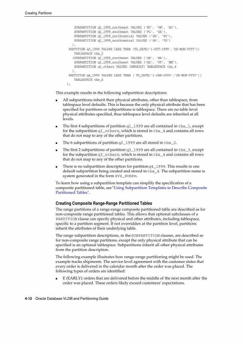
8/16/2019 Oracle Database VLDB and Partitioning Guide
http://slidepdf.com/reader/full/oracle-database-vldb-and-partitioning-guide 90/304
Creating Partitions
4-12 Oracle Database VLDB and Partitioning Guide
SUBPARTITION q2_1999_northeast VALUES ('NY', 'VM', 'NJ'), SUBPARTITION q2_1999_southeast VALUES ('FL', 'GA'), SUBPARTITION q2_1999_northcentral VALUES ('SD', 'WI'), SUBPARTITION q2_1999_southcentral VALUES ('OK', 'TX') ), PARTITION q3_1999 VALUES LESS THAN (TO_DATE('1-OCT-1999','DD-MON-YYYY')) TABLESPACE tbs_3 (SUBPARTITION q3_1999_northwest VALUES ('OR', 'WA'), SUBPARTITION q3_1999_southwest VALUES ('AZ', 'UT', 'NM'), SUBPARTITION q3_others VALUES (DEFAULT) TABLESPACE tbs_4 ), PARTITION q4_1999 VALUES LESS THAN ( TO_DATE('1-JAN-2000','DD-MON-YYYY')) TABLESPACE tbs_4 );
This example results in the following subpartition descriptions:
■ All subpartitions inherit their physical attributes, other than tablespace, fromtablespace level defaults. This is because the only physical attribute that has beenspecified for partitions or subpartitions is tablespace. There are no table levelphysical attributes specified, thus tablespace level defaults are inherited at all
levels.■ The first 4 subpartitions of partition q1_1999 are all contained in tbs_1, except
for the subpartition q1_others, which is stored in tbs_4 and contains all rowsthat do not map to any of the other partitions.
■ The 6 subpartitions of partition q2_1999 are all stored in tbs_2.
■ The first 2 subpartitions of partition q3_1999 are all contained in tbs_3, exceptfor the subpartition q3_others, which is stored in tbs_4 and contains all rowsthat do not map to any of the other partitions.
■ There is no subpartition description for partition q4_1999. This results in onedefault subpartition being created and stored in tbs_4. The subpartition name issystem generated in the form SYS_SUBPn.
To learn how using a subpartition template can simplify the specification of acomposite partitioned table, see "Using Subpartition Templates to Describe CompositePartitioned Tables".
Creating Composite Range-Range Partitioned Tables
The range partitions of a range-range composite partitioned table are described as fornon-composite range partitioned tables. This allows that optional subclauses of aPARTITION clause can specify physical and other attributes, including tablespace,specific to a partition segment. If not overridden at the partition level, partitionsinherit the attributes of their underlying table.
The range subpartition descriptions, in the SUBPARTITION clauses, are described as
for non-composite range partitions, except the only physical attribute that can bespecified is an optional tablespace. Subpartitions inherit all other physical attributesfrom the partition description.
The following example illustrates how range-range partitioning might be used. Theexample tracks shipments. The service level agreement with the customer states thatevery order is delivered in the calendar month after the order was placed. Thefollowing types of orders are identified:
■ E (EARLY): orders that are delivered before the middle of the next month after theorder was placed. These orders likely exceed customers' expectations.
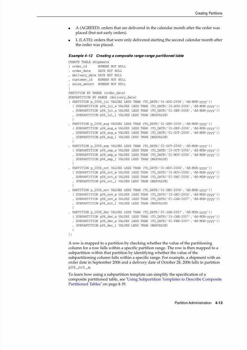
8/16/2019 Oracle Database VLDB and Partitioning Guide
http://slidepdf.com/reader/full/oracle-database-vldb-and-partitioning-guide 91/304
Creating Partitions
Partition Administration 4-13
■ A (AGREED): orders that are delivered in the calendar month after the order wasplaced (but not early orders).
■ L (LATE): orders that were only delivered starting the second calendar month afterthe order was placed.
Example 4–12 Creating a composite range-range partitioned table
CREATE TABLE shipments( order_id NUMBER NOT NULL, order_date DATE NOT NULL, delivery_date DATE NOT NULL, customer_id NUMBER NOT NULL, sales_amount NUMBER NOT NULL)PARTITION BY RANGE (order_date)SUBPARTITION BY RANGE (delivery_date)( PARTITION p_2006_jul VALUES LESS THAN (TO_DATE('01-AUG-2006','dd-MON-yyyy')) ( SUBPARTITION p06_jul_e VALUES LESS THAN (TO_DATE('15-AUG-2006','dd-MON-yyyy')) , SUBPARTITION p06_jul_a VALUES LESS THAN (TO_DATE('01-SEP-2006','dd-MON-yyyy')) , SUBPARTITION p06_jul_l VALUES LESS THAN (MAXVALUE) )
, PARTITION p_2006_aug VALUES LESS THAN (TO_DATE('01-SEP-2006','dd-MON-yyyy')) ( SUBPARTITION p06_aug_e VALUES LESS THAN (TO_DATE('15-SEP-2006','dd-MON-yyyy')) , SUBPARTITION p06_aug_a VALUES LESS THAN (TO_DATE('01-OCT-2006','dd-MON-yyyy')) , SUBPARTITION p06_aug_l VALUES LESS THAN (MAXVALUE) ), PARTITION p_2006_sep VALUES LESS THAN (TO_DATE('01-OCT-2006','dd-MON-yyyy')) ( SUBPARTITION p06_sep_e VALUES LESS THAN (TO_DATE('15-OCT-2006','dd-MON-yyyy')) , SUBPARTITION p06_sep_a VALUES LESS THAN (TO_DATE('01-NOV-2006','dd-MON-yyyy')) , SUBPARTITION p06_sep_l VALUES LESS THAN (MAXVALUE) ), PARTITION p_2006_oct VALUES LESS THAN (TO_DATE('01-NOV-2006','dd-MON-yyyy')) ( SUBPARTITION p06_oct_e VALUES LESS THAN (TO_DATE('15-NOV-2006','dd-MON-yyyy')) , SUBPARTITION p06_oct_a VALUES LESS THAN (TO_DATE('01-DEC-2006','dd-MON-yyyy')) , SUBPARTITION p06_oct_l VALUES LESS THAN (MAXVALUE) ), PARTITION p_2006_nov VALUES LESS THAN (TO_DATE('01-DEC-2006','dd-MON-yyyy')) ( SUBPARTITION p06_nov_e VALUES LESS THAN (TO_DATE('15-DEC-2006','dd-MON-yyyy')) , SUBPARTITION p06_nov_a VALUES LESS THAN (TO_DATE('01-JAN-2007','dd-MON-yyyy')) , SUBPARTITION p06_nov_l VALUES LESS THAN (MAXVALUE) ), PARTITION p_2006_dec VALUES LESS THAN (TO_DATE('01-JAN-2007','dd-MON-yyyy')) ( SUBPARTITION p06_dec_e VALUES LESS THAN (TO_DATE('15-JAN-2007','dd-MON-yyyy')) , SUBPARTITION p06_dec_a VALUES LESS THAN (TO_DATE('01-FEB-2007','dd-MON-yyyy')) , SUBPARTITION p06_dec_l VALUES LESS THAN (MAXVALUE) ));
A row is mapped to a partition by checking whether the value of the partitioningcolumn for a row falls within a specific partition range. The row is then mapped to asubpartition within that partition by identifying whether the value of thesubpartitioning column falls within a specific range. For example, a shipment with anorder date in September 2006 and a delivery date of October 28, 2006 falls in partitionp06_oct_a.
To learn how using a subpartition template can simplify the specification of acomposite partitioned table, see "Using Subpartition Templates to Describe CompositePartitioned Tables" on page 4-19.
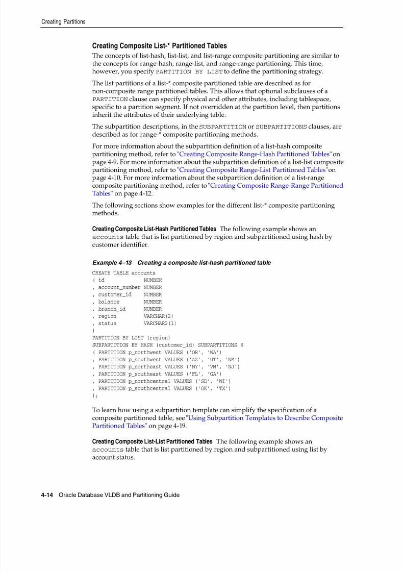
8/16/2019 Oracle Database VLDB and Partitioning Guide
http://slidepdf.com/reader/full/oracle-database-vldb-and-partitioning-guide 92/304
Creating Partitions
4-14 Oracle Database VLDB and Partitioning Guide
Creating Composite List-* Partitioned Tables
The concepts of list-hash, list-list, and list-range composite partitioning are similar tothe concepts for range-hash, range-list, and range-range partitioning. This time,however, you specify PARTITION BY LIST to define the partitioning strategy.
The list partitions of a list-* composite partitioned table are described as fornon-composite range partitioned tables. This allows that optional subclauses of a
PARTITION clause can specify physical and other attributes, including tablespace,specific to a partition segment. If not overridden at the partition level, then partitionsinherit the attributes of their underlying table.
The subpartition descriptions, in the SUBPARTITION or SUBPARTITIONS clauses, aredescribed as for range-* composite partitioning methods.
For more information about the subpartition definition of a list-hash compositepartitioning method, refer to "Creating Composite Range-Hash Partitioned Tables" onpage 4-9. For more information about the subpartition definition of a list-list compositepartitioning method, refer to "Creating Composite Range-List Partitioned Tables" onpage 4-10. For more information about the subpartition definition of a list-rangecomposite partitioning method, refer to "Creating Composite Range-Range PartitionedTables" on page 4-12.
The following sections show examples for the different list-* composite partitioningmethods.
Creating Composite List-Hash Partitioned Tables The following example shows anaccounts table that is list partitioned by region and subpartitioned using hash bycustomer identifier.
Example 4–13 Creating a composite list-hash partitioned table
CREATE TABLE accounts( id NUMBER, account_number NUMBER, customer_id NUMBER
, balance NUMBER, branch_id NUMBER, region VARCHAR(2), status VARCHAR2(1))PARTITION BY LIST (region)SUBPARTITION BY HASH (customer_id) SUBPARTITIONS 8( PARTITION p_northwest VALUES ('OR', 'WA'), PARTITION p_southwest VALUES ('AZ', 'UT', 'NM'), PARTITION p_northeast VALUES ('NY', 'VM', 'NJ'), PARTITION p_southeast VALUES ('FL', 'GA'), PARTITION p_northcentral VALUES ('SD', 'WI'), PARTITION p_southcentral VALUES ('OK', 'TX'));
To learn how using a subpartition template can simplify the specification of acomposite partitioned table, see "Using Subpartition Templates to Describe CompositePartitioned Tables" on page 4-19.
Creating Composite List-List Partitioned Tables The following example shows anaccounts table that is list partitioned by region and subpartitioned using list byaccount status.
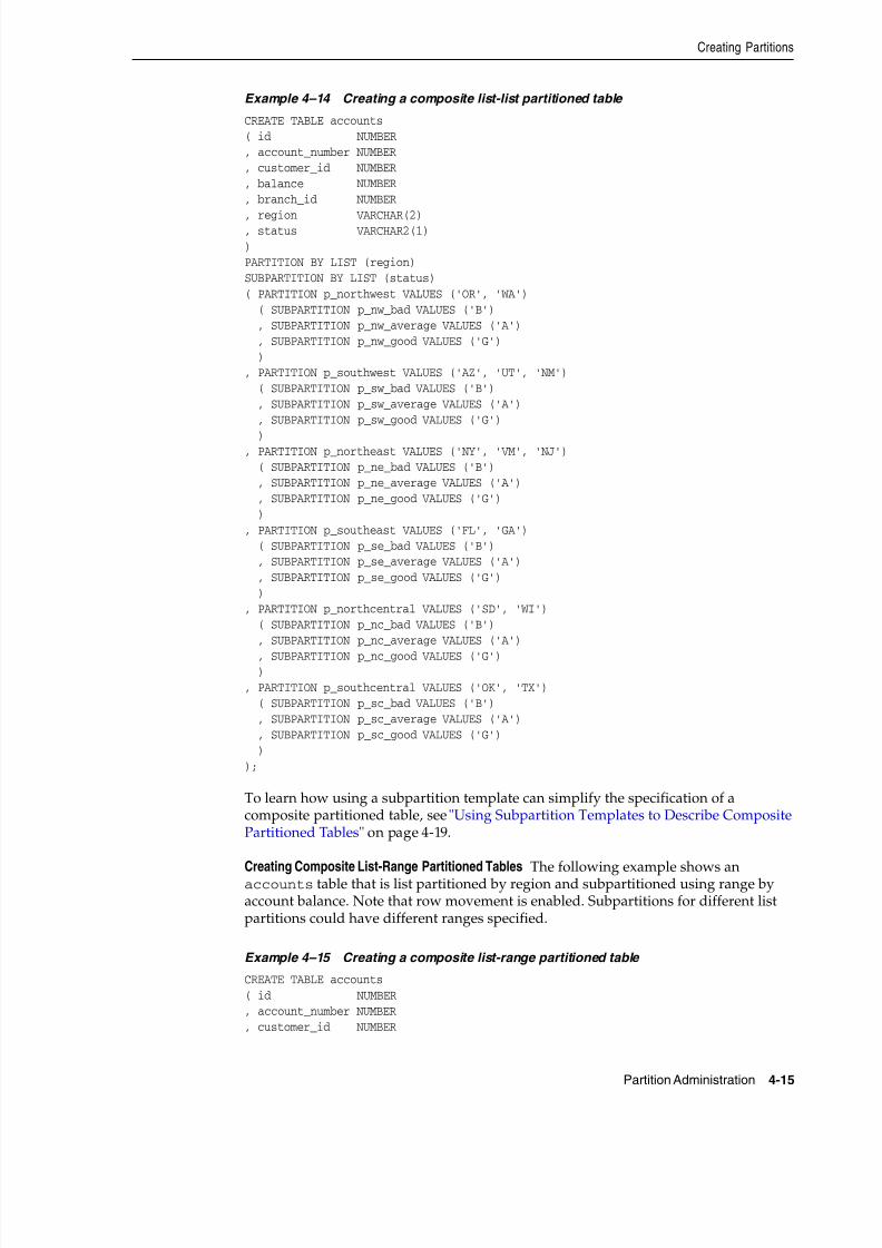
8/16/2019 Oracle Database VLDB and Partitioning Guide
http://slidepdf.com/reader/full/oracle-database-vldb-and-partitioning-guide 93/304
Creating Partitions
Partition Administration 4-15
Example 4–14 Creating a composite list-list partitioned table
CREATE TABLE accounts( id NUMBER, account_number NUMBER, customer_id NUMBER, balance NUMBER, branch_id NUMBER
, region VARCHAR(2), status VARCHAR2(1))PARTITION BY LIST (region)SUBPARTITION BY LIST (status)( PARTITION p_northwest VALUES ('OR', 'WA') ( SUBPARTITION p_nw_bad VALUES ('B') , SUBPARTITION p_nw_average VALUES ('A') , SUBPARTITION p_nw_good VALUES ('G') ), PARTITION p_southwest VALUES ('AZ', 'UT', 'NM') ( SUBPARTITION p_sw_bad VALUES ('B') , SUBPARTITION p_sw_average VALUES ('A') , SUBPARTITION p_sw_good VALUES ('G')
), PARTITION p_northeast VALUES ('NY', 'VM', 'NJ') ( SUBPARTITION p_ne_bad VALUES ('B') , SUBPARTITION p_ne_average VALUES ('A') , SUBPARTITION p_ne_good VALUES ('G') ), PARTITION p_southeast VALUES ('FL', 'GA') ( SUBPARTITION p_se_bad VALUES ('B') , SUBPARTITION p_se_average VALUES ('A') , SUBPARTITION p_se_good VALUES ('G') ), PARTITION p_northcentral VALUES ('SD', 'WI') ( SUBPARTITION p_nc_bad VALUES ('B') , SUBPARTITION p_nc_average VALUES ('A')
, SUBPARTITION p_nc_good VALUES ('G') ), PARTITION p_southcentral VALUES ('OK', 'TX') ( SUBPARTITION p_sc_bad VALUES ('B') , SUBPARTITION p_sc_average VALUES ('A') , SUBPARTITION p_sc_good VALUES ('G') ));
To learn how using a subpartition template can simplify the specification of acomposite partitioned table, see "Using Subpartition Templates to Describe CompositePartitioned Tables" on page 4-19.
Creating Composite List-Range Partitioned TablesThe following example shows anaccounts table that is list partitioned by region and subpartitioned using range by
account balance. Note that row movement is enabled. Subpartitions for different listpartitions could have different ranges specified.
Example 4–15 Creating a composite list-range partitioned table
CREATE TABLE accounts( id NUMBER, account_number NUMBER, customer_id NUMBER
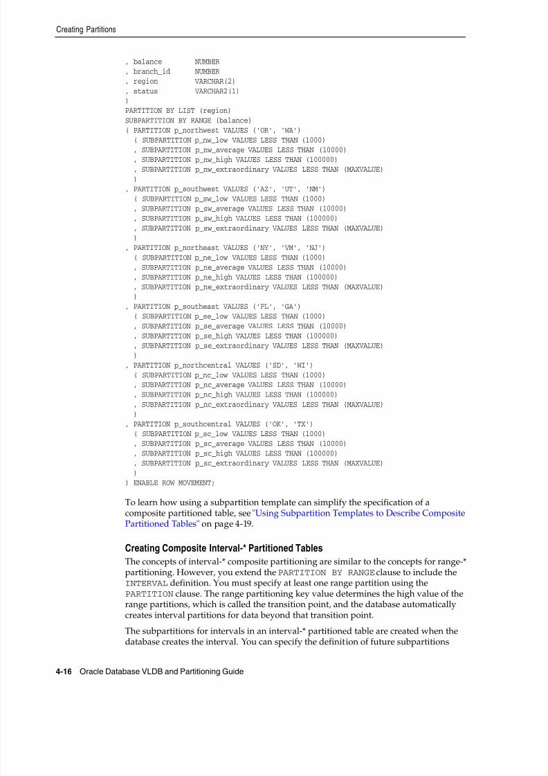
8/16/2019 Oracle Database VLDB and Partitioning Guide
http://slidepdf.com/reader/full/oracle-database-vldb-and-partitioning-guide 94/304
Creating Partitions
4-16 Oracle Database VLDB and Partitioning Guide
, balance NUMBER, branch_id NUMBER, region VARCHAR(2), status VARCHAR2(1))PARTITION BY LIST (region)SUBPARTITION BY RANGE (balance)( PARTITION p_northwest VALUES ('OR', 'WA') ( SUBPARTITION p_nw_low VALUES LESS THAN (1000) , SUBPARTITION p_nw_average VALUES LESS THAN (10000) , SUBPARTITION p_nw_high VALUES LESS THAN (100000) , SUBPARTITION p_nw_extraordinary VALUES LESS THAN (MAXVALUE) ), PARTITION p_southwest VALUES ('AZ', 'UT', 'NM') ( SUBPARTITION p_sw_low VALUES LESS THAN (1000) , SUBPARTITION p_sw_average VALUES LESS THAN (10000) , SUBPARTITION p_sw_high VALUES LESS THAN (100000) , SUBPARTITION p_sw_extraordinary VALUES LESS THAN (MAXVALUE) ), PARTITION p_northeast VALUES ('NY', 'VM', 'NJ') ( SUBPARTITION p_ne_low VALUES LESS THAN (1000) , SUBPARTITION p_ne_average VALUES LESS THAN (10000) , SUBPARTITION p_ne_high VALUES LESS THAN (100000) , SUBPARTITION p_ne_extraordinary VALUES LESS THAN (MAXVALUE) ), PARTITION p_southeast VALUES ('FL', 'GA') ( SUBPARTITION p_se_low VALUES LESS THAN (1000) , SUBPARTITION p_se_average VALUES LESS THAN (10000) , SUBPARTITION p_se_high VALUES LESS THAN (100000) , SUBPARTITION p_se_extraordinary VALUES LESS THAN (MAXVALUE) ), PARTITION p_northcentral VALUES ('SD', 'WI') ( SUBPARTITION p_nc_low VALUES LESS THAN (1000) , SUBPARTITION p_nc_average VALUES LESS THAN (10000) , SUBPARTITION p_nc_high VALUES LESS THAN (100000)
, SUBPARTITION p_nc_extraordinary VALUES LESS THAN (MAXVALUE) ), PARTITION p_southcentral VALUES ('OK', 'TX') ( SUBPARTITION p_sc_low VALUES LESS THAN (1000) , SUBPARTITION p_sc_average VALUES LESS THAN (10000) , SUBPARTITION p_sc_high VALUES LESS THAN (100000) , SUBPARTITION p_sc_extraordinary VALUES LESS THAN (MAXVALUE) )) ENABLE ROW MOVEMENT;
To learn how using a subpartition template can simplify the specification of acomposite partitioned table, see "Using Subpartition Templates to Describe CompositePartitioned Tables" on page 4-19.
Creating Composite Interval-* Partitioned TablesThe concepts of interval-* composite partitioning are similar to the concepts for range-*partitioning. However, you extend the PARTITION BY RANGE clause to include theINTERVAL definition. You must specify at least one range partition using thePARTITION clause. The range partitioning key value determines the high value of therange partitions, which is called the transition point, and the database automaticallycreates interval partitions for data beyond that transition point.
The subpartitions for intervals in an interval-* partitioned table are created when thedatabase creates the interval. You can specify the definition of future subpartitions
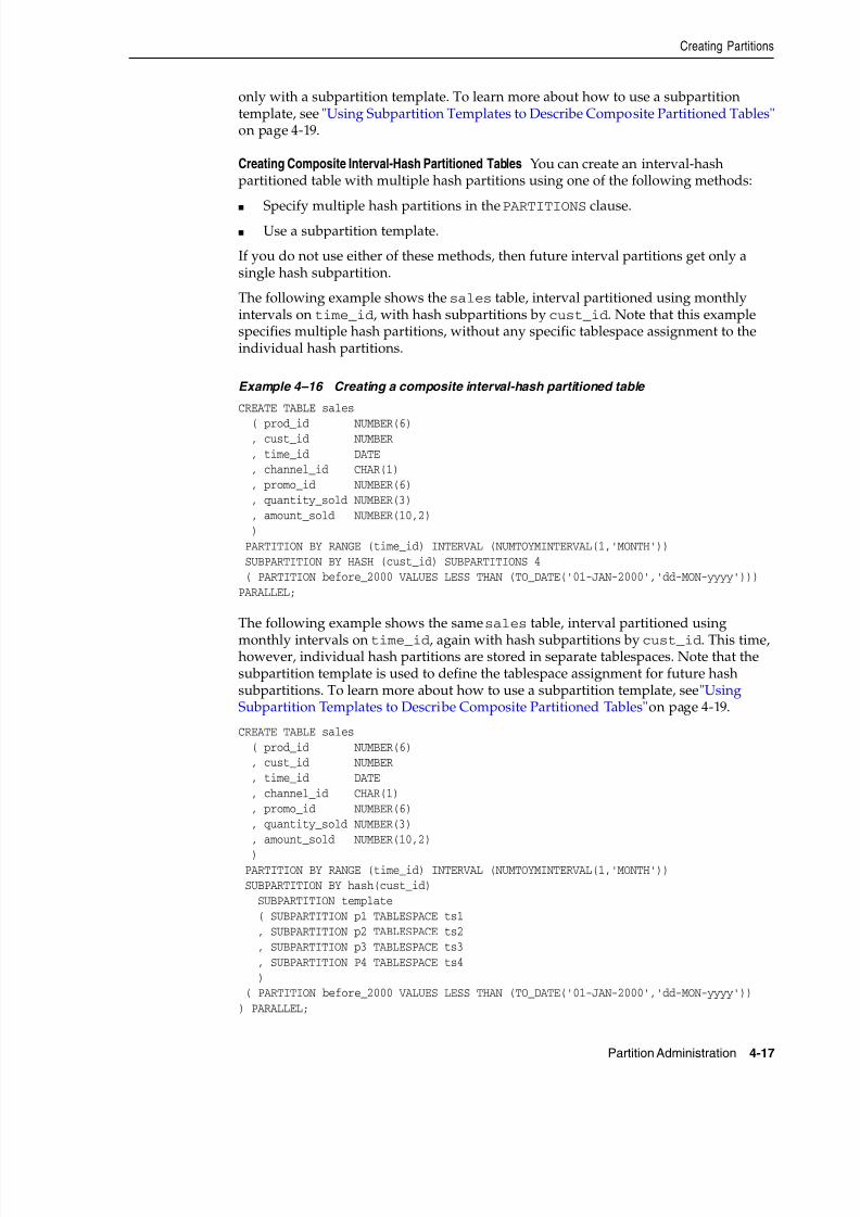
8/16/2019 Oracle Database VLDB and Partitioning Guide
http://slidepdf.com/reader/full/oracle-database-vldb-and-partitioning-guide 95/304
Creating Partitions
Partition Administration 4-17
only with a subpartition template. To learn more about how to use a subpartitiontemplate, see "Using Subpartition Templates to Describe Composite Partitioned Tables" on page 4-19.
Creating Composite Interval-Hash Partitioned Tables You can create an interval-hashpartitioned table with multiple hash partitions using one of the following methods:
■
Specify multiple hash partitions in the PARTITIONS clause.■ Use a subpartition template.
If you do not use either of these methods, then future interval partitions get only asingle hash subpartition.
The following example shows the sales table, interval partitioned using monthlyintervals on time_id, with hash subpartitions by cust_id. Note that this examplespecifies multiple hash partitions, without any specific tablespace assignment to theindividual hash partitions.
Example 4–16 Creating a composite interval-hash partitioned table
CREATE TABLE sales
( prod_id NUMBER(6) , cust_id NUMBER , time_id DATE , channel_id CHAR(1) , promo_id NUMBER(6) , quantity_sold NUMBER(3) , amount_sold NUMBER(10,2) ) PARTITION BY RANGE (time_id) INTERVAL (NUMTOYMINTERVAL(1,'MONTH')) SUBPARTITION BY HASH (cust_id) SUBPARTITIONS 4 ( PARTITION before_2000 VALUES LESS THAN (TO_DATE('01-JAN-2000','dd-MON-yyyy')))PARALLEL;
The following example shows the same sales table, interval partitioned using
monthly intervals on time_id, again with hash subpartitions by cust_id. This time,however, individual hash partitions are stored in separate tablespaces. Note that thesubpartition template is used to define the tablespace assignment for future hashsubpartitions. To learn more about how to use a subpartition template, see "UsingSubpartition Templates to Describe Composite Partitioned Tables" on page 4-19.
CREATE TABLE sales ( prod_id NUMBER(6) , cust_id NUMBER , time_id DATE , channel_id CHAR(1) , promo_id NUMBER(6) , quantity_sold NUMBER(3) , amount_sold NUMBER(10,2)
) PARTITION BY RANGE (time_id) INTERVAL (NUMTOYMINTERVAL(1,'MONTH')) SUBPARTITION BY hash(cust_id) SUBPARTITION template ( SUBPARTITION p1 TABLESPACE ts1 , SUBPARTITION p2 TABLESPACE ts2 , SUBPARTITION p3 TABLESPACE ts3 , SUBPARTITION P4 TABLESPACE ts4 ) ( PARTITION before_2000 VALUES LESS THAN (TO_DATE('01-JAN-2000','dd-MON-yyyy'))) PARALLEL;

8/16/2019 Oracle Database VLDB and Partitioning Guide
http://slidepdf.com/reader/full/oracle-database-vldb-and-partitioning-guide 96/304
Creating Partitions
4-18 Oracle Database VLDB and Partitioning Guide
Creating Composite Interval-List Partitioned Tables The only way to define list subpartitionsfor future interval partitions is with the subpartition template. If you do not use thesubpartitioning template, then the only subpartition that are created for every intervalpartition is a DEFAULT subpartition. To learn more about how to use a subpartitiontemplate, see "Using Subpartition Templates to Describe Composite Partitioned Tables"
on page 4-19.
The following example shows the sales table, interval partitioned using dailyintervals on time_id, with list subpartitions by channel_id.
Example 4–17 Creating a composite interval-list partitioned table
CREATE TABLE sales ( prod_id NUMBER(6) , cust_id NUMBER , time_id DATE , channel_id CHAR(1) , promo_id NUMBER(6) , quantity_sold NUMBER(3)
, amount_sold NUMBER(10,2) ) PARTITION BY RANGE (time_id) INTERVAL (NUMTODSINTERVAL(1,'DAY')) SUBPARTITION BY LIST (channel_id) SUBPARTITION TEMPLATE ( SUBPARTITION p_catalog VALUES ('C') , SUBPARTITION p_internet VALUES ('I') , SUBPARTITION p_partners VALUES ('P') , SUBPARTITION p_direct_sales VALUES ('S') , SUBPARTITION p_tele_sales VALUES ('T') ) ( PARTITION before_2000 VALUES LESS THAN (TO_DATE('01-JAN-2000','dd-MON-yyyy')))PARALLEL;
Creating Composite Interval-Range Partitioned Tables The only way to define rangesubpartitions for future interval partitions is with the subpartition template. If you donot use the subpartition template, then the only subpartition that is created for everyinterval partition is a range subpartition with the MAXVALUE upper boundary. To learnmore about how to use a subpartition template, see "Using Subpartition Templates toDescribe Composite Partitioned Tables" on page 4-19.
The following example shows the sales table, interval partitioned using dailyintervals on time_id, with range subpartitions by amount_sold.
Example 4–18 Creating a composite interval-range partitioned table
CREATE TABLE sales
( prod_id NUMBER(6) , cust_id NUMBER , time_id DATE , channel_id CHAR(1) , promo_id NUMBER(6) , quantity_sold NUMBER(3) , amount_sold NUMBER(10,2) ) PARTITION BY RANGE (time_id) INTERVAL (NUMTODSINTERVAL(1,'DAY'))SUBPARTITION BY RANGE(amount_sold) SUBPARTITION TEMPLATE
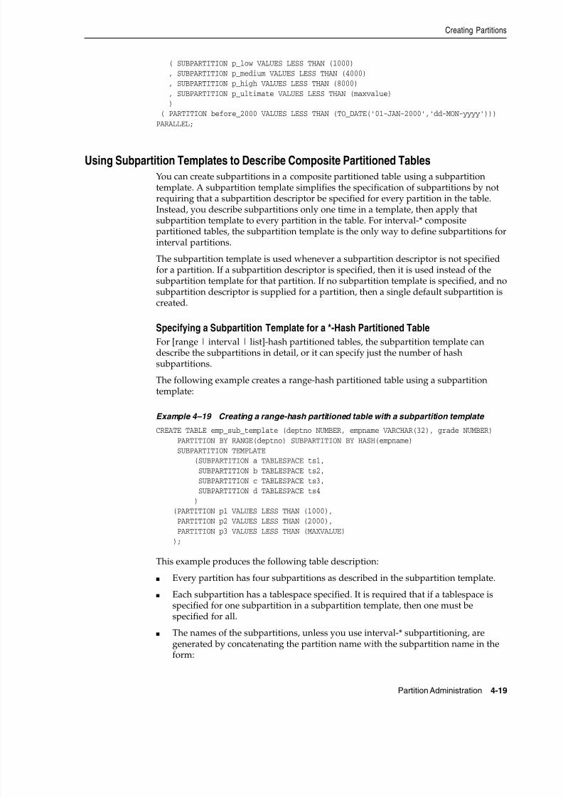
8/16/2019 Oracle Database VLDB and Partitioning Guide
http://slidepdf.com/reader/full/oracle-database-vldb-and-partitioning-guide 97/304
Creating Partitions
Partition Administration 4-19
( SUBPARTITION p_low VALUES LESS THAN (1000) , SUBPARTITION p_medium VALUES LESS THAN (4000) , SUBPARTITION p_high VALUES LESS THAN (8000) , SUBPARTITION p_ultimate VALUES LESS THAN (maxvalue) ) ( PARTITION before_2000 VALUES LESS THAN (TO_DATE('01-JAN-2000','dd-MON-yyyy')))PARALLEL;
Using Subpartition Templates to Describe Composite Partitioned TablesYou can create subpartitions in a composite partitioned table using a subpartitiontemplate. A subpartition template simplifies the specification of subpartitions by notrequiring that a subpartition descriptor be specified for every partition in the table.Instead, you describe subpartitions only one time in a template, then apply thatsubpartition template to every partition in the table. For interval-* compositepartitioned tables, the subpartition template is the only way to define subpartitions forinterval partitions.
The subpartition template is used whenever a subpartition descriptor is not specifiedfor a partition. If a subpartition descriptor is specified, then it is used instead of the
subpartition template for that partition. If no subpartition template is specified, and nosubpartition descriptor is supplied for a partition, then a single default subpartition iscreated.
Specifying a Subpartition Template for a *-Hash Partitioned Table
For [range | interval | list]-hash partitioned tables, the subpartition template candescribe the subpartitions in detail, or it can specify just the number of hashsubpartitions.
The following example creates a range-hash partitioned table using a subpartitiontemplate:
Example 4–19 Creating a range-hash partitioned table with a subpartition template CREATE TABLE emp_sub_template (deptno NUMBER, empname VARCHAR(32), grade NUMBER) PARTITION BY RANGE(deptno) SUBPARTITION BY HASH(empname) SUBPARTITION TEMPLATE (SUBPARTITION a TABLESPACE ts1, SUBPARTITION b TABLESPACE ts2, SUBPARTITION c TABLESPACE ts3, SUBPARTITION d TABLESPACE ts4 ) (PARTITION p1 VALUES LESS THAN (1000), PARTITION p2 VALUES LESS THAN (2000), PARTITION p3 VALUES LESS THAN (MAXVALUE) );
This example produces the following table description:
■ Every partition has four subpartitions as described in the subpartition template.
■ Each subpartition has a tablespace specified. It is required that if a tablespace isspecified for one subpartition in a subpartition template, then one must bespecified for all.
■ The names of the subpartitions, unless you use interval-* subpartitioning, aregenerated by concatenating the partition name with the subpartition name in theform:
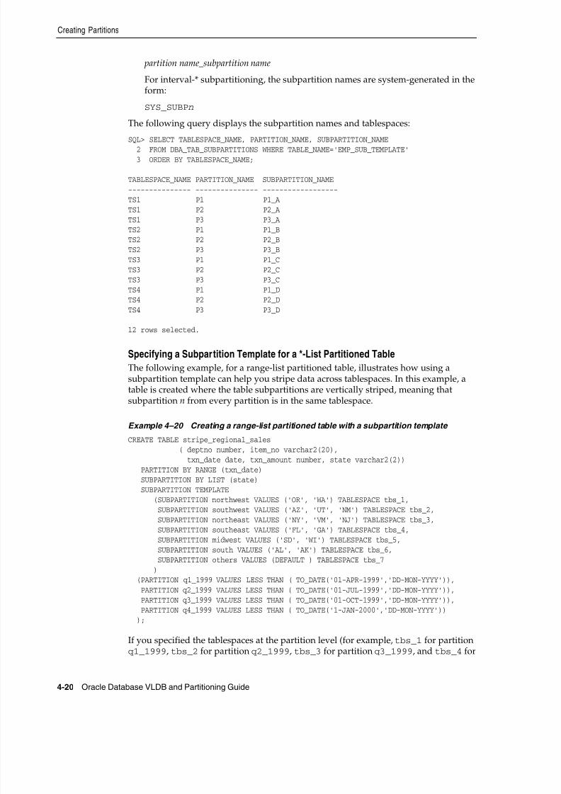
8/16/2019 Oracle Database VLDB and Partitioning Guide
http://slidepdf.com/reader/full/oracle-database-vldb-and-partitioning-guide 98/304
Creating Partitions
4-20 Oracle Database VLDB and Partitioning Guide
partition name_subpartition name
For interval-* subpartitioning, the subpartition names are system-generated in theform:
SYS_SUBPn
The following query displays the subpartition names and tablespaces:
SQL> SELECT TABLESPACE_NAME, PARTITION_NAME, SUBPARTITION_NAME 2 FROM DBA_TAB_SUBPARTITIONS WHERE TABLE_NAME='EMP_SUB_TEMPLATE' 3 ORDER BY TABLESPACE_NAME;
TABLESPACE_NAME PARTITION_NAME SUBPARTITION_NAME--------------- --------------- ------------------TS1 P1 P1_ATS1 P2 P2_ATS1 P3 P3_ATS2 P1 P1_BTS2 P2 P2_BTS2 P3 P3_BTS3 P1 P1_CTS3 P2 P2_C
TS3 P3 P3_CTS4 P1 P1_DTS4 P2 P2_DTS4 P3 P3_D
12 rows selected.
Specifying a Subpartition Template for a *-List Partitioned Table
The following example, for a range-list partitioned table, illustrates how using asubpartition template can help you stripe data across tablespaces. In this example, atable is created where the table subpartitions are vertically striped, meaning thatsubpartition n from every partition is in the same tablespace.
Example 4–20 Creating a range-list partitioned table with a subpartition template
CREATE TABLE stripe_regional_sales ( deptno number, item_no varchar2(20), txn_date date, txn_amount number, state varchar2(2)) PARTITION BY RANGE (txn_date) SUBPARTITION BY LIST (state) SUBPARTITION TEMPLATE
(SUBPARTITION northwest VALUES ('OR', 'WA') TABLESPACE tbs_1, SUBPARTITION southwest VALUES ('AZ', 'UT', 'NM') TABLESPACE tbs_2, SUBPARTITION northeast VALUES ('NY', 'VM', 'NJ') TABLESPACE tbs_3, SUBPARTITION southeast VALUES ('FL', 'GA') TABLESPACE tbs_4, SUBPARTITION midwest VALUES ('SD', 'WI') TABLESPACE tbs_5, SUBPARTITION south VALUES ('AL', 'AK') TABLESPACE tbs_6,
SUBPARTITION others VALUES (DEFAULT ) TABLESPACE tbs_7 ) (PARTITION q1_1999 VALUES LESS THAN ( TO_DATE('01-APR-1999','DD-MON-YYYY')), PARTITION q2_1999 VALUES LESS THAN ( TO_DATE('01-JUL-1999','DD-MON-YYYY')), PARTITION q3_1999 VALUES LESS THAN ( TO_DATE('01-OCT-1999','DD-MON-YYYY')), PARTITION q4_1999 VALUES LESS THAN ( TO_DATE('1-JAN-2000','DD-MON-YYYY')) );
If you specified the tablespaces at the partition level (for example, tbs_1 for partitionq1_1999, tbs_2 for partition q2_1999, tbs_3 for partition q3_1999, and tbs_4 for
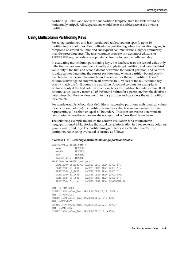
8/16/2019 Oracle Database VLDB and Partitioning Guide
http://slidepdf.com/reader/full/oracle-database-vldb-and-partitioning-guide 99/304
Creating Partitions
Partition Administration 4-21
partition q4_1999) and not in the subpartition template, then the table would behorizontally striped. All subpartitions would be in the tablespace of the owningpartition.
Using Multicolumn Partitioning KeysFor range-partitioned and hash-partitioned tables, you can specify up to 16
partitioning key columns. Use multicolumn partitioning when the partitioning key iscomposed of several columns and subsequent columns define a higher granularitythan the preceding ones. The most common scenario is a decomposed DATE orTIMESTAMP key, consisting of separated columns, for year, month, and day.
In evaluating multicolumn partitioning keys, the database uses the second value onlyif the first value cannot uniquely identify a single target partition, and uses the thirdvalue only if the first and second do not determine the correct partition, and so forth.A value cannot determine the correct partition only when a partition bound exactlymatches that value and the same bound is defined for the next partition. The nth column is investigated only when all previous (n-1) values of the multicolumn keyexactly match the (n-1) bounds of a partition. A second column, for example, isevaluated only if the first column exactly matches the partition boundary value. If all
column values exactly match all of the bound values for a partition, then the databasedetermines that the row does not fit in this partition and considers the next partitionfor a match.
For nondeterministic boundary definitions (successive partitions with identical valuesfor at least one column), the partition boundary value becomes an inclusive value,representing a "less than or equal to" boundary. This is in contrast to deterministic boundaries, where the values are always regarded as "less than" boundaries.
The following example illustrates the column evaluation for a multicolumnrange-partitioned table, storing the actual DATE information in three separate columns:year, month, and day. The partitioning granularity is a calendar quarter. Thepartitioned table being evaluated is created as follows:
Example 4–21 Creating a multicolumn range-partitioned table
CREATE TABLE sales_demo ( year NUMBER, month NUMBER,
day NUMBER, amount_sold NUMBER)PARTITION BY RANGE (year,month)(PARTITION before2001 VALUES LESS THAN (2001,1),
PARTITION q1_2001 VALUES LESS THAN (2001,4), PARTITION q2_2001 VALUES LESS THAN (2001,7), PARTITION q3_2001 VALUES LESS THAN (2001,10), PARTITION q4_2001 VALUES LESS THAN (2002,1), PARTITION future VALUES LESS THAN (MAXVALUE,0));
REM 12-DEC-2000INSERT INTO sales_demo VALUES(2000,12,12, 1000);REM 17-MAR-2001INSERT INTO sales_demo VALUES(2001,3,17, 2000);REM 1-NOV-2001INSERT INTO sales_demo VALUES(2001,11,1, 5000);REM 1-JAN-2002INSERT INTO sales_demo VALUES(2002,1,1, 4000);
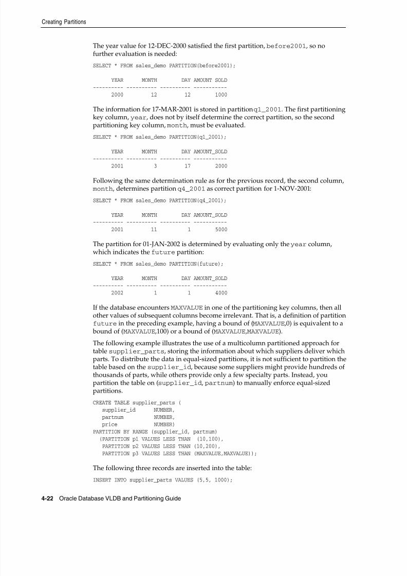
8/16/2019 Oracle Database VLDB and Partitioning Guide
http://slidepdf.com/reader/full/oracle-database-vldb-and-partitioning-guide 100/304
Creating Partitions
4-22 Oracle Database VLDB and Partitioning Guide
The year value for 12-DEC-2000 satisfied the first partition, before2001, so nofurther evaluation is needed:
SELECT * FROM sales_demo PARTITION(before2001);
YEAR MONTH DAY AMOUNT_SOLD---------- ---------- ---------- ----------- 2000 12 12 1000
The information for 17-MAR-2001 is stored in partition q1_2001. The first partitioningkey column, year, does not by itself determine the correct partition, so the secondpartitioning key column, month, must be evaluated.
SELECT * FROM sales_demo PARTITION(q1_2001);
YEAR MONTH DAY AMOUNT_SOLD---------- ---------- ---------- ----------- 2001 3 17 2000
Following the same determination rule as for the previous record, the second column, month, determines partition q4_2001 as correct partition for 1-NOV-2001:
SELECT * FROM sales_demo PARTITION(q4_2001);
YEAR MONTH DAY AMOUNT_SOLD---------- ---------- ---------- ----------- 2001 11 1 5000
The partition for 01-JAN-2002 is determined by evaluating only the year column,which indicates the future partition:
SELECT * FROM sales_demo PARTITION(future);
YEAR MONTH DAY AMOUNT_SOLD---------- ---------- ---------- ----------- 2002 1 1 4000
If the database encounters MAXVALUE in one of the partitioning key columns, then allother values of subsequent columns become irrelevant. That is, a definition of partitionfuture in the preceding example, having a bound of (MAXVALUE,0) is equivalent to a bound of (MAXVALUE,100) or a bound of (MAXVALUE,MAXVALUE).
The following example illustrates the use of a multicolumn partitioned approach fortable supplier_parts, storing the information about which suppliers deliver whichparts. To distribute the data in equal-sized partitions, it is not sufficient to partition thetable based on the supplier_id, because some suppliers might provide hundreds ofthousands of parts, while others provide only a few specialty parts. Instead, youpartition the table on (supplier_id, partnum ) to manually enforce equal-sizedpartitions.
CREATE TABLE supplier_parts ( supplier_id NUMBER,
partnum NUMBER, price NUMBER)PARTITION BY RANGE (supplier_id, partnum) (PARTITION p1 VALUES LESS THAN (10,100), PARTITION p2 VALUES LESS THAN (10,200), PARTITION p3 VALUES LESS THAN (MAXVALUE,MAXVALUE));
The following three records are inserted into the table:
INSERT INTO supplier_parts VALUES (5,5, 1000);

8/16/2019 Oracle Database VLDB and Partitioning Guide
http://slidepdf.com/reader/full/oracle-database-vldb-and-partitioning-guide 101/304
Creating Partitions
Partition Administration 4-23
INSERT INTO supplier_parts VALUES (5,150, 1000);INSERT INTO supplier_parts VALUES (10,100, 1000);
The first two records are inserted into partition p1, uniquely identified by supplier_id. However, the third record is inserted into partition p2; it matches all range boundary values of partition p1 exactly and the database therefore considers thefollowing partition for a match. The value of partnum satisfies the criteria < 200, so it
is inserted into partition p2.SELECT * FROM supplier_parts PARTITION (p1);
SUPPLIER_ID PARTNUM PRICE----------- ---------- ---------- 5 5 1000 5 150 1000
SELECT * FROM supplier_parts PARTITION (p2);
SUPPLIER_ID PARTNUM PRICE----------- ---------- ---------- 10 100 1000
Every row with supplier_id < 10 is stored in partition p1, regardless of thepartnum value. The column partnum is evaluated only if supplier_id =10, and thecorresponding rows is inserted into partition p1, p2, or even into p3 when partnum >=200. To achieve equal-sized partitions for ranges of supplier_parts, you couldchoose a composite range-hash partitioned table, range partitioned by supplier_id,hash subpartitioned by partnum .
Defining the partition boundaries for multicolumn partitioned tables must obey somerules. For example, consider a table that is range partitioned on three columns a, b,and c. The individual partitions have range values represented as follows:
P0(a0, b0, c0)P1(a1, b1, c1)P2(a2, b2, c2)...Pn(an, bn, cn)
The range values you provide for each partition must follow these rules:
■ a0 must be less than or equal to a1, and a1 must be less than or equal to a2, andso on.
■ If a0=a1, then b0 must be less than or equal to b1. If a0 < a1, then b0 and b1 canhave any values. If a0=a1 and b0=b1, then c0 must be less than or equal to c1. Ifb0<b1, then c0 and c1 can have any values, and so on.
■ If a1=a2, then b1 must be less than or equal to b2. If a1<a2, then b1 and b2 canhave any values. If a1=a2 and b1=b2, then c1 must be less than or equal to c2. If
b1<b2, then c1 and c2 can have any values, and so on.
Using Virtual Column-Based PartitioningWith partitioning, a virtual column can be used as any regular column. All partitionmethods are supported when using virtual columns, including interval partitioningand all different combinations of composite partitioning. A virtual column used as thepartitioning column cannot use calls to a PL/SQL function.
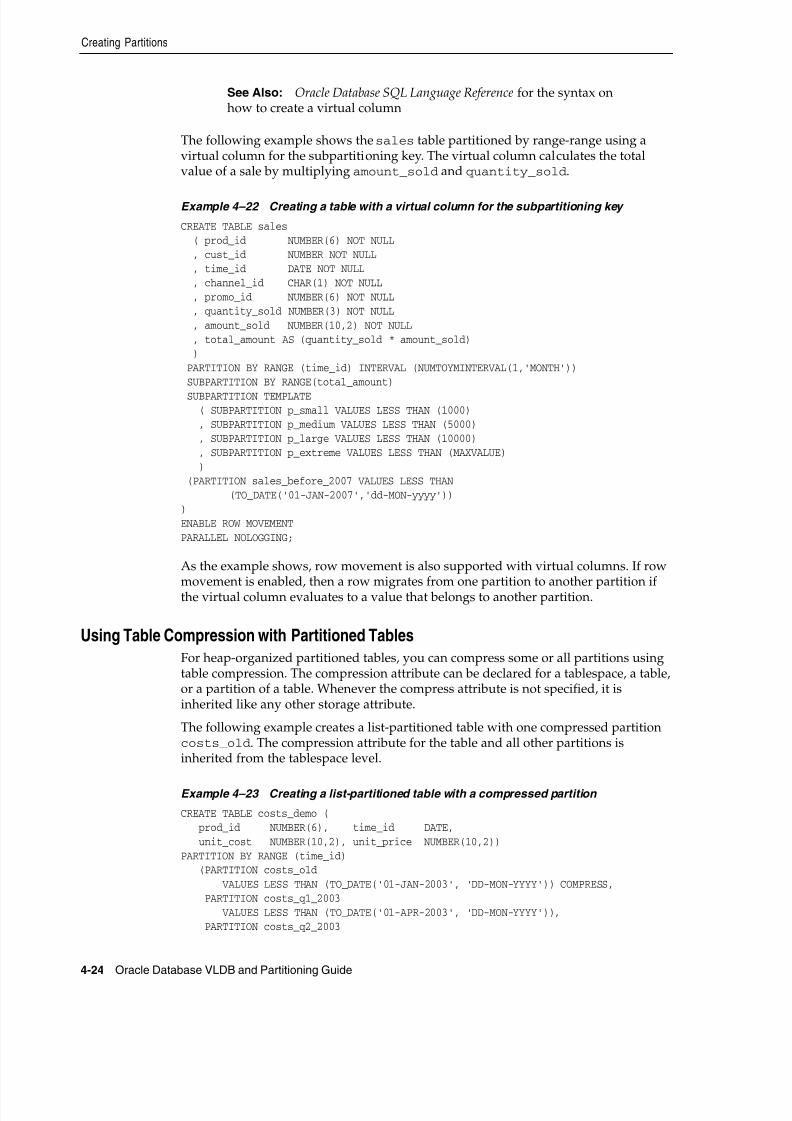
8/16/2019 Oracle Database VLDB and Partitioning Guide
http://slidepdf.com/reader/full/oracle-database-vldb-and-partitioning-guide 102/304
Creating Partitions
4-24 Oracle Database VLDB and Partitioning Guide
The following example shows the sales table partitioned by range-range using avirtual column for the subpartitioning key. The virtual column calculates the totalvalue of a sale by multiplying amount_sold and quantity_sold.
Example 4–22 Creating a table with a virtual column for the subpartitioning key
CREATE TABLE sales ( prod_id NUMBER(6) NOT NULL , cust_id NUMBER NOT NULL , time_id DATE NOT NULL , channel_id CHAR(1) NOT NULL , promo_id NUMBER(6) NOT NULL , quantity_sold NUMBER(3) NOT NULL , amount_sold NUMBER(10,2) NOT NULL , total_amount AS (quantity_sold * amount_sold) ) PARTITION BY RANGE (time_id) INTERVAL (NUMTOYMINTERVAL(1,'MONTH')) SUBPARTITION BY RANGE(total_amount)
SUBPARTITION TEMPLATE ( SUBPARTITION p_small VALUES LESS THAN (1000) , SUBPARTITION p_medium VALUES LESS THAN (5000) , SUBPARTITION p_large VALUES LESS THAN (10000) , SUBPARTITION p_extreme VALUES LESS THAN (MAXVALUE) ) (PARTITION sales_before_2007 VALUES LESS THAN (TO_DATE('01-JAN-2007','dd-MON-yyyy')))ENABLE ROW MOVEMENTPARALLEL NOLOGGING;
As the example shows, row movement is also supported with virtual columns. If rowmovement is enabled, then a row migrates from one partition to another partition ifthe virtual column evaluates to a value that belongs to another partition.
Using Table Compression with Partitioned TablesFor heap-organized partitioned tables, you can compress some or all partitions usingtable compression. The compression attribute can be declared for a tablespace, a table,or a partition of a table. Whenever the compress attribute is not specified, it isinherited like any other storage attribute.
The following example creates a list-partitioned table with one compressed partitioncosts_old. The compression attribute for the table and all other partitions isinherited from the tablespace level.
Example 4–23 Creating a list-partitioned table with a compressed partition
CREATE TABLE costs_demo ( prod_id NUMBER(6), time_id DATE,
unit_cost NUMBER(10,2), unit_price NUMBER(10,2))PARTITION BY RANGE (time_id) (PARTITION costs_old
VALUES LESS THAN (TO_DATE('01-JAN-2003', 'DD-MON-YYYY')) COMPRESS, PARTITION costs_q1_2003
VALUES LESS THAN (TO_DATE('01-APR-2003', 'DD-MON-YYYY')), PARTITION costs_q2_2003
See Also: Oracle Database SQL Language Reference for the syntax onhow to create a virtual column
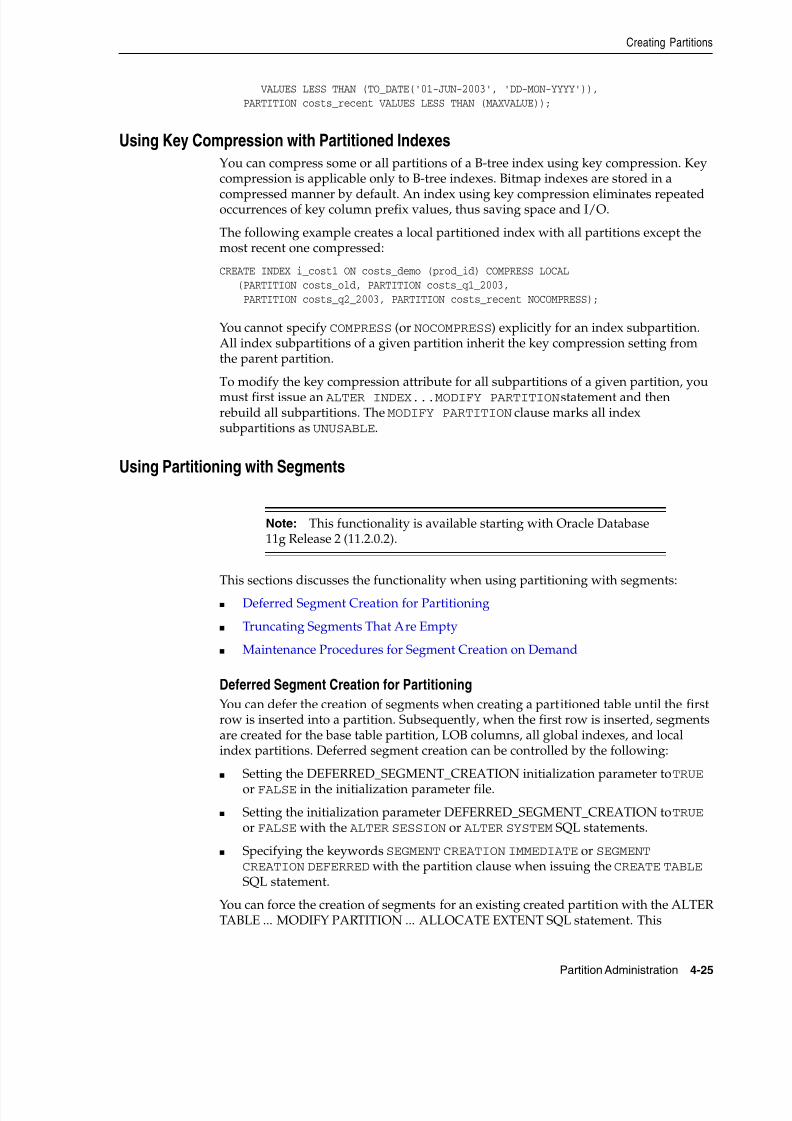
8/16/2019 Oracle Database VLDB and Partitioning Guide
http://slidepdf.com/reader/full/oracle-database-vldb-and-partitioning-guide 103/304
Creating Partitions
Partition Administration 4-25
VALUES LESS THAN (TO_DATE('01-JUN-2003', 'DD-MON-YYYY')), PARTITION costs_recent VALUES LESS THAN (MAXVALUE));
Using Key Compression with Partitioned IndexesYou can compress some or all partitions of a B-tree index using key compression. Keycompression is applicable only to B-tree indexes. Bitmap indexes are stored in a
compressed manner by default. An index using key compression eliminates repeatedoccurrences of key column prefix values, thus saving space and I/O.
The following example creates a local partitioned index with all partitions except themost recent one compressed:
CREATE INDEX i_cost1 ON costs_demo (prod_id) COMPRESS LOCAL (PARTITION costs_old, PARTITION costs_q1_2003,
PARTITION costs_q2_2003, PARTITION costs_recent NOCOMPRESS);
You cannot specify COMPRESS (or NOCOMPRESS) explicitly for an index subpartition.All index subpartitions of a given partition inherit the key compression setting fromthe parent partition.
To modify the key compression attribute for all subpartitions of a given partition, you
must first issue an ALTER INDEX...MODIFY PARTITION statement and thenrebuild all subpartitions. The MODIFY PARTITION clause marks all indexsubpartitions as UNUSABLE.
Using Partitioning with Segments
This sections discusses the functionality when using partitioning with segments:
■ Deferred Segment Creation for Partitioning
■ Truncating Segments That Are Empty
■ Maintenance Procedures for Segment Creation on Demand
Deferred Segment Creation for Partitioning
You can defer the creation of segments when creating a partitioned table until the firstrow is inserted into a partition. Subsequently, when the first row is inserted, segmentsare created for the base table partition, LOB columns, all global indexes, and localindex partitions. Deferred segment creation can be controlled by the following:
■ Setting the DEFERRED_SEGMENT_CREATION initialization parameter to TRUE
or FALSE in the initialization parameter file.
■ Setting the initialization parameter DEFERRED_SEGMENT_CREATION to TRUE or FALSE with the ALTER SESSION or ALTER SYSTEM SQL statements.
■ Specifying the keywords SEGMENT CREATION IMMEDIATE or SEGMENT CREATION DEFERRED with the partition clause when issuing the CREATE TABLE SQL statement.
You can force the creation of segments for an existing created partition with the ALTERTABLE ... MODIFY PARTITION ... ALLOCATE EXTENT SQL statement. This
Note: This functionality is available starting with Oracle Database11g Release 2 (11.2.0.2).

8/16/2019 Oracle Database VLDB and Partitioning Guide
http://slidepdf.com/reader/full/oracle-database-vldb-and-partitioning-guide 104/304
Creating Partitions
4-26 Oracle Database VLDB and Partitioning Guide
statement allocates one extent more than the initial number of extents specified duringthe CREATE TABLE.
Serializable transactions do not work with deferred segment creation. Inserting datainto an empty table with no segment created, or into a partition of an intervalpartitioned table that does not have a segment yet, causes an error.
Truncating Segments That Are Empty
You can drop empty segments in tables and table fragments with the DBMS_SPACE_
ADMIN.DROP_EMPTY_SEGMENTS procedure.In addition, if a partition or subpartition has a segment, then the truncate featuredrops the segment if the DROP ALL STORAGE clause is specified with the ALTER TABLE TRUNCATE PARTITION SQL statement.
Maintenance Procedures for Segment Creation on Demand
You can use the MATERIALIZE_DEFERRED_SEGMENTS procedure in the DBMS_SPACE_ADMIN package to create segments for tables and dependent objects for tableswith the deferred segment property.
You can also force the creation of segments for an existing created table and tablefragment with the DBMS_SPACE_ADMIN.MATERIALIZE_DEFERRED_SEGMENTS procedure. The MATERIALIZE_DEFERRED_SEGMENTS procedure differs from theALTER TABLE ... MODIFY PARTITION ... ALLOCATE EXTENT SQL statement because it does not allocate one additional extent for the table or table fragment.
Creating Partitioned Index-Organized TablesFor index-organized tables, you can use the range, list, or hash partitioning method.The semantics for creating partitioned index-organized tables is similar to that forregular tables with these differences:
■ When you create the table, you specify the ORGANIZATION INDEX clause, andINCLUDING and OVERFLOW clauses as necessary.
See Also:
■ Oracle Database Reference for more information about theDEFERRED_SEGMENT_CREATION initialization parameter
■ Oracle Database SQL Language Reference for more information aboutthe ALTER SESSION and ALTER SYSTEM SQL statements
■ Oracle Database SQL Language Reference for more information aboutthe keywords SEGMENT CREATION IMMEDIATE and SEGMENT CREATION DEFERRED of the CREATE TABLE SQL statement
See Also:
■ Oracle Database PL/SQL Packages and Types Reference for moreinformation about the DBMS_SPACE_ADMIN package
■ Oracle Database SQL Language Reference for more information aboutthe DROP ALL STORAGE clause of ALTER TABLE
See Also:
■ Oracle Database PL/SQL Packages and Types Reference for more
information about the DBMS_SPACE_ADMIN package

8/16/2019 Oracle Database VLDB and Partitioning Guide
http://slidepdf.com/reader/full/oracle-database-vldb-and-partitioning-guide 105/304
Creating Partitions
Partition Administration 4-27
■ The PARTITION or PARTITIONS clauses can have OVERFLOW subclauses thatallow you to specify attributes of the overflow segments at the partition level.
Specifying an OVERFLOW clause results in the overflow data segments themselves being equipartitioned with the primary key index segments. Thus, for partitionedindex-organized tables with overflow, each partition has an index segment and anoverflow data segment.
For index-organized tables, the set of partitioning columns must be a subset of theprimary key columns. Because rows of an index-organized table are stored in theprimary key index for the table, the partitioning criterion affects the availability. Bychoosing the partitioning key to be a subset of the primary key, an insert operationmust only verify uniqueness of the primary key in a single partition, therebymaintaining partition independence.
Support for secondary indexes on index-organized tables is similar to the support forregular tables. Because of the logical nature of the secondary indexes, global indexeson index-organized tables remain usable for certain operations where they would bemarked UNUSABLE for regular tables. For more information, refer to "MaintainingPartitions" on page 4-31.
Creating Range-Partitioned Index-Organized Tables
You can partition index-organized tables, and their secondary indexes, by the rangemethod. In the following example, a range-partitioned index-organized table sales iscreated. The INCLUDING clause specifies that all columns after week_no are to bestored in an overflow segment. There is one overflow segment for each partition, allstored in the same tablespace (overflow_here). Optionally, OVERFLOWTABLESPACE could be specified at the individual partition level, in which case someor all of the overflow segments could have separate TABLESPACE attributes.
Example 4–24 Creating a range-partitioned index-organized table
CREATE TABLE sales(acct_no NUMBER(5),acct_name CHAR(30),amount_of_sale NUMBER(6),
week_no INTEGER, sale_details VARCHAR2(1000), PRIMARY KEY (acct_no, acct_name, week_no))
ORGANIZATION INDEXINCLUDING week_no
OVERFLOW TABLESPACE overflow_here PARTITION BY RANGE (week_no) (PARTITION VALUES LESS THAN (5)
TABLESPACE ts1, PARTITION VALUES LESS THAN (9)
TABLESPACE ts2 OVERFLOW TABLESPACE overflow_ts2, ... PARTITION VALUES LESS THAN (MAXVALUE)
TABLESPACE ts13);
See Also:■ Oracle Database Administrator's Guide for more information about
managing index-organized tables
■ Oracle Database Concepts for more information aboutindex-organized tables

8/16/2019 Oracle Database VLDB and Partitioning Guide
http://slidepdf.com/reader/full/oracle-database-vldb-and-partitioning-guide 106/304
Creating Partitions
4-28 Oracle Database VLDB and Partitioning Guide
Creating Hash-Partitioned Index-Organized Tables
Another option for partitioning index-organized tables is to use the hash method. Inthe following example, the sales index-organized table is partitioned by the hashmethod.
Example 4–25 Creating a hash-partitioned index-organized table
CREATE TABLE sales(acct_no NUMBER(5),acct_name CHAR(30),amount_of_sale NUMBER(6),
week_no INTEGER, sale_details VARCHAR2(1000), PRIMARY KEY (acct_no, acct_name, week_no))
ORGANIZATION INDEXINCLUDING week_no
OVERFLOW PARTITION BY HASH (week_no) PARTITIONS 16 STORE IN (ts1, ts2, ts3, ts4) OVERFLOW STORE IN (ts3, ts6, ts9);
Creating List-Partitioned Index-Organized Tables
The other option for partitioning index-organized tables is to use the list method. Inthe following example, the sales index-organized table is partitioned by the list
method. This example uses the example tablespace, which is part of the sampleschemas in your seed database. Normally you would specify different tablespacestorage for different partitions.
Example 4–26 Creating a list-partitioned index-organized table
CREATE TABLE sales(acct_no NUMBER(5),acct_name CHAR(30),amount_of_sale NUMBER(6),
week_no INTEGER, sale_details VARCHAR2(1000), PRIMARY KEY (acct_no, acct_name, week_no))
ORGANIZATION INDEXINCLUDING week_no
OVERFLOW TABLESPACE example PARTITION BY LIST (week_no) (PARTITION VALUES (1, 2, 3, 4)
TABLESPACE example, PARTITION VALUES (5, 6, 7, 8)
TABLESPACE example OVERFLOW TABLESPACE example, PARTITION VALUES (DEFAULT)
TABLESPACE example);
Note: A well-designed hash function is intended to distribute rowsin a well-balanced fashion among the partitions. Therefore, updatingthe primary key column(s) of a row is very likely to move that row toa different partition. Oracle recommends that you explicitly specifythe ENABLE ROW MOVEMENT clause when creating a hash-partitionedindex-organized table with a changeable partitioning key. The defaultis that ENABLE ROW MOVEMENT is disabled.
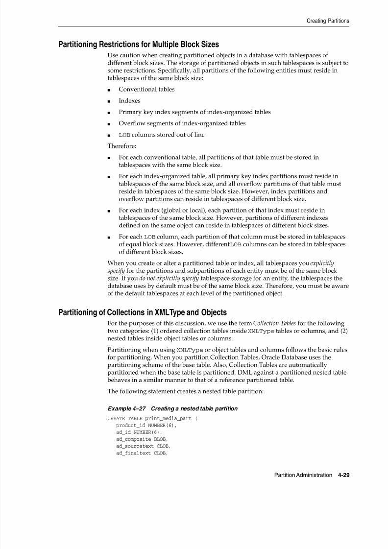
8/16/2019 Oracle Database VLDB and Partitioning Guide
http://slidepdf.com/reader/full/oracle-database-vldb-and-partitioning-guide 107/304

8/16/2019 Oracle Database VLDB and Partitioning Guide
http://slidepdf.com/reader/full/oracle-database-vldb-and-partitioning-guide 108/304
Creating Partitions
4-30 Oracle Database VLDB and Partitioning Guide
ad_fltextn NCLOB, ad_textdocs_ntab TEXTDOC_TAB, ad_photo BLOB, ad_graphic BFILE, ad_header ADHEADER_TYP)NESTED TABLE ad_textdocs_ntab STORE AS textdoc_ntPARTITION BY RANGE (product_id) (PARTITION p1 VALUES LESS THAN (100), PARTITION p2 VALUES LESS THAN (200));
For an example of issuing a query against a partitioned nested table and using theEXPLAIN PLAN to improve performance, see "Collection Tables" on page 3-10.
Note that Oracle Database provides a LOCAL keyword to equipartition a CollectionTable with a partitioned base table. This is the default behavior in this release. Thedefault in earlier releases was not to equipartition the Collection Table with thepartitioned base table. Now you must specify the GLOBAL keyword to store anunpartitioned Collection Table with a partitioned base table. See Oracle Database SQLLanguage Reference for more information. Also, to convert your existing nonpartitionedcollection tables to partitioned, use online redefinition, as illustrated in "RedefiningPartitions Online" on page 4-60.
Out-of-line (OOL) table partitioning is supported. However, you cannot create twotables of the same XML schema that has out-of-line tables. This means that exchangepartitioning cannot be performed for schemas with OOL tables because it is notpossible to have two tables of the same schema.
Performing PMOs on Partitions that Contain Collection Tables
Whether a partition contains Collection Tables or not does not significantly affect yourability to perform partition maintenance operations (PMOs). Usually, maintenanceoperations on Collection Tables are carried out on the base table. The followingexample illustrates a typical ADD PARTITION operation based on the preceding nestedtable partition:
ALTER TABLE print_media_partADD PARTITION p4 VALUES LESS THAN (400) LOB(ad_photo, ad_composite) STORE AS (TABLESPACE omf_ts1) LOB(ad_sourcetext, ad_finaltext) STORE AS (TABLESPACE omf_ts1) NESTED TABLE ad_textdocs_ntab STORE AS nt_p3;
The storage table for nested table storage column ad_textdocs_ntab is named nt_p3 and inherits all other attributes from the table-level defaults and then from thetablespace defaults.
You must directly invoke the following partition maintenance operations on thestorage table corresponding to the collection column:
■ modify partition
■ move partition
■ rename partition
■ modify the default attributes of a partition
See Also: Oracle Database SQL Language Reference for syntax andTable 4–1, " ALTER TABLE Maintenance Operations for TablePartitions" for a list of partition maintenance operations that can beperformed on partitioned tables and composite partitioned tables

8/16/2019 Oracle Database VLDB and Partitioning Guide
http://slidepdf.com/reader/full/oracle-database-vldb-and-partitioning-guide 109/304
Maintaining Partitions
Partition Administration 4-31
Maintaining PartitionsThis section describes how to perform partition and subpartition maintenanceoperations for both tables and indexes.
Table 4–1 lists partition maintenance operations that can be performed on partitionedtables and composite partitioned tables, and Table 4–2 lists subpartition maintenanceoperations that can be performed on composite partitioned tables. For each type ofpartitioning and subpartitioning, the specific clause of the ALTER TABLE statementthat is used to perform that maintenance operation is listed.
Table 4–1 ALTER TABLE Maintenance Operations for Table Partitions
MaintenanceOperation
Range
CompositeRange-*
Interval
CompositeInterval-* Hash
List
Composite List-* Reference
Adding Partitions ADD PARTITION ADD PARTITION ADD PARTITION ADD PARTITION N/A1
1 These operations cannot be performed on reference-partitioned tables. If performed on a parent table, then these operationscascade to all descendant tables.
Coalescing Partitions N/A N/A COALESCEPARTITION
N/A N/A1
Dropping Partitions DROPPARTITION
DROPPARTITION
N/A DROPPARTITION
N/A1
Exchanging Partitions EXCHANGEPARTITION
EXCHANGEPARTITION
EXCHANGEPARTITION
EXCHANGEPARTITION
EXCHANGEPARTITION
Merging Partitions MERGEPARTITIONS
MERGEPARTITIONS
N/A MERGEPARTITIONS
N/A1
Modifying DefaultAttributes
MODIFYDEFAULTATTRIBUTES
MODIFYDEFAULTATTRIBUTES
MODIFYDEFAULTATTRIBUTES
MODIFYDEFAULTATTRIBUTES
MODIFYDEFAULTATTRIBUTES
Modifying RealAttributes of Partitions
MODIFYPARTITION
MODIFYPARTITION
MODIFYPARTITION
MODIFYPARTITION
MODIFYPARTITION
Modifying ListPartitions: AddingValues
N/A N/A N/A MODIFYPARTITION ...ADD VALUES
N/A
Modifying List
Partitions: DroppingValues
N/A N/A N/A MODIFY
PARTITION ...DROP VALUES
N/A
Moving Partitions MOVESUBPARTITION
MOVESUBPARTITION
MOVEPARTITION
MOVESUBPARTITION
MOVEPARTITION
Renaming Partitions RENAMEPARTITION
RENAMEPARTITION
RENAMEPARTITION
RENAMEPARTITION
RENAMEPARTITION
Splitting Partitions SPLITPARTITION
SPLITPARTITION
N/A SPLITPARTITION
N/A1
Truncating Partitions TRUNCATEPARTITION
TRUNCATEPARTITION
TRUNCATEPARTITION
TRUNCATEPARTITION
TRUNCATEPARTITION
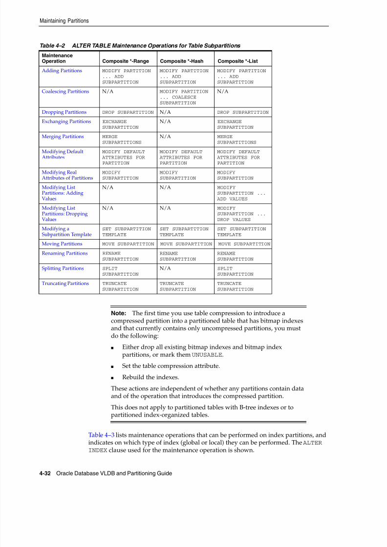
8/16/2019 Oracle Database VLDB and Partitioning Guide
http://slidepdf.com/reader/full/oracle-database-vldb-and-partitioning-guide 110/304
Maintaining Partitions
4-32 Oracle Database VLDB and Partitioning Guide
Table 4–3 lists maintenance operations that can be performed on index partitions, andindicates on which type of index (global or local) they can be performed. The ALTERINDEX clause used for the maintenance operation is shown.
Table 4–2 ALTER TABLE Maintenance Operations for Table Subpartitions
MaintenanceOperation Composite *-Range Composite *-Hash Composite *-List
Adding Partitions MODIFY PARTITION... ADDSUBPARTITION
MODIFY PARTITION... ADDSUBPARTITION
MODIFY PARTITION... ADDSUBPARTITION
Coalescing Partitions N/A MODIFY PARTITION
... COALESCESUBPARTITION
N/A
Dropping Partitions DROP SUBPARTITION N/A DROP SUBPARTITION
Exchanging Partitions EXCHANGESUBPARTITION
N/A EXCHANGESUBPARTITION
Merging Partitions MERGESUBPARTITIONS
N/A MERGESUBPARTITIONS
Modifying DefaultAttributes
MODIFY DEFAULTATTRIBUTES FORPARTITION
MODIFY DEFAULTATTRIBUTES FORPARTITION
MODIFY DEFAULTATTRIBUTES FORPARTITION
Modifying RealAttributes of Partitions
MODIFYSUBPARTITION
MODIFYSUBPARTITION
MODIFYSUBPARTITION
Modifying List
Partitions: AddingValues
N/A N/A MODIFY
SUBPARTITION ...ADD VALUES
Modifying ListPartitions: DroppingValues
N/A N/A MODIFYSUBPARTITION ...DROP VALUES
Modifying aSubpartition Template
SET SUBPARTITIONTEMPLATE
SET SUBPARTITIONTEMPLATE
SET SUBPARTITIONTEMPLATE
Moving Partitions MOVE SUBPARTITION MOVE SUBPARTITION MOVE SUBPARTITION
Renaming Partitions RENAMESUBPARTITION
RENAMESUBPARTITION
RENAMESUBPARTITION
Splitting Partitions SPLITSUBPARTITION
N/A SPLITSUBPARTITION
Truncating Partitions TRUNCATE
SUBPARTITION
TRUNCATE
SUBPARTITION
TRUNCATE
SUBPARTITION
Note: The first time you use table compression to introduce acompressed partition into a partitioned table that has bitmap indexesand that currently contains only uncompressed partitions, you mustdo the following:
■ Either drop all existing bitmap indexes and bitmap indexpartitions, or mark them UNUSABLE.
■ Set the table compression attribute.
■ Rebuild the indexes.
These actions are independent of whether any partitions contain dataand of the operation that introduces the compressed partition.
This does not apply to partitioned tables with B-tree indexes or topartitioned index-organized tables.
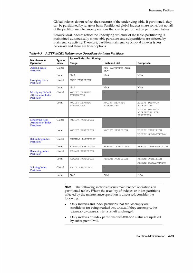
8/16/2019 Oracle Database VLDB and Partitioning Guide
http://slidepdf.com/reader/full/oracle-database-vldb-and-partitioning-guide 111/304
Maintaining Partitions
Partition Administration 4-33
Global indexes do not reflect the structure of the underlying table. If partitioned, theycan be partitioned by range or hash. Partitioned global indexes share some, but not all,of the partition maintenance operations that can be performed on partitioned tables.
Because local indexes reflect the underlying structure of the table, partitioning ismaintained automatically when table partitions and subpartitions are affected bymaintenance activity. Therefore, partition maintenance on local indexes is less
necessary and there are fewer options.
Table 4–3 ALTER INDEX Maintenance Operations for Index Partitions
MaintenanceOperation
Type ofIndex
Type of Index Partitioning
Range Hash and List Composite
Adding IndexPartitions
Global - ADD PARTITION (hashonly)
-
Local N/A N/A N/A
Dropping IndexPartitions
Global DROP PARTITION - -
Local N/A N/A N/A
Modifying Default
Attributes of IndexPartitions
Global MODIFY DEFAULT
ATTRIBUTES
- -
Local MODIFY DEFAULTATTRIBUTES
MODIFY DEFAULTATTRIBUTES
MODIFY DEFAULTATTRIBUTES
MODIFY DEFAULTATTRIBUTES FORPARTITION
Modifying RealAttributes of IndexPartitions
Global MODIFY PARTITION - -
Local MODIFY PARTITION MODIFY PARTITION MODIFY PARTITION
MODIFY SUBPARTITION
Rebuilding IndexPartitions
Global REBUILD PARTITION - -
Local REBUILD PARTITION REBUILD PARTITION REBUILD SUBPARTITION
Renaming IndexPartitions
Global RENAME PARTITION - -
Local RENAME PARTITION RENAME PARTITION RENAME PARTITION
RENAME SUBPARTITION
Splitting IndexPartitions
Global SPLIT PARTITION - -
Local N/A N/A N/A
Note: The following sections discuss maintenance operations on
partitioned tables. Where the usability of indexes or index partitionsaffected by the maintenance operation is discussed, consider thefollowing:
■ Only indexes and index partitions that are not empty arecandidates for being marked UNUSABLE. If they are empty, theUSABLE/UNUSABLE status is left unchanged.
■ Only indexes or index partitions with USABLE status are updated by subsequent DML.

8/16/2019 Oracle Database VLDB and Partitioning Guide
http://slidepdf.com/reader/full/oracle-database-vldb-and-partitioning-guide 112/304
8/16/2019 Oracle Database VLDB and Partitioning Guide
http://slidepdf.com/reader/full/oracle-database-vldb-and-partitioning-guide 113/304
Maintaining Partitions
Partition Administration 4-35
SKIP_UNUSABLE_INDEXES Initialization Parameter
SKIP_UNUSABLE_INDEXES is an initialization parameter with a default value ofTRUE. This setting disables error reporting of indexes and index partitions markedUNUSABLE. If you do not want the database to choose an alternative execution plan toavoid the unusable elements, then you should set this parameter to FALSE.
Considerations when Updating Indexes Automatically
The following implications are worth noting when you specify UPDATE INDEXES:
■ The partition DDL statement takes longer to execute, because indexes that werepreviously marked UNUSABLE are updated. However, you must compare thisincrease with the time it takes to execute DDL without updating indexes, and thenrebuild all indexes. A rule of thumb is that it is faster to update indexes if the sizeof the partition is less that 5% of the size of the table.
■ The DROP, TRUNCATE, and EXCHANGE operations are no longer fast operations.Again, you must compare the time it takes to do the DDL and then rebuild allindexes.
■ When you update a table with a global index:
– The index is updated in place. The updates to the index are logged, and redoand undo records are generated. In contrast, if you rebuild an entire globalindex, you can do so in NOLOGGING mode.
– Rebuilding the entire index manually creates a more efficient index, because itis more compact with better space utilization.
■ The UPDATE INDEXES clause is not supported for index-organized tables.However, the UPDATE GLOBAL INDEXES clause may be used with DROP PARTITION, TRUNCATE PARTITION, and EXCHANGE PARTITION operations tokeep the global indexes on index-organized tables usable. For the remainingoperations in the above list, global indexes on index-organized tables remainusable. In addition, local index partitions on index-organized tables remain usableafter a MOVE PARTITION operation.
Adding PartitionsThis section describes how to manually add new partitions to a partitioned table andexplains why partitions cannot be specifically added to most partitioned indexes.
Adding a Partition to a Range-Partitioned Table
Use the ALTER TABLE ... ADD PARTITION statement to add a new partition to the"high" end (the point after the last existing partition). To add a partition at the beginning or in the middle of a table, use the SPLIT PARTITION clause.
For example, consider the table, sales, which contains data for the current month inaddition to the previous 12 months. On January 1, 1999, you add a partition for January, which is stored in tablespace tsx.
ALTER TABLE sales ADD PARTITION jan99 VALUES LESS THAN ( '01-FEB-1999' ) TABLESPACE tsx;
Local and global indexes associated with the range-partitioned table remain usable.

8/16/2019 Oracle Database VLDB and Partitioning Guide
http://slidepdf.com/reader/full/oracle-database-vldb-and-partitioning-guide 114/304
Maintaining Partitions
4-36 Oracle Database VLDB and Partitioning Guide
Adding a Partition to a Hash-Partitioned Table
When you add a partition to a hash-partitioned table, the database populates the newpartition with rows rehashed from an existing partition (selected by the database) asdetermined by the hash function. Consequently, if the table contains data, then it maytake some time to add a hash partition.
The following statements show two ways of adding a hash partition to table
scubagear. Choosing the first statement adds a new hash partition whose partitionname is system generated, and which is placed in the default tablespace. The secondstatement also adds a new hash partition, but that partition is explicitly named p_named and is created in tablespace gear5.
ALTER TABLE scubagear ADD PARTITION;
ALTER TABLE scubagear ADD PARTITION p_named TABLESPACE gear5;
Indexes may be marked UNUSABLE as explained in the following table:
Adding a Partition to a List-Partitioned Table
The following statement illustrates how to add a new partition to a list-partitionedtable. In this example, physical attributes and NOLOGGING are specified for thepartition being added.
ALTER TABLE q1_sales_by_regionADD PARTITION q1_nonmainland VALUES ('HI', 'PR')
STORAGE (INITIAL 20K NEXT 20K) TABLESPACE tbs_3 NOLOGGING;
Any value in the set of literal values that describe the partition being added must notexist in any of the other partitions of the table.
You cannot add a partition to a list-partitioned table that has a default partition, butyou can split the default partition. By doing so, you effectively create a new partitiondefined by the values that you specify, and a second partition that remains the default
partition.
Local and global indexes associated with the list-partitioned table remain usable.
Adding a Partition to an Interval-Partitioned Table
You cannot explicitly add a partition to an interval-partitioned table unless you firstlock the partition, which triggers the creation of the partition. The databaseautomatically creates a partition for an interval when data for that interval is inserted.In general, you only must explicitly create interval partitions for a partition exchangeload scenario.
Table Type Index Behavior
Regular (Heap) Unless you specify UPDATE INDEXES as part of the ALTER TABLE statement:
■ The local indexes for the new partition, and for the existingpartition from which rows were redistributed, are markedUNUSABLE and must be rebuilt.
■ All global indexes, or all partitions of partitioned globalindexes, are marked UNUSABLE and must be rebuilt.
Index-organized ■ For local indexes, the behavior is identical to heap tables.
■ All global indexes remain usable.

8/16/2019 Oracle Database VLDB and Partitioning Guide
http://slidepdf.com/reader/full/oracle-database-vldb-and-partitioning-guide 115/304
Maintaining Partitions
Partition Administration 4-37
To change the interval for future partitions, use the SET INTERVAL clause of theALTER TABLE statement. This clause changes the interval for partitions beyond thecurrent highest boundary of all materialized interval partitions.
You also use the SET INTERVAL clause to migrate an existing range partitioned orrange-* composite partitioned table into an interval or interval-* partitioned table. Todisable the creation of future interval partitions, and effectively revert back to a
range-partitioned table, then use an empty value in the SET INTERVAL clause.Created interval partitions are transformed into range partitions with their currenthigh values.
To increase the interval for date ranges, then you must ensure that you are at a relevant boundary for the new interval. For example, if the highest interval partition boundaryin your daily interval partitioned table transactions is January 30, 2007 and you wantto change to a monthly partition interval, then the following statement results in anerror:
ALTER TABLE transactions SET INTERVAL (NUMTOYMINTERVAL(1,'MONTH');
ORA-14767: Cannot specify this interval with existing high bounds
You must create another daily partition with a high bound of February 1, 2007 tosuccessfully change to a monthly interval:
LOCK TABLE transactions PARTITION FOR(TO_DATE('31-JAN-2007','dd-MON-yyyy') INSHARE MODE;
ALTER TABLE transactions SET INTERVAL (NUMTOYMINTERVAL(1,'MONTH');
The lower partitions of an interval-partitioned table are range partitions. You can splitrange partitions to add more partitions in the range portion of the interval-partitionedtable.
To disable interval partitioning on the transactions table, use:
ALTER TABLE transactions SET INTERVAL ();
Adding Partitions to a Composite *-Hash Partitioned Table
Partitions can be added at both the partition level and at the hash subpartition level.
Adding a Partition to a *-Hash Partitioned Table Adding a new partition to a [range | list |interval]-hash partitioned table is as described previously. For an interval-hashpartitioned table, interval partitions are automatically created. You can specify aSUBPARTITIONS clause that lets you add a specified number of subpartitions, or aSUBPARTITION clause for naming specific subpartitions. If no SUBPARTITIONS orSUBPARTITION clause is specified, then the partition inherits table level defaults forsubpartitions. For an interval-hash partitioned table, you can only add subpartitions torange or interval partitions that have been materialized.
This example adds a range partition q1_2000 to the range-hash partitioned tablesales, which is populated with data for the first quarter of the year 2000. There areeight subpartitions stored in tablespace tbs5. The subpartitions cannot be setexplicitly to use table compression. Subpartitions inherit the compression attributefrom the partition level and are stored in a compressed form in this example:
ALTER TABLE sales ADD PARTITION q1_2000 VALUES LESS THAN (2000, 04, 01) COMPRESS SUBPARTITIONS 8 STORE IN tbs5;
8/16/2019 Oracle Database VLDB and Partitioning Guide
http://slidepdf.com/reader/full/oracle-database-vldb-and-partitioning-guide 116/304
Maintaining Partitions
4-38 Oracle Database VLDB and Partitioning Guide
Adding a Subpartition to a *-Hash Partitioned Table You use the MODIFY PARTITION ... ADD SUBPARTITION clause of the ALTER TABLE statement to add a hash subpartition to a[range | list | interval]-hash partitioned table. The newly added subpartition ispopulated with rows rehashed from other subpartitions of the same partition asdetermined by the hash function. For an interval-hash partitioned table, you can onlyadd subpartitions to range or interval partitions that have been materialized.
In the following example, a new hash subpartition us_loc5, stored in tablespace us1,is added to range partition locations_us in table diving.
ALTER TABLE diving MODIFY PARTITION locations_us ADD SUBPARTITION us_locs5 TABLESPACE us1;
Index subpartitions corresponding to the added and rehashed subpartitions must berebuilt unless you specify UPDATE INDEXES.
Adding Partitions to a Composite *-List Partitioned Table
Partitions can be added at both the partition level and at the list subpartition level.
Adding a Partition to a *-List Partitioned Table Adding a new partition to a [range | list |
interval]-list partitioned table is as described previously. The database automaticallycreates interval partitions as data for a specific interval is inserted. You can specifySUBPARTITION clauses for naming and providing value lists for the subpartitions. Ifno SUBPARTITION clauses are specified, then the partition inherits the subpartitiontemplate. If there is no subpartition template, then a single default subpartition iscreated.
The following statement adds a new partition to the quarterly_regional_sales table that is partitioned by the range-list method. Some new physical attributes arespecified for this new partition while table-level defaults are inherited for those thatare not specified.
ALTER TABLE quarterly_regional_salesADD PARTITION q1_2000 VALUES LESS THAN (TO_DATE('1-APR-2000','DD-MON-YYYY'))
STORAGE (INITIAL 20K NEXT 20K) TABLESPACE ts3 NOLOGGING ( SUBPARTITION q1_2000_northwest VALUES ('OR', 'WA'), SUBPARTITION q1_2000_southwest VALUES ('AZ', 'UT', 'NM'), SUBPARTITION q1_2000_northeast VALUES ('NY', 'VM', 'NJ'), SUBPARTITION q1_2000_southeast VALUES ('FL', 'GA'), SUBPARTITION q1_2000_northcentral VALUES ('SD', 'WI'), SUBPARTITION q1_2000_southcentral VALUES ('OK', 'TX') );
Adding a Subpartition to a *-List Partitioned Table You use the MODIFY PARTITION ... ADD SUBPARTITION clause of the ALTER TABLE statement to add a list subpartition to a[range | list | interval]-list partitioned table. For an interval-list partitioned table, youcan only add subpartitions to range or interval partitions that have been materialized.
The following statement adds a new subpartition to the existing set of subpartitions inthe range-list partitioned table quarterly_regional_sales. The new subpartitionis created in tablespace ts2.
ALTER TABLE quarterly_regional_sales MODIFY PARTITION q1_1999
ADD SUBPARTITION q1_1999_south VALUES ('AR','MS','AL') tablespace ts2;
8/16/2019 Oracle Database VLDB and Partitioning Guide
http://slidepdf.com/reader/full/oracle-database-vldb-and-partitioning-guide 117/304
Maintaining Partitions
Partition Administration 4-39
Adding Partitions to a Composite *-Range Partitioned Table
Partitions can be added at both the partition level and at the range subpartition level.
Adding a Partition to a *-Range Partitioned Table Adding a new partition to a [range | list |interval]-range partitioned table is as described previously. The database automaticallycreates interval partitions for an interval-range partitioned table when data is insertedin a specific interval. You can specify a SUBPARTITION clause for naming andproviding ranges for specific subpartitions. If no SUBPARTITION clause is specified,then the partition inherits the subpartition template specified at the table level. If thereis no subpartition template, then a single subpartition with a maximum value ofMAXVALUE is created.
This example adds a range partition p_2007_jan to the range-range partitioned tableshipments, which is populated with data for the shipments ordered in January 2007.There are three subpartitions. Subpartitions inherit the compression attribute from thepartition level and are stored in a compressed form in this example:
ALTER TABLE shipments ADD PARTITION p_2007_jan VALUES LESS THAN (TO_DATE('01-FEB-2007','dd-MON-yyyy')) COMPRESS ( SUBPARTITION p07_jan_e VALUES LESS THAN (TO_
DATE('15-FEB-2007','dd-MON-yyyy')) , SUBPARTITION p07_jan_a VALUES LESS THAN (TO_DATE('01-MAR-2007','dd-MON-yyyy')) , SUBPARTITION p07_jan_l VALUES LESS THAN (TO_DATE('01-APR-2007','dd-MON-yyyy')) ) ;
Adding a Subpartition to a *-Range Partitioned Table You use the MODIFY PARTITION ...ADD SUBPARTITION clause of the ALTER TABLE statement to add a range subpartitionto a [range | list | interval]-range partitioned table. For an interval-range partitionedtable, you can only add partitions to range or interval partitions that have beenmaterialized.
The following example adds a range subpartition to the shipments table thatcontains all values with an order_date in January 2007 and a delivery_date on orafter April 1, 2007.
ALTER TABLE shipments MODIFY PARTITION p_2007_jan ADD SUBPARTITION p07_jan_vl VALUES LESS THAN (MAXVALUE) ;
Adding a Partition or Subpartition to a Reference-Partitioned Table
A partition or subpartition can be added to a parent table in a reference partitiondefinition just as partitions and subpartitions can be added to a range, hash, list, orcomposite partitioned table. The add operation automatically cascades to anydescendant reference partitioned tables. The DEPENDENT TABLES clause can setspecific properties for dependent tables when you add partitions or subpartitions to amaster table.
Adding Index Partitions
You cannot explicitly add a partition to a local index. Instead, a new partition is addedto a local index only when you add a partition to the underlying table. Specifically,
See Also: Oracle Database SQL Language Reference
8/16/2019 Oracle Database VLDB and Partitioning Guide
http://slidepdf.com/reader/full/oracle-database-vldb-and-partitioning-guide 118/304
Maintaining Partitions
4-40 Oracle Database VLDB and Partitioning Guide
when there is a local index defined on a table and you issue the ALTER TABLE statement to add a partition, a matching partition is also added to the local index. Thedatabase assigns names and default physical storage attributes to the new indexpartitions, but you can rename or alter them after the ADD PARTITION operation iscomplete.
You can effectively specify a new tablespace for an index partition in an ADD
PARTITION operation by first modifying the default attributes for the index. Forexample, assume that a local index, q1_sales_by_region_locix, was created forlist partitioned table q1_sales_by_region. If before adding the new partition q1_nonmainland, as shown in "Adding a Partition to a List-Partitioned Table" onpage 4-36, you had issued the following statement, then the corresponding indexpartition would be created in tablespace tbs_4.
ALTER INDEX q1_sales_by_region_locix MODIFY DEFAULT ATTRIBUTES TABLESPACE tbs_4;
Otherwise, it would be necessary for you to use the following statement to move theindex partition to tbs_4 after adding it:
ALTER INDEX q1_sales_by_region_locixREBUILD PARTITION q1_nonmainland TABLESPACE tbs_4;
You can add a partition to a hash-partitioned global index using the ADD PARTITION syntax of ALTER INDEX. The database adds hash partitions and populates them withindex entries rehashed from an existing hash partition of the index, as determined bythe hash function. The following statement adds a partition to the index hgidx shownin "Creating a Hash-Partitioned Global Index" on page 4-6:
ALTER INDEX hgidx ADD PARTITION p5;
You cannot add a partition to a range-partitioned global index, because the highestpartition always has a partition bound of MAXVALUE. To add a new highest partition,use the ALTER INDEX ... SPLIT PARTITION statement.
Coalescing PartitionsCoalescing partitions is a way of reducing the number of partitions in ahash-partitioned table or index, or the number of subpartitions in a *-hash partitionedtable. When a hash partition is coalesced, its contents are redistributed into one ormore remaining partitions determined by the hash function. The specific partition thatis coalesced is selected by the database, and is dropped after its contents have beenredistributed. If you coalesce a hash partition or subpartition in the parent table of areference-partitioned table definition, then the reference-partitioned tableautomatically inherits the new partitioning definition.
Index partitions may be marked UNUSABLE as explained in the following table:
Table Type Index Behavior
Regular (Heap) Unless you specify UPDATE INDEXES as part of the ALTER TABLE statement:
■ Any local index partition corresponding to the selectedpartition is also dropped. Local index partitionscorresponding to the one or more absorbing partitions aremarked UNUSABLE and must be rebuilt.
■ All global indexes, or all partitions of partitioned globalindexes, are marked UNUSABLE and must be rebuilt.
8/16/2019 Oracle Database VLDB and Partitioning Guide
http://slidepdf.com/reader/full/oracle-database-vldb-and-partitioning-guide 119/304
Maintaining Partitions
Partition Administration 4-41
Coalescing a Partition in a Hash-Partitioned TableThe ALTER TABLE ... COALESCE PARTITION statement is used to coalesce a partitionin a hash-partitioned table. The following statement reduces by one the number ofpartitions in a table by coalescing a partition.
ALTER TABLE ouu1 COALESCE PARTITION;
Coalescing a Subpartition in a *-Hash Partitioned Table
The following statement distributes the contents of a subpartition of partition us_locations into one or more remaining subpartitions (determined by the hashfunction) of the same partition. Note that for an interval-partitioned table, you canonly coalesce hash subpartitions of materialized range or interval partitions. Basically,
this operation is the inverse of the MODIFY PARTITION ... ADD SUBPARTITION clausediscussed in "Adding a Subpartition to a *-Hash Partitioned Table" on page 4-38.
ALTER TABLE diving MODIFY PARTITION us_locations COALESCE SUBPARTITION;
Coalescing Hash-partitioned Global Indexes
You can instruct the database to reduce by one the number of index partitions in ahash-partitioned global index using the COALESCE PARTITION clause of ALTER INDEX. The database selects the partition to coalesce based on the requirements of thehash partition. The following statement reduces by one the number of partitions in thehgidx index, created in "Creating a Hash-Partitioned Global Index" on page 4-6:
ALTER INDEX hgidx COALESCE PARTITION;
Dropping PartitionsYou can drop partitions from range, interval, list, or composite *-[range | list]partitioned tables. For interval partitioned tables, you can only drop range or intervalpartitions that have been materialized. For hash-partitioned tables, or hashsubpartitions of composite *-hash partitioned tables, you must perform a coalesceoperation instead.
You cannot drop a partition from a reference-partitioned table. Instead, a dropoperation on a parent table cascades to all descendant tables.
Dropping Table Partitions
Use one of the following statements to drop a table partition or subpartition:
■ ALTER TABLE ... DROP PARTITION to drop a table partition
■ ALTER TABLE ... DROP SUBPARTITION to drop a subpartition of a composite*-[range | list] partitioned table
To preserve the data in the partition, then use the MERGE PARTITION statementinstead of the DROP PARTITION statement.
Index-organized ■ Some local indexes are marked UNUSABLE as noted forheap indexes.
■ All global indexes remain usable.
Table Type Index Behavior

8/16/2019 Oracle Database VLDB and Partitioning Guide
http://slidepdf.com/reader/full/oracle-database-vldb-and-partitioning-guide 120/304
Maintaining Partitions
4-42 Oracle Database VLDB and Partitioning Guide
If local indexes are defined for the table, then this statement also drops the matchingpartition or subpartitions from the local index. All global indexes, or all partitions ofpartitioned global indexes, are marked UNUSABLE unless either of the following istrue:
■ You specify UPDATE INDEXES (Cannot be specified for index-organized tables.Use UPDATE GLOBAL INDEXES instead.)
■ The partition being dropped or its subpartitions are empty
The following sections contain some scenarios for dropping table partitions.
Dropping a Partition from a Table that Contains Data and Global Indexes If the partitioncontains data and one or more global indexes are defined on the table, then use one ofthe following methods to drop the table partition.
Method 1
Leave the global indexes in place during the ALTER TABLE ... DROP PARTITION statement. Afterward, you must rebuild any global indexes (whether partitioned ornot) because the index (or index partitions) has been marked UNUSABLE. Thefollowing statements provide an example of dropping partition dec98 from thesales table, then rebuilding its global nonpartitioned index.
ALTER TABLE sales DROP PARTITION dec98;ALTER INDEX sales_area_ix REBUILD;
If index sales_area_ix were a range-partitioned global index, then all partitions ofthe index would require rebuilding. Further, it is not possible to rebuild all partitionsof an index in one statement. You must issue a separate REBUILD statement for eachpartition in the index. The following statements rebuild the index partitions jan99_ix, feb99_ix, mar99_ix, ..., dec99_ix.
ALTER INDEX sales_area_ix REBUILD PARTITION jan99_ix;ALTER INDEX sales_area_ix REBUILD PARTITION feb99_ix;ALTER INDEX sales_area_ix REBUILD PARTITION mar99_ix;...ALTER INDEX sales_area_ix REBUILD PARTITION dec99_ix;
This method is most appropriate for large tables where the partition being droppedcontains a significant percentage of the total data in the table.
Method 2
Issue the DELETE statement to delete all rows from the partition before you issue theALTER TABLE ... DROP PARTITION statement. The DELETE statement updates theglobal indexes.
For example, to drop the first partition, issue the following statements:
DELETE FROM sales partition (dec98);
Note:
■ You cannot drop the only partition in a table. Instead, you mustdrop the table.
■ You cannot drop the highest range partition in therange-partitioned section of an interval-partitioned or interval-*composite partitioned table.

8/16/2019 Oracle Database VLDB and Partitioning Guide
http://slidepdf.com/reader/full/oracle-database-vldb-and-partitioning-guide 121/304
Maintaining Partitions
Partition Administration 4-43
ALTER TABLE sales DROP PARTITION dec98;
This method is most appropriate for small tables, or for large tables when the partition being dropped contains a small percentage of the total data in the table.
Method 3
Specify UPDATE INDEXES in the ALTER TABLE statement. Doing so causes the global
index to be updated at the time the partition is dropped.
ALTER TABLE sales DROP PARTITION dec98 UPDATE INDEXES;
Dropping a Partition Containing Data and Referential Integrity Constraints If a partitioncontains data and the table has referential integrity constraints, choose either of thefollowing methods to drop the table partition. This table has a local index only, so it isnot necessary to rebuild any indexes.
Method 1
If there is no data referencing the data in the partition you want to drop, then you candisable the integrity constraints on the referencing tables, issue the ALTER TABLE ...
DROP PARTITION statement, then re-enable the integrity constraints.
This method is most appropriate for large tables where the partition being droppedcontains a significant percentage of the total data in the table. If there is still datareferencing the data in the partition to be dropped, then ensure the removal of all thereferencing data to be able to re-enable the referential integrity constraints.
Method 2
If there is data in the referencing tables, then you can issue the DELETE statement todelete all rows from the partition before you issue the ALTER TABLE ... DROP PARTITION statement. The DELETE statement enforces referential integrityconstraints, and also fires triggers and generates redo and undo logs. The delete cansucceed if you created the constraints with the ON DELETE CASCADE option, deleting
all rows from referencing tables as well.
DELETE FROM sales partition (dec94);ALTER TABLE sales DROP PARTITION dec94;
This method is most appropriate for small tables or for large tables when the partition being dropped contains a small percentage of the total data in the table.
Dropping Interval Partitions
You can drop interval partitions in an interval-partitioned table. This operation dropsthe data for the interval only and leave the interval definition in tact. If data is insertedin the interval just dropped, then the database again creates an interval partition.
You can also drop range partitions in an interval-partitioned table. The rules fordropping a range partition in an interval-partitioned table follow the rules fordropping a range partition in a range-partitioned table. If you drop a range partition inthe middle of a set of range partitions, then the lower boundary for the next rangepartition shifts to the lower boundary of the range partition you just dropped. Youcannot drop the highest range partition in the range-partitioned section of aninterval-partitioned table.
The following example drops the September 2007 interval partition from the sales table. There are only local indexes so no indexes are invalidated.
8/16/2019 Oracle Database VLDB and Partitioning Guide
http://slidepdf.com/reader/full/oracle-database-vldb-and-partitioning-guide 122/304
Maintaining Partitions
4-44 Oracle Database VLDB and Partitioning Guide
ALTER TABLE sales DROP PARTITION FOR(TO_DATE('01-SEP-2007','dd-MON-yyyy'));
Dropping Index Partitions
You cannot explicitly drop a partition of a local index. Instead, local index partitionsare dropped only when you drop a partition from the underlying table.
If a global index partition is empty, then you can explicitly drop it by issuing theALTER INDEX ... DROP PARTITION statement. But, if a global index partition containsdata, then dropping the partition causes the next highest partition to be markedUNUSABLE. For example, you would like to drop the index partition P1, and P2 is thenext highest partition. You must issue the following statements:
ALTER INDEX npr DROP PARTITION P1;ALTER INDEX npr REBUILD PARTITION P2;
Exchanging PartitionsYou can convert a partition (or subpartition) into a nonpartitioned table, and anonpartitioned table into a partition (or subpartition) of a partitioned table byexchanging their data segments. You can also convert a hash-partitioned table into apartition of a composite *-hash partitioned table, or convert the partition of acomposite *-hash partitioned table into a hash-partitioned table. Similarly, you canconvert a [range | list]-partitioned table into a partition of a composite *-[range | list]partitioned table, or convert a partition of the composite *-[range | list] partitionedtable into a [range | list]-partitioned table.
Exchanging table partitions is most useful when you have an application usingnonpartitioned tables to convert to partitions of a partitioned table. For example, indata warehousing environments, exchanging partitions facilitates high-speed dataloading of new, incremental data into an existing partitioned table. Generically, OLTP
and data warehousing environments benefit from exchanging old data partitions outof a partitioned table. The data is purged from the partitioned table without actually being deleted and can be archived separately afterward.
When you exchange partitions, logging attributes are preserved. You can optionallyspecify if local indexes are also to be exchanged (INCLUDING INDEXES clause), and ifrows are to be validated for proper mapping ( WITH VALIDATION clause).
Note: You cannot drop the highest partition in a global index.
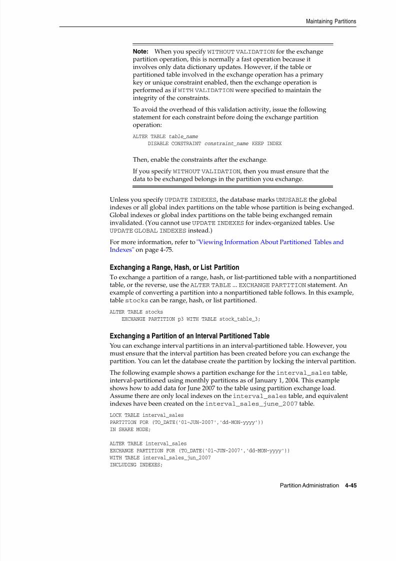
8/16/2019 Oracle Database VLDB and Partitioning Guide
http://slidepdf.com/reader/full/oracle-database-vldb-and-partitioning-guide 123/304
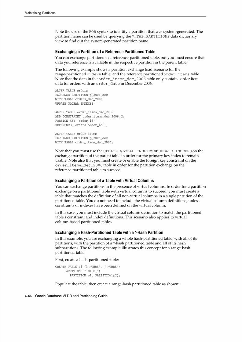
8/16/2019 Oracle Database VLDB and Partitioning Guide
http://slidepdf.com/reader/full/oracle-database-vldb-and-partitioning-guide 124/304
Maintaining Partitions
4-46 Oracle Database VLDB and Partitioning Guide
Note the use of the FOR syntax to identify a partition that was system-generated. Thepartition name can be used by querying the *_TAB_PARTITIONS data dictionaryview to find out the system-generated partition name.
Exchanging a Partition of a Reference Partitioned Table
You can exchange partitions in a reference-partitioned table, but you must ensure thatdata you reference is available in the respective partition in the parent table.
The following example shows a partition exchange load scenario for therange-partitioned orders table, and the reference partitioned order_items table.Note that the data in the order_items_dec_2006 table only contains order itemdata for orders with an order_date in December 2006.
ALTER TABLE ordersEXCHANGE PARTITION p_2006_dec
WITH TABLE orders_dec_2006UPDATE GLOBAL INDEXES;
ALTER TABLE order_items_dec_2006ADD CONSTRAINT order_items_dec_2006_fk
FOREIGN KEY (order_id)REFERENCES orders(order_id) ;
ALTER TABLE order_itemsEXCHANGE PARTITION p_2006_dec
WITH TABLE order_items_dec_2006;
Note that you must use the UPDATE GLOBAL INDEXES or UPDATE INDEXES on theexchange partition of the parent table in order for the primary key index to remainusable. Note also that you must create or enable the foreign key constraint on theorder_items_dec_2006 table in order for the partition exchange on thereference-partitioned table to succeed.
Exchanging a Partition of a Table with Virtual ColumnsYou can exchange partitions in the presence of virtual columns. In order for a partitionexchange on a partitioned table with virtual columns to succeed, you must create atable that matches the definition of all non-virtual columns in a single partition of thepartitioned table. You do not need to include the virtual column definitions, unlessconstraints or indexes have been defined on the virtual column.
In this case, you must include the virtual column definition to match the partitionedtable's constraint and index definitions. This scenario also applies to virtualcolumn-based partitioned tables.
Exchanging a Hash-Partitioned Table with a *-Hash Partition
In this example, you are exchanging a whole hash-partitioned table, with all of itspartitions, with the partition of a *-hash partitioned table and all of its hashsubpartitions. The following example illustrates this concept for a range-hashpartitioned table.
First, create a hash-partitioned table:
CREATE TABLE t1 (i NUMBER, j NUMBER) PARTITION BY HASH(i) (PARTITION p1, PARTITION p2);
Populate the table, then create a range-hash partitioned table as shown:
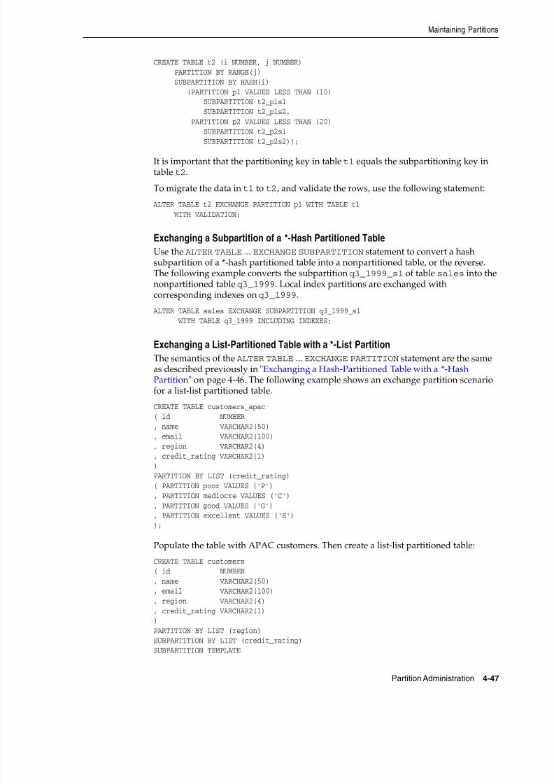
8/16/2019 Oracle Database VLDB and Partitioning Guide
http://slidepdf.com/reader/full/oracle-database-vldb-and-partitioning-guide 125/304
Maintaining Partitions
Partition Administration 4-47
CREATE TABLE t2 (i NUMBER, j NUMBER) PARTITION BY RANGE(j) SUBPARTITION BY HASH(i) (PARTITION p1 VALUES LESS THAN (10) SUBPARTITION t2_pls1 SUBPARTITION t2_pls2, PARTITION p2 VALUES LESS THAN (20) SUBPARTITION t2_p2s1 SUBPARTITION t2_p2s2));
It is important that the partitioning key in table t1 equals the subpartitioning key intable t2.
To migrate the data in t1 to t2, and validate the rows, use the following statement:
ALTER TABLE t2 EXCHANGE PARTITION p1 WITH TABLE t1 WITH VALIDATION;
Exchanging a Subpartition of a *-Hash Partitioned Table
Use the ALTER TABLE ... EXCHANGE SUBPARTITION statement to convert a hashsubpartition of a *-hash partitioned table into a nonpartitioned table, or the reverse.
The following example converts the subpartition q3_1999_s1 of table sales into thenonpartitioned table q3_1999. Local index partitions are exchanged withcorresponding indexes on q3_1999.
ALTER TABLE sales EXCHANGE SUBPARTITION q3_1999_s1 WITH TABLE q3_1999 INCLUDING INDEXES;
Exchanging a List-Partitioned Table with a *-List Partition
The semantics of the ALTER TABLE ... EXCHANGE PARTITION statement are the sameas described previously in "Exchanging a Hash-Partitioned Table with a *-HashPartition" on page 4-46. The following example shows an exchange partition scenariofor a list-list partitioned table.
CREATE TABLE customers_apac( id NUMBER, name VARCHAR2(50), email VARCHAR2(100), region VARCHAR2(4), credit_rating VARCHAR2(1))PARTITION BY LIST (credit_rating)( PARTITION poor VALUES ('P'), PARTITION mediocre VALUES ('C'), PARTITION good VALUES ('G'), PARTITION excellent VALUES ('E'));
Populate the table with APAC customers. Then create a list-list partitioned table:CREATE TABLE customers( id NUMBER, name VARCHAR2(50), email VARCHAR2(100), region VARCHAR2(4), credit_rating VARCHAR2(1))PARTITION BY LIST (region)SUBPARTITION BY LIST (credit_rating)SUBPARTITION TEMPLATE
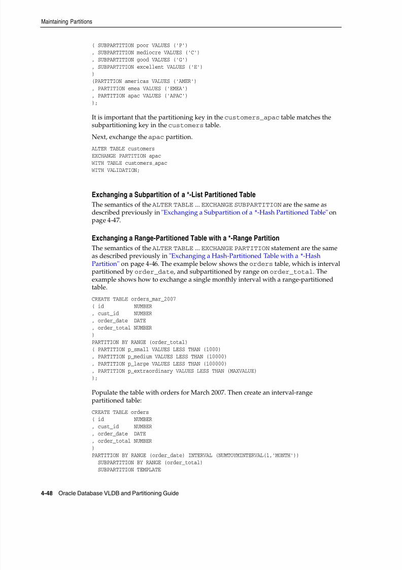
8/16/2019 Oracle Database VLDB and Partitioning Guide
http://slidepdf.com/reader/full/oracle-database-vldb-and-partitioning-guide 126/304
Maintaining Partitions
4-48 Oracle Database VLDB and Partitioning Guide
( SUBPARTITION poor VALUES ('P'), SUBPARTITION mediocre VALUES ('C'), SUBPARTITION good VALUES ('G'), SUBPARTITION excellent VALUES ('E'))(PARTITION americas VALUES ('AMER'), PARTITION emea VALUES ('EMEA'), PARTITION apac VALUES ('APAC'));
It is important that the partitioning key in the customers_apac table matches thesubpartitioning key in the customers table.
Next, exchange the apac partition.
ALTER TABLE customersEXCHANGE PARTITION apac
WITH TABLE customers_apac WITH VALIDATION;
Exchanging a Subpartition of a *-List Partitioned Table
The semantics of the ALTER TABLE ... EXCHANGE SUBPARTITION are the same asdescribed previously in "Exchanging a Subpartition of a *-Hash Partitioned Table" onpage 4-47.
Exchanging a Range-Partitioned Table with a *-Range Partition
The semantics of the ALTER TABLE ... EXCHANGE PARTITION statement are the sameas described previously in "Exchanging a Hash-Partitioned Table with a *-HashPartition" on page 4-46. The example below shows the orders table, which is intervalpartitioned by order_date, and subpartitioned by range on order_total. Theexample shows how to exchange a single monthly interval with a range-partitionedtable.
CREATE TABLE orders_mar_2007( id NUMBER, cust_id NUMBER, order_date DATE, order_total NUMBER)PARTITION BY RANGE (order_total)( PARTITION p_small VALUES LESS THAN (1000), PARTITION p_medium VALUES LESS THAN (10000), PARTITION p_large VALUES LESS THAN (100000), PARTITION p_extraordinary VALUES LESS THAN (MAXVALUE));
Populate the table with orders for March 2007. Then create an interval-range
partitioned table:
CREATE TABLE orders( id NUMBER, cust_id NUMBER, order_date DATE, order_total NUMBER)PARTITION BY RANGE (order_date) INTERVAL (NUMTOYMINTERVAL(1,'MONTH')) SUBPARTITION BY RANGE (order_total) SUBPARTITION TEMPLATE
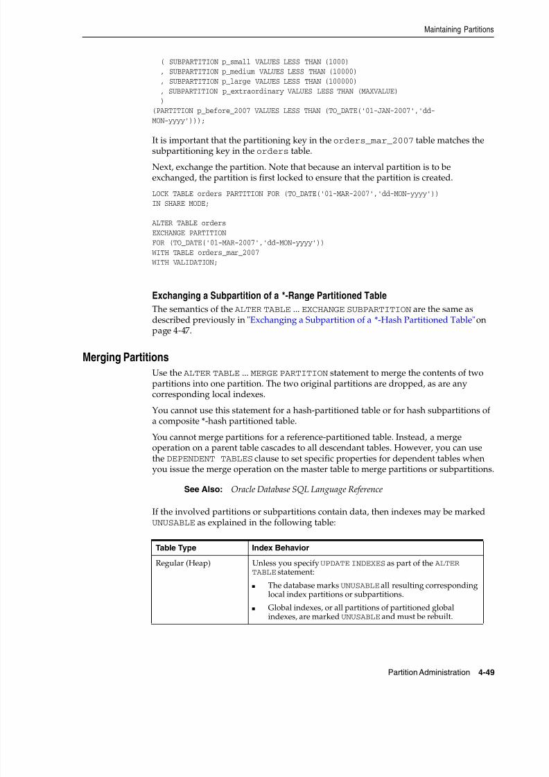
8/16/2019 Oracle Database VLDB and Partitioning Guide
http://slidepdf.com/reader/full/oracle-database-vldb-and-partitioning-guide 127/304
Maintaining Partitions
Partition Administration 4-49
( SUBPARTITION p_small VALUES LESS THAN (1000) , SUBPARTITION p_medium VALUES LESS THAN (10000) , SUBPARTITION p_large VALUES LESS THAN (100000) , SUBPARTITION p_extraordinary VALUES LESS THAN (MAXVALUE) )(PARTITION p_before_2007 VALUES LESS THAN (TO_DATE('01-JAN-2007','dd-MON-yyyy')));
It is important that the partitioning key in the orders_mar_2007 table matches thesubpartitioning key in the orders table.
Next, exchange the partition. Note that because an interval partition is to beexchanged, the partition is first locked to ensure that the partition is created.
LOCK TABLE orders PARTITION FOR (TO_DATE('01-MAR-2007','dd-MON-yyyy'))IN SHARE MODE;
ALTER TABLE ordersEXCHANGE PARTITIONFOR (TO_DATE('01-MAR-2007','dd-MON-yyyy'))
WITH TABLE orders_mar_2007 WITH VALIDATION;
Exchanging a Subpartition of a *-Range Partitioned Table
The semantics of the ALTER TABLE ... EXCHANGE SUBPARTITION are the same asdescribed previously in "Exchanging a Subpartition of a *-Hash Partitioned Table" onpage 4-47.
Merging PartitionsUse the ALTER TABLE ... MERGE PARTITION statement to merge the contents of twopartitions into one partition. The two original partitions are dropped, as are anycorresponding local indexes.
You cannot use this statement for a hash-partitioned table or for hash subpartitions ofa composite *-hash partitioned table.
You cannot merge partitions for a reference-partitioned table. Instead, a mergeoperation on a parent table cascades to all descendant tables. However, you can usethe DEPENDENT TABLES clause to set specific properties for dependent tables whenyou issue the merge operation on the master table to merge partitions or subpartitions.
If the involved partitions or subpartitions contain data, then indexes may be markedUNUSABLE as explained in the following table:
See Also: Oracle Database SQL Language Reference
Table Type Index Behavior
Regular (Heap) Unless you specify UPDATE INDEXES as part of the ALTER TABLE statement:
■ The database marks UNUSABLE all resulting correspondinglocal index partitions or subpartitions.
■ Global indexes, or all partitions of partitioned globalindexes, are marked UNUSABLE and must be rebuilt.
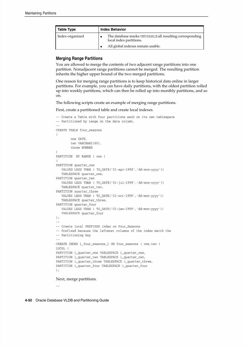
8/16/2019 Oracle Database VLDB and Partitioning Guide
http://slidepdf.com/reader/full/oracle-database-vldb-and-partitioning-guide 128/304
Maintaining Partitions
4-50 Oracle Database VLDB and Partitioning Guide
Merging Range PartitionsYou are allowed to merge the contents of two adjacent range partitions into onepartition. Nonadjacent range partitions cannot be merged. The resulting partitioninherits the higher upper bound of the two merged partitions.
One reason for merging range partitions is to keep historical data online in largerpartitions. For example, you can have daily partitions, with the oldest partition rolledup into weekly partitions, which can then be rolled up into monthly partitions, and soon.
The following scripts create an example of merging range partitions.
First, create a partitioned table and create local indexes.
-- Create a Table with four partitions each on its own tablespace
-- Partitioned by range on the data column.--CREATE TABLE four_seasons(
one DATE, two VARCHAR2(60), three NUMBER)PARTITION BY RANGE ( one )(PARTITION quarter_one VALUES LESS THAN ( TO_DATE('01-apr-1998','dd-mon-yyyy'))
TABLESPACE quarter_one,PARTITION quarter_two
VALUES LESS THAN ( TO_DATE('01-jul-1998','dd-mon-yyyy')) TABLESPACE quarter_two,PARTITION quarter_three VALUES LESS THAN ( TO_DATE('01-oct-1998','dd-mon-yyyy')) TABLESPACE quarter_three,PARTITION quarter_four VALUES LESS THAN ( TO_DATE('01-jan-1999','dd-mon-yyyy')) TABLESPACE quarter_four);---- Create local PREFIXED index on Four_Seasons-- Prefixed because the leftmost columns of the index match the-- Partitioning key--
CREATE INDEX i_four_seasons_l ON four_seasons ( one,two )LOCAL (PARTITION i_quarter_one TABLESPACE i_quarter_one,PARTITION i_quarter_two TABLESPACE i_quarter_two,PARTITION i_quarter_three TABLESPACE i_quarter_three,PARTITION i_quarter_four TABLESPACE i_quarter_four);
Next, merge partitions.
--
Index-organized ■ The database marks UNUSABLE all resulting correspondinglocal index partitions.
■ All global indexes remain usable.
Table Type Index Behavior

8/16/2019 Oracle Database VLDB and Partitioning Guide
http://slidepdf.com/reader/full/oracle-database-vldb-and-partitioning-guide 129/304
Maintaining Partitions
Partition Administration 4-51
-- Merge the first two partitions--ALTER TABLE four_seasonsMERGE PARTITIONS quarter_one, quarter_two INTO PARTITION quarter_twoUPDATE INDEXES;
If you omit the UPDATE INDEXES clause from the preceding statement, then you must
rebuild the local index for the affected partition.-- Rebuild index for quarter_two, which has been marked unusable-- because it has not had all of the data from Q1 added to it.-- Rebuilding the index corrects this.--ALTER TABLE four_seasons MODIFY PARTITIONquarter_two REBUILD UNUSABLE LOCAL INDEXES;
Merging Interval Partitions
The contents of two adjacent interval partitions can be merged into one partition.Nonadjacent interval partitions cannot be merged. The first interval partition can also be merged with the highest range partition. The resulting partition inherits the higherupper bound of the two merged partitions.
Merging interval partitions always results in the transition point being moved to thehigher upper bound of the two merged partitions. This result is that the range sectionof the interval-partitioned table is extended to the upper bound of the two mergedpartitions. Any materialized interval partitions with boundaries lower than the newlymerged partition is automatically be converted into range partitions, with their upper boundaries defined by the upper boundaries of their intervals.
For example, consider the following interval-partitioned table transactions:
CREATE TABLE transactions( id NUMBER, transaction_date DATE, value NUMBER
)PARTITION BY RANGE (transaction_date)INTERVAL (NUMTODSINTERVAL(1,'DAY'))( PARTITION p_before_2007 VALUES LESS THAN (TO_DATE('01-JAN-2007','dd-MON-yyyy')));
Insert data into the interval section of the table. This creates the interval partitions forthese days. Note that January 15, 2007 and January 16, 2007 are stored in adjacentinterval partitions.
INSERT INTO transactions VALUES (1,TO_DATE('15-JAN-2007','dd-MON-yyyy'),100);INSERT INTO transactions VALUES (2,TO_DATE('16-JAN-2007','dd-MON-yyyy'),600);INSERT INTO transactions VALUES (3,TO_DATE('30-JAN-2007','dd-MON-yyyy'),200);
Next, merge the two adjacent interval partitions. The new partition again has asystem-generated name.
ALTER TABLE transactionsMERGE PARTITIONS FOR(TO_DATE('15-JAN-2007','dd-MON-yyyy')), FOR(TO_DATE('16-JAN-2007','dd-MON-yyyy'));
The transition point for the transactions table has now moved to January 17, 2007.The range section of the interval-partitioned table contains two range partitions:values less than January 1, 2007 and values less than January 17, 2007. Values greaterthan January 17, 2007 fall in the interval portion of the interval-partitioned table.
8/16/2019 Oracle Database VLDB and Partitioning Guide
http://slidepdf.com/reader/full/oracle-database-vldb-and-partitioning-guide 130/304
Maintaining Partitions
4-52 Oracle Database VLDB and Partitioning Guide
Merging List Partitions
When you merge list partitions, the partitions being merged can be any two partitions.They do not need to be adjacent, as for range partitions, because list partitioning doesnot assume any order for partitions. The resulting partition consists of all of the datafrom the original two partitions. If you merge a default list partition with any otherpartition, the resulting partition is the default partition.
The following statement merges two partitions of a table partitioned using the listmethod into a partition that inherits all of its attributes from the table-level defaultattributes. MAXEXTENTS is specified in the statement.
ALTER TABLE q1_sales_by_regionMERGE PARTITIONS q1_northcentral, q1_southcentralINTO PARTITION q1_central
STORAGE(MAXEXTENTS 20);
The value lists for the two original partitions were specified as:
PARTITION q1_northcentral VALUES ('SD','WI')PARTITION q1_southcentral VALUES ('OK','TX')
The resulting sales_west partition value list comprises the set that represents theunion of these two partition value lists, or specifically:
('SD','WI','OK','TX')
Merging *-Hash Partitions
When you merge *-hash partitions, the subpartitions are rehashed into the number ofsubpartitions specified by SUBPARTITIONS n or the SUBPARTITION clause. If neitheris included, table-level defaults are used.
Note that the inheritance of properties is different when a *-hash partition is split(discussed in "Splitting a *-Hash Partition" on page 4-66), as opposed to when two*-hash partitions are merged. When a partition is split, the new partitions can inheritproperties from the original partition because there is only one parent. However, when
partitions are merged, properties must be inherited from the table level.
For interval-hash partitioned tables, you can only merge two adjacent intervalpartitions, or the highest range partition with the first interval partition. As describedin "Merging Interval Partitions" on page 4-51, the transition point moves when youmerge intervals in an interval-hash partitioned table.
The following example merges two range-hash partitions:
ALTER TABLE all_seasons MERGE PARTITIONS quarter_1, quarter_2 INTO PARTITION quarter_2 SUBPARTITIONS 8;
Merging *-List Partitions
Partitions can be merged at the partition level and subpartitions can be merged at thelist subpartition level.
Merging Partitions in a *-List Partitioned Table Merging partitions in a *-list partitionedtable is as described previously in "Merging Range Partitions" on page 4-50. However,when you merge two *-list partitions, the resulting new partition inherits thesubpartition descriptions from the subpartition template, if one exists. If nosubpartition template exists, then a single default subpartition is created for the newpartition.

8/16/2019 Oracle Database VLDB and Partitioning Guide
http://slidepdf.com/reader/full/oracle-database-vldb-and-partitioning-guide 131/304
Maintaining Partitions
Partition Administration 4-53
For interval-list partitioned tables, you can only merge two adjacent intervalpartitions, or the highest range partition with the first interval partition. As describedin "Merging Interval Partitions" on page 4-51, the transition point moves when youmerge intervals in an interval-list partitioned table.
The following statement merges two partitions in the range-list partitioned stripe_regional_sales table. A subpartition template exists for the table.
ALTER TABLE stripe_regional_sales MERGE PARTITIONS q1_1999, q2_1999 INTO PARTITION q1_q2_1999 STORAGE(MAXEXTENTS 20);
Some new physical attributes are specified for this new partition while table-leveldefaults are inherited for those that are not specified. The new resulting partition q1_q2_1999 inherits the high-value bound of the partition q2_1999 and the subpartitionvalue-list descriptions from the subpartition template description of the table.
The data in the resulting partitions consists of data from both the partitions. However,there may be cases where the database returns an error. This can occur because datamay map out of the new partition when both of the following conditions exist:
■ Some literal values of the merged subpartitions were not included in the
subpartition template.
■ The subpartition template does not contain a default partition definition.
This error condition can be eliminated by always specifying a default partition in thedefault subpartition template.
Merging Subpartitions in a *-List Partitioned Table You can merge the contents of any twoarbitrary list subpartitions belonging to the same partition. The resulting subpartitionvalue-list descriptor includes all of the literal values in the value lists for the partitions being merged.
The following statement merges two subpartitions of a table partitioned usingrange-list method into a new subpartition located in tablespace ts4:
ALTER TABLE quarterly_regional_sales MERGE SUBPARTITIONS q1_1999_northwest, q1_1999_southwest INTO SUBPARTITION q1_1999_west TABLESPACE ts4;
The value lists for the original two partitions were:
■ Subpartition q1_1999_northwest was described as ('WA','OR')
■ Subpartition q1_1999_southwest was described as ('AZ','NM','UT')
The resulting subpartition value list comprises the set that represents the union ofthese two subpartition value lists:
■ Subpartition q1_1999_west has a value list described as
('WA','OR','AZ','NM','UT')
The tablespace in which the resulting subpartition is located and the subpartitionattributes are determined by the partition-level default attributes, except for thosespecified explicitly. If any of the existing subpartition names are being reused, then thenew subpartition inherits the subpartition attributes of the subpartition whose name is being reused.
8/16/2019 Oracle Database VLDB and Partitioning Guide
http://slidepdf.com/reader/full/oracle-database-vldb-and-partitioning-guide 132/304
Maintaining Partitions
4-54 Oracle Database VLDB and Partitioning Guide
Merging *-Range Partitions
Partitions can be merged at the partition level and subpartitions can be merged at therange subpartition level.
Merging Partitions in a *-Range Partitioned Table Merging partitions in a *-range partitionedtable is as described previously in "Merging Range Partitions" on page 4-50. However,when you merge two *-range partitions, the resulting new partition inherits thesubpartition descriptions from the subpartition template, if one exists. If nosubpartition template exists, then a single subpartition with an upper boundaryMAXVALUE is created for the new partition.
For interval-range partitioned tables, you can only merge two adjacent intervalpartitions, or the highest range partition with the first interval partition. As describedin "Merging Interval Partitions" on page 4-51, the transition point moves when youmerge intervals in an interval-range partitioned table.
The following statement merges two partitions in the monthly interval-rangepartitioned orders table. A subpartition template exists for the table.
ALTER TABLE ordersMERGE PARTITIONS FOR(TO_DATE('01-MAR-2007','dd-MON-yyyy')),
FOR(TO_DATE('01-APR-2007','dd-MON-yyyy'))INTO PARTITION p_pre_may_2007;
If the March 2007 and April 2007 partitions were still in the interval section of theinterval-range partitioned table, then the merge operation would move the transitionpoint to May 1, 2007.
The subpartitions for partition p_pre_may_2007 inherit their properties from thesubpartition template. The data in the resulting partitions consists of data from boththe partitions. However, there may be cases where the database returns an error. Thiscan occur because data may map out of the new partition when both of the followingconditions are met:
■ Some range values of the merged subpartitions were not included in the
subpartition template.
■ The subpartition template does not have a subpartition definition with aMAXVALUE upper boundary.
The error condition can be eliminated by always specifying a subpartition with anupper boundary of MAXVALUE in the subpartition template.
Modifying Default AttributesYou can modify the default attributes of a table, or for a partition of a compositepartitioned table. When you modify default attributes, the new attributes affect onlyfuture partitions, or subpartitions, that are created. The default values can still bespecifically overridden when creating a new partition or subpartition. You can modify
the default attributes of a reference-partitioned table.
Modifying Default Attributes of a Table
You can modify the default attributes that are inherited for range, hash, list, interval,or reference partitions using the MODIFY DEFAULT ATTRIBUTES clause of ALTER TABLE.
For hash-partitioned tables, only the TABLESPACE attribute can be modified.
8/16/2019 Oracle Database VLDB and Partitioning Guide
http://slidepdf.com/reader/full/oracle-database-vldb-and-partitioning-guide 133/304
Maintaining Partitions
Partition Administration 4-55
Modifying Default Attributes of a Partition
To modify the default attributes inherited when creating subpartitions, use the ALTER TABLE ... MODIFY DEFAULT ATTRIBUTES FOR PARTITION. The following statementmodifies the TABLESPACE in which future subpartitions of partition p1 in range-hashpartitioned table emp reside.
ALTER TABLE emp
MODIFY DEFAULT ATTRIBUTES FOR PARTITION p1 TABLESPACE ts1;
Because all subpartitions of a range-hash partitioned table must share the sameattributes, except TABLESPACE, it is the only attribute that can be changed.
You cannot modify default attributes of interval partitions that have not yet beencreated. To change the way in which future subpartitions in an interval-partitionedtable are created, then you must modify the subpartition template.
Modifying Default Attributes of Index Partitions
In similar fashion to table partitions, you can alter the default attributes that areinherited by partitions of a range-partitioned global index, or local index partitions ofpartitioned tables. For this you use the ALTER INDEX ... MODIFY DEFAULT
ATTRIBUTES statement. Use the ALTER INDEX ... MODIFY DEFAULT ATTRIBUTES FOR PARTITION statement if you are altering default attributes to be inherited bysubpartitions of a composite partitioned table.
Modifying Real Attributes of PartitionsIt is possible to modify attributes of an existing partition of a table or index.
You cannot change the TABLESPACE attribute. Use ALTER TABLE ... MOVE PARTITION/SUBPARTITION to move a partition or subpartition to a new tablespace.
Modifying Real Attributes for a Range or List Partition
Use the ALTER TABLE ... MODIFY PARTITION statement to modify existing attributes
of a range partition or list partition. You can modify segment attributes (exceptTABLESPACE), or you can allocate and deallocate extents, mark local index partitionsUNUSABLE, or rebuild local indexes that have been marked UNUSABLE.
If this is a range partition of a *-hash partitioned table, then note the following:
■ If you allocate or deallocate an extent, this action is performed for everysubpartition of the specified partition.
■ Likewise, changing any other attributes results in corresponding changes to thoseattributes of all the subpartitions for that partition. The partition level defaultattributes are changed as well. To avoid changing attributes of existingsubpartitions, use the FOR PARTITION clause of the MODIFY DEFAULT ATTRIBUTES statement.
The following are some examples of modifying the real attributes of a partition.
This example modifies the MAXEXTENTS storage attribute for the range partitionsales_q1 of table sales:
ALTER TABLE sales MODIFY PARTITION sales_q1 STORAGE (MAXEXTENTS 10);
All of the local index subpartitions of partition ts1 in range-hash partitioned tablescubagear are marked UNUSABLE in the following example:
8/16/2019 Oracle Database VLDB and Partitioning Guide
http://slidepdf.com/reader/full/oracle-database-vldb-and-partitioning-guide 134/304
Maintaining Partitions
4-56 Oracle Database VLDB and Partitioning Guide
ALTER TABLE scubagear MODIFY PARTITION ts1 UNUSABLE LOCAL INDEXES;
For an interval-partitioned table you can only modify real attributes of range partitionsor interval partitions that have been created.
Modifying Real Attributes for a Hash Partition
You also use the ALTER TABLE ... MODIFY PARTITION statement to modify attributes
of a hash partition. However, because the physical attributes of individual hashpartitions must all be the same (except for TABLESPACE), you are restricted to:
■ Allocating a new extent
■ Deallocating an unused extent
■ Marking a local index subpartition UNUSABLE
■ Rebuilding local index subpartitions that are marked UNUSABLE
The following example rebuilds any unusable local index partitions associated withhash partition P1 of table dept:
ALTER TABLE dept MODIFY PARTITION p1 REBUILD UNUSABLE LOCAL INDEXES;
Modifying Real Attributes of a Subpartition
With the MODIFY SUBPARTITION clause of ALTER TABLE you can perform the sameactions as listed previously for partitions, but at the specific composite partitionedtable subpartition level. For example:
ALTER TABLE emp MODIFY SUBPARTITION p3_s1 REBUILD UNUSABLE LOCAL INDEXES;
Modifying Real Attributes of Index Partitions
The MODIFY PARTITION clause of ALTER INDEX lets you modify the real attributes ofan index partition or its subpartitions. The rules are very similar to those for tablepartitions, but unlike the MODIFY PARTITION clause for ALTER INDEX, there is nosubclause to rebuild an unusable index partition, but there is a subclause to coalescean index partition or its subpartitions. In this context, coalesce means to merge index blocks where possible to free them for reuse.
You can also allocate or deallocate storage for a subpartition of a local index, or mark itUNUSABLE, using the MODIFY PARTITION clause.
Modifying List Partitions: Adding ValuesList partitioning enables you to optionally add literal values from the defining valuelist.
Adding Values for a List Partition
Use the MODIFY PARTITION ... ADD VALUES clause of the ALTER TABLE statement toextend the value list of an existing partition. Literal values being added must not have been included in any other partition value list. The partition value list for anycorresponding local index partition is correspondingly extended, and any globalindexes, or global or local index partitions, remain usable.
The following statement adds a new set of state codes ('OK', 'KS') to an existingpartition list.
ALTER TABLE sales_by_region MODIFY PARTITION region_south

8/16/2019 Oracle Database VLDB and Partitioning Guide
http://slidepdf.com/reader/full/oracle-database-vldb-and-partitioning-guide 135/304
Maintaining Partitions
Partition Administration 4-57
ADD VALUES ('OK', 'KS');
The existence of a default partition can have a performance impact when addingvalues to other partitions. This is because to add values to a list partition, the databasemust check that the values being added do not exist in the default partition. If any ofthe values do exist in the default partition, then an error is raised.
You cannot add values to a default list partition.
Adding Values for a List Subpartition
This operation is essentially the same as described for "Modifying List Partitions:Adding Values", however, you use a MODIFY SUBPARTITION clause instead of the
MODIFY PARTITION clause. For example, to extend the range of literal values in thevalue list for subpartition q1_1999_southeast, use the following statement:
ALTER TABLE quarterly_regional_sales MODIFY SUBPARTITION q1_1999_southeast ADD VALUES ('KS');
Literal values being added must not have been included in any other subpartitionvalue list within the owning partition. However, they can be duplicates of literalvalues in the subpartition value lists of other partitions within the table.
For an interval-list composite partitioned table, you can only add values tosubpartitions of range partitions or interval partitions that have been created. To addvalues to subpartitions of interval partitions that have not yet been created, then you
must modify the subpartition template.
Modifying List Partitions: Dropping ValuesList partitioning enables you to optionally drop literal values from the defining valuelist.
Dropping Values from a List Partition
Use the MODIFY PARTITION ... DROP VALUES clause of the ALTER TABLE statement toremove literal values from the value list of an existing partition. The statement isalways executed with validation, meaning that it checks to see if any rows exist in thepartition that corresponds to the set of values being dropped. If any such rows are
found then the database returns an error message and the operation fails. Whennecessary, use a DELETE statement to delete corresponding rows from the table beforeattempting to drop values.
Note: The database executes a query to check for the existence ofrows in the default partition that correspond to the literal values beingadded. Therefore, it is advisable to create a local prefixed index on thetable. This speeds up the execution of the query and the overalloperation.
Note: You cannot drop all literal values from the value list describingthe partition. You must use the ALTER TABLE ... DROPPARTITION statement instead.

8/16/2019 Oracle Database VLDB and Partitioning Guide
http://slidepdf.com/reader/full/oracle-database-vldb-and-partitioning-guide 136/304
Maintaining Partitions
4-58 Oracle Database VLDB and Partitioning Guide
The partition value list for any corresponding local index partition reflects the newvalue list, and any global index, or global or local index partitions, remain usable.
The following statement drops a set of state codes ('OK' and 'KS') from an existingpartition value list.
ALTER TABLE sales_by_region MODIFY PARTITION region_south
DROP VALUES ('OK', 'KS');
You cannot drop values from a default list partition.
Dropping Values from a List Subpartition
This operation is essentially the same as described for "Modifying List Partitions:Dropping Values", however, you use a MODIFY SUBPARTITION clause instead of theMODIFY PARTITION clause. For example, to remove a set of literal values in the valuelist for subpartition q1_1999_southeast, use the following statement:
ALTER TABLE quarterly_regional_sales MODIFY SUBPARTITION q1_1999_southeast DROP VALUES ('KS');
For an interval-list composite partitioned table, you can only drop values fromsubpartitions of range partitions or interval partitions that have been created. To dropvalues from subpartitions of interval partitions that have not yet been created, youmust modify the subpartition template.
Modifying a Subpartition TemplateYou can modify a subpartition template of a composite partitioned table by replacing itwith a new subpartition template. Any subsequent operations that use thesubpartition template (such as ADD PARTITION or MERGE PARTITIONS) now use thenew subpartition template. Existing subpartitions remain unchanged.
If you modify a subpartition template of an interval-* composite partitioned table, theninterval partitions that have not yet been created use the new subpartition template.
Use the ALTER TABLE ... SET SUBPARTITION TEMPLATE statement to specify a newsubpartition template. For example:
ALTER TABLE emp_sub_template
SET SUBPARTITION TEMPLATE (SUBPARTITION e TABLESPACE ts1, SUBPARTITION f TABLESPACE ts2, SUBPARTITION g TABLESPACE ts3, SUBPARTITION h TABLESPACE ts4 );
You can drop a subpartition template by specifying an empty list:
ALTER TABLE emp_sub_template SET SUBPARTITION TEMPLATE ( );
Note: The database executes a query to check for the existence ofrows in the partition that correspond to the literal values beingdropped. Therefore, it is advisable to create a local prefixed index onthe table. This speeds up the execution of the query and the overalloperation.
8/16/2019 Oracle Database VLDB and Partitioning Guide
http://slidepdf.com/reader/full/oracle-database-vldb-and-partitioning-guide 137/304
Maintaining Partitions
Partition Administration 4-59
Moving PartitionsUse the MOVE PARTITION clause of the ALTER TABLE statement to:
■ Re-cluster data and reduce fragmentation
■ Move a partition to another tablespace
■ Modify create-time attributes
■ Store the data in compressed format using table compression
Typically, you can change the physical storage attributes of a partition in a single stepusing an ALTER TABLE/INDEX ... MODIFY PARTITION statement. However, there aresome physical attributes, such as TABLESPACE, that you cannot modify using MODIFY PARTITION. In these cases, use the MOVE PARTITION clause. Modifying some otherattributes, such as table compression, affects only future storage, but not existing data.
If the partition being moved contains any data, indexes may be marked UNUSABLE according to the following table:
Moving Table Partitions
Use the MOVE PARTITION clause to move a partition. For example, to move the mostactive partition to a tablespace that resides on its own set of disks (to balance I/O), notlog the action, and compress the data, issue the following statement:
ALTER TABLE parts MOVE PARTITION depot2 TABLESPACE ts094 NOLOGGING COMPRESS;
This statement always drops the old partition segment and creates a new segment,even if you do not specify a new tablespace.
If you are moving a partition of a partitioned index-organized table, then you canspecify the MAPPING TABLE clause as part of the MOVE PARTITION clause, and themapping table partition are moved to the new location along with the table partition.
For an interval or interval-* partitioned table, you can only move range partitions orinterval partitions that have been created. A partition move operation does not movethe transition point in an interval or interval-* partitioned table.
Note: ALTER TABLE...MOVE does not permit DML on the partitionwhile the command is executing. To move a partition and leave itavailable for DML, see "Redefining Partitions Online" on page 4-60.
Table Type Index Behavior
Regular (Heap) Unless you specify UPDATE INDEXES as part of the ALTER TABLE statement:
■ The matching partition in each local index is markedUNUSABLE. You must rebuild these index partitions afterissuing MOVE PARTITION.
■ Any global indexes, or all partitions of partitioned globalindexes, are marked UNUSABLE.
Index-organized Any local or global indexes defined for the partition beingmoved remain usable because they are primary-key basedlogical rowids. However, the guess information for these rowids
becomes incorrect.
8/16/2019 Oracle Database VLDB and Partitioning Guide
http://slidepdf.com/reader/full/oracle-database-vldb-and-partitioning-guide 138/304
Maintaining Partitions
4-60 Oracle Database VLDB and Partitioning Guide
You can move a partition in a reference-partitioned table independent of the partitionin the master table.
Moving Subpartitions
The following statement shows how to move data in a subpartition of a table. In thisexample, a PARALLEL clause has also been specified.
ALTER TABLE scuba_gear MOVE SUBPARTITION bcd_typesTABLESPACE tbs23 PARALLEL (DEGREE 2);
You can move a subpartition in a reference-partitioned table independent of thesubpartition in the master table.
Moving Index Partitions
The ALTER TABLE ... MOVE PARTITION statement for regular tables, marks allpartitions of a global index UNUSABLE. You can rebuild the entire index by rebuildingeach partition individually using the ALTER INDEX ... REBUILD PARTITION statement. You can perform these rebuilds concurrently.
You can also simply drop the index and re-create it.
Redefining Partitions OnlineOracle Database provides a mechanism to move a partition or to make other changesto the partition's physical structure without significantly affecting the availability ofthe partition for DML. This mechanism is called online table redefinition.
For information about redefining a single partition of a table, see Oracle Database Administrator's Guide.
Redefining Partitions with Collection Tables
You can use online redefinition to copy over nonpartitioned Collection Tables topartitioned Collection Tables and Oracle Database inserts rows into the appropriatepartitions in the Collection Table. The example below illustrates how this is done fornested tables inside an Objects column; a similar example works for OrderedCollection Type Tables inside an XMLType table or column. Note that during thecopy_table_dependents operation, you specify 0 or false for copying the indexesand constraints, as you want to keep the indexes and constraints of the newly definedcollection table. However, it is important to note that the Collection Tables and itspartitions have the same names as that of the interim table (print_media2 in theexample below). You must take explicit steps to preserve the Collection Table names.
CONNECT / AS SYSDBADROP USER eqnt CASCADE;CREATE USER eqnt IDENTIFIED BY eqnt;GRANT CONNECT, RESOURCE TO eqnt;
-- Grant privleges required for online redefinition.GRANT EXECUTE ON DBMS_REDEFINITION TO eqnt;GRANT ALTER ANY TABLE TO eqnt;GRANT DROP ANY TABLE TO eqnt;GRANT LOCK ANY TABLE TO eqnt;GRANT CREATE ANY TABLE TO eqnt;GRANT SELECT ANY TABLE TO eqnt; -- Privileges required to perform cloning of dependent objects.GRANT CREATE ANY TRIGGER TO eqnt;
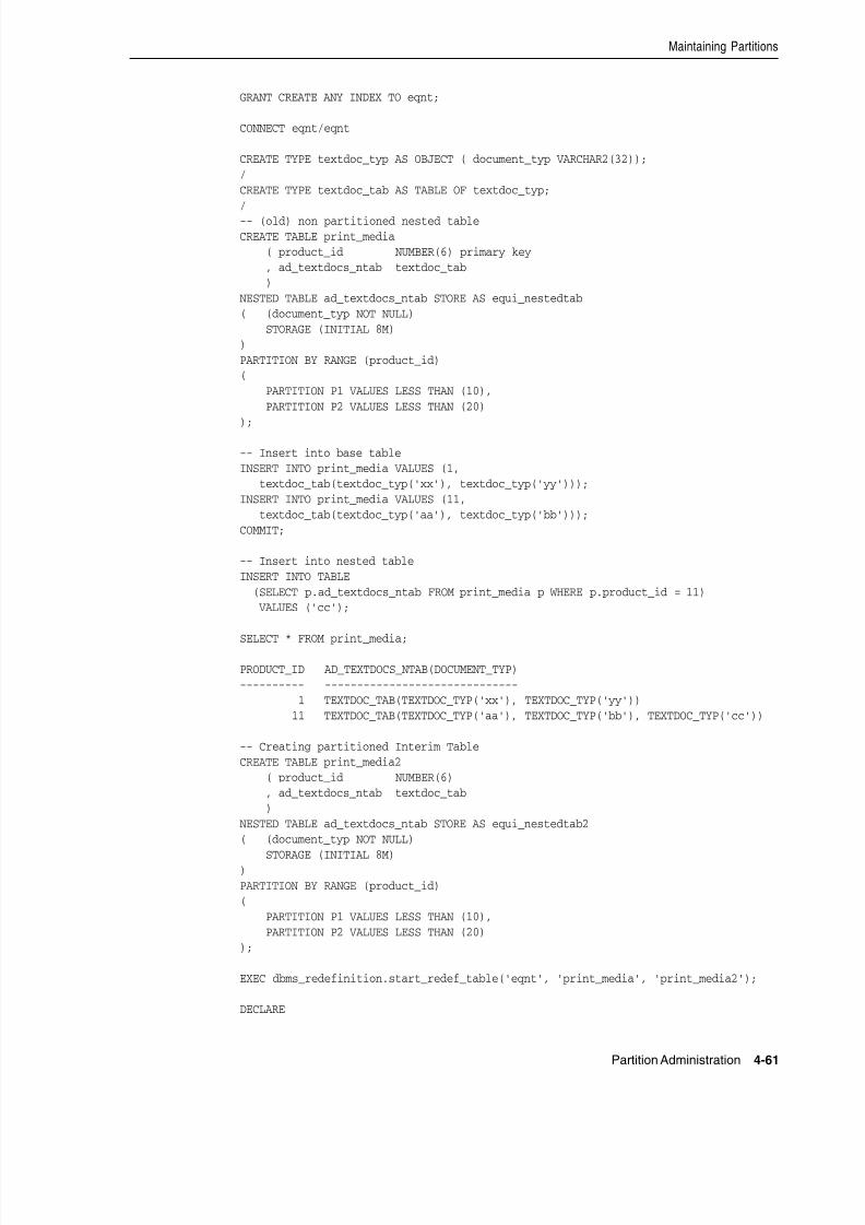
8/16/2019 Oracle Database VLDB and Partitioning Guide
http://slidepdf.com/reader/full/oracle-database-vldb-and-partitioning-guide 139/304
Maintaining Partitions
Partition Administration 4-61
GRANT CREATE ANY INDEX TO eqnt; CONNECT eqnt/eqnt CREATE TYPE textdoc_typ AS OBJECT ( document_typ VARCHAR2(32));/CREATE TYPE textdoc_tab AS TABLE OF textdoc_typ;/-- (old) non partitioned nested tableCREATE TABLE print_media ( product_id NUMBER(6) primary key , ad_textdocs_ntab textdoc_tab )NESTED TABLE ad_textdocs_ntab STORE AS equi_nestedtab( (document_typ NOT NULL) STORAGE (INITIAL 8M))PARTITION BY RANGE (product_id)( PARTITION P1 VALUES LESS THAN (10), PARTITION P2 VALUES LESS THAN (20)); -- Insert into base tableINSERT INTO print_media VALUES (1, textdoc_tab(textdoc_typ('xx'), textdoc_typ('yy')));INSERT INTO print_media VALUES (11, textdoc_tab(textdoc_typ('aa'), textdoc_typ('bb')));COMMIT; -- Insert into nested tableINSERT INTO TABLE (SELECT p.ad_textdocs_ntab FROM print_media p WHERE p.product_id = 11) VALUES ('cc');
SELECT * FROM print_media;
PRODUCT_ID AD_TEXTDOCS_NTAB(DOCUMENT_TYP)---------- ------------------------------ 1 TEXTDOC_TAB(TEXTDOC_TYP('xx'), TEXTDOC_TYP('yy')) 11 TEXTDOC_TAB(TEXTDOC_TYP('aa'), TEXTDOC_TYP('bb'), TEXTDOC_TYP('cc')) -- Creating partitioned Interim TableCREATE TABLE print_media2 ( product_id NUMBER(6) , ad_textdocs_ntab textdoc_tab )NESTED TABLE ad_textdocs_ntab STORE AS equi_nestedtab2( (document_typ NOT NULL)
STORAGE (INITIAL 8M))PARTITION BY RANGE (product_id)( PARTITION P1 VALUES LESS THAN (10), PARTITION P2 VALUES LESS THAN (20)); EXEC dbms_redefinition.start_redef_table('eqnt', 'print_media', 'print_media2'); DECLARE

8/16/2019 Oracle Database VLDB and Partitioning Guide
http://slidepdf.com/reader/full/oracle-database-vldb-and-partitioning-guide 140/304
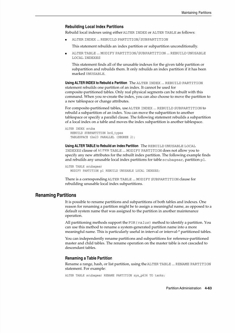
8/16/2019 Oracle Database VLDB and Partitioning Guide
http://slidepdf.com/reader/full/oracle-database-vldb-and-partitioning-guide 141/304
Maintaining Partitions
Partition Administration 4-63
Rebuilding Local Index Partitions
Rebuild local indexes using either ALTER INDEX or ALTER TABLE as follows:
■ ALTER INDEX ... REBUILD PARTITION/SUBPARTITION
This statement rebuilds an index partition or subpartition unconditionally.
■ ALTER TABLE ... MODIFY PARTITION/SUBPARTITION ... REBUILD UNUSABLE
LOCAL INDEXES This statement finds all of the unusable indexes for the given table partition orsubpartition and rebuilds them. It only rebuilds an index partition if it has beenmarked UNUSABLE.
Using ALTER INDEX to Rebuild a Partition The ALTER INDEX ... REBUILD PARTITION statement rebuilds one partition of an index. It cannot be used forcomposite-partitioned tables. Only real physical segments can be rebuilt with thiscommand. When you re-create the index, you can also choose to move the partition toa new tablespace or change attributes.
For composite-partitioned tables, use ALTER INDEX ... REBUILD SUBPARTITION torebuild a subpartition of an index. You can move the subpartition to another
tablespace or specify a parallel clause. The following statement rebuilds a subpartitionof a local index on a table and moves the index subpartition is another tablespace.
ALTER INDEX scuba REBUILD SUBPARTITION bcd_types TABLESPACE tbs23 PARALLEL (DEGREE 2);
Using ALTER TABLE to Rebuild an Index Partition The REBUILD UNUSABLE LOCAL INDEXES clause of ALTER TABLE ... MODIFY PARTITION does not allow you tospecify any new attributes for the rebuilt index partition. The following example findsand rebuilds any unusable local index partitions for table scubagear, partition p1.
ALTER TABLE scubagear MODIFY PARTITION p1 REBUILD UNUSABLE LOCAL INDEXES;
There is a corresponding ALTER TABLE ... MODIFY SUBPARTITION clause forrebuilding unusable local index subpartitions.
Renaming PartitionsIt is possible to rename partitions and subpartitions of both tables and indexes. Onereason for renaming a partition might be to assign a meaningful name, as opposed to adefault system name that was assigned to the partition in another maintenanceoperation.
All partitioning methods support the FOR(value ) method to identify a partition. Youcan use this method to rename a system-generated partition name into a more
meaningful name. This is particularly useful in interval or interval-* partitioned tables.You can independently rename partitions and subpartitions for reference-partitionedmaster and child tables. The rename operation on the master table is not cascaded todescendant tables.
Renaming a Table Partition
Rename a range, hash, or list partition, using the ALTER TABLE ... RENAME PARTITION statement. For example:
ALTER TABLE scubagear RENAME PARTITION sys_p636 TO tanks;
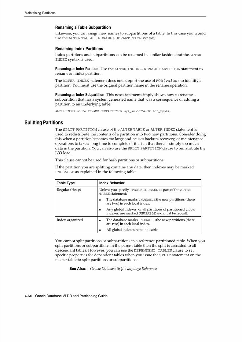
8/16/2019 Oracle Database VLDB and Partitioning Guide
http://slidepdf.com/reader/full/oracle-database-vldb-and-partitioning-guide 142/304
Maintaining Partitions
4-64 Oracle Database VLDB and Partitioning Guide
Renaming a Table Subpartition
Likewise, you can assign new names to subpartitions of a table. In this case you woulduse the ALTER TABLE ... RENAME SUBPARTITION syntax.
Renaming Index Partitions
Index partitions and subpartitions can be renamed in similar fashion, but the ALTER
INDEX syntax is used.
Renaming an Index Partition Use the ALTER INDEX ... RENAME PARTITION statement torename an index partition.
The ALTER INDEX statement does not support the use of FOR(value ) to identify apartition. You must use the original partition name in the rename operation.
Renaming an Index Subpartition This next statement simply shows how to rename asubpartition that has a system generated name that was a consequence of adding apartition to an underlying table:
ALTER INDEX scuba RENAME SUBPARTITION sys_subp3254 TO bcd_types;
Splitting PartitionsThe SPLIT PARTITION clause of the ALTER TABLE or ALTER INDEX statement isused to redistribute the contents of a partition into two new partitions. Consider doingthis when a partition becomes too large and causes backup, recovery, or maintenanceoperations to take a long time to complete or it is felt that there is simply too muchdata in the partition. You can also use the SPLIT PARTITION clause to redistribute theI/O load.
This clause cannot be used for hash partitions or subpartitions.
If the partition you are splitting contains any data, then indexes may be markedUNUSABLE as explained in the following table:
You cannot split partitions or subpartitions in a reference-partitioned table. When yousplit partitions or subpartitions in the parent table then the split is cascaded to alldescendant tables. However, you can use the DEPENDENT TABLES clause to setspecific properties for dependent tables when you issue the SPLIT statement on themaster table to split partitions or subpartitions.
Table Type Index Behavior
Regular (Heap) Unless you specify UPDATE INDEXES as part of the ALTER TABLE statement:
■ The database marks UNUSABLE the new partitions (thereare two) in each local index.
■ Any global indexes, or all partitions of partitioned globalindexes, are marked UNUSABLE and must be rebuilt.
Index-organized ■ The database marks UNUSABLE the new partitions (thereare two) in each local index.
■ All global indexes remain usable.
See Also: Oracle Database SQL Language Reference
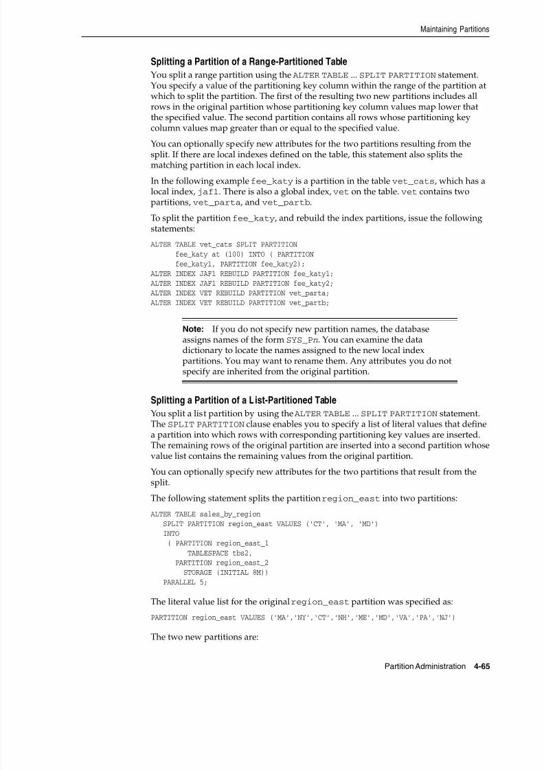
8/16/2019 Oracle Database VLDB and Partitioning Guide
http://slidepdf.com/reader/full/oracle-database-vldb-and-partitioning-guide 143/304
8/16/2019 Oracle Database VLDB and Partitioning Guide
http://slidepdf.com/reader/full/oracle-database-vldb-and-partitioning-guide 144/304
Maintaining Partitions
4-66 Oracle Database VLDB and Partitioning Guide
■ region_east_1 with a literal value list of ('CT','MA','MD')
■ region_east_2 inheriting the remaining literal value list of('NY','NH','ME','VA','PA','NJ')
The individual partitions have new physical attributes specified at the partition level.The operation is executed with parallelism of degree 5.
You can split a default list partition just like you split any other list partition. This isalso the only means of adding a partition to a list-partitioned table that contains adefault partition. When you split the default partition, you create a new partitiondefined by the values that you specify, and a second partition that remains the defaultpartition.
The following example splits the default partition of sales_by_region, therebycreating a new partition:
ALTER TABLE sales_by_regionSPLIT PARTITION region_unknown VALUES ('MT', 'WY', 'ID')INTO( PARTITION region_wildwest,
PARTITION region_unknown);
Splitting a Partition of an Interval-Partitioned Table
You split a range or a materialized interval partition using the ALTER TABLE ...SPLIT PARTITION statement in an interval-partitioned table. Splitting a rangepartition in the interval-partitioned table is described in "Splitting a Partition of aRange-Partitioned Table" on page 4-65.
To split a materialized interval partition, you specify a value of the partitioning keycolumn within the interval partition at which to split the partition. The first of theresulting two new partitions includes all rows in the original partition whosepartitioning key column values map lower than the specified value. The secondpartition contains all rows whose partitioning key column values map greater than orequal to the specified value. The split partition operation moves the transition point up
to the higher boundary of the partition you just split, and all materialized intervalpartitions lower than the newly split partitions are implicitly converted into rangepartitions, with their upper boundaries defined by the upper boundaries of theintervals.
You can optionally specify new attributes for the two range partitions resulting fromthe split. If there are local indexes defined on the table, then this statement also splitsthe matching partition in each local index. You cannot split interval partitions thathave not yet been created.
The following example shows splitting the May 2007 partition in the monthly intervalpartitioned table transactions.
ALTER TABLE transactions SPLIT PARTITION FOR(TO_DATE('01-MAY-2007','dd-MON-yyyy'))
AT (TO_DATE('15-MAY-2007','dd-MON-yyyy'));
Splitting a *-Hash Partition
This is the opposite of merging *-hash partitions. When you split *-hash partitions, thenew subpartitions are rehashed into either the number of subpartitions specified in aSUBPARTITIONS or SUBPARTITION clause. Or, if no such clause is included, the newpartitions inherit the number of subpartitions (and tablespaces) from the partition being split.
8/16/2019 Oracle Database VLDB and Partitioning Guide
http://slidepdf.com/reader/full/oracle-database-vldb-and-partitioning-guide 145/304
Maintaining Partitions
Partition Administration 4-67
Note that the inheritance of properties is different when a *-hash partition is split,versus when two *-hash partitions are merged. When a partition is split, the newpartitions can inherit properties from the original partition because there is only oneparent. However, when partitions are merged, properties must be inherited from tablelevel defaults because there are two parents and the new partition cannot inherit fromeither at the expense of the other.
The following example splits a range-hash partition:ALTER TABLE all_seasons SPLIT PARTITION quarter_1
AT (TO_DATE('16-dec-1997','dd-mon-yyyy')) INTO (PARTITION q1_1997_1 SUBPARTITIONS 4 STORE IN (ts1,ts3), PARTITION q1_1997_2);
The rules for splitting an interval-hash partitioned table follow the rules for splittingan interval-partitioned table. As described in "Splitting a Partition of anInterval-Partitioned Table" on page 4-66, the transition point is changed to the higher boundary of the split partition.
Splitting Partitions in a *-List Partitioned Table
Partitions can be split at both the partition level and at the list subpartition level.
Splitting a *-List Partition Splitting a partition of a *-list partitioned table is similar to thedescription in "Splitting a Partition of a Range-Partitioned Table" on page 4-65. Nosubpartition literal value list can be specified for either of the new partitions. The newpartitions inherit the subpartition descriptions from the original partition being split.
The following example splits the q1_1999 partition of the quarterly_regional_sales table:
ALTER TABLE quarterly_regional_sales SPLIT PARTITION q1_1999 AT (TO_DATE('15-Feb-1999','dd-mon-yyyy')) INTO ( PARTITION q1_1999_jan_feb TABLESPACE ts1, PARTITION q1_1999_feb_mar
STORAGE (INITIAL 8M) TABLESPACE ts2)PARALLEL 5;
This operation splits the partition q1_1999 into two resulting partitions: q1_1999_jan_feb and q1_1999_feb_mar. Both partitions inherit their subpartitiondescriptions from the original partition. The individual partitions have new physicalattributes, including tablespaces, specified at the partition level. These new attributes become the default attributes of the new partitions. This operation is run withparallelism of degree 5.
The ALTER TABLE ... SPLIT PARTITION statement provides no means of specificallynaming subpartitions resulting from the split of a partition in a composite partitionedtable. However, for those subpartitions in the parent partition with names of the form
partition name_subpartition name , the database generates correspondingnames in the newly created subpartitions using the new partition names. All othersubpartitions are assigned system generated names of the form SYS_SUBPn. Systemgenerated names are also assigned for the subpartitions of any partition resulting fromthe split for which a name is not specified. Unnamed partitions are assigned a systemgenerated partition name of the form SYS_Pn.
The following query displays the subpartition names resulting from the previous splitpartition operation on table quarterly_regional_sales. It also reflects the resultsof other operations performed on this table in preceding sections of this chapter sinceits creation in "Creating Composite Range-List Partitioned Tables" on page 4-10.
8/16/2019 Oracle Database VLDB and Partitioning Guide
http://slidepdf.com/reader/full/oracle-database-vldb-and-partitioning-guide 146/304
Maintaining Partitions
4-68 Oracle Database VLDB and Partitioning Guide
SELECT PARTITION_NAME, SUBPARTITION_NAME, TABLESPACE_NAME FROM DBA_TAB_SUBPARTITIONS WHERE TABLE_NAME='QUARTERLY_REGIONAL_SALES' ORDER BY PARTITION_NAME;
PARTITION_NAME SUBPARTITION_NAME TABLESPACE_NAME-------------------- ------------------------------ ---------------Q1_1999_FEB_MAR Q1_1999_FEB_MAR_WEST TS2Q1_1999_FEB_MAR Q1_1999_FEB_MAR_NORTHEAST TS2Q1_1999_FEB_MAR Q1_1999_FEB_MAR_SOUTHEAST TS2Q1_1999_FEB_MAR Q1_1999_FEB_MAR_NORTHCENTRAL TS2Q1_1999_FEB_MAR Q1_1999_FEB_MAR_SOUTHCENTRAL TS2Q1_1999_FEB_MAR Q1_1999_FEB_MAR_SOUTH TS2Q1_1999_JAN_FEB Q1_1999_JAN_FEB_WEST TS1Q1_1999_JAN_FEB Q1_1999_JAN_FEB_NORTHEAST TS1Q1_1999_JAN_FEB Q1_1999_JAN_FEB_SOUTHEAST TS1Q1_1999_JAN_FEB Q1_1999_JAN_FEB_NORTHCENTRAL TS1Q1_1999_JAN_FEB Q1_1999_JAN_FEB_SOUTHCENTRAL TS1Q1_1999_JAN_FEB Q1_1999_JAN_FEB_SOUTH TS1Q1_2000 Q1_2000_NORTHWEST TS3Q1_2000 Q1_2000_SOUTHWEST TS3Q1_2000 Q1_2000_NORTHEAST TS3Q1_2000 Q1_2000_SOUTHEAST TS3Q1_2000 Q1_2000_NORTHCENTRAL TS3Q1_2000 Q1_2000_SOUTHCENTRAL TS3Q2_1999 Q2_1999_NORTHWEST TS4Q2_1999 Q2_1999_SOUTHWEST TS4Q2_1999 Q2_1999_NORTHEAST TS4Q2_1999 Q2_1999_SOUTHEAST TS4Q2_1999 Q2_1999_NORTHCENTRAL TS4Q2_1999 Q2_1999_SOUTHCENTRAL TS4Q3_1999 Q3_1999_NORTHWEST TS4Q3_1999 Q3_1999_SOUTHWEST TS4Q3_1999 Q3_1999_NORTHEAST TS4Q3_1999 Q3_1999_SOUTHEAST TS4
Q3_1999 Q3_1999_NORTHCENTRAL TS4Q3_1999 Q3_1999_SOUTHCENTRAL TS4Q4_1999 Q4_1999_NORTHWEST TS4Q4_1999 Q4_1999_SOUTHWEST TS4Q4_1999 Q4_1999_NORTHEAST TS4Q4_1999 Q4_1999_SOUTHEAST TS4Q4_1999 Q4_1999_NORTHCENTRAL TS4Q4_1999 Q4_1999_SOUTHCENTRAL TS4
36 rows selected.
Splitting a *-List Subpartition Splitting a list subpartition of a *-list partitioned table issimilar to the description in "Splitting a Partition of a List-Partitioned Table" onpage 4-65, but the syntax is that of SUBPARTITION rather than PARTITION. For
example, the following statement splits a subpartition of the quarterly_regional_sales table:
ALTER TABLE quarterly_regional_sales SPLIT SUBPARTITION q2_1999_southwest VALUES ('UT') INTO ( SUBPARTITION q2_1999_utah TABLESPACE ts2, SUBPARTITION q2_1999_southwest TABLESPACE ts3 )
PARALLEL;
8/16/2019 Oracle Database VLDB and Partitioning Guide
http://slidepdf.com/reader/full/oracle-database-vldb-and-partitioning-guide 147/304
Maintaining Partitions
Partition Administration 4-69
This operation splits the subpartition q2_1999_southwest into two subpartitions:
■ q2_1999_utah with literal value list of ('UT')
■ q2_1999_southwest which inherits the remaining literal value list of('AZ','NM')
The individual subpartitions have new physical attributes that are inherited from thesubpartition being split.
You can only split subpartitions in an interval-list partitioned table for range partitionsor materialized interval partitions. To change subpartition values for future intervalpartitions, you must modify the subpartition template.
Splitting a *-Range Partition
Splitting a partition of a *-range partitioned table is similar to the description in"Splitting a Partition of a Range-Partitioned Table" on page 4-65. No subpartition rangevalues can be specified for either of the new partitions. The new partitions inherit thesubpartition descriptions from the original partition being split.
The following example splits the May 2007 interval partition of the interval-range
partitioned orders table:
ALTER TABLE orders SPLIT PARTITION FOR(TO_DATE('01-MAY-2007','dd-MON-yyyy')) AT (TO_DATE('15-MAY-2007','dd-MON-yyyy')) INTO (PARTITION p_fh_may07,PARTITION p_sh_may2007);
This operation splits the interval partition FOR('01-MAY-2007') into two resultingpartitions: p_fh_may07 and p_sh_may_2007. Both partitions inherit theirsubpartition descriptions from the original partition. Any interval partitions before the June 2007 partition have been converted into range partitions, as described in"Merging Interval Partitions" on page 4-51.
The ALTER TABLE ... SPLIT PARTITION statement provides no means of
specifically naming subpartitions resulting from the split of a partition in a compositepartitioned table. However, for those subpartitions in the parent partition with namesof the form partition name _subpartition name , the database generatescorresponding names in the newly created subpartitions using the new partitionnames. All other subpartitions are assigned system generated names of the form SYS_SUBPn. System generated names are also assigned for the subpartitions of anypartition resulting from the split for which a name is not specified. Unnamedpartitions are assigned a system generated partition name of the form SYS_Pn.
The following query displays the subpartition names and high values resulting fromthe previous split partition operation on table orders. It also reflects the results ofother operations performed on this table in preceding sections of this chapter since itscreation.
BREAK ON partition_name
SELECT partition_name, subpartition_name, high_valueFROM user_tab_subpartitions
WHERE table_name = 'ORCERS'ORDER BY partition_name, subpartition_position;
PARTITION_NAME SUBPARTITION_NAME HIGH_VALUE------------------------- ------------------------------ ---------------P_BEFORE_2007 P_BEFORE_2007_P_SMALL 1000 P_BEFORE_2007_P_MEDIUM 10000
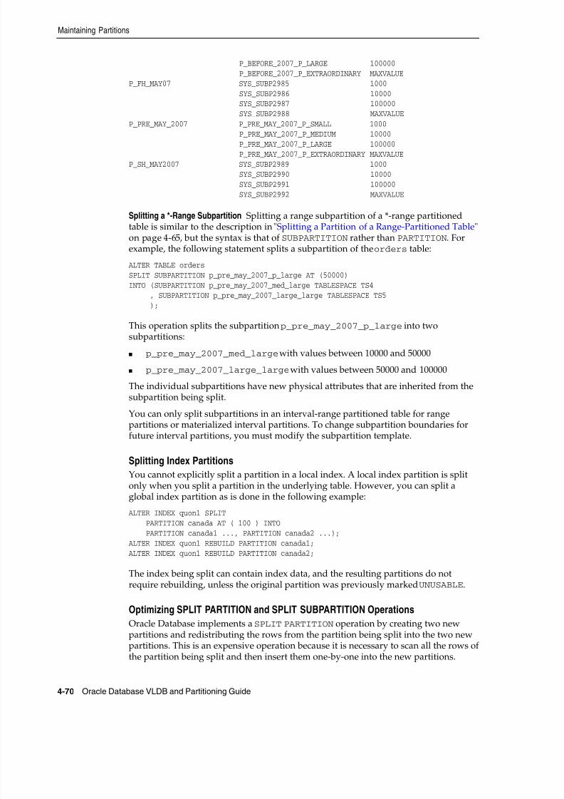
8/16/2019 Oracle Database VLDB and Partitioning Guide
http://slidepdf.com/reader/full/oracle-database-vldb-and-partitioning-guide 148/304

8/16/2019 Oracle Database VLDB and Partitioning Guide
http://slidepdf.com/reader/full/oracle-database-vldb-and-partitioning-guide 149/304
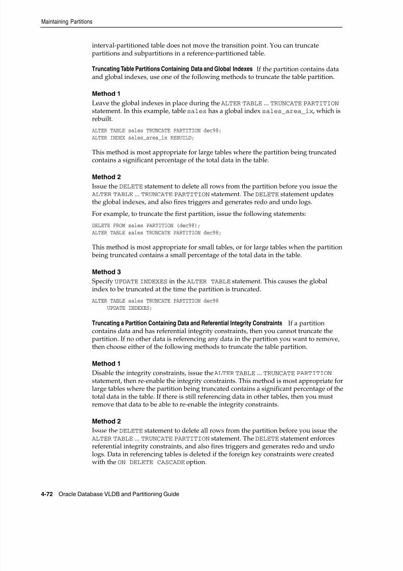
8/16/2019 Oracle Database VLDB and Partitioning Guide
http://slidepdf.com/reader/full/oracle-database-vldb-and-partitioning-guide 150/304
Maintaining Partitions
4-72 Oracle Database VLDB and Partitioning Guide
interval-partitioned table does not move the transition point. You can truncatepartitions and subpartitions in a reference-partitioned table.
Truncating Table Partitions Containing Data and Global Indexes If the partition contains dataand global indexes, use one of the following methods to truncate the table partition.
Method 1
Leave the global indexes in place during the ALTER TABLE ... TRUNCATE PARTITION statement. In this example, table sales has a global index sales_area_ix, which isrebuilt.
ALTER TABLE sales TRUNCATE PARTITION dec98;ALTER INDEX sales_area_ix REBUILD;
This method is most appropriate for large tables where the partition being truncatedcontains a significant percentage of the total data in the table.
Method 2
Issue the DELETE statement to delete all rows from the partition before you issue theALTER TABLE ... TRUNCATE PARTITION statement. The DELETE statement updates
the global indexes, and also fires triggers and generates redo and undo logs.
For example, to truncate the first partition, issue the following statements:
DELETE FROM sales PARTITION (dec98);ALTER TABLE sales TRUNCATE PARTITION dec98;
This method is most appropriate for small tables, or for large tables when the partition being truncated contains a small percentage of the total data in the table.
Method 3
Specify UPDATE INDEXES in the ALTER TABLE statement. This causes the globalindex to be truncated at the time the partition is truncated.
ALTER TABLE sales TRUNCATE PARTITION dec98 UPDATE INDEXES;
Truncating a Partition Containing Data and Referential Integrity Constraints If a partitioncontains data and has referential integrity constraints, then you cannot truncate thepartition. If no other data is referencing any data in the partition you want to remove,then choose either of the following methods to truncate the table partition.
Method 1
Disable the integrity constraints, issue the ALTER TABLE ... TRUNCATE PARTITION statement, then re-enable the integrity constraints. This method is most appropriate forlarge tables where the partition being truncated contains a significant percentage of the
total data in the table. If there is still referencing data in other tables, then you mustremove that data to be able to re-enable the integrity constraints.
Method 2
Issue the DELETE statement to delete all rows from the partition before you issue theALTER TABLE ... TRUNCATE PARTITION statement. The DELETE statement enforcesreferential integrity constraints, and also fires triggers and generates redo and undologs. Data in referencing tables is deleted if the foreign key constraints were createdwith the ON DELETE CASCADE option.
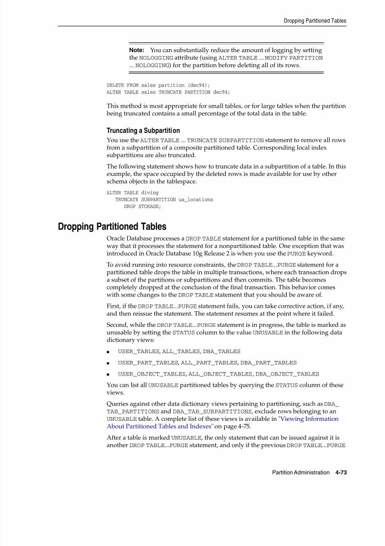
8/16/2019 Oracle Database VLDB and Partitioning Guide
http://slidepdf.com/reader/full/oracle-database-vldb-and-partitioning-guide 151/304
Dropping Partitioned Tables
Partition Administration 4-73
DELETE FROM sales partition (dec94);ALTER TABLE sales TRUNCATE PARTITION dec94;
This method is most appropriate for small tables, or for large tables when the partition being truncated contains a small percentage of the total data in the table.
Truncating a Subpartition
You use the ALTER TABLE ... TRUNCATE SUBPARTITION statement to remove all rowsfrom a subpartition of a composite partitioned table. Corresponding local indexsubpartitions are also truncated.
The following statement shows how to truncate data in a subpartition of a table. In thisexample, the space occupied by the deleted rows is made available for use by otherschema objects in the tablespace.
ALTER TABLE diving TRUNCATE SUBPARTITION us_locations DROP STORAGE;
Dropping Partitioned TablesOracle Database processes a DROP TABLE statement for a partitioned table in the sameway that it processes the statement for a nonpartitioned table. One exception that wasintroduced in Oracle Database 10g Release 2 is when you use the PURGE keyword.
To avoid running into resource constraints, the DROP TABLE...PURGE statement for apartitioned table drops the table in multiple transactions, where each transaction dropsa subset of the partitions or subpartitions and then commits. The table becomes
completely dropped at the conclusion of the final transaction. This behavior comeswith some changes to the DROP TABLE statement that you should be aware of.
First, if the DROP TABLE...PURGE statement fails, you can take corrective action, if any,and then reissue the statement. The statement resumes at the point where it failed.
Second, while the DROP TABLE...PURGE statement is in progress, the table is marked asunusable by setting the STATUS column to the value UNUSABLE in the following datadictionary views:
■ USER_TABLES, ALL_TABLES, DBA_TABLES
■ USER_PART_TABLES, ALL_PART_TABLES, DBA_PART_TABLES
■ USER_OBJECT_TABLES, ALL_OBJECT_TABLES, DBA_OBJECT_TABLES
You can list all UNUSABLE partitioned tables by querying the STATUS column of theseviews.
Queries against other data dictionary views pertaining to partitioning, such as DBA_TAB_PARTITIONS and DBA_TAB_SUBPARTITIONS, exclude rows belonging to anUNUSABLE table. A complete list of these views is available in "Viewing InformationAbout Partitioned Tables and Indexes" on page 4-75.
After a table is marked UNUSABLE, the only statement that can be issued against it isanother DROP TABLE...PURGE statement, and only if the previous DROP TABLE...PURGE
Note: You can substantially reduce the amount of logging by settingthe NOLOGGING attribute (using ALTER TABLE ... MODIFY PARTITION ... NOLOGGING) for the partition before deleting all of its rows.
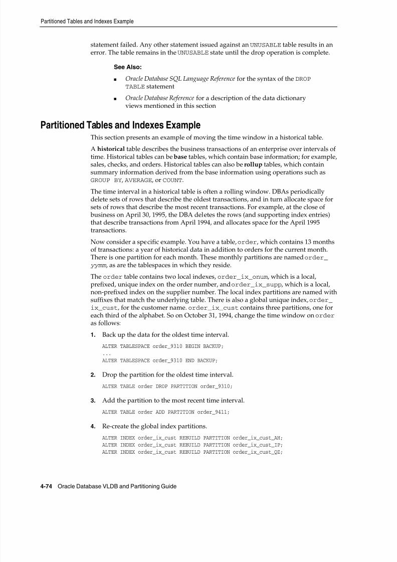
8/16/2019 Oracle Database VLDB and Partitioning Guide
http://slidepdf.com/reader/full/oracle-database-vldb-and-partitioning-guide 152/304
Partitioned Tables and Indexes Example
4-74 Oracle Database VLDB and Partitioning Guide
statement failed. Any other statement issued against an UNUSABLE table results in anerror. The table remains in the UNUSABLE state until the drop operation is complete.
Partitioned Tables and Indexes ExampleThis section presents an example of moving the time window in a historical table.
A historical table describes the business transactions of an enterprise over intervals oftime. Historical tables can be base tables, which contain base information; for example,sales, checks, and orders. Historical tables can also be rollup tables, which containsummary information derived from the base information using operations such asGROUP BY, AVERAGE, or COUNT.
The time interval in a historical table is often a rolling window. DBAs periodicallydelete sets of rows that describe the oldest transactions, and in turn allocate space forsets of rows that describe the most recent transactions. For example, at the close of business on April 30, 1995, the DBA deletes the rows (and supporting index entries)that describe transactions from April 1994, and allocates space for the April 1995transactions.
Now consider a specific example. You have a table, order, which contains 13 monthsof transactions: a year of historical data in addition to orders for the current month.There is one partition for each month. These monthly partitions are named order_ yymm , as are the tablespaces in which they reside.
The order table contains two local indexes, order_ix_onum , which is a local,prefixed, unique index on the order number, and order_ix_supp, which is a local,
non-prefixed index on the supplier number. The local index partitions are named withsuffixes that match the underlying table. There is also a global unique index, order_ix_cust, for the customer name. order_ix_cust contains three partitions, one foreach third of the alphabet. So on October 31, 1994, change the time window on order as follows:
1. Back up the data for the oldest time interval.
ALTER TABLESPACE order_9310 BEGIN BACKUP;...ALTER TABLESPACE order_9310 END BACKUP;
2. Drop the partition for the oldest time interval.
ALTER TABLE order DROP PARTITION order_9310;
3. Add the partition to the most recent time interval.
ALTER TABLE order ADD PARTITION order_9411;
4. Re-create the global index partitions.
ALTER INDEX order_ix_cust REBUILD PARTITION order_ix_cust_AH;ALTER INDEX order_ix_cust REBUILD PARTITION order_ix_cust_IP;ALTER INDEX order_ix_cust REBUILD PARTITION order_ix_cust_QZ;
See Also:
■ Oracle Database SQL Language Reference for the syntax of the DROPTABLE statement
■ Oracle Database Reference for a description of the data dictionaryviews mentioned in this section
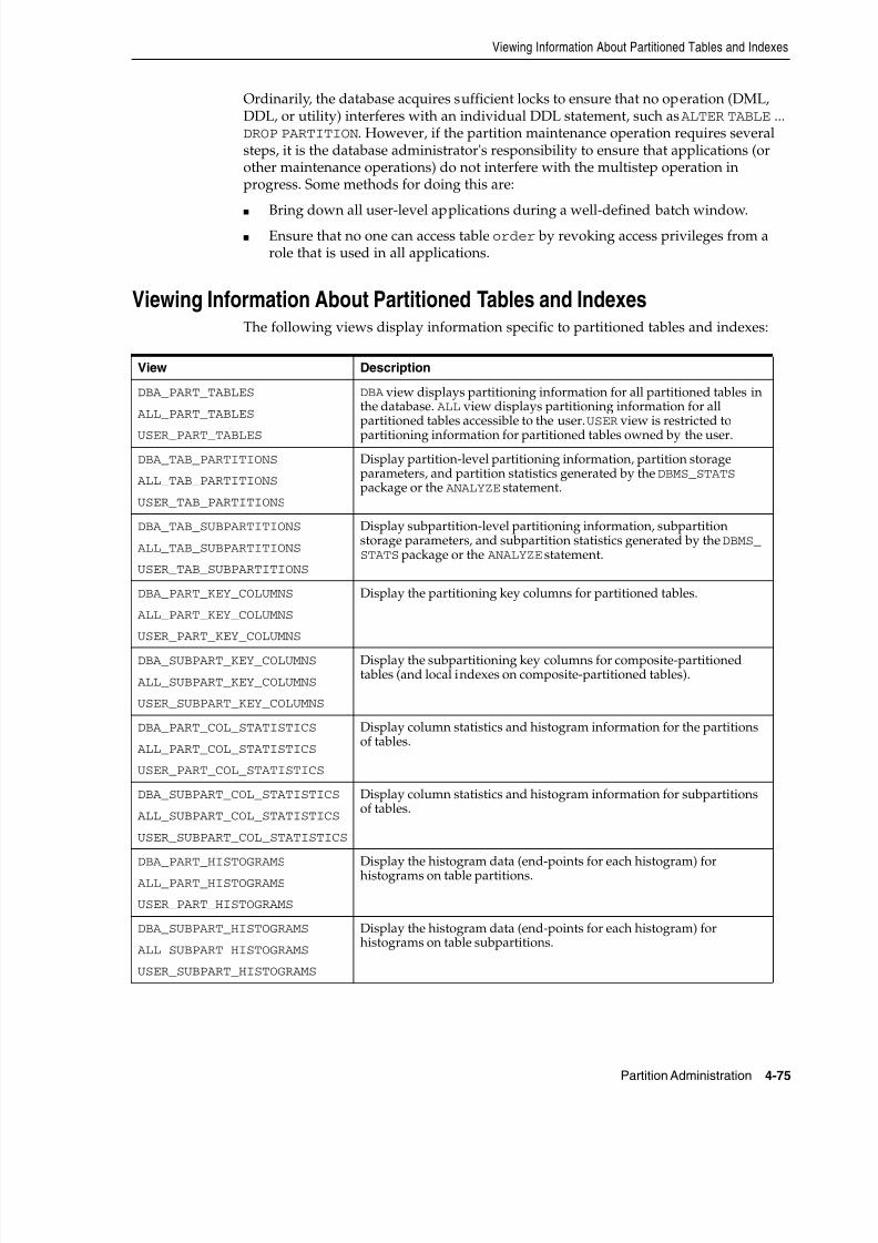
8/16/2019 Oracle Database VLDB and Partitioning Guide
http://slidepdf.com/reader/full/oracle-database-vldb-and-partitioning-guide 153/304
Viewing Information About Partitioned Tables and Indexes
Partition Administration 4-75
Ordinarily, the database acquires sufficient locks to ensure that no operation (DML,DDL, or utility) interferes with an individual DDL statement, such as ALTER TABLE ...DROP PARTITION. However, if the partition maintenance operation requires severalsteps, it is the database administrator's responsibility to ensure that applications (orother maintenance operations) do not interfere with the multistep operation inprogress. Some methods for doing this are:
■
Bring down all user-level applications during a well-defined batch window.■ Ensure that no one can access table order by revoking access privileges from a
role that is used in all applications.
Viewing Information About Partitioned Tables and IndexesThe following views display information specific to partitioned tables and indexes:
View Description
DBA_PART_TABLES
ALL_PART_TABLES
USER_PART_TABLES
DBA view displays partitioning information for all partitioned tables inthe database. ALL view displays partitioning information for allpartitioned tables accessible to the user.USER view is restricted to
partitioning information for partitioned tables owned by the user.
DBA_TAB_PARTITIONS
ALL_TAB_PARTITIONS
USER_TAB_PARTITIONS
Display partition-level partitioning information, partition storageparameters, and partition statistics generated by the DBMS_STATS package or the ANALYZE statement.
DBA_TAB_SUBPARTITIONS
ALL_TAB_SUBPARTITIONS
USER_TAB_SUBPARTITIONS
Display subpartition-level partitioning information, subpartitionstorage parameters, and subpartition statistics generated by the DBMS_STATS package or the ANALYZE statement.
DBA_PART_KEY_COLUMNS
ALL_PART_KEY_COLUMNS
USER_PART_KEY_COLUMNS
Display the partitioning key columns for partitioned tables.
DBA_SUBPART_KEY_COLUMNS
ALL_SUBPART_KEY_COLUMNS
USER_SUBPART_KEY_COLUMNS
Display the subpartitioning key columns for composite-partitionedtables (and local indexes on composite-partitioned tables).
DBA_PART_COL_STATISTICS
ALL_PART_COL_STATISTICS
USER_PART_COL_STATISTICS
Display column statistics and histogram information for the partitionsof tables.
DBA_SUBPART_COL_STATISTICS
ALL_SUBPART_COL_STATISTICS
USER_SUBPART_COL_STATISTICS
Display column statistics and histogram information for subpartitionsof tables.
DBA_PART_HISTOGRAMS
ALL_PART_HISTOGRAMS
USER_PART_HISTOGRAMS
Display the histogram data (end-points for each histogram) forhistograms on table partitions.
DBA_SUBPART_HISTOGRAMS
ALL_SUBPART_HISTOGRAMS
USER_SUBPART_HISTOGRAMS
Display the histogram data (end-points for each histogram) forhistograms on table subpartitions.

8/16/2019 Oracle Database VLDB and Partitioning Guide
http://slidepdf.com/reader/full/oracle-database-vldb-and-partitioning-guide 154/304
Viewing Information About Partitioned Tables and Indexes
4-76 Oracle Database VLDB and Partitioning Guide
DBA_PART_INDEXES
ALL_PART_INDEXES
USER_PART_INDEXES
Display partitioning information for partitioned indexes.
DBA_IND_PARTITIONS
ALL_IND_PARTITIONS
USER_IND_PARTITIONS
Display the following for index partitions: partition-level partitioning
information, storage parameters for the partition, statistics collected bythe DBMS_STATS package or the ANALYZE statement.
DBA_IND_SUBPARTITIONS
ALL_IND_SUBPARTITIONS
USER_IND_SUBPARTITIONS
Display the following information for index subpartitions:partition-level partitioning information, storage parameters for thepartition, statistics collected by the DBMS_STATS package or theANALYZE statement.
DBA_SUBPARTITION_TEMPLATES
ALL_SUBPARTITION_TEMPLATES
USER_SUBPARTITION_TEMPLATES
Display information about existing subpartition templates.
See Also:
■ Oracle Database Reference for complete descriptions of these views
■ Oracle Database Performance Tuning Guide and Oracle DatabasePerformance Tuning Guide for information about histograms andgenerating statistics for tables
■ Oracle Database Administrator's Guide for more information aboutanalyzing tables, indexes, and clusters
View Description
8/16/2019 Oracle Database VLDB and Partitioning Guide
http://slidepdf.com/reader/full/oracle-database-vldb-and-partitioning-guide 155/304
5
Using Partitioning for Information Lifecycle Management 5-1
5Using Partitioning for Information LifecycleManagement
This chapter discusses the components in Oracle Database which can build anInformation Lifecycle Management (ILM) strategy to manage and maintain data.
Although most organizations have long regarded their stores of data as one of theirmost valuable corporate assets, how this data was managed and maintained varies
enormously. Originally, data was used to help achieve operational goals, run the business, and help identify the future direction and success of the company.
However, new government regulations and guidelines are a key driving force in howand why data is being retained, as they are now requiring organizations to retain andcontrol information for very long periods of time. Consequently, today there are twoadditional objectives IT managers are trying to satisfy: to store vast quantities of data,for the lowest possible cost; and to meet the new regulatory requirements for dataretention and protection.
This chapter contains the following topics:
■ What Is ILM?
■
Implementing ILM Using Oracle Database■ The Benefits of an Online Archive
■ Oracle ILM Assistant
■ Implementing an ILM System Manually
What Is ILM?Information today comes in a wide variety of types, for example an E-mail message, aphotograph, or an order in an Online Transaction Processing System. After you knowthe type of data and how it is used, you have an understanding of what its evolutionand final destiny is likely to be.
One challenge facing each organization is to understand how its data evolves andgrows, monitor how its usage changes over time, and decide how long it shouldsurvive, while adhering to all the rules and regulations that now apply to that data.Information Lifecycle Management (ILM) is designed to address these issues, with acombination of processes, policies, software, and hardware so that the appropriatetechnology can be used for each stage in the lifecycle of the data.
8/16/2019 Oracle Database VLDB and Partitioning Guide
http://slidepdf.com/reader/full/oracle-database-vldb-and-partitioning-guide 156/304
8/16/2019 Oracle Database VLDB and Partitioning Guide
http://slidepdf.com/reader/full/oracle-database-vldb-and-partitioning-guide 157/304
Implementing ILM Using Oracle Database
Using Partitioning for Information Lifecycle Management 5-3
These regulations frequently demand that electronic data is secure from unauthorizedaccess and changes, and that there is an audit trail of all changes to data and by whom.Oracle Database can retain huge quantities of data without impacting applicationperformance. It also contains the features required to restrict access and preventunauthorized changes to data, and can be further enhanced with Oracle DatabaseVault and Oracle Audit Vault. Oracle Database also provides cryptographic functionsthat can demonstrate that a highly privileged user has not intentionally modified data.
Flashback Data Archive can show all the versions of a row during its lifetime.
Implementing ILM Using Oracle DatabaseBuilding an Information Lifecycle Management solution using Oracle Database isquite straightforward and can be completed by following these four simple steps,although Step 4 is optional if ILM is not being implemented for compliance:
■ Step 1: Define the Data Classes
■ Step 2: Create Storage Tiers for the Data Classes
■ Step 3: Create Data Access and Migration Policies
■
Step 4: Define and Enforce Compliance Policies
Step 1: Define the Data ClassesTo make effective use of Information Lifecycle Management, the first step is to look atall the data in your organization and determine:
■ What data is important, where is it stored, and what must be retained
■ How this data flows within the organization
■ What happens to this data over time and whether it is still needed
■ The degree of data availability and protection that is needed
■ Data retention for legal and business requirements
After there is an understanding of how the data is used, it can then be classified on this basis. The most common type of classification is by age or date, but other types arepossible, such as by product or privacy. A hybrid classification could also be used,such as by privacy and age.
To treat the data classes differently, the data must be physically separated. Wheninformation is first created, it is often frequently accessed, but then over time it may bereferenced very infrequently. For instance, when a customer places an order, theyregularly look at the order to see its status and whether it has been shipped. After itarrives, they may never reference that order again. This order would also be includedin regular reports that are run to see what goods are being ordered, but, over time,would not figure in any of the reports and may only be referenced in the future if
someone does a detailed analysis that involves this data. Therefore, orders could beclassified by the Financial Quarters Q1, Q2, Q3, and Q4, and as Historical Orders.
The advantage of using this approach is that when the data is grouped at the row level by its class, which in this example would be the date of the order, all orders for Q1 can be managed as a self contained unit, where as the orders for Q2 would reside in adifferent class. This can be achieved by using partitioning. Because partitions arecompletely transparent to the application, the data is physically separated but theapplication still sees all of the orders.
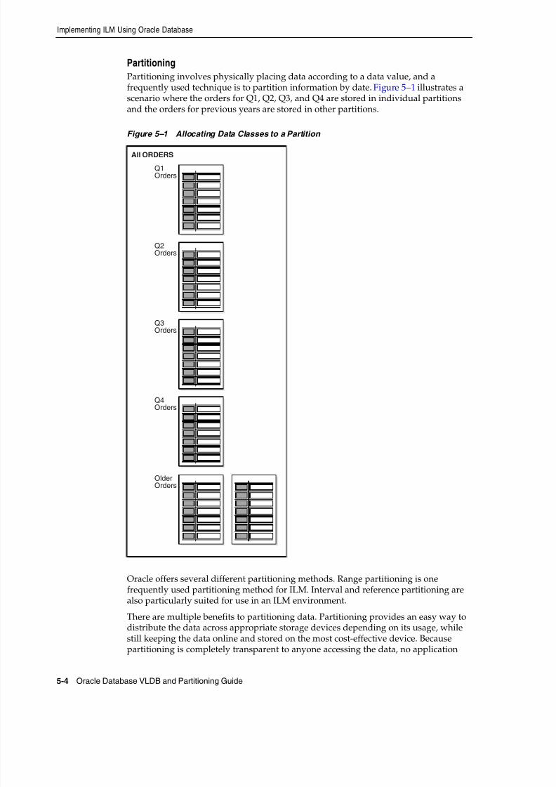
8/16/2019 Oracle Database VLDB and Partitioning Guide
http://slidepdf.com/reader/full/oracle-database-vldb-and-partitioning-guide 158/304
Implementing ILM Using Oracle Database
5-4 Oracle Database VLDB and Partitioning Guide
Partitioning
Partitioning involves physically placing data according to a data value, and afrequently used technique is to partition information by date. Figure 5–1 illustrates ascenario where the orders for Q1, Q2, Q3, and Q4 are stored in individual partitionsand the orders for previous years are stored in other partitions.
Figure 5–1 Allocating Data Classes to a Partition
Oracle offers several different partitioning methods. Range partitioning is onefrequently used partitioning method for ILM. Interval and reference partitioning arealso particularly suited for use in an ILM environment.
There are multiple benefits to partitioning data. Partitioning provides an easy way todistribute the data across appropriate storage devices depending on its usage, whilestill keeping the data online and stored on the most cost-effective device. Becausepartitioning is completely transparent to anyone accessing the data, no application
All ORDERS
Q1Orders
Q2Orders
Q3Orders
Q4Orders
OlderOrders
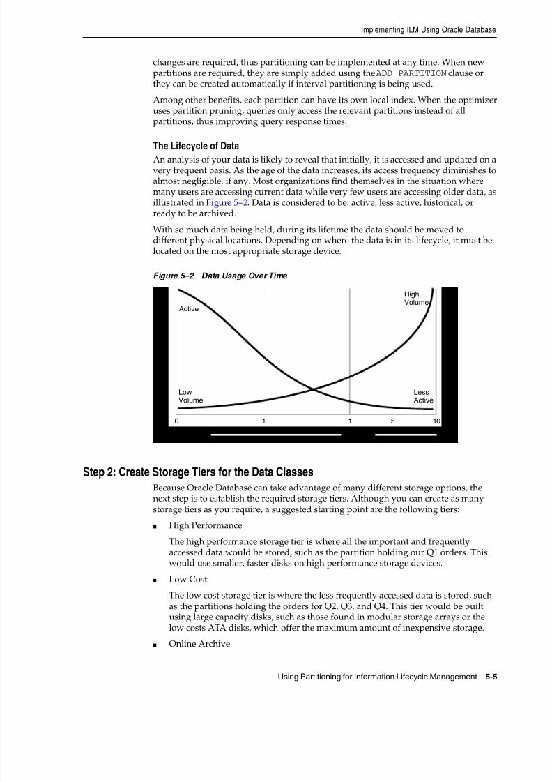
8/16/2019 Oracle Database VLDB and Partitioning Guide
http://slidepdf.com/reader/full/oracle-database-vldb-and-partitioning-guide 159/304
Implementing ILM Using Oracle Database
Using Partitioning for Information Lifecycle Management 5-5
changes are required, thus partitioning can be implemented at any time. When newpartitions are required, they are simply added using the ADD PARTITION clause orthey can be created automatically if interval partitioning is being used.
Among other benefits, each partition can have its own local index. When the optimizeruses partition pruning, queries only access the relevant partitions instead of allpartitions, thus improving query response times.
The Lifecycle of Data
An analysis of your data is likely to reveal that initially, it is accessed and updated on avery frequent basis. As the age of the data increases, its access frequency diminishes toalmost negligible, if any. Most organizations find themselves in the situation wheremany users are accessing current data while very few users are accessing older data, asillustrated in Figure 5–2. Data is considered to be: active, less active, historical, orready to be archived.
With so much data being held, during its lifetime the data should be moved todifferent physical locations. Depending on where the data is in its lifecycle, it must belocated on the most appropriate storage device.
Figure 5–2 Data Usage Over Time
Step 2: Create Storage Tiers for the Data ClassesBecause Oracle Database can take advantage of many different storage options, thenext step is to establish the required storage tiers. Although you can create as manystorage tiers as you require, a suggested starting point are the following tiers:
■ High Performance
The high performance storage tier is where all the important and frequentlyaccessed data would be stored, such as the partition holding our Q1 orders. Thiswould use smaller, faster disks on high performance storage devices.
■ Low Cost
The low cost storage tier is where the less frequently accessed data is stored, suchas the partitions holding the orders for Q2, Q3, and Q4. This tier would be builtusing large capacity disks, such as those found in modular storage arrays or thelow costs ATA disks, which offer the maximum amount of inexpensive storage.
■ Online Archive
Months Years
A c
t i v i t y
D a
t a V o l u m e
0 1 1 5 10
Active
HighVolume
LessActive
LowVolume
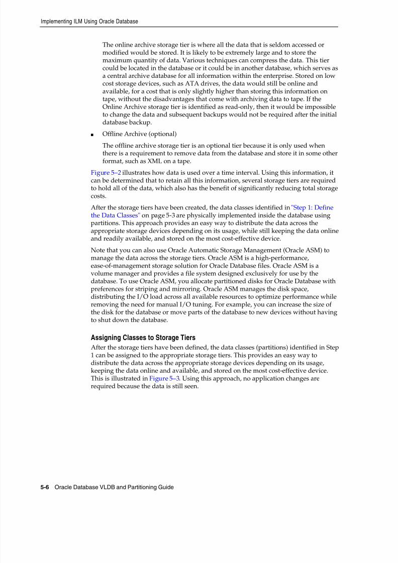
8/16/2019 Oracle Database VLDB and Partitioning Guide
http://slidepdf.com/reader/full/oracle-database-vldb-and-partitioning-guide 160/304
Implementing ILM Using Oracle Database
5-6 Oracle Database VLDB and Partitioning Guide
The online archive storage tier is where all the data that is seldom accessed ormodified would be stored. It is likely to be extremely large and to store themaximum quantity of data. Various techniques can compress the data. This tiercould be located in the database or it could be in another database, which serves asa central archive database for all information within the enterprise. Stored on lowcost storage devices, such as ATA drives, the data would still be online andavailable, for a cost that is only slightly higher than storing this information on
tape, without the disadvantages that come with archiving data to tape. If theOnline Archive storage tier is identified as read-only, then it would be impossibleto change the data and subsequent backups would not be required after the initialdatabase backup.
■ Offline Archive (optional)
The offline archive storage tier is an optional tier because it is only used whenthere is a requirement to remove data from the database and store it in some otherformat, such as XML on a tape.
Figure 5–2 illustrates how data is used over a time interval. Using this information, itcan be determined that to retain all this information, several storage tiers are requiredto hold all of the data, which also has the benefit of significantly reducing total storage
costs.After the storage tiers have been created, the data classes identified in "Step 1: Definethe Data Classes" on page 5-3 are physically implemented inside the database usingpartitions. This approach provides an easy way to distribute the data across theappropriate storage devices depending on its usage, while still keeping the data onlineand readily available, and stored on the most cost-effective device.
Note that you can also use Oracle Automatic Storage Management (Oracle ASM) tomanage the data across the storage tiers. Oracle ASM is a high-performance,ease-of-management storage solution for Oracle Database files. Oracle ASM is avolume manager and provides a file system designed exclusively for use by thedatabase. To use Oracle ASM, you allocate partitioned disks for Oracle Database withpreferences for striping and mirroring. Oracle ASM manages the disk space,
distributing the I/O load across all available resources to optimize performance whileremoving the need for manual I/O tuning. For example, you can increase the size ofthe disk for the database or move parts of the database to new devices without havingto shut down the database.
Assigning Classes to Storage Tiers
After the storage tiers have been defined, the data classes (partitions) identified in Step1 can be assigned to the appropriate storage tiers. This provides an easy way todistribute the data across the appropriate storage devices depending on its usage,keeping the data online and available, and stored on the most cost-effective device.This is illustrated in Figure 5–3. Using this approach, no application changes arerequired because the data is still seen.
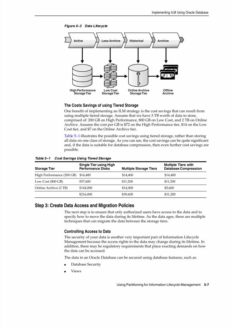
8/16/2019 Oracle Database VLDB and Partitioning Guide
http://slidepdf.com/reader/full/oracle-database-vldb-and-partitioning-guide 161/304
8/16/2019 Oracle Database VLDB and Partitioning Guide
http://slidepdf.com/reader/full/oracle-database-vldb-and-partitioning-guide 162/304
Implementing ILM Using Oracle Database
5-8 Oracle Database VLDB and Partitioning Guide
■ Virtual Private Database
Virtual Private Database (VPD) defines a very fine-grained level of access to thedatabase. Security policies determine which rows may be viewed and the columns thatare visible. Multiple policies can be defined so that different users and applications seedifferent views of the same data. For example, the majority of users could see theinformation for Q1, Q2, Q3, and Q4, while only authorized users would be able to
view the historical data.A security policy is defined at the database level and is transparently applied to alldatabase users. The benefit of this approach is that it provides a secure and controlledenvironment for accessing the data, which cannot be overridden and can beimplemented without requiring any application changes. In addition, read-onlytablespaces can be defined which ensures that the data does not change.
Moving Data using Partitioning
During its lifetime, data must be moved. This may occur for the following reasons:
■ For performance, only a limited number of orders are held on high performancedisks
■ Data is no longer frequently accessed and is using valuable high performancestorage, and must be moved to a low-cost storage device
■ Legal requirements demand that the information is always available for a giventime interval, and it must be held safely for the lowest possible cost
There are multiple ways that data can be physically moved in Oracle Database to takeadvantage of the different storage tiers. For example, if the data is partitioned, then apartition containing the orders for Q2 could be moved online from the highperformance storage tier to the low cost storage tier. Because the data is being movedwithin the database, it can be physically moved, without affecting the applications thatrequire it or causing disruption to regular users.
Sometimes individual data items, rather than a group of data, must be moved. For
example, suppose data was classified according to a level of privacy and a report,which had been secret, is now to be made available to the public. If the classificationchanged from secret to public and the data was partitioned on its privacyclassification, then the row would automatically move to the partition containingpublic data.
Whenever data is moved from its original source, then it is very important to ensurethat the process selected adheres to any regulatory requirements, such as, the datacannot be altered, is secure from unauthorized access, easily readable, and stored in anapproved location.
Step 4: Define and Enforce Compliance PoliciesThe last step in an Information Lifecycle Management solution is the creation ofpolicies for compliance. When data is decentralized and fragmented, compliancepolicies have to be defined and enforced in every data location, which could easilyresult in a compliance policy being overlooked. However, using Oracle Database toprovide a central location for storing data means that it is very easy to enforcecompliance policies as they are all managed and enforced from one central location.
When defining compliance policies, consider the following areas:
■ Data Retention
■ Immutability
8/16/2019 Oracle Database VLDB and Partitioning Guide
http://slidepdf.com/reader/full/oracle-database-vldb-and-partitioning-guide 163/304
The Benefits of an Online Archive
Using Partitioning for Information Lifecycle Management 5-9
■ Privacy
■ Auditing
■ Expiration
Data Retention
The retention policy describes how the data is to be retained, how long it must be kept,and what happens after data life. An example of a retention policy is a record must bestored in its original form, no modifications are allowed, it must be kept for sevenyears, and then it may be deleted. Using Oracle Database security, it is possible toensure that data remains unchanged and that only authorized processes can removethe data at the appropriate time. Retention policies can also be defined through alifecycle definition in the ILM Assistant.
Immutability
Immutability is concerned with proving to an external party that data is complete andhas not been modified. Cryptographic or digital signatures can be generated by OracleDatabase and retained either inside or outside of the database, to show that data hasnot been altered.
Privacy
Oracle Database provides several ways to ensure data privacy. Access to data can bestrictly controlled with security policies defined using Virtual Private Database (VPD).In addition, individual columns can be encrypted so that anyone looking at the rawdata cannot see its contents.
Auditing
Oracle Database can track all access and changes to data. These auditing capabilitiescan be defined either at the table level or through fine-grained auditing, whichspecifies the criteria for when an audit record is generated. Auditing can be further
enhanced using Audit Vault.
Expiration
Ultimately, data may expire for business or regulatory reasons and must be removedfrom the database. Oracle Database can remove data very quickly and efficiently bysimply dropping the partition which contains the information identified for removal.
The Benefits of an Online ArchiveThere usually comes a point during the lifecycle of the data when it is no longer beingregularly accessed and is considered eligible for archiving. Traditionally, the datawould have been removed from the database and stored on tape, because it can store
vast quantities of information for a very low cost. Today, it is no longer necessary toarchive that data to tape, instead it can remain in the database, or transferred to acentral online archive database. All this information would be stored using low-coststorage devices whose cost per gigabyte is very close to that of tape.
There are multiple benefits to keeping all of the data in a database for archivalpurposes. The most important benefit is that the data always be instantly available.Therefore, time is not wasted locating the tapes where the data was archived anddetermining whether the tape is readable and still in a format that can be loaded intothe database.
8/16/2019 Oracle Database VLDB and Partitioning Guide
http://slidepdf.com/reader/full/oracle-database-vldb-and-partitioning-guide 164/304
Oracle ILM Assistant
5-10 Oracle Database VLDB and Partitioning Guide
If the data has been archived for many years, then development time may also beneeded to write a program to reload the data into the database from the tape archive.This could prove to be expensive and time consuming, especially if the data isextremely old. If the data is retained in the database, then this is not a problem, because it is online, and in the latest database format.
Holding the historical data in the database no longer impacts the time required to
backup the database and the size of the backup. When RMAN is used to back up thedatabase, it only includes in the backup the data that has changed. Because historicaldata is less likely to change, after the data has been backed up, it is not backed upagain.
Another important factor to consider is how the data is to be physically removed fromthe database, especially if it is to be transferred from a production system to a centraldatabase archive. Oracle provides the capability to move this data rapidly betweendatabases by using transportable tablespaces or partitions, which moves the data as acomplete unit.
When it is time to remove data from the database, the fastest way is to remove a set ofdata. This is achieved by keeping the data in its own partition. The partition can bedropped, which is a very fast operation. However, if this approach is not possible
because data relationships must be maintained, then a conventional SQL deletestatement must be issued. You should not underestimate the time required to issue thedelete statement.
If there is a requirement to remove data from the database and there is a possibilitythat the data may need to be returned to the database in the future, then considerremoving the data in a database format such as a transportable tablespace, or use theXML capability of Oracle Database to extract the information in an open format.
Consider an online archive of your data into an Oracle database for the followingreasons:
■ The cost of disk is approaching that of tape, eliminate the time to find the tape thatcontains the data and the cost of restoring that data
■ Data remains online when needed, faster access to meet business requirements
■ Data online means immediate access, so cannot be fined by regulatory body forfailing to produce data
■ Use the current application to access the data, no need to waste resources to builda new application
Oracle ILM AssistantOracle ILM Assistant provides a graphical user interface (GUI) for managing your ILMenvironment. Figure 5–4 shows the first screen of the ILM Assistant, which lists theoutstanding tasks that should be performed.

8/16/2019 Oracle Database VLDB and Partitioning Guide
http://slidepdf.com/reader/full/oracle-database-vldb-and-partitioning-guide 165/304
Oracle ILM Assistant
Using Partitioning for Information Lifecycle Management 5-11
Figure 5–4 ILM Assistant Initial Screen
The ILM Assistant provides the ability to create lifecycle definitions, which areassigned to tables in the database. Using this lifecycle definition, the ILM Assistantadvises when it is time to move, archive, or delete data, as shown by the calendar. Italso illustrates the storage requirements and cost savings associated with moving thedata.
The ILM Assistant can manage only partitioned tables. For nonpartitioned tables, theILM Assistant generates a script to show how the table could be partitioned, and italso provides the capability to simulate partitioning on a table to view the actions thatwould arise if the table were partitioned.
The ILM Assistant does not execute any commands for the tasks it recommends to beperformed, such as migrating data to different storage tiers. Instead, it generates ascript of the commands that must be executed.
To assist with managing compliance issues, the ILM Assistant shows all Virtual PrivateDatabases (VPD) and Fine-Grained Audit (FGA) policies that have been defined ontables under ILM control. In addition, both Database and FGA audit records can beviewed and digital signatures generated and compared.
Oracle ILM Assistant requires that Oracle Application Express is installed in thedatabase where the tables to be managed by the ILM Assistant reside.
The ILM Assistant provides capability in the following areas:
■ Lifecycle Setup■ Lifecycle Management
■ Compliance & Security
■ Reports
Lifecycle SetupThe Lifecycle Setup area of the ILM Assistant consists of the following tasks that must be performed to prepare for managing your data:
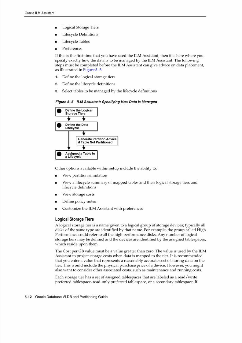
8/16/2019 Oracle Database VLDB and Partitioning Guide
http://slidepdf.com/reader/full/oracle-database-vldb-and-partitioning-guide 166/304

8/16/2019 Oracle Database VLDB and Partitioning Guide
http://slidepdf.com/reader/full/oracle-database-vldb-and-partitioning-guide 167/304

8/16/2019 Oracle Database VLDB and Partitioning Guide
http://slidepdf.com/reader/full/oracle-database-vldb-and-partitioning-guide 168/304
Oracle ILM Assistant
5-14 Oracle Database VLDB and Partitioning Guide
Displays the user-supplied name of the stage.
■ Stage Description
Displays the user-supplied stage description.
■ Action
Displays the action performed when data maps to the stage. Possible actions are:
– Remain Online
– Archive Offline
– Purge
■ Tier Name
Displays the storage tier associated with the stage. For a stage that purges data ormoves data offline, a tier is not specified.
■ Attributes
Displays the optional data attributes that are applied to data when it maps to thestage. Possible values are:
– Compress
– Compress and Read-Only
– Read-Only
■ Stage Duration
Displays the length of time the data can remain mapped to the stage.
■ Stage Start Date
Displays the actual calendar date for the beginning of the stage. The date iscomputed based on the adjacent stages and the user-specified fiscal start date.
■ Stage End Date
Displays the actual calendar date for the end of the stage. The date is computed based on the adjacent stages and the user-specified fiscal start date.
Lifecycle Tables
The Lifecycle Tables area identifies those tables that may be managed by the ILMAssistant, and it is here where these tables are mapped to a lifecycle definition, asillustrated in Figure 5–6. A database may contain many tables, only some of which youwant to consider as candidates for ILM. A table is automatically eligible if it is rangepartitioned on a date column. When the table is associated with a lifecycle definition,the ILM Assistant can manage its data. For tables having no partitioning, storage costsavings and storage tier migration can be modeled using a simulated partitioningstrategy.
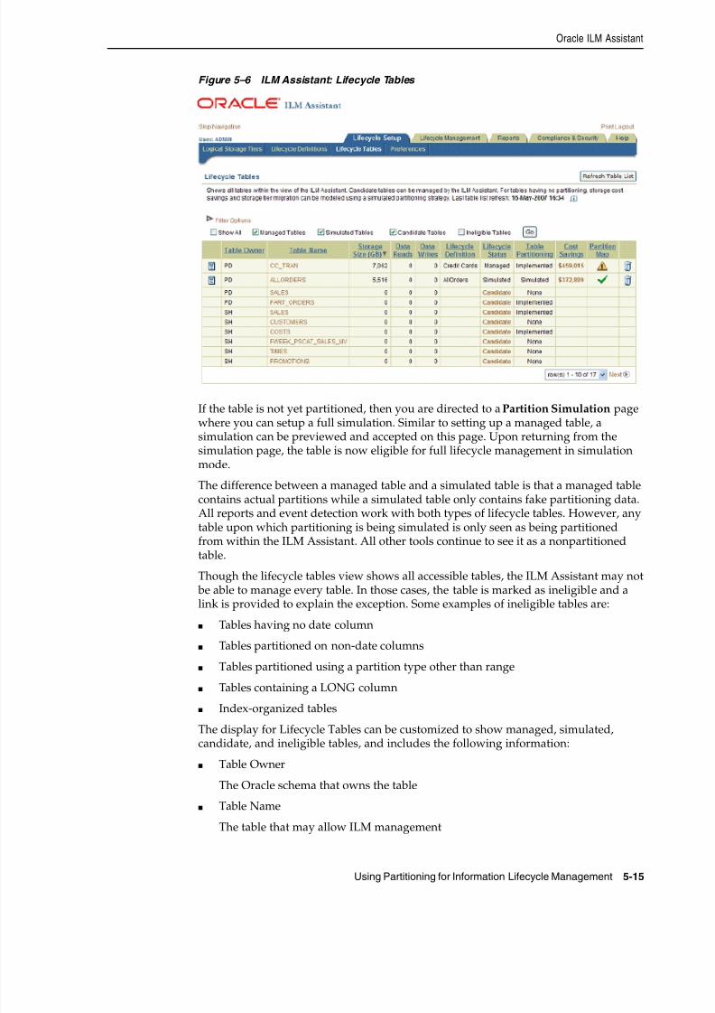
8/16/2019 Oracle Database VLDB and Partitioning Guide
http://slidepdf.com/reader/full/oracle-database-vldb-and-partitioning-guide 169/304
Oracle ILM Assistant
Using Partitioning for Information Lifecycle Management 5-15
Figure 5–6 ILM Assistant: Lifecycle Tables
If the table is not yet partitioned, then you are directed to a Partition Simulation pagewhere you can setup a full simulation. Similar to setting up a managed table, asimulation can be previewed and accepted on this page. Upon returning from thesimulation page, the table is now eligible for full lifecycle management in simulationmode.
The difference between a managed table and a simulated table is that a managed tablecontains actual partitions while a simulated table only contains fake partitioning data.All reports and event detection work with both types of lifecycle tables. However, any
table upon which partitioning is being simulated is only seen as being partitionedfrom within the ILM Assistant. All other tools continue to see it as a nonpartitionedtable.
Though the lifecycle tables view shows all accessible tables, the ILM Assistant may not be able to manage every table. In those cases, the table is marked as ineligible and alink is provided to explain the exception. Some examples of ineligible tables are:
■ Tables having no date column
■ Tables partitioned on non-date columns
■ Tables partitioned using a partition type other than range
■ Tables containing a LONG column
■ Index-organized tablesThe display for Lifecycle Tables can be customized to show managed, simulated,candidate, and ineligible tables, and includes the following information:
■ Table Owner
The Oracle schema that owns the table
■ Table Name
The table that may allow ILM management

8/16/2019 Oracle Database VLDB and Partitioning Guide
http://slidepdf.com/reader/full/oracle-database-vldb-and-partitioning-guide 170/304
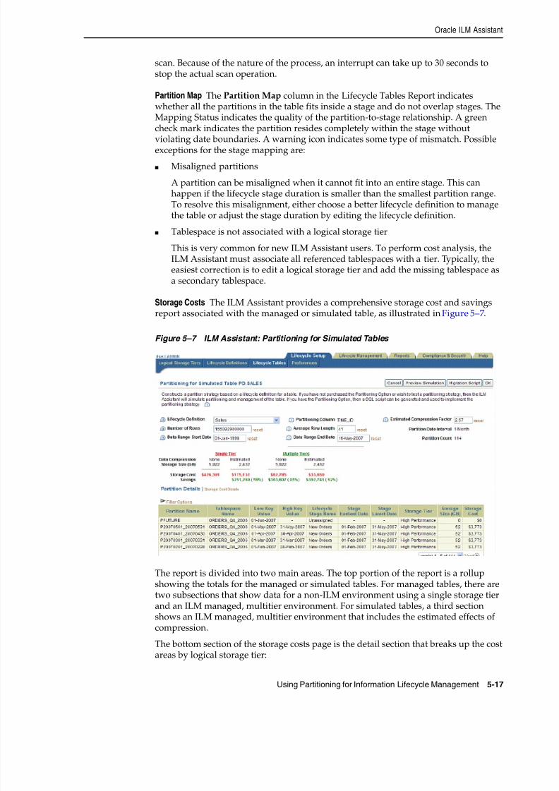
8/16/2019 Oracle Database VLDB and Partitioning Guide
http://slidepdf.com/reader/full/oracle-database-vldb-and-partitioning-guide 171/304
8/16/2019 Oracle Database VLDB and Partitioning Guide
http://slidepdf.com/reader/full/oracle-database-vldb-and-partitioning-guide 172/304
Oracle ILM Assistant
5-18 Oracle Database VLDB and Partitioning Guide
■ Single-Tier Size
Displays the total size of the entities. For a lifecycle-based report, the valuerepresents the sum of all table sizes that are assigned the current lifecycledefinition. For managed tables, the size is the actual size as indicated by thedatabase storage statistics. For simulated tables, the size is the projected size ascalculated by the user-specified number of rows and average row length.
■ Single-Tier Cost
Displays the single-tier cost, which is calculated by multiplying the single-tier sizeof the current entities by the cost of storing the data on the most expensive tierwithin the lifecycle definition.
■ Cost per GB
Displays the user-specified cost when setting up the storage tier. The value is usedto calculate the storage costs for partitions that are assigned to the tier.
■ Multitier Size
Displays the total size of the entities that reside on that tier. For lifecycles, itrepresents all table partitions that are associated with the current tier. For a table, it
represents the sum of all partitions that are associated with the tier. The size doesnot include any projected compression.
■ Multitier Cost
Displays the cost, which is calculated by multiplying the cost per gigabyte for thecurrent tier by the space occupied by the entities. For lifecycles, it represents alltable partitions that are associated with the current tier. For a table, it representsthe sum of all partitions that are associated with the tier.
■ Multitier Savings
Displays the savings, which is computed by subtracting the multitier cost from thecalculated cost of storing the same data using the single-tier approach.
■
Percent SavingsDisplays the ratio of multitier savings to the single-tier cost for the same data.
■ Multitier Compressed Size
Displays the total size of the entities that reside on that tier. For lifecycles, itrepresents all table partitions that are associated with the current tier. For a table, itrepresents the sum of all partitions that are associated with the tier. The sizeincludes projected compression based on the estimated compression factorassigned by the user.
This report item is only present when viewing simulated table data.
■ Multitier Compressed Cost
Displays the cost, which is calculated by multiplying the cost per gigabyte for thecurrent tier by the space occupied by the entities. For lifecycles, it represents alltable partitions that are associated with the current tier. For a table, it representsthe sum of all partitions that are associated with the tier. The size includesprojected compression based on the estimated compression factor assigned by theuser.
This report item is only present when viewing simulated table data.
■ Multitier Compressed Savings
8/16/2019 Oracle Database VLDB and Partitioning Guide
http://slidepdf.com/reader/full/oracle-database-vldb-and-partitioning-guide 173/304
8/16/2019 Oracle Database VLDB and Partitioning Guide
http://slidepdf.com/reader/full/oracle-database-vldb-and-partitioning-guide 174/304
Oracle ILM Assistant
5-20 Oracle Database VLDB and Partitioning Guide
Provide a compression factor. The compression factor is used exclusively by theILM Assistant to estimate storage costs and savings. The factor is purely anestimate, but can give you savings potential. A value of one indicates nocompression is projected. A value greater than one indicates a reduction in spaceusing the formula reduction = 1 / factor. The default value is calculated bysampling a small percentage of the table for compression potential.
An additional option after previewing the simulation is Migration Script generation, asillustrated in Figure 5–7 on page 5-17. This functionality enables the user to create ascript that can convert the existing nonpartitioned table to a partitioned counterpart. Itshould be noted that the script contains a simple create operation and a command tomigrate the existing data; however, parts of the script have been commented out toprevent accidental operation. A conversion of a table to a partitioned table should becarefully planned.
Preferences
Preferences control various aspects of the ILM Assistant's behavior and display of data(for example, the default date format for most entered values and reports, or thedefault number of rows to display). The following preferences can be set:
■ Compression sample block count■ Compression sample percent
■ Date format (Long form)
■ Date format (Short form)
■ Demonstration Mode
Specifies a factor that amplifies the actual table sizes. A value of one effectivelydisables the mode because multiplying a number by one does not change theoriginal value.
■ Language preference
■
Lifecycle table view filterSpecifies the default selection to view when visiting the Lifecycle Tables page.Values can be combined to indicate multiple types of tables. For example, 3indicates that both managed and simulated tables are to be shown. Possible valuesare:
1 - Managed Tables2 - Simulated Tables4 - Candidate Tables8 - Ineligible Tables
The default value is 7, which excludes ineligible tables.
■ Maximum report rows to display
■ Maximum viewable tables
■ Refresh rate for progress monitoring
■ Report column maximum display length
■ Start page for lifecycle setup
Possible values are:
– Logical Storage Tiers

8/16/2019 Oracle Database VLDB and Partitioning Guide
http://slidepdf.com/reader/full/oracle-database-vldb-and-partitioning-guide 175/304
Oracle ILM Assistant
Using Partitioning for Information Lifecycle Management 5-21
– Lifecycle Definitions
– Lifecycle Tables
■ Storage size metric
Specifies the default size metric to be used when viewing storage size values.Possible values are:
KB - KilobytesMB - MegabytesGB - GigabytesTB - Terabytes
The value is case sensitive.
Lifecycle ManagementLifecycle Management is concerned with the tasks that must be performed to movedata to the correct place in the Information Lifecycle. Information is available on thefollowing:
■ Lifecycle Events Calendar■ Lifecycle Events
■ Event Scan History
Lifecycle Events Calendar
The Lifecycle Events Calendar shows the calendar of previous, current, and(optionally,) future lifecycle events that must be performed to place data at theappropriate place in the information lifecycle, as illustrated in Figure 5–5 on page 5-12.You can use the Previous Month with Events button to navigate to previous monthscontaining lifecycle events.
To identify which data must be moved, click the Scan for Events button which asks
whether to scan for all events up to the current day, or into the future. Additionally,you may choose to evaluate all tables or selected tables. The ILM Assistant thencompares the current location of data with where it should be stored in accordancewith the lifecycle definition and recommend the appropriate movement. It also advisesif data should be compressed or set to read only as defined by the lifecycle definition.All the recommendations made by the ILM Assistant are applied to partitions only.
Lifecycle Events
The Lifecycle Events report shows details about data migration events and provides away to generate scripts to perform their actions. You can select some or all of thedisplayed events by clicking the check boxes in the first column. You must selectevents to generate scripts or to dismiss events. To generate a script on the selected
events, click the Generate Script button. To dismiss the selected events to make thempermanently disappear, click the Dismiss Selected Events button.
The event summary shows the following pieces of information:
■ Recommended Action
Indicates the type of event that was detected by the scan operation. Possible eventtypes are:
– MOVE PARTITION
8/16/2019 Oracle Database VLDB and Partitioning Guide
http://slidepdf.com/reader/full/oracle-database-vldb-and-partitioning-guide 176/304
Oracle ILM Assistant
5-22 Oracle Database VLDB and Partitioning Guide
Indicates that a partition should be moved from its current logical storage tierto a new logical storage tier. The movement is achieved by moving thepartition from one tablespace to another.
– COMPRESSION
Indicates that the partition should have data compression enabled.
– READ-ONLYIndicates that the partition should be set to read-only.
– PURGE
Indicates that the partition should be physically deleted.
■ Partition Name
Describes the affected partition.
■ Current Tier
Describes the current location of the partition.
■ Recommended Tier
Describes the target storage tier for move operations.
■ Cost Savings
Indicates the potential storage cost savings if the event action were to beimplemented.
■ Table Owner and Name
Describes the partition table owner and name.
■ Event Date
Indicates the date on which the action should be performed. For events thatshould have been resolved, a single keyword Past is shown; for events in the
future, a calendar date is displayed.■ Event Details
Provides a link to event details. This area describes lifecycle details that affectedthe scan operation.
When a partition requires several logical operations such as move and compress, theILM Assistant displays the operations as separate events. However, in the script, theoperations may be combined into a single SQL DDL statement.
The ILM Assistant currently does not have any archive capability. Therefore, selectingarchive events generates a script that identifies which partitions should now bearchived and lists them as comments.
Event Scan HistoryAny authorized user can invoke event scanning through the Lifecycle EventsCalendar. Over time, tracking the scan activity can be quite difficult, so a history ismade available.
The history report shows the following pieces of information:
■ Scan Date
■ Submitted by User
■ Lowest Event Date
8/16/2019 Oracle Database VLDB and Partitioning Guide
http://slidepdf.com/reader/full/oracle-database-vldb-and-partitioning-guide 177/304
Oracle ILM Assistant
Using Partitioning for Information Lifecycle Management 5-23
■ Highest Event Date
■ Table Owner and Name
■ Number of Events
■ Lifecycle Status
Compliance & SecurityThe Compliance & Security area shows everything that can enforce security and helpmaintain compliance with the numerous regulations from around the world. Itprovides an area to:
■ View Current Status
■ Prove Immutability
■ View Privacy & Security Policies
■ View Auditing
■ Manage Policy Notes
Current Status
Current status summarizes the status of all the various Compliance & Security features that are available. For example, it advises how many Virtual Private Database(VPD) policies have been defined, when a digital signature was last generated, andwhen a comparison of digital signatures was last performed.
Digital Signatures and Immutability
Some regulations stipulate that it must be shown that data has not changed since itwas entered into the database. One technique that can prove that data has not beenaltered is to generate a digital signature.
Oracle Database provides the capability to generate a digital signature for a SQL result
set. This can be generated inside the ILM Assistant and is achieved by creating anamed SQL result set which includes the query to describe the collection of records.The digital signature is generated and is initially saved in a text file.
To show that the data records in a query have not been altered, a digital signature can be presented for a previously defined SQL query, and re-generated on today's data andthe signatures compared, to show that the data has not changed since the digitalsignature was originally generated.
Privacy & Security
The Privacy & Security area enables you to view:
■ A summary of privacy and security definitions for each ILM table
■ Virtual Private Database (VPD) policies
■ Security views on tables managed by the ILM Assistant
■ Reports on the access privileges granted to users for tables managed by the ILMAssistant
By default, the Lifecycle Table Summary is shown and VPD policies and user accessinformation are available by selecting the appropriate links.
8/16/2019 Oracle Database VLDB and Partitioning Guide
http://slidepdf.com/reader/full/oracle-database-vldb-and-partitioning-guide 178/304
Oracle ILM Assistant
5-24 Oracle Database VLDB and Partitioning Guide
Lifecycle Table Summary The Lifecycle Table Summary provides an overview for eachtable regarding which features are being used in terms of VPD policies and tablegrants issued.
Virtual Private Database (VPD) Policies Using standard database privileges, it is possible tolimit access to a table to certain users. However, such access allows users to read allinformation in that table. VPD Policies provide a finer level of control on who can
access information. Using a VPD Policy, it is possible to write sophisticated functions,which define exactly which data is visible to a user.
For example, a policy could say that certain users can only view the last 12 months ofdata, while other users can view all of the data. Another policy could say that the onlydata visible is in the state where the office is located. Therefore, VPD Policies are anextremely powerful tool in controlling access to information. Only VPD policies thathave been defined on tables that are being managed by the ILM Assistant are shownon the VPD Policies report.
Table Access by User The Table Access by User report provides a list of all the accessprivileges granted to users for tables that have been assigned to Lifecycle Definitions.
AuditingSome regulations require that an audit trail be maintained of all access and changes todata. In Oracle Database, several types of auditing are available: database andfine-grained. They each create their own audit records, which can be viewed as oneconsolidated report in the ILM Assistant that can be filtered on several criteria.
Within the auditing area on the ILM Assistant, it is possible to:
■ View the Current Audit Status
■ Manage Fine-Grained Audit Policies
■ View Audit Records
Fine-Grained Auditing Policies Standard Auditing within the Oracle Database logs alltypes of access to a table. However, there may be instances when it is desirable to onlyaudit an event when a certain condition is met (for example, the value of thetransaction being altered is greater than $10,000). This type of auditing is possibleusing Fine-Grained Audit policies where an audit condition can be specified and anoptional function can be called for more sophisticated processing.
View Auditing Records It is possible within the ILM Assistant to view both database andfine-grained audit records for tables mapped to Lifecycle Definitions in the ILMAssistant. An icon represents the type of audit record: database (indicated by a disc) orFGA. Use the Filter condition to filter the audit records that are displayed and click thereport heading to sort the data on that column.
By default, the ILM Assistant only displays audit records for the current day. To seeaudit records for previous days, you must use the filter options to specify a date rangeof records to display.
Policy Notes Policy notes provide textual documentation of your data managementpolicies or anything to document about managing data during its lifetime. Policy notesare informational only; they do not affect the tasks performed by the ILM Assistant.They can be used as a central place to describe your policies, as reminders, and as away to prove that your policies are documented. They can also be used to documentSLA (Service Level Agreements) and to document the compliance rules that you aretrying to enforce.
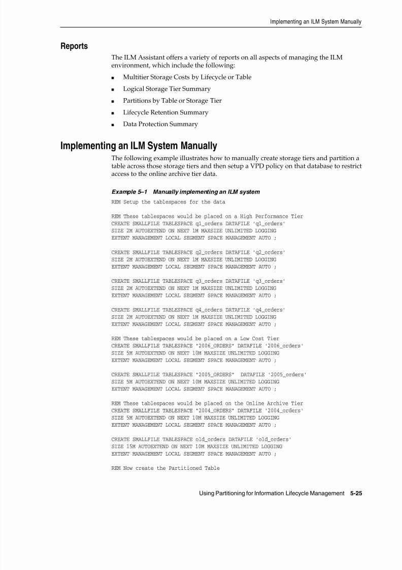
8/16/2019 Oracle Database VLDB and Partitioning Guide
http://slidepdf.com/reader/full/oracle-database-vldb-and-partitioning-guide 179/304
Implementing an ILM System Manually
Using Partitioning for Information Lifecycle Management 5-25
ReportsThe ILM Assistant offers a variety of reports on all aspects of managing the ILMenvironment, which include the following:
■ Multitier Storage Costs by Lifecycle or Table
■ Logical Storage Tier Summary
■ Partitions by Table or Storage Tier
■ Lifecycle Retention Summary
■ Data Protection Summary
Implementing an ILM System ManuallyThe following example illustrates how to manually create storage tiers and partition atable across those storage tiers and then setup a VPD policy on that database to restrictaccess to the online archive tier data.
Example 5–1 Manually implementing an ILM system
REM Setup the tablespaces for the data
REM These tablespaces would be placed on a High Performance TierCREATE SMALLFILE TABLESPACE q1_orders DATAFILE 'q1_orders'SIZE 2M AUTOEXTEND ON NEXT 1M MAXSIZE UNLIMITED LOGGINGEXTENT MANAGEMENT LOCAL SEGMENT SPACE MANAGEMENT AUTO ;
CREATE SMALLFILE TABLESPACE q2_orders DATAFILE 'q2_orders'SIZE 2M AUTOEXTEND ON NEXT 1M MAXSIZE UNLIMITED LOGGINGEXTENT MANAGEMENT LOCAL SEGMENT SPACE MANAGEMENT AUTO ;
CREATE SMALLFILE TABLESPACE q3_orders DATAFILE 'q3_orders'SIZE 2M AUTOEXTEND ON NEXT 1M MAXSIZE UNLIMITED LOGGINGEXTENT MANAGEMENT LOCAL SEGMENT SPACE MANAGEMENT AUTO ;
CREATE SMALLFILE TABLESPACE q4_orders DATAFILE 'q4_orders'SIZE 2M AUTOEXTEND ON NEXT 1M MAXSIZE UNLIMITED LOGGINGEXTENT MANAGEMENT LOCAL SEGMENT SPACE MANAGEMENT AUTO ;
REM These tablespaces would be placed on a Low Cost TierCREATE SMALLFILE TABLESPACE "2006_ORDERS" DATAFILE '2006_orders'SIZE 5M AUTOEXTEND ON NEXT 10M MAXSIZE UNLIMITED LOGGINGEXTENT MANAGEMENT LOCAL SEGMENT SPACE MANAGEMENT AUTO ;
CREATE SMALLFILE TABLESPACE "2005_ORDERS" DATAFILE '2005_orders'SIZE 5M AUTOEXTEND ON NEXT 10M MAXSIZE UNLIMITED LOGGINGEXTENT MANAGEMENT LOCAL SEGMENT SPACE MANAGEMENT AUTO ;
REM These tablespaces would be placed on the Online Archive TierCREATE SMALLFILE TABLESPACE "2004_ORDERS" DATAFILE '2004_orders'SIZE 5M AUTOEXTEND ON NEXT 10M MAXSIZE UNLIMITED LOGGINGEXTENT MANAGEMENT LOCAL SEGMENT SPACE MANAGEMENT AUTO ;
CREATE SMALLFILE TABLESPACE old_orders DATAFILE 'old_orders'SIZE 15M AUTOEXTEND ON NEXT 10M MAXSIZE UNLIMITED LOGGINGEXTENT MANAGEMENT LOCAL SEGMENT SPACE MANAGEMENT AUTO ;
REM Now create the Partitioned Table
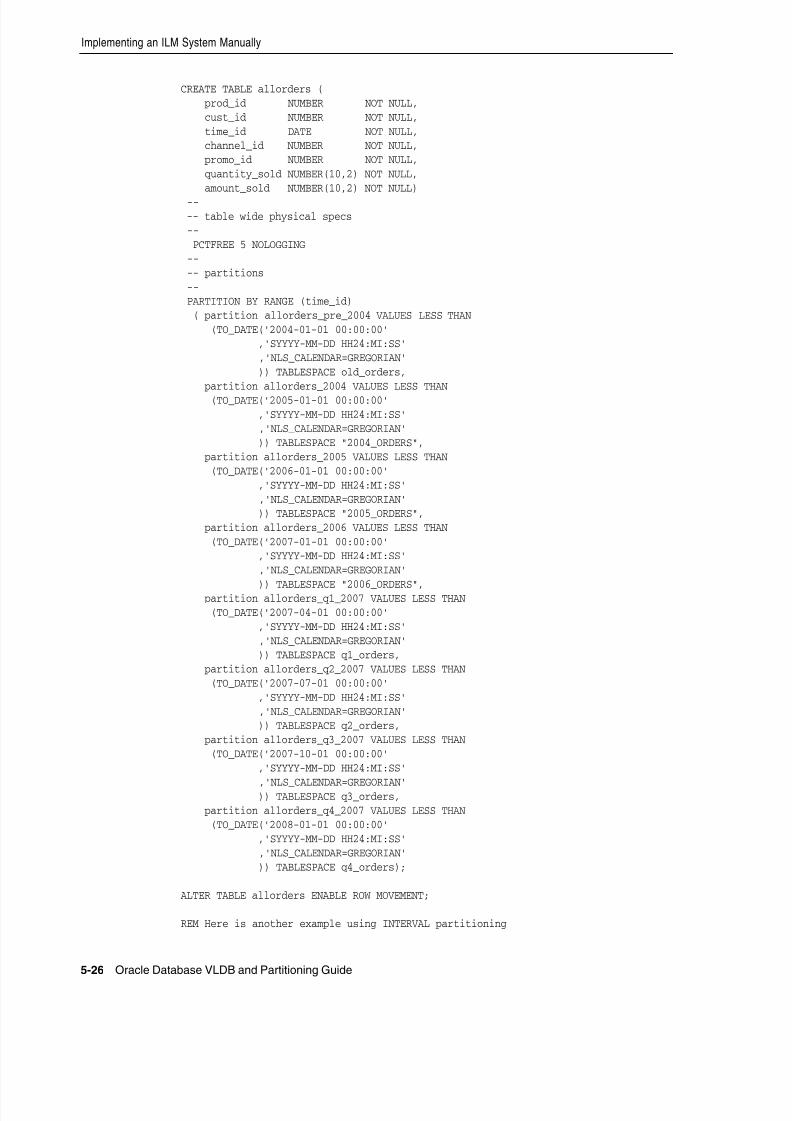
8/16/2019 Oracle Database VLDB and Partitioning Guide
http://slidepdf.com/reader/full/oracle-database-vldb-and-partitioning-guide 180/304
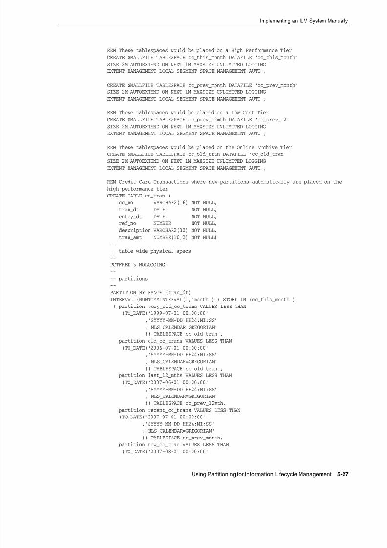
8/16/2019 Oracle Database VLDB and Partitioning Guide
http://slidepdf.com/reader/full/oracle-database-vldb-and-partitioning-guide 181/304
Implementing an ILM System Manually
Using Partitioning for Information Lifecycle Management 5-27
REM These tablespaces would be placed on a High Performance TierCREATE SMALLFILE TABLESPACE cc_this_month DATAFILE 'cc_this_month'SIZE 2M AUTOEXTEND ON NEXT 1M MAXSIZE UNLIMITED LOGGINGEXTENT MANAGEMENT LOCAL SEGMENT SPACE MANAGEMENT AUTO ;
CREATE SMALLFILE TABLESPACE cc_prev_month DATAFILE 'cc_prev_month'SIZE 2M AUTOEXTEND ON NEXT 1M MAXSIZE UNLIMITED LOGGINGEXTENT MANAGEMENT LOCAL SEGMENT SPACE MANAGEMENT AUTO ;
REM These tablespaces would be placed on a Low Cost TierCREATE SMALLFILE TABLESPACE cc_prev_12mth DATAFILE 'cc_prev_12'SIZE 2M AUTOEXTEND ON NEXT 1M MAXSIZE UNLIMITED LOGGINGEXTENT MANAGEMENT LOCAL SEGMENT SPACE MANAGEMENT AUTO ;
REM These tablespaces would be placed on the Online Archive TierCREATE SMALLFILE TABLESPACE cc_old_tran DATAFILE 'cc_old_tran'SIZE 2M AUTOEXTEND ON NEXT 1M MAXSIZE UNLIMITED LOGGINGEXTENT MANAGEMENT LOCAL SEGMENT SPACE MANAGEMENT AUTO ;
REM Credit Card Transactions where new partitions automatically are placed on thehigh performance tierCREATE TABLE cc_tran ( cc_no VARCHAR2(16) NOT NULL, tran_dt DATE NOT NULL, entry_dt DATE NOT NULL, ref_no NUMBER NOT NULL, description VARCHAR2(30) NOT NULL, tran_amt NUMBER(10,2) NOT NULL) -- -- table wide physical specs -- PCTFREE 5 NOLOGGING-- -- partitions
--PARTITION BY RANGE (tran_dt) INTERVAL (NUMTOYMINTERVAL(1,'month') ) STORE IN (cc_this_month ) ( partition very_old_cc_trans VALUES LESS THAN (TO_DATE('1999-07-01 00:00:00' ,'SYYYY-MM-DD HH24:MI:SS' ,'NLS_CALENDAR=GREGORIAN' )) TABLESPACE cc_old_tran , partition old_cc_trans VALUES LESS THAN (TO_DATE('2006-07-01 00:00:00' ,'SYYYY-MM-DD HH24:MI:SS' ,'NLS_CALENDAR=GREGORIAN' )) TABLESPACE cc_old_tran , partition last_12_mths VALUES LESS THAN
(TO_DATE('2007-06-01 00:00:00' ,'SYYYY-MM-DD HH24:MI:SS' ,'NLS_CALENDAR=GREGORIAN' )) TABLESPACE cc_prev_12mth, partition recent_cc_trans VALUES LESS THAN (TO_DATE('2007-07-01 00:00:00' ,'SYYYY-MM-DD HH24:MI:SS' ,'NLS_CALENDAR=GREGORIAN' )) TABLESPACE cc_prev_month, partition new_cc_tran VALUES LESS THAN (TO_DATE('2007-08-01 00:00:00'
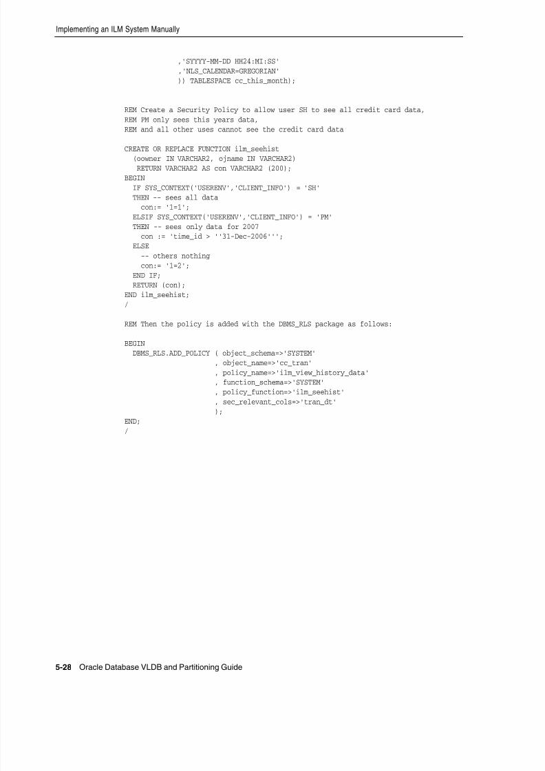
8/16/2019 Oracle Database VLDB and Partitioning Guide
http://slidepdf.com/reader/full/oracle-database-vldb-and-partitioning-guide 182/304
Implementing an ILM System Manually
5-28 Oracle Database VLDB and Partitioning Guide
,'SYYYY-MM-DD HH24:MI:SS' ,'NLS_CALENDAR=GREGORIAN' )) TABLESPACE cc_this_month);
REM Create a Security Policy to allow user SH to see all credit card data,REM PM only sees this years data,REM and all other uses cannot see the credit card data
CREATE OR REPLACE FUNCTION ilm_seehist (oowner IN VARCHAR2, ojname IN VARCHAR2) RETURN VARCHAR2 AS con VARCHAR2 (200);BEGIN IF SYS_CONTEXT('USERENV','CLIENT_INFO') = 'SH' THEN -- sees all data con:= '1=1'; ELSIF SYS_CONTEXT('USERENV','CLIENT_INFO') = 'PM' THEN -- sees only data for 2007 con := 'time_id > ''31-Dec-2006''';ELSE
-- others nothing con:= '1=2'; END IF; RETURN (con);END ilm_seehist;/
REM Then the policy is added with the DBMS_RLS package as follows:
BEGIN DBMS_RLS.ADD_POLICY ( object_schema=>'SYSTEM' , object_name=>'cc_tran' , policy_name=>'ilm_view_history_data' , function_schema=>'SYSTEM' , policy_function=>'ilm_seehist'
, sec_relevant_cols=>'tran_dt' );END;/
8/16/2019 Oracle Database VLDB and Partitioning Guide
http://slidepdf.com/reader/full/oracle-database-vldb-and-partitioning-guide 183/304
8/16/2019 Oracle Database VLDB and Partitioning Guide
http://slidepdf.com/reader/full/oracle-database-vldb-and-partitioning-guide 184/304
Performance
6-2 Oracle Database VLDB and Partitioning Guide
■ More Complex Queries
Bigger DatabasesThe ability to split a large database object into smaller pieces transparently provides benefits to manage a larger total database size. You can identify and manipulateindividual partitions and subpartitions to cope with large database objects. Consider
the following advantages of partitioned objects:
■ Backup and recovery can be performed on a low level of granularity to cope withthe size of the database.
■ Part of a database object can be stored compressed while other parts can remainuncompressed.
■ Partitioning can store data transparently on different storage tiers to lower the costof storing vast amounts of data. Refer to Chapter 5, "Using Partitioning forInformation Lifecycle Management".
Bigger Individual tables: More Rows in Tables
It takes longer to scan a big table than it takes to scan a small table. Queries againstpartitioned tables may access one or more partitions that are small compared with thetotal size of the table. Similarly, queries may take advantage of partition elimination onindexes. It takes less time to read a smaller portion of an index from disk than to readthe entire index. Index structures that share the partitioning strategy with the table,local partitioned indexes, can be accessed and maintained on a partition-by-partition basis.
The database can take advantage of the distinct data sets in separate partitions if youuse parallel execution to speed up queries, DML, and DDL statements. Individualparallel execution servers can work on their own data set, identified by the partition boundaries.
More Users Querying the SystemWith partitioning, users are more likely to hit isolated and smaller data sets.Consequently, the database can return results faster than if all users hit the same andmuch larger data sets. Data contention is less likely.
More Complex QueriesSmaller data sets help perform complex queries faster. If smaller data sets are beingaccessed, then complex calculations are more likely to be processed in memory whichis beneficial from a performance perspective and which reduces the application's I/Orequirements. A larger set may have to be written to the temporary tablespace tocomplete, in which case additional I/O against the database storage occurs.
PerformanceGood performance is a key to success for a data warehouse. Analyses run against thedatabase should return within a reasonable amount of time, even if the queries accesslarge amounts of data in tables that are terabytes in size. Partitioning providesfundamental functionality to enable successful data warehouses that are notprohibitively expensive in terms of hardware cost.
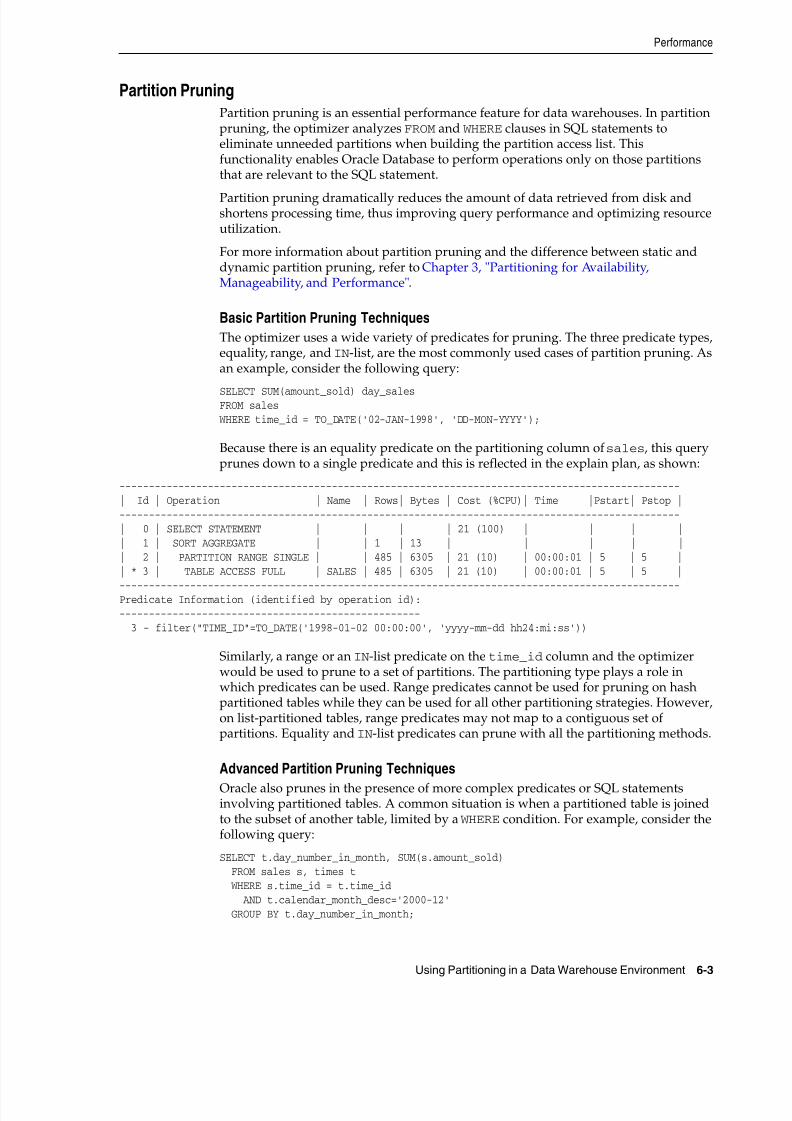
8/16/2019 Oracle Database VLDB and Partitioning Guide
http://slidepdf.com/reader/full/oracle-database-vldb-and-partitioning-guide 185/304
Performance
Using Partitioning in a Data Warehouse Environment 6-3
Partition PruningPartition pruning is an essential performance feature for data warehouses. In partitionpruning, the optimizer analyzes FROM and WHERE clauses in SQL statements toeliminate unneeded partitions when building the partition access list. Thisfunctionality enables Oracle Database to perform operations only on those partitionsthat are relevant to the SQL statement.
Partition pruning dramatically reduces the amount of data retrieved from disk andshortens processing time, thus improving query performance and optimizing resourceutilization.
For more information about partition pruning and the difference between static anddynamic partition pruning, refer to Chapter 3, "Partitioning for Availability,Manageability, and Performance".
Basic Partition Pruning Techniques
The optimizer uses a wide variety of predicates for pruning. The three predicate types,equality, range, and IN-list, are the most commonly used cases of partition pruning. Asan example, consider the following query:
SELECT SUM(amount_sold) day_salesFROM sales
WHERE time_id = TO_DATE('02-JAN-1998', 'DD-MON-YYYY');
Because there is an equality predicate on the partitioning column of sales, this queryprunes down to a single predicate and this is reflected in the explain plan, as shown:
-----------------------------------------------------------------------------------------------| Id | Operation | Name | Rows| Bytes | Cost (%CPU)| Time |Pstart| Pstop |-----------------------------------------------------------------------------------------------| 0 | SELECT STATEMENT | | | | 21 (100) | | | || 1 | SORT AGGREGATE | | 1 | 13 | | | | || 2 | PARTITION RANGE SINGLE | | 485 | 6305 | 21 (10) | 00:00:01 | 5 | 5 || * 3 | TABLE ACCESS FULL | SALES | 485 | 6305 | 21 (10) | 00:00:01 | 5 | 5 |
-----------------------------------------------------------------------------------------------Predicate Information (identified by operation id):---------------------------------------------------3 - filter("TIME_ID"=TO_DATE('1998-01-02 00:00:00', 'yyyy-mm-dd hh24:mi:ss'))
Similarly, a range or an IN-list predicate on the time_id column and the optimizerwould be used to prune to a set of partitions. The partitioning type plays a role inwhich predicates can be used. Range predicates cannot be used for pruning on hashpartitioned tables while they can be used for all other partitioning strategies. However,on list-partitioned tables, range predicates may not map to a contiguous set ofpartitions. Equality and IN-list predicates can prune with all the partitioning methods.
Advanced Partition Pruning Techniques
Oracle also prunes in the presence of more complex predicates or SQL statementsinvolving partitioned tables. A common situation is when a partitioned table is joinedto the subset of another table, limited by a WHERE condition. For example, consider thefollowing query:
SELECT t.day_number_in_month, SUM(s.amount_sold) FROM sales s, times t WHERE s.time_id = t.time_id AND t.calendar_month_desc='2000-12' GROUP BY t.day_number_in_month;
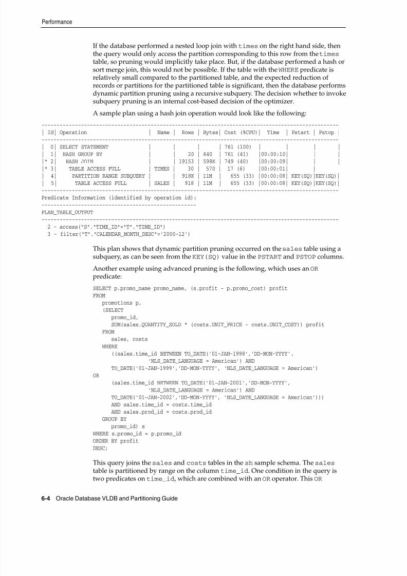
8/16/2019 Oracle Database VLDB and Partitioning Guide
http://slidepdf.com/reader/full/oracle-database-vldb-and-partitioning-guide 186/304
Performance
6-4 Oracle Database VLDB and Partitioning Guide
If the database performed a nested loop join with times on the right hand side, thenthe query would only access the partition corresponding to this row from the times table, so pruning would implicitly take place. But, if the database performed a hash orsort merge join, this would not be possible. If the table with the WHERE predicate isrelatively small compared to the partitioned table, and the expected reduction ofrecords or partitions for the partitioned table is significant, then the database performsdynamic partition pruning using a recursive subquery. The decision whether to invoke
subquery pruning is an internal cost-based decision of the optimizer.
A sample plan using a hash join operation would look like the following:
--------------------------------------------------------------------------------------------------| Id| Operation | Name | Rows | Bytes| Cost (%CPU)| Time | Pstart | Pstop |--------------------------------------------------------------------------------------------------| 0| SELECT STATEMENT | | | | 761 (100) | | | || 1| HASH GROUP BY | | 20 | 640 | 761 (41) |00:00:10| | ||* 2| HASH JOIN | | 19153 | 598K | 749 (40) |00:00:09| | ||* 3| TABLE ACCESS FULL | TIMES | 30 | 570 | 17 (6) |00:00:01| | || 4| PARTITION RANGE SUBQUERY | | 918K | 11M | 655 (33) |00:00:08| KEY(SQ)|KEY(SQ)|| 5| TABLE ACCESS FULL | SALES | 918 | 11M | 655 (33) |00:00:08| KEY(SQ)|KEY(SQ)|--------------------------------------------------------------------------------------------------Predicate Information (identified by operation id):---------------------------------------------------PLAN_TABLE_OUTPUT-------------------------------------------------------------------------------------------------- 2 - access("S"."TIME_ID"="T"."TIME_ID")3 - filter("T"."CALENDAR_MONTH_DESC"='2000-12')
This plan shows that dynamic partition pruning occurred on the sales table using asubquery, as can be seen from the KEY(SQ) value in the PSTART and PSTOP columns.
Another example using advanced pruning is the following, which uses an OR predicate:
SELECT p.promo_name promo_name, (s.profit - p.promo_cost) profitFROM
promotions p, (SELECT promo_id, SUM(sales.QUANTITY_SOLD * (costs.UNIT_PRICE - costs.UNIT_COST)) profit FROM sales, costs WHERE ((sales.time_id BETWEEN TO_DATE('01-JAN-1998','DD-MON-YYYY', 'NLS_DATE_LANGUAGE = American') AND TO_DATE('01-JAN-1999','DD-MON-YYYY', 'NLS_DATE_LANGUAGE = American')OR (sales.time_id BETWEEN TO_DATE('01-JAN-2001','DD-MON-YYYY', 'NLS_DATE_LANGUAGE = American') AND TO_DATE('01-JAN-2002','DD-MON-YYYY', 'NLS_DATE_LANGUAGE = American')))
AND sales.time_id = costs.time_id AND sales.prod_id = costs.prod_id GROUP BY promo_id) s
WHERE s.promo_id = p.promo_idORDER BY profitDESC;
This query joins the sales and costs tables in the sh sample schema. The sales table is partitioned by range on the column time_id. One condition in the query istwo predicates on time_id, which are combined with an OR operator. This OR
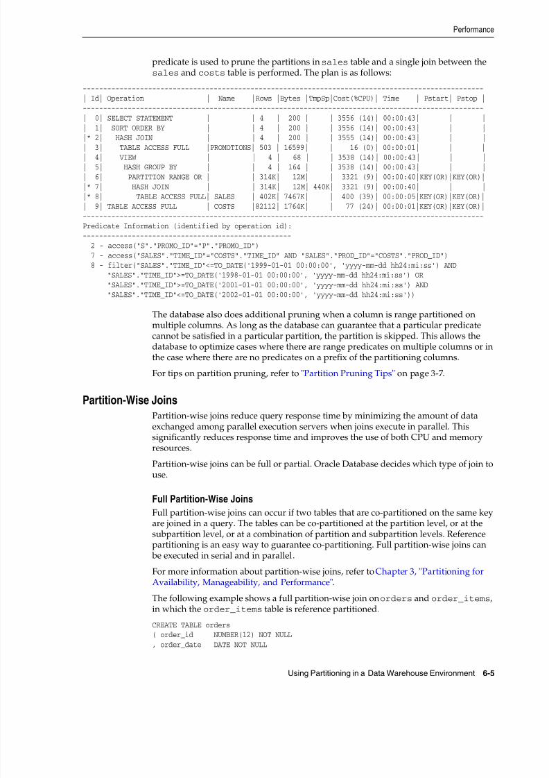
8/16/2019 Oracle Database VLDB and Partitioning Guide
http://slidepdf.com/reader/full/oracle-database-vldb-and-partitioning-guide 187/304
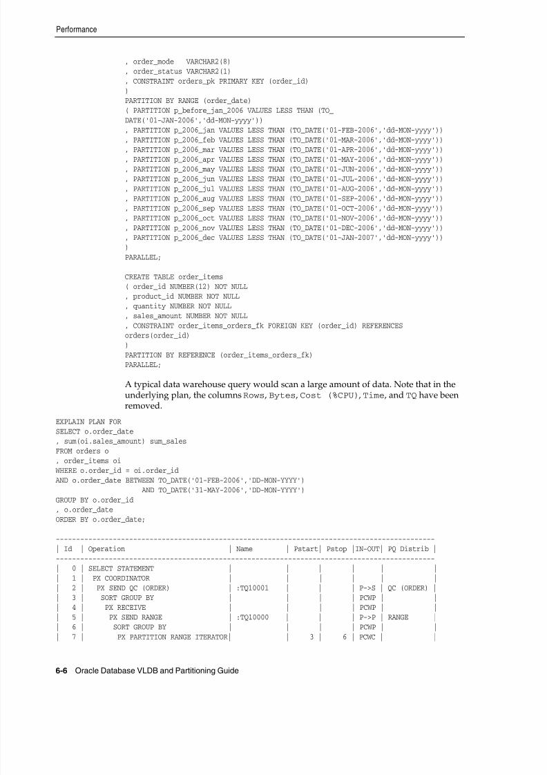
8/16/2019 Oracle Database VLDB and Partitioning Guide
http://slidepdf.com/reader/full/oracle-database-vldb-and-partitioning-guide 188/304
Performance
6-6 Oracle Database VLDB and Partitioning Guide
, order_mode VARCHAR2(8), order_status VARCHAR2(1), CONSTRAINT orders_pk PRIMARY KEY (order_id))PARTITION BY RANGE (order_date)( PARTITION p_before_jan_2006 VALUES LESS THAN (TO_DATE('01-JAN-2006','dd-MON-yyyy')), PARTITION p_2006_jan VALUES LESS THAN (TO_DATE('01-FEB-2006','dd-MON-yyyy')), PARTITION p_2006_feb VALUES LESS THAN (TO_DATE('01-MAR-2006','dd-MON-yyyy')), PARTITION p_2006_mar VALUES LESS THAN (TO_DATE('01-APR-2006','dd-MON-yyyy')), PARTITION p_2006_apr VALUES LESS THAN (TO_DATE('01-MAY-2006','dd-MON-yyyy')), PARTITION p_2006_may VALUES LESS THAN (TO_DATE('01-JUN-2006','dd-MON-yyyy')), PARTITION p_2006_jun VALUES LESS THAN (TO_DATE('01-JUL-2006','dd-MON-yyyy')), PARTITION p_2006_jul VALUES LESS THAN (TO_DATE('01-AUG-2006','dd-MON-yyyy')), PARTITION p_2006_aug VALUES LESS THAN (TO_DATE('01-SEP-2006','dd-MON-yyyy')), PARTITION p_2006_sep VALUES LESS THAN (TO_DATE('01-OCT-2006','dd-MON-yyyy')), PARTITION p_2006_oct VALUES LESS THAN (TO_DATE('01-NOV-2006','dd-MON-yyyy')), PARTITION p_2006_nov VALUES LESS THAN (TO_DATE('01-DEC-2006','dd-MON-yyyy')), PARTITION p_2006_dec VALUES LESS THAN (TO_DATE('01-JAN-2007','dd-MON-yyyy')))PARALLEL;
CREATE TABLE order_items( order_id NUMBER(12) NOT NULL, product_id NUMBER NOT NULL, quantity NUMBER NOT NULL, sales_amount NUMBER NOT NULL, CONSTRAINT order_items_orders_fk FOREIGN KEY (order_id) REFERENCESorders(order_id))PARTITION BY REFERENCE (order_items_orders_fk)PARALLEL;
A typical data warehouse query would scan a large amount of data. Note that in theunderlying plan, the columns Rows, Bytes, Cost (%CPU), Time, and TQ have been
removed.EXPLAIN PLAN FORSELECT o.order_date, sum(oi.sales_amount) sum_salesFROM orders o, order_items oi
WHERE o.order_id = oi.order_idAND o.order_date BETWEEN TO_DATE('01-FEB-2006','DD-MON-YYYY') AND TO_DATE('31-MAY-2006','DD-MON-YYYY')GROUP BY o.order_id, o.order_dateORDER BY o.order_date;
---------------------------------------------------------------------------------------------| Id | Operation | Name | Pstart| Pstop |IN-OUT| PQ Distrib |---------------------------------------------------------------------------------------------| 0 | SELECT STATEMENT | | | | | || 1 | PX COORDINATOR | | | | | || 2 | PX SEND QC (ORDER) | :TQ10001 | | | P->S | QC (ORDER) || 3 | SORT GROUP BY | | | | PCWP | || 4 | PX RECEIVE | | | | PCWP | || 5 | PX SEND RANGE | :TQ10000 | | | P->P | RANGE || 6 | SORT GROUP BY | | | | PCWP | || 7 | PX PARTITION RANGE ITERATOR| | 3 | 6 | PCWC | |
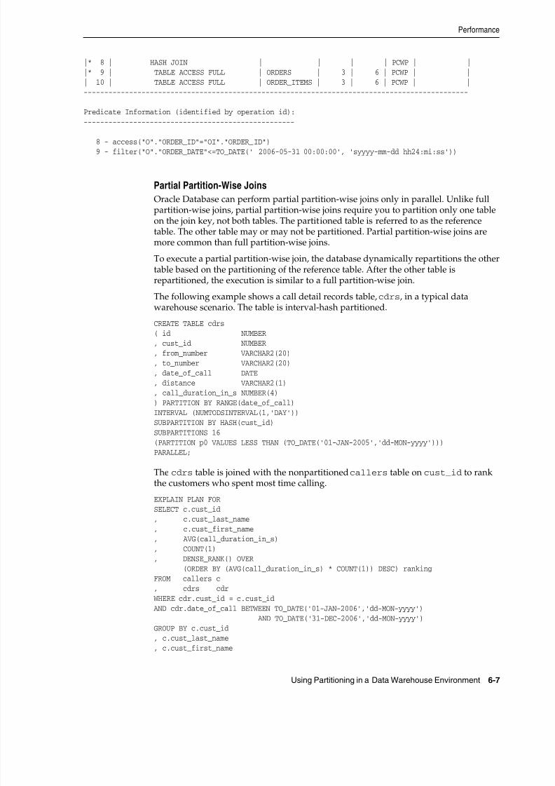
8/16/2019 Oracle Database VLDB and Partitioning Guide
http://slidepdf.com/reader/full/oracle-database-vldb-and-partitioning-guide 189/304
Performance
Using Partitioning in a Data Warehouse Environment 6-7
|* 8 | HASH JOIN | | | | PCWP | ||* 9 | TABLE ACCESS FULL | ORDERS | 3 | 6 | PCWP | || 10 | TABLE ACCESS FULL | ORDER_ITEMS | 3 | 6 | PCWP | |---------------------------------------------------------------------------------------------
Predicate Information (identified by operation id):---------------------------------------------------
8 - access("O"."ORDER_ID"="OI"."ORDER_ID") 9 - filter("O"."ORDER_DATE"<=TO_DATE(' 2006-05-31 00:00:00', 'syyyy-mm-dd hh24:mi:ss'))
Partial Partition-Wise Joins
Oracle Database can perform partial partition-wise joins only in parallel. Unlike fullpartition-wise joins, partial partition-wise joins require you to partition only one tableon the join key, not both tables. The partitioned table is referred to as the referencetable. The other table may or may not be partitioned. Partial partition-wise joins aremore common than full partition-wise joins.
To execute a partial partition-wise join, the database dynamically repartitions the othertable based on the partitioning of the reference table. After the other table isrepartitioned, the execution is similar to a full partition-wise join.
The following example shows a call detail records table, cdrs, in a typical datawarehouse scenario. The table is interval-hash partitioned.
CREATE TABLE cdrs( id NUMBER, cust_id NUMBER, from_number VARCHAR2(20), to_number VARCHAR2(20), date_of_call DATE, distance VARCHAR2(1), call_duration_in_s NUMBER(4)) PARTITION BY RANGE(date_of_call)
INTERVAL (NUMTODSINTERVAL(1,'DAY'))SUBPARTITION BY HASH(cust_id)SUBPARTITIONS 16(PARTITION p0 VALUES LESS THAN (TO_DATE('01-JAN-2005','dd-MON-yyyy')))PARALLEL;
The cdrs table is joined with the nonpartitioned callers table on cust_id to rankthe customers who spent most time calling.
EXPLAIN PLAN FORSELECT c.cust_id, c.cust_last_name, c.cust_first_name, AVG(call_duration_in_s)
, COUNT(1), DENSE_RANK() OVER (ORDER BY (AVG(call_duration_in_s) * COUNT(1)) DESC) rankingFROM callers c, cdrs cdr
WHERE cdr.cust_id = c.cust_idAND cdr.date_of_call BETWEEN TO_DATE('01-JAN-2006','dd-MON-yyyy') AND TO_DATE('31-DEC-2006','dd-MON-yyyy')GROUP BY c.cust_id, c.cust_last_name, c.cust_first_name
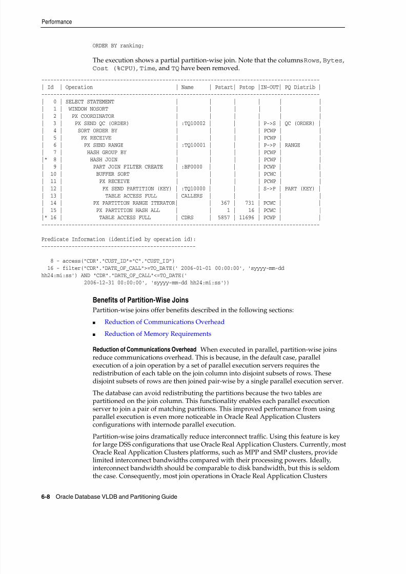
8/16/2019 Oracle Database VLDB and Partitioning Guide
http://slidepdf.com/reader/full/oracle-database-vldb-and-partitioning-guide 190/304
Performance
6-8 Oracle Database VLDB and Partitioning Guide
ORDER BY ranking;
The execution shows a partial partition-wise join. Note that the columns Rows, Bytes,Cost (%CPU), Time, and TQ have been removed.
--------------------------------------------------------------------------------------------| Id | Operation | Name | Pstart| Pstop |IN-OUT| PQ Distrib |--------------------------------------------------------------------------------------------
| 0 | SELECT STATEMENT | | | | | || 1 | WINDOW NOSORT | | | | | || 2 | PX COORDINATOR | | | | | || 3 | PX SEND QC (ORDER) | :TQ10002 | | | P->S | QC (ORDER) || 4 | SORT ORDER BY | | | | PCWP | || 5 | PX RECEIVE | | | | PCWP | || 6 | PX SEND RANGE | :TQ10001 | | | P->P | RANGE || 7 | HASH GROUP BY | | | | PCWP | ||* 8 | HASH JOIN | | | | PCWP | || 9 | PART JOIN FILTER CREATE | :BF0000 | | | PCWP | || 10 | BUFFER SORT | | | | PCWC | || 11 | PX RECEIVE | | | | PCWP | || 12 | PX SEND PARTITION (KEY) | :TQ10000 | | | S->P | PART (KEY) || 13 | TABLE ACCESS FULL | CALLERS | | | | |
| 14 | PX PARTITION RANGE ITERATOR| | 367 | 731 | PCWC | || 15 | PX PARTITION HASH ALL | | 1 | 16 | PCWC | ||* 16 | TABLE ACCESS FULL | CDRS | 5857 | 11696 | PCWP | |--------------------------------------------------------------------------------------------
Predicate Information (identified by operation id):---------------------------------------------------
8 - access("CDR"."CUST_ID"="C"."CUST_ID") 16 - filter("CDR"."DATE_OF_CALL">=TO_DATE(' 2006-01-01 00:00:00', 'syyyy-mm-ddhh24:mi:ss') AND "CDR"."DATE_OF_CALL"<=TO_DATE(' 2006-12-31 00:00:00', 'syyyy-mm-dd hh24:mi:ss'))
Benefits of Partition-Wise JoinsPartition-wise joins offer benefits described in the following sections:
■ Reduction of Communications Overhead
■ Reduction of Memory Requirements
Reduction of Communications Overhead When executed in parallel, partition-wise joinsreduce communications overhead. This is because, in the default case, parallelexecution of a join operation by a set of parallel execution servers requires theredistribution of each table on the join column into disjoint subsets of rows. Thesedisjoint subsets of rows are then joined pair-wise by a single parallel execution server.
The database can avoid redistributing the partitions because the two tables are
partitioned on the join column. This functionality enables each parallel executionserver to join a pair of matching partitions. This improved performance from usingparallel execution is even more noticeable in Oracle Real Application Clustersconfigurations with internode parallel execution.
Partition-wise joins dramatically reduce interconnect traffic. Using this feature is keyfor large DSS configurations that use Oracle Real Application Clusters. Currently, mostOracle Real Application Clusters platforms, such as MPP and SMP clusters, providelimited interconnect bandwidths compared with their processing powers. Ideally,interconnect bandwidth should be comparable to disk bandwidth, but this is seldomthe case. Consequently, most join operations in Oracle Real Application Clusters
8/16/2019 Oracle Database VLDB and Partitioning Guide
http://slidepdf.com/reader/full/oracle-database-vldb-and-partitioning-guide 191/304
Performance
Using Partitioning in a Data Warehouse Environment 6-9
experience high interconnect latencies without parallel execution of partition-wise joins.
Reduction of Memory Requirements Partition-wise joins require less memory than theequivalent join operation of the complete data set of the tables being joined. For serial joins, the join is performed at the same time on a pair of matching partitions. If data isevenly distributed across partitions, then the memory requirement is divided by the
number of partitions. There is no skew.
In the parallel case, memory requirements depend on the number of partition pairsthat are joined in parallel. For example, if the degree of parallelism is 20 and thenumber of partitions is 100, then 5 times less memory is required because only 20 joinsof two partitions are performed at the same time. The fact that partition-wise joinsrequire less memory has a direct effect on performance. For example, the join probablydoes not need to write blocks to disk during the build phase of a hash join.
Performance Considerations for Parallel Partition-Wise Joins
The optimizer weighs the advantages and disadvantages when deciding whether touse partition-wise joins.
■ In range partitioning where partition sizes differ, data skew increases responsetime; some parallel execution servers take longer than others to finish their joins.Oracle recommends the use of hash partitioning and subpartitioning to enablepartition-wise joins because hash partitioning, if the number of partitions is apower of two, limits the risk of skew. Ideally, the hash partitioning key is uniqueor almost unique to minimize the risk of skew.
■ The number of partitions used for partition-wise joins should, if possible, be amultiple of the number of query servers. With a degree of parallelism of 16, forexample, you can have 16, 32, or even 64 partitions. If there is an odd number ofpartitions, then some parallel execution servers are used less than others. Forexample, if there are 17 evenly distributed partition pairs, only one pair works onthe last join, while the other pairs has to wait. This is because, in the beginning of
the execution, each parallel execution server works on a different partition pair.After this first phase, only one pair is left. Thus, a single parallel execution server joins this remaining pair while all other parallel execution servers are idle.
Sometimes, parallel joins can cause remote I/Os. For example, on Oracle RealApplication Clusters environments running on MPP configurations, if a pair ofmatching partitions is not collocated on the same node, a partition-wise join requiresextra internode communication due to remote I/O. This is because Oracle musttransfer at least one partition to the node where the join is performed. In this case, it is better to explicitly redistribute the data than to use a partition-wise join.
Indexes and Partitioned IndexesIndexes are optional structures associated with tables that allow SQL statements toexecute more quickly against a table. Even though table scans are very common inmany data warehouses, indexes can often speed up queries. The most commonly usedindexes in a data warehouse are B-tree and bitmap indexes.
Both B-tree and bitmap indexes can be created as local indexes on a partitioned table,in which case they inherit the table's partitioning strategy. B-tree indexes can becreated as global partitioned indexes on partitioned and on nonpartitioned tables.
For more information about partitioned indexes, refer to Chapter 3, "Partitioning forAvailability, Manageability, and Performance".
8/16/2019 Oracle Database VLDB and Partitioning Guide
http://slidepdf.com/reader/full/oracle-database-vldb-and-partitioning-guide 192/304
Performance
6-10 Oracle Database VLDB and Partitioning Guide
Local Partitioned Indexes
In a local index, all keys in a particular index partition refer only to rows stored in asingle underlying table partition. A local index is equipartitioned with the underlyingtable. Oracle partitions the index on the same columns as the underlying table, createsthe same number of partitions or subpartitions, and gives them the same partition bounds as corresponding partitions of the underlying table.
Oracle also maintains the index partitioning automatically when partitions in theunderlying table are added, dropped, merged, or split, or when hash partitions orsubpartitions are added or coalesced. This ensures that the index remainsequipartitioned with the table.
For data warehouse applications, local nonprefixed indexes can improve performance because many index partitions can be scanned in parallel by range queries on theindex key. The following example creates a local B-tree index on a partitionedcustomers table.
ALTER SESSION enable parallel ddl;
CREATE INDEX cust_last_name_ixON customers(last_name) LOCAL
PARALLEL NOLOGGING ;
Bitmap indexes use a very efficient storage mechanism for low cardinality columns.Bitmap indexes are commonly used in data warehouses, especially in data warehousesthat implement so-called star schemas. A single star schema consists of a central largefact table and multiple smaller dimension tables that describe the data in the fact table.
For example, the sales table in the sample sh schema in the Oracle database is a facttable, that is described by dimension tables customers, products, promotions,times, and channels. Bitmap indexes enable the so-called star transformation, anoptimization for fast query retrieval against star or star look-a-like schemas.
Fact table foreign key columns are ideal candidates for bitmap indexes, becausegenerally there are relatively few distinct values relative to the total number of rows.
Fact tables are often range or range-* partitioned, in which case you must create local bitmap indexes. Global bitmap indexes on partitioned tables are not supported.
The following example creates a local partitioned bitmap index on the sales table.
ALTER SESSION enable parallel ddl;
CREATE BITMAP INDEX prod_id_ixON sales(prod_id) LOCALPARALLEL NOLOGGING;
Nonpartitioned Indexes
You can create nonpartitioned indexes on nonpartitioned tables and on partitionedtables. Nonpartitioned indexes are primarily used on nonpartitioned tables in datawarehouse environments. You can use a nonpartitioned global index on a partitionedtable to enforce a primary or unique key. A nonpartitioned (global) index can be usefulfor queries that commonly retrieve very few rows based on equality predicates orin-list on a column or set of columns that is not included in the partitioning key. Inthose cases, it can be faster to scan a single index than to scan many index partitions tofind all matching rows.
See Also: Oracle Database Data Warehousing Guide for moreinformation about the star transformation
8/16/2019 Oracle Database VLDB and Partitioning Guide
http://slidepdf.com/reader/full/oracle-database-vldb-and-partitioning-guide 193/304
8/16/2019 Oracle Database VLDB and Partitioning Guide
http://slidepdf.com/reader/full/oracle-database-vldb-and-partitioning-guide 194/304
Performance
6-12 Oracle Database VLDB and Partitioning Guide
Partitioning and Data Compression
Data in a partitioned table can be compressed on a partition-by-partition basis. Usingcompressed data is most efficient for data that does not change frequently. AlthoughOracle Database 11 g supports compression for all DML operations, it is still moreefficient to modify data in a non-compressed table.
Common data warehouse scenarios often see few data changes as data ages and other
scenarios only insert data. Using the partition management features, you can compressdata on a partition-by-partition basis. Note that altering a partition to enablecompression only applies to future data to be inserted into the partition. To compressthe existing data in the partition, you must move the partition. Enabling compressionand moving a partition can be done in a single operation.
To use table compression on partitioned tables with bitmap indexes, you must do thefollowing before you introduce the compression attribute for the first time:
1. Mark bitmap indexes unusable.
2. Set the compression attribute.
3. Rebuild the indexes.
The first time you make a compressed partition part of an existing, fullyuncompressed partitioned table, you must either drop all existing bitmap indexes ormark them UNUSABLE before adding a compressed partition. This must be doneregardless of whether any partition contains data. It is also independent of theoperation that causes one or more compressed partitions to become part of the table.This does not apply to a partitioned table having B-tree indexes only.
The following example shows how to compress the SALES_1995 partition in thesales table.
ALTER SESSION enable parallel ddl;
ALTER TABLE salesMOVE PARTITION sales_1995COMPRESS FOR OLTPPARALLEL NOLOGGING;
If a table or a partition takes less space on disk, then the performance of large tablescans in an I/O-constraint environment may improve.
Materialized Views and Partitioning
One technique employed in data warehouses to improve performance is the creationof summaries. Summaries are special types of aggregate views that improve queryexecution times by precalculating expensive joins and aggregation operations beforeexecution and storing the results in a table in the database. For example, you can createa summary table to contain the sums of sales by region and by product.
The summaries or aggregates that are referred to in this book and in literature on datawarehousing are created in Oracle Database using a schema object called amaterialized view. Materialized views in a data warehouse are meant to speed upquery performance.
The database supports transparent rewrites against materialized views, so that you donot need to modify the original queries to take advantage of precalculated results inmaterialized views. Instead of executing the query, the database retrievesprecalculated results from one or more materialized views, perform any necessaryadditional operations on the data, and return the query results. The database
8/16/2019 Oracle Database VLDB and Partitioning Guide
http://slidepdf.com/reader/full/oracle-database-vldb-and-partitioning-guide 195/304
Manageability
Using Partitioning in a Data Warehouse Environment 6-13
guarantees correct results in line with your setting of the QUERY_REWRITE_INTEGRITY initialization parameter.
Partitioned Materialized Views The underlying storage for a materialized view is a tablestructure. You can partition materialized views like you can partition tables. When the
database rewrites a query to run against materialized views, the query can takeadvantage of the same performance features that queries running against tablesdirectly benefit from. The rewritten query may eliminate materialized view partitions.If joins back to tables or with other materialized views are necessary to retrieve thequery result, then the rewritten query can take advantage of partition-wise joins.
The following example shows how to create a compressed partitioned materializedview that aggregates sales results to country level. This materialized view benefitsfrom queries that summarize sales numbers by country level or higher to subregion orregion level.
ALTER SESSION ENABLE PARALLEL DDL;
CREATE MATERIALIZED VIEW country_sales
PARTITION BY HASH (country_id)PARTITIONS 16COMPRESS FOR OLTPPARALLEL NOLOGGINGENABLE QUERY REWRITEAS SELECT co.country_id, co.country_name, co.country_subregion, co.country_region, sum(sa.quantity_sold) country_quantity_sold, sum(sa.amount_sold) country_amount_soldFROM sales sa, customers cu, countries co
WHERE sa.cust_id = cu.cust_idAND cu.country_id = co.country_idGROUP BY co.country_id, co.country_name, co.country_subregion, co.country_region;
ManageabilityData Warehouses store historical data. An important part of a data warehouse is the
data load and purge. Partitioning is powerful technology that can help datamanagement for data warehousing.
Partition Exchange LoadPartitions can be added using Partition Exchange Load (PEL). When you use PEL, youcreate a separate table that looks exactly like a single partition, including the sameindexes and constraints, if any. If you use a composite partitioned table, then yourseparate table must use a partitioning strategy that matches the subpartitioningstrategy of your composite partitioned table. You can then swap out an existing table
See Also: Oracle Database Data Warehousing Guide
See Also: Oracle Database Data Warehousing Guide
8/16/2019 Oracle Database VLDB and Partitioning Guide
http://slidepdf.com/reader/full/oracle-database-vldb-and-partitioning-guide 196/304

8/16/2019 Oracle Database VLDB and Partitioning Guide
http://slidepdf.com/reader/full/oracle-database-vldb-and-partitioning-guide 197/304
Manageability
Using Partitioning in a Data Warehouse Environment 6-15
Partitioning and Materialized View Refresh StrategiesThere are different ways to keep materialized views updated:
■ Full refresh
■ Fast (incremental) refresh based on materialized view logs against the base tables
■ Manually using DML, followed by ALTER MATERIALIZED VIEW CONSIDER
FRESH
To enable query rewrites, set the QUERY_REWRITE_INTEGRITY initializationparameter. If you manually keep materialized views up to date, then you must setQUERY_REWRITE_INTEGRITY to either TRUSTED or STALE_TOLERATED.
If your materialized views and base tables use comparable partitioning strategies, thenPEL can be an extremely powerful way to keep materialized views up-to-datemanually. For example, if both your base table and your materialized view use rangepartitioning, then you can consider PEL to keep your base table and materialized viewup-to-date. The total data refresh scenario would work as follows:
■ Create tables to enable PEL against the tables and materialized views
■ Load data into the tables, build the indexes, and implement any constraints
■ Update the base tables using PEL
■ Update the materialized views using PEL
■ Execute ALTER MATERIALIZED VIEW CONSIDER FRESH for every materializedview you updated using this strategy
Note that this strategy implies a short interval, in between PEL against the base tableand PEL against the materialized view, in which the materialized view does not reflectthe current data in the underlying tables. Consider the QUERY_REWRITE_INTEGRITY setting and the activity on your system to identify whether you can cope with this
situation.
Removing Data from TablesData warehouses commonly keep a time window of data. For example, 3 years worthof historical data is stored.
Partitioning makes it very easy to purge data from a table. You can use the DROPPARTITION or TRUNCATE PARTITION statements to purge data. Common strategiesalso include using a partition exchange load to unload the data from the table andreplacing the partition with an empty table before dropping the partition. Archive theseparate table you exchanged before emptying or dropping it.
Note that a drop or truncate operation would invalidate a global index or a globalpartitioned index. Local indexes remain valid. The local index partition is droppedwhen you drop the table partition.
The following example shows how to drop partition sales_1995 from the sales table.
ALTER TABLE salesDROP PARTITION sales_1995
See Also: Oracle Database Data Warehousing Guide
See Also: Oracle Database 2 Day + Data Warehousing Guide for anexample of this refresh scenario
8/16/2019 Oracle Database VLDB and Partitioning Guide
http://slidepdf.com/reader/full/oracle-database-vldb-and-partitioning-guide 198/304
Manageability
6-16 Oracle Database VLDB and Partitioning Guide
UPDATE GLOBAL INDEXES PARALLEL;
Partitioning and Data CompressionData in a partitioned table can be compressed on a partition-by-partition basis. Usingcompressed data is most efficient for data that does not change frequently. Commondata warehouse scenarios often see few data changes as data ages and other scenarios
only insert data. Using the partition management features, you can compress data on apartition-by-partition basis.
If a table takes less space on disk, then performance of large table scans in anI/O-constraint environment may improve.
Gathering Statistics on Large Partitioned TablesTo get good SQL execution plans, it is important to have reliable table statistics. Oracleautomatically gathers statistics using the statistics job that is activated upon databaseinstallation, or you can manually gather statistics using the DBMS_STATS package.Managing statistics on large tables is more challenging than managing statistics onsmaller tables.
If a query accesses only a single table partition, then it is best to have partition-levelstatistics. If queries perform some partition elimination, but not down to a singlepartition, then you should gather both partition-level statistics and global statistics.Oracle Database 11 g can maintain global statistics for a partitioned table incrementally.Only partitions that have changed are scanned and not the entire table.
A typical scenario for statistics management on a partitioned table is the use ofPartition Exchange Load (PEL). If you add data using PEL and you do not plan toupdate the global-level statistics as part of the data load, then you should gatherstatistics on the table the data was initially loaded into, before you exchange it with thepartition. Your global-level statistics become stale after the partition exchange. Whenyou re-gather the global-level statistics, or when the automatic statistics gather jobregathers the global-level statistics, only the new partition, and not the entire table, is
scanned.
8/16/2019 Oracle Database VLDB and Partitioning Guide
http://slidepdf.com/reader/full/oracle-database-vldb-and-partitioning-guide 199/304
8/16/2019 Oracle Database VLDB and Partitioning Guide
http://slidepdf.com/reader/full/oracle-database-vldb-and-partitioning-guide 200/304
What is an OLTP System?
7-2 Oracle Database VLDB and Partitioning Guide
It is not uncommon to have reporting programs and data updating programs thatmust run either periodically or on an ad hoc basis. These programs, which run inthe background while users continue to work on other tasks, may require a largenumber of data-intensive computations. For example, a University may start batch jobs assigning students to classes while students can still sign up online for classesthemselves.
■
Large user populationsOLTP systems can have immeasurably large user populations where many usersare trying to access the same data at the same time. For example, an online auctionWeb site can have hundreds of thousands (if not millions) of users accessing dataon its Web site at the same time.
■ High concurrency
Due to the large user population, the short response times, and small transactions,the concurrency in OLTP environments is very high. A requirement for thousandsof concurrent users is not uncommon.
■ Large data volumes
Depending on the application type, the user population, and the data retentiontime, OLTP systems can become very large. For example, every customer of a bankcould have access to the online banking system which shows all their transactionsfor the last 12 months.
■ High availability
The availability requirements for OLTP systems are often extremely high. Anunavailable OLTP system can impact a very large user population, andorganizations can suffer major losses if OLTP systems are unavailable. Forexample, a stock exchange system has extremely high availability requirementsduring trading hours.
■ Lifecycle related data usage
Similar to data warehousing environments, OLTP systems often experiencedifferent data access patterns over time. For example, at the end of the month,monthly interest is calculated for every active account.
The following are benefits of partitioning for OLTP environments:
■ Support for bigger databases
Backup and recovery, as part of a high availability strategy, can be performed on alow level of granularity to cope with the size of the database. OLTP systemsusually remain online during backups and users may continue to access thesystem while the backup is running. The backup process should not introducemajor performance degradation for the online users.
Partitioning helps to reduce the space requirements for the OLTP system because
part of a database object can be stored compressed while other parts can remainuncompressed. Update transactions against uncompressed rows are more efficientthan updates on compressed data.
Partitioning can store data transparently on different storage tiers to lower the costof storing vast amounts of data.
■ Partition maintenance operations for data maintenance (instead of DML)
For data maintenance operations (purging being the most common operation),you can leverage partition maintenance operations with Oracle's capability of
8/16/2019 Oracle Database VLDB and Partitioning Guide
http://slidepdf.com/reader/full/oracle-database-vldb-and-partitioning-guide 201/304
Performance
Using Partitioning in an Online Transaction Processing Environment 7-3
online index maintenance. A partition management operation generates less redothan the equivalent DML operations.
■ Potential higher concurrency through elimination of hot spots
A common scenario for OLTP environments is to have monotonically increasingindex values that are used to enforce primary key constraints, thus creating areasof high concurrency and potential contention: every new insert tries to update the
same set of index blocks. Partitioned indexes, in particular hash-partitionedindexes, can help alleviate this situation.
PerformancePerformance in OLTP environments heavily relies on performant index access, thusthe choice of the most appropriate index strategy becomes crucial. The followingsection discusses best practices for deciding whether to partition indexes in an OLTPenvironment.
Deciding Whether to Partition Indexes
Due to the selectivity of queries and high concurrency of OLTP applications, the choiceof the right index strategy is indisputably an important decisions for the use ofpartitioning in an OLTP environment. The following basic rules help understand themain benefits and trade-offs for the various possible index structures:
■ A nonpartitioned index, while larger than individual partitioned index segments,always leads to a single index probe (or scan) if an index access path is chosen;there is only one segment for a table. The data access time and number of blocks being accessed is identical for both a partitioned and a nonpartitioned table.
A nonpartitioned index does not provide partition autonomy and requires anindex maintenance operation for every partition maintenance operation thataffects rowids (for example, drop, truncate, move, merge, coalesce, or splitoperations).
■ With partitioned indexes, there are always multiple segments. Whenever OracleDatabase cannot prune down to a single index segment, the database has to touchmultiple segments. This potentially leads to higher I/O requirements (n indexsegment probes compared with one probe with a nonpartitioned index) and canhave an impact (measurable or not) on the run-time performance. This is true forall partitioned indexes.
Partitioned indexes can either be local partitioned indexes or global partitionedindexes. Local partitioned indexes always inherit the partitioning key from thetable and are fully aligned with the table partitions. Consequently, any kind ofpartition maintenance operation requires little to no index maintenance work. Forexample, dropping or truncating a partition does not incur any measurableoverhead for index maintenance; the local index partitions are either dropped or
truncated.
Partitioned indexes that are not aligned with the table are called global partitionedindexes. Unlike local indexes, there is no relation between a table and an indexpartition. Global partitioned indexes give the flexibility to choose a partitioningkey that is most optimal for a performant partition index access. Partitionmaintenance operations normally affect more (if not all) partitions of a globalpartitioned index, depending on the operation and partitioning key of the index.
■ Under some circumstances, having multiple segments for an index can be beneficial for performance. It is very common in OLTP environments to leverage
8/16/2019 Oracle Database VLDB and Partitioning Guide
http://slidepdf.com/reader/full/oracle-database-vldb-and-partitioning-guide 202/304
8/16/2019 Oracle Database VLDB and Partitioning Guide
http://slidepdf.com/reader/full/oracle-database-vldb-and-partitioning-guide 203/304
Manageability
Using Partitioning in an Online Transaction Processing Environment 7-5
to partition an index-organized table is to reduce contention; this is typically achievedusing hash partitioning.
Another reason to partition an index-organized table is to be able to physicallyseparate data sets based on a primary key column. For example, an application hostingcompany can physically separate application instances for different customers by listpartitioning on the company identifier. Queries in such a scenario can often take
advantage of index partition pruning, shortening the time for the index scan. ILMscenarios with index-organized tables and partitioning are less common because theyrequire a date column to be part of the primary key.
ManageabilityIn addition to the performance benefits, Partitioning also enables the optimal datamanagement for large objects in an OLTP environment. Every partition maintenanceoperation in the Oracle database can be extended to atomically include global andlocal index maintenance, enabling the execution of any partition maintenanceoperation without affecting the 24x7 availability of an OLTP environment.
Partition maintenance operations in OLTP systems occur often because of ILM
scenarios. In these scenarios, [range | interval] partitioned tables, or [range |interval]-* composite partitioned tables, are common.
Other business cases for partition maintenance operations include scenariossurrounding the separation of application data. For example, a retail company runs thesame application for multiple branches in a single schema. Depending on the branchrevenues, the application (as separate partitions) is stored on more performant storage.List partitioning, or list-* composite partitioning, is a common partitioning strategy forthis type of business case.
Hash partitioning, or hash subpartitioning for tables, can be used in OLTP systems toobtain similar performance benefits to the performance benefits achieved in datawarehouse environments. The majority of the daily OLTP workload consists ofrelatively small operations, executed in serial. Periodic batch operations, however,
may execute in parallel and benefit from the distribution benefits hash partitioningand subpartitioning can provide for partition-wise joins. For example,end-of-the-month interest calculation may be executed in parallel to complete within anightly batch window.
For more information about the performance benefits of partitioning, refer toChapter 3, "Partitioning for Availability, Manageability, and Performance".
Impact of a Partition Maintenance Operation on a Partitioned Table with Local IndexesWhenever a partition maintenance operation takes place, Oracle locks the affectedtable partitions for any DML operation. Data in the affected partitions, except a DROP or TRUNCATE operation, is still fully accessible for any SELECT operation. Because
local indexes are logically coupled with the table (data) partitions, only the local indexpartitions of the affected table partitions have to be maintained as part of a partitionmaintenance operation, enabling the most optimal processing for the indexmaintenance.
For example, when you move an older partition from a high end storage tier to a lowcost storage tier, the data and the index are always available for SELECT operations;the necessary index maintenance is either to update the existing index partition toreflect the new physical location of the data or, more commonly, a move and rebuild ofthe index partition to a low cost storage tier as well. If you drop an older partition after
8/16/2019 Oracle Database VLDB and Partitioning Guide
http://slidepdf.com/reader/full/oracle-database-vldb-and-partitioning-guide 204/304
8/16/2019 Oracle Database VLDB and Partitioning Guide
http://slidepdf.com/reader/full/oracle-database-vldb-and-partitioning-guide 205/304
Manageability
Using Partitioning in an Online Transaction Processing Environment 7-7
operation. The UPDATE INDEXES clause ensures that all indexes remain usablethroughout and after the operation without additional rebuilds.
ALTER TABLE ordersMERGE PARTITIONS p_2006_jan,p_2006_febINTO PARTITION p_before_mar_2006 COMPRESSTABLESPACE ts_low_costUPDATE INDEXES;
For more information about the benefits of partition maintenance operations forInformation Lifecycle Management, see Chapter 5, "Using Partitioning for InformationLifecycle Management".

8/16/2019 Oracle Database VLDB and Partitioning Guide
http://slidepdf.com/reader/full/oracle-database-vldb-and-partitioning-guide 206/304
8/16/2019 Oracle Database VLDB and Partitioning Guide
http://slidepdf.com/reader/full/oracle-database-vldb-and-partitioning-guide 207/304
8/16/2019 Oracle Database VLDB and Partitioning Guide
http://slidepdf.com/reader/full/oracle-database-vldb-and-partitioning-guide 208/304

8/16/2019 Oracle Database VLDB and Partitioning Guide
http://slidepdf.com/reader/full/oracle-database-vldb-and-partitioning-guide 209/304
8/16/2019 Oracle Database VLDB and Partitioning Guide
http://slidepdf.com/reader/full/oracle-database-vldb-and-partitioning-guide 210/304
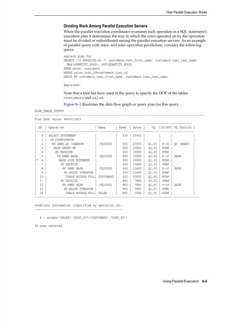
8/16/2019 Oracle Database VLDB and Partitioning Guide
http://slidepdf.com/reader/full/oracle-database-vldb-and-partitioning-guide 211/304
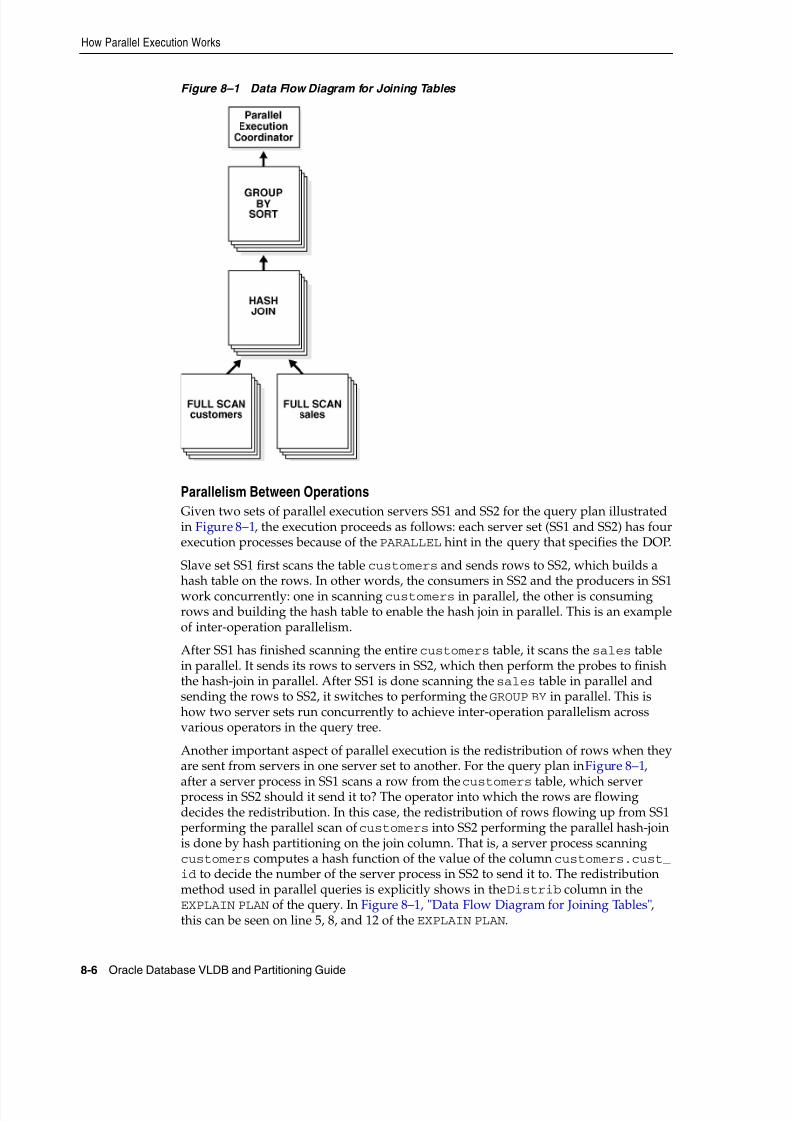
8/16/2019 Oracle Database VLDB and Partitioning Guide
http://slidepdf.com/reader/full/oracle-database-vldb-and-partitioning-guide 212/304
How Parallel Execution Works
8-6 Oracle Database VLDB and Partitioning Guide
Figure 8–1 Data Flow Diagram for Joining Tables
Parallelism Between Operations
Given two sets of parallel execution servers SS1 and SS2 for the query plan illustratedin Figure 8–1, the execution proceeds as follows: each server set (SS1 and SS2) has fourexecution processes because of the PARALLEL hint in the query that specifies the DOP.
Slave set SS1 first scans the table customers and sends rows to SS2, which builds ahash table on the rows. In other words, the consumers in SS2 and the producers in SS1work concurrently: one in scanning customers in parallel, the other is consumingrows and building the hash table to enable the hash join in parallel. This is an exampleof inter-operation parallelism.
After SS1 has finished scanning the entire customers table, it scans the sales tablein parallel. It sends its rows to servers in SS2, which then perform the probes to finishthe hash-join in parallel. After SS1 is done scanning the sales table in parallel andsending the rows to SS2, it switches to performing the GROUP BY in parallel. This ishow two server sets run concurrently to achieve inter-operation parallelism acrossvarious operators in the query tree.
Another important aspect of parallel execution is the redistribution of rows when theyare sent from servers in one server set to another. For the query plan in Figure 8–1,
after a server process in SS1 scans a row from the customers table, which serverprocess in SS2 should it send it to? The operator into which the rows are flowingdecides the redistribution. In this case, the redistribution of rows flowing up from SS1performing the parallel scan of customers into SS2 performing the parallel hash-joinis done by hash partitioning on the join column. That is, a server process scanningcustomers computes a hash function of the value of the column customers.cust_id to decide the number of the server process in SS2 to send it to. The redistributionmethod used in parallel queries is explicitly shows in the Distrib column in theEXPLAIN PLAN of the query. In Figure 8–1, "Data Flow Diagram for Joining Tables",this can be seen on line 5, 8, and 12 of the EXPLAIN PLAN.

8/16/2019 Oracle Database VLDB and Partitioning Guide
http://slidepdf.com/reader/full/oracle-database-vldb-and-partitioning-guide 213/304
How Parallel Execution Works
Using Parallel Execution 8-7
Producer/Consumer Operations
Operations that require the output of other operations are known as consumeroperations. In Figure 8–1, the GROUP BY SORT operation is the consumer of the HASH JOIN operation because GROUP BY SORT requires the HASH JOIN output.
Consumer operations can begin consuming rows as soon as the producer operationshave produced rows. In the previous example, while the parallel execution servers are
producing rows in the FULL SCAN of the sales table, another set of parallel executionservers can begin to perform the HASH JOIN operation to consume the rows.
Each of the two operations performed concurrently is given its own set of parallelexecution servers. Therefore, both query operations and the data flow tree itself haveparallelism. The parallelism of an individual operation is called intra-operationparallelism and the parallelism between operations in a data flow tree is calledinter-operation parallelism. Due to the producer-consumer nature of the Oracledatabase's operations, only two operations in a given tree must be performedsimultaneously to minimize execution time. To illustrate intra- and inter-operationparallelism, consider the following statement:
SELECT * FROM employees ORDER BY last_name;
The execution plan implements a full scan of the employees table. This operation isfollowed by a sorting of the retrieved rows, based on the value of the last_name column. For the sake of this example, assume the last_name column is not indexed.Also assume that the DOP for the query is set to 4, which means that four parallelexecution servers can be active for any given operation.
Figure 8–2 illustrates the parallel execution of the example query.
Figure 8–2 Interoperation Parallelism and Dynamic Partitioning
As you can see from Figure 8–2, there are actually eight parallel execution serversinvolved in the query even though the DOP is 4. This is because a producer andconsumer operator can be performed at the same time (interoperation parallelism).
Also note that all of the parallel execution servers involved in the scan operation sendrows to the appropriate parallel execution server performing the SORT operation. If arow scanned by a parallel execution server contains a value for the last_name
SELECT * from employees ORDER BY last_name;
employees Table
ParallelExecution
Coordinator
T - Z
H - M
N - S
A - G
UserProcess
Parallel executionservers forORDER BYoperation
Parallel executionservers for fulltable scan
Intra-Operationparallelism
Inter-Operationparallelism
Intra-Operationparallelism

8/16/2019 Oracle Database VLDB and Partitioning Guide
http://slidepdf.com/reader/full/oracle-database-vldb-and-partitioning-guide 214/304
How Parallel Execution Works
8-8 Oracle Database VLDB and Partitioning Guide
column between A and G, that row gets sent to the first ORDER BY parallel executionserver. When the scan operation is complete, the sorting processes can return thesorted results to the query coordinator, which, in turn, returns the complete queryresults to the user.
How Parallel Execution Servers Communicate
To execute a query in parallel, Oracle Database generally creates a set of producerparallel execution servers and a set of consumer parallel execution servers. Theproducer server retrieves rows from tables and the consumer server performsoperations such as join, sort, DML, and DDL on these rows. Each server in theproducer set has a connection to each server in the consumer set. The number ofvirtual connections between parallel execution servers increases as the square of thedegree of parallelism.
Each communication channel has at least one, and sometimes up to four memory buffers, which are allocated from the SHARED_POOL. Multiple memory buffersfacilitate asynchronous communication among the parallel execution servers.
A single-instance environment uses at most three buffers for each communicationchannel. An Oracle Real Application Clusters environment uses at most four buffers
for each channel. Figure 8–3 illustrates message buffers and how producer parallelexecution servers connect to consumer parallel execution servers.
Figure 8–3 Parallel Execution Server Connections and Buffers
When a connection is between two processes on the same instance, the serverscommunicate by passing the buffers back and forth in memory (in the SHARED_POOL).When the connection is between processes in different instances, the messages are sent
using external high-speed network protocols over the interconnect. In Figure 8–3, theDOP equals the number of parallel execution servers, which in this case is n.Figure 8–3 does not show the parallel execution coordinator. Each parallel executionserver actually has an additional connection to the parallel execution coordinator. It isimportant to size the SHARED_POOL adequately when using parallel execution. If thereis not enough free space in the SHARED_POOL to allocate the necessary memory buffers for a parallel server, it fails to start.
connections
messagebuffer
DOP = 1 DOP = 2
. . .
. . .
DOP = n
Parallelexecutionserver set 1
Parallelexecution
server set 2
8/16/2019 Oracle Database VLDB and Partitioning Guide
http://slidepdf.com/reader/full/oracle-database-vldb-and-partitioning-guide 215/304
How Parallel Execution Works
Using Parallel Execution 8-9
Degree of ParallelismThe number of parallel execution servers associated with a single operation is knownas the degree of parallelism (DOP). Parallel execution is designed to effectively usemultiple CPUs. Oracle Database's parallel execution framework enables you to eitherexplicitly chose a specific degree of parallelism or to rely on Oracle to automaticallycontrol it.
This section contains the following topics:
■ Manually Specifying the Degree of Parallelism
■ Automatic Parallel Degree Policy
■ Controlling Automatic Degree of Parallelism
■ In-Memory Parallel Execution
■ Adaptive Parallelism
■ Controlling Automatic DOP, Parallel Statement Queuing, and In-Memory ParallelExecution
Manually Specifying the Degree of ParallelismA specific DOP can be requested from the Oracle database. For example, you can set afixed DOP at a table or index level:
ALTER TABLES sales PARALLEL 8;ALTER TABLE customers PARALLEL 4;
In this case, queries accessing just the sales table use a requested DOP of 8 andqueries accessing the customers table request a DOP of 4. A query accessing both thesales and the customers table is processed with a DOP of 8 and potentially allocate16 parallel servers (producer/consumer); whenever different DOPs are specified,Oracle Database uses the higher DOP.
Default Parallelism If the PARALLEL clause is specified but no degree is listed, the objectgets the default DOP. Default parallelism uses a formula to determine the DOP basedon the system configuration, as in the following:
■ For a single instance, DOP = PARALLEL_THREADS_PER_CPU x CPU_COUNT
■ For an Oracle RAC configuration, DOP = PARALLEL_THREADS_PER_CPU xCPU_COUNT x INSTANCE_COUNT
By default, INSTANCE_COUNT is all of the nodes in the cluster. However, if you haveused Oracle RAC services to limit the number of nodes a parallel operation canexecute across, then the number of participating nodes is the number of nodes belonging to that service. For example, on a four node Oracle RAC cluster, with eachnode having 8 CPU cores and no Oracle RAC services, the default DOP would be 2 x 8x 4 = 64.
The default DOP algorithm is designed to use maximum resources and assumes thatthe operation finishes faster if it can use more resources. Default parallelism targets thesingle-user workload. In a multiuser environment, default parallelism is notrecommended.
The DOP for a SQL statement can also be set or limited by the Resource Manager. SeeOracle Database Administrator's Guide for more information.

8/16/2019 Oracle Database VLDB and Partitioning Guide
http://slidepdf.com/reader/full/oracle-database-vldb-and-partitioning-guide 216/304
How Parallel Execution Works
8-10 Oracle Database VLDB and Partitioning Guide
Automatic Parallel Degree Policy
When the parameter PARALLEL_DEGREE_POLICY is set to AUTO, Oracle Databaseautomatically decides if a statement should execute in parallel or not and what DOP itshould use. Oracle Database also determines if the statement can be executedimmediately or if it is queued until more system resources are available. Finally, OracleDatabase decides if the statement can take advantage of the aggregated clustermemory or not.
The following is a summary of parallel statement processing when parallel degreepolicy is set to automatic.
1. A SQL statement is issued.
2. The statement is parsed and the optimizer determines the execution plan.
3. The threshold limit specified by the PARALLEL_MIN_TIME_THRESHOLD initialization parameter is checked.
a. If the execution time is less than the threshold limit, the SQL statement is runserially.
b. If the execution time is greater than the threshold limit, the statement is run in
parallel based on the DOP that the optimizer calculates.For more information, see "Determining Degree of Parallelism" on page 8-10 and"Controlling Automatic Degree of Parallelism" on page 8-11.
Determining Degree of Parallelism The optimizer automatically determines the DOP for astatement based on the resource requirements of the statement. The optimizer uses thecost of all scan operations (full table scan, index fast full scan, and so on) in theexecution plan to determine the necessary DOP for the statement.
However, the optimizer caps the actual DOP to ensure parallel server processes do notflood the system. This cap is set by the parameter PARALLEL_DEGREE_LIMIT. Thedefault for value for this parameter is CPU, which means the number of processes islimited by the number of CPUs on the system (PARALLEL_THREADS_PER_CPU *
CPU_COUNT * INSTANCE_COUNT) also known as the default DOP. By adjusting thisparameter setting, you can control the maximum DOP the optimizer can choose for aSQL statement.
The DOP determined by the optimizer is shown in the notes section of an executionplan, visible either using the explain plan command or V$SQL_PLAN.
EXPLAIN PLAN FORSELECT SUM(AMOUNT_SOLD) FROM SH.SALES;
PLAN TABLE OUTPUT
Plan hash value: 672559287-------------------------------------------------------------------------------------------------| Id | Operation | Name | Rows | Bytes | Cost(%CPU) | Time | Pstart | Pstop |-------------------------------------------------------------------------------------------------| 0 | SELECT STATEMENT | | 1 | 4 | 5 (0) | 00:00:01 | | || 1 | SORT AGGREGATE | | 1 | 4 | | | | || 2 | PX COORDINATOR | | 1 | 4 | | | | || 3 | PX SEND QC(RANDOM) |:TQ10000| 1 | 4 | 5 (0) | | | || 4 | SORT AGGREGATE | | 1 | 4 | | | | || 5 | PX BLOCK ITERATOR | | 960 | 3840 | 5 (0) | 00:00:01 | 1 | 16 || 6 | TABLE ACCESS FULL | SALES | 960 | 3840 | 5 (0) | 00:00:01 | 1 | 16 |--------------------------------------------------------------------------------------------------
8/16/2019 Oracle Database VLDB and Partitioning Guide
http://slidepdf.com/reader/full/oracle-database-vldb-and-partitioning-guide 217/304
How Parallel Execution Works
Using Parallel Execution 8-11
Note----- - Computed Degree of Parallelism is 2 - Degree of Parallelism of 2 is derived from scan of object SH.SALES
PARALLEL_MIN_TIME_THRESHOLD is the second initialization parameter thatcontrols automatic DOP. It specifies the minimum execution time a statement should
have before the statement is considered for automatic DOP. By default, this is 10seconds. The optimizer first calculates a serial execution plan for the SQL statement; ifthe estimated execution elapse time is greater than PARALLEL_MIN_TIME_THRESHOLD (10 seconds), the statement becomes a candidate for automatic DOP.
Controlling Automatic Degree of Parallelism
There are two initialization parameters that control automatic DOP, PARALLEL_DEGREE_POLICY and PARALLEL_MIN_TIME_THRESHOLD. They are described in thissection, and "Automatic Parallel Degree Policy" on page 8-10 and "ControllingAutomatic DOP, Parallel Statement Queuing, and In-Memory Parallel Execution" onpage 8-12.
Setting Automatic Degree of Parallelism Using ALTER SESSION Statements You can set theDOP using an ALTER SESSION statement, as in the following:
ALTER SESSION SET parallel_degree_policy = limited;ALTER TABLE emp parallel (degree default);
Setting Automatic Degree of Parallelism Using Hints You can use the PARALLEL hint to forceparallelism. It takes an optional parameter, the DOP at which the statement shouldrun. In addition, the NO_PARALLEL hint overrides a PARALLEL parameter in the DDLthat created or altered the table.
The following example illustrates forcing the statement to be executed in parallel:
SELECT /*+parallel */ ename, dname FROM emp e, dept d WHERE e.deptno=d.deptno;
The following example illustrates forcing the statement to be executed in parallel witha degree of 10:
SELECT /*+ parallel(10) */ ename, dname FROM emp e, dept d WHERE e.deptno=d.deptno;
The following example illustrates forcing the statement to be executed in serial:
SELECT /*+ no_parallel */ ename, dname FROM emp e, dept d WHERE e.deptno=d.deptno;
The following example illustrates computing the DOP the statement should use:
SELECT /*+ parallel(auto) */ ename, dname FROM emp e, dept d WHERE e.deptno=d.deptno;
The following example forces the statement to use Oracle Database 11 g, Release 1(11.1) behavior:
SELECT /*+ parallel(manual) */ ename, dname FROM emp e, dept d WHERE e.deptno=d.deptno;
In-Memory Parallel Execution
When the parameter PARALLEL_DEGREE_POLICY is set to AUTO, Oracle Databasedecides if an object that is accessed using parallel execution would benefit from being
8/16/2019 Oracle Database VLDB and Partitioning Guide
http://slidepdf.com/reader/full/oracle-database-vldb-and-partitioning-guide 218/304
How Parallel Execution Works
8-12 Oracle Database VLDB and Partitioning Guide
cached in the SGA (buffer cache). The decision to cache an object is based on awell-defined set of heuristics including the size of the object and frequency on which itis accessed. In an Oracle RAC environment, Oracle Database affinitizes or maps piecesof the object into each of the buffer caches on the active instances. By creating thismapping, Oracle Database automatically knows which buffer cache to access to finddifferent parts or pieces of the object. Using this information, Oracle Database preventsmultiple instances from reading the same information from disk over and over again,
thus maximizing the amount of memory that can cache objects. If the size of the objectis larger than the size of the buffer cache (single instance) or the size of the buffer cachemultiplied by the number of active instances in an Oracle RAC cluster, then it is readusing direct path reads.
Adaptive Parallelism
The adaptive multiuser algorithm, which is enabled by default, reduces the degree ofparallelism as the load on the system increases. When using Oracle's adaptiveparallelism capabilities, the database uses an algorithm at SQL execution time todetermine whether a parallel operation should receive the requested DOP or have itsDOP lower to ensure the system is not overloaded.
In a system that makes aggressive use of parallel execution by using a high DOP, theadaptive algorithm adjusts the DOP down with only few operations running inparallel. While the algorithm still ensures optimal resource utilization, users mayexperience inconsistent response times. Using solely the adaptive parallelismcapabilities in an environment that requires deterministic response times is notadvised. Adaptive parallelism is controlled through the database initializationparameter PARALLEL_ADAPTIVE_MULTI_USER.
Controlling Automatic DOP, Parallel Statement Queuing, and In-Memory ParallelExecution
The initialization parameter PARALLEL_DEGREE_POLICY controls whether automaticdegree of parallelism (Auto DOP), parallel statement queuing, and in-memory parallelexecution is enabled. This parameter has three possible values:
■ MANUAL - Disables Auto DOP, statement queuing and in-memory parallelexecution. It reverts the behavior of parallel execution to what it was previous toOracle Database 11 g, Release 2 (11.2), which is the default.
■ LIMITED - Enables Auto DOP for some statements but parallel statement queuingand in-memory parallel execution are disabled. Auto DOP is only applied tostatements that access tables or indexes decorated explicitly with the PARALLEL clause. Tables and indexes that have a specific DOP specified uses that specifiedDOP.
■ AUTO - Enables Auto DOP, parallel statement queuing, and in-memory parallelexecution.
By default, the system only uses parallel execution when a parallel degree has beenexplicitly set on an object or if a parallel hint is specified in the SQL statement. Thedegree of parallelism used is exactly what was specified. No parallel statement queueoccurs and parallel execution does not use the buffer cache. For information about theparallel statement queue, refer to "Parallel Statement Queuing" on page 8-13.
If you want Oracle Database to only automatically decide the degree of parallelism fora subset of SQL statements that touch a specific subset of objects, then set PARALLEL_DEGREE_POLICY to LIMITED and set the parallel clause on that subset of objects. Ifyou want Oracle Database to automatically decide the degree of parallelism, then setPARALLEL_DEGREE_POLICY to AUTO.

8/16/2019 Oracle Database VLDB and Partitioning Guide
http://slidepdf.com/reader/full/oracle-database-vldb-and-partitioning-guide 219/304
How Parallel Execution Works
Using Parallel Execution 8-13
When PARALLEL_DEGREE_POLICY is set to AUTO, Oracle Database determineswhether the statement should run in parallel based on the cost of the operations in theexecution plan and the hardware characteristics. The hardware characteristics includeI/O calibration statistics so these statistics must be gathered otherwise OracleDatabase does not use the automatic degree policy feature.
If I/O calibration is not run to gather the required statistics, the explain plan includes
the following text in its notes:automatic DOP: skipped because of IO calibrate statistics are missing
I/O calibration statistics can be gathered with the PL/SQL DBMS_RESOURCE_MANAGER.CALIBRATE_IO procedure. I/O calibration is a one-time action if thephysical hardware does not change.
Parallel Statement QueuingWhen the parameter PARALLEL_DEGREE_POLICY is set to AUTO, Oracle queues SQLstatements that require parallel execution if the necessary parallel server processes arenot available. After the necessary resources become available, the SQL statement isdequeued and allowed to execute. The default dequeue order is a simple first in, firstout queue based on the time a statement was issued.
The following is a summary of parallel statement processing.
1. A SQL statements is issued.
2. The statement is parsed and the DOP is automatically determined.
3. Available parallel resources are checked.
a. If there are enough parallel resources and there are no statements ahead in thequeue waiting for the resources, the SQL statement is executed.
b. If there are not enough parallel servers, the SQL statement is queued based onspecified conditions and dequeued from the front of the queue when specifiedconditions are met.
Parallel statements are queued if running the statements would increase the number ofactive parallel servers above the value of the PARALLEL_SERVERS_TARGET initialization parameter. For example, if PARALLEL_SERVERS_TARGET is set to 64, thenumber of current active servers is 60, and a new parallel statement needs 16 parallelservers, it would be queued because 16 added to 60 is greater than 64, the value of
PARALLEL_SERVERS_TARGET.By default, the PARALLEL_SERVERS_TARGET parameter is set to 4 x CPU_COUNT xPARALLEL_THREADS_PER_CPU x ACTIVE_INSTANCES. This is not the maximumnumber of parallel server processes allowed on the system, but the number availableto run parallel statements before parallel statement queuing is used. It is set lower thanthe maximum number of parallel server processes allowed on the system (PARALLEL_MAX_SERVERS) to ensure each parallel statement gets all of the parallel serverresources required and to prevent overloading the system with parallel serverprocesses. Note all serial (non-parallel) statements executes immediately even ifparallel statement queuing has been activated.
See Also:
■ Oracle Database Performance Tuning Guide for information aboutI/O calibration
■ Oracle Database PL/SQL Packages and Types Reference forinformation about the DBMS_RESOURCE_MANAGER package
8/16/2019 Oracle Database VLDB and Partitioning Guide
http://slidepdf.com/reader/full/oracle-database-vldb-and-partitioning-guide 220/304
How Parallel Execution Works
8-14 Oracle Database VLDB and Partitioning Guide
If a statement has been queued, it is identified by the resmgr:pq queued wait event.
This section discusses the following topics:
■ Managing Parallel Statement Queuing with Resource Manager
■ Grouping Parallel Statements with a BEGIN_SQL_BLOCK .. END_SQL_BLOCKBlock
■ Managing Parallel Statement Queuing with Hints
Managing Parallel Statement Queuing with Resource Manager
By default, the parallel statement queue operates as a first-in, first-out queue. Byconfiguring and setting a resource plan, you can control the order in which parallelstatements are dequeued and the number of parallel servers used by each workload or
consumer group.Resource plans and consumer groups are created using the DBMS_RESOURCE_MANAGER PL/SQL package. A resource plan consists of a collection of directives foreach consumer group which specify controls and allocations for various databaseresources, such as parallel servers. A resource plan is enabled by setting theRESOURCE_MANAGER_PLAN parameter to the name of the resource plan.
The following sections describe the directives that can be used to manage theprocessing of parallel statements for consumer groups when the parallel degree policyis set to AUTO.
■ Managing the Order of the Parallel Statement Queue
■ Limiting the Parallel Server Resources for a Consumer Group
■ Specifying a Parallel Statement Queue Timeout for Each Consumer Group
■ Specifying a Degree of Parallelism Limit for Consumer Groups
■ A Sample Scenario for Managing Statements in the Parallel Queue
In all cases, the parallel statement queue is managed as a single queue on an OracleRAC database. Limits for each consumer group apply to all sessions across the OracleRAC database that belong to that consumer group. The queuing of parallel statementsoccurs based on the sum of the values of the PARALLEL_SERVERS_TARGET initialization parameter across all database instances.
Note: This functionality is available starting with Oracle Database11g Release 2 (11.2.0.2).
See Also:
■ Oracle Database Administrator's Guide for information aboutmanaging Oracle Database resources with Resource Manager
■ Oracle Database Reference for information about V$RSRC* views,the DBA_HIST_RSRC_CONSUMER_GROUP view, and parallel querywait events
■ Oracle Database PL/SQL Packages and Types Reference forinformation about the DBMS_RESOURCE_MANAGER package

8/16/2019 Oracle Database VLDB and Partitioning Guide
http://slidepdf.com/reader/full/oracle-database-vldb-and-partitioning-guide 221/304
How Parallel Execution Works
Using Parallel Execution 8-15
Managing the Order of the Parallel Statement Queue You can use Resource Manager tomanage the order that parallel statements are dequeued from the parallel statementqueue. The parallel statements for a particular consumer group are always dequeuedin FIFO order. The directives mgmt_p1 ... mgmt_p8 are used to determine whichconsumer group's parallel statement should be dequeued next. These directives areconfigured using the CREATE_PLAN_DIRECTIVE or UPDATE_PLAN_DIRECTIVE procedure in the DBMS_RESOURCE_MANAGER PL/SQL package.
For example, you can create the PQ_HIGH, PQ_MEDIUM, and PQ_LOW consumergroups and map parallel statement sessions to these consumer groups based onpriority. You then create a resource plan that sets mgmt_p1 to 70% for PQ_HIGH, 25%for PQ_MEDIUM, and 5% for PQ_LOW. This indicates that PQ_HIGH statements aredequeued next with a probability of 70% of the time, PQ_MEDIUM dequeued nextwith a probability of 25% of the time, and PQ_LOW dequeued next with a probabilityof 5% of the time.
Limiting the Parallel Server Resources for a Consumer Group You can use Resource Managerto limit the number of parallel servers that parallel statements from lower priorityconsumer groups can use for parallel statement processing. Using Resource Manageryou can map parallel statement sessions to different consumer groups that each have
specific limits on the number of the parallel servers that can be used. When theselimits are specified, parallel statements from a consumer group are queued when thislimit would be exceeded.
This limitation becomes useful when a database has high priority and low priorityconsumer groups. Without limits, a user may issue a large number of parallelstatements from a low-priority consumer group that utilizes all parallel servers. Whena parallel statement from a high priority consumer group is issued, the resourceallocation directives can ensure that the high priority parallel statement is dequeuedfirst. By limiting the number of parallel servers a low-priority consumer group canuse, you can ensure that there are always some parallel servers available for a highpriority consumer group.
To limit the parallel servers used by a consumer group, use the parallel_target_
percentage parameter with the CREATE_PLAN_DIRECTIVE procedure or the new_parallel_target_percentage parameter with the UPDATE_PLAN_DIRECTIVE procedure in the DBMS_RESOURCE_MANAGER package. The parallel_target_percentage and new_parallel_target_percentage parameters specify themaximum percentage of the Oracle RAC-wide parallel server pool that is specified byPARALLEL_SERVERS_TARGET that a consumer group can use.
For example, on an Oracle RAC database system, the initialization parameterPARALLEL_SERVERS_TARGET is set to 32 on two nodes so there are a total of 32 x 2 =64 parallel servers that can be used before queuing begins. You can set up theconsumer group PQ_LOW to use 50% of the available parallel servers (parallel_target_percentage = 50) and low priority statements can then be mapped to thePQ_LOW consumer group. This scenario limits any parallel statements from the PQ_
LOW consumer group to 64 x 50% = 32 parallel servers, even though there are moreinactive or unused parallel servers. In this scenario, after the statements from the PQ_LOW consumer group have used 32 parallel servers, statements from that consumergroup are queued.
It is possible in one database to have some sessions with the parallelism degree policyset to MANUAL and some sessions set to AUTO. In this scenario, only the sessionswith parallelism degree policy set to AUTO can be queued. However, the parallelservers used in sessions where the parallelism degree policy is set to MANUAL areincluded in the total of all parallel servers used by a consumer group.
8/16/2019 Oracle Database VLDB and Partitioning Guide
http://slidepdf.com/reader/full/oracle-database-vldb-and-partitioning-guide 222/304
How Parallel Execution Works
8-16 Oracle Database VLDB and Partitioning Guide
For information about limiting parallel resources for users, refer to "When Users HaveToo Many Processes" on page 8-43 and "Limiting the Number of Resources for a Userusing a Consumer Group" on page 8-44.
Specifying a Parallel Statement Queue Timeout for Each Consumer Group You can useResource Manager to set the maximum queue timeout limit so that parallel statementsdo not stay in the queue for long periods of time. Using Resource Manager you can
map parallel statement sessions to different consumer groups that each have specificmaximum timeout limits in a resource plan.
To manage the queue timeout, the parallel_queue_timeout parameter is usedwith the CREATE_PLAN_DIRECTIVE procedure or the new_parallel_queue_timeout parameter is used with the UPDATE_PLAN_DIRECTIVE procedure in theDBMS_RESOURCE_MANAGER package. The parallel_queue_timeout and new_parallel_queue_timeout parameters specify the time in seconds that a statementcan remain in a consumer group parallel statement queue. After the timeout periodhas expired, the statement is terminated with error ORA-7454 and removed from theparallel statement queue.
Specifying a Degree of Parallelism Limit for Consumer Groups You can use Resource
Manager to the limit the degree of parallelism for specific consumer groups. UsingResource Manager you can map parallel statement sessions to different consumergroups that each have specific limits for the degree of parallelism in a resource plan.
To manage the limit of parallelism in consumer groups, use the parallel_degree_limit_p1 parameter with the CREATE_PLAN_DIRECTIVE procedure in the DBMS_RESOURCE_MANAGER package or the new_parallel_degree_limit_p1 parameterwith the UPDATE_PLAN_DIRECTIVE procedure in the DBMS_RESOURCE_MANAGER package. The parallel_degree_limit_p1 and new_parallel_degree_limit_p1 parameters specify a limit on the degree of parallelism for any operation.
For example, you can create the PQ_HIGH, PQ_MEDIUM, and PQ_LOW consumergroups and map parallel statement sessions to these consumer groups based onpriority. You then create a resource plan that specifies degree of parallelism limits so
that the PQ_HIGH limit is set to 16, the PQ_MEDIUM limit is set to 8, and the PQ_LOW limit is set to 2.
A Sample Scenario for Managing Statements in the Parallel Queue This scenario discusseshow to manage statements in the parallel queue with consumer groups set up withResource Manager. For this scenario, consider a data warehouse workload thatconsists of three types of SQL statements:
■ Short-running SQL statements
Short-running identifies statements running less than one minute. You expectthese statements to have very good response times.
■ Medium-running SQL statements
Medium-running identifies statements running more than one minute, but lessthan 15 minutes. You expect these statements to have reasonably good responsetimes.
■ Long-running SQL statements
Long-running identifies statements that are ad-hoc or complex queries runningmore than 15 minutes. You expect these statements to take a long time.
For this data warehouse workload, you want better response times for theshort-running statements. To achieve this goal, you must ensue that:
8/16/2019 Oracle Database VLDB and Partitioning Guide
http://slidepdf.com/reader/full/oracle-database-vldb-and-partitioning-guide 223/304
How Parallel Execution Works
Using Parallel Execution 8-17
■ Long-running statements do not use all of the parallel server resources, forcingshorter statements to wait in the parallel statement queue.
■ When both short-running and long-running statements are queued, short-runningstatements should be dequeued ahead of long-running statements.
■ The DOP for short-running queries is limited because the speedup from a veryhigh DOP is not significant enough to justify the use of a large number of parallel
servers.
Example 8–1 shows how to set up consumer groups using Resource Manager to setpriorities for statements in the parallel statement queue. Note the following for thisexample:
■ By default, users are assigned to the OTHER_GROUPS consumer group. If theestimated execution time of a SQL statement is longer than 1 minute (60 seconds),then the user switches to MEDIUM_SQL_GROUP. Because switch_for_call isset to TRUE, the user returns to OTHER_GROUPS when the statement hascompleted. If the user is in MEDIUM_SQL_GROUP and the estimated executiontime of the statement is longer than 15 minutes (900 seconds), the user switches toLONG_SQL_GROUP. Similarly, because switch_for_call is set to TRUE, theuser returns to OTHER_GROUPS when the query has completed. The directivesused to accomplish the switch process are switch_time, switch_estimate,switch_for_call, and switch_group.
■ After the number of active parallel servers reaches the value of the PARALLEL_SERVERS_TARGET initialization parameter, subsequent parallel statements arequeued. The mgmt_p[1-8] directives control the order in which parallelstatements are dequeued when parallel servers become available. Because mgmt_p1 is set to 100% for SYS_GROUP in this example, parallel statements from SYS_GROUP are always dequeued first. If no parallel statements from SYS_GROUP arequeued, then parallel statements from OTHER_GROUPS are dequeued withprobability 70%, from MEDIUM_SQL_GROUP with probability 20%, and LONG_SQL_GROUP with probability 10%.
■
Parallel statements issued from OTHER_GROUPS are limited to a DOP of 4 withthe setting of the parallel_degree_limit_p1 directive.
■ To prevent parallel statements of the LONG_SQL_GROUP group from using all ofthe parallel servers, which could potentially cause parallel statements fromOTHER_GROUPS or MEDIUM_SQL_GROUP to wait for long periods of time, itsparallel_target_percentage directive is set to 50%. This means that afterLONG_SQL_GROUP has used up 50% of the parallel servers set with thePARALLEL_SERVERS_TARGET initialization parameter, its parallel statements areforced to wait in the queue.
■ Because parallel statements of the LONG_SQL_GROUP group may be queued fora significant amount of time, a timeout is configured for 14400 seconds (4 hours).When a parallel statement from LONG_SQL_GROUP has waited in the queue for
4 hours, the statement is terminated with the error ORA-7454.
Example 8–1 Using consumer groups to set priorities in the parallel statement queue
BEGIN DBMS_RESOURCE_MANAGER.CREATE_PENDING_AREA(); /* Create consumer groups.
* By default, users start in OTHER_GROUPS, which is automatically * created for every database. */

8/16/2019 Oracle Database VLDB and Partitioning Guide
http://slidepdf.com/reader/full/oracle-database-vldb-and-partitioning-guide 224/304
How Parallel Execution Works
8-18 Oracle Database VLDB and Partitioning Guide
DBMS_RESOURCE_MANAGER.CREATE_CONSUMER_GROUP( 'MEDIUM_SQL_GROUP', 'Medium-running SQL statements, between 1 and 15 minutes. Medium priority.');
DBMS_RESOURCE_MANAGER.CREATE_CONSUMER_GROUP( 'LONG_SQL_GROUP', 'Long-running SQL statements of over 15 minutes. Low priority.'); /* Create a plan to manage these consumer groups */
DBMS_RESOURCE_MANAGER.CREATE_PLAN( 'REPORTS_PLAN', 'Plan for daytime that prioritizes short-running queries'); DBMS_RESOURCE_MANAGER.CREATE_PLAN_DIRECTIVE(
'REPORTS_PLAN', 'SYS_GROUP', 'Directive for sys activity', mgmt_p1 => 100); DBMS_RESOURCE_MANAGER.CREATE_PLAN_DIRECTIVE(
'REPORTS_PLAN', 'OTHER_GROUPS', 'Directive for short-running queries', mgmt_p2 => 70, parallel_degree_limit_p1 => 4, switch_time => 60, switch_estimate => TRUE, switch_for_call => TRUE, switch_group => 'MEDIUM_SQL_GROUP'); DBMS_RESOURCE_MANAGER.CREATE_PLAN_DIRECTIVE(
'REPORTS_PLAN', 'MEDIUM_SQL_GROUP', 'Directive for medium-running queries', mgmt_p2 => 20, parallel_target_percentage => 80, switch_time => 900, switch_estimate => TRUE, switch_for_call => TRUE, switch_group => 'LONG_SQL_GROUP'); DBMS_RESOURCE_MANAGER.CREATE_PLAN_DIRECTIVE(
'REPORTS_PLAN', 'LONG_SQL_GROUP', 'Directive for medium-running queries', mgmt_p2 => 10, parallel_target_percentage => 50,
parallel_queue_timeout => 14400); DBMS_RESOURCE_MANAGER.SUBMIT_PENDING_AREA();
END;/
/* Allow all users to run in these consumer groups */EXEC DBMS_RESOURCE_MANAGER_PRIVS.GRANT_SWITCH_CONSUMER_GROUP( 'public', 'MEDIUM_SQL_GROUP', FALSE); EXEC DBMS_RESOURCE_MANAGER_PRIVS.GRANT_SWITCH_CONSUMER_GROUP( 'public', 'LONG_SQL_GROUP', FALSE);
Grouping Parallel Statements with a BEGIN_SQL_BLOCK .. END_SQL_BLOCK
Block
Often it is important for a report or batch job that consists of multiple parallelstatements to complete as quickly as possible. For example, when many reports arelaunched simultaneously, you may want all of the reports to complete as quickly as
Note: This functionality is available starting with Oracle Database11g Release 2 (11.2.0.2).

8/16/2019 Oracle Database VLDB and Partitioning Guide
http://slidepdf.com/reader/full/oracle-database-vldb-and-partitioning-guide 225/304
How Parallel Execution Works
Using Parallel Execution 8-19
possible. However, you also want some specific reports to complete first, rather thanall reports finishing at the same time.
If a report contains multiple parallel statements and PARALLEL_DEGREE_POLICY isset to AUTO, then each parallel statement may be forced to wait in the queue on a busydatabase. For example, the following steps describe a scenario in SQL statementprocessing:
serial statementparallel query - dop 8 -> wait in queueserial statementparallel query - dop 32 -> wait in queueparallel query - dop 4 -> wait in queue
For a report to be completed quickly, the parallel statements must be grouped toproduce the following behavior:
start SQL blockserial statement
parallel query - dop 8 -> first parallel query: ok to wait in queueserial statementparallel query - dop 32 -> avoid or minimize waitparallel query - dop 4 -> avoid or minimize waitend SQL block
To group the parallel statements, you can use the BEGIN_SQL_BLOCK and END_SQL_BLOCK procedures in the DBMS_RESOURCE_MANAGER PL/SQL package. For eachconsumer group, the parallel statement queue is ordered by the time associated witheach of the consumer group's parallel statements. Typically, the time associated with aparallel statement is the time that the statement was enqueued, which means that thequeue appears to be FIFO. When parallel statements are grouped in a SQL block withthe BEGIN_SQL_BLOCK and END_SQL_BLOCK procedures, the first queued parallelstatement also uses the time that it was enqueued. However, the second and allsubsequent parallel statements receive special treatment and are enqueued using theenqueue time of the first queued parallel statement within the SQL block. With thisfunctionality, the statements frequently move to the front of the parallel statementqueue. This preferential treatment ensures that their wait time is minimized.
Managing Parallel Statement Queuing with Hints
You can use the NO_STATEMENT_QUEUING and STATEMENT_QUEUING hints in SQLstatements to manage parallel statement queuing.
■ NO_STATEMENT_QUEUING
When PARALLEL_DEGREE_POLICY is set to AUTO, this hint enables a statement to bypass the parallel statement queue. For example:
SELECT /* NO_STATEMENT_QUEUING */ emp.last_name, dpt.department_nameFROM employees emp, departments dpt
WHERE emp.department_id = dpt.department_id;
See Also: Oracle Database PL/SQL Packages and Types Reference forinformation about the DBMS_RESOURCE_MANAGER package
8/16/2019 Oracle Database VLDB and Partitioning Guide
http://slidepdf.com/reader/full/oracle-database-vldb-and-partitioning-guide 226/304
How Parallel Execution Works
8-20 Oracle Database VLDB and Partitioning Guide
■ STATEMENT_QUEUING
When PARALLEL_DEGREE_POLICY is not set to AUTO, this hint enables astatement to be delayed and to only run when parallel processes are available torun at the requested DOP. For example:
SELECT /* STATEMENT_QUEUING */ emp.last_name, dpt.department_nameFROM employees emp, departments dpt
WHERE emp.department_id = dpt.department_id;
The Parallel Execution Server PoolWhen an instance starts, Oracle Database creates a pool of parallel execution servers,which are available for any parallel operation. The initialization parameterPARALLEL_MIN_SERVERS specifies the number of parallel execution servers thatOracle Database creates at instance startup.
When executing a parallel operation, the parallel execution coordinator obtainsparallel execution servers from the pool and assigns them to the operation. Ifnecessary, Oracle Database can create additional parallel execution servers for theoperation. These parallel execution servers remain with the operation throughoutexecution. After the statement has been processed completely, the parallel executionservers return to the pool.
If the number of parallel operations increases, Oracle Database creates additionalparallel execution servers to handle incoming requests. However, Oracle Databasenever creates more parallel execution servers for an instance than the value specified by the initialization parameter PARALLEL_MAX_SERVERS.
If the number of parallel operations decreases, Oracle Database terminates any parallelexecution servers that have been idle for a threshold interval. Oracle Database doesnot reduce the size of the pool less than the value of PARALLEL_MIN_SERVERS, nomatter how long the parallel execution servers have been idle.
Processing without Enough Parallel Execution ServersOracle Database can process a parallel operation with fewer than the requestednumber of processes. If all parallel execution servers in the pool are occupied and themaximum number of parallel execution servers has been started, the parallel executioncoordinator switches to serial processing.
See Oracle Database Reference for information about using the initialization parameterPARALLEL_MIN_PERCENT and "Tuning General Parameters for Parallel Execution" onpage 8-42 for information about the PARALLEL_MIN_PERCENT and PARALLEL_MAX_SERVERS initialization parameters.
Granules of Parallelism
The basic unit of work in parallelism is a called a granule. Oracle Database divides theoperation being parallelized (for example, a table scan, table update, or index creation)into granules. Parallel execution processes execute the operation one granule at a time.The number of granules and their size correlates with the degree of parallelism (DOP).It also affects how well the work is balanced across query server processes.
Block Range Granules
Block range granules are the basic unit of most parallel operations, even on partitionedtables. Therefore, from an Oracle Database perspective, the degree of parallelism is notrelated to the number of partitions.

8/16/2019 Oracle Database VLDB and Partitioning Guide
http://slidepdf.com/reader/full/oracle-database-vldb-and-partitioning-guide 227/304
How Parallel Execution Works
Using Parallel Execution 8-21
Block range granules are ranges of physical blocks from a table. Oracle Databasecomputes the number and the size of the granules during run-time to optimize and balance the work distribution for all affected parallel execution servers. The numberand size of granules are dependent upon the size of the object and the DOP. Blockrange granules do not depend on static preallocation of tables or indexes. During thecomputation of the granules, Oracle Database takes the DOP into account and tries toassign granules from different data files to each of the parallel execution servers to
avoid contention whenever possible. Additionally, Oracle Database considers the diskaffinity of the granules on MPP systems to take advantage of the physical proximity between parallel execution servers and disks.
Partition Granules
When partition granules are used, a parallel server process works on an entirepartition or subpartition of a table or index. Because partition granules are staticallydetermined by the structure of the table or index when a table or index is created,partition granules do not give you the flexibility in parallelizing an operation that block granules do. The maximum allowable DOP is the number of partitions. Thismight limit the utilization of the system and the load balancing across parallelexecution servers.
When partition granules are used for parallel access to a table or index, you should usea relatively large number of partitions (ideally, three times the DOP), so that OracleDatabase can effectively balance work across the query server processes.
Partition granules are the basic unit of parallel index range scans, joins between twoequipartitioned tables where the query optimizer has chosen to use partition-wise joins, and of parallel operations that modify multiple partitions of a partitioned object.These operations include parallel creation of partitioned indexes, and parallel creationof partitioned tables.
You can tell which types of granules were used by looking at the execution plan of astatement. The line PX BLOCK ITERATOR above the table or index access indicates that block range granules have been used. In the following example plan, you can see this
on line 7 of the execution plan just above the TABLE FULL ACCESS on the SALES table.-------------------------------------------------------------------------------------------------|Id| Operation | Name |Rows|Bytes|Cost%CPU| Time |Pst|Pst| TQ |INOUT|PQDistri|-------------------------------------------------------------------------------------------------| 0|SELECT STATEMENT | | 17| 153 |565(100)|00:00:07| | | | | || 1| PX COORDINATOR | | | | | | | | | | || 2| PX SEND QC(RANDOM) |:TQ10001| 17| 153 |565(100)|00:00:07| | |Q1,01|P->S |QC(RAND)|| 3| HASH GROUP BY | | 17| 153 |565(100)|00:00:07| | |Q1,01|PCWP | || 4| PX RECEIVE | | 17| 153 |565(100)|00:00:07| | |Q1,01|PCWP | || 5| PX SEND HASH |:TQ10000| 17| 153 |565(100)|00:00:07| | |Q1,00|P->P | HASH || 6| HASH GROUP BY | | 17| 153 |565(100)|00:00:07| | |Q1,00|PCWP | || 7| PX BLOCK ITERATOR | | 10M| 85M | 60(97) |00:00:01| 1 | 16|Q1,00|PCWC | ||*8| TABLE ACCESS FULL| SALES | 10M| 85M | 60(97) |00:00:01| 1 | 16|Q1,00|PCWP | |-------------------------------------------------------------------------------------------------
Predicate Information (identified by operation id):---------------------------------------------------8 - filter("CUST_ID"<=22810 AND "CUST_ID">=22300)
When partition granules are used, you see the line PX PARTITION RANGE above thetable or index access in the execution plan. In the example below, on line 6, it says PX PARTITION RANGE ALL because this statement accesses all of the 16 partitions in thetable. If not all of the partitions are accessed, it simply shows PX PARTITION RANGE.
---------------------------------------------------------------------------------------------------

8/16/2019 Oracle Database VLDB and Partitioning Guide
http://slidepdf.com/reader/full/oracle-database-vldb-and-partitioning-guide 228/304
8/16/2019 Oracle Database VLDB and Partitioning Guide
http://slidepdf.com/reader/full/oracle-database-vldb-and-partitioning-guide 229/304
Types of Parallelism
Using Parallel Execution 8-23
Parallel Execution Using Oracle RACBy default, in an Oracle RAC environment, a SQL statement executed in parallel canrun across all of the nodes in the cluster. For this cross-node or inter-node parallelexecution to perform the interconnect in the Oracle RAC environment must be sizeappropriately as inter-node parallel execution may result in a lot of interconnect traffic.If interconnect has a considerably lower bandwidth in comparison to the I/O
bandwidth from the server to the storage subsystem, it may be better to restrict theparallel execution to a single node or to a limited number of nodes. Inter-node parallelexecution does not scale with an undersized interconnect.
To limit inter-node parallel execution, you can control parallel execution in an OracleRAC environment using the PARALLEL_FORCE_LOCAL initialization parameter. Bysetting this parameter to TRUE, the parallel server processes can only execute on thesame Oracle RAC node where the SQL statement was started.
Limiting the Number of Available Instances
In Oracle Real Application Clusters, services are used to limit the number of instancesthat participate in a parallel SQL operation. The default service includes all availableinstances. You can create any number of services, each consisting of one or more
instances. Parallel execution servers are only be used on instances which are membersof the specified service. See Oracle Real Application Clusters Administration andDeployment Guide for more information about instance groups.
Types of ParallelismThis section discusses the types of parallelism in the following topics:
■ About Parallel Queries
■ About Parallel DDL Statements
■ About Parallel DML Operations
■
About Parallel Execution of Functions■ About Other Types of Parallelism
About Parallel QueriesYou can use parallel queries and parallel subqueries in SELECT statements. You canalso parallelize the query portions of DDL statements and DML statements (INSERT,UPDATE, and DELETE). You can also query external tables in parallel.
Parallelization has two components: the decision to parallelize and the degree ofparallelism (DOP). These components are determined differently for queries, DDLoperations, and DML operations. To determine the DOP, Oracle Database looks at thereference objects:
■ Parallel query looks at each table and index, in the portion of the query beingparallelized, to determine which is the reference table. The basic rule is to pick thetable or index with the largest DOP.
■ For parallel DML (INSERT, UPDATE, MERGE, and DELETE), the reference objectthat determines the DOP is the table being modified by and insert, update, ordelete operation. Parallel DML also adds some limits to the DOP to preventdeadlock. If the parallel DML statement includes a subquery, the subquery's DOPis equivalent to the DML operation.
8/16/2019 Oracle Database VLDB and Partitioning Guide
http://slidepdf.com/reader/full/oracle-database-vldb-and-partitioning-guide 230/304
Types of Parallelism
8-24 Oracle Database VLDB and Partitioning Guide
■ For parallel DDL, the reference object that determines the DOP is the table, index,or partition being created, rebuilt, split, or moved. If the parallel DDL statementincludes a subquery, the subquery's DOP is equivalent to the DDL operation.
For information about the query operations that Oracle Database can parallelize, referto "Operations That Can Be Parallelized". For an explanation of how the processesperform parallel queries, refer to "Parallelizing SQL Statements". For examples of
queries that reference a remote object, refer to "Distributed Transaction Restrictions".For information about the conditions for parallelizing a query and the factors thatdetermine the DOP, refer to "Rules for Parallelizing Queries".
Parallel Queries on Index-Organized Tables
The following parallel scan methods are supported on index-organized tables:
■ Parallel fast full scan of a nonpartitioned index-organized table
■ Parallel fast full scan of a partitioned index-organized table
■ Parallel index range scan of a partitioned index-organized table
These scan methods can be used for index-organized tables with overflow areas andfor index-organized tables that contain LOBs.
Nonpartitioned Index-Organized Tables
Parallel query on a nonpartitioned index-organized table uses parallel fast full scan.The DOP is determined, in decreasing order of priority, by:
1. A PARALLEL hint (if present)
2. An ALTER SESSION FORCE PARALLEL QUERY statement
3. The parallel degree associated with the table, if the parallel degree is specified inthe CREATE TABLE or ALTER TABLE statement
The allocation of work is done by dividing the index segment into a sufficiently largenumber of block ranges and then assigning the block ranges to parallel execution
servers in a demand-driven manner. The overflow blocks corresponding to any roware accessed in a demand-driven manner only by the process, which owns that row.
Partitioned Index-Organized Tables
Both index range scan and fast full scan can be performed in parallel. For parallel fastfull scan, parallelization is the same as for nonpartitioned index-organized tables. For aparallel index range scan on a partitioned index-organized table, the DOP is theminimum of the degree picked up from the previous priority list (like in parallel fastfull scan) and the number of partitions in the index-organized table. Depending on theDOP, each parallel execution server gets one or more partitions, each of which containsthe primary key index segment and the associated overflow segment, if any.
Parallel Queries on Object TypesParallel queries can be performed on object type tables and tables containing objecttype columns. Parallel query for object types supports all of the features that areavailable for sequential queries on object types, including:
■ Methods on object types
■ Attribute access of object types
■ Constructors to create object type instances
■ Object views
8/16/2019 Oracle Database VLDB and Partitioning Guide
http://slidepdf.com/reader/full/oracle-database-vldb-and-partitioning-guide 231/304
Types of Parallelism
Using Parallel Execution 8-25
■ PL/SQL and OCI queries for object types
There are no limitations on the size of the object types for parallel queries.
The following restrictions apply to using parallel query for object types.
■ A MAP function is needed to parallelize queries involving joins and sorts (throughORDER BY, GROUP BY, or set operations). Without a MAP function, the query is
automatically executed serially.■ Parallel DML and parallel DDL are not supported with object types, and such
statements are always performed serially.
In all cases where the query cannot execute in parallel because of any of theserestrictions, the whole query executes serially without giving an error message.
Rules for Parallelizing Queries
This section discusses some rules for parallelizing queries.
Decision to Parallelize A SELECT statement can be parallelized only if the followingconditions are satisfied:
■ The query includes a parallel hint specification (PARALLEL or PARALLEL_INDEX)or the schema objects referred to in the query have a PARALLEL declarationassociated with them.
■ At least one table specified in the query requires one of the following:
– A full table scan
– An index range scan spanning multiple partitions
■ No scalar subqueries are in the SELECT list.
Degree of Parallelism The DOP for a query is determined by the following rules:
■ The query uses the maximum DOP taken from all of the table declarations
involved in the query and all of the potential indexes that are candidates to satisfythe query (the reference objects). That is, the table or index that has the greatestDOP determines the query's DOP maximum query directive.
■ If a table has both a parallel hint specification in the query and a paralleldeclaration in its table specification, the hint specification takes precedence overparallel declaration specification. See Table 8–2 on page 8-40 for precedence rules.
About Parallel DDL StatementsThis section includes the following topics on parallelism for DDL statements:
■ DDL Statements That Can Be Parallelized
■ CREATE TABLE ... AS SELECT in Parallel
■ Recoverability and Parallel DDL
■ Space Management for Parallel DDL
DDL Statements That Can Be Parallelized
You can parallelize DDL statements for tables and indexes that are nonpartitioned orpartitioned. Table 8–2 on page 8-40 summarizes the operations that can be parallelizedin DDL statements.
The parallel DDL statements for nonpartitioned tables and indexes are:
8/16/2019 Oracle Database VLDB and Partitioning Guide
http://slidepdf.com/reader/full/oracle-database-vldb-and-partitioning-guide 232/304
Types of Parallelism
8-26 Oracle Database VLDB and Partitioning Guide
■ CREATE INDEX
■ CREATE TABLE ... AS SELECT
■ ALTER INDEX ... REBUILD
The parallel DDL statements for partitioned tables and indexes are:
■ CREATE INDEX
■ CREATE TABLE ... AS SELECT
■ ALTER TABLE ... [MOVE|SPLIT|COALESCE] PARTITION
■ ALTER INDEX ... [REBUILD|SPLIT] PARTITION
■ This statement can be executed in parallel only if the (global) index partition being split is usable.
All of these DDL operations can be performed in no-logging mode for either parallelor serial execution.
CREATE TABLE for an index-organized table can be parallelized either with or withoutan AS SELECT clause.
Different parallelism is used for different operations (see Table 8–2 on page 8-40).Parallel CREATE TABLE ... AS SELECT statements on partitioned tables and parallelCREATE INDEX statements on partitioned indexes execute with a DOP equal to thenumber of partitions.
Parallel DDL cannot occur on tables with object columns. Parallel DDL cannot occuron nonpartitioned tables with LOB columns.
CREATE TABLE ... AS SELECT in Parallel
Parallel execution lets you parallelize the query and create operations of creating atable as a subquery from another table or set of tables. This can be extremely useful inthe creation of summary or rollup tables.
Clustered tables cannot be created and populated in parallel.Figure 8–4 illustrates creating a table from a subquery in parallel.

8/16/2019 Oracle Database VLDB and Partitioning Guide
http://slidepdf.com/reader/full/oracle-database-vldb-and-partitioning-guide 233/304
Types of Parallelism
Using Parallel Execution 8-27
Figure 8–4 Creating a Summary Table in Parallel
Recoverability and Parallel DDL
Parallel DDL is often used to create summary tables or do massive data loads that arestandalone transaction, which do not always need to be recoverable. By switching offOracle Database logging, no undo or redo is generated, so the parallel DML operationis likely to perform better but becomes an all or nothing operation. In other words, ifthe operation fails, for whatever reason, you must completely redo the operation, it isnot possible to restart it.
If you disable logging during parallel table creation (or any other parallel DDL
operation), you should back up the tablespace containing the table after the table iscreated to avoid loss of the table due to media failure.
Use the NOLOGGING clause of the CREATE TABLE, CREATE INDEX, ALTER TABLE, andALTER INDEX statements to disable undo and redo log generation.
Space Management for Parallel DDL
Creating a table or index in parallel has space management implications that affect both the storage space required during a parallel operation and the free space availableafter a table or index has been created.
Storage Space When Using Dictionary-Managed Tablespaces
When creating a table or index in parallel, each parallel execution server uses thevalues in the STORAGE clause of the CREATE statement to create temporary segmentsto store the rows. Therefore, a table created with a NEXT setting of 4 MB and aPARALLEL DEGREE of 16 consumes at least 64 megabytes (MB) of storage during tablecreation because each parallel server process starts with an extent of 4 MB. When theparallel execution coordinator combines the segments, some segments may betrimmed, and the resulting table may be smaller than the requested 64 MB.
CREATE TABLE summary (C1, AVGC2, SUMC3)PARALLEL 5AS
SELECTC1, AVG(C2), SUM(C3)FROM DAILY_SALESGROUP BY (C1);
DAILY_SALESTable
SUMMARYTable
Parallel ExecutionCoordinator
Parallel ExecutionServers
Parallel ExecutionServers
8/16/2019 Oracle Database VLDB and Partitioning Guide
http://slidepdf.com/reader/full/oracle-database-vldb-and-partitioning-guide 234/304
Types of Parallelism
8-28 Oracle Database VLDB and Partitioning Guide
Free Space and Parallel DDL
When you create indexes and tables in parallel, each parallel execution server allocatesa new extent and fills the extent with the table or index data. Thus, if you create anindex with a DOP of 4, the index has at least four extents initially. This allocation ofextents is the same for rebuilding indexes in parallel and for moving, splitting, orrebuilding partitions in parallel.
Serial operations require the schema object to have at least one extent. Parallelcreations require that tables or indexes have at least as many extents as there areparallel execution servers creating the schema object.
When you create a table or index in parallel, it is possible to create pockets of freespace. This occurs when the temporary segments used by the parallel executionservers are larger than what is needed to store the rows.
■ If the unused space in each temporary segment is larger than the value of theMINIMUM EXTENT parameter set at the tablespace level, then Oracle Databasetrims the unused space when merging rows from all of the temporary segmentsinto the table or index. The unused space is returned to the system free space andcan be allocated for new extents, but it cannot be coalesced into a larger segment because it is not contiguous space (external fragmentation).
■ If the unused space in each temporary segment is smaller than the value of theMINIMUM EXTENT parameter, then unused space cannot be trimmed when therows in the temporary segments are merged. This unused space is not returned tothe system free space; it becomes part of the table or index (internal fragmentation)and is available only for subsequent inserts or for updates that require additionalspace.
For example, if you specify a DOP of 3 for a CREATE TABLE ... AS SELECT statement, but there is only one data file in the tablespace, then internal fragmentation may occur,as shown in Figure 8–5 on page 8-29. The pockets of free space within the internal tableextents of a data file cannot be coalesced with other free space and cannot be allocatedas extents.
See Oracle Database Performance Tuning Guide for more information about creatingtables and indexes in parallel.

8/16/2019 Oracle Database VLDB and Partitioning Guide
http://slidepdf.com/reader/full/oracle-database-vldb-and-partitioning-guide 235/304
Types of Parallelism
Using Parallel Execution 8-29
Figure 8–5 Unusable Free Space (Internal Fragmentation)
Rules for DDL Statements
You must keep the following in mind when parallelizing DDL statements.
Decision to Parallelize DDL operations can be parallelized if a PARALLEL clause (declaration) is specified in the syntax. For CREATE INDEX and ALTER INDEX ...REBUILD or ALTER INDEX ... REBUILD PARTITION, the parallel declaration is storedin the data dictionary.
You can use the ALTER SESSION FORCE PARALLEL DDL statement to override theparallel clauses of subsequent DDL statements in a session.
Degree of Parallelism The DOP is determined by the specification in the PARALLEL clause, unless it is overridden by an ALTER SESSION FORCE PARALLEL DDL statement. A rebuild of a partitioned index is never parallelized.
Parallel clauses in CREATE TABLE and ALTER TABLE statements specify tableparallelism. If a parallel clause exists in a table definition, it determines the parallelism
of DDL statements and queries. If the DDL statement contains explicit parallel hintsfor a table, however, those hints override the effect of parallel clauses for that table.You can use the ALTER SESSION FORCE PARALLEL DDL statement to override parallelclauses.
Rules for [CREATE | REBUILD] INDEX or [MOVE | SPLIT] PARTITION
The following rules apply:
DATA1.ORA
CREATE TABLE emp AS SELECT ...
USERS Tablespace
EXTENT 1
Free spacefor INSERTs
Free spacefor INSERTs
Free space
EXTENT 2
EXTENT 3
for INSERTs
ParallelExecution
Server
ParallelExecution
Server
ParallelExecution
Server
8/16/2019 Oracle Database VLDB and Partitioning Guide
http://slidepdf.com/reader/full/oracle-database-vldb-and-partitioning-guide 236/304
Types of Parallelism
8-30 Oracle Database VLDB and Partitioning Guide
Parallel CREATE INDEX or ALTER INDEX ... REBUILD The CREATE INDEX and ALTER INDEX ... REBUILD statements can be parallelized only by a PARALLEL clause or an ALTER SESSION FORCE PARALLEL DDL statement.
ALTER INDEX ... REBUILD can be parallelized only for a nonpartitioned index, butALTER INDEX ... REBUILD PARTITION can be parallelized by a PARALLEL clause oran ALTER SESSION FORCE PARALLEL DDL statement.
The scan operation for ALTER INDEX ... REBUILD (nonpartitioned), ALTER INDEX ...REBUILD PARTITION, and CREATE INDEX has the same parallelism as the REBUILD or CREATE operation and uses the same DOP. If the DOP is not specified for REBUILD or CREATE, the default is the number of CPUs.
Parallel MOVE PARTITION or SPLIT PARTITION The ALTER INDEX ... MOVE PARTITION and ALTER INDEX ...SPLIT PARTITION statements can be parallelized only by aPARALLEL clause or an ALTER SESSION FORCE PARALLEL DDL statement. Their scanoperations have the same parallelism as the corresponding MOVE or SPLIT operations.If the DOP is not specified, the default is the number of CPUs.
Rules for CREATE TABLE AS SELECT
The CREATE TABLE ... AS SELECT statement contains two parts: a CREATE part (DDL)and a SELECT part (query). Oracle Database can parallelize both parts of thestatement. The CREATE part follows the same rules as other DDL operations.
Decision to Parallelize (Query Part) The query part of a CREATE TABLE ... AS SELECT statement can be parallelized only if the following conditions are satisfied:
■ The query includes a parallel hint specification (PARALLEL or PARALLEL_INDEX)or the CREATE part of the statement has a PARALLEL clause specification or theschema objects referred to in the query have a PARALLEL declaration associatedwith them.
■ At least one table specified in the query requires either a full table scan or an indexrange scan spanning multiple partitions.
Degree of Parallelism (Query Part) The DOP for the query part of a CREATE TABLE ... AS SELECT statement is determined by one of the following rules:
■ The query part uses the values specified in the PARALLEL clause of the CREATE part.
■ If the PARALLEL clause is not specified, the default DOP is the number of CPUs.
■ If the CREATE is serial, then the DOP is determined by the query.
Note that any values specified in a hint for parallelism are ignored.
Decision to Parallelize (CREATE Part) The CREATE operation of CREATE TABLE ... AS SELECT can be parallelized only by a PARALLEL clause or an ALTER SESSION FORCE PARALLEL DDL statement.
When the CREATE operation of CREATE TABLE ... AS SELECT is parallelized, OracleDatabase also parallelizes the scan operation if possible. The scan operation cannot beparallelized if, for example:
■ The SELECT clause has a NO_PARALLEL hint
■ The operation scans an index of a nonpartitioned table
8/16/2019 Oracle Database VLDB and Partitioning Guide
http://slidepdf.com/reader/full/oracle-database-vldb-and-partitioning-guide 237/304
Types of Parallelism
Using Parallel Execution 8-31
When the CREATE operation is not parallelized, the SELECT can be parallelized if ithas a PARALLEL hint or if the selected table (or partitioned index) has a paralleldeclaration.
Degree of Parallelism (CREATE Part) The DOP for the CREATE operation, and for theSELECT operation if it is parallelized, is specified by the PARALLEL clause of theCREATE statement, unless it is overridden by an ALTER SESSION FORCE PARALLEL
DDL statement. If the PARALLEL clause does not specify the DOP, the default is thenumber of CPUs.
About Parallel DML OperationsParallel DML (PARALLEL INSERT, UPDATE, DELETE, and MERGE) uses parallelexecution mechanisms to speed up or scale up large DML operations against largedatabase tables and indexes.
This section discusses the following parallel DML topics:
■ When to Use Parallel DML
■ Enabling Parallel DML
■ Transaction Restrictions for Parallel DML
■ Rollback Segments
■ Recovery for Parallel DML
■ Space Considerations for Parallel DML
■ Restrictions on Parallel DML
When to Use Parallel DML
Parallel DML is useful in a DSS environment where the performance and scalability ofaccessing large objects are important. Parallel DML complements parallel query inproviding you with both querying and updating capabilities for your DSS databases.
The overhead of setting up parallelism makes parallel DML operations infeasible forshort OLTP transactions. However, parallel DML operations can speed up batch jobsrunning in an OLTP database.
Several scenarios where parallel DML is used include:
■ Refreshing Tables in a Data Warehouse System
■ Creating Intermediate Summary Tables
■ Using Scoring Tables
■ Updating Historical Tables
■ Running Batch Jobs
Refreshing Tables in a Data Warehouse System In a data warehouse system, large tablesmust be refreshed (updated) periodically with new or modified data from theproduction system. You can do this efficiently by using the MERGE statement.
Note: Although DML generally includes queries, in this chapterthe term DML refers only to inserts, updates, merges, and deletes.
8/16/2019 Oracle Database VLDB and Partitioning Guide
http://slidepdf.com/reader/full/oracle-database-vldb-and-partitioning-guide 238/304
Types of Parallelism
8-32 Oracle Database VLDB and Partitioning Guide
Creating Intermediate Summary Tables In a DSS environment, many applications requirecomplex computations that involve constructing and manipulating many largeintermediate summary tables. These summary tables are often temporary andfrequently do not need to be logged. Parallel DML can speed up the operations againstthese large intermediate tables. One benefit is that you can put incremental results inthe intermediate tables and perform parallel update.
In addition, the summary tables may contain cumulative or comparison informationwhich has to persist beyond application sessions; thus, temporary tables are notfeasible. Parallel DML operations can speed up the changes to these large summarytables.
Using Scoring Tables Many DSS applications score customers periodically based on a setof criteria. The scores are usually stored in large DSS tables. The score information isthen used in making a decision, for example, inclusion in a mailing list.
This scoring activity queries and updates a large number of rows in the table. ParallelDML can speed up the operations against these large tables.
Updating Historical Tables Historical tables describe the business transactions of anenterprise over a recent time interval. Periodically, the DBA deletes the set of oldestrows and inserts a set of new rows into the table. Parallel INSERT ... SELECT andparallel DELETE operations can speed up this rollover task.
Dropping a partition can also be used to delete old rows. However, the table has to bepartitioned by date and with the appropriate time interval.
Running Batch Jobs Batch jobs executed in an OLTP database during off hours have afixed time window in which the jobs must complete. A good way to ensure timely jobcompletion is to parallelize their operations. As the work load increases, morecomputer resources can be added; the scaleup property of parallel operations ensuresthat the time constraint can be met.
Enabling Parallel DML
A DML statement can be parallelized only if you have explicitly enabled parallel DMLin the session. For example, the following statement:
ALTER SESSION ENABLE PARALLEL DML;
This mode is required because parallel DML and serial DML have different locking,transaction, and disk space requirements and parallel DML is disabled for a session bydefault.
When parallel DML is disabled, no DML is executed in parallel even if the PARALLEL hint is used.
When parallel DML is enabled in a session, all DML statements in this session areconsidered for parallel execution. However, even if parallel DML is enabled, the DML
operation may still execute serially if there are no parallel hints or no tables with aparallel attribute or if restrictions on parallel operations are violated.
The session's PARALLEL DML mode does not influence the parallelism of SELECT statements, DDL statements, and the query portions of DML statements. Thus, if thismode is not set, the DML operation is not parallelized, but scans or join operationswithin the DML statement may still be parallelized.
For more information, refer to "Space Considerations for Parallel DML" on page 8-36 and "Restrictions on Parallel DML" on page 8-36.

8/16/2019 Oracle Database VLDB and Partitioning Guide
http://slidepdf.com/reader/full/oracle-database-vldb-and-partitioning-guide 239/304
Types of Parallelism
Using Parallel Execution 8-33
Rules for UPDATE, MERGE, and DELETE
You have two ways to specify parallel directives for UPDATE, MERGE, and DELETE operations (if PARALLEL DML mode is enabled):
■ Use a parallel clause in the definition of the table being updated or deleted (thereference object).
■ Use an update, merge, or delete parallel hint in the statement.
Parallel hints are placed immediately after the UPDATE, MERGE, or DELETE keywordsin UPDATE, MERGE, and DELETE statements. The hint also applies to the underlyingscan of the table being changed.
You can use the ALTER SESSION FORCE PARALLEL DML statement to override parallelclauses for subsequent UPDATE, MERGE, and DELETE statements in a session. Parallelhints in UPDATE, MERGE, and DELETE statements override the ALTER SESSION FORCE PARALLEL DML statement.
For possible limitations, see "Limitation on the Degree of Parallelism" on page 8-60.
Decision to Parallelize The following rule determines whether the UPDATE, MERGE, orDELETE operation should be parallelized:
The UPDATE or DELETE operation is parallelized if and only if at least one of thefollowing is true:
■ The table being updated or deleted has a PARALLEL specification.
■ The PARALLEL hint is specified in the DML statement.
■ An ALTER SESSION FORCE PARALLEL DML statement has been issued previouslyduring the session.
If the statement contains subqueries or updatable views, then they may have their ownseparate parallel hints or clauses. However, these parallel directives do not affect thedecision to parallelize the UPDATE, MERGE, or DELETE.
The parallel hint or clause on the tables is used by both the query and the UPDATE,MERGE, DELETE portions to determine parallelism, the decision to parallelize theUPDATE, MERGE, or DELETE portion is made independently of the query portion, andvice versa.
Degree of Parallelism The DOP is determined by the same rules as for the queries. Notethat, for UPDATE and DELETE operations, only the target table to be modified (the onlyreference object) is involved. Thus, the UPDATE or DELETE parallel hint specificationtakes precedence over the parallel declaration specification of the target table. In otherwords, the precedence order is: MERGE, UPDATE, DELETE hint > Session > Paralleldeclaration specification of target table. See Table 8–2 on page 8-40 for precedencerules.
If the DOP is less than the number of partitions, then the first process to finish work on
one partition continues working on another partition, and so on until the work isfinished on all partitions. If the DOP is greater than the number of partitions involvedin the operation, then the excess parallel execution servers have no work to do.
Example 8–2 Parallelization: Example 1
UPDATE tbl_1 SET c1=c1+1 WHERE c1>100;
8/16/2019 Oracle Database VLDB and Partitioning Guide
http://slidepdf.com/reader/full/oracle-database-vldb-and-partitioning-guide 240/304
Types of Parallelism
8-34 Oracle Database VLDB and Partitioning Guide
If tbl_1 is a partitioned table and its table definition has a parallel clause, then theupdate operation is parallelized even if the scan on the table is serial (such as an indexscan), if the table has multiple partitions with c1 greater than 100.
Example 8–3 Parallelization: Example 2
UPDATE /*+ PARALLEL(tbl_2,4) */ tbl_2 SET c1=c1+1;
Both the scan and update operations on tbl_2 are parallelized with degree four.
Rules for INSERT ... SELECT
An INSERT ... SELECT statement parallelizes its INSERT and SELECT operationsindependently, except for the DOP.
You can specify a parallel hint after the INSERT keyword in an INSERT ... SELECT statement. Because the tables being queried are usually different than the table beinginserted into, the hint enables you to specify parallel directives specifically for theinsert operation.
You have the following ways to specify parallel directives for an INSERT ... SELECT statement (if PARALLEL DML mode is enabled):
■ SELECT parallel hints specified at the statement
■ Parallel clauses specified in the definition of tables being selected
■ INSERT parallel hint specified at the statement
■ Parallel clause specified in the definition of tables being inserted into
You can use the ALTER SESSION FORCE PARALLEL DML statement to override parallelclauses for subsequent INSERT operations in a session. Parallel hints in insertoperations override the ALTER SESSION FORCE PARALLEL DML statement.
Decision to Parallelize The following rule determines whether the INSERT operationshould be parallelized in an INSERT ... SELECT statement:
The INSERT operation is parallelized if and only if at least one of the following is true:
■ The PARALLEL hint is specified after the INSERT in the DML statement.
■ The table being inserted into (the reference object) has a PARALLEL declarationspecification.
■ An ALTER SESSION FORCE PARALLEL DML statement has been issued previouslyduring the session.
The decision to parallelize the INSERT operation is made independently of theSELECT operation, and vice versa.
Degree of Parallelism After the decision to parallelize the SELECT or INSERT operation
is made, one parallel directive is picked for deciding the DOP of the whole statement,using the following precedence rule Insert hint directive > Session> Paralleldeclaration specification of the inserting table > Maximum query directive.
In this context, maximum query directive means that among multiple tables andindexes, the table or index that has the maximum DOP determines the parallelism forthe query operation.
The chosen parallel directive is applied to both the SELECT and INSERT operations.
8/16/2019 Oracle Database VLDB and Partitioning Guide
http://slidepdf.com/reader/full/oracle-database-vldb-and-partitioning-guide 241/304
Types of Parallelism
Using Parallel Execution 8-35
Example 8–4 Parallelization: Example 3
The DOP used is 2, as specified in the INSERT hint:
INSERT /*+ PARALLEL(tbl_ins,2) */ INTO tbl_insSELECT /*+ PARALLEL(tbl_sel,4) */ * FROM tbl_sel;
Transaction Restrictions for Parallel DML
To execute a DML operation in parallel, the parallel execution coordinator acquiresparallel execution servers, and each parallel execution server executes a portion of thework under its own parallel process transaction.
■ Each parallel execution server creates a different parallel process transaction.
■ If you use rollback segments instead of Automatic Undo Management, you maywant to reduce contention on the rollback segments by limiting the number ofparallel process transactions residing in the same rollback segment. See OracleDatabase SQL Language Reference for more information.
The coordinator also has its own coordinator transaction, which can have its ownrollback segment. To ensure user-level transactional atomicity, the coordinator uses atwo-phase commit protocol to commit the changes performed by the parallel process
transactions.
A session that is enabled for parallel DML may put transactions in the session in aspecial mode: If any DML statement in a transaction modifies a table in parallel, nosubsequent serial or parallel query or DML statement can access the same table againin that transaction. The results of parallel modifications cannot be seen during thetransaction.
Serial or parallel statements that attempt to access a table that has been modified inparallel within the same transaction are rejected with an error message.
If a PL/SQL procedure or block is executed in a parallel DML enabled session, thenthis rule applies to statements in the procedure or block.
Rollback SegmentsIf you use rollback segments instead of Automatic Undo Management, there are somerestrictions when using parallel DML. See Oracle Database SQL Language Reference forinformation about restrictions for parallel DML and rollback segments.
Recovery for Parallel DML
The time required to roll back a parallel DML operation is roughly equal to the time ittakes to perform the forward operation.
Oracle Database supports parallel rollback after transaction and process failures, andafter instance and system failures. Oracle Database can parallelize both the rollingforward stage and the rolling back stage of transaction recovery.
See Oracle Database Backup and Recovery User's Guide for details about parallel rollback.
Transaction Recovery for User-Issued Rollback A user-issued rollback in a transactionfailure due to statement error is performed in parallel by the parallel executioncoordinator and the parallel execution servers. The rollback takes approximately thesame amount of time as the forward transaction.
Process Recovery Recovery from the failure of a parallel execution coordinator orparallel execution server is performed by the PMON process. If a parallel execution
8/16/2019 Oracle Database VLDB and Partitioning Guide
http://slidepdf.com/reader/full/oracle-database-vldb-and-partitioning-guide 242/304

8/16/2019 Oracle Database VLDB and Partitioning Guide
http://slidepdf.com/reader/full/oracle-database-vldb-and-partitioning-guide 243/304
Types of Parallelism
Using Parallel Execution 8-37
Violations of these restrictions cause the statement to execute serially withoutwarnings or error messages (except for the restriction on statements accessing thesame table in a transaction, which can cause error messages). For example, an updateis serialized if it is on a nonpartitioned table.
Partitioning Key Restriction You can only update the partitioning key of a partitionedtable to a new value if the update does not cause the row to move to a new partition.
The update is possible if the table is defined with the row movement clause enabled.
Function Restrictions The function restrictions for parallel DML are the same as thosefor parallel DDL and parallel query. See "About Parallel Execution of Functions" onpage 8-38 for more information.
Data Integrity Restrictions
This section describes the interactions of integrity constraints and parallel DMLstatements.
NOT NULL and CHECK These types of integrity constraints are allowed. They are not aproblem for parallel DML because they are enforced on the column and row level,
respectively.
UNIQUE and PRIMARY KEY These types of integrity constraints are allowed.
FOREIGN KEY (Referential Integrity) Restrictions for referential integrity occur whenever aDML operation on one table could cause a recursive DML operation on another table.These restrictions also apply when, to perform an integrity check, it is necessary to seesimultaneously all changes made to the object being modified.
Table 8–1 lists all of the operations that are possible on tables that are involved inreferential integrity constraints.
Delete Cascade Delete on tables having a foreign key with delete cascade is notparallelized because parallel execution servers attempts to delete rows from multiplepartitions (parent and child tables).
Self-Referential Integrity DML on tables with self-referential integrity constraints is notparallelized if the referenced keys (primary keys) are involved. For DML on all othercolumns, parallelism is possible.
Deferrable Integrity Constraints If any deferrable constraints apply to the table beingoperated on, the DML operation is not parallelized.
Table 8–1 Referential Integrity Restrictions
DML Statement Issued on Parent Issued on Child Self-Referential
INSERT (Not applicable) Not parallelized Not parallelized
MERGE (Not applicable) Not parallelized Not parallelized
UPDATE No Action Supported Supported Not parallelized
DELETE No Action Supported Supported Not parallelized
DELETE Cascade Not parallelized (Not applicable) Not parallelized
8/16/2019 Oracle Database VLDB and Partitioning Guide
http://slidepdf.com/reader/full/oracle-database-vldb-and-partitioning-guide 244/304
Types of Parallelism
8-38 Oracle Database VLDB and Partitioning Guide
Trigger Restrictions
A DML operation is not parallelized if the affected tables contain enabled triggers thatmay get fired as a result of the statement. This implies that DML statements on tablesthat are being replicated are not parallelized.
Relevant triggers must be disabled to parallelize DML on the table. Note that, if youenable or disable triggers, the dependent shared cursors are invalidated.
Distributed Transaction Restrictions
A DML operation cannot be parallelized if it is in a distributed transaction or if theDML or the query operation is against a remote object.
Examples of Distributed Transaction Parallelization
This section contains several examples of distributed transaction processing.
Example 8–5 Distributed Transaction Parallelization
In this example, the DML statement queries a remote object:
INSERT /* APPEND PARALLEL (t3,2) */ INTO t3 SELECT * FROM t4@dblink;
The query operation is executed serially without notification because it references aremote object.
Example 8–6 Distributed Transaction Parallelization
In this example, the DML operation is applied to a remote object:
DELETE /*+ PARALLEL (t1, 2) */ FROM t1@dblink;
The DELETE operation is not parallelized because it references a remote object.
Example 8–7 Distributed Transaction Parallelization
In this example, the DML operation is in a distributed transaction:SELECT * FROM t1@dblink;DELETE /*+ PARALLEL (t2,2) */ FROM t2;COMMIT;
The DELETE operation is not parallelized because it occurs in a distributed transaction(which is started by the SELECT statement).
About Parallel Execution of FunctionsSQL statements can contain user-defined functions written in PL/SQL, in Java, or asexternal procedures in C that can appear as part of the SELECT list, SET clause, or WHERE clause. When the SQL statement is parallelized, these functions are executed on
a per-row basis by the parallel execution server process. Any PL/SQL packagevariables or Java static attributes used by the function are entirely private to eachindividual parallel execution process and are newly initialized when each row isprocessed, rather than being copied from the original session. Because of this process,not all functions generate correct results if executed in parallel.
User-written table functions can appear in the statement's FROM list. These functionsact like source tables in that they output rows. Table functions are initialized onceduring the statement at the start of each parallel execution process. All variables areentirely private to the parallel execution process.
8/16/2019 Oracle Database VLDB and Partitioning Guide
http://slidepdf.com/reader/full/oracle-database-vldb-and-partitioning-guide 245/304
Types of Parallelism
Using Parallel Execution 8-39
Functions in Parallel Queries
In a SELECT statement or a subquery in a DML or DDL statement, a user-writtenfunction may be executed in parallel if it has been declared with the PARALLEL_ENABLE keyword, if it is declared in a package or type and has a PRAGMA RESTRICT_REFERENCES that indicates all of WNDS, RNPS, and WNPS, or if it is declared withCREATE FUNCTION and the system can analyze the body of the PL/SQL code anddetermine that the code neither writes to the database nor reads or modifies packagevariables.
Other parts of a query or subquery can sometimes execute in parallel even if a givenfunction execution must remain serial.
See Oracle Database Advanced Application Developer's Guide for information about thePRAGMA RESTRICT_REFERENCES and Oracle Database SQL Language Reference forinformation about CREATE FUNCTION.
Functions in Parallel DML and DDL Statements
In a parallel DML or DDL statement, as in a parallel query, a user-written functionmay be executed in parallel if it has been declared with the PARALLEL_ENABLE keyword, if it is declared in a package or type and has a PRAGMA RESTRICT_
REFERENCES that indicates all of RNDS, WNDS, RNPS, and WNPS, or if it is declared withCREATE FUNCTION and the system can analyze the body of the PL/SQL code anddetermine that the code neither reads nor writes to the database or reads nor modifiespackage variables.
For a parallel DML statement, any function call that cannot be executed in parallelcauses the entire DML statement to be executed serially.
For an INSERT ... SELECT or CREATE TABLE ... AS SELECT statement, function calls inthe query portion are parallelized according to the parallel query rules in the previousparagraph. The query may be parallelized even if the remainder of the statement mustexecute serially, or vice versa.
About Other Types of ParallelismIn addition to parallel SQL execution, Oracle Database can use parallelism for thefollowing types of operations:
■ Parallel recovery
■ Parallel propagation (replication)
■ Parallel load (external tables and the SQL*Loader utility)
Like parallel SQL, parallel recovery, propagation, and external table loads areperformed by a parallel execution coordinator and multiple parallel execution servers.Parallel load using SQL*Loader, however, uses a different mechanism.
The behavior of the parallel execution coordinator and parallel execution servers may
differ, depending on what kind of operation they perform (SQL, recovery, orpropagation). For example, if all parallel execution servers in the pool are occupiedand the maximum number of parallel execution servers has been started:
■ In parallel SQL and external table loads, the parallel execution coordinatorswitches to serial processing.
■ In parallel propagation, the parallel execution coordinator returns an error.
8/16/2019 Oracle Database VLDB and Partitioning Guide
http://slidepdf.com/reader/full/oracle-database-vldb-and-partitioning-guide 246/304
Types of Parallelism
8-40 Oracle Database VLDB and Partitioning Guide
For a given session, the parallel execution coordinator coordinates only one kind ofoperation. A parallel execution coordinator cannot coordinate, for example, parallelSQL and parallel recovery or propagation at the same time.
Summary of Parallelization Rules
Table 8–2 shows how various types of SQL statements can be parallelized andindicates which methods of specifying parallelism take precedence.
■ The priority (1) specification overrides priority (2) and priority (3).
■ The priority (2) specification overrides priority (3).
See Also:
■ Oracle Database Utilities for information about parallel load andSQL*Loader
■ Oracle Database Backup and Recovery User's Guide for informationabout parallel media recovery
■ Oracle Database Performance Tuning Guide for information aboutparallel instance recovery
■ Oracle Database Advanced Replication for information aboutparallel propagation
Table 8–2 Parallelization Priority Order: By Clause, Hint, or Underlying Table/Index Declaration
Parallel Operation PARALLEL HintPARALLELClause ALTER SESSION
ParallelDeclaration
Parallel query table scan(partitioned or nonpartitionedtable)
1) PARALLEL 2) FORCE PARALLEL QUERY
3) of table
Parallel query index range scan(partitioned index)
1) PARALLEL_INDEX
2) FORCE PARALLEL QUERY
2) of index
Parallel UPDATE or DELETE (partitioned table only) 1) PARALLEL 2) FORCE PARALLEL DML 3) of table beingupdated or deletedfrom
INSERT operation of parallelINSERT... SELECT (partitioned ornonpartitioned table)
1) PARALLEL ofinsert
2) FORCE PARALLEL DML
3) of table beinginserted into
SELECT operation of INSERT ...SELECT when INSERT is parallel
Takes degree fromINSERT statement
Takes degreefrom INSERT statement
Takes degree fromINSERT statement
Takes degree fromINSERT statement
SELECT operation of INSERT ...SELECT when INSERT is serial
1) PARALLEL 2) of table beingselected from
CREATE operation of parallelCREATE TABLE ... AS SELECT (partitioned or nonpartitionedtable)
Note: Hint in theSELECT clausedoes not affect theCREATE operation
2) 1) FORCE PARALLEL DDL
SELECT operation of CREATE TABLE ... AS SELECT whenCREATE is parallel
Takes degree fromCREATE statement
Takes degreefrom CREATE statement
Takes degree fromCREATE statement
Takes degree fromCREATE statement
SELECT operation of CREATE TABLE ... AS SELECT whenCREATE is serial
1) PARALLEL orPARALLEL_INDEX
2) of queryingtables orpartitioned indexes
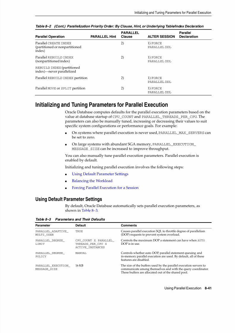
8/16/2019 Oracle Database VLDB and Partitioning Guide
http://slidepdf.com/reader/full/oracle-database-vldb-and-partitioning-guide 247/304
Initializing and Tuning Parameters for Parallel Execution
Using Parallel Execution 8-41
Initializing and Tuning Parameters for Parallel ExecutionOracle Database computes defaults for the parallel execution parameters based on the
value at database startup of CPU_COUNT and PARALLEL_THREADS_PER_CPU. Theparameters can also be manually tuned, increasing or decreasing their values to suitspecific system configurations or performance goals. For example:
■ On systems where parallel execution is never used, PARALLEL_MAX_SERVERS can be set to zero.
■ On large systems with abundant SGA memory, PARALLEL_EXECUTION_MESSAGE_SIZE can be increased to improve throughput.
You can also manually tune parallel execution parameters. Parallel execution isenabled by default.
Initializing and tuning parallel execution involves the following steps:
■ Using Default Parameter Settings■ Balancing the Workload
■ Forcing Parallel Execution for a Session
Using Default Parameter SettingsBy default, Oracle Database automatically sets parallel execution parameters, asshown in Table 8–3.
Parallel CREATE INDEX (partitioned or nonpartitionedindex)
2) 1) FORCE PARALLEL DDL
Parallel REBUILD INDEX (nonpartitioned index) 2) 1) FORCE PARALLEL DDL
REBUILD INDEX (partitionedindex)—never parallelized
Parallel REBUILD INDEX partition 2) 1) FORCE PARALLEL DDL
Parallel MOVE or SPLIT partition 2) 1) FORCE PARALLEL DDL
Table 8–3 Parameters and Their Defaults
Parameter Default Comments
PARALLEL_ADAPTIVE_MULTI_USER
TRUE Causes parallel execution SQL to throttle degree of parallelism(DOP) requests to prevent system overload.
PARALLEL_DEGREE_LIMIT
CPU_COUNT X PARALLEL_THREADS_PER_CPU XACTIVE_INSTANCES
Controls the maximum DOP a statement can have when AUTO DOP is in use.
PARALLEL_DEGREE_POLICY
MANUAL Controls whether auto DOP, parallel statement queuing andin-memory parallel execution are used. By default, all of thesefeatures are disabled.
PARALLEL_EXECUTION_MESSAGE_SIZE
16 KB The size of the buffers used by the parallel execution servers tocommunicate among themselves and with the query coordinator.These buffers are allocated out of the shared pool.
Table 8–2 (Cont.) Parallelization Priority Order: By Clause, Hint, or Underlying Table/Index Declaration
Parallel Operation PARALLEL HintPARALLELClause ALTER SESSION
ParallelDeclaration
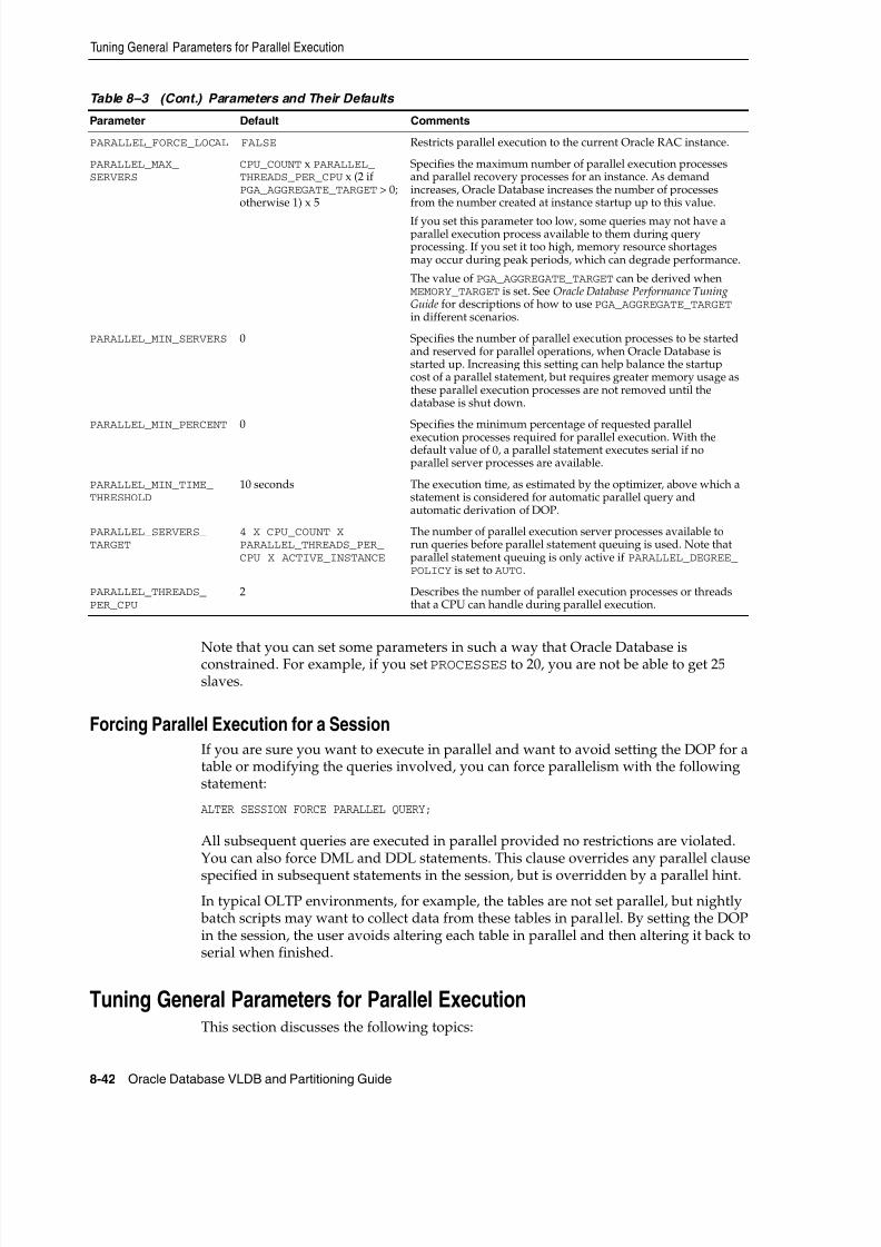
8/16/2019 Oracle Database VLDB and Partitioning Guide
http://slidepdf.com/reader/full/oracle-database-vldb-and-partitioning-guide 248/304
Tuning General Parameters for Parallel Execution
8-42 Oracle Database VLDB and Partitioning Guide
Note that you can set some parameters in such a way that Oracle Database isconstrained. For example, if you set PROCESSES to 20, you are not be able to get 25slaves.
Forcing Parallel Execution for a SessionIf you are sure you want to execute in parallel and want to avoid setting the DOP for atable or modifying the queries involved, you can force parallelism with the followingstatement:
ALTER SESSION FORCE PARALLEL QUERY;
All subsequent queries are executed in parallel provided no restrictions are violated.You can also force DML and DDL statements. This clause overrides any parallel clause
specified in subsequent statements in the session, but is overridden by a parallel hint.
In typical OLTP environments, for example, the tables are not set parallel, but nightly batch scripts may want to collect data from these tables in parallel. By setting the DOPin the session, the user avoids altering each table in parallel and then altering it back toserial when finished.
Tuning General Parameters for Parallel ExecutionThis section discusses the following topics:
PARALLEL_FORCE_LOCAL FALSE Restricts parallel execution to the current Oracle RAC instance.
PARALLEL_MAX_SERVERS
CPU_COUNT x PARALLEL_THREADS_PER_CPU x (2 ifPGA_AGGREGATE_TARGET > 0;otherwise 1) x 5
Specifies the maximum number of parallel execution processesand parallel recovery processes for an instance. As demandincreases, Oracle Database increases the number of processesfrom the number created at instance startup up to this value.
If you set this parameter too low, some queries may not have aparallel execution process available to them during queryprocessing. If you set it too high, memory resource shortagesmay occur during peak periods, which can degrade performance.
The value of PGA_AGGREGATE_TARGET can be derived whenMEMORY_TARGET is set. See Oracle Database Performance TuningGuide for descriptions of how to use PGA_AGGREGATE_TARGET in different scenarios.
PARALLEL_MIN_SERVERS 0 Specifies the number of parallel execution processes to be startedand reserved for parallel operations, when Oracle Database isstarted up. Increasing this setting can help balance the startupcost of a parallel statement, but requires greater memory usage asthese parallel execution processes are not removed until thedatabase is shut down.
PARALLEL_MIN_PERCENT 0 Specifies the minimum percentage of requested parallel
execution processes required for parallel execution. With thedefault value of 0, a parallel statement executes serial if noparallel server processes are available.
PARALLEL_MIN_TIME_THRESHOLD
10 seconds The execution time, as estimated by the optimizer, above which astatement is considered for automatic parallel query andautomatic derivation of DOP.
PARALLEL_SERVERS_TARGET
4 X CPU_COUNT XPARALLEL_THREADS_PER_CPU X ACTIVE_INSTANCE
The number of parallel execution server processes available torun queries before parallel statement queuing is used. Note thatparallel statement queuing is only active if PARALLEL_DEGREE_POLICY is set to AUTO.
PARALLEL_THREADS_PER_CPU
2 Describes the number of parallel execution processes or threadsthat a CPU can handle during parallel execution.
Table 8–3 (Cont.) Parameters and Their Defaults
Parameter Default Comments

8/16/2019 Oracle Database VLDB and Partitioning Guide
http://slidepdf.com/reader/full/oracle-database-vldb-and-partitioning-guide 249/304
Tuning General Parameters for Parallel Execution
Using Parallel Execution 8-43
■ Parameters Establishing Resource Limits for Parallel Operations
■ Parameters Affecting Resource Consumption
■ Parameters Related to I/O
Parameters Establishing Resource Limits for Parallel Operations
You can set initialization parameters to determine resource limits. The parameters thatestablish resource limits include the following:
■ PARALLEL_FORCE_LOCAL
■ PARALLEL_MAX_SERVERS
■ PARALLEL_MIN_PERCENT
■ PARALLEL_MIN_SERVERS
■ PARALLEL_MIN_TIME_THRESHOLD
■ PARALLEL_SERVERS_TARGET
■ SHARED_POOL_SIZE
PARALLEL_FORCE_LOCAL
This parameter specifies whether a SQL statement executed in parallel is restricted to asingle instance in an Oracle RAC environment. By setting this parameter to TRUE, yourestrict the scope of the parallel server processed to the single Oracle RAC instancewhere the query coordinator is running.
The recommended value for the PARALLEL_FORCE_LOCAL parameter is FALSE.
PARALLEL_MAX_SERVERS
The default value for PARALLEL_MAX_SERVERS is as follows:
(CPU_COUNT x PARALLEL_THREADS_PER_CPU x (2 if PGA_AGGREGATE_TARGET > 0; otherwise
1) x 5)
The value of PGA_AGGREGATE_TARGET can be derived when MEMORY_TARGET is set.See Oracle Database Performance Tuning Guide for descriptions of how to use PGA_AGGREGATE_TARGET in different scenarios. The above formula might not be sufficientfor parallel queries on tables with higher degree of parallelism (DOP) attributes. Werecommend users who expects to run queries of higher DOP to set PARALLEL_MAX_SERVERS as follows:
2 x DOP x NUMBER_OF_CONCURRENT_USERS
For example, setting PARALLEL_MAX_SERVERS to 64 enables you to run four parallelqueries simultaneously, if each query is using two slave sets with a DOP of eight foreach set.
When Users Have Too Many Processes When concurrent users have too many queryserver processes, memory contention (paging), I/O contention, or excessive contextswitching can occur. This contention can reduce system throughput to a level lowerthan if parallel execution were not used. Increase the PARALLEL_MAX_SERVERS valueonly if the system has sufficient memory and I/O bandwidth for the resulting load.
You can use operating system performance monitoring tools to determine how muchmemory, swap space and I/O bandwidth are free. Look at the run queue lengths for both your CPUs and disks, and the service time for I/Os on the system. Verify that the
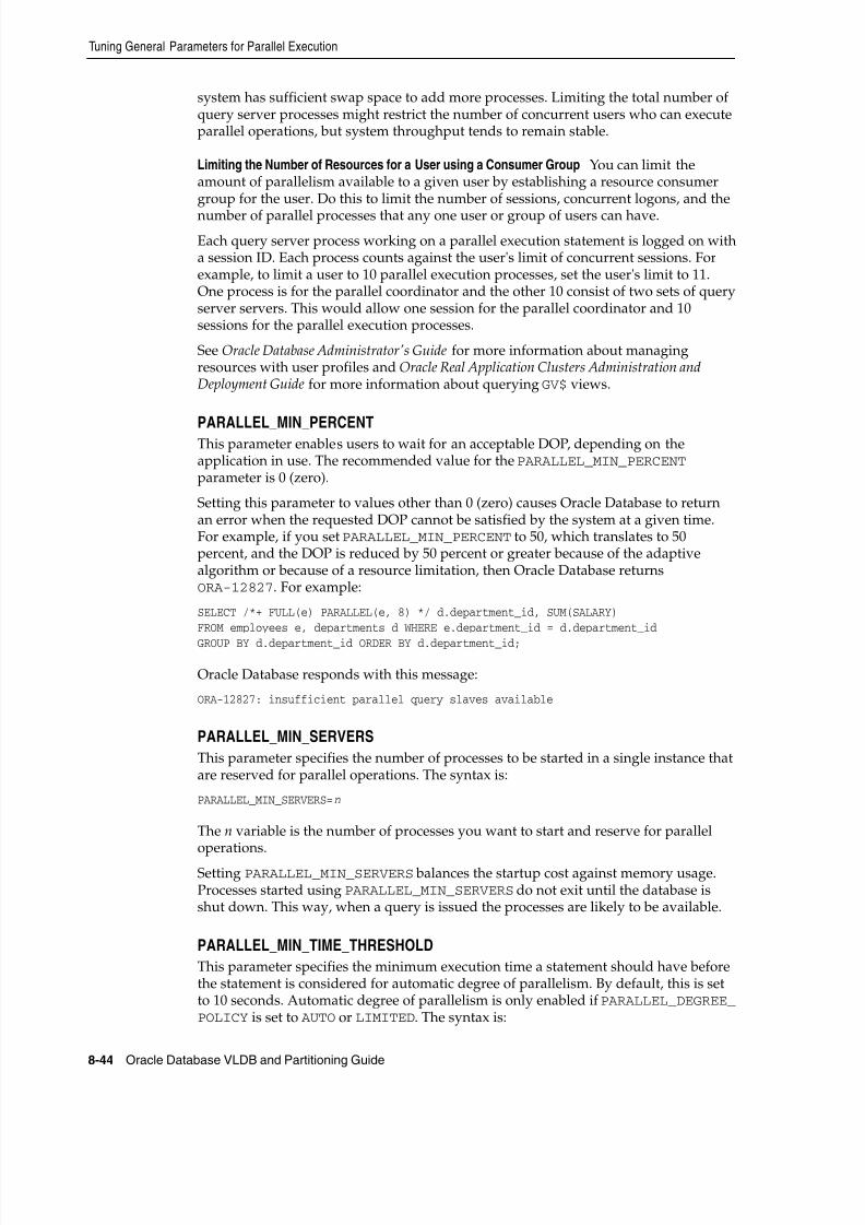
8/16/2019 Oracle Database VLDB and Partitioning Guide
http://slidepdf.com/reader/full/oracle-database-vldb-and-partitioning-guide 250/304
Tuning General Parameters for Parallel Execution
8-44 Oracle Database VLDB and Partitioning Guide
system has sufficient swap space to add more processes. Limiting the total number ofquery server processes might restrict the number of concurrent users who can executeparallel operations, but system throughput tends to remain stable.
Limiting the Number of Resources for a User using a Consumer Group You can limit theamount of parallelism available to a given user by establishing a resource consumergroup for the user. Do this to limit the number of sessions, concurrent logons, and the
number of parallel processes that any one user or group of users can have.
Each query server process working on a parallel execution statement is logged on witha session ID. Each process counts against the user's limit of concurrent sessions. Forexample, to limit a user to 10 parallel execution processes, set the user's limit to 11.One process is for the parallel coordinator and the other 10 consist of two sets of queryserver servers. This would allow one session for the parallel coordinator and 10sessions for the parallel execution processes.
See Oracle Database Administrator's Guide for more information about managingresources with user profiles and Oracle Real Application Clusters Administration andDeployment Guide for more information about querying GV$ views.
PARALLEL_MIN_PERCENTThis parameter enables users to wait for an acceptable DOP, depending on theapplication in use. The recommended value for the PARALLEL_MIN_PERCENT parameter is 0 (zero).
Setting this parameter to values other than 0 (zero) causes Oracle Database to returnan error when the requested DOP cannot be satisfied by the system at a given time.For example, if you set PARALLEL_MIN_PERCENT to 50, which translates to 50percent, and the DOP is reduced by 50 percent or greater because of the adaptivealgorithm or because of a resource limitation, then Oracle Database returnsORA-12827. For example:
SELECT /*+ FULL(e) PARALLEL(e, 8) */ d.department_id, SUM(SALARY)FROM employees e, departments d WHERE e.department_id = d.department_id
GROUP BY d.department_id ORDER BY d.department_id;
Oracle Database responds with this message:
ORA-12827: insufficient parallel query slaves available
PARALLEL_MIN_SERVERS
This parameter specifies the number of processes to be started in a single instance thatare reserved for parallel operations. The syntax is:
PARALLEL_MIN_SERVERS=n
The n variable is the number of processes you want to start and reserve for paralleloperations.
Setting PARALLEL_MIN_SERVERS balances the startup cost against memory usage.Processes started using PARALLEL_MIN_SERVERS do not exit until the database isshut down. This way, when a query is issued the processes are likely to be available.
PARALLEL_MIN_TIME_THRESHOLD
This parameter specifies the minimum execution time a statement should have beforethe statement is considered for automatic degree of parallelism. By default, this is setto 10 seconds. Automatic degree of parallelism is only enabled if PARALLEL_DEGREE_POLICY is set to AUTO or LIMITED. The syntax is:
8/16/2019 Oracle Database VLDB and Partitioning Guide
http://slidepdf.com/reader/full/oracle-database-vldb-and-partitioning-guide 251/304
Tuning General Parameters for Parallel Execution
Using Parallel Execution 8-45
PARALLEL_MIN_TIME_THRESHOLD = { AUTO | integer }
The default is AUTO.
PARALLEL_SERVERS_TARGET
This parameter specifies the number of parallel server processes allowed to runparallel statements before statement queuing is used. The recommended value forPARALLEL_SERVERS_TARGET is 4 X CPU_COUNT X PARALLEL_THREADS_PER_CPU X ACTIVE_INSTANCES.
When PARALLEL_DEGREE_POLICY is set to AUTO, statements that require parallelexecution are queued if the number of parallel processes currently in use on thesystem equals or is greater than PARALLEL_SERVERS_TARGET. This is not themaximum number of parallel server processes allowed on a system (that is controlled by PARALLEL_MAX_SERVERS). However, PARALLEL_SERVERS_TARGET and parallelstatement queuing is used to ensure and that each statement that requires parallelexecution is allocated the necessary parallel server resources and the system is notflooded with too many parallel server processes.
SHARED_POOL_SIZE
Parallel execution requires memory resources in addition to those required by serialSQL execution. Additional memory is used for communication and passing data between query server processes and the query coordinator.
Oracle Database allocates memory for query server processes from the shared pool.Tune the shared pool as follows:
■ Allow for other clients of the shared pool, such as shared cursors and storedprocedures.
■ Remember that larger values improve performance in multiuser systems, butsmaller values use less memory.
■ You can then monitor the number of buffers used by parallel execution and
compare the shared pool PX msg pool to the current high water mark reportedin output from the view V$PX_PROCESS_SYSSTAT.
By default, Oracle Database allocates parallel execution buffers from the shared pool.
If Oracle Database displays the following error on startup:
ORA-27102: out of memorySVR4 Error: 12: Not enough space
You should reduce the value for SHARED_POOL_SIZE low enough so your databasestarts. After reducing the value of SHARED_POOL_SIZE, you might see the error:
ORA-04031: unable to allocate 16084 bytes of shared memory("SHARED pool","unknown object","SHARED pool heap","PX msg pool")
If so, execute the following query to determine why Oracle Database could not allocatethe 16,084 bytes:
Note: If you do not have enough memory available, error message12853 occurs (insufficient memory for PX buffers: current stringK,max needed stringK). This is caused by having insufficient SGAmemory available for PX buffers. You must reconfigure the SGA tohave at least (MAX - CURRENT) bytes of additional memory.
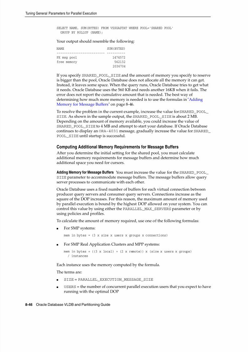
8/16/2019 Oracle Database VLDB and Partitioning Guide
http://slidepdf.com/reader/full/oracle-database-vldb-and-partitioning-guide 252/304
Tuning General Parameters for Parallel Execution
8-46 Oracle Database VLDB and Partitioning Guide
SELECT NAME, SUM(BYTES) FROM V$SGASTAT WHERE POOL='SHARED POOL'GROUP BY ROLLUP (NAME);
Your output should resemble the following:
NAME SUM(BYTES)-------------------------- ----------PX msg pool 1474572
free memory 562132 2036704
If you specify SHARED_POOL_SIZE and the amount of memory you specify to reserveis bigger than the pool, Oracle Database does not allocate all the memory it can get.Instead, it leaves some space. When the query runs, Oracle Database tries to get whatit needs. Oracle Database uses the 560 KB and needs another 16KB when it fails. Theerror does not report the cumulative amount that is needed. The best way ofdetermining how much more memory is needed is to use the formulas in "AddingMemory for Message Buffers" on page 8-46.
To resolve the problem in the current example, increase the value for SHARED_POOL_SIZE. As shown in the sample output, the SHARED_POOL_SIZE is about 2 MB.
Depending on the amount of memory available, you could increase the value ofSHARED_POOL_SIZE to 4 MB and attempt to start your database. If Oracle Databasecontinues to display an ORA-4031 message, gradually increase the value for SHARED_POOL_SIZE until startup is successful.
Computing Additional Memory Requirements for Message Buffers
After you determine the initial setting for the shared pool, you must calculateadditional memory requirements for message buffers and determine how muchadditional space you need for cursors.
Adding Memory for Message Buffers You must increase the value for the SHARED_POOL_SIZE parameter to accommodate message buffers. The message buffers allow queryserver processes to communicate with each other.
Oracle Database uses a fixed number of buffers for each virtual connection betweenproducer query servers and consumer query servers. Connections increase as thesquare of the DOP increases. For this reason, the maximum amount of memory used by parallel execution is bound by the highest DOP allowed on your system. You cancontrol this value by using either the PARALLEL_MAX_SERVERS parameter or byusing policies and profiles.
To calculate the amount of memory required, use one of the following formulas:
■ For SMP systems:
mem in bytes = (3 x size x users x groups x connections)
■ For SMP Real Application Clusters and MPP systems:
mem in bytes = ((3 x local) + (2 x remote)) x (size x users x groups)/ instances
Each instance uses the memory computed by the formula.
The terms are:
■ SIZE = PARALLEL_EXECUTION_MESSAGE_SIZE
■ USERS = the number of concurrent parallel execution users that you expect to haverunning with the optimal DOP
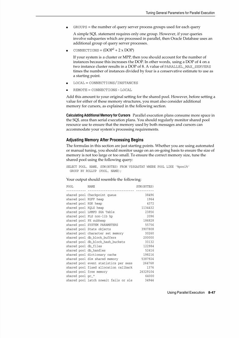
8/16/2019 Oracle Database VLDB and Partitioning Guide
http://slidepdf.com/reader/full/oracle-database-vldb-and-partitioning-guide 253/304
Tuning General Parameters for Parallel Execution
Using Parallel Execution 8-47
■ GROUPS = the number of query server process groups used for each query
A simple SQL statement requires only one group. However, if your queriesinvolve subqueries which are processed in parallel, then Oracle Database uses anadditional group of query server processes.
■ CONNECTIONS = (DOP2 + 2 x DOP)
If your system is a cluster or MPP, then you should account for the number ofinstances because this increases the DOP. In other words, using a DOP of 4 on atwo instance cluster results in a DOP of 8. A value of PARALLEL_MAX_SERVERS times the number of instances divided by four is a conservative estimate to use asa starting point.
■ LOCAL = CONNECTIONS/INSTANCES
■ REMOTE = CONNECTIONS - LOCAL
Add this amount to your original setting for the shared pool. However, before setting avalue for either of these memory structures, you must also consider additionalmemory for cursors, as explained in the following section.
Calculating Additional Memory for Cursors Parallel execution plans consume more space inthe SQL area than serial execution plans. You should regularly monitor shared poolresource use to ensure that the memory used by both messages and cursors canaccommodate your system's processing requirements.
Adjusting Memory After Processing Begins
The formulas in this section are just starting points. Whether you are using automatedor manual tuning, you should monitor usage on an on-going basis to ensure the size ofmemory is not too large or too small. To ensure the correct memory size, tune theshared pool using the following query:
SELECT POOL, NAME, SUM(BYTES) FROM V$SGASTAT WHERE POOL LIKE '%pool%' GROUP BY ROLLUP (POOL, NAME);
Your output should resemble the following:
POOL NAME SUM(BYTES)----------- -------------------------- ----------shared pool Checkpoint queue 38496shared pool KGFF heap 1964shared pool KGK heap 4372shared pool KQLS heap 1134432shared pool LRMPD SGA Table 23856shared pool PLS non-lib hp 2096shared pool PX subheap 186828shared pool SYSTEM PARAMETERS 55756shared pool State objects 3907808shared pool character set memory 30260
shared pool db_block_buffers 200000shared pool db_block_hash_buckets 33132shared pool db_files 122984shared pool db_handles 52416shared pool dictionary cache 198216shared pool dlm shared memory 5387924shared pool event statistics per sess 264768shared pool fixed allocation callback 1376shared pool free memory 26329104shared pool gc_* 64000shared pool latch nowait fails or sle 34944
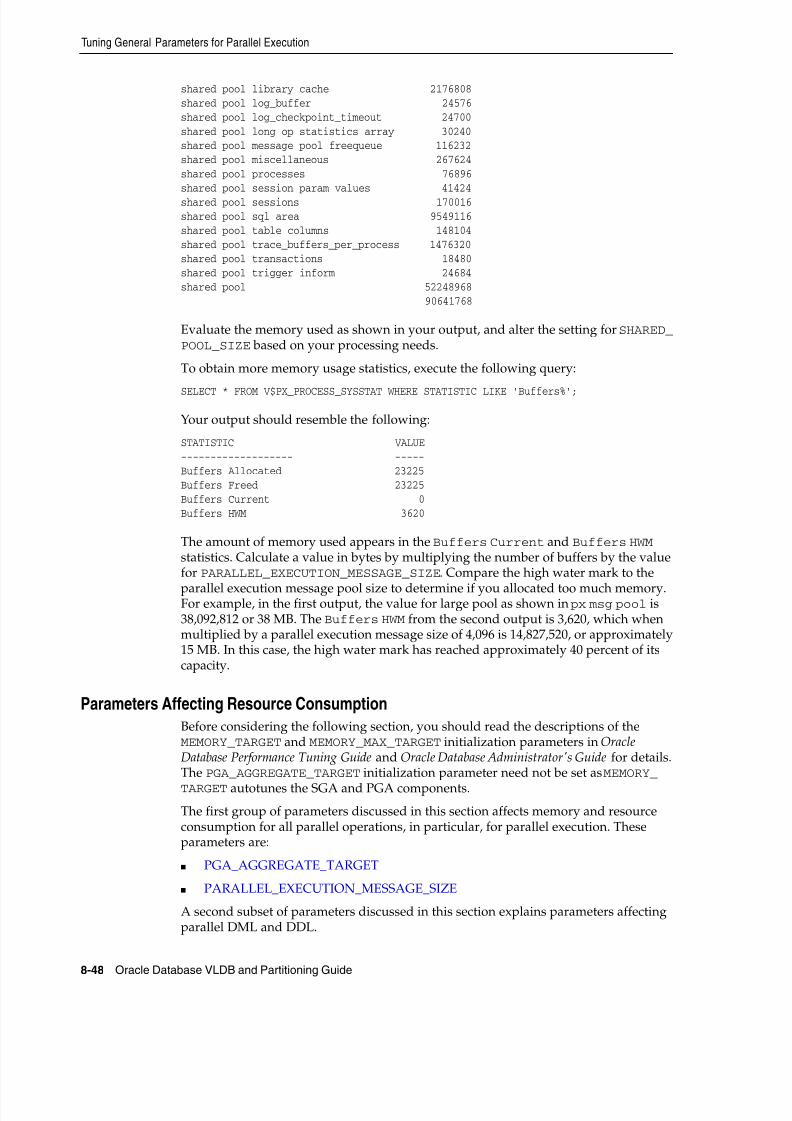
8/16/2019 Oracle Database VLDB and Partitioning Guide
http://slidepdf.com/reader/full/oracle-database-vldb-and-partitioning-guide 254/304
8/16/2019 Oracle Database VLDB and Partitioning Guide
http://slidepdf.com/reader/full/oracle-database-vldb-and-partitioning-guide 255/304
Tuning General Parameters for Parallel Execution
Using Parallel Execution 8-49
To control resource consumption, you should configure memory at two levels:
■ At the database level, so the system uses an appropriate amount of memory fromthe operating system.
■ At the operating system level for consistency. On some platforms, you might needto set operating system parameters that control the total amount of virtualmemory available, summed across all processes.
A large percentage of the memory used in data warehousing operations (compared toOLTP) is more dynamic. This memory comes from process memory (PGA), and boththe size of process memory and the number of processes can vary greatly. Use thePGA_AGGREGATE_TARGET initialization parameter to control both the processmemory and the number of processes in such cases. Explicitly setting PGA_AGGREGATE_TARGET along with MEMORY_TARGET ensures that autotuning still occurs but PGA_AGGREGATE_TARGET is not tuned below the specified value.
PGA_AGGREGATE_TARGET
You can simplify and improve the way PGA memory is allocated by enablingautomatic PGA memory management. In this mode, Oracle Database dynamicallyadjusts the size of the portion of the PGA memory dedicated to work areas, based onan overall PGA memory target explicitly set by the DBA. To enable automatic PGAmemory management, you must set the initialization parameter PGA_AGGREGATE_TARGET. For new installations, PGA_AGGREGATE_TARGET and SGA_TARGET are setautomatically by DBCA, and MEMORY_TARGET is zero. That is, automatic memorymanagement is disabled. You can enable it in Enterprise Manager on the MemoryParameters page. Therefore, automatic tuning of the aggregate PGA is enabled bydefault. However, the aggregate PGA does not grow unless you enable automaticmemory management by setting MEMORY_TARGET to a nonzero value.
See Oracle Database Performance Tuning Guide for descriptions of how to use PGA_AGGREGATE_TARGET in different scenarios.
HASH_AREA_SIZE HASH_AREA_SIZE has been deprecated and you should use PGA_
AGGREGATE_TARGET instead.
SORT_AREA_SIZE SORT_AREA_SIZE has been deprecated and you should use PGA_AGGREGATE_TARGET instead.
PARALLEL_EXECUTION_MESSAGE_SIZE
The PARALLEL_EXECUTION_MESSAGE_SIZE parameter specifies the size of the buffer used for parallel execution messages. The default value is operatingsystem-specific, but is typically 16K. This value should be adequate for mostapplications.
Parameters Affecting Resource Consumption for Parallel DML and Parallel DDL
The parameters that affect parallel DML and parallel DDL resource consumption are:
■ TRANSACTIONS
■ FAST_START_PARALLEL_ROLLBACK
■ DML_LOCKS
Parallel inserts, updates, and deletes require more resources than serial DMLoperations. Similarly, PARALLEL CREATE TABLE ... AS SELECT and PARALLEL CREATE INDEX can require more resources. For this reason, you may need to increase

8/16/2019 Oracle Database VLDB and Partitioning Guide
http://slidepdf.com/reader/full/oracle-database-vldb-and-partitioning-guide 256/304
Tuning General Parameters for Parallel Execution
8-50 Oracle Database VLDB and Partitioning Guide
the value of several additional initialization parameters. These parameters do not affect resources for queries.
TRANSACTIONS For parallel DML and DDL, each query server process starts atransaction. The parallel coordinator uses the two-phase commit protocol to committransactions; therefore, the number of transactions being processed increases by theDOP. Consequently, you might need to increase the value of the TRANSACTIONS
initialization parameter.
The TRANSACTIONS parameter specifies the maximum number of concurrenttransactions. The default assumes no parallelism. For example, if you have a DOP of20, you have 20 more new server transactions (or 40, if you have two server sets) and 1coordinator transaction. In this case, you should increase TRANSACTIONS by 21 (or 41)if the transactions are running in the same instance. If you do not set this parameter,Oracle Database sets it to a value equal to 1.1 x SESSIONS. This discussion does notapply if you are using server-managed undo.
FAST_START_PARALLEL_ROLLBACK If a system fails when there are uncommittedparallel DML or DDL transactions, you can speed up transaction recovery duringstartup by using the FAST_START_PARALLEL_ROLLBACK parameter.
This parameter controls the DOP used when recovering terminated transactions.Terminated transactions are transactions that are active before a system failure. Bydefault, the DOP is chosen to be at most two times the value of the CPU_COUNT parameter.
If the default DOP is insufficient, set the parameter to the HIGH. This gives a maximumDOP of at most four times the value of the CPU_COUNT parameter. This feature isavailable by default.
DML_LOCKS This parameter specifies the maximum number of DML locks. Its valueshould equal the total number of locks on all tables referenced by all users. A parallelDML operation's lock requirement is very different from serial DML. Parallel DMLholds many more locks, so you should increase the value of the DML_LOCKS parameter
by equal amounts.
Table 8–4 shows the types of locks acquired by coordinator and parallel executionserver processes for different types of parallel DML statements. Using thisinformation, you can determine the value required for these parameters.
Note: Parallel DML operations are not performed when the tablelock of the target table is disabled.
Table 8–4 Locks Acquired by Parallel DML Statements
Type of Statement
Coordinator Process
Acquires:
Each Parallel Execution Server
Acquires:
Parallel UPDATE or DELETE into partitioned table; WHERE clause pruned to a subset ofpartitions or subpartitions
1 table lock SX
1 partition lock X for eachpruned (sub)partition
1 table lock SX
1 partition lock NULL for eachpruned (sub)partition owned bythe query server process
1 partition-wait lock S for eachpruned (sub)partition owned bythe query server process
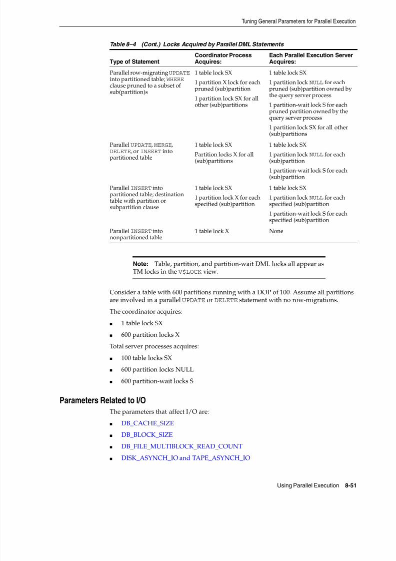
8/16/2019 Oracle Database VLDB and Partitioning Guide
http://slidepdf.com/reader/full/oracle-database-vldb-and-partitioning-guide 257/304
Tuning General Parameters for Parallel Execution
Using Parallel Execution 8-51
Consider a table with 600 partitions running with a DOP of 100. Assume all partitionsare involved in a parallel UPDATE or DELETE statement with no row-migrations.
The coordinator acquires:
■ 1 table lock SX
■ 600 partition locks X
Total server processes acquires:
■ 100 table locks SX
■ 600 partition locks NULL
■ 600 partition-wait locks S
Parameters Related to I/OThe parameters that affect I/O are:
■ DB_CACHE_SIZE
■ DB_BLOCK_SIZE
■ DB_FILE_MULTIBLOCK_READ_COUNT
■ DISK_ASYNCH_IO and TAPE_ASYNCH_IO
Parallel row-migrating UPDATE into partitioned table; WHERE clause pruned to a subset ofsub(partition)s
1 table lock SX
1 partition X lock for eachpruned (sub)partition
1 partition lock SX for allother (sub)partitions
1 table lock SX
1 partition lock NULL for eachpruned (sub)partition owned by
the query server process1 partition-wait lock S for eachpruned partition owned by thequery server process
1 partition lock SX for all other(sub)partitions
Parallel UPDATE, MERGE,DELETE, or INSERT intopartitioned table
1 table lock SX
Partition locks X for all(sub)partitions
1 table lock SX
1 partition lock NULL for each(sub)partition
1 partition-wait lock S for each(sub)partition
Parallel INSERT into
partitioned table; destinationtable with partition orsubpartition clause
1 table lock SX
1 partition lock X for eachspecified (sub)partition
1 table lock SX
1 partition lock NULL for eachspecified (sub)partition
1 partition-wait lock S for eachspecified (sub)partition
Parallel INSERT intononpartitioned table
1 table lock X None
Note: Table, partition, and partition-wait DML locks all appear asTM locks in the V$LOCK view.
Table 8–4 (Cont.) Locks Acquired by Parallel DML Statements
Type of StatementCoordinator ProcessAcquires:
Each Parallel Execution ServerAcquires:
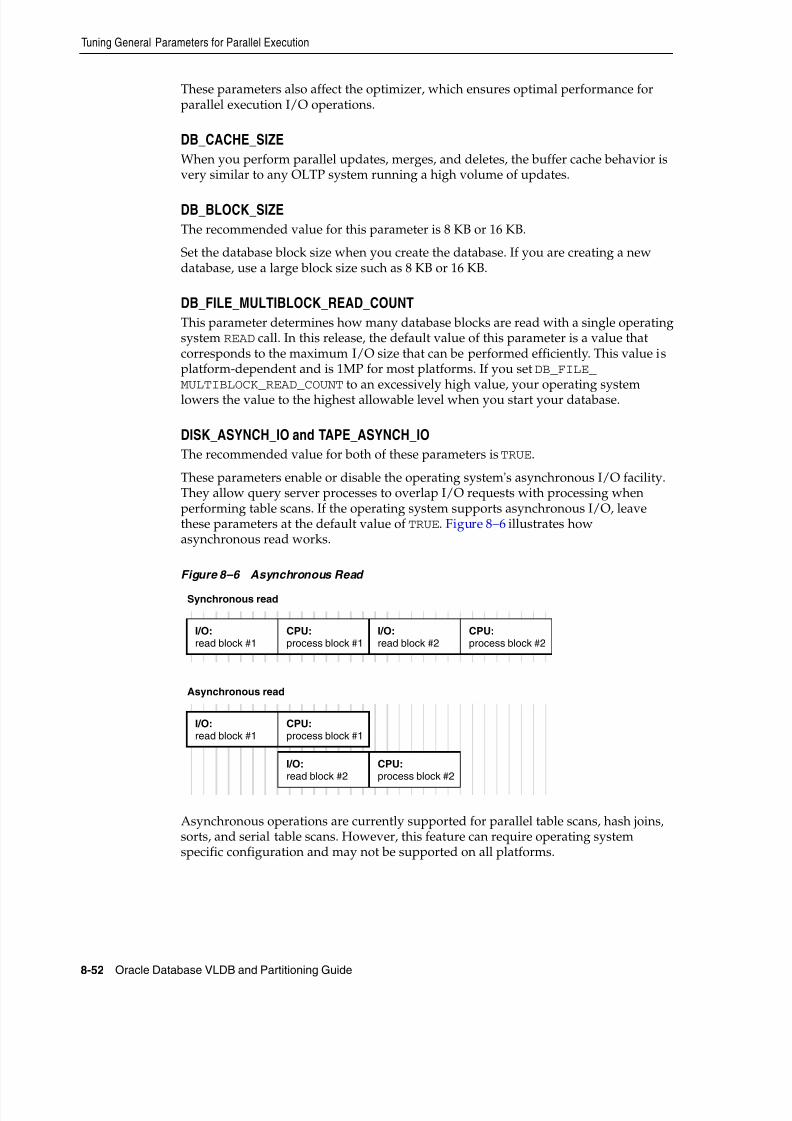
8/16/2019 Oracle Database VLDB and Partitioning Guide
http://slidepdf.com/reader/full/oracle-database-vldb-and-partitioning-guide 258/304
Tuning General Parameters for Parallel Execution
8-52 Oracle Database VLDB and Partitioning Guide
These parameters also affect the optimizer, which ensures optimal performance forparallel execution I/O operations.
DB_CACHE_SIZE
When you perform parallel updates, merges, and deletes, the buffer cache behavior isvery similar to any OLTP system running a high volume of updates.
DB_BLOCK_SIZE
The recommended value for this parameter is 8 KB or 16 KB.
Set the database block size when you create the database. If you are creating a newdatabase, use a large block size such as 8 KB or 16 KB.
DB_FILE_MULTIBLOCK_READ_COUNT
This parameter determines how many database blocks are read with a single operatingsystem READ call. In this release, the default value of this parameter is a value thatcorresponds to the maximum I/O size that can be performed efficiently. This value isplatform-dependent and is 1MP for most platforms. If you set DB_FILE_MULTIBLOCK_READ_COUNT to an excessively high value, your operating systemlowers the value to the highest allowable level when you start your database.
DISK_ASYNCH_IO and TAPE_ASYNCH_IO
The recommended value for both of these parameters is TRUE.
These parameters enable or disable the operating system's asynchronous I/O facility.They allow query server processes to overlap I/O requests with processing whenperforming table scans. If the operating system supports asynchronous I/O, leavethese parameters at the default value of TRUE. Figure 8–6 illustrates howasynchronous read works.
Figure 8–6 Asynchronous Read
Asynchronous operations are currently supported for parallel table scans, hash joins,sorts, and serial table scans. However, this feature can require operating systemspecific configuration and may not be supported on all platforms.
I/O:read block #1
CPU:process block #1
I/O:read block #2
CPU:process block #2
Synchronous read
I/O:read block #1
CPU:process block #1
I/O:read block #2
CPU:process block #2
Asynchronous read
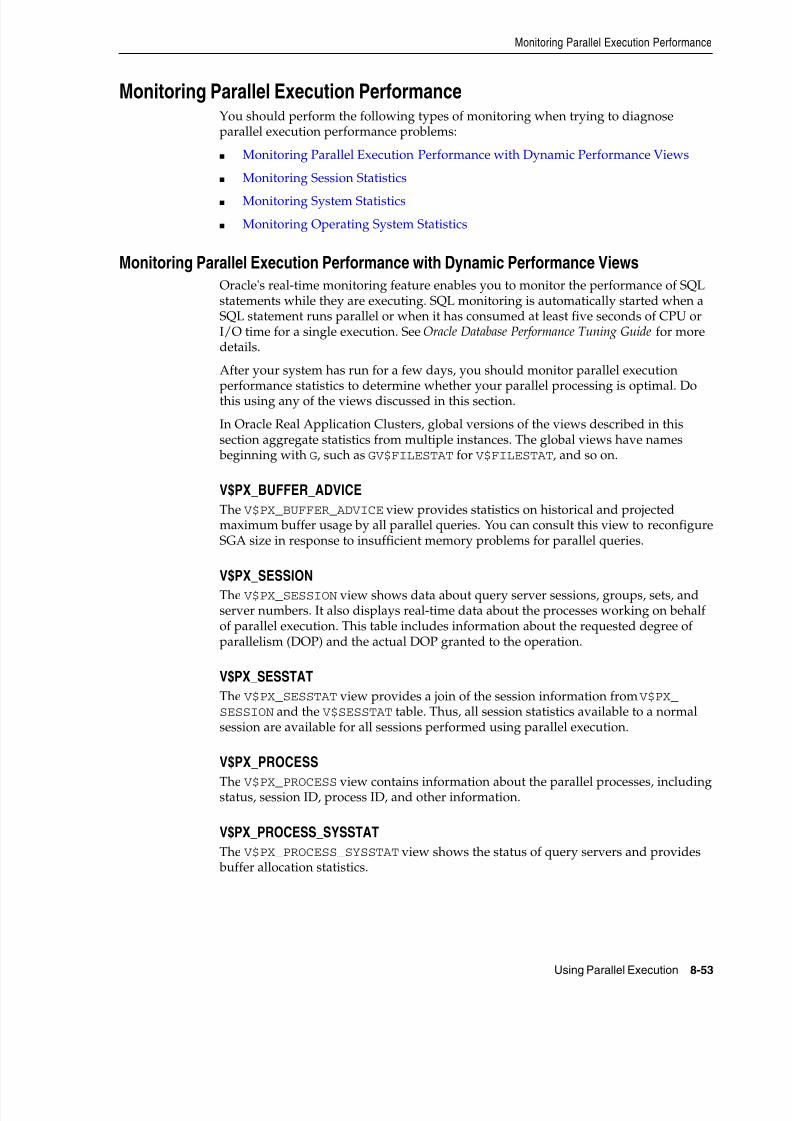
8/16/2019 Oracle Database VLDB and Partitioning Guide
http://slidepdf.com/reader/full/oracle-database-vldb-and-partitioning-guide 259/304
Monitoring Parallel Execution Performance
Using Parallel Execution 8-53
Monitoring Parallel Execution PerformanceYou should perform the following types of monitoring when trying to diagnoseparallel execution performance problems:
■ Monitoring Parallel Execution Performance with Dynamic Performance Views
■ Monitoring Session Statistics
■ Monitoring System Statistics
■ Monitoring Operating System Statistics
Monitoring Parallel Execution Performance with Dynamic Performance ViewsOracle's real-time monitoring feature enables you to monitor the performance of SQLstatements while they are executing. SQL monitoring is automatically started when aSQL statement runs parallel or when it has consumed at least five seconds of CPU orI/O time for a single execution. See Oracle Database Performance Tuning Guide for moredetails.
After your system has run for a few days, you should monitor parallel execution
performance statistics to determine whether your parallel processing is optimal. Dothis using any of the views discussed in this section.
In Oracle Real Application Clusters, global versions of the views described in thissection aggregate statistics from multiple instances. The global views have names beginning with G, such as GV$FILESTAT for V$FILESTAT, and so on.
V$PX_BUFFER_ADVICE
The V$PX_BUFFER_ADVICE view provides statistics on historical and projectedmaximum buffer usage by all parallel queries. You can consult this view to reconfigureSGA size in response to insufficient memory problems for parallel queries.
V$PX_SESSION
The V$PX_SESSION view shows data about query server sessions, groups, sets, andserver numbers. It also displays real-time data about the processes working on behalfof parallel execution. This table includes information about the requested degree ofparallelism (DOP) and the actual DOP granted to the operation.
V$PX_SESSTAT
The V$PX_SESSTAT view provides a join of the session information from V$PX_SESSION and the V$SESSTAT table. Thus, all session statistics available to a normalsession are available for all sessions performed using parallel execution.
V$PX_PROCESS
The V$PX_PROCESS view contains information about the parallel processes, includingstatus, session ID, process ID, and other information.
V$PX_PROCESS_SYSSTAT
The V$PX_PROCESS_SYSSTAT view shows the status of query servers and provides buffer allocation statistics.

8/16/2019 Oracle Database VLDB and Partitioning Guide
http://slidepdf.com/reader/full/oracle-database-vldb-and-partitioning-guide 260/304
Monitoring Parallel Execution Performance
8-54 Oracle Database VLDB and Partitioning Guide
V$PQ_SESSTAT
The V$PQ_SESSTAT view shows the status of all current server groups in the systemsuch as data about how queries allocate processes and how the multiuser and load balancing algorithms are affecting the default and hinted values.
You might need to adjust some parameter settings to improve performance afterreviewing data from these views. In this case, refer to the discussion of "Tuning
General Parameters for Parallel Execution" on page 8-42. Query these viewsperiodically to monitor the progress of long-running parallel operations.
For many dynamic performance views, you must set the parameter TIMED_STATISTICS to TRUE in order for Oracle Database to collect statistics for each view.You can use the ALTER SYSTEM or ALTER SESSION statements to turn TIMED_STATISTICS on and off.
V$PQ_TQSTAT
As a simple example, consider a hash join between two tables, with a join on a columnwith only two distinct values. At best, this hash function has one hash value to parallelexecution server A and the other to parallel execution server B. A DOP of two is fine, but, if it is four, then at least two parallel execution servers have no work. To discover
this type of skew, use a query similar to the following example:
SELECT dfo_number, tq_id, server_type, process, num_rowsFROM V$PQ_TQSTAT ORDER BY dfo_number DESC, tq_id, server_type, process;
The best way to resolve this problem might be to choose a different join method; anested loop join might be the best option. Alternatively, if one join table is smallrelative to the other, a BROADCAST distribution method can be hinted using PQ_DISTRIBUTE hint. Note that the optimizer considers the BROADCAST distributionmethod, but requires OPTIMIZER_FEATURES_ENABLE set to 9.0.2 or higher.
Now, assume that you have a join key with high cardinality, but one value containsmost of the data, for example, lava lamp sales by year. The only year that had big saleswas 1968, and the parallel execution server for the 1968 records is overwhelmed. You
should use the same corrective actions as described previously.
The V$PQ_TQSTAT view provides a detailed report of message traffic at the tablequeue level. V$PQ_TQSTAT data is valid only when queried from a session that isexecuting parallel SQL statements. A table queue is the pipeline between query servergroups, between the parallel coordinator and a query server group, or between aquery server group and the coordinator. The table queues are represented explicitly inthe operation column by PX SEND <partitioning type> (for example, PX SENDHASH) and PX RECEIVE. For backward compatibility, the row labels of PARALLEL_TO_PARALLEL, SERIAL_TO_PARALLEL, or PARALLEL_TO_SERIAL continue to havethe same semantics as previous releases and can be used as before to deduce the tablequeue allocation. In addition, the top of the parallel plan is marked by a new nodewith operation PX COORDINATOR.
V$PQ_TQSTAT has a row for each query server process that reads from or writes to ineach table queue. A table queue connecting 10 consumer processes to 10 producerprocesses has 20 rows in the view. Sum the bytes column and group by TQ_ID, thetable queue identifier, to obtain the total number of bytes sent through each tablequeue. Compare this with the optimizer estimates; large variations might indicate aneed to analyze the data using a larger sample.
Compute the variance of bytes grouped by TQ_ID. Large variances indicate workloadimbalances. You should investigate large variances to determine whether theproducers start out with unequal distributions of data, or whether the distribution
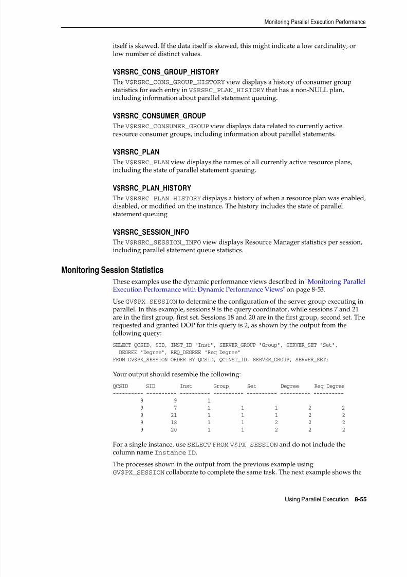
8/16/2019 Oracle Database VLDB and Partitioning Guide
http://slidepdf.com/reader/full/oracle-database-vldb-and-partitioning-guide 261/304
Monitoring Parallel Execution Performance
Using Parallel Execution 8-55
itself is skewed. If the data itself is skewed, this might indicate a low cardinality, orlow number of distinct values.
V$RSRC_CONS_GROUP_HISTORY
The V$RSRC_CONS_GROUP_HISTORY view displays a history of consumer groupstatistics for each entry in V$RSRC_PLAN_HISTORY that has a non-NULL plan,
including information about parallel statement queuing.
V$RSRC_CONSUMER_GROUP
The V$RSRC_CONSUMER_GROUP view displays data related to currently activeresource consumer groups, including information about parallel statements.
V$RSRC_PLAN
The V$RSRC_PLAN view displays the names of all currently active resource plans,including the state of parallel statement queuing.
V$RSRC_PLAN_HISTORY
The V$RSRC_PLAN_HISTORY displays a history of when a resource plan was enabled,disabled, or modified on the instance. The history includes the state of parallelstatement queuing
V$RSRC_SESSION_INFO
The V$RSRC_SESSION_INFO view displays Resource Manager statistics per session,including parallel statement queue statistics.
Monitoring Session StatisticsThese examples use the dynamic performance views described in "Monitoring ParallelExecution Performance with Dynamic Performance Views" on page 8-53.
Use GV$PX_SESSION to determine the configuration of the server group executing inparallel. In this example, sessions 9 is the query coordinator, while sessions 7 and 21are in the first group, first set. Sessions 18 and 20 are in the first group, second set. Therequested and granted DOP for this query is 2, as shown by the output from thefollowing query:
SELECT QCSID, SID, INST_ID "Inst", SERVER_GROUP "Group", SERVER_SET "Set", DEGREE "Degree", REQ_DEGREE "Req Degree"FROM GV$PX_SESSION ORDER BY QCSID, QCINST_ID, SERVER_GROUP, SERVER_SET;
Your output should resemble the following:
QCSID SID Inst Group Set Degree Req Degree---------- ---------- ---------- ---------- ---------- ---------- ----------
9 9 19 7 1 1 1 2 29 21 1 1 1 2 29 18 1 1 2 2 29 20 1 1 2 2 2
For a single instance, use SELECT FROM V$PX_SESSION and do not include thecolumn name Instance ID.
The processes shown in the output from the previous example usingGV$PX_SESSION collaborate to complete the same task. The next example shows the
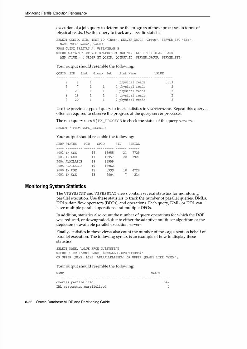
8/16/2019 Oracle Database VLDB and Partitioning Guide
http://slidepdf.com/reader/full/oracle-database-vldb-and-partitioning-guide 262/304
Monitoring Parallel Execution Performance
8-56 Oracle Database VLDB and Partitioning Guide
execution of a join query to determine the progress of these processes in terms ofphysical reads. Use this query to track any specific statistic:
SELECT QCSID, SID, INST_ID "Inst", SERVER_GROUP "Group", SERVER_SET "Set", NAME "Stat Name", VALUEFROM GV$PX_SESSTAT A, V$STATNAME B
WHERE A.STATISTIC# = B.STATISTIC# AND NAME LIKE 'PHYSICAL READS' AND VALUE > 0 ORDER BY QCSID, QCINST_ID, SERVER_GROUP, SERVER_SET;
Your output should resemble the following:
QCSID SID Inst Group Set Stat Name VALUE------ ----- ------ ------ ------ ------------------ ----------
9 9 1 physical reads 38639 7 1 1 1 physical reads 29 21 1 1 1 physical reads 29 18 1 1 2 physical reads 29 20 1 1 2 physical reads 2
Use the previous type of query to track statistics in V$STATNAME. Repeat this query asoften as required to observe the progress of the query server processes.
The next query uses V$PX_PROCESS to check the status of the query servers.SELECT * FROM V$PX_PROCESS;
Your output should resemble the following:
SERV STATUS PID SPID SID SERIAL---- --------- ------ --------- ------ ------P002 IN USE 16 16955 21 7729P003 IN USE 17 16957 20 2921P004 AVAILABLE 18 16959P005 AVAILABLE 19 16962P000 IN USE 12 6999 18 4720P001 IN USE 13 7004 7 234
Monitoring System StatisticsThe V$SYSSTAT and V$SESSTAT views contain several statistics for monitoringparallel execution. Use these statistics to track the number of parallel queries, DMLs,DDLs, data flow operators (DFOs), and operations. Each query, DML, or DDL canhave multiple parallel operations and multiple DFOs.
In addition, statistics also count the number of query operations for which the DOPwas reduced, or downgraded, due to either the adaptive multiuser algorithm or thedepletion of available parallel execution servers.
Finally, statistics in these views also count the number of messages sent on behalf ofparallel execution. The following syntax is an example of how to display thesestatistics:
SELECT NAME, VALUE FROM GV$SYSSTAT WHERE UPPER (NAME) LIKE '%PARALLEL OPERATIONS%'OR UPPER (NAME) LIKE '%PARALLELIZED%' OR UPPER (NAME) LIKE '%PX%';
Your output should resemble the following:
NAME VALUE-------------------------------------------------- ----------queries parallelized 347DML statements parallelized 0
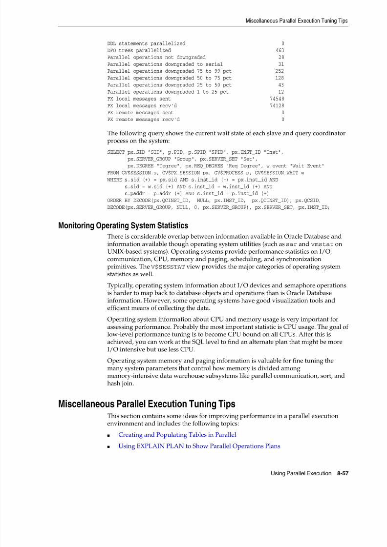
8/16/2019 Oracle Database VLDB and Partitioning Guide
http://slidepdf.com/reader/full/oracle-database-vldb-and-partitioning-guide 263/304
Miscellaneous Parallel Execution Tuning Tips
Using Parallel Execution 8-57
DDL statements parallelized 0DFO trees parallelized 463Parallel operations not downgraded 28Parallel operations downgraded to serial 31Parallel operations downgraded 75 to 99 pct 252Parallel operations downgraded 50 to 75 pct 128Parallel operations downgraded 25 to 50 pct 43Parallel operations downgraded 1 to 25 pct 12PX local messages sent 74548PX local messages recv'd 74128PX remote messages sent 0PX remote messages recv'd 0
The following query shows the current wait state of each slave and query coordinatorprocess on the system:
SELECT px.SID "SID", p.PID, p.SPID "SPID", px.INST_ID "Inst", px.SERVER_GROUP "Group", px.SERVER_SET "Set", px.DEGREE "Degree", px.REQ_DEGREE "Req Degree", w.event "Wait Event"FROM GV$SESSION s, GV$PX_SESSION px, GV$PROCESS p, GV$SESSION_WAIT w
WHERE s.sid (+) = px.sid AND s.inst_id (+) = px.inst_id AND s.sid = w.sid (+) AND s.inst_id = w.inst_id (+) AND
s.paddr = p.addr (+) AND s.inst_id = p.inst_id (+)ORDER BY DECODE(px.QCINST_ID, NULL, px.INST_ID, px.QCINST_ID), px.QCSID,DECODE(px.SERVER_GROUP, NULL, 0, px.SERVER_GROUP), px.SERVER_SET, px.INST_ID;
Monitoring Operating System StatisticsThere is considerable overlap between information available in Oracle Database andinformation available though operating system utilities (such as sar and vmstat onUNIX-based systems). Operating systems provide performance statistics on I/O,communication, CPU, memory and paging, scheduling, and synchronizationprimitives. The V$SESSTAT view provides the major categories of operating systemstatistics as well.
Typically, operating system information about I/O devices and semaphore operationsis harder to map back to database objects and operations than is Oracle Databaseinformation. However, some operating systems have good visualization tools andefficient means of collecting the data.
Operating system information about CPU and memory usage is very important forassessing performance. Probably the most important statistic is CPU usage. The goal oflow-level performance tuning is to become CPU bound on all CPUs. After this isachieved, you can work at the SQL level to find an alternate plan that might be moreI/O intensive but use less CPU.
Operating system memory and paging information is valuable for fine tuning themany system parameters that control how memory is divided amongmemory-intensive data warehouse subsystems like parallel communication, sort, and
hash join.
Miscellaneous Parallel Execution Tuning TipsThis section contains some ideas for improving performance in a parallel executionenvironment and includes the following topics:
■ Creating and Populating Tables in Parallel
■ Using EXPLAIN PLAN to Show Parallel Operations Plans

8/16/2019 Oracle Database VLDB and Partitioning Guide
http://slidepdf.com/reader/full/oracle-database-vldb-and-partitioning-guide 264/304
Miscellaneous Parallel Execution Tuning Tips
8-58 Oracle Database VLDB and Partitioning Guide
■ Additional Considerations for Parallel DML
■ Creating Indexes in Parallel
■ Parallel DML Tips
■ Incremental Data Loading in Parallel
Creating and Populating Tables in ParallelOracle Database cannot return results to a user process in parallel. If a query returns alarge number of rows, execution of the query might indeed be faster. However, theuser process can only receive the rows serially. To optimize parallel executionperformance for queries that retrieve large result sets, use PARALLEL CREATE TABLE ... AS SELECT or direct-path INSERT to store the result set in the database. At a latertime, users can view the result set serially.
Performing the SELECT in parallel does not influence the CREATE statement. If theCREATE is parallel, however, the optimizer tries to make the SELECT run in parallelalso.
When combined with the NOLOGGING option, the parallel version of CREATE TABLE ...
AS SELECT provides a very efficient intermediate table facility, for example:CREATE TABLE summary PARALLEL NOLOGGING AS SELECT dim_1, dim_2 ...,SUM (meas_1)FROM facts GROUP BY dim_1, dim_2;
These tables can also be incrementally loaded with parallel INSERT. You can takeadvantage of intermediate tables using the following techniques:
■ Common subqueries can be computed once and referenced many times. This canallow some queries against star schemas (in particular, queries without selective WHERE-clause predicates) to be better parallelized. Note that star queries with
selective WHERE-clause predicates using the star-transformation technique can beeffectively parallelized automatically without any modification to the SQL.
■ Decompose complex queries into simpler steps to provide application-levelcheckpoint or restart. For example, a complex multitable join on a one terabytedatabase could run for dozens of hours. A failure during this query would meanstarting over from the beginning. Using CREATE TABLE ... AS SELECT orPARALLEL INSERT AS SELECT, you can rewrite the query as a sequence ofsimpler queries that run for a few hours each. If a system failure occurs, the querycan be restarted from the last completed step.
■ Implement manual parallel deletes efficiently by creating a new table that omitsthe unwanted rows from the original table, and then dropping the original table.Alternatively, you can use the convenient parallel delete feature, which directlydeletes rows from the original table.
■ Create summary tables for efficient multidimensional drill-down analysis. Forexample, a summary table might store the sum of revenue grouped by month, brand, region, and salesman.
■ Reorganize tables, eliminating chained rows, compressing free space, and so on, by copying the old table to a new table. This is much faster than export/importand easier than reloading.
Be sure to use the DBMS_STATS package to gather optimizer statistics on newlycreated tables. To avoid I/O bottlenecks, specify a tablespace that is striped across atleast as many physical disks as CPUs. To avoid fragmentation in allocating space, the
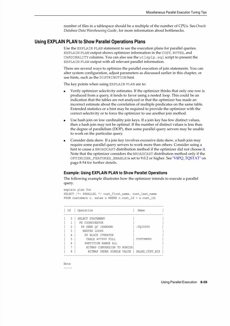
8/16/2019 Oracle Database VLDB and Partitioning Guide
http://slidepdf.com/reader/full/oracle-database-vldb-and-partitioning-guide 265/304
Miscellaneous Parallel Execution Tuning Tips
Using Parallel Execution 8-59
number of files in a tablespace should be a multiple of the number of CPUs. See OracleDatabase Data Warehousing Guide, for more information about bottlenecks.
Using EXPLAIN PLAN to Show Parallel Operations PlansUse the EXPLAIN PLAN statement to see the execution plans for parallel queries.EXPLAIN PLAN output shows optimizer information in the COST, BYTES, and
CARDINALITY columns. You can also use the utlxplp.sql script to present theEXPLAIN PLAN output with all relevant parallel information.
There are several ways to optimize the parallel execution of join statements. You canalter system configuration, adjust parameters as discussed earlier in this chapter, oruse hints, such as the DISTRIBUTION hint.
The key points when using EXPLAIN PLAN are to:
■ Verify optimizer selectivity estimates. If the optimizer thinks that only one row isproduced from a query, it tends to favor using a nested loop. This could be anindication that the tables are not analyzed or that the optimizer has made anincorrect estimate about the correlation of multiple predicates on the same table.Extended statistics or a hint may be required to provide the optimizer with the
correct selectivity or to force the optimizer to use another join method.■ Use hash join on low cardinality join keys. If a join key has few distinct values,
then a hash join may not be optimal. If the number of distinct values is less thanthe degree of parallelism (DOP), then some parallel query servers may be unableto work on the particular query.
■ Consider data skew. If a join key involves excessive data skew, a hash join mayrequire some parallel query servers to work more than others. Consider using ahint to cause a BROADCAST distribution method if the optimizer did not choose it.Note that the optimizer considers the BROADCAST distribution method only if theOPTIMIZER_FEATURES_ENABLE is set to 9.0.2 or higher. See "V$PQ_TQSTAT" onpage 8-54 for further details.
Example: Using EXPLAIN PLAN to Show Parallel OperationsThe following example illustrates how the optimizer intends to execute a parallelquery.
explain plan forSELECT /*+ PARALLEL */ cust_first_name, cust_last_nameFROM customers c, sales s WHERE c.cust_id = s.cust_id;
----------------------------------------------------------| Id | Operation | Name |----------------------------------------------------------| 0 | SELECT STATEMENT | || 1 | PX COORDINATOR | |
| 2 | PX SEND QC (RANDOM) | :TQ10000 || 3 | NESTED LOOPS | || 4 | PX BLOCK ITERATOR | || 5 | TABLE ACCESS FULL | CUSTOMERS || 6 | PARTITION RANGE ALL | || 7 | BITMAP CONVERSION TO ROWIDS| || 8 | BITMAP INDEX SINGLE VALUE | SALES_CUST_BIX |----------------------------------------------------------
Note-----
8/16/2019 Oracle Database VLDB and Partitioning Guide
http://slidepdf.com/reader/full/oracle-database-vldb-and-partitioning-guide 266/304
Miscellaneous Parallel Execution Tuning Tips
8-60 Oracle Database VLDB and Partitioning Guide
- Computed Degree of Parallelism is 2 - Degree of Parallelism of 2 is derived from scan of object SH.CUSTOMERS
Additional Considerations for Parallel DMLWhen you want to refresh your data warehouse database using parallel insert, update,or delete on a data warehouse, there are additional issues to consider when designing
the physical database. These considerations do not affect parallel execution operations.These issues are:
■ Parallel DML and Direct-Path Restrictions
■ Limitation on the Degree of Parallelism
■ Increasing INITRANS
■ Limitation on Available Number of Transaction Free Lists for Segments
■ Using Multiple Archivers
■ Database Writer Process (DBWn) Workload
■ [NO]LOGGING Clause
Parallel DML and Direct-Path Restrictions
If a parallel restriction is violated, the operation is simply performed serially. If adirect-path INSERT restriction is violated, then the APPEND hint is ignored and aconventional insert is performed. No error message is returned.
Limitation on the Degree of Parallelism
For tables that do not have the parallel DML itl invariant property (tables created before Oracle Database release 9.2 or tables that were created with the COMPATIBLE initialization parameter set to less than 9.2), the degree of parallelism (DOP) equalsthe number of partitions or subpartitions. That means that, if the table is notpartitioned, the query runs in serial. To see what tables do not have this property, issue
the following statement:
SELECT u.name, o.name FROM obj$ o, tab$ t, user$ u WHERE o.obj# = t.obj# AND o.owner# = u.user# AND bitand(t.property,536870912) != 536870912;
For information about the interested transaction list (ITL), also called the transactiontable, refer to Oracle Database Concepts.
Increasing INITRANS
If you have global indexes, a global index segment and global index blocks are shared by server processes of the same parallel DML statement. Even if the operations are notperformed against the same row, the server processes can share the same index blocks.
Each server transaction needs one transaction entry in the index block header before itcan make changes to a block. Therefore, in the CREATE INDEX or ALTER INDEX statements, you should set INITRANS, the initial number of transactions allocatedwithin each data block, to a large value, such as the maximum DOP against this index.
Limitation on Available Number of Transaction Free Lists for Segments
There is a limitation on the available number of transaction free lists for segments indictionary-managed tablespaces. After a segment has been created, the number ofprocess and transaction free lists is fixed and cannot be altered. If you specify a largenumber of process free lists in the segment header, you might find that this limits the
8/16/2019 Oracle Database VLDB and Partitioning Guide
http://slidepdf.com/reader/full/oracle-database-vldb-and-partitioning-guide 267/304
Miscellaneous Parallel Execution Tuning Tips
Using Parallel Execution 8-61
number of transaction free lists that are available. You can abate this limitation the nexttime you re-create the segment header by decreasing the number of process free lists;this leaves more room for transaction free lists in the segment header.
For UPDATE and DELETE operations, each server process can require its owntransaction free list. The parallel DML DOP is thus effectively limited by the smallestnumber of transaction free lists available on the table and on any of the global indexes
the DML statement must maintain. For example, if the table has 25 transaction freelists and the table has two global indexes, one with 50 transaction free lists and onewith 30 transaction free lists, the DOP is limited to 25. If the table had 40 transactionfree lists, the DOP would have been limited to 30.
The FREELISTS parameter of the STORAGE clause is used to set the number of processfree lists. By default, no process free lists are created.
The default number of transaction free lists depends on the block size. For example, ifthe number of process free lists is not set explicitly, a 4 KB block has about 80transaction free lists by default. The minimum number of transaction free lists is 25.
Using Multiple Archivers
Parallel DDL and parallel DML operations can generate a large amount of redo logs. Asingle ARCH process to archive these redo logs might not be able to keep up. To avoidthis problem, you can spawn multiple archiver processes. This can be done manuallyor by using a job queue.
Database Writer Process (DBWn) Workload
Parallel DML operations dirty a large number of data, index, and undo blocks in the buffer cache during a short interval. For example, suppose you see a high number offree_buffer_waits after querying the V$SYSTEM_EVENT view, as in the followingsyntax:
SELECT TOTAL_WAITS FROM V$SYSTEM_EVENT WHERE EVENT = 'FREE BUFFER WAITS';
In this case, you should consider increasing the DBWn
processes. If there are no waitsfor free buffers, the query does not return any rows.
[NO]LOGGING Clause
The [NO]LOGGING clause applies to tables, partitions, tablespaces, and indexes.Virtually no log is generated for certain operations (such as direct-path INSERT) if theNOLOGGING clause is used. The NOLOGGING attribute is not specified at the INSERT statement level but is instead specified when using the ALTER or CREATE statementfor a table, partition, index, or tablespace.
When a table or index has NOLOGGING set, neither parallel nor serial direct-pathINSERT operations generate redo logs. Processes running with the NOLOGGING optionset run faster because no redo is generated. However, after a NOLOGGING operation
against a table, partition, or index, if a media failure occurs before a backup is taken,then all tables, partitions, and indexes that have been modified might be corrupted.
Direct-path INSERT operations (except for dictionary updates) never generate redologs if the NOLOGGING clause is used. The NOLOGGING attribute does not affect undo,only redo. To be precise, NOLOGGING allows the direct-path INSERT operation togenerate a negligible amount of redo (range-invalidation redo, as opposed to fullimage redo).
8/16/2019 Oracle Database VLDB and Partitioning Guide
http://slidepdf.com/reader/full/oracle-database-vldb-and-partitioning-guide 268/304
Miscellaneous Parallel Execution Tuning Tips
8-62 Oracle Database VLDB and Partitioning Guide
For backward compatibility, [UN]RECOVERABLE is still supported as an alternatekeyword with the CREATE TABLE statement. This alternate keyword might not besupported, however, in future releases.
At the tablespace level, the logging clause specifies the default logging attribute for alltables, indexes, and partitions created in the tablespace. When an existing tablespacelogging attribute is changed by the ALTER TABLESPACE statement, then all tables,
indexes, and partitions created after the ALTER statement have the new loggingattribute; existing ones do not change their logging attributes. The tablespace-levellogging attribute can be overridden by the specifications at the table, index, orpartition level.
The default logging attribute is LOGGING. However, if you have put the database inNOARCHIVELOG mode, by issuing ALTER DATABASE NOARCHIVELOG, then alloperations that can be done without logging do not generate logs, regardless of thespecified logging attribute.
Creating Indexes in ParallelMultiple processes can work simultaneously to create an index. By dividing the worknecessary to create an index among multiple server processes, Oracle Database can
create the index more quickly than if a single server process created the indexsequentially.
Parallel index creation works in much the same way as a table scan with an ORDER BY clause. The table is randomly sampled and a set of index keys is found that equallydivides the index into the same number of pieces as the DOP. A first set of queryprocesses scans the table, extracts key-rowid pairs, and sends each pair to a process ina second set of query processes based on key. Each process in the second set sorts thekeys and builds an index in the usual fashion. After all index pieces are built, theparallel coordinator simply concatenates the pieces (which are ordered) to form thefinal index.
Parallel local index creation uses a single server set. Each server process in the set is
assigned a table partition to scan and for which to build an index partition. Becausehalf as many server processes are used for a given DOP, parallel local index creationcan be run with a higher DOP. However, the DOP is restricted to be less than or equalto the number of index partitions you want to create. To avoid this limitation, you canuse the DBMS_PCLXUTIL package.
You can optionally specify that no redo and undo logging should occur during indexcreation. This can significantly improve performance but temporarily renders theindex unrecoverable. Recoverability is restored after the new index is backed up. Ifyour application can tolerate a window where recovery of the index requires it to bere-created, then you should consider using the NOLOGGING clause.
The PARALLEL clause in the CREATE INDEX statement is the only way in which youcan specify the DOP for creating the index. If the DOP is not specified in the parallel
clause of CREATE INDEX, then the number of CPUs is used as the DOP. If there is noPARALLEL clause, index creation is done serially.
When creating an index in parallel, the STORAGE clause refers to the storage of each ofthe subindexes created by the query server processes. Therefore, an index created withan INITIAL of 5 MB and a DOP of 12 consumes at least 60 MB of storage during indexcreation because each process starts with an extent of 5 MB. When the querycoordinator process combines the sorted subindexes, some extents might be trimmed,and the resulting index might be smaller than the requested 60 MB.
8/16/2019 Oracle Database VLDB and Partitioning Guide
http://slidepdf.com/reader/full/oracle-database-vldb-and-partitioning-guide 269/304
Miscellaneous Parallel Execution Tuning Tips
Using Parallel Execution 8-63
When you add or enable a UNIQUE or PRIMARY KEY constraint on a table, you cannotautomatically create the required index in parallel. Instead, manually create an indexon the desired columns, using the CREATE INDEX statement and an appropriatePARALLEL clause, and then add or enable the constraint. Oracle Database then usesthe existing index when enabling or adding the constraint.
Multiple constraints on the same table can be enabled concurrently and in parallel if all
the constraints are in the ENABLE NOVALIDATE state. In the following example, theALTER TABLE ... ENABLE CONSTRAINT statement performs the table scan that checksthe constraint in parallel:
CREATE TABLE a (a1 NUMBER CONSTRAINT ach CHECK (a1 > 0) ENABLE NOVALIDATE)PARALLEL;INSERT INTO a values (1);COMMIT;ALTER TABLE a ENABLE CONSTRAINT ach;
Parallel DML TipsThis section provides an overview of parallel DML functionality. The topics coveredinclude:
■ Parallel DML Tip 1: INSERT
■ Parallel DML Tip 2: Direct-Path INSERT
■ Parallel DML Tip 3: Parallelizing INSERT, MERGE, UPDATE, and DELETE
Parallel DML Tip 1: INSERT
The functionality available using an INSERT statement can be summarized as follows:
If parallel DML is enabled and there is a PARALLEL hint or PARALLEL attribute set forthe table in the data dictionary, then inserts are parallel and appended, unless arestriction applies. If either the PARALLEL hint or PARALLEL attribute is missing, theinsert is performed serially.
Parallel DML Tip 2: Direct-Path INSERT
The append mode is the default during a parallel insert: data is always inserted into anew block which is allocated to the table. Therefore, the APPEND hint is optional. Youshould use append mode to increase the speed of INSERT operations, but not whenspace utilization must be optimized. You can use NOAPPEND to override append mode.
The APPEND hint applies to both serial and parallel insert: even serial inserts are fasterif you use this hint. APPEND, however, does require more space and locking overhead.
You can use NOLOGGING with APPEND to make the process even faster. NOLOGGING means that no redo log is generated for the operation. NOLOGGING is never the default;use it when you want to optimize performance. It should not normally be used whenrecovery is needed for the table or partition. If recovery is needed, be sure to take a
Table 8–5 Summary of INSERT Features
Insert Type Parallel Serial NOLOGGING
Conventional No Yes No
Direct-pathINSERT
(APPEND)
Yes, but requires:
ALTER SESSION ENABLE PARALLEL DMLTable PARALLEL attribute or PARALLEL hintAPPEND hint (optional)
Yes, but requires:
APPEND hint
Yes, but requires:
NOLOGGING attribute setfor partition or table

8/16/2019 Oracle Database VLDB and Partitioning Guide
http://slidepdf.com/reader/full/oracle-database-vldb-and-partitioning-guide 270/304
Miscellaneous Parallel Execution Tuning Tips
8-64 Oracle Database VLDB and Partitioning Guide
backup immediately after the operation. Use the ALTER TABLE [NO]LOGGING statement to set the appropriate value.
Parallel DML Tip 3: Parallelizing INSERT, MERGE, UPDATE, and DELETE
When the table or partition has the PARALLEL attribute in the data dictionary, thatattribute setting is used to determine parallelism of INSERT, UPDATE, and DELETE
statements and queries. An explicit PARALLEL hint for a table in a statement overridesthe effect of the PARALLEL attribute in the data dictionary.
You can use the NO_PARALLEL hint to override a PARALLEL attribute for the table inthe data dictionary. In general, hints take precedence over attributes.
DML operations are considered for parallelization only if the session is in a PARALLEL DML enabled mode. (Use ALTER SESSION ENABLE PARALLEL DML to enter this mode.)The mode does not affect parallelization of queries or of the query portions of a DMLstatement.
Parallelizing INSERT ... SELECT In the INSERT ... SELECT statement you can specify aPARALLEL hint after the INSERT keyword, in addition to the hint after the SELECT keyword. The PARALLEL hint after the INSERT keyword applies to the INSERT
operation only, and the PARALLEL hint after the SELECT keyword applies to theSELECT operation only. Thus, parallelism of the INSERT and SELECT operations areindependent of each other. If one operation cannot be performed in parallel, it has noeffect on whether the other operation can be performed in parallel.
The ability to parallelize inserts causes a change in existing behavior if the user hasexplicitly enabled the session for parallel DML and if the table in question has aPARALLEL attribute set in the data dictionary entry. In that case, existing INSERT ...SELECT statements that have the select operation parallelized can also have theirinsert operation parallelized.
If you query multiple tables, you can specify multiple SELECT PARALLEL hints andmultiple PARALLEL attributes.
Example 8–8 Parallelizing INSERT ... SELECT
Add the new employees who were hired after the acquisition of ACME.
INSERT /*+ PARALLEL(employees) */ INTO employeesSELECT /*+ PARALLEL(ACME_EMP) */ * FROM ACME_EMP;
The APPEND keyword is not required in this example because it is implied by thePARALLEL hint.
Parallelizing UPDATE and DELETE The PARALLEL hint (placed immediately after theUPDATE or DELETE keyword) applies not only to the underlying scan operation, butalso to the UPDATE or DELETE operation. Alternatively, you can specify UPDATE orDELETE parallelism in the PARALLEL clause specified in the definition of the table to
be modified.
If you have explicitly enabled parallel DML for the session or transaction, UPDATE orDELETE statements that have their query operation parallelized can also have theirUPDATE or DELETE operation parallelized. Any subqueries or updatable views in thestatement can have their own separate PARALLEL hints or clauses, but these paralleldirectives do not affect the decision to parallelize the update or delete. If theseoperations cannot be performed in parallel, it has no effect on whether the UPDATE orDELETE portion can be performed in parallel.
8/16/2019 Oracle Database VLDB and Partitioning Guide
http://slidepdf.com/reader/full/oracle-database-vldb-and-partitioning-guide 271/304
Miscellaneous Parallel Execution Tuning Tips
Using Parallel Execution 8-65
Example 8–9 Parallelizing UPDATE and DELETE
Give a 10 percent salary raise to all clerks in Dallas.
UPDATE /*+ PARALLEL(employees) */ employeesSET SAL=SAL * 1.1 WHERE JOB='CLERK' AND DEPTNO IN (SELECT DEPTNO FROM DEPT WHERE LOCATION='DALLAS');
The PARALLEL hint is applied to the UPDATE operation and to the scan.
Example 8–10 Parallelizing UPDATE and DELETE
Remove all products in the grocery category because the grocery business line wasrecently spun off into a separate company.
DELETE /*+ PARALLEL(PRODUCTS) */ FROM PRODUCTS WHERE PRODUCT_CATEGORY ='GROCERY';
Again, the parallelism is applied to the scan and UPDATE operation on tableemployees.
Incremental Data Loading in ParallelParallel DML combined with the updatable join views facility provides an efficientsolution for refreshing the tables of a data warehouse system. To refresh tables is toupdate them with the differential data generated from the OLTP production system.
In the following example, assume a refresh of a table named customer that hascolumns c_key, c_name, and c_addr. The differential data contains either new rowsor rows that have been updated since the last refresh of the data warehouse. In thisexample, the updated data is shipped from the production system to the datawarehouse system by means of ASCII files. These files must be loaded into atemporary table, named diff_customer, before starting the refresh process. You canuse SQL*Loader with both the parallel and direct options to efficiently perform thistask. You can use the APPEND hint when loading in parallel as well.
After diff_customer is loaded, the refresh process can be started. It can beperformed in two phases or by merging in parallel, as demonstrated in the following:
■ Updating the Table in Parallel
■ Inserting the New Rows into the Table in Parallel
■ Merging in Parallel
Updating the Table in Parallel
The following statement is a straightforward SQL implementation of the update usingsubqueries:
UPDATE customers SET(c_name, c_addr) = (SELECT c_name, c_addrFROM diff_customer WHERE diff_customer.c_key = customer.c_key)
WHERE c_key IN(SELECT c_key FROM diff_customer);
Unfortunately, the two subqueries in this statement affect performance.
An alternative is to rewrite this query using updatable join views. To rewrite the query,you must first add a primary key constraint to the diff_customer table to ensurethat the modified columns map to a key-preserved table:
CREATE UNIQUE INDEX diff_pkey_ind ON diff_customer(c_key) PARALLEL NOLOGGING;ALTER TABLE diff_customer ADD PRIMARY KEY (c_key);
8/16/2019 Oracle Database VLDB and Partitioning Guide
http://slidepdf.com/reader/full/oracle-database-vldb-and-partitioning-guide 272/304
Miscellaneous Parallel Execution Tuning Tips
8-66 Oracle Database VLDB and Partitioning Guide
You can then update the customers table with the following SQL statement:
UPDATE /*+ PARALLEL(cust_joinview) */(SELECT /*+ PARALLEL(customers) PARALLEL(diff_customer) */CUSTOMER.c_name AS c_name CUSTOMER.c_addr AS c_addr,diff_customer.c_name AS c_newname, diff_customer.c_addr AS c_newaddr FROM diff_customer WHERE customers.c_key = diff_customer.c_key) cust_joinview
SET c_name = c_newname, c_addr = c_newaddr;
The base scans feeding the join view cust_joinview are done in parallel. You canthen parallelize the update to further improve performance, but only if thecustomers table is partitioned.
Inserting the New Rows into the Table in Parallel
The last phase of the refresh process consists of inserting the new rows from the diff_customer temporary table to the customers table. Unlike the update case, youcannot avoid having a subquery in the INSERT statement:
INSERT /*+PARALLEL(customers)*/ INTO customers SELECT * FROM diff_customer s);
However, you can guarantee that the subquery is transformed into an anti-hash join byusing the HASH_AJ hint. Doing so enables you to use parallel INSERT to execute thepreceding statement efficiently. Parallel INSERT is applicable even if the table is notpartitioned.
Merging in Parallel
You can combine updates and inserts into one statement, commonly known as amerge. The following statement achieves the same result as all of the statements in"Updating the Table in Parallel" on page 8-65 and "Inserting the New Rows into theTable in Parallel" on page 8-66:
MERGE INTO customers USING diff_customerON (diff_customer.c_key = customer.c_key) WHEN MATCHED THEN
UPDATE SET (c_name, c_addr) = (SELECT c_name, c_addrFROM diff_customer WHERE diff_customer.c_key = customers.c_key)
WHEN NOT MATCHED THEN INSERT VALUES (diff_customer.c_key,diff_customer.c_data);

8/16/2019 Oracle Database VLDB and Partitioning Guide
http://slidepdf.com/reader/full/oracle-database-vldb-and-partitioning-guide 273/304
9
Backing Up and Recovering VLDBs 9-1
9Backing Up and Recovering VLDBs
Backup and recovery is a crucial and important job for a DBA to protect business data.As the data store grows larger each year, DBAs are continually challenged to ensurethat critical data is backed up and that it can be recovered quickly and easily to meet business needs. Very large databases are unique in that they are large and data maycome from a myriad of resources. OLTP and data warehouse systems have somedistinct characteristics. Generally, the availability considerations for a very large OLTP
system are no different from the considerations for a small OLTP system. Assuming afixed allowed downtime, a large OLTP system requires more hardware resources thana small OLTP system.
This chapter proposes an efficient backup and recovery strategy for very largedatabases to reduce the overall resources necessary to support backup and recovery byleveraging some special characteristics that differentiate data warehouses from OLTPsystems. This chapter contains the following topics:
■ Data Warehousing
■ Oracle Backup and Recovery
■ Data Warehouse Backup and Recovery
■
The Data Warehouse Recovery Methodology■ Best Practice 1: Use ARCHIVELOG Mode
■ Best Practice 2: Use RMAN
■ Best Practice 3: Use Block Change Tracking
■ Best Practice 4: Use RMAN Multi-Section Backups
■ Best Practice 5: Leverage Read-Only Tablespaces
■ Best Practice 6: Plan for NOLOGGING Operations in Your Backup/RecoveryStrategy
■ Best Practice 7: Not All Tablespaces Are Created Equal
Data WarehousingA data warehouse is a system which is designed to support analysis anddecision-making. In a typical enterprise, hundreds or thousands of users may rely onthe data warehouse to provide the information to help them understand their businessand make better decisions. Therefore, availability is a key requirement for datawarehousing. This chapter discusses one key aspect of data warehousing availability:the recovery of data after a data loss.
8/16/2019 Oracle Database VLDB and Partitioning Guide
http://slidepdf.com/reader/full/oracle-database-vldb-and-partitioning-guide 274/304
Oracle Backup and Recovery
9-2 Oracle Database VLDB and Partitioning Guide
Before looking at the backup and recovery techniques in detail, it is important todiscuss specific techniques for backup and recovery of a data warehouse. In particular,one legitimate question might be: Should a data warehouse's backup and recoverystrategy be just like that of every other database system?
A DBA should initially approach the task of data warehouse backup and recovery byapplying the same techniques that are used in OLTP systems: the DBA must decide
what information to protect and quickly recover when media recovery is required,prioritizing data according to its importance and the degree to which it changes.However, the issue that commonly arises for data warehouses is that an approach thatis efficient and cost-effective for a 100 GB OLTP system may not be viable for a 10 TBdata warehouse. The backup and recovery may take 100 times longer or require 100times more storage.
Data Warehouse CharacteristicsThere are four key differences between data warehouses and OLTP systems that havesignificant impacts on backup and recovery:
1. A data warehouse is typically much larger than an OLTP system. Data warehousesover 10's of terabytes are not uncommon and the largest data warehouses grow to
orders of magnitude larger. Thus, scalability is a particularly importantconsideration for data warehouse backup and recovery.
2. A data warehouse often has lower availability requirements than an OLTP system.While data warehouses are mission critical, there is also a significant costassociated with the ability to recover multiple terabytes in a few hours comparedto recovering in a day. Some organizations may determine that in the unlikelyevent of a failure requiring the recovery of a significant portion of the datawarehouse, they may tolerate an outage of a day or more if they can savesignificant expenditures in backup hardware and storage.
3. A data warehouse is typically updated through a controlled process called the ETL(Extract, Transform, Load) process, unlike in OLTP systems where end-users are
modifying data themselves. Because the data modifications are done in acontrolled process, the updates to a data warehouse are often known andreproducible from sources other than redo logs.
4. A data warehouse contains historical information, and often, significant portionsof the older data in a data warehouse are static. For example, a data warehousemay track five years of historical sales data. While the most recent year of datamay still be subject to modifications (due to returns, restatements, and so on), thelast four years of data may be entirely static. The advantage of static data is that itdoes not need to be backed up frequently.
These four characteristics are key considerations when devising a backup andrecovery strategy that is optimized for data warehouses.
Oracle Backup and RecoveryIn general, backup and recovery refers to the various strategies and proceduresinvolved in protecting your database against data loss and reconstructing the databaseafter any kind of data loss. A backup is a representative copy of data. This copy caninclude important parts of a database such as the control file, archived redo logs, anddata files. A backup protects data from application error and acts as a safeguardagainst unexpected data loss, by providing a way to restore original data.

8/16/2019 Oracle Database VLDB and Partitioning Guide
http://slidepdf.com/reader/full/oracle-database-vldb-and-partitioning-guide 275/304
Oracle Backup and Recovery
Backing Up and Recovering VLDBs 9-3
Physical Database Structures Used in Recovering DataBefore you begin to think seriously about a backup and recovery strategy, the physicaldata structures relevant for backup and recovery operations must be identified. Thesecomponents include the files and other structures that constitute an Oracle databasestore data and safeguard it against possible failures. Three basic components arerequired for the recovery of an Oracle database:
■ Datafiles
■ Redo logs
■ Control file
Datafiles
An Oracle database consists of one or more logical storage units called tablespaces.Each tablespace in an Oracle database consists of one or more files called datafiles,which are physical files located on or attached to the host operating system in whichOracle is running.
The data in a database is collectively stored in the datafiles that constitute eachtablespace of the database. The simplest Oracle database would have one tablespace,stored in one datafile. Copies of the datafiles of a database are a critical part of any backup strategy. The sheer size of the datafiles is the main challenge from a VLDB backup and recovery perspective.
Redo Logs
Redo logs record all changes made to a database's datafiles. With a complete set ofredo logs and an older copy of a datafile, Oracle can reapply the changes recorded inthe redo logs to re-create the database at any point between the backup time and theend of the last redo log. Each time data is changed in an Oracle database, that changeis recorded in the online redo log first, before it is applied to the datafiles.
An Oracle database requires at least two online redo log groups. In each group there is
at least one online redo log member, an individual redo log file where the changes arerecorded. At intervals, Oracle rotates through the online redo log groups, storingchanges in the current online redo log while the groups not in use can be copied to anarchive location, where they are called archived redo logs (or, collectively, the archivedredo log). For high availability reasons, production systems should always usemultiple online redo members per group, preferably on different storage systems.Preserving the archived redo log is a major part of your backup strategy, as it containsa record of all updates to datafiles. Backup strategies often involve copying thearchived redo logs to disk or tape for longer-term storage.
Control Files
The control file contains a crucial record of the physical structures of the database and
their status. Several types of information stored in the control file are related to backupand recovery:
■ Database information required to recover from failures or to perform mediarecovery
■ Database structure information, such as datafile details
■ Redo log details
■ Archived log records
■ A record of past RMAN backups
8/16/2019 Oracle Database VLDB and Partitioning Guide
http://slidepdf.com/reader/full/oracle-database-vldb-and-partitioning-guide 276/304
Oracle Backup and Recovery
9-4 Oracle Database VLDB and Partitioning Guide
Oracle's datafile recovery process is in part guided by status information in the controlfile, such as the database checkpoints, current online redo log file, and the datafileheader checkpoints for the datafiles. Loss of the control file makes recovery from adata loss much more difficult. The control file should be backed up regularly, topreserve the latest database structural changes, and to simplify recovery.
Backup Type Backups are divided into physical backups and logical backups:
■ Physical backups are backups of the physical files used in storing and recoveringyour database, such as datafiles, control files, and archived redo logs. Ultimately,every physical backup is a copy of files storing database information to some otherlocation, whether on disk or offline storage, such as tape.
■ Logical backups contain logical data (for example, tables or stored procedures)extracted from a database with Oracle Data Pump (export/import) utilities. Thedata is stored in a binary file that can be imported into an Oracle database.
Physical backups are the foundation of any backup and recovery strategy. Logical backups are a useful supplement to physical backups in many circumstances but are
not sufficient protection against data loss without physical backups.Reconstructing the contents of all or part of a database from a backup typicallyinvolves two phases: retrieving a copy of the datafile from a backup, and reapplyingchanges to the file since the backup, from the archived and online redo logs, to bringthe database to the desired recovery point in time. To restore a datafile or control filefrom backup is to retrieve the file from the backup location on tape, disk, or othermedia, and make it available to the Oracle database. To recover a datafile, is to take arestored copy of the datafile and apply to it the changes recorded in the database'sredo logs. To recover a whole database is to perform recovery on each of its datafiles.
Backup Tools
Oracle provides the following tools to manage backup and recovery of Oracledatabases. Each tool gives you a choice of several basic methods for making backups.The methods include:
■ Recovery Manager (RMAN)
RMAN reduces the administration work associated with your backup strategy bymaintaining an extensive record of metadata about all backups and neededrecovery-related files. In restore and recovery operations, RMAN uses thisinformation to eliminate the need for the user to identify needed files. RMAN isperformant, supporting file multiplexing and parallel streaming, and verifies blocks for physical and (optionally) logical corruptions, on backup and restore.
Backup activity reports can be generated using V$BACKUP views and also throughEnterprise Manager.
■ Oracle Enterprise Manager
Enterprise Manager is Oracle's management console that uses Recovery Managerfor its backup and recovery features. Backup and restore jobs can be intuitively setup and run, with notification of any problems to the user.
■ Oracle Data Pump
Data Pump provides high speed, parallel, bulk data and metadata movement ofOracle database contents. This utility makes logical backups by writing data from
8/16/2019 Oracle Database VLDB and Partitioning Guide
http://slidepdf.com/reader/full/oracle-database-vldb-and-partitioning-guide 277/304
Oracle Backup and Recovery
Backing Up and Recovering VLDBs 9-5
an Oracle database to operating system files. This data can later be imported intoan Oracle database.
■ User-Managed Backups
The database is backed up manually by executing commands specific to youroperating system.
Recovery Manager (RMAN)Oracle Recovery Manager (RMAN), a command-line and Enterprise Manager-basedtool, is the Oracle-preferred method for efficiently backing up and recovering yourOracle database. RMAN is designed to work intimately with the server, providing block-level corruption detection during backup and restore. RMAN optimizesperformance and space consumption during backup with file multiplexing and backup set compression, and integrates with leading tape and storage media productswith the supplied Media Management Library (MML) API.
RMAN takes care of all underlying database procedures before and after backup orrestore, freeing dependency on operating system and SQL*Plus scripts. It provides acommon interface for backup tasks across different host operating systems, and offersfeatures not available through user-managed methods, such as data file andtablespace-level backup and recovery, parallelization of backup/recovery datastreams, incremental backups, automatic back up of the control file on databasestructural changes, backup retention policy, and detailed history of all backups.
Oracle Enterprise Manager
Although Recovery Manager is commonly used as a command line utility, OracleEnterprise Manager enables backup and recovery using a GUI. Oracle EnterpriseManager (EM) supports commonly used Backup and Recovery features:
■ Backup Configurations to customize and save commonly used configurations forrepeated use
■ Backup and Recovery wizards to walk the user through the steps of creating a backup script and submitting it as a scheduled job
■ Backup Job Library to save commonly used Backup jobs that can be retrieved andapplied to multiple targets
■ Backup Job Task to submit any RMAN job using a user-defined RMAN script
Backup Management Enterprise Manager provides the ability to view and performmaintenance against RMAN backups. You can view the RMAN backups, archive logs,control file backups, and image copies. If you select the link on the RMAN backup,then it displays all files that are located in that backup. Extensive statistics about
backup jobs, including average throughput, compression ratio, start/end time, andfiles composing the backup piece can also be viewed from the console.
Oracle Data Pump
Physical backups can be supplemented by using the Data Pump (export/import)utilities to make logical backups of data. Logical backups store information about theschema objects created for a database. Data Pump loads data and metadata into a setof operating system files that can be imported on the same system or moved toanother system and imported there.
See Also: Oracle Database Backup and Recovery User's Guide for moreinformation about RMAN
8/16/2019 Oracle Database VLDB and Partitioning Guide
http://slidepdf.com/reader/full/oracle-database-vldb-and-partitioning-guide 278/304
Data Warehouse Backup and Recovery
9-6 Oracle Database VLDB and Partitioning Guide
The dump file set is made up of one or more disk files that contain table data, databaseobject metadata, and control information. The files are written in a binary format.During an import operation, the Data Pump Import utility uses these files to locateeach database object in the dump file set.
User-Managed Backups
If you do not want to use Recovery Manager, operating system commands can beused, such as the UNIX dd or tar commands to make backups. To create auser-managed online backup, the database must manually be placed into hot backupmode. Hot backup mode causes additional writes to the online log files, increasingtheir size.
Backup operations can also be automated by writing scripts. You can make a backupof the entire database immediately, or back up individual tablespaces, datafiles, controlfiles, or archived logs. An entire database backup can be supplemented with backupsof individual tablespaces, datafiles, control files, and archived logs.
Operating system commands or third party backup software can perform database backups. Conversely, the third party software must be used to restore the backups ofthe database.
Data Warehouse Backup and RecoveryData warehouse recovery is not any different from an OLTP system. However, a datawarehouse may not require all of the data to be recovered from a backup, or for acomplete failure, restoration of the entire database before user access can commence.An efficient and fast recovery of a data warehouse begins with a well-planned backup.
The next several sections help you to identify what data should be backed up andguide you to the method and tools that enable you to recover critical data in theshortest amount of time.
Recovery Time Objective (RTO)A Recovery Time Objective, or RTO, is the time duration in which you want to be ableto recover your data. Your backup and recovery plan should be designed to meetRTOs your company chooses for its data warehouse. For example, you may determinethat 5% of the data must be available within 12 hours, 50% of the data must beavailable after a complete loss of the Oracle database within 2 days, and the remainderof the data be available within 5 days. In this case you have two RTOs. Your total RTOis 7.5 days.
To determine what your RTO should be, you must first identify the impact of the datanot being available. To establish an RTO, follow these four steps:
1. Analyze and Identify: Understand your recovery readiness, risk areas, and the business costs of unavailable data. In a data warehouse, you should identify
critical data that must be recovered in the n days after an outage.
2. Design: Transform the recovery requirements into backup and recovery strategies.This can be accomplished by organizing the data into logical relationships andcriticality.
3. Build and Integrate: Deploy and integrate the solution into your environment to backup and recover your data. Document the backup and recovery plan.
8/16/2019 Oracle Database VLDB and Partitioning Guide
http://slidepdf.com/reader/full/oracle-database-vldb-and-partitioning-guide 279/304
Data Warehouse Backup and Recovery
Backing Up and Recovering VLDBs 9-7
4. Manage and Evolve: Test your recovery plans at regular intervals. Implementchange management processes to refine and update the solution as your data, ITinfrastructure, and business processes change.
Recovery Point Objective (RPO)A Recovery Point Objective, or RPO, is the maximum amount of data that can be lost
before causing detrimental harm to the organization. RPO indicates the data losstolerance of a business process or an organization in general. This data loss is oftenmeasured in terms of time, for example, 5 hours or 2 days worth of data loss. A zeroRPO means that no committed data should be lost when media loss occurs, while a 24hour RPO can tolerate a day's worth of data loss.
More Data Means a Longer Backup Window
The most obvious characteristic of the data warehouse is the size of the database. Thiscan be upwards of 100's of terabytes. Hardware is the limiting factor to a fast backupand recovery. However, today's tape storage continues to evolve to accommodate theamount of data that must be offloaded to tape (for example, advent of Virtual TapeLibraries which use disk internally with the standard tape access interface). RMAN
can fully utilize, in parallel, all available tape devices to maximize backup andrecovery performance.
Essentially, the time required to back up a large database can be derived from theminimum throughput among: production disk, HBA/network to tape devices, andtape drive streaming specifications * the number of tape drives. The host CPU can also be a limiting factor to overall backup performance, if RMAN backup encryption orcompression is used. Backup and recovery windows can be adjusted to fit any business requirements, given adequate hardware resources.
Divide and Conquer
In a data warehouse, there may be times when the database is not being fully utilized.While this window of time may be several contiguous hours, it is not enough to
backup the entire database. You may want to consider breaking up the database backup over several days. RMAN enables you to specify how long a given backup jobis allowed to run. When using BACKUP ... DURATION, you can choose betweenrunning the backup to completion as quickly as possible and running it more slowly tominimize the load the backup may impose on your database.
In the following example, RMAN backs up all database files that have not been backedup in the last 7 days first, run for 4 hours, and read the blocks as fast as possible.
BACKUP DATABASE NOT BACKED UP SINCE 'sysdate - 7' PARTIAL DURATION 4:00 MINIMIZETIME;
Each time this RMAN command is run, it backs up the datafiles that have not been backed up in the last seven days first. You do not need to manually specify the
tablespaces or datafiles to be backed up each night. Over the course of several days, allof your database files are backed up.
While this is a simplistic approach to database backup, it is easy to implement andprovides more flexibility in backing up large amounts of data. Note that duringrecovery, RMAN may point you to multiple different storage devices to perform therestore. Consequently, your recovery time may be longer.
8/16/2019 Oracle Database VLDB and Partitioning Guide
http://slidepdf.com/reader/full/oracle-database-vldb-and-partitioning-guide 280/304
The Data Warehouse Recovery Methodology
9-8 Oracle Database VLDB and Partitioning Guide
The Data Warehouse Recovery MethodologyDevising a backup and recovery strategy can be a daunting task. When you havehundreds of terabytes of data that must be protected and recovered for a failure, thestrategy can be very complex. The remainder of this chapter contains several bestpractices that can be implemented to ease the administration of backup and recovery.
Best Practice 1: Use ARCHIVELOG ModeArchived redo logs are crucial for recovery when no data can be lost because theyconstitute a record of changes to the database. Oracle can be run in either of twomodes:
■ ARCHIVELOG
Oracle archives the filled online redo log files before reusing them in the cycle.
■ NOARCHIVELOG
Oracle does not archive the filled online redo log files before reusing them in thecycle.
Running the database in ARCHIVELOG mode has the following benefits:
■ The database can be completely recovered from both instance and media failure.
■ Backups can be performed while the database is open and available for use.
■ Oracle supports multiplexed archive logs to avoid any possible single point offailure on the archive logs.
■ More recovery options are available, such as the ability to perform tablespacepoint-in-time recovery (TSPITR).
■ Archived redo logs can be transmitted and applied to the physical standbydatabase, which is an exact replica of the primary database.
Running the database in NOARCHIVELOG mode has the following consequences:
■ The database can only be backed up while it is completely closed after a cleanshutdown.
■ Typically, the only media recovery option is to restore the whole database to thepoint-in-time in which the full or incremental backups were made, which canresult in the loss of recent transactions.
Is Downtime Acceptable?Oracle Database backups can be made while the database is open or closed. Planneddowntime of the database can be disruptive to operations, especially in globalenterprises that support users in multiple time zones, up to 24-hours per day. In thesecases, it is important to design a backup plan to minimize database interruptions.
Depending on the business, some enterprises can afford downtime. If the overall business strategy requires little or no downtime, then the backup strategy shouldimplement an online backup. The database needs never to be taken down for a backup. An online backup requires the database to be in ARCHIVELOG mode.
Given the size of a data warehouse (and consequently the amount of time to back up adata warehouse), it is generally not viable to make an offline backup of a datawarehouse, which would be necessitated if one were using NOARCHIVELOG mode.
8/16/2019 Oracle Database VLDB and Partitioning Guide
http://slidepdf.com/reader/full/oracle-database-vldb-and-partitioning-guide 281/304
Best Practice 5: Leverage Read-Only Tablespaces
Backing Up and Recovering VLDBs 9-9
Best Practice 2: Use RMANMany data warehouses, which were developed on earlier releases of Oracle Database,may not have integrated RMAN for backup and recovery. However, just as there is apreponderance of reasons to leverage ARCHIVELOG mode, there is a similarlycompelling list of reasons to adopt RMAN. Consider the following:
1. Trouble-free backup and recovery
2. Corrupt block detection
3. Archive log validation and management
4. Block Media Recovery (BMR)
5. Easily integrates with Media Managers
6. Backup and restore optimization
7. Backup and restore validation
8. Downtime free backups
9. Incremental backups
10. Extensive reporting
Best Practice 3: Use Block Change TrackingEnabling block change tracking allows incremental backups to be completed faster, byonly reading and writing the changed blocks since the last full or incremental backup.For data warehouses, this can be extremely helpful if the database typically undergoesa low to medium percentage of changes.
Best Practice 4: Use RMAN Multi-Section BackupsWith the advent of big file tablespaces, data warehouses have the opportunity toconsolidate a large number of datafiles into fewer, better managed data files. For backing up very large datafiles, RMAN provides multi-section backups as a way toparallelize the backup operation within the file itself, such that sections of a file are backed up in parallel, rather than backing up on a per-file basis.
For example, a one TB data file can be sectioned into ten 100 GB backup pieces, witheach section backed up in parallel, rather than the entire one TB file backed up as onefile. The overall backup time for large datafiles can be dramatically reduced.
Best Practice 5: Leverage Read-Only TablespacesAn important issue facing a data warehouse is the sheer size of a typical datawarehouse. Even with powerful backup hardware, backups may still take severalhours. Thus, one important consideration in improving backup performance isminimizing the amount of data to be backed up. Read-only tablespaces are thesimplest mechanism to reduce the amount of data to be backed up in a datawarehouse. Even with incremental backups, both backup and recovery are faster iftablespaces are set to read-only.
See Also: Oracle Database Backup and Recovery User's Guide for moreinformation about block change tracking
See Also: Oracle Database Backup and Recovery User's Guide for moreinformation about configuring multi-section backups
8/16/2019 Oracle Database VLDB and Partitioning Guide
http://slidepdf.com/reader/full/oracle-database-vldb-and-partitioning-guide 282/304
Best Practice 6: Plan for NOLOGGING Operations in Your Backup/Recovery Strategy
9-10 Oracle Database VLDB and Partitioning Guide
The advantage of a read-only tablespace is that data must only be backed up one time.If a data warehouse contains five years of historical data and the first four years ofdata can be made read-only, then theoretically the regular backup of the databasewould only back up 20% of the data. This can dramatically reduce the amount of timerequired to back up the data warehouse.
Most data warehouses store their data in tables that have been range-partitioned by
time. In a typical data warehouse, data is generally active for a period ranginganywhere from 30 days to one year. During this period, the historical data can still beupdated and changed (for example, a retailer may accept returns up to 30 days beyondthe date of purchase, so that sales data records could change during this period).However, after data reaches a certain age, it is often known to be static.
By leveraging partitioning, users can make the static portions of their data read-only.Currently, Oracle supports read-only tablespaces rather than read-only partitions ortables. To take advantage of the read-only tablespaces and reduce the backup window,a strategy of storing constant data partitions in a read-only tablespace should bedevised. Here are two strategies for implementing a rolling window.
1. Implement a regularly scheduled process to move partitions from a read/writetablespace to a read-only tablespace when the data matures to the point where it is
entirely static.2. Create a series of tablespaces, each containing a small number of partitions and
regularly modify one tablespace from read/write to read-only as the data in thattablespace ages.
One consideration is that backing up data is only half the recovery process. If youconfigure a tape system so that it can backup the read/write portions of a datawarehouse in 4 hours, the corollary is that a tape system might take 20 hours torecover the database if a complete recovery is necessary when 80% of the database isread-only.
Best Practice 6: Plan for NOLOGGING Operations in Your
Backup/Recovery StrategyIn general, a high priority for a data warehouse is performance. Not only must thedata warehouse provide good query performance for online users, but the datawarehouse must also be efficient during the ETL process so that large amounts of datacan be loaded in the shortest amount of time.
One common optimization leveraged by data warehouses is to execute bulk-dataoperations using the NOLOGGING mode. The database operations which supportNOLOGGING modes are direct-path loads and inserts, index creation, and tablecreation. When an operation runs in NOLOGGING mode, data is not written to the redolog (or more precisely, only a small set of metadata is written to the redo log). Thismode is widely used within data warehouses and can improve the performance of
bulk data operations by up to 50%.However, the tradeoff is that a NOLOGGING operation cannot be recovered usingconventional recovery mechanisms, because the necessary data to support therecovery was never written to the log file. Moreover, subsequent operations to the dataupon which a NOLOGGING operation has occurred also cannot be recovered even ifthose operations were not using NOLOGGING mode. Because of the performance gainsprovided by NOLOGGING operations, it is generally recommended that datawarehouses use NOLOGGING mode in their ETL process.
8/16/2019 Oracle Database VLDB and Partitioning Guide
http://slidepdf.com/reader/full/oracle-database-vldb-and-partitioning-guide 283/304
Best Practice 6: Plan for NOLOGGING Operations in Your Backup/Recovery Strategy
Backing Up and Recovering VLDBs 9-11
The presence of NOLOGGING operations must be taken into account when devising the backup and recovery strategy. When a database is relying on NOLOGGING operations,the conventional recovery strategy (of recovering from the latest tape backup andapplying the archived log files) is no longer applicable because the log files are notable to recover the NOLOGGING operation.
The first principle to remember is, do not make a backup when a NOLOGGING
operation is occurring. Oracle does not currently enforce this rule, so DBAs mustschedule the backup jobs and the ETL jobs such that the NOLOGGING operations do notoverlap with backup operations.
There are two approaches to backup and recovery in the presence of NOLOGGING operations; ETL or incremental backups. If you are not using NOLOGGING operationsin your data warehouse, then you do not have to choose either of the followingoptions: you can recover your data warehouse using archived logs. However, thefollowing options may offer some performance benefits over an archive log-basedapproach for a recovery. You can also use flashback logs and guaranteed restore pointsto flashback your database to a previous point in time.
Extract, Transform, and Load
The extract, transform, and load (ETL) process uses several Oracle features and acombination of methods to load (re-load) data into a data warehouse. These featuresconsist of:
■ Transportable Tablespaces
Transportable Tablespaces allow users to quickly move a tablespace across Oracledatabases. It is the most efficient way to move bulk data between databases.Oracle Database provides the ability to transport tablespaces across platforms. Ifthe source platform and the target platform are of different endianness, thenRMAN converts the tablespace being transported to the target format.
■ SQL*Loader
SQL*Loader loads data from external flat files into tables of an Oracle Database. Ithas a powerful data parsing engine that puts little limitation on the format of thedata in the datafile.
■ Data Pump (export/import)
Oracle Data Pump enables high speed movement of data and metadata from oneOracle database to another. This technology is the basis for Oracle's Data PumpExport and Data Pump Import utilities.
■ External Tables
External Tables is a complement to existing SQL*Loader functionality. It enablesyou to access data in external sources as if it were in a table in the database.External tables can also be used with the Data Pump driver to export data from an
Oracle database, using CREATE TABLE ... AS SELECT * FROM, and thenimport data into an Oracle database.
The Extract, Transform, and Load StrategyOne approach is to take regular database backups and also store the necessary datafiles to re-create the ETL process for that entire week. In the event where a recovery isnecessary, the data warehouse could be recovered from the most recent backup. Then,instead of rolling forward by applying the archived redo logs (as would be done in aconventional recovery scenario), the data warehouse could be rolled forward by
8/16/2019 Oracle Database VLDB and Partitioning Guide
http://slidepdf.com/reader/full/oracle-database-vldb-and-partitioning-guide 284/304
Best Practice 6: Plan for NOLOGGING Operations in Your Backup/Recovery Strategy
9-12 Oracle Database VLDB and Partitioning Guide
re-running the ETL processes. This paradigm assumes that the ETL processes can beeasily replayed, which would typically involve storing a set of extract files for eachETL process.
A sample implementation of this approach is to make a backup of the data warehouseevery weekend, and then store the necessary files to support the ETL process eachnight. At most, seven days of ETL processing must be re-applied to recover a database.
The data warehouse administrator can easily project the length of time to recover thedata warehouse, based upon the recovery speeds from tape and performance datafrom previous ETL runs.
Essentially, the data warehouse administrator is gaining better performance in the ETLprocess with NOLOGGING operations, at a price of slightly more complex and a lessautomated recovery process. Many data warehouse administrators have found thatthis is a desirable trade-off.
One downside to this approach is that the burden is on the data warehouseadministrator to track all of the relevant changes that have occurred in the datawarehouse. This approach does not capture changes that fall outside of the ETLprocess. For example, in some data warehouses, end-users may create their own tablesand data structures. Those changes are lost during a recovery.
This restriction must be conveyed to the end-users. Alternatively, one could alsomandate that end-users create all private database objects in a separate tablespace, andduring recovery, the DBA could recover this tablespace using conventional recoverywhile recovering the rest of the database using the approach of replaying the ETLprocess.
Incremental BackupA more automated backup and recovery strategy in the presence of NOLOGGING operations leverages RMAN's incremental backup capability. Incremental backupsprovide the capability to backup only the changed blocks since the previous backup.Incremental backups of datafiles capture data changes on a block-by-block basis,
rather than requiring the backup of all used blocks in a datafile. The resulting backupsets are generally smaller and more efficient than full datafile backups, unless every block in the datafile is change.
When you enable block change tracking, Oracle tracks the physical location of alldatabase changes. RMAN automatically uses the change tracking file to determinewhich blocks must be read during an incremental backup. The block change trackingfile is approximately 1/30000 of the total size of the database.
The Incremental Approach
A typical backup and recovery strategy using this approach is to backup the datawarehouse every weekend, and then take incremental backups of the data warehouseevery night following the completion of the ETL process. Note that incremental backups, like conventional backups, must not be run concurrently with NOLOGGING operations. To recover the data warehouse, the database backup would be restored,and then each night's incremental backups would be re-applied.
Although the NOLOGGING operations were not captured in the archive logs, the datafrom the NOLOGGING operations is present in the incremental backups. Moreover,unlike the previous approach, this backup and recovery strategy can be completelymanaged using RMAN.
See Also: Oracle Database Backup and Recovery User's Guide for moreinformation about block change tracking and how to enable it
8/16/2019 Oracle Database VLDB and Partitioning Guide
http://slidepdf.com/reader/full/oracle-database-vldb-and-partitioning-guide 285/304
Best Practice 7: Not All Tablespaces Are Created Equal
Backing Up and Recovering VLDBs 9-13
Flashback Database and Guaranteed Restore PointsFlashback Database is a fast, continuous point-in-time recovery method to repairwidespread logical errors. Flashback Database relies on additional logging, calledflashback logs, which are created in the Flash Recovery Area and retained for auser-defined time interval according to the recovery needs. These logs track theoriginal block images when they are updated.
When a Flashback Database operation is executed, just the block imagescorresponding to the changed data are restored and recovered, versus traditional datafile restore where all blocks from the backup must be restored before recovery canstart. Flashback logs are created proportionally to redo logs.
For very large and active databases, it may be infeasible to keep all needed flashbacklogs for continuous point-in-time recovery. However, there may be a requirement tocreate a specific point-in-time snapshot (for example, right before a nightly batch job)for logical errors during the batch run. For this scenario, guaranteed restore points(GRP) can be created without enabling flashback logging.
When the GRP is created, flashback logs are maintained just to satisfy flashbackdatabase to the GRP and no other point in time, thus saving space. For example, a GRPcan be created followed by a nologging batch job. As long as there are no previousnologging operations within the last hour of the creation time of the GRP, flashbackdatabase to the GRP undoes the nologging batch job. To flash back to a time after thenologging batch job finishes, then create the GRP at least one hour away from the endof the batch job.
Estimating flashback log space for GRP in this scenario depends on how much of thedatabase changes over the number of days you intend to keep GRP. For example, tokeep a GRP for 2 days and you expect 100 GB of the database to change, then plan for100 GB for the flashback logs. Note that the 100 GB refers to the subset of the databasechanged after the GRP is created and not the frequency of changes.
Best Practice 7: Not All Tablespaces Are Created EqualNot all of the tablespaces in a data warehouse are equally significant from a backupand recovery perspective. DBA's can leverage this information to devise more efficient backup and recovery strategies when necessary. The basic granularity of backup andrecovery is a tablespace, so different tablespaces can potentially have different backupand recovery strategies.
On the most basic level, temporary tablespaces never need to be backed up (a rulewhich RMAN enforces). Moreover, in some data warehouses, there may be tablespacesdedicated to scratch space for end-users to store temporary tables and incrementalresults. These tablespaces are not explicit temporary tablespaces but are essentiallyfunctioning as temporary tablespaces. Depending upon the business requirements,these tablespaces may not need to be backed up and restored; instead, for a loss ofthese tablespaces, the end-users would re-create their own data objects.
In many data warehouses, some data is more important than other data. For example,the sales data in a data warehouse may be crucial and in a recovery situation this datamust be online as soon as possible. But, in the same data warehouse, a table storingclickstream data from the corporate Web site may be much less mission-critical. The business may tolerate this data being offline for a few days or may even be able toaccommodate the loss of several days of clickstream data if a loss of database files. Inthis scenario, the tablespaces containing sales data must be backed up often, while thetablespaces containing clickstream data need only to be backed up once every week ortwo weeks.
8/16/2019 Oracle Database VLDB and Partitioning Guide
http://slidepdf.com/reader/full/oracle-database-vldb-and-partitioning-guide 286/304
Best Practice 7: Not All Tablespaces Are Created Equal
9-14 Oracle Database VLDB and Partitioning Guide
While the simplest backup and recovery scenario is to treat every tablespace in thedatabase the same, Oracle provides the flexibility for a DBA to devise a backup andrecovery scenario for each tablespace as needed.
8/16/2019 Oracle Database VLDB and Partitioning Guide
http://slidepdf.com/reader/full/oracle-database-vldb-and-partitioning-guide 287/304
10
Storage Management for VLDBs 10-1
10Storage Management for VLDBs
Storage performance in data warehouse environments often translates into I/Othroughput (MB/s). For OLTP systems the number of I/O requests Per Second (IOPS)is a key measure for performance.
This chapter discusses storage management for the database files in a VLDBenvironment only. Non-database files, including the Oracle Database software, are notdiscussed because management of those files is no different from a non-VLDBdatabase. Therefore, the focus is on the high availability, performance, andmanageability aspects of storage systems for VLDB environments.
This chapter contains the following topics:
■ High Availability
■ Performance
■ Scalability and Manageability
■ Oracle ASM Settings Specific to VLDBs
■ Monitoring Database Storage Using Database Control
High AvailabilityHigh availability can be achieved by implementing storage redundancy. In storageterms, these are mirroring techniques. There are three options for mirroring in adatabase environment:
■ Hardware-based mirroring
■ Using Oracle ASM for mirroring
■ Software-based mirroring not using Oracle ASM
Oracle does not recommend software-based mirroring that is not using Oracle ASM.
This section contains the following topics:
■ Hardware-Based Mirroring
■ Mirroring using Oracle ASM
Note: Oracle supports the use of database files on raw devices andon file systems, and supports the use of Oracle Automatic StorageManagement (Oracle ASM) on top of raw devices or logical volumes.Oracle recommends that Oracle ASM be used whenever possible.

8/16/2019 Oracle Database VLDB and Partitioning Guide
http://slidepdf.com/reader/full/oracle-database-vldb-and-partitioning-guide 288/304
High Availability
10-2 Oracle Database VLDB and Partitioning Guide
Hardware-Based Mirroring
Most external storage devices provide support for different RAID (Redundant Arrayof Inexpensive Disks) levels. The most commonly used high availability hardwareRAID levels in VLDB environments are RAID 1 and RAID 5. Though less commonlyused in VLDB environments, other high availability RAID levels can also be used.
RAID 1 Mirroring
RAID 1 is a basic mirroring technique. Every storage block that has been written tostorage is stored twice on different physical devices as defined by the RAID setup.RAID 1 provides fault tolerance because if one device fails, then there is another,mirrored, device that can respond to the request for data. The two writes in a RAID 1setup are generated at the storage level. RAID 1 requires at least two physical disks to be effective.
Storage devices generally provide capabilities to read either the primary or the mirrorin case a request comes in, which may result in better performance compared to otherRAID configurations designed for high availability. RAID 1 is the simplest hardwarehigh availability implementation but requires double the amount of storage needed tostore the data. RAID 1 is often combined with RAID 0 (striping) in RAID 0+1configurations. In the simplest RAID 0+1 configuration, individual stripes aremirrored across two physical devices.
RAID 5 Mirroring
RAID 5 requires at least 3 storage devices, but commonly 4 to 6 devices are used in aRAID 5 group. When using RAID 5, for every data block written to a device, parity iscalculated and stored on a different device. On reads, the parity is checked. The parity
calculation takes place in the storage layer. RAID 5 provides high availability for adevice failure because the device's contents can be rebuilt based on the parities storedon other devices.
RAID 5 provides good read performance. Writes may be slowed down by the paritycalculation in the storage layer. RAID 5 does not require double the amount of storage but rather a smaller percentage depending on the number of devices in the RAID 5group. RAID 5 is relatively complex and consequently, not all storage devices supporta RAID 5 setup.
Mirroring using Oracle ASMOracle Automatic Storage Management (Oracle ASM) provides software-based
mirroring capabilities. Oracle ASM provides support for normal redundancy(mirroring) and high redundancy (triple mirroring). Oracle ASM also supports the useof external redundancy, in which case Oracle ASM does not perform additionalmirroring. Oracle ASM normal redundancy can be compared to RAID 1 hardwaremirroring.
With Oracle ASM mirroring, the mirror is produced by the database servers.Consequently, writes require more I/O throughput when using Oracle ASM mirroringcompared to using hardware-based mirroring. Depending on your configuration andthe speed of the hardware RAID controllers, Oracle ASM mirroring or hardware RAIDmay introduce a bottleneck for data loads.
Note: In a cluster configuration, the software you use must supportcluster capabilities. Oracle ASM is a cluster file system for Oracledatabase files.
8/16/2019 Oracle Database VLDB and Partitioning Guide
http://slidepdf.com/reader/full/oracle-database-vldb-and-partitioning-guide 289/304
Performance
Storage Management for VLDBs 10-3
In Oracle ASM, the definition of failure groups enables redundancy, as Oracle ASMmirrors data across the boundaries of the failure group. For example, in a VLDBenvironment, you can define one failure group per disk array, in which case OracleASM ensures that mirrored data is stored on a different disk array. That way, youcould not only survive a failure of a single disk in a disk array, but you could evensurvive the failure of an entire disk array or failure of all channels to that disk array.Hardware RAID configurations typically do not support this kind of fault tolerance.
Oracle ASM using normal redundancy requires double the amount of disk spaceneeded to store the data. High redundancy requires triple the amount of disk space.
PerformanceTo achieve the optimum throughput from storage devices, multiple disks must workin parallel. This can be achieved using a technique called striping, which stores data blocks in equisized slices (stripes) across multiple devices. Striping enables storageconfigurations for good performance and throughput.
Optimum storage device performance is a trade-off between seek time and accessingconsecutive blocks on disk. In a VLDB environment, a 1 MB stripe size provides agood balance for optimal performance and throughput, both for OLTP systems anddata warehouse systems. There are three options for striping in a databaseenvironment:
■ Hardware-based striping
■ Software-based striping using Oracle ASM
■ Software-based striping not using Oracle ASM
It is possible to use a combination of striping techniques but you must ensure that youphysically store stripes on different devices to get the performance advantages out ofstriping. From a conceptual perspective, software-based striping not using Oracle
ASM is very similar to hardware-based striping.This section contains the following topics:
■ Hardware-Based Striping
■ Striping Using Oracle ASM
■ Information Lifecycle Management
■ Partition Placement
■ Bigfile Tablespaces
■ Oracle Database File System (DBFS)
Hardware-Based StripingMost external storage devices provide striping capabilities. The most commonly usedstriping techniques to improve storage performance are RAID 0 and RAID 5.
See Also: Oracle Automatic Storage Management Administrator's Guide
Note: In a cluster configuration, the software you use must supportcluster capabilities. Oracle ASM is a cluster file system for Oracledatabase files.

8/16/2019 Oracle Database VLDB and Partitioning Guide
http://slidepdf.com/reader/full/oracle-database-vldb-and-partitioning-guide 290/304
Performance
10-4 Oracle Database VLDB and Partitioning Guide
RAID 0 Striping
RAID 0 requires at least 2 devices to implement. Data blocks written to the devices aresplit up and alternatively stored across the devices using the stripe size. This techniqueenables the use of multiple devices and multiple channels to the devices.
RAID 0, despite its RAID name, is not redundant. Loss of a device in a RAID 0configuration results in data loss, and should always be combined with some
redundancy in a mission-critical environment. Database implementations using RAID0 are often combined with RAID 1, basic mirroring, in RAID 0+1 configurations.
RAID 5 Striping
RAID 5 configurations spread data across the available devices in the raid group usinga hardware-specific stripe size. Consequently, multiple devices and channels are usedto read and write data. Due to its more complex parity calculation, not all storagedevices support RAID 5 configurations.
Striping Using Oracle ASMOracle Automatic Storage Management (Oracle ASM) always stripes across all devices
presented to it as a disk group. A disk group is a logical storage pool in which youcreate data files. The default Oracle ASM stripe size is 1 MB, which is a good stripesize for a VLDB.
Oracle recommends that you use disks with the same performance characteristics in adisk group. All disks in a disk group should also be the same size for optimum datadistribution and hence optimum performance and throughput. The disk group shouldspan as many physical spindles as possible to get the best performance. The diskgroup configuration for a VLDB does not have to be different from the disk groupconfiguration for a non-VLDB.
Oracle ASM can be used on top of previously striped storage devices. If you use such aconfiguration, then ensure that you do not introduce hot spots by defining disk groupsthat span logical devices which physically may be using the same resource (disk,controller, or channel to disk) rather than other available resources. Always ensure thatOracle ASM stripes are distributed equally across all physical devices.
Information Lifecycle ManagementIn an Information Lifecycle Management environment, you cannot use striping across
all devices, because all data would then be distributed across all storage pools. In anILM environment, different storage pools typically have different performancecharacteristics. Therefore, tablespaces should not span storage pools, and hence datafiles for the same tablespace should not be stored in multiple storage pools.
Storage in an ILM environment should be configured to use striping across all devicesin a storage pool. If you use Oracle ASM, then separate disk groups for differentstorage pools should be created. Using this approach, tablespaces do not store datafiles in different disk groups. Data can be moved online between tablespaces using
See Also: Oracle Automatic Storage Management Administrator's Guide for more information about Oracle ASM configuration
See Also: Oracle Automatic Storage Management Administrator's Guide for more details
8/16/2019 Oracle Database VLDB and Partitioning Guide
http://slidepdf.com/reader/full/oracle-database-vldb-and-partitioning-guide 291/304
Performance
Storage Management for VLDBs 10-5
partition movement operations for partitioned tables, or using the DBMS_REDEFINITION package when the tables are not partitioned.
For information about Information Lifecycle Management environment, refer toChapter 5, "Using Partitioning for Information Lifecycle Management".
Partition PlacementPartition placement is not a concern if you stripe across all available devices anddistribute the load across all available resources. If you cannot stripe data files acrossall available devices, then consider partition placement to optimize the use of allavailable resources (physical disk spindles, disk controllers, and channels to disk).
I/O-intensive queries or DML operations should make optimal use of all availableresources. Storing database object partitions in specific tablespaces, each of which usesa different set of hardware resources, enables you to use all resources for operationsagainst a single partitioned database object. Ensure that I/O-intensive operations canuse all resources by using an appropriate partitioning technique.
Hash partitioning and hash subpartitioning on a unique or almost unique column orset of columns with the number of hash partitions equal to a power of 2 is the only
technique likely to result in an even workload distribution when using partitionplacement to optimize I/O resource utilization. Other partitioning and subpartitioningtechniques may yield similar benefits depending on your application.
Bigfile TablespacesOracle Database enables the creation of bigfile tablespaces. A bigfile tablespaceconsists of a single data or temp file which can be up to 128 TB. The use of bigfiletablespaces can significantly reduce the number of data files for your database. OracleDatabase 11 g introduces parallel RMAN backup and restore on single data files.
Consequently, there is no disadvantage to using bigfile tablespaces and you maychoose to use bigfile tablespaces to significantly reduce the number of data and tempfiles.
File allocation is a serial process. If you use automatic allocation for your tables andautomatically extensible data files, then a large data load can be impacted by theamount of time it takes to extend the file, regardless of whether you use bigfiletablespaces. However, if you preallocate data files and you use multiple data files, thenyou can spawn multiple processes to add data files concurrently.
Oracle Database File System (DBFS)Oracle Database File System (DBFS) leverages the benefits of the database to store files,
and the strengths of the database in efficiently managing relational data to implementa standard file system interface for files stored in the database. With this interface,storing files in the database is no longer limited to programs specifically written to useBLOB and CLOB programmatic interfaces. Files in the database can now betransparently accessed using any operating system (OS) program that acts on files.
Oracle Database File System (DBFS) creates a standard file system interface on top offiles and directories that are stored in database tables. With DBFS, the server is theOracle database. Files are stored as Oracle SecureFiles LOBs in a database table. A setof PL/SQL procedures implement the file system access primitives such as create,open, read, write, and list directory. The implementation of the file system in the
See Also: Oracle Database Backup and Recovery User's Guide

8/16/2019 Oracle Database VLDB and Partitioning Guide
http://slidepdf.com/reader/full/oracle-database-vldb-and-partitioning-guide 292/304
Scalability and Manageability
10-6 Oracle Database VLDB and Partitioning Guide
database is called the DBFS Content Store. The DBFS Content Store allows eachdatabase user to create one or more file systems that can be mounted by clients. Eachfile system has its own dedicated tables that hold the file system content.
Scalability and ManageabilityA very important characteristic of a VLDB is its large size. Storage scalability andmanagement is an important factor in a VLDB environment. The large size introducesthe following challenges:
■ Simple statistics suggest that storage components are more likely to fail becauseVLDBs use more components.
■ A small relative growth in a VLDB may amount to a significant absolute growth,resulting in possibly many devices to be added.
■ Despite its size, performance and (often) availability requirements are not different
from smaller systems.The storage configuration you choose should be able to cope with these challenges.Regardless of whether storage is added or removed, deliberately or accidentally, yoursystem should remain in an optimal state from a performance and high availabilityperspective.
This section contains the following topics:
■ Stripe and Mirror Everything (SAME)
■ SAME and Manageability
Stripe and Mirror Everything (SAME)
The stripe and mirror everything (SAME) methodology has been recommended byOracle for many years and is an approach to optimize high availability, performance,and manageability. To simplify the configuration further, a fixed stripe size of 1 MB isrecommended in the SAME methodology as a good starting point for both OLTP anddata warehouse systems. Oracle ASM implements the SAME methodology and addsautomation on top of it.
SAME and ManageabilityTo achieve maximum performance, the SAME methodology proposes to stripe acrossas many physical devices as possible. This can be achieved without Oracle ASM, but ifthe storage configuration changes, for example, by adding or removing devices, thenthe layout of the database files on the devices should change. Oracle ASM performs
this task automatically in the background. In most non-Oracle ASM environments,re-striping is a major task that often involves manual intervention.
In an ILM environment, you apply the SAME methodology to every storage pool.
Oracle ASM Settings Specific to VLDBsConfiguration of Oracle Automatic Storage Management for VLDBs is not verydifferent from Oracle ASM configuration for non-VLDBs. Certain parameter values,such as the memory allocation to the Oracle ASM instance, may need a higher value.
See Also: Oracle Database SecureFiles and Large Objects Developer'sGuide for information about Oracle SecureFiles LOBs, stores, andOracle Database File System
8/16/2019 Oracle Database VLDB and Partitioning Guide
http://slidepdf.com/reader/full/oracle-database-vldb-and-partitioning-guide 293/304
Monitoring Database Storage Using Database Control
Storage Management for VLDBs 10-7
Oracle Database 11 g, introduces Oracle ASM variable allocation units. Large variableallocation units are beneficial for environments that use large sequential I/Os. VLDBsin general, and large data warehouses in particular, are good candidate environmentsto take advantage of large allocation units. Allocation units can be set between 1 MBand 64 MB in powers of two (that is, 1, 2, 4, 8, 16, 32, and 64). If your workloadcontains a significant number of queries scanning large tables, then you should uselarge Oracle ASM allocation units. Use 64 for a very large data warehouse system.Large allocation units also reduce the memory requirements for Oracle ASM andimprove the Oracle ASM startup time.
Monitoring Database Storage Using Database ControlThe Performance page in Oracle Enterprise Manager (Enterprise Manager) provides
I/O performance overviews. This page is useful for monitoring performance andthroughput of the storage configuration. The I/O performance data can be accessedthrough the Performance page in Enterprise Manager. The I/O charts show I/Ostatistics collected from all database clients and the underlying system hosting thedatabase. The I/O wait time for a database process represents the amount of time thatthe process could have been doing useful work if a pending I/O had completed.Oracle Database captures the I/O wait times for all important I/O components in auniform fashion so that every I/O wait by any Oracle process can be deduced from theI/O statistics.
Three graphs display the following I/O performance data:
■ Single-block I/O latency: production systems should not show latency of morethan ten milliseconds. High latency points to a potential bottleneck in the storage
configuration and possibly hot-spots.■ I/O megabytes per second: this metric shows the I/O throughput. I/O throughput
is an important measure in data warehouse performance.
■ I/O per second: this metric, commonly referred to as IOPS, is key in an OLTPapplication. Large OLTP applications with many concurrent users see a lot ofIOPS.
Other charts are also available depending on your selection for I/O breakdown:
■ At the instance level
– Monitoring I/O by Function
– Monitoring I/O by Type
– Monitoring I/O by Consumer Group
■ At the host level
– Total Disk I/O Per Second page appears
– Longest I/O Service Time
Because the database resides on a set of disks, the performance of the I/O subsystem isvery important to database performance. Important disk statistics include the diskI/Os per second and the length of the service times. These statistics show if the disk is
See Also: Oracle Automatic Storage Management Administrator's Guide for more details
See Also: Oracle Automatic Storage Management Administrator's Guide for information about how to set up and configure Oracle ASM

8/16/2019 Oracle Database VLDB and Partitioning Guide
http://slidepdf.com/reader/full/oracle-database-vldb-and-partitioning-guide 294/304
Monitoring Database Storage Using Database Control
10-8 Oracle Database VLDB and Partitioning Guide
performing optimally or if the disk is being overworked. Oracle Database 2 Day +Performance Tuning Guide, Chapter 4 Monitoring Real-Time Database Performance,provides more information about how to monitor disk I/O utilization in the sectionsheaded "Monitoring Instance Activity" and "Monitoring Host Activity".

8/16/2019 Oracle Database VLDB and Partitioning Guide
http://slidepdf.com/reader/full/oracle-database-vldb-and-partitioning-guide 295/304
Index-1
Index
A
ADD PARTITION clause, 4-35ADD SUBPARTITION clause, 4-38, 4-39adding index partitions, 4-39adding partitions
composite hash-partitioned tables, 4-37composite list-partitioned tables, 4-38composite range-partitioned tables, 4-39hash-partitioned tables, 4-36interval-partitioned tables, 4-36list-partitioned tables, 4-36partitioned tables, 4-35range-partitioned tables, 4-35reference-partitioned tables, 4-39
ALTER INDEX statementfor maintaining partitioned indexes, 4-31partition attributes, 3-25
ALTER SESSION statementENABLE PARALLEL DML clause, 8-32FORCE PARALLEL DDL clause, 8-29, 8-40
create or rebuild index, 8-30, 8-41create table as select, 8-30, 8-40move or split partition, 8-30, 8-41
FORCE PARALLEL DML clauseinsert, 8-34, 8-40update and delete, 8-33, 8-40
ALTER TABLEMODIFY DEFAULT ATTRIBUTES FOR
PARTITION clause, 4-55ALTER TABLE statement
for maintaining partitions, 4-31MODIFY DEFAULT ATTRIBUTES clause, 4-54NOLOGGING clause, 8-64
APPEND hint, 8-63
applicationsdecision support system (DSS)parallel SQL, 8-26
direct-path INSERT, 8-32parallel DML operations, 8-31
ARCH processesmultiple, 8-61
asynchronous I/O, 8-52Auditing
Compliance & Security, 5-24
B
bigfile tablespacesvery large databases (VLDBs), 10-5
C
clusterscannot be partitioned, 1-1indexes on
cannot be partitioned, 1-1COALESCE PARTITION clause, 4-41collections
XMLType, 2-4, 4-29Compliance & Security
Auditing, 5-24Current Status, 5-23Digital Signatures and Immutability, 5-23Information Lifecycle Management
Assistant, 5-23Privacy & Security, 5-23
composite hash-partitioned tablesadding partitions, 4-37
composite list-hash partitioning, 2-9composite list-list partitioning, 2-9composite list-partitioned tables
adding partitions, 4-38composite list-range partitioning, 2-9composite partitioning, 2-8
default partition, 4-11interval-hash, 4-17interval-list, 4-18interval-range, 4-18list-hash, 4-14list-list, 4-14
list-range, 4-15range-hash, 4-9range-list, 4-10range-range, 4-12subpartition template, modifying, 4-58
composite range-hash partitioning, 2-8composite range-list partitioning, 2-9composite range-partitioned tables
adding partitions, 4-39composite range-range partitioning, 2-8compression, 3-26
8/16/2019 Oracle Database VLDB and Partitioning Guide
http://slidepdf.com/reader/full/oracle-database-vldb-and-partitioning-guide 296/304
Index-2
compression table, 3-26partitioning, 3-26
constraintsparallel create table, 8-30
CREATE INDEX statement, 8-62partition attributes, 3-25partitioned indexes, 4-3rules of parallelism, 8-30
CREATE TABLE AS SELECT statementdecision support system, 8-26rules of parallelism and index-organized
tables, 8-3, 8-26CREATE TABLE statement
AS SELECTrules of parallelism, 8-30space fragmentation, 8-28temporary storage space, 8-27
creating partitioned tables, 4-2parallelism, 8-26
index-organized tables, 8-3parallelism and index-organized tables, 8-26
Current StatusCompliance & Security, 5-23
D
dataintegrity of
parallel DML restrictions, 8-37data compression
and partitioning, 6-12, 6-16data loading
incremental in parallel, 8-65data manipulation language
parallel DML operations, 8-31transaction model for parallel DML
operations, 8-35data segment compression
bitmap indexes, 3-27partitioning, 3-26
data warehouseabout, 6-1advanced partition pruning, 6-3and partition pruning, 6-3and partitioning, 6-1ARCHIVELOG mode for recovery, 9-8
backing up and recovering, 9-1 backing up and recovering characteristics, 9-2 backing up tables on individual basis, 9-13
backup and recovery, 9-6 basic partition pruning, 6-3 block change tracking for backups, 9-9differences with online transaction processing
backups, 9-2extract, transform, and load for backup and
recovery, 9-11extract, transform, and load strategy, 9-11flashback database and guaranteed restore
points, 9-13incremental backup strategy, 9-12
incremental backups, 9-12leverage read-only tablespaces for backups, 9-9manageability with partition exchange load, 6-13NOLOGGING mode for backup and
recovery, 9-10partitioned tables, 3-29partitioning for large databases, 6-2partitioning for large tables, 6-2partitioning for scalability, 6-1recovery methodology, 9-8recovery point object (RPO), 9-7recovery time object (RTO), 9-6refreshing table data, 8-31RMAN for backup and recovery, 9-9RMAN multi-section backups, 9-9
database writer process (DBWn)tuning, 8-61
databasesand partitioning, 1-3scalability, 8-31
DB_BLOCK_SIZE initialization parameterand parallel query, 8-52
DB_CACHE_SIZE initialization parameterand parallel query, 8-52
DB_FILE_MULTIBLOCK_READ_COUNTinitialization parameter
and paralle query, 8-52decision support system (DSS)
parallel DML operations, 8-31parallel SQL, 8-26, 8-31performance, 8-31scoring tables, 8-32
DEFAULT keywordlist partitioning, 4-6
default partitions, 4-7
default subpartition, 4-11degree of parallelism, 8-33adaptive parallelism, 8-12automatic, 8-10
between query operations, 8-7controlling with initialization parameters, 8-11DOP, 8-3in-memory parallel execution, 8-11manually specifying, 8-9maximum query directive, 8-25parallel execution servers, 8-9PARALLEL_DEGREE_POLICY initialization
parameter, 8-12specifying a limit for a consumer group, 8-16
DELETE statementparallel DELETE statement, 8-33Digital Signatures and Immutability
Compliance & Security, 5-23direct-path INSERT
restrictions, 8-36DISABLE ROW MOVEMENT clause, 4-1DISK_ASYNCH_IO initialization parameter
and parallel query, 8-52distributed transactions
parallel DDL restrictions, 8-3

8/16/2019 Oracle Database VLDB and Partitioning Guide
http://slidepdf.com/reader/full/oracle-database-vldb-and-partitioning-guide 297/304
Index-3
parallel DML restrictions, 8-3, 8-38DOP
degree of parallelism, 8-3DROP PARTITION clause, 4-41dropping partitioned tables, 4-73DSS database
partitioning indexes, 3-25
E
ENABLE ROW MOVEMENT clause, 4-1, 4-3equipartitioning
examples, 3-21local indexes, 3-20
Event Scan HistoryLifecycle Management, 5-22
EXCHANGE PARTITION clause, 4-45, 4-47, 4-48,4-49
EXCHANGE SUBPARTITION clause, 4-47EXPLAIN PLAN statement
query parallelization, 8-59extents
parallel DDL statements, 8-28extract, transform, and load
data warehouse, 9-11
F
FAST_START_PARALLEL_ROLLBACK initializationparameter, 8-50
featuresnew, xvii
FOR PARTITION clause, 4-55fragmentation
parallel DDL, 8-28FREELISTS parameter, 8-61full partition-wise joins, 3-11, 6-5full table scans
parallel execution, 8-2functions
parallel DML and DDL statements, 8-39parallel execution, 8-38parallel queries, 8-39
G
global indexespartitioning, 3-22
managing partitions, 3-22summary of index types, 3-23
global partitioned indexesmaintenance, 2-13
granules, 8-20groups
instance, 8-23
H
hardware-based mirroringvery large databases (VLDBs), 10-2
hardware-based striping
very large databases (VLDBs), 10-3hash partitioning, 2-7
creating tables using, 4-5index-organized tables, 4-28multicolumn partitioning keys, 4-21
hash-partitioned tablesadding partitions, 4-36
hintsAPPEND, 8-63NOAPPEND, 8-63PARALLEL, 8-63parallel statement queuing, 8-19
historical tablesmoving time window, 4-74
I
ILMsee Information Lifecycle Management
implementing an ILM systemmanually, 5-25using Oracle Database, 5-3
index partitionsadding, 4-39
indexescluster
cannot be partitioned, 1-1creating in parallel, 8-62global partitioned, 6-11global partitioned indexes, 3-22
managing partitions, 3-22local indexes, 3-20local partitioned, 6-10manageability with partitioning, 6-14nonpartitioned, 6-10parallel creation, 8-62parallel DDL storage, 8-28parallel local, 8-62partitioned, 6-9partitioning, 3-25partitions, 1-1, 3-19updating global indexes, 4-34
index-organized tablesparallel CREATE, 8-3, 8-26parallel queries, 8-24partitioning, 4-1, 4-26partitioning secondary indexes, 4-27
Information Lifecycle Managementabout, 5-1
and Oracle Database, 5-2and regulatory requirements, 5-2and unstructured data, 5-2Assistant, 5-10
benefits of an online archive, 5-9creating data access, 5-7creating migration policies, 5-7creating storage tiers, 5-5defining compliance policies, 5-8defining data classes, 5-3enforcing compliance policies, 5-8

8/16/2019 Oracle Database VLDB and Partitioning Guide
http://slidepdf.com/reader/full/oracle-database-vldb-and-partitioning-guide 298/304
Index-4
graphical user interface, 5-10implementing a system manually, 5-25implementing using Oracle Database, 5-3introduction, 5-1striping, 10-4
Information Lifecycle Management (ILM)and partitioning, 1-3
Information Lifecycle Management Assistantabout, 5-10Compliance & Security, 5-23Lifecycle Management, 5-21Lifecycle Setup, 5-11Reports, 5-25
initialization parametersFAST_START_PARALLEL_ROLLBACK, 8-50MEMORY_MAX_TARGET, 8-48MEMORY_TARGET, 8-48PARALLEL_EXECUTION_MESSAGE_SIZE, 8-49PARALLEL_FORCE_LOCAL, 8-43PARALLEL_MAX_SERVERS, 8-43PARALLEL_MIN_PERCENT, 8-44PARALLEL_MIN_SERVERS, 8-20, 8-44PARALLEL_MIN_TIME_THRESHOLD, 8-44PARALLEL_SERVERS_TARGET, 8-45SHARED_POOL_SIZE, 8-45TIMED_STATISTICS, 8-54TRANSACTIONS, 8-50
INSERT statementfunctionality, 8-63parallelizing INSERT ... SELECT, 8-34
instance groupsfor parallel operations, 8-23limiting the number of instances, 8-23
integrity rulesparallel DML restrictions, 8-37
interval partitioned tablesdropping partitions, 4-43interval partitioning, 2-9
creating tables using, 4-4performance considerations, 3-28
interval-hash partitioningcreating tables using, 4-17subpartitioning template, 4-19
interval-list partitioningcreating tables using, 4-18subpartitioning template, 4-20
interval-partitioned tablesadding partitions, 4-36
interval-range partitioning
creating tables using, 4-18I/Oasynchronous, 8-52parallel execution, 8-2
I/O calibrationPARALLEL_DEGREE_POLICY initialization
parameter, 8-13
J
joins
full partition-wise, 3-11partial partition-wise, 3-16partition-wise, 3-11
L
Lifecycle EventsLifecycle Management, 5-21
Lifecycle Events CalendarLifecycle Management, 5-21
Lifecycle ManagementEvent Scan History, 5-22Information Lifecycle Management
Assistant, 5-21Lifecycle Events, 5-21Lifecycle Events Calendar, 5-21
Lifecycle SetupInformation Lifecycle Management
Assistant, 5-11Lifecycle Definitions, 5-13Lifecycle Tables, 5-14Logical Storage Tiers, 5-12Preferences, 5-20
list partitioning, 2-7adding values to value list, 4-56creating tables using, 4-6DEFAULT keyword, 4-6dropping values from value-list, 4-57
list-hash partitioningcreating tables using, 4-14subpartitioning template, 4-19
list-list partitioningcreating tables using, 4-14subpartitioning template, 4-20
list-partitioned tablesadding partitions, 4-36
list-range partitioningcreating tables using, 4-15
LOB datatypesrestrictions on parallel DDL statements, 8-3, 8-26restrictions on parallel DML operations, 8-36
local indexes, 3-20, 3-23equipartitioning, 3-20
LOGGING clause, 8-61logging mode
parallel DDL, 8-3, 8-26, 8-27
M
material viewsmanageability with partitioning, 6-15
materialized viewsand partitioning, 6-12partitioned, 1-1
maximum query directivedegree of parallelism, 8-25
memoryconfigure at 2 levels, 8-49
MEMORY_MAX_TARGET initializationparameter, 8-48

8/16/2019 Oracle Database VLDB and Partitioning Guide
http://slidepdf.com/reader/full/oracle-database-vldb-and-partitioning-guide 299/304
Index-5
MEMORY_TARGET initialization parameter, 8-48MINIMUM EXTENT parameter, 8-28mirroring with Oracle ASM
very large databases (VLDBs), 10-2MODIFY DEFAULT ATTRIBUTES clause, 4-55
using for partitioned tables, 4-54MODIFY DEFAULT ATTRIBUTES FOR PARTITION
clauseof ALTER TABLE, 4-55
MODIFY PARTITION clause, 4-55, 4-56, 4-59, 4-63MODIFY SUBPARTITION clause, 4-56monitoring
parallel processing, 8-53monitoring with Oracle Enterprise Manager
very large databases (VLDBs), 10-7MOVE PARTITION clause, 4-55, 4-59MOVE PARTITION statement
rules of parallelism, 8-30MOVE SUBPARTITION clause, 4-55, 4-60multiple archiver processes, 8-61
NNO_STATEMENT_QUEUING
parallel statement queuing hint, 8-19NOAPPEND hint, 8-63NOARCHIVELOG mode, 8-62NOLOGGING clause, 8-61, 8-62
parallel execution, 8-58
with APPEND hint, 8-63NOLOGGING mode
parallel DDL, 8-3, 8-26, 8-27nonpartitioned indexes, 6-10nonprefixed indexes, 2-12, 3-21, 3-24
global partitioned indexes, 3-22
O
object typesparallel queries, 8-24restrictions on parallel DDL statements, 8-3, 8-26restrictions on parallel DML operations, 8-36restrictions on parallel queries, 8-25
OLTP database batch jobs, 8-32parallel DML operations, 8-31partitioning indexes, 3-25
Online Transaction Processing (OLTP)and partitioning, 7-1common partition maintenance operations, 7-6when to partition indexes, 7-3
operating system statisticsmonitoring for parallel processing, 8-57
optimizationpartition pruning
indexes, 3-24partitioned indexes, 3-24
optimizationsparallel SQL, 8-4
Oracle ASM settingsvery large databases (VLDBs), 10-6
Oracle Database File Systemvery large databases (VLDBs), 10-5
Oracle Real Application Clustersinstance groups, 8-23
PPARALLEL clause, 8-63, 8-64PARALLEL CREATE INDEX statement, 8-49PARALLEL CREATE TABLE AS SELECT statement
resources required, 8-49parallel DDL statements, 8-25
extent allocation, 8-28partitioned tables and indexes, 8-26restrictions on LOBs, 8-3, 8-26restrictions on object types, 8-3, 8-25, 8-26
parallel delete, 8-33parallel DELETE statement, 8-33parallel DML
considerations for parallel execution, 8-60parallel DML and DDL statements
functions, 8-39parallel DML operations, 8-31
applications, 8-31degree of parallelism, 8-33enabling PARALLEL DML, 8-32recovery, 8-35restrictions, 8-36restrictions on LOB datatypes, 8-36restrictions on object types, 8-25, 8-36restrictions on remote transactions, 8-38transaction model, 8-35
parallel executionabout, 8-1adaptive parallelism, 8-12and I/O calibration, 8-13
bandwidth, 8-2 benefits, 8-2considerations for parallel DML, 8-60CPU utilization, 8-2CREATE TABLE AS SELECT statement, 8-58DB_BLOCK_SIZE initialization parameter, 8-52DB_CACHE_SIZE initialization parameter, 8-52DB_FILE_MULTIBLOCK_READ_COUNT
initialization parameter, 8-52default parameter settings, 8-41DISK_ASYNCH_IO initialization parameter, 8-52
EXPLAIN PLAN statement, 8-59forcing for a session, 8-42full table scans, 8-2functions, 8-38fundamental hardware requirements, 8-2index creation, 8-62initializing parameters, 8-41in-memory, 8-11interoperator parallelism, 8-7intraoperator parallelism, 8-7I/O, 8-2

8/16/2019 Oracle Database VLDB and Partitioning Guide
http://slidepdf.com/reader/full/oracle-database-vldb-and-partitioning-guide 300/304
Index-6
I/O parameters, 8-52massively parallel systems, 8-2NOLOGGING clause, 8-58parallel load, 8-39parallel propagation, 8-39parallel recovery, 8-39parallel replication, 8-39PARALLEL_DEGREE_POLICY initialization
parameter, 8-12parameters for establishing resource limits, 8-43resource parameters, 8-49SQL statements, 8-3SQL*Loader, 8-4symmetric multiprocessors, 8-2TAPE_ASYNCH_IO initialization
parameter, 8-52tuning general parameters, 8-42tuning parameters, 8-41when not to use, 8-2
PARALLEL hint, 8-63UPDATE and DELETE, 8-33
parallel partition-wise joinsperformance considerations, 6-9
parallel processingmonitoring operating system statistics, 8-57monitoring session statistics, 8-55monitoring system statistics, 8-56monitoring with GV$FILESTAT view, 8-53monitoring with performance views, 8-53
parallel queries, 8-23functions, 8-39index-organized tables, 8-24object types, 8-24restrictions on object types, 8-25
parallel query
parallelism type, 8-23parallel server resourceslimiting for a consumer group, 8-15
parallel SQLallocating rows to parallel execution servers, 8-5instance groups, 8-23number of parallel execution servers, 8-20optimizer, 8-4
parallel statement queueabout, 8-13and PARALLEL_DEGREE_POLICY, 8-13grouping parallel statements, 8-18hints, 8-19limiting parallel server resources, 8-15
managing for consumer groups, 8-14managing the order of dequeuing, 8-15managing with resource manager, 8-14NO_STATEMENT_QUEUING hint, 8-19sample scenario for managing parallel
statements, 8-16setting order of parallel statements, 8-14specifying a DOP limit for a consumer
group, 8-16specifying a timeout for a consumer group, 8-16STATEMENT_QUEUING hint, 8-19
using BEGIN_SQL_BLOCK to groupstatements, 8-18
parallel statement queuingPARALLEL_DEGREE_POLICY initialization
parameter, 8-12parallel update, 8-33parallel UPDATE statement, 8-33PARALLEL_DEGREE_POLICY initialization
parameterand I/O calibration, 8-13degree of parallelism, 8-12parallel execution, 8-12parallel statement queuing, 8-12
PARALLEL_EXECUTION_MESSAGE_SIZEinitialization parameter, 8-49
PARALLEL_FORCE_LOCAL initializationparameter, 8-43
PARALLEL_MAX_SERVERS initializationparameter, 8-43
and parallel execution, 8-43PARALLEL_MIN_PERCENT initialization
parameter, 8-44PARALLEL_MIN_SERVERS initialization
parameter, 8-20, 8-44PARALLEL_MIN_TIME_THRESHOLD initialization
parameter, 8-44PARALLEL_SERVERS_TARGET initialization
parameter, 8-45parallelism
adaptive, 8-12degree, 8-9interoperator, 8-7intraoperator, 8-7other types, 8-23parallel DDL statements, 8-23
parallel DML operations, 8-23parallel execution of functions, 8-23parallel queries, 8-23types, 8-23
parallelizationrules for SQL operations, 8-40
parametersFREELISTS, 8-61
partial partition-wise joins, 6-7PARTITION BY HASH clause, 4-5PARTITION BY LIST clause, 4-6PARTITION BY RANGE clause, 4-2
for composite-partitioned tables, 4-9PARTITION BY REFERENCE clause, 4-7
PARTITION clausefor composite-partitioned tables, 4-9for hash partitions, 4-5for list partitions, 4-6for range partitions, 4-2
partition exchange loadand manageability, 6-13
partition maintenance operations, 7-5, 7-6merging older partitions, 7-6moving older partitions, 7-6Online Transaction Processing (OLTP), 7-6
8/16/2019 Oracle Database VLDB and Partitioning Guide
http://slidepdf.com/reader/full/oracle-database-vldb-and-partitioning-guide 301/304
Index-7
removing old data, 7-6partition pruning, 3-1
dynamic, 3-3static, 3-3
partitioned indexes, 4-1adding partitions, 4-39and Online Transaction Processing (OLTP), 7-3creating local index on composite partitioned
table, 4-10creating local index on hash partitioned table, 4-5creating range partitions, 4-3dropping partitions, 4-44maintenance operations, 4-31maintenance operations, table of, 4-32modifying partition default attributes, 4-55modifying real attributes of partitions, 4-56moving partitions, 4-60rebuilding index partitions, 4-62renaming index partitions/subpartitions, 4-64secondary indexes on index-organized
tables, 4-27splitting partitions, 4-70
partitioned tables, 4-1adding partitions, 4-35adding subpartitions, 4-38, 4-39coalescing partitions, 4-40creating hash partitions, 4-5creating interval partitions, 4-4creating interval-hash partitions, 4-17creating interval-list partitions, 4-18creating interval-range partitions, 4-18creating list partitions, 4-6creating list-hash partitions, 4-14creating list-list partitions, 4-14creating list-range partitions, 4-15
creating range partitions, 4-2, 4-3creating range-hash partitions, 4-9creating range-list partitions, 4-10creating range-range partitions, 4-12creating reference partitions, 4-7data warehouses, 3-29DISABLE ROW MOVEMENT, 4-1dropping, 4-73dropping partitions, 4-41ENABLE ROW MOVEMENT, 4-1exchanging partitions, 4-44exchanging subpartitions, 4-47, 4-48, 4-49index-organized tables, 4-1, 4-27, 4-28maintenance operations, 4-31
maintenance operations with global indexes, 7-6maintenance operations with local indexes, 7-5marking indexes UNUSABLE, 4-36, 4-40, 4-42,
4-44, 4-45, 4-49, 4-55, 4-56, 4-59, 4-64, 4-71merging partitions, 4-49modifying default attributes, 4-54modifying real attributes of partitions, 4-55modifying real attributes of subpartitions, 4-56moving partitions, 4-59moving subpartitions, 4-60multicolumn partitioning keys, 4-21
rebuilding index partitions, 4-62redefining partitions online, 4-60renaming partitions, 4-63renaming subpartitions, 4-64splitting partitions, 4-64truncating partitions, 4-71truncating subpartitions, 4-73updating global indexes automatically, 4-34
partitioned tables with global indexes, 7-6partitioned tables with local indexes, 7-5partitioning
about, 1-1advantages, 1-1and data compression, 6-12, 6-16and data warehouse, 6-1and databases, 1-3and Information Lifecycle Management
(ILM), 1-3and materialized views, 6-12and Online Transaction Processing (OLTP), 7-1and very large databases (VLDBs), 1-2composite, 2-8composite list-hash, 2-9composite list-list, 2-9composite list-range, 2-9composite range-hash, 2-8composite range-list, 2-9composite range-range, 2-8creating partitions, 4-1data segment compression, 3-26
bitmap indexes, 3-27data warehouse and scalability, 6-1default partition, 4-7default subpartition, 4-11hash, 2-7
index-organized tables, 4-1, 4-27, 4-28interval, 2-9interval-hash, 4-17interval-list, 4-18interval-range, 4-18list, 2-7, 4-56, 4-57list-hash, 4-14list-list, 4-14list-range, 4-15maintaining partitions, 4-31manageability with indexes, 6-14manageability with material views, 6-15placement with striping, 10-5range, 2-7
range-hash, 4-9range-list, 4-10range-range, 4-12reference, 2-10removing data from tables, 6-15statistics gathering, 6-16subpartition templates, 4-19system, 2-3virtual columns, 2-11
partitions, 1-1equipartitioning
8/16/2019 Oracle Database VLDB and Partitioning Guide
http://slidepdf.com/reader/full/oracle-database-vldb-and-partitioning-guide 302/304
Index-8
examples, 3-21local indexes, 3-20
global indexes, 3-22, 6-11local indexes, 3-20, 6-10materialized views, 1-1nonprefixed indexes, 2-12, 3-21, 3-24on indexes, 6-9parallel DDL statements, 8-26partition pruning
indexes, 3-24partitioning indexes, 3-19, 3-25physical attributes, 3-25prefixed indexes, 3-21pruning, 3-1rules of parallelism, 8-30
PARTITIONS clausefor hash partitions, 4-5
partition-wise joins, 3-11 benefits, 6-5, 6-8full, 3-11, 6-5parallel execution, 6-9partial, 3-16, 6-7
performanceDSS database, 8-31prefixed and nonprefixed indexes, 3-24very large databases (VLDBs), 10-3
predicatespartition pruning
indexes, 3-24prefixed indexes, 3-21, 3-23PRIMARY KEY constraints, 8-63Privacy & Security
Compliance & Security, 5-23process monitor process (PMON)
parallel DML process recovery, 8-35
processesand memory contention in parallelprocessing, 8-43
pruning partitionsabout, 3-1indexes, 3-24
Q
queriesad hoc, 8-26
query parallelizationEXPLAIN PLAN statement, 8-59
queuing
parallel statements, 8-13
R
range partitioning, 2-7creating tables using, 4-2index-organized tables, 4-27multicolumn partitioning keys, 4-21performance considerations, 3-28
range-hash partitioningcreating tables using, 4-9
subpartitioning template, 4-19range-list partitioning
creating tables using, 4-10subpartitioning template, 4-20
range-partitioned tablesadding partitions, 4-35
range-range partitioningcreating tables using, 4-12
REBUILD INDEX PARTITION statementrules of parallelism, 8-30
REBUILD INDEX statementrules of parallelism, 8-30
REBUILD PARTITION clause, 4-60, 4-63REBUILD UNUSABLE LOCAL INDEXES
clause, 4-63recovery
parallel DML operations, 8-35reference partitioning, 2-10
creating tables using, 4-7reference-partitioned tables
adding partitions, 4-39RENAME PARTITION clause, 4-63, 4-64RENAME SUBPARTITION clause, 4-64replication
restrictions on parallel DML, 8-36Reports
Information Lifecycle ManagementAssistant, 5-25
resource managermanaging parallel statement queue, 8-14
resourcesconsumption, parameters affecting, 8-48, 8-49limiting for users, 8-44limits, 8-43parallel query usage, 8-49
restrictionsdirect-path INSERT, 8-36parallel DDL statements, 8-3, 8-26parallel DML operations, 8-36
remote transactions, 8-38row movement clause for partitioned tables, 4-1
S
sar UNIX command, 8-57scalability
batch jobs, 8-32parallel DML operations, 8-31
scalability and manageability
very large databases (VLDBs), 10-6scansparallel query on full table, 8-2
session statisticsmonitoring for parallel processing, 8-55
sessionsenabling parallel DML operations, 8-32
SET INTERVAL clause, 4-37SHARED_POOL_SIZE initialization parameter, 8-45skewing parallel DML workload, 8-22SORT_AREA_SIZE initialization parameter
8/16/2019 Oracle Database VLDB and Partitioning Guide
http://slidepdf.com/reader/full/oracle-database-vldb-and-partitioning-guide 303/304
Index-9
and parallel execution, 8-49space management
MINIMUM EXTENT parameter, 8-28parallel DDL, 8-27
SPLIT PARTITION clause, 4-35, 4-64rules of parallelism, 8-30
SQL statementsparallel execution, 8-3parallelizing, 8-4
SQL*Loaderparallel execution, 8-4
STATEMENT_QUEUINGparallel statement queuing hint, 8-19
statisticsoperating system, 8-57
storagefragmentation in parallel DDL, 8-28index partitions, 3-25
STORAGE clauseparallel execution, 8-27
storage managementvery large databases (VLDBs), 10-1
STORE IN clause, 4-9stripe and mirror everything
very large databases (VLDBs), 10-6striping
Information Lifecycle Management, 10-4partitioning placement, 10-5
striping with Oracle ASMvery large databases (VLDBs), 10-4
SUBPARTITION BY HASH clausefor composite-partitioned tables, 4-9
SUBPARTITION clause, 4-37, 4-38, 4-39, 4-66for composite-partitioned tables, 4-9
subpartition templates, 4-19
modifying, 4-58SUBPARTITIONS clause, 4-37, 4-66for composite-partitioned tables, 4-9
subqueriesin DDL statements, 8-26
system monitor process (SMON)parallel DML system recovery, 8-36
system partitioning, 2-3system statistics
monitoring for parallel processing, 8-56
T
table queues
monitoring parallel processing, 8-54tablescreating and populating in parallel, 8-58full partition-wise joins, 3-11, 6-5gathering statistics on partitioned, 6-16historical, 8-32index-organized, partitioning, 4-26moving time windows in historical, 4-74parallel creation, 8-26parallel DDL storage, 8-28partial partition-wise joins, 3-16, 6-7
partitions, 1-1refreshing in data warehouse, 8-31STORAGE clause with parallel execution, 8-27summary, 8-26
TAPE_ASYNCH_IO initialization parameterand parallel query, 8-52
temporary segmentsparallel DDL, 8-28
TIMED_STATISTICS initialization parameter, 8-54transactions
distributedparallel DDL restrictions, 8-3parallel DML restrictions, 8-3, 8-38
TRANSACTIONS initialization parameter, 8-50triggers
restrictions, 8-38parallel DML, 8-36
TRUNCATE PARTITION clause, 4-71, 4-72TRUNCATE SUBPARTITION clause, 4-73two-phase commit, 8-50types of parallelism, 8-23
U
unique constraints, 8-63UPDATE GLOBAL INDEX clause
of ALTER TABLE, 4-34UPDATE statement
parallel UPDATE statement, 8-33user resources
limiting, 8-44
V
V$PQ_SESSTAT viewmonitoring parallel processing, 8-54
V$PQ_TQSTAT viewmonitoring parallel processing, 8-54
V$PX_BUFFER_ADVICE viewmonitoring parallel processing, 8-53
V$PX_PROCESS viewmonitoring parallel processing, 8-53
V$PX_PROCESS_SYSSTAT viewmonitoring parallel processing, 8-53
V$PX_SESSION viewmonitoring parallel processing, 8-53
V$PX_SESSTAT viewmonitoring parallel processing, 8-53
V$RSRC_CONS_GROUP_HISTORY viewmonitoring parallel processing, 8-55
V$RSRC_CONSUMER_GROUP viewmonitoring parallel processing, 8-55
V$RSRC_PLAN viewmonitoring parallel processing, 8-55
V$RSRC_PLAN_HISTORY viewmonitoring parallel processing, 8-55
V$RSRC_SESSION_INFO viewmonitoring parallel processing, 8-55
V$SESSTAT view, 8-57V$SYSSTAT view, 8-61
8/16/2019 Oracle Database VLDB and Partitioning Guide
http://slidepdf.com/reader/full/oracle-database-vldb-and-partitioning-guide 304/304