options on normal underlyings with an application to the pricing of survivor swaptions

The authors thank an anonymous referee for helpful comments on an earlier draft. The usual caveat applies.

*Correspondence author, Kent State University, Kent, Ohio 44242. Tel: �1-330-672-1242, Fax: �1-330-672-9806, e-mail: [email protected]

Received April 2008; Accepted August 2008

■ Paul Dawson is at Kent State University, Kent, Ohio.

■ Kevin Dowd is at the Centre for Risk and Insurance Studies, Nottingham University BusinessSchool, Nottingham, UK.

■ Andrew J. G. Cairns is at the School of Mathematical and Computer Sciences, Heriot-WattUniversity, Edinburgh, UK.

■ David Blake is at the Pensions Institute, Cass Business School, London, UK.

The Journal of Futures Markets, Vol. 29, No. 8, 757–774 (2009)© 2009 Wiley Periodicals, Inc.Published online in Wiley InterScience (www.interscience.wiley.com).DOI: 10.1002/fut.20378

OPTIONS ON NORMAL

UNDERLYINGS WITH AN

APPLICATION TO THE PRICING

OF SURVIVOR SWAPTIONS

PAUL DAWSON*KEVIN DOWDANDREW J. G. CAIRNSDAVID BLAKE

Survivor derivatives are gaining considerable attention in both the academic andpractitioner communities. Early trading in such products has generally been con-fined to products with linear payoffs, both funded (bonds) and unfunded (swaps).History suggests that successful linear payoff derivatives are frequently followedby the development of option-based products. The random variable in the sur-vivor swap pricing methodology developed by Dowd et al [2006] is (approximate-ly) normally, rather than lognormally, distributed and thus a survivor swaptioncalls for an option pricing model in which the former distribution is incorporated.We derive such a model here, together with the Greeks and present a discussionof its application to the pricing of survivor swaptions. © 2009 Wiley Periodicals,Inc. Jrl Fut Mark 29:757–774, 2009

INTRODUCTION

A surge of attention in derivative products designed to manage survivor (orlongevity) risk can be observed in both the academic and the practitioner com-munities. Examples from the former include Bauer and Russ (2006), Bauerand Kramer (2008), Blake, Cairns, and Dowd (2006), Blake, Cairns, Dowd, andMacMinn (2006), Cairns, Blake, and Dowd (2008), Dahl and Møller (2005),Sherris and Wills (2007), and Wills and Sherris (2008). In the practitionercommunity, JPMorgan (2007) has set up LifeMetrics, one of whose stated pur-poses is to “Build a liquid market for longevity derivatives.” A number of banksand reinsurers, including JPMorgan, Deutsche Bank, Goldman Sachs, SociétéGénérale, and SwissRe, have set up teams to trade longevity risk, and in April2007, the world’s first publicly announced longevity swap took place betweenSwissRe and the U.K. annuity provider Friends Provident. In January 2008, theworld’s first mortality forward contract—a q-forward contract—took placebetween JPMorgan and the U.K. insurer Lucida. For more details of these andother developments, see Blake, Cairns, and Dowd (2008).

Early products generally exist in linear payoff format, either funded (bonds)or unfunded (swaps). History suggests that when linear payoff derivatives suc-ceed, there is generally a requirement for option-based products to develop aswell. This study derives a risk-neutral approach to pricing and hedging optionson survivor swaps, building on the survivor swap pricing model published inDowd, Cairns, Blake, and Dawson (2006) (henceforth, Dowd et al., 2006).

Central to the option model is the observation that the random survivorpremium, p, in Dowd et al. (2006) is (at least approximately) normally distrib-uted. Normal distributions have generally been shunned in asset pricing, asthey permit negative prices. In the case of survivor derivatives, however, nega-tive prices (corresponding to a decrease in life expectancy) are just as valid aspositive prices. The model presented in this study has been generalized to beapplicable, not just to survivor swaptions, but to options on any asset whoseprice is normally distributed.1

Options on normally distributed underlyings were famously considered inBachelier’s (1900) model of arithmetic Brownian motion. However, as justnoted, such a distribution would allow the underlying asset price to becomenegative, and this unattractive implication can be avoided by using a geometricBrownian motion instead. Thus, the Bachelier model came to be regarded as adead end, albeit an instructive one, and very little has been written on it since.For example, Cox and Ross (1976) derived an option model for a normally

758 Dawson et al.

Journal of Futures Markets DOI: 10.1002/fut

1Commentators on early drafts of this study have suggested options on spreads as another application of thismodel. Although spread prices frequently become negative, our investigations indicate that their distributionis rarely normal and we therefore urge caution in using our model for such applications. Carmona andDurrleman (2003) discuss spread options in great detail.

Options on Normal Underlyings 759


distributed underlying, but avoided the negative price problem by assuming anabsorbing barrier at price zero. An option model with a normal underlying wasalso briefly considered, though without any analysis, by Haug (2006).2

Accordingly, the principal objectives of this study are two-fold: first, to setout the full analytics of option pricing with a normally distributed underlying;and, second, to show how this model can be applied to the illustrative exampleof valuing a survivor swaption, that is, an option on a survivor swap. This studyis organized as follows. The section “Model Derivation” derives the formulaefor the put and call options for a European option with a normal underlyingand presents their Greeks. The section “The Distribution of Survivor SwapPremiums” shows that survivor swap premiums are likely to be approximatelynormally distributed. The section “A Practical Application: Pricing SurvivorSwaptions” discusses how the model can be applied to price swaptions andpresents results that further support the assumption that the swap premium isnormally distributed. The section “Testing the Model” tests the model. The lastsection concludes. The derivation of the Greeks is presented in Appendix A.

MODEL DERIVATION

Consider an asset with forward price F, with �� F � �. We do not considerthe case of an option on a normally distributed spot price, as this is an obviousspecial case of an option on a forward price. We denote the value of Europeancall and put options by c and p, respectively. The strike price and maturity ofthe options are denoted by X and t, respectively. The annual risk-free interestrate is denoted by r and the annual volatility rate (or the annual standard devi-ation of the price of the asset) is denoted by s.

We first observe that the put–call parity condition is independent of theprice distribution and is thus applicable in our model.

(1)

The Black & Scholes (1973)/Merton (1973) dynamic hedging strategy canbe implemented if there is assumed to be a liquid market in the underlyingasset. In such circumstances, a risk-free portfolio of asset and option can beconstructed and the value of an option is simply the present value of its expect-ed payoff. The values of call and put options can then be presented as

(2)

(3)

in which Ft represents the forward price at option expiry, and Ft � N(F,s2t).

p � e�rt � P(Ft � X) � (X � E(Ft 0Ft � X) )

c � e�rt � P(Ft � X) � (E(Ft 0Ft � X) � X)

p � c � e�rt(F � X).

2Haug presents but does not derive an option pricing formula, and does not report the Greeks or discuss pos-sible applications of the formula.

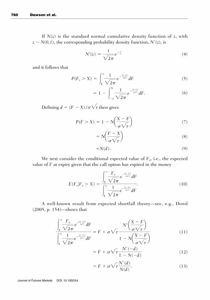
If N(z) is the standard normal cumulative density function of z, with z � N(0,1), the corresponding probability density function, N�(z), is

(4)

and it follows that

(5)

(6)

Defining then gives

(7)

(8)

(9)

We next consider the conditional expected value of F, i.e., the expectedvalue of F at expiry given that the call option has expired in the money

(10)

A well-known result from expected shortfall theory—see, e.g., Dowd(2005, p. 154)—shows that

(11)

(12)

(13)� F � s2tN�(d)N(d)

.

� F � s2tN�(�d)

1 � N(�d)

��

X

Ft

22pe�

(X � F)2

2s2t dF

��

X

1

22pe�

(X � F)2

2s2t dF

� F � s2t

N�aX � F

s2tb

1 � NaX � F

s2tb

E(Ft 0Ft � X) �

��

X

Ft

22pe�

(X � F)2

2s2t dF

��

X

1

22pe�

(X � F)2

2s2t dF

.

�N(d).

� NaF � X

s2tb

P(F � X) � 1 � NaX � F

s2tb

d � (F � X)�s2t

� 1 � �X

��

1

22pe

�(X�F)2

2s2t dF.

P(Ft � X) � ��

X

1

22pe�

(X�F)2

2s2t dF

N�(z) �1

22pe� z2

2

760 Dawson et al.




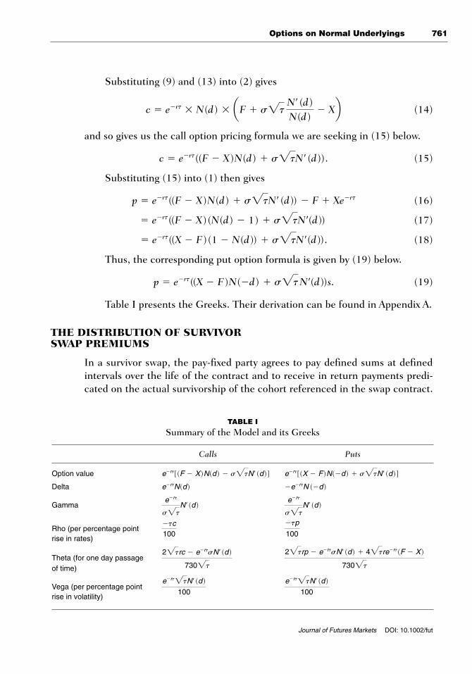
Substituting (9) and (13) into (2) gives

(14)

and so gives us the call option pricing formula we are seeking in (15) below.

(15)

Substituting (15) into (1) then gives

(16)

(17)

(18)

Thus, the corresponding put option formula is given by (19) below.

(19)

Table I presents the Greeks. Their derivation can be found in Appendix A.

THE DISTRIBUTION OF SURVIVOR SWAP PREMIUMS

In a survivor swap, the pay-fixed party agrees to pay defined sums at definedintervals over the life of the contract and to receive in return payments predi-cated on the actual survivorship of the cohort referenced in the swap contract.

p � e�rt((X � F)N(�d) � s2tN�(d))s.

� e�rt((X � F)(1 � N(d)) � s2tN�(d)).

� e�rt((F � X)(N(d) � 1) � s2tN�(d))

p � e�rt((F � X)N(d) � s2tN�(d)) � F � Xe�rt

c � e�rt((F � X)N(d) � s2tN�(d)).

c � e�rt � N(d) � aF � s2tN�(d)N(d)

� Xb

TABLE I

Summary of the Model and its Greeks

Calls Puts

Option value

Delta

Gamma

Rho (per percentage point rise in rates)

Theta (for one day passage of time)

Vega (per percentage point rise in volatility)

e�rt2tN�(d)

100

e�rt2tN�(d)

100

22trp � e�rtsN�(d) � 42tre�rt(F � X)

7302t

22trc � e�rtsN�(d)

7302t

�tp

100�tc100

e�rt

s2tN�(d)

e�rt

s2tN�(d)

�e�rtN (�d)e�rtN(d)

e�rt[(X � F)N(�d) � s2tN�(d)]e�rt[(F � X)N(d) � s2tN�(d)]

Lack of market completeness means that survivor swap contracts cannot bepriced with the zero-arbitrage methodology observed in interest rate swaps.Instead, a survivor premium, p, is factored into the payments of the pay-fixedparty. In the example cited later in this study, the pay-fixed party pays$K � (1 � p) on each anniversary for the number of members of a pre-definedcohort expected at the date of trading the swap to survive until that anniversaryand receives in return $K for every actual cohort survivor at that anniversary.Thus, a pension provider can turn an unknown survivorship liability into aseries of fixed payments. p is effectively the price of the survivor swap. p canbe positive or negative, depending on which party is observed to be at greaterrisk; p is also volatile.

Now let l(s, t, u) be the probability-based information available at s that anindividual who is alive at t survives to u. It follows that for each s � 1, . . . , t,we get

(20)

where (s) is the longevity shock in year s (Dowd et al., 2006, p. 5). This means that the probability of survival to t is affected by each of the one-yearlongevity shocks (1), (2), . . . , (t). Dowd (2005, p. 5) then suggests that the longevity shocks (1), (2), . . . , (t). can be modeled by the followingtransformed b distribution

(21)

where y(s) is b-distributed. As the b is defined over the domain [0, 1], the trans-formed b (s) is distributed over domain [�1, �1], where (s) � 0 indicatesthat longevity unexpectedly improved, and (s) � 0 indicates the opposite.

The premium p is set so that the initial value of the swap is zero, and, inthe case of a the simple vanilla swaps considered in Dowd et al. (2006), thisimplies that

(22)

where is the value of the fixed leg and is the value of thefloating leg, and li is the probability of survival to i. Equation (22) tells us that,in general, the swap premium is related to a weighted average of the expecta-tion of n � 1 independent (i) shocks, each of which follows a transformed b distribution. So what is the distribution of p?

The first point to note is that the average of n � 1 independent and identi-cally distributed shocks falls under the domain of the central limit theorem: this

qn�1

i�tliEq

n�1

i�tl1�e(i)i

p �

Eqn�1

i�tl1�e(i)i

qn�1

i�tli

� 1

e(s) � 2y(s) � 1

l(s, t � 1, t) � l(s � 1, t � 1, t)1�e(s)

762 Dawson et al.




immediately tells us that the distribution of p tends to normality as n gets large.In the present case, n is the number of years ahead over which the relevant sur-vivor rate is specified, so n realistically might vary from 1 to the time that thecohort concerned has completely died out (and this might be around 50 yearsfor a cohort of current age 65). Hence, we can say at this point that p tends toapproach normality as n gets large, but (especially for low value of n) the approx-imation to normality may be limited, depending on the distribution of (i).

This takes us to the distribution of (i) itself. In their original study, Dowdet al. (2006) suggested that the size of p reflected projected longevity improve-ments since the time that the pre-set leg of the swap was initially set. In thepast, the pre-set leg would typically have been based on projections from a mor-tality table that was prepared years before and projected fairly small mortalityimprovements. By contrast, the floating leg would be set by, say, the output of arecently calibrated stochastic mortality model that might have projectedstronger mortality improvements. However, as time goes by, we would expect all“views” of future mortality to be generated by reasonably up-to-date models,and differences of views would become fairly small. Hence, we would expect pto decline over time as swap counterparties become more sophisticated.

If we accept this line of reasoning, then the sets of b distribution parame-ters presented in Table 1 of Dowd et al. (2006) lead us to believe that the mostplausible representation of mortality given in that Table is their case 1: this iswhere (i) has a zero mean and a standard deviation of around 2.2%, and thisoccurs where the b distribution has parameters a � b � 1,000. Thus, if weaccept this example as plausible,3 we might expect the parameters of the b dis-tribution to be both high and approximately equal to each other. This is con-venient, because statistical theory tells us that a b distribution with a � b tendsto normality as a � b gets large (see, e.g., Evans, Hastings, & Peacock, 2000, p. 40). Thus, if we choose a and b to be large and equal (e.g., 1,000), then (i)will be approximately normal.

We therefore have two mutually reinforcing reasons to believe that the dis-tribution of premia might be approximately normal.

A PRACTICAL APPLICATION: PRICING SURVIVOR SWAPTIONS

As noted earlier, a practical illustration of the usefulness of this option pricingmodel can be found in the pricing of survivor swaptions. A survivor swaption

3We emphasize that this model is limited insofar as it assumes that mortality shocks are drawn from a single,age-independent, distribution. This is a convenient assumption for our illustrative purposes, and is compara-ble to the flat term structure often assumed in option pricing models. For a more general model, which allowsfor age-dependent shocks, see Cairns (2007) and Dawson et al (2008).

gives the right, but not the obligation, to enter into a survivor swap contract ata specified rate of p. The term p is also a risk premium reflecting the potentialerrors in the expectation of mortality evolution and p can be positive or nega-tive, depending on whether greater longevity (p � 0) or lower longevity(p � 0) is perceived to be the greater risk. It will also be zero in the case wherethe risks of greater and lower longevity exactly balance. Survivor swaptions can take one of two forms: a payer swaption, equivalent to our earlier call, inwhich the holder has the right but not the obligation to enter into a pay-fixedswap at the specified future time; and a receiver swaption, equivalent to ourearlier put, in which the holder has the right but not the obligation to enterinto a receive-fixed swap at the specified future time.

In order to price the swaption using the usual dynamic hedging strategiesassumed for pricing purposes, we are also implicitly assuming that there is aliquid market in the underlying asset, the forward survivor swap. Although werecognize that this assumption is not currently valid in practice, we woulddefend it as a natural starting point, not least because survivor swaptions can-not exist without survivor swaps.

We now consider an example calibrated on swaptions that mature in fiveyears’ time and are based on a cohort of U.S. males who will be 70 when theswaptions mature. The strike price of the swaption is a specified value of p andfor this example, we shall use an at-the-money forward option, i.e., X is set atthe prevailing level of p for the forward contract used to hedge the swaption.Setting the option to be at-the-money forward means that the payer swaptionpremium and the receiver swaption premium are identical.

Using the same mortality table as Dowd et al. (2006), and assuming, asthey did, longevity shocks, (i), drawn from a transformed b distribution withparameters 1,000 and 1,000 and a yield curve flat at 6%, Monte Carlo analysiswith 10,000 trials shows the moments of the distribution of p for the forwardswap to have the following values:

Mean 0.001156Annual variance 0.000119Skewness 0.008458Kurtosis 3.029241

The distribution is shown in Figure 1.A Jarque–Bera test on these data gives a test statistic value of 0.476. Given

that the test statistic has a x2 distribution with two degrees of freedom, this testresult is consistent with the longevity shocks following a normal distribution.

Figure 2 shows the options premia for both payer and receiver swaptionsacross p values spanning �3 standard deviations from the mean. The g, or con-vexity, familiar in more conventional option pricing models is also seen here.

764 Dawson et al.




As with conventional interest rate swaptions, the premia are expressed inpercentage terms. However, whereas with interest rate swaptions, the premiaare converted into currency amounts by multiplying by the notional principal,with survivor swaptions, the currency amount is determined by multiplying thepercentage premium by in which N is the cohort size,Aexpiry,t is the discount factor applying from option expiry until time t, K(t) is thepayment per survivor due at time t, S(t) is the proportion of the original cohortexpected to survive until time t, such expectation being observed at the time ofthe option contract, and where all members of the cohort are assumed to bedead after 50 years.4 is known with certainty at the timeof option pricing.

Figure 3 shows the changing value of the at-the-money forward payer andreceiver swaptions as time passes. The rapid price decay as expiry approaches,again familiar in more conventional options, is also seen here.

TESTING THE MODEL

The derivation of the model is predicated on the assumption that implementa-tion of a dynamic hedging strategy will eliminate the risk of holding long orshort positions in such options. We test the effectiveness of this strategy by

Ng50t�1Aexpiry,tK(t)S(t)

Ng50t�1Aexpiry,tK(t)S(t)

�0.1 0.0 0.1

0

50

100

150

200

250

300

350

400

450

Fre

quen

cy

�

FIGURE 1Distribution of the values of the p for a 45 year survivor swap starting in five

years’ time, from a Monte Carlo simulation of 10,000 trials with (i) values drawnfrom a transformed b distribution with parameters (1,000; 1,000). A normal

distribution plot is superimposed.

4This approach is equivalent to that used in the pricing of an amortizing interest rate swap, in which thenotional principal is reduced by pre-specified amounts over the life of the swap contract.

766 Dawson et al.


0.000%

0.500%

1.000%

1.500%

2.000%

2.500%

3.000%

�3.15%

�2.72%

�2.28%

�1.84%

�1.41%

�0.97%

�0.54%

�0.10%

0.33%

%

0.77%

1.20%

1.64%

2.08%

2.51%

2.95%

3.38%P

rem

ium

Payer Receiver

FIGURE 2Premia for the specified survivor swaptions.

0.0000%

0.1000%

0.2000%

0.3000%

0.4000%

0.5000%

0.6000%

0.7000%

0.8000%

5 4.5 4 3.5 3 2.5 2 1.5 1 0.5 0

Years to expiry

Pre

miu

m

FIGURE 3Options premia against time.



simulating the returns to dealers with (separate) short5 positions in payer andreceiver swaptions, and who undertake daily rehedging over the five year(1,250 trading days) life of the swaptions. We use Monte Carlo simulation tomodel the evolution of the underlying forward swap price, assuming a normaldistribution. We assume a dealer starting off with zero cash and borrowing or depositing at the risk-free rate in response to the cash flows generated by thedynamic hedging strategy. As Merton (1973, p. 165) states, “Since the portfoliorequires zero investment, it must be that to avoid ‘arbitrage’ profits, the expected(and realized) return on the portfolio with this strategy is zero.” Merton’s modelwas predicated on rehedging in continuous time, which would lead to expectedand realized returns being identical. In practice, traders are forced to use dis-crete time rehedging, which is modeled here. One consequence of this is that on any individual simulation, the realized return may differ from zero, but thatover a large number of simulations, the expected return will be zero. This isactually a joint test of three conditions:

1. The option pricing model is correctly specified—Equations (15) and (19)above;

2. The hedging strategy is correctly formulated—Equations (A1) and (A2)below, and

3. The realized volatility of the underlying asset price matches the volatilityimplied in the price of the option. We can isolate this condition by fore-casting results when this condition does not hold and comparing obser-vation with forecast. The dealer who has sold an option at too low an impliedvolatility will expect a loss, whereas the dealer sells at too high an im-plied volatility can expect a profit. This expected profit or loss of the dealer’sportfolio, E[Vp], at option expiry is

(23)

(24)

in which simplied and sactual represent, respectively, the volatilities implied inthe option price and actually realized over the life of the option.

We have conducted simulations across a wide set of scenarios, using dif-ferent values of p, simplied and sactual and different degrees of moneyness. In allcases, we ran 250,000 trials and in all cases, the results were as forecast. Byway of example,6 we illustrate in Table II the results of the trials of the option

�2rN�(d)(simplied � sactual)

E[Vp] � sert 0c0simplied

(simplied � sactual)

5The returns to long positions will be the negative of returns to short positions.6Results of the full range of Monte Carlo simulations are available on request from the corresponding author.

illustrated in Figures 1 and 2. The t-statistics relate to the differences betweenthe observed and the forecast mean outcomes.

The reader will note that the differences between the observed and expectedmeans are very low and statistically insignificant. This reinforces our assertionthat the model provides accurate swaption prices.

CONCLUSION

Interest in survivor derivatives from both the academic and practitioner commu-nities has grown rapidly in recent times, partly because of the economic impor-tance involved in the risk being managed and partly because of the significantintellectual challenges of developing such products. Trading in such derivativesis in its early stages and has largely been confined to linear payoff products.Option-based products seem inevitable and, given the normal distribution of therandom variable, p, used in the Dowd et al. (2006) survivor swap pricingmethodology, a model for pricing options on normally distributed assets isrequired. The model derived in this study is a straightforward adaptation of theBlack–Scholes–Merton approach and provides a robust solution to this problem.

APPENDIX A: DERIVATION OF THE GREEKs

Delta (�c, �p)The option’s �s follow immediately from (17) and (21)

(A1)

(A2)¢p �0p0F

� �e�rtN(�d).

¢c �0c0F

� e�rtN(d).

768 Dawson et al.


TABLE II

Results of Monte Carlo Simulations of Delta Hedging Strategy

Payer Receiver

Expected Standard Standard simplied sactual Value Mean Deviation Expected Mean Deviation (%) (%) (%) (%) (%) t-Stat Value (%) (%) (%) t-Stat

1.088998 1.088998 0.0000 0.0002 0.2092 0.40 0.0000 0.0002 0.2036 0.421.088998 0.988998 0.0892 0.0894 0.1897 0.45 0.0892 �0.0894 0.1853 0.461.088998 1.188998 �0.0892 �0.0891 0.2287 0.24 �0.0892 �0.0891 0.2221 0.24

Note. Simulations carried out using @Risk, with 250,000 trials.



Gamma( c, p)

(A3)

(A4)

(A5)

(A6)

(A7)

(A8)

(A9)

Rho (Pc, Pp)

(A10)

(A11)

Theta (�c, �p)

(A12)

By the product rule

(A13)

(A14)

(A15)

(A16)

(A17)(A18)� �rc

� �re�rt[(F � X)N(d) � s2tN�(d)]

A � [(F � X)N(d) � s2tN�(d)]00t

e�rt

... 0c0t

� A � B.

Let B � e�rt00t

[(F � X)N(d) � s2tN�(d)]

Let A � [(F � X)N(d) � s2tN�(d)]00te�rt.

� e�rt 00t

[(F � X)N(d) � s2tN�(d)].

0c0t

� [(F � X)N(d) � s2tN�(d)]00t

e�rt

0c0t

�00t

e�rt[(F � X)N(d) � s2tN�(d)].

Pp �0p0r

� �tp.

Pc �0c0r

� �tc.

�e�rt

s2tN�(d)

�e�rt

s2tN�(�d)

�e�rt0(�d)0F

�0N(�d)0d

p �02p0F2 �

0¢p

0F� �

0e�rtN(�d)0F

�e�rt

s2tN�(d).

� e�rt 0d0F

�0N(d)0d

c �02c0F2 �

0¢c

0F�0e�rtN(d)0F

(A19)

Applying the sum rule

(A20)

(A21)

(A22)

(A23)

The chain rule then implies

(A24)

(A25)

(A26)

By the product rule

(A27)

(A28)

(A29)

(A30)

(A31)

By the chain rule

(A32)F � e�rts2t00t

N�(d) � e�rts2t00d

N�(d)0d0t

... 0c0t

� �rc �e�rtd(F � X)N�(d)

2t�

e�rtsN�(d)

22t� F.

E � e�rtN�(d)00ts2t �

e�rtsN�(d)

22t

Let F � e�rts2t00tN�(d).

Let E � e�rtN�(d)00ts2t.

D � e�rt 00ts2tN�(d) � e�rtN�(d)

00ts2t � e�rts2t

00t

N�(d).

... 0c0t


2t� D.

� �e�rt d(F � X)N�(d)

2t

C � e�rt(F � X)00t

N(d) � e�rt(F � X)00d

N(d)0d0t

... 0c0t

� �rc � C � D.

Let D � e�rt00ts2tN�(d)

Let C � e�rt(F � X)00tN(d).

� e�rt(F � X)00t

N(d) � e�rt 00ts2tN�(d).

B � e�rt 00t

[(F � X)N(d) � s2tN�(d)]

...0c0t

� �rc � B.

770 Dawson et al.




(A33)

(A34)

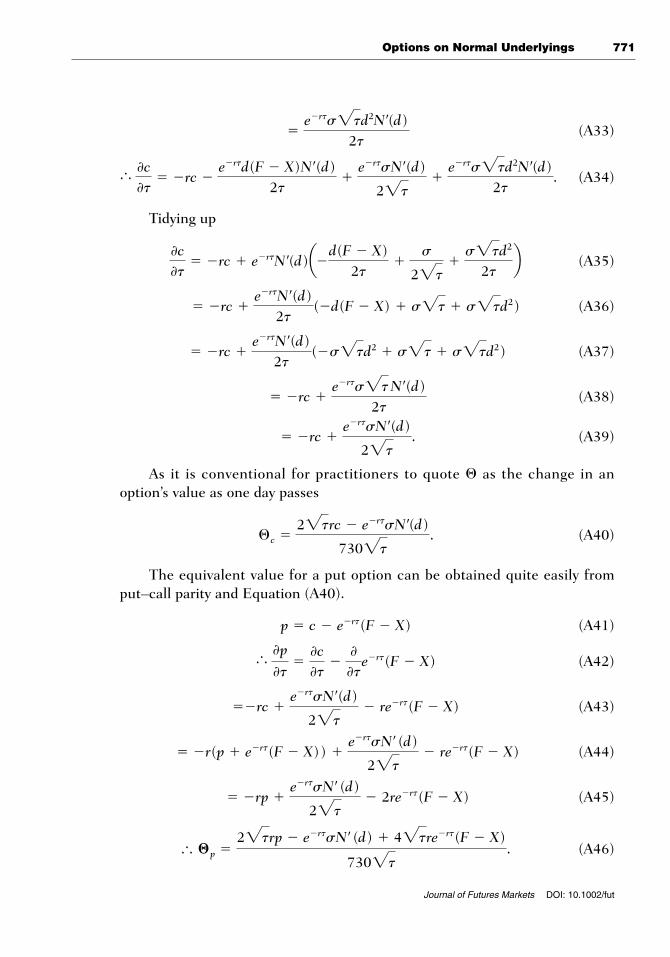
Tidying up

(A35)

(A36)

(A37)

(A38)

. (A39)

As it is conventional for practitioners to quote � as the change in anoption’s value as one day passes

(A40)

The equivalent value for a put option can be obtained quite easily fromput–call parity and Equation (A40).

(A41)

(A42)

(A43)

(A44)

(A45)

(A46)... ∏p �22trp � e�rtsN�(d) � 42tre�rt(F � X)

7302t.

� �rp �e�rtsN�(d)

22t� 2re�rt(F � X)

� �r(p � e�rt(F � X) ) �e�rtsN�(d)

22t� re�rt(F � X)

��rc �e�rtsN�(d)

22t� re�rt(F � X)

...0p0t

�0c0t

�00t

e�rt(F � X)

p � c � e�rt(F � X)

®c �22trc � e�rtsN�(d)

7302t.

� �rc �e�rtsN�(d)

22t

� �rc �e�rts2tN�(d)

2t

� �rc �e�rtN�(d)

2t(�s2td2 � s2t � s2td2)

� �rc �e�rtN�(d)

2t(�d(F � X) � s2t � s2td2)

0c0t

� �rc � e�rtN�(d)a�d(F � X)2t

�s

22t�s2td2

2tb

... 0c0t


2t�

e�rtsN�(d)

22t�

e�rts2td2N�(d)2t

.

�e�rts2td2N�(d)

2t

Vega

(A47)

(A48)

(A49)

(A50)

(A51)

By the chain rule

(A52)

(A53)

(A54)

By the product and chain rules

(A55)

(A56)

(A57)

(A58)

(A59)

As practitioners generally present vega in terms of a one percentage pointchange in volatility, we present vega here as

(A60)0c0s

�e�rt2tN�(d)

100.

� e�rt2tN�(d).

... 0c0s

� e�rt2t(d2 � 1)N�(d) � e�rt2td2N�(d)

� e�rt2t(d2 � 1)N�(d)

� e�rtN�(d)2t � e�rts2tN�(d)d2

s

H � e�rt 00ss2tN�(d) � e�rtN�(d)

00ss2t � e�rts2t

00d

N�(d)0d0s

� �e�rt2td2N�(d).

��e�rtd(F � X)N�(d)

s

G � e�rt(F � X)00s

N(d) � e�rt(F � X)00d

N(d)0d0s

0c0s

� G � H.

Let H � e�rt00ss2tN�(d).

Let G � e�rt(F � X)00sN(d).

� e�rt(F � X)00s

N(d) � e�rt 00ss2tN�(d).

0c0s

�00s

e�rt[(F � X)N(d) � s2tN�(d)]

a 0c0s

,0p0sb

772 Dawson et al.




Put–call parity shows that the vega of a put option equals the vega of a calloption

(A61)

(A62)

BIBLIOGRAPHY

Bachelier, L. (1900). Théorie de la spéculation. Paris: Gauthier-Villars.Bauer, D., & Kramer, F. W. (2008). Risk and valuation of mortality contingent catas-

trophe bonds, Pensions Institute (Discussion Paper PI-0805).Bauer, D., & Russ, J. (2006). Pricing longevity bonds using implied survival probabilities.

(Available at http://www.mortalityrisk.org/Papers/Models.html).Black, F., & Scholes, M. (1973). The pricing of options and corporate liabilities.

Journal of Political Economy, 81, 637–654.Blake, D., Cairns, A., & Dowd, K. (2006). Living with mortality: Longevity bonds and

other mortality-linked securities. British Actuarial Journal, 12, 153–228.Blake, D., Cairns, A., & Dowd, K. (2008). The birth of the life market. Asia-Pacific

Journal of Risk and Insurance, 3(1), 6–36.Blake, D., Cairns, A., Dowd, K., & MacMinn, R. (2006) Longevity bonds: Financial

engineering, valuation and hedging. Journal of Risk and Insurance, 73, 647–672.Cairns, A. J. G., (2007). A multifactor generalisation of the Olivier-Smith model for

stochastic mortality. In Proceedings of the First IAA Life Colloquium, Stockholm,2007.

Cairns, A., Blake, D., & Dowd, K. (2008). Modelling and management of mortality risk:A review. Scandinavian Actuarial Journal, forthcoming.

Carmona, R., & Durrleman, V. (2003). Pricing and hedging spread options. SIAMReview, 45, 627–685.

Cox, J. C., & Ross, S. A. (1976). The valuation of options for alternative stochasticprocesses. Journal of Financial Economics, 3, 145–166.

Dahl, M., & Møller, T. (2005). Valuation and hedging of life insurance liabilities withsystematic mortality risk. In Proceedings of the 15th international AFIR colloquium.Zurich. (Available at http://www.a_r2005.ch).

Dawson, P., Dowd, K., Cairns, A. J. G., & Blake, D. (2008). Completing the market forsurvivor derivatives: A general pricing framework. Pensions Institute (DiscussionPaper PI–0712).

Dowd, K. (2005). Measuring market risk (2nd ed.). New York: Wiley.Dowd, K., Cairns, A. J. G., Blake, D., & Dawson, P. (2006). Survivor swaps. Journal of

Risk and Insurance, 73, 1–17.Evans, M., Hastings, N., & Peacock, B. (2000). Statistical distributions (3rd ed.).

New York: Wiley.Haug, E. G. (2006). Complete guide to option pricing formulas. New York: McGraw-Hill.JPMorgan. (2007). LifeMetrics: A toolkit for measuring and managing longevity and

mortality risks (Available at http://www.lifemetrics.com/).

...0p0s

�0c0s

�00s

e�rt(F � X) �0c0s

.

p � c � e�rt(F � X)

Merton, R. C. (1973). Theory of rational option pricing. Bell Journal of Economics andManagement Science, 4, 141–183.

Sherris, M., & Wills, S. (2007). Financial innovation and the hedging of longevity risk.Presented at the third international longevity risk and capital market solutionssymposium. Taipei, July.

Wills, S., & Sherris, M. (2008). Securitization, structuring and pricing of longevity risk,Pensions Institute (Discussion Paper PI-0816).

774 Dawson et al.


options on normal underlyings with an application to the pricing of survivor swaptions

Documents