option pricing in the presence of liquidity risk
TRANSCRIPT

Option Pricing in the Presenceof Liquidity Risk
Author: Martin Harr∗
Department of Physics, Umea UniversitySE-90187 Umea, Sweden
Supervisor: Kaj NystromMaster of Science in Engineering Physics
July 9, 2010
∗Email: [email protected]

Abstract
The main objective of this paper is to prove that liquidity costs do exist in option pric-ing theory. To achieve this goal, a martingale approach to option pricing theory is usedand, from a model by Jarrow and Protter [JP], a sound theoretical model is derived toshow that liquidity risk exists. This model, derived and tested in this extended theory,allows for liquidity costs to arise. The expression liquidity cost is used in this paper tomeasure liquidity risk relative to the option price.
The approach to show that there exist liquidity costs is carried out in two steps. Thefirst step is to derive a model built on a theoretical model derived by Jarrow and Prot-ter, and the second step is to use the model to attain the size of this cost, in this caserelative to the option price.
The model uses a supply curve to account for the supply/demand in the market. Thesupply curve is integrated into the model and is also proven to exist, both in theory andin practice. To show how non horizontal supply curve affect option prices simulationsare made using MATLAB. The impact of liquidity risk is presented as a percentage ofthe analytical option price.
The result show a real liquidity risk, although small, that can have a big impact insystems with a big turnover in options, i.e. financial institute, and also in a crisis whenthe supply curve is changed and has a bigger impact on the option price. In a ”normal”case the liquidity costs is in the order of 10−2 to 10−3 percent of the option prices.
This paper uses the recent advances concerning the including liquidity risk of optionpricing theory [JP]. Here new insights into the relevance of the classical techniques usedin ’continuous time finance for practical risk management’ are tested. The First andSecond Fundamental Theorem are proven valid for this extension of the theory. Dif-ferent supply curve models of liquidity issues in stock and option market trading arediscussed.
Keywords and phrases: liquidity risk, liquidity costs, option theory, supply curve, mar-tingale approach in option pricing.
Sammanfattning
Huvudsyftet med denna uppsats ar att visa att likviditetsrisk existerar i optionsvarderingsteorin.For att uppna detta mal anvands en martingal ansats vid optionsprissattning for attastadkomma en hallbar teoretisk modell och bygger pa en modell Jarrow och Protterhar tagit fram [JP]. Modellen byggs och testas i denna utokade teori for att visa attlikviditetskostnader uppstar. Uttrycket likviditetskostnad anvands i denna uppsats fratt kunna mata likviditetsrisk i forhallande till optionspriset.
Den har uppsatsen anvander tva steg for att bevisa att likviditetskostnader vid op-tionsprissattning existerar. Forsta steget ar att ta fram en modell som bygger pa enmodell som Jarrow och Protter utvecklat och det andra steget ar att anvanda modellenoch ta fram en storlek pa denna kostnad i forhallande till optionspriset.
Den framtagna modellen anvander sig av utbudskurvan for att ta hansyn till tillgangoch efterfragan pa marknaden. Utbudskurvan ar integrerad i modellen och det ar be-visat att den existerar i teori och praktik. Simuleringar ar utforda pa den framtagnamodellen for att visa hur likviditetskostnader paverkar optionspriset. Effekterna av lik-viditetsrisk presenteras som en procentandel av det analytiska optionspriset.
Resultatet visar en verklig likviditetsrisk som ar liten men kan ha en stor inverkani system med en stor omsattning i optioner, till exempel finansiella institut, och aveni en kris nar utbudskurvan andras och har en storre inverkan pa optionspriset. I ”nor-mal” fallet ligger likviditetskostnaden storleksmassigt mellan 10−2 och 10−3 procent avoptionspriset.
Denna uppsats anvander de senaste framstegen inom likviditetsrisk i optionsvarderingsteorin.Har testas betydelsen av klassiska tekniker som anvands i praktisk riskhantering i kon-tinuerlig tid. Det Forsta och Andra Fundamentala Teoremet inom optionsprissattningvisar sig halla i den har utokade teorin. Olika utbudskurvor diskuteras kring lik-viditetsfragor vid handel pa vardepappersmarknader.
Nyckelord och fraser: likviditetsrisk, likviditetskostnader, optionsteori, utbudskurva, mar-tingal ansats vid optionsprissattning.

Contents
1 Introduction 11.1 Background . . . . . . . . . . . . . . . . . . . . . . . . . . . . . . . . . . . . . 11.2 Purpose . . . . . . . . . . . . . . . . . . . . . . . . . . . . . . . . . . . . . . . 11.3 Limitations . . . . . . . . . . . . . . . . . . . . . . . . . . . . . . . . . . . . . 21.4 Objectives . . . . . . . . . . . . . . . . . . . . . . . . . . . . . . . . . . . . . . 21.5 Theoretical Introduction . . . . . . . . . . . . . . . . . . . . . . . . . . . . . . 31.6 Heuristic Explanation of Conceptions . . . . . . . . . . . . . . . . . . . . . . . 4
2 Liquidity and Options 52.1 Liquidity Risk . . . . . . . . . . . . . . . . . . . . . . . . . . . . . . . . . . . . 52.2 Basic Option Theory . . . . . . . . . . . . . . . . . . . . . . . . . . . . . . . . 62.3 Basic Option Theory with the Martingale Approach . . . . . . . . . . . . . . . 7
3 The Model 103.1 Market-to-Market Value and Liquidity Costs . . . . . . . . . . . . . . . . . . . 113.2 The First Fundamental Theorem . . . . . . . . . . . . . . . . . . . . . . . . . 123.3 The Fictitious Economy . . . . . . . . . . . . . . . . . . . . . . . . . . . . . . 133.4 Contingent Claim . . . . . . . . . . . . . . . . . . . . . . . . . . . . . . . . . . 13
3.4.1 Example of Contingent Claim . . . . . . . . . . . . . . . . . . . . . . . 143.5 Market Completeness . . . . . . . . . . . . . . . . . . . . . . . . . . . . . . . . 143.6 The Second Fundamental Theorem . . . . . . . . . . . . . . . . . . . . . . . . 163.7 Example of an Economy with Liquidity Risk . . . . . . . . . . . . . . . . . . . 17
4 Economies with Supply Curves for Derivatives 194.1 Discrete Trading Strategies . . . . . . . . . . . . . . . . . . . . . . . . . . . . . 194.2 Transactional Costs . . . . . . . . . . . . . . . . . . . . . . . . . . . . . . . . . 21
4.2.1 Fixed Transaction Costs . . . . . . . . . . . . . . . . . . . . . . . . . . 214.2.2 Proportional Transaction Costs . . . . . . . . . . . . . . . . . . . . . . 224.2.3 Combined Fixed and Proportional Transaction Costs . . . . . . . . . . 22
4.3 Linear Supply Curves . . . . . . . . . . . . . . . . . . . . . . . . . . . . . . . . 22
5 Method 255.1 Supply Curve . . . . . . . . . . . . . . . . . . . . . . . . . . . . . . . . . . . . 255.2 Derivatives . . . . . . . . . . . . . . . . . . . . . . . . . . . . . . . . . . . . . . 265.3 Liquidity Costs . . . . . . . . . . . . . . . . . . . . . . . . . . . . . . . . . . . 275.4 Empirical Liquidity Costs . . . . . . . . . . . . . . . . . . . . . . . . . . . . . 27
6 Result 296.1 Theoretical Supply Curve . . . . . . . . . . . . . . . . . . . . . . . . . . . . . 29
6.1.1 Liquidity Cost Sensitivity . . . . . . . . . . . . . . . . . . . . . . . . . 306.1.2 Risk Free Rate Sensitivity . . . . . . . . . . . . . . . . . . . . . . . . . 316.1.3 Volatility Sensitivity . . . . . . . . . . . . . . . . . . . . . . . . . . . . 316.1.4 Spot Price Sensitivity . . . . . . . . . . . . . . . . . . . . . . . . . . . . 326.1.5 Strike Price Relative Spot Price Sensitivity . . . . . . . . . . . . . . . . 326.1.6 Supply Curve Slope Sensitivity . . . . . . . . . . . . . . . . . . . . . . 32

6.1.7 Supply Curve Bid Ask Spread Sensitivity . . . . . . . . . . . . . . . . . 336.1.8 Timestep Sensitivity . . . . . . . . . . . . . . . . . . . . . . . . . . . . 336.1.9 Time to Maturity Sensitivity . . . . . . . . . . . . . . . . . . . . . . . . 336.1.10 Worst Case Scenario . . . . . . . . . . . . . . . . . . . . . . . . . . . . 33
6.2 Empirical Supply Curve . . . . . . . . . . . . . . . . . . . . . . . . . . . . . . 34
7 Conclusions 357.1 Theory . . . . . . . . . . . . . . . . . . . . . . . . . . . . . . . . . . . . . . . . 357.2 Result . . . . . . . . . . . . . . . . . . . . . . . . . . . . . . . . . . . . . . . . 35
8 References 37

1 Introduction
1.1 Background
Issues of liquidity have long been discussed between stock and option traders. If there is agiven hedging strategy, the profit can be reduced by liquidity costs due to updating positionsin the strategy. This liquidity costs should be included into the price one charges for theoption. When calculating an option price, the price movement of the underlying asset to thematurity date has to be estimated.
Grossman and Miller [GM] in 1988 presented a supply and demand equilibrium approachto this problem. Perhaps liquidity in the stock market never could be precisely defined, butthere should exist some kind of relation between price and size of order. This is the attitude ofpractitioners and academics alike. In the following a more modern approach of arbitrage freepricing is discussed, which has the benefit of allowing more explicit and detailed calculations.
In the approach presented here the existence of a supply curve is postulated as a new keyfeature of the option pricing theory. This theory is a relatively simple solution to issues ofliquidity. It has been showed that a supply curve actually exists and is not just a line withslope zero. [CJP]
1.2 Purpose
Liquidity risk in option pricing is a fairly new area of research and is up to today mainly basedon the experience of practitioners. Many of the results in this area are heuristic. Even thoughthere has been some recent progress in the research concerning liquidity risk research thereare still quite few mathematical approaches to liquidity risk modeling. This is partly due toquite sophistical level of mathematics involved in this type of theory. The main purpose ofthis paper is to derive a sound option pricing model using the approach developed by Jarrowand Protter [JP] and to show the impact of liquidity risk by constructing a simulation tool.Simulation techniques have been successfully applied in financial mathematics but there doesnot exist a simulation tool for this specific case, when liquidity costs is taken into account inthe option price.
The main focus is to work with existing theory in this field and derive a sound model, i.e.extending the already existing theory in option pricing, and base the model on the theoryJarrow and Protter have developed in this research area [JP]. This theory is then used tobuild a model of the extended economy.The model is then used to investigate if the liquidityrisk has an impact on the option price set by analytical solutions, or approximated analyticalsolutions. The option has the famous Black Scholes model as underlying factor when deriv-ing the price. The results presented in this paper are based on a theoretical sound, intuitionregarding supply curves, i.e. liquidity costs, and the results of other researchers.
1

1.3 Limitations
The simulation tool will be developed to test three different options and the specific put andcall types of these options, in total six different option types. The options used are chosen byhow common they are in the option market and to some extent, my own interest. All optionsare of the type European. The Black Scholes pricing model is used when deriving the optionprice. This is used only to normalize the liquidity risk by present the numbers in percent ofthe option price. To calculate liquidity costs a supply curve needs to be determined.
1.4 Objectives
The main objective is to derive a model using the sound extended theory by Jarrow and Prot-ter [JP], derived from the martingale approach to option theory and design a simulation toolto determine the impact liquidity costs have on the option price. This model is an extensionof previously work done by Jarrow and Protter in liquidity risk theory using a martingaleapproach for arbitrage pricing of options. To analyze the outcome of this result a simulationtool is used to view the size of this liquidity risk in options. The result from simulations isthen analyzed.
To sum up the objectives in this paper are:
1. Derive a model built on the work of Jarrow and Protter [JP] and show that liquidityrisk exist when pricing options,
2. Build a simulation tool, i.e. a model of this extended theory, using the computer programMATLAB and apply input data,
3. Analyze the results from this simulation tool, and the input data.
2

1.5 Theoretical Introduction
The article of Jarrow and Protter concerning liquidity risk [JP] summarizes the recent ad-vances on the inclusion of liquidity risk into option pricing theory. Classical asset pricingtheory states that investors actions on the market has no impact on the price paid or re-ceived, traders act as price takers. Softening of the price due to this assumption and theimpact to the actual realized returns in asset pricing models is called liquidity risk.
Liquidity risk has been extensively studied in the market microstructure literature but notas extensively in asset pricing literature. The market microstructure literature states that abig impact on prices can be due to asymmetric information or difference in risk tolerance [K].Liquidity risk has been studied in an extreme case, market manipulation [CM]. The researchdone by Cetin [C] conclude that liquidity risk is related to transaction costs and therebyaffect the price paid or received.
This article uses the classical option pricing theory with embedded liquidity risk. The in-vestors act in this approach as price takers with respect to a C2 supply curve on the underlyingasset. [C]
Liquidity costs exist but are non-binding because no arbitrage opportunities can exist. Stillwith this extension appropriate generalizations of the First and Second Fundamental Theo-rem of asset pricing hold [CJP]. It can be stated that markets are arbitrage free if and onlyif there exists an equivalent martingale measure.
The supply curve must have discontinuity at 0 [C] or continuous trading strategies mustbe excluded to hold for the extended theory. Continuous trading strategies are not possiblein practice, only approximations of simple strategies are doable [CJPW]. For simple strate-gies liquidity costs are binding which implies that the market is no longer complete and anupward sloping supply curve for options can exist.
3
1.6 Heuristic Explanation of Conceptions
Here are some words given some heuristic definitions however to get rigorous statements andconcepts you are referred to Øksendal [O], Bjork [B] and Hull [H]. This is soft descriptionsof some concepts used in this paper to make it easier to read and understand without a deepknowledge in financial mathematics.
Arbitrage - A possibility to make a profit without taking any risk.Borel measure - Any measure µ defined on the σ-algebra of Borel sets is called a Borelmeasure.Brownian motion - A continuous-time stochastic process with properties W0 = 0, Wt isa.s. continuous function on [0, T ], has independent increments and Wt −Ws ∼ N (0, t − s)for any 0 ≤ s < t ≤ T .FLVR. - Free lunch with vanishing risk.Contingent claim - Derivative (option with cash settlement).Derivative - An agreement or contract that is not based on a real exchange, the real def-inition of a derivative is an agreement between two parties that is contingent on a futureoutcome of the underlying (option with cash settlement).Free lunch with vanishing risk - Defined mathematically as a ’softer’ no arbitrage defi-nition.Liquidity cost - The cost derived from liquidity risk, i.e. the premium you have to pay tofree the money you have locked up in for example stocks.Liquidity risk - Liquidity cost.Market-to-market value - the value of an asset based on the current market price of theasset, or for similar assets, or based on another objectively assessed fair value.Martingale - A stochastic process such that the conditional expected value of an observationat some time t, given all the observations up to some earlier time s, is equal to the observationat that earlier time s.Maturity - The final payment date of a loan or other financial instrument, at which pointthe principal (and all remaining interest) is due to be paid.Option - A contract between a buyer and a seller that gives the buyer of the option theright, but not the obligation, to buy or to sell a specified asset (underlying) on or before theoptions expiration time, at an agreed price, the strike price.Replicating portfolio - This is a fictitious portfolio used to evaluate the price of an optionby buying and selling the underlying asset.Supply curve - The curve explaining how the price depends on the size of a stock order.SFTS. - Self financing trading strategy.Self financing trading strategy - This is a trading strategy which generates no cash flowsfor all defined times and can be called a replicating portfolio. This portfolio borrows or in-vests in the money account to purchase or sell stocks.Semimartingale - It can be decomposed as the sum of a local martingale and an adaptedfinite-variation process.Supermartingale - A concave function of a martingale is a supermartingale, i.e. the expec-tation value decreases over time.
4

2 Liquidity and Options
Three different steps are used in this study. First a brief introduction in option theory ismade. This is done to allow the reader to understand the option pricing theory and also seethe problem in extending this to include liquidity risk. The next step is to derive a simpleand sustainable model based on a theoretical model by Jarrow and Protter [JP] which theliquidity risk are included and also proven to exist theoretically. After these steps the modelare simulated trough a data program called MATLAB. This is done to ensure that the theo-retical evidence also hold in practice.
The theory is presented by first defining liquidity risk and then describing what an op-tion is and how it is priced. This is done for the reader so that a natural discussion can bemade when deriving a sound theoretical framework. When liquidity risk and option pricing isdefined in a suitable way the economy is discussed with a model of the economy. The modelis defined and the market-to-market value and liquidity costs which arises in this model isdiscussed. The First Fundamental Theorem is tested in this economy and to test the SecondFundamental Theorem a breif introduction in the definition of a contingent claim (see theHeuristic Explanation of Conceptions for definition) is made. This definition is then testedin the assumption that the market is complete1 which leads to a formulation of the SecondFundamental Theorem is possible. Now examples of economies including liquidity risk canbe constructed. The examples presented has the objective to illustrate the difficulty to definea theoretical sound economy with liquidity risk. A possible definition of supply curves aremade and properties of such a supply curve is presented.
2.1 Liquidity Risk
There are two kinds of liquidity [P]: market liquidity, and funding liquidity. A security hasgood market liquidity if it is easy to trade, i.e. has a low bid ask spread, small price impact,high resilience and is easy to find in OTC markets. A bank or investor has good fundingliquidity if it has enough available funding from its own capital or from loans.
With these definitions the meaning of liquidity risk can be described. Market liquidity risk isthe risk that the market liquidity worsens when you need to trade. Funding liquidity risk iswhen a trader no longer has the funds to keep his position and is forced to reduce the position.An example is when a levered hedge fund loses the access to borrow from their bank and isforced to sell their holdings (securities) as a result. Another example is depositors to a bankmay withdraw their funds and the bank may lose the ability to borrow from other banks orraise funds through debt issues.
Liquidity generally varies over time and across markets. The most extreme form of mar-ket liquidity risk is that dealers are shutting down (no bids). Funding liquidity risk occurswhen banks are short on capital. When this is happening the banks are forced to scale backtheir trading that requires capital and the amount of capital they lend out, for example toother traders. If banks cannot fund themselves, they cannot fund their clients. The two forms
1A market is complete with respect to a trading strategy if there exists a SFTS. such that at any time t,the returns of the two strategies are equal.
5

of liquidity are linked and can reinforce each other in liquidity spirals where poor fundingleads to less trading. This reduces market liquidity, increasing margins and tightening riskmanagement to further worsening funding.
2.2 Basic Option Theory
Black and Scholes defined an option to be a security giving the right to buy/sell an asset un-der certain conditions within a specified period of time [BS]. An option is a contract betweena buyer and a seller that gives the buyer of the option the right, but not the obligation tobuy/sell a specified underlying asset on or before the options expiration date (maturity) atan agreed price (strike price).
There are lots of different types of options. A call option is an option that gives the right tobuy an underlying asset and a put option gives the right to sell the underlying asset.
Figure 1: Illustrate the option value before maturity.
An option has a value to the person who holds this option. The buyer of an option has to paya premium to the seller of the option and, consequently the right to buy or sell the underlyingasset. When an options maturity is reached the owner may choose to exercise the right tobuy or sell the asset. If in the case of a call option, the spot price is higher than the strikeprice, the option owner exercises the right to buy a predetermined amount of the underlyingasset and sell it on the market at market price at profit. If the option chooses to exercise thisright the seller of the option are obliged to sell the asset to the buyer (owner) of the optionat the strike price. [H]
A call option with a strike price much lower than the asset price is likely to be exercised. Theprobability in this case, not to exercise the option is very small and the value of the option isclose to the difference between the strike price and the spot price on the underlying asset. If
6

the strike price was much higher than the asset price the value of the option would be almostzero. The time remaining until maturity of an option also influence the value. If there isa long time until maturity the potential for the option to profitable for the buyer increaseswhich also gives a higher value. If the underlying assets price does not change over timethe value of the option drops as the maturity date comes closer which leads to a decrease inpotential for a profitable option for the buyer. [BS]
The option value can be divided into two parts, the intrinsic value and the time value.These two values interact and makes up the total value of an option. The intrinsic value isa non-negative value and is non-zero if the option has a payoff.
A European option is the right to buy or sell the underlying asset only at the maturitydate of the option. If these rights can be exercised at any time it is an American option.This value has different forms depending on which option you look at. Some different optiontypes are European option, Digital option, Asian option, Lookback option, Barrier option,Spread option and Basket option. [H]
2.3 Basic Option Theory with the Martingale Approach
The theoretical approach in this paper begins with the martingale approach to arbitrage the-ory. This is the most general approach existing for arbitrage pricing and is also very efficientfrom a computational point of view.
A filtered probability space is needed when using the martingale approach to pricing op-tions. Let (Ω,F , (Ft)0≤t≤T ,P).
The market model consists of N + 1 a priori2 given asset price processes S0, S1, ..., SN , inthis case the Black Scholes model. Fundamental problems occur under these conditions; un-der what conditions is the market arbitrage free and complete. These problems have thefamous solutions First and Second Fundamental Theorem of Mathematical Finance. Theseresults are general and powerful but also quite deep so in this section only the main structuralideas of the proofs are presented and follows the approach made by Bjork. [B]
Take a market model consisting of the asset price process S0, S1, ..., SN on the time interval[0, T ]. The numeraire process3 S0 is assumed to be strictly positive. Some simple assumptionsare made. A T-claim4 is fixed as R. Derivative instruments are completely defined in termsof the underlying asset S and can also be called contingent claims. The name, contingentclaim, is used in this paper.
FST -adapted means that for each fixed time T the process R is a functional of the Wienertrajectory on the interval [0, T ]. A T-claim R can be replicated, alternatively reachable or
2A priori knowledge is prior knowledge about a population, rather than that estimated by recent obser-vation.
3basic standard by which values are measured, in this case a normalized economy with S0 as a numeraire,relative price process S(t)/S0(t).
4A contingent claim with date of maturity T , or T-claim, is any stochastic variable R ∈ FST .
7
hedgeable, if there exists a self financing trading strategy (SFTS.) X such that
V X(T ) = R, in P a.s.
This means that X is a hedge, replicating portfolio or hedging portfolio against R.
To show that no arbitrage are possible and the market is complete, the First and SecondFundamental Theorem are stated. A normalized economy is used only to make the processeasier. It still holds for non-normalized economies.
Theorem 2.1 (First fundamental Theorem) The market model is free of arbitrage if andonly if there exists a martingale measure, a measure Q ∼ P, such that the processes
S0(t)
S0(t),S1(t)
S0(t), ...,
SN(t)
S0(t)
are (local) martingales under Q . [B]
To exemplify this consider the case where the numeraire S0(t) is the money account
S0(t) = e−∫ t0 r(u)du
where r is the (possible stochastic) short rate and if the assumption, that all process areWiener driven, are made then a measure Q ∼ P is a martingale measure if and only if allassets S0, S1, ..., SN have the short rate as their local rates of return, i.e. if the Q -dynamicsare of the form
dSi(t) = Si(t)r(t)dt+ Si(t)σi(t)dWQ(t),
where WQ is a (multidimensional) Q -Brownian motion. The second result is used as condi-tions for market completeness. σ is only a defined volatility.
Theorem 2.2 (Second fundamental Theorem) Assuming absence of arbitrage, the marketmodel is complete if and only if the martingale measure Q is unique. [B]
This summarizes the basic theory conserning pricing contingent claims. A consequence ofthis theorem is that in order to avoid arbitrage, R must be priced according to the formula
Γ(t;R) = S0(t)EQ[
R
S0(T )|Ft], (2.1)
where Q is a martingale measure for [S0, S1, ..., SN ], with S0 as the numeraire. If the bankaccount has W (t) as the numeraire then W (t) has the dynamics
dW (t) = r(t)W (t)dt,
where r is as before the short rate process. In this case the pricing formula above reduces to
Γ(t;R) = S0(t)EQ[e−
∫ t0 r(u)duR|Ft
].
8

Different Q could give different price processes for a fixed claim R, but if R is attainable thenall Q will produce the same price process and this price process is given by
Γ(t;R) = V (t;X),
where X is the hedging portfolio. Different choices of hedging portfolios (if such exist) willproduce the same price process. Especially, for every replicable claim X it holds that
V (t;X) = S0(t)EQ[e−
∫ t0 r(u)duR|Ft
].
Summing up the price of any derivative instrument in a complete market will be uniquelydetermined by the required no arbitrage. The price is unique because it can be replaced bythe replicating portfolio. The price on the derivative does not depend on the risk the brokersor agents in the market are willing to take. This means that they can have any attitudetowards risk as long as they prefer more (deterministic) money to less.
In an incomplete market the requirement of no arbitrage is no longer sufficient to determinea unique price for options. There are several martingale measures that can price derivativesin a no arbitrage economy. The price of a derivative using the martingale measure is chosenby the market and is determined by two major factors:
1. The derivative should be priced so that there are no arbitrage possibilities on the market.This requirement is derived from equation (2.1) where all derivatives use the same Q.
2. When there is an incomplete market the price also depends on the supply/demand on themarket. Supply and demand for a specific derivative depends on the aggregate risk aversionon the market, liquidity considerations and other factors. All these aspects are aggregatedinto a particular martingale measure used by the market. [B]
9

3 The Model
Let (Ω,F , (Ft)0≤t≤T ,P) be a filtered probability space satisfying usual conditions with T as afixed time. Lets consider a security in a market and call it a stock with no dividends. Thereis also a money market account that uses the spot rate of interest as return. Assuming thatthe spot rate of interest is zero gives an initial value for the money at all times.
The supply curve is a curve for shares bought or sold of a stock within the trading in-terval where an arbitrage trader acts as a price taker. S(t, x, ω) represents the stock price attime t ∈ [0, T ] that the trader pays or receives for an order of the size x ∈ R given the stateω ∈ Ω. A positive order (x > 0) represents a buy and a negative order represents a sale. Theorder zero (x = 0) corresponds to the marginal trade. Now the trader has a supply curvethat depends on the size of the order rather than a horizontal supply curve as in the classicaltheory. The supply curve is independent of the traders past actions which implies that thelast action has no impact on the price process.
Definition 3.1 The definition of the supply curve represents by [JP]
(1) The stock price per share S (t, x, · ) is non-negative and Ft-measurable.
(2) x 7→ S (t, x, ω) is t almost everywhere and non-decreasing in x a.s. (if x ≤ y
then almost surely in P almost everywhere in t).
(3) S is C2 in the second argument, and ∂S (t, x) /∂x and ∂2S (t, x) /∂x2 is
continuous in t.
(4) S (· , 0) is a semi martingale (decomposed as the sum of a local martingale and
an adapted finite-variation process Xt = Mt + At).
(5) S (· , 0) has continuous sample paths for all x including time 0.
The supply curve assumption states that the larger the purchase (or sale) the larger the priceimpact. This is usual in asset pricing markets where the impact is due to information effectsor supply/demand imbalances [K].
A concrete example of a supply curve is if S (t, x) ≡ f(t,Dt, x) where Dt is an n-dimensionalFt-measurable semi-martingale and f : Rn+2 → R+ is Borel measurable. This non-negativefunction f can translate to a simpler supply curve generated by a market equilibrium processin a complex and dynamic economy. Dt represents the uncertainty in the economy.
Definition 3.2 The investors trading strategy is defined by a triplet ((Xt, Yt : t ∈ [0, T ]), τ)where Xt represents traders aggregate stock holding at time t and Yt represents the tradersaggregate money market account position at time t. τ represents the liquidation time of thestock position and has some restrictions
(a) Xt and Yt are predictable and optional processes with X0− ≡ Y0− ≡ 0,
(b) XT = 0. τ is a predictable Ft-measurable on [0, T ] stopping time with τ ≤ T and
X = H1[0,τ) for some predictable process H(t, ω).
10

The trading strategy which is interesting in this case is self financing, generates no cash flowsfor all times t ∈ [0, T ). This means that purchase or sales of stocks must be obtained byborrowing or investing in the money market account and leads to the possibility of determineYt. Here an arbitrary stock holding (Xt, t) is used to define Yt.
Definition 3.3 A self financing trading system (SFTS.) is a strategy ((Xt, Yt : t ∈ [0, T ]), τ)where
(a) Xt is right continuous with left limits (cadlag) if ∂S (t, x) /∂x ≡ 0 for all t and
has finite quadratic variation ([X,X]T <∞) otherwise,
(b) Y0 = −X0S(0, X0) for t = 0, and
Yt = Y0 +X0S(0, X0) +
∫ t
0
Xu−dS(u, 0)−XtS(t, 0)−∑0≤u≤t
∆Xu[S(u,∆Xu)− S(u, 0)]−∫ t
0
∂S
∂x(u, 0)d[X,X]cu (3.1)
for 0 < t ≤ T .
The first condition sets restrictions on acceptable trading strategies. This gives a well definedequation (3.1) apart from the last two terms which may be negative infinity. The classicaltheory does not need these restrictions. An example is a discontinuous trading strategy withinfinitely jumps give an undefined Yt [JP]. Y0 = −X0S(0, X0) from the second conditionimplies that the strategy requires zero initial investment at time 0 but in complete marketsthis condition is removed. The last condition defines the self financing condition at time t.The money market account equals its initial value at time 0 plus the accumulated tradinggains minus the cost of getting this position minus the price impact costs of discrete changesin share holdings minus the price impact cost of continuous changes in share holdings. Thisexpression is an extension of the classical self financing condition when the supply curve ishorizontal.
To show this the second conditions is put together forming
Yt +XtS(t, 0) =
∫ t
0
Xu−dS(u, 0)−∑
0≤u≤t
∆Xu[S(u,∆Xu)− S(u, 0)]−∫ t
0
∂S
∂x(u, 0)d[X,X]cu for 0 ≤ t ≤ T . (3.2)
The left side represent the classical value of the portfolio at time 0. The right side showsa decomposition of this. The first term gives the classical accumulated gains/losses to theportfolio value. The last two terms capture the impact of illiquidity (both with negativesigns).
3.1 Market-to-Market Value and Liquidity Costs
The market-to-market value of a SFTS. and the liquidity cost which arises in this situationare discussed here. There exists no unique value of a trading strategy or portfolio at a timeprior to liquidation. Any price on the supply curve is a plausible price to use in valuing the
11

portfolio. There exists at least three meaningful possibilities; the immediate liquidation value(if Xt > 0 then Yt+XtS(t,−Xt)), the accumulated cost of forming the portfolio (Yt), and theportfolio evaluated at the marginal trade (Yt +XtS(t, 0)). The last possibility represents thevalue of the portfolio under the classical price taking condition and is defined as the market-to-market value of the self financing trading strategy (X, Y, τ). These three valuations givethe portfolio the same value at the liquidation time τ due to Xτ = 0.
The liquidity cost of trading strategies in a market-to-market value is defined as the dif-ference between accumulated gains/losses to the portfolio, computed at marginal trade price(S(t, 0)), and the market-to-market value of the portfolio.
Definition 3.4 The liquidity cost of a SFTS. (X, Y, τ) is
Lt ≡∫ t
0
Xu−dS(u, 0)− [Yt +XtS(t, 0)]
wich comes from
Lt =∑
0≤u≤t
∆Xu[S(u,∆Xu)− S(u, 0)] +
∫ t
0
∂S
∂x(u, 0)d[X,X]cu ≥ 0
where L0− = 0, L0 = X0[S(0, X0)− S(0, 0)] and Lt is non-decreasing in t.
The second inequality follows from that S(u, x) is increasing in x. This shows that theliquidity cost is non-negative and non-decreasing in t. The two components is defined asdiscontinuous changes in the share holdings (first part) and continuous component (secondpart). Also ∆L0 = L0 − L0− = L0 > 0 is due to X0− = Y0− = 0.
3.2 The First Fundamental Theorem
To evaluate a self financing trading strategy it is important to take in to consideration thevalue after liquidation. The first fundamental theorem of asset pricing has hereby been gen-eralized to an economy with liquidity risk and an arbitrage opportunity can be defined.
An arbitrage opportunity appears if a SFTS. (X, Y, τ) such that P(YT ≥ 0) = 1 andPYT > 0 > 0. Define, for α ≥ 0, Θα ≡ SFTS.(X, Y, τ) |
∫ t0Xu−dS(u, 0) ≥ −α for all t a.s.
Then given an α ≥ 0 the SFTS. is α-admissable if (X, Y, τ) ∈ Θα. The strategy is admissableif it is α-admissable for some α.
Yt + XtS(t, 0) is a supermartingale if there exist a probability measure Q ∼ P such thatS is Q-local martingale. If (X, Y, τ) ∈ Θα for all α then Yt+XtS(t, 0) is a Q-supermartingale.
Because Yt+XtS(t, 0) =∫ t
0Xu−dS(u, 0)−Lt and, in Q,
∫ t0Xu−dS(u, 0) is a Q-local martingale
then Yt +XtS(t, 0) is a supermartingale. Lt is non-negative and non-decreasing.
Theorem 3.5 This theorem presents a condition for no arbitrage. If there exists a probabilitymeasure Q ∼ P and S(· , 0) is a Q-local martingale then (X, Y, τ) ∈ Θα have no arbitrageopportunities for any α. [JP]
12

From erlier Yt +XtS(t, 0) is a supermartingale and by definition of liquidation time elementYτ +XτS(τ, 0) = Yτ . This gives for a SFTS. EQ[Yτ ] = EQ[Yτ +XτS(τ, 0)] ≤ 0 but by earlierdefinition an arbitrage opportunity arises when EQ[Yτ ] > 0 which leads to the conclusionthat there exists no arbitrage opportunity in this economy. The market-to-market portfoliois a hypothetical portfolio and has zero liquidity costs. If S(· , 0) has equivalent martingalemeasure the hypothetical portfolio admit no arbitrage. The only difference between theseportfolios and the actual portfolio is the subtraction of non-negative liquidity costs. Thismeans that the actual portfolio cannot admit arbitrage either.
To get a good condition for an equivalent local martingale measure to exist, a free lunchwith vanishing risk (FLVR.) is defined.
Definition 3.6 A free lunch with vanishing risk can be an admissible SFTS. with an arbitrageopportunity or a sequence of εn-admissible SFTS. (Xn, Y n, τn)n≥1 and a non-negative FT -measurable random variable f0. This variable is not identical 0 but Y n
T → f0 when εn → 0 inprobability. [JP]
3.3 The Fictitious Economy
A fictitious economy is introduced by using the previously used economy with S(t, x) ≡ S(t, 0)to state the first fundamental theorem. In this fictitious economy a SFTS. (X, Y 0, τ) satisfiesthe classical condition with X0 = 0 and Z0
t ≡ Y 0t + XtS(t, 0) for all 0 ≤ t ≤ T (the value of
the portfolio) where Y 0t =
∫ t0Xu−dS(u, 0)−XtS(t, 0) and X is allowed to be a general S(· , 0)
integrable predictable process.
Theorem 3.7 (First Fundamental Theorem [B]). If there are no arbitrage opportunities inthe fictitious economy then there is no free lunch with vanishing risk if there exists a probabilitymeasure Q ∼ P such that S(· , 0) is a Q-local martingale.
3.4 Contingent Claim
To study an economy with liquidity risk the second fundamental theorem of asset pricingcan be extended by assuming that there exists a local martingale measure Q so that thereare no arbitrage opportunities and (no free lunch with vanishing risk) NFLVR. Definition 3.3of a SFTS. (X, Y, τ) is generalized slightly to allow for non-zero investments at time 0, i.e.Y0 +X0S(0, X0) 6= 0.
To continue a definition need to be made. A definition of a space H2Q of semimartingales are
made with respect to the equivalent local martingale measure Q. Let Z be a special semi-martingale with canonical decomposition Z = N +A where N is a local martingale under Qand A is a predictable finite variation process. The H2 norm of Z is
‖Z‖H2 =∥∥[N,N ]1/2∞
∥∥L2 +
∥∥∥∥∫ ∞0
|dAs|∥∥∥∥L2
where L2-norms are with respect to the equivalent local martingale measure Q.5
5Due to the assumption S(· , 0) ∈ H2Q,∫XdS(u, 0) does not need to be uniformly bounded from below.
[JP]
13

A contingent claim is any Ft-measurable random variable C with EQ(C2) < ∞. This isconsidered at time T , prior to liquidation. If the payoff of a contingent claim depends on thestock price at time T then the dependence must be made explicit or else the claim is notwell-defined.
3.4.1 Example of Contingent Claim
To show an example of a well-defined contingent claim an European call option is considered.This option has a strike price K and maturity T0 ≤ T . To use the modified boundary con-dition and incorporating the supply curve for the stock two cases must be considered, cashdelivery and physical delivery.
If an option has a cash delivery, the long position receives cash at maturity if the optionends up in-the-money. To match the cash settlement, the synthetic option has to be liq-uidated prior to T0. The underlying stock position is liquidated when the synthetic optionis liquidated and the position in the stock at time T0 is zero. To achieve this position byselling the stock at time T0 the boundary condition is C ≡ max[S(T0,−1) − K, 0], where∆XT0 = −1. But the stock can be liquidated prior to time T0 using a continuous and finitevariation process. This can be used to try to avoid liquidity cost at time T0. Here the bound-ary conditions is C ≡ max[S(T0, 0)−K, 0] where ∆XT0 = 0. Because liquidation occurs rightbefore T0 the options payoff can only be approximately obtained.
If this option has physical delivery the synthetic option should match the underlying as-set in the physical delivery. This means that the short position in this option contract hasto deliver the stock shares. The stock position in the synthetic option is not sold but themodel requires the stock position to be liquidated at time T0 due to the construction. Toapproximate physical delivery the boundary condition is set to C ≡ max[S(T0, 0) − K, 0]where ∆XT0 = 0. This gives theoreticaly no liquidity cost which would be the case at timeT0. When trading in options this case is an expansion of the economy which gives a possibilityto avoid liquidity costs at time T .
3.5 Market Completeness
The market is complete if there exists a SFTS. (self financing trading strategy) (X, Y, τ)
with EQ(∫ T
0X2ud[S(u, 0), S(u, 0)]
)< ∞ for any contingent claim C such that YT = C.
A contingent claim C is considered in L2(dQ) and has a SFTS. (X, Y, τ) such that C =
c +∫ T
0XudS(u, 0) where c ∈ R, EQ
(∫ T0X2ud[S(u, 0), S(u, 0)]
)< ∞ and
(EQ(C) = c
)6 In
this case a long position in the contingent claim C is redundant because there is no liquiditycosts. Y0 is chosen to Y0 + X0S(0, 0) = c but liquidity costs in this trade is from Definition3.4
Lt =∑
0≤u≤t
∆Xu[S(u,∆Xu)− S(u, 0)] +
∫ t
0
∂S
∂x(u, 0)d[X,X]cu ≥ 0.
6∫ 0
0XudS(u, 0) = X0∆S(0, 0) = 0 by the continuity of S(· , 0) at time 0.
14

Previous Definition 3.3 gives
YT = Y0 +X0S(0, X0) +
∫ T
0
Xu−dS(u, 0)−XTS(T, 0)− LT + L0,
and because∫ T
0Xu−dS(u, 0) =
∫ T0XudS(u, 0) [JP] the value of the mone market account is
YT = C −XTS(T, 0)− LT + L0.
In this situation XT = 0 because liquidation has occurred by time T which gives
YT = C − (LT − L0) ≤ C
This trading strategy sub-replicates a long position (make profit when the underlying assetgoes up in price) in this contingent claims payoffs. If −X is used to hedge a short positionthe payoff is
Y T = −C − (LT − L0) ≤ −C
where Y is the value in the money market account and L is the liquidity cost to hedge a shortposition (gain profit when the underlying asset price goes down). The long and short tradingstrategies provide an upper and lower bound which can be used to acquire the contingentclaims payoffs.
Two cases arises which are worth mention. The first case is when ∂S∂x
(· , 0) ≡ 0 then L = L0
if X is a continuous trading strategy. Any contingent claim C with the same propertiesas before can be replicated because X is continuous. The second (general) case is when∂S∂x
(· , 0) ≥ 0. Then L = L0 if X is a finite variation and continuous trading strategy. Thisleads to the conclusion that any contingent claims C with an existing SFTS. (X, Y, τ) such
that C = c+∫ T
0XudS(u, 0) can be replicated.
These two properties makes it possible to approximate X using a finite variation and contin-uous trading strategy so that in a limited sense it is possible to avoid all liquidity costs whenusing the replication strategy.
Theorem 3.8 To approximate continuous and finite variation SFTS. let C ∈ L2(dQ). Then
suppose that there exists a predictable X with EQ(∫ T
0X2ud[S(u, 0), S(u, 0)]
)< ∞ such that
C = c +∫ T
0XudS(u, 0) with c ∈ R. There also exists a self financing trading strategy
(SFTS.) (Xn, Y n, τn)n≥1 with Xn replicating portfolios that are bounded, continuous and of
finite variation such that EQ(∫ T
0(Xn
u )2d[S(u, 0), S(u, 0)])< ∞, Xn
0 = 0, XnT = 0, Y n
0 =
EQ(C) and
YT = Y0 +X0S(0, X0) +
∫ T
0
Xu−dS(u, 0)−XTS(T, 0)− LT + L0 →
c+
∫ T
0
XudS(u, 0) = C (3.3)
for all n in L2(dQ)
15

To derive this it is noted that for a predictable X that is integrable with respect to S(· , 0),∫ T0XudS(u, 0) =
∫ T0Xu1(0,T ](u)dS(u, 0). X0 = 0 is assumed and given any H ∈ L (a.s cadlag
set) with H0 = 0 a statement could be made
Hnt (ω) = n
∫ t
t−1/n
Hu(ω)du,
for all t ≥ 0 and Hu = 0 for u < 0. H is previously define in Definition 3.2b. This gives almostcertain a pointwise limit of the sequence of adapted processes Hn which are continuous and
has finite variation. If X with X0 = 0 is predictable and EQ(∫ T
0X2ud[S(u, 0), S(u, 0)]
)<∞
then there exists a sequence of continuous and bounded processes of finite variation Xn)n≥1
such that EQ(∫ T
0(Xn
u )2d[S(u, 0), S(u, 0)])<∞, Xn
0 = 0 and∫ T
0
XnudS(u, 0)→
∫ T
0
XudS(u, 0),
for all n in L2(dQ) [JP].
It is now allowed to choose XnT for all n. If Y n = EQ(C) for all n and Y n
t is defined byequation 3.1 for t > 0, then by putting in τn = T for all n the sequence (Xn, Y n, τn)n≥1
satisfy equation 3.3.7
3.6 The Second Fundamental Theorem
Theorem 3.8 makes it possible to motivate an extension of the second fundamental theorem ofasset pricing. If given any contingent claim C there exists a sequence of SFTS. (Xn, Y n, τn)
with EQ(∫ T
0(Xn
u )2d[S(u, 0), S(u, 0)])<∞ for all n such that Y n
T → C as n→∞ in L2(dQ)
the market is approximately complete.
Theorem 3.9 (Second Fundamental Theorem [B]). If there exists a unique probability mea-sure Q ∼ P such that S(· , 0) is a Q-local martingale then the market is approximately com-plete.
Proof. To show this the first step is to prove that the hypothesis guarantees that a fictitiouseconomy with no liquidity costs is complete. The second step is used to show that this resultimplies that an economy with liquidity costs has approximate completeness.
A SFTS. (X, Y 0, τ) in the fictitious economy which was introduced in this paper but withS(· , x) ≡ S(· , 0) satisfies the classical condition Yt = Y0 + X0S(0, 0) +
∫ t0Xu−dS(u, 0) −
XtS(t, 0). Because this holds the fictitious market is complete if and only if Q is unique dueto the classical second fundamental theorem [HP]. If Q is unique the fictitious economy iscomplete and S(· , 0) has martingale properties. Because of this there exists a predictable
X such that C = c +∫ T
0XudS(u, 0) with EQ
(∫ T0
(Xnu )2d[S(u, 0), S(u, 0)]
)< ∞ and when
applying theorem 3.8 the market is approximately complete. The assumption that the mar-tingale measure is unique is stated. Any contingent claim C then gives a sequence of SFTS.
7Note that Ln ≡ 0 for all n and∫ T
0Xn
u−dS(u, 0) =∫ T
0Xn
udS(u, 0)
16

(Xn, Y n, τn)n≥1 such that EQ(∫ T
0(Xn
u )2d[S(u, 0), S(u, 0)])< ∞ for all n. This leads to
Y nT = Y n
0 +Xn0 S(0, Xn
0 ) +∫ T
0Xnu−dS(u, 0)−LnT → C and due to the previously stated SFTS.
is called an approximating sequence for C. [JP]
Now ΨC is the set of approximating sequence for C which is a contingent claim. The valueof the contingent claim C at time 0 is
inf
lim infn→∞
Y n0 +Xn
0 S(0, Xn0 ) : (Xn, Y n, τn)n≥1 ∈ ΨC
.
If there exists a unique probability measure Q such that S(· , 0) is a Q-local martingale thenany contingent claim C is equal to EQ(C) at time 0. Let (Xn, Y n, τn)n≥1 be an approximating
sequence for C. This gives EQ(Y nT −C)→ 0. But since EQ
(∫ T0
(Xnu )2d[S(u, 0), S(u, 0)]
)<∞
for all n and∫ ·
0Xnu−dS(u, 0) is a Q-martingale for all n then EQ(Y n
T ) = Y n0 + Xn
0 S(0, X0) −EQ(LnT ). Ln ≥ 0 for all n together with EQ(Y n
T − C)→ 0 gives
lim infn→∞
Y n0 +Xn
0 S(0, X0) ≥ EQ(C)
for all approximating sequence. There also exists some approximating sequence (Xn, Y
n, τn)n≥1
with Ln
= 0 such that lim infn→∞ Yn
0 +Xn
0S(0, X0) = EQ(C).
The value above is consistent with no arbitrage but if the contingent claim is sold at p >EQ(C) one can short the contingent claim at p and construct a sequence of continuous andfinite variation SFTS. (Xn, Y n, τn)n≥1 with Y n
0 = EQ(C), Xn0 = 0 and limn→∞ Y
nT = C. So
in probability there exists a FLVR. This is not allowed since Q is an equivalent martingalemeasure for S(· , 0). The same can be proved for p < EQ(C).
The supply curve formulation, that at time 0 any contingent claim C is equal to EQ(C),makes it possible to construct a continuous trading strategies of finite variation to both ap-proximately replicate any contingent claim and avoid all liquidity cost. Continuous tradingstrategies in a continuous time setting are the reason for making this possible.
3.7 Example of an Economy with Liquidity Risk
An extension of the Black Scholes economy with liquidity risk is considered when an exampleof this theory is presented (see [CJPW] for more examples). Let
S(t, x) = eαxS(t, 0) with α > 0 (3.4)
S(t, 0) ≡ S(0, 0)e(r− 12σ2)t+σWt (3.5)
where r is the risk free rate, σ is the volatility and W is standard Brownian motion initial-ized at zero. r and σ are constants. The marginal stock price follows a geometric Brownianmotion. These expressions characterize an extended Black Scholes economy. This supplycurve satisfies the condition stated in the Definition 3.1. Under these conditions there existsa unique martingale measure for S(· , 0) because the market hereby is arbitrage-free and ap-proximately complete.
17
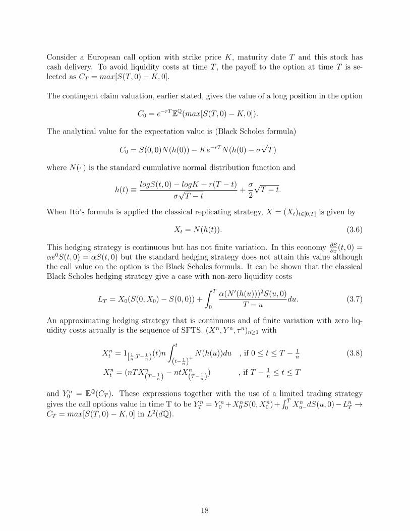
Consider a European call option with strike price K, maturity date T and this stock hascash delivery. To avoid liquidity costs at time T , the payoff to the option at time T is se-lected as CT = max[S(T, 0)−K, 0].
The contingent claim valuation, earlier stated, gives the value of a long position in the option
C0 = e−rTEQ(max[S(T, 0)−K, 0]).
The analytical value for the expectation value is (Black Scholes formula)
C0 = S(0, 0)N(h(0))−Ke−rTN(h(0)− σ√T )
where N(· ) is the standard cumulative normal distribution function and
h(t) ≡ logS(t, 0)− logK + r(T − t)σ√T − t
+σ
2
√T − t.
When Ito’s formula is applied the classical replicating strategy, X = (Xt)t∈[0,T ] is given by
Xt = N(h(t)). (3.6)
This hedging strategy is continuous but has not finite variation. In this economy ∂S∂x
(t, 0) =αe0S(t, 0) = αS(t, 0) but the standard hedging strategy does not attain this value althoughthe call value on the option is the Black Scholes formula. It can be shown that the classicalBlack Scholes hedging strategy give a case with non-zero liquidity costs
LT = X0(S(0, X0)− S(0, 0)) +
∫ T
0
α(N ′(h(u)))2S(u, 0)
T − udu. (3.7)
An approximating hedging strategy that is continuous and of finite variation with zero liq-uidity costs actually is the sequence of SFTS. (Xn, Y n, τn)n≥1 with
Xnt = 1[ 1
n,T− 1
n)(t)n
∫ t
(t− 1n)
+N(h(u))du , if 0 ≤ t ≤ T − 1
n(3.8)
Xnt = (nTXn
(T− 1n) − ntX
n
(T− 1n)) , if T − 1
n≤ t ≤ T
and Y n0 = EQ(CT ). These expressions together with the use of a limited trading strategy
gives the call options value in time T to be Y nT = Y n
0 +Xn0 S(0, Xn
0 )+∫ T
0Xnu−dS(u, 0)−LnT →
CT = max[S(T, 0)−K, 0] in L2(dQ).
18
4 Economies with Supply Curves for Derivatives
The extensions of the First and Second Fundamental Theorem hold in the economy describedin earlier chapters. If we use C2 smooth supply curve for the stock and allowing continuoustrading strategies there is a unique price for any option on the stock. This definition impliesthat the supply curve for trading an option is horizontal and therefore has no quantity im-pact on the price. If the supply curve is not horizontal arbitrage opportunities arises. Thedefinition is not consistent with reality and a model that analyzes liquidity risk should implysupply curves for both stocks and options.
The described supply curve does exist for stocks, but not for options in the example ofthe economy with liquidity risk, i.e. the previous chapter. This is because continuous tradingstrategies of finite variation enable the investor to avoid all liquidity costs in the stock. Liq-uidity costs still exist but they are non-binding and a modified classical theory still applies.Liquidity costs are binding in practice and to make them binding in theory either the C2
condition or continuous trading strategies must be removed. If continuous trading strategiesare removed the model consists with practice because these strategies are impossible to utilizeexcept as approximations thru simple trading strategies. But simple trading strategies havebinding liquidity costs.
4.1 Discrete Trading Strategies
Now the previous theory is modified to consider only discrete trading strategies defined asany simple SFTS. Xt where
Xt ∈ xτ01τ0 +N∑j=1
xτj1(τj−1,τj ]
τj are F stopping times for each j,xτj is in Fτj−1 for each predictable j
τ0 ≡ 0 and τj > τj−1 + δ for a fixed δ > 0.
These trading strategies are discontinuous because between every trade that is executed thereis a δ > 0 big time unit gap.
An arbitrage-free environment is obtained by this restriction of trading strategies. By intro-ducing the minimum distance δ between trades the market is not approximately complete. Inan incomplete (not approximately complete) market the cost of replicating an option dependson the chosen trading strategy. The second fundamental theorem fails which implies thatthere can be a quantity impact on the price of an option and the supply curve does not needto be horizontal.
There is some constraint on the supply curve due to no arbitrage and this can be stud-ied by the super-replication of options when using discrete trading strategies. The lower casevalues x and y denotes from now on discrete trading strategies. All discrete trading strategieshas the liquidity cost
LT =N∑j=0
[xτj+1
− xτj] [S(τj, xτj+1
− xτj)− S (τj, 0)
]. (4.1)
19

The hedging error for a discrete trading strategy with xT = 0 is
CT − YT = CT −
[y0 + x0S(0, 0) +
N−1∑j=0
xτj+1[S(τj+1, 0)− S(τj, 0)]
]+ LT .
There are two components to this hedging error, one of them is liquidity cost LT (equation4.1) and the other, the remainder of the previous expression, is the error in replicating theoptions payoff CT .
An upper bound on the price of a particular quantity of option is investigated. The costof a single call option on the stock is obtained as follows. Defined Zt = XtS(t, 0) + Yt as thetime t market-to-market value of the replicating portfolio. The optimization problem is
min(X,Y )
Z0 such that ZT ≥ CT = max(S(T, 0)−Ke−rT , 0) (4.2)
where
ZT = y0 + x0S(0, 0) +N−1∑j=0
xτj+1[S(τj+1, 0)− S(τj, 0)]− LT .
The solution to this problem requires a numerical approximation (see [CJPW] for a binomialapproximation to solve the problem). Liquidity costs in the underlying stock are quantitydependent. This gives that the cost of super-replication also is quantity dependent. An upperbound on the entire supply curve is created for the option by the cost of super-replicatinga number of shares of the option. There is a significant economically difference between theclassical price and the super-replication cost. [CJPW]
20

4.2 Transactional Costs
Transactional costs can be seen as liquidity risk where the hypothesis of the C2 supply curve isviolated. Three different types of transaction costs are discussed. All costs are per share unlessthere is another statement. Mathematics of the supply curve is used to study transactioncosts while ignoring liquidity issues. The supply curve is now known as the transaction curveand the goal is to see when continuous trading is possible. [C]
Definition 4.1 There are three kinds of transaction costs(1) Fixed transaction costs are per share stock price and defined by
S(t, x) = S(t, 0) +a
x.
(2) Proportionate transaction costs depend proportionately on the money value of the trade
S(t, x) = S(t, 0)(1 + βsign(x))
where β > 0 is the proportionate transaction cost per unit value.
(3) Combined fixed and proportionate transaction costs is defined different depending on the
(a) S(t, x) = S(t, 0) +β
x+ sign(x)γ1|x|>δ
where β, γ and δ are positive constants.
(b) S(t, x) = S(t, 0) +max(α, |x|c)
x
where α and c are positive constants.
This implies that when the transaction costs are fixed, only piecewise constant trading strate-gies are needed to do a model.
4.2.1 Fixed Transaction Costs
Fixed transaction costs when having continuous trading gives infinite costs at infinite time.The definition of fixed transaction costs together with trading strategy X =
∑n−1i=0 Xi1[Ti,Ti+1)
for trading times 0 = T0 ≤ T1 ≤ ... ≤ Tn = T gives the cumulative trading costs∑n−1
i=0 a1(Xi 6=Xi−1).If Xi 6= Xi−1 then this is equal to na. Now say that X has continuous paths the trading costsTC(X) with trading strategy X is
TC(X) = lim supn→∞
∑Tni ∈Πk
a1(XTni6=XTn
i+1) = lim sup
n→∞aNΠn(X)
where Πn is a finite increasing sequence of stopping times covering the interval [0, T ] and themesh of Πn tends to 0 as n→∞. NΠn(X) is the number of times that (Xi 6= Xi−1. For therandom stopping times of Πn lim supn→∞NΠn(X) =∞, unless X is almost certain piecewiseconstant. Continuous trading strategies have infinite transaction costs. If the trading strategyhas both jumps and continuous parts the transaction costs will also be infinite.
21
4.2.2 Proportional Transaction Costs
With proportional transactional costs there is possible to trade continuously if you use atrading strategy with paths with finite variation which is not possible with for example thestandard Black-Scholes hedge of a European call/put option. Proportional transaction costswith continuous trading are infinite if the trading strategy has paths of infinite variation. Astrategy X has paths of finite variation on [0, T ] for a subset Λ of Ω. The cumulative trans-
action costs are b∫ T
0S(u, 0)|dXu| almost surely on Λ where |dXu| denotes the total variation
(Stieltjes path by path integral) which are infinite on Λc. the constant b is the proportionatetransaction cost per unit value defined in definition 4.1, part 2.
If Πn is a sequence of random partitions tending to the identity on [0, T ] and X is a con-tinuous trading strategy, then the cumulative transaction costs for proportional costs can bewritten as
TC(X) = lim supn→∞
∑Tni ∈Πk
S(T nk , 0)|∆Xn,k|b
where ∆Xn,k = XnTk−Xn
Tk−1. When X has paths of finite variation this expression converges
to the path by path integral b∫ T
0S(u, 0)|dXu| (Stieltjes integral) and when X has paths of
infinite variation the expression diverges to ∞.
4.2.3 Combined Fixed and Proportional Transaction Costs
Combined fixed and proportional transaction costs with continuous trading create infinitecosts in finite time. If a trading strategy X has continuous paths then TC(X) denote thetransaction costs so that
TC(X) ≥ lim supn→∞
∑Tni ∈Πk
δ1(XTni6=XTn
i+1) = lim sup
n→∞δNΠn(X)
with some constant δ, Πn is as before a sequence of random partitions tending to the identityand NΠn(X) is the number of times XTn
i6= XTn
i +1 for the random stopping times of Πn. Thisleads to infinite costs.
4.3 Linear Supply Curves
The classical theory has unlimited liquidity and is embedded in the previously discussedstructure. The standard price process St = S(t, 0) can be deduced by reduce the supplycurve x → S(t, x) to x → S(t, 0). This is a line with slope 0 and vertical axis interceptS(t, 0). When the supply curve is linear it can be written on the form
x→ S(t, x) = Mtx+ bt (4.3)
where Mt = 0 if the classical theory should hold. Suppose this is taken as the null hypothesisBlais [Bl] has shown that this can be rejected at the 0.9999 significance level. From this theconclusion that the supply curve exists and is not trivial is derived.
By use linear regression it can be showed that the supply curve is linear for liquid stocks.
22

The slope and intercept is time varying and can be written as equation 4.3 where bt = S(t, 0)and (Mt)t≥0 is itself a stochastic process with continuous paths.
Theorem 4.2 A liquid stock with linear supply curve
x→ S(t, x) =: Mtx+ bt
and a cadlag (right continuous with left limits) trading strategy X with finite quadratic vari-ation has for a SFTS. the value in the money market account
Yt = −XtS(t, 0) +
∫ t
0
Xu−dS(u, 0)−∫ t
0
Mud[X,X]cu
The quadratic differential term can have jumps.
Non-liquid stocks raises a problem and the presented theory cannot hold in one particularpoint. The supply curve x → S(t, x) is not C2. Here the supply curve is jump linearand has one jump which can be described as the bid ask spread. The only place the C2
hypothesis is used is in the derivation of the SFTS. which makes it possible to eliminatethis hypothesis in the jump linear case. Because the supply curve is no longer continuousγ(t) = S(t, 0)− S(t, 0−) is defined as the bid ask spread where S(t, 0−) is the marginal askand S(t, 0) is the marginal bid. Now Λ = (u, ω) : ∆Xu(ω) and the supply curve has a jumplinear form like this
S(t, x) =
β(t)x+ S(t, 0) (x ≥ 0)α(t)x+ S(t, 0−) (x < 0)
(4.4)
Theorem 4.3 For an illiquid stock with a jump linear supply curve like the equation above(4.4) and a cadlag trading strategy X with finite quadratic variation the value in the moneymarket account for a SFTS. is
Yt = −XtS(t, 0) +
∫ t
0
Xu−dS(u, 0)−∫ t
0
β(u)1Λc(u) + α(u)1Λ(u)d[X,X]u −∫ t
0
1Λ(u)d[γ,X]u
where γ(t) = S(t, 0)− S(t, 0−) is the bid ask spread.
Let’s start with the money market process Y to show this. Y should satisfy
Yt = Y0 − limn→∞
∑k≥1
(∆Xn,k)S(T kn ,∆Xn,k) =
= X(0)S(0, X0)− limn→∞
∑k≥1
(∆Xn,k)[S(T kn ,∆Xn,k)− S(T kn , 0)
]− lim
n→∞
∑k≥1
(∆Xn,k)S(T kn , 0)
23
where ∆Xn,k = XTkn−XTk−1
n. From before we know that the last sum converges to−X0S(0, 0)−
XtS(t, 0) +∫ t
0Xu−dS(u, 0) and due to jump linear hypothesis the second sum∑
k≥1
(∆Xn,k)[S(T kn ,∆Xn,k)− S(T kn , 0)
]=
=∑k≥1
(∆Xn,k) 1(∆Xn,k≥0) [β(t)∆Xn,k + S(t, 0) + S(t, 0)] +∑k≥1
(∆Xn,k) 1(∆Xn,k<0) [α(t)∆Xn,k + S(t, 0−)− S(t, 0)]
=∑k≥1
(∆Xn,k)2 1(∆Xn,k≥0)β(t) +
∑k≥1
(∆Xn,k)2 1(∆Xn,k<0)α(t) + γ(t)∆Xn,k1(∆Xn,k<0)
where Λ = (u, ω) : ∆Xu(ω)<0. As the limit is applied, standard theorem from stochasticcalculus get the expression converges uniformly on compact time sets in probability to
−∫ t
0
β(u)1Λc(u) + α(u)1Λu)d[X,X]u −∫ t
0
1Λ(u)d[γ,X]u
This gives, compared to fixed transaction costs previously discussed, that bid ask spreadsnot necessarily generate infinite liquidity costs and due to this can use continuous tradingstrategies.
24

5 Method
Equation in Theorem 4.3 is used in the simulation. The second and third term is the actualliquidity costs. The first and second term is the calculated gain/loss and, in the end, theoption price, i.e. the value this relpicating portfolio has in the money account at time T withno money invested in the underlying asset. The option price, in a perfect economy withoutliquidity risk, is calculated using the analytic solutions of the choosen assets. This is definedin the next section.
Liquidity costs depends on the replicating portfolio adjustments X and the properties asupply curve. These properties are defined in the following sections. When all of this isdefined the simulation can be done. I have taken the liquidity risk and presented this aspercentage of the analytical price of the options which is the price a option would have in aperfect economy, i.e. a frictionless and competitive market.
5.1 Supply Curve
Liquid stock is defined in the sense that the order book is updated frequently and has manyentries. A two piece jump linear and linear supply curve is tested and gives a heuristic mea-sure of liquidity for a stock. In data set provided by Morgan Stanley less than 8 % wouldbe considered liquid by this criterion. Almost all stocks in this set are considered as illiquidstocks. [BP]
Because only 8 % of stocks in the US stock market can be considered liquid the supplycurve with jump linear form (equation (4.4)) is used in this simulation which represents illiq-uid stocks. This is the case with illiquid stocks and three parameters need to be defined tocreate the linear jump supply curve. Two slope parameters and one parameter which simu-lates the bid ask spread are created with this process. This involves a stochastic process andshould emulate a real supply curve. [BP]
A stochastic mean-reverting process (Ornstein-Uhlenbeck equation) is used to derive thejump linear supply curve. [O]
dXt = (m−Xt)dt+ σdWt
where Wt ∈ R is a Brownian motion and m is real.
The Ornstein-Uhlenbeck process is an example of a Gaussian process that has a boundedvariance and admits a stationary probability distribution. The difference between this pro-cess and a Brownian motion is in the drift term. The Brownian motion has a constant driftterm and the Ornstein-Uhlenbeck process has a drift term dependent on the current valueof the process. This gives that if the current value of the process is less than the long termmean, the drift will be positive and if the current value of the process is greater than the longterm mean, the drift will be negative. The mean acts as an equilibrium level for the process.
In this case m is the value which the mean-reverting process uses as the equilibrium. Threeprocesses are used to get samples of α, β and γ. α, β and γ are also used as m to evaluate
25
the stochastic supply curve with the expected value of m because these are set as the ex-pected value of the supply curve properties. σ in the mean-reverting process is the term thatdetermine the volatility and is defined as an arbitrary number with Xt ≥ 0 as a boundarycondition. This is done to ensure that the supply curve does not have a negative value, i.e.it is impossible to have a negative dependence between the underlying asset price and theorder size. Bt is a simple Brownian motion.
5.2 Derivatives
The derivatives which are used in this simulation are European, Digital and Asian options.Both put and call for each of the options are tested and all the options are of European style.
European options analytical solution for the price is derived from the Black Scholes pric-ing model [BS]. These solutions are used in comparing the liquidity cost and the price of theoptions.
ECt = StN(h1)−Ke−r(T−t)N(h2),
EPt = −StN(−h1) +Ke−r(T−t)N(−h2)
where St is the stock price, K is the strike price, r is the risk free rate, (T − t) is the time tomaturity and N(h) is the cumulative normal distribution of
h1 = ln(St/K) + (r + σ2/2)(T − t),h2 = h1 − σ
√T − t.
In this case Digital Cash-or-Noting options are used in the simulations. The closed formanalytical formula is given by [RR]
DCt = e−r(T−t)N(h2),
DPt = e−r(T−t)N(−h2).
The cash payout of this type of option is either 0 or 1 due to normalization. The price of thisoption can also be factorized with a predetermined cash amount.
The geometric averaging Asian options has closed analytical prices [KV]
AgCt = StN(g1)−Ke−r(T−t)N(g2),
AgPt = −StN(−g1) +Ke−r(T−t)N(−g2)
where
g1 = ln(St/K) + (b+ σ2g/2)(T − t),
g2 = g1 − σg√T − t,
σg = σ/√
3,
b = (r − σ2/6)/2.
26

There are no closed form solutions for arithmetic average Asian options. In this study ananalytical approximation is used. [TW]
AaCt = Ste(B−r(T−t)N(a1)−Kae
−r(T−t)N(a2),
AaPt = −Ste(B−r(T−t)N(−a1) +Kae−r(T−t)N(−a2)
where
a1 =[ln(St/Ka) + (B + σ2
a/2)(T − t)]/σa√
(T − t),a2 = a1 − σa
√T − t,
σa =√ln(M2/(T − t)− 2B),
B = ln(M1/(T − t)),
M1 =er(T−t) − 1
r(T − t),
M2 =2e(r+σ2)(T−t)
(r + σ2)(2r + σ2)(T − t)2+
2
r(T − t)2
(1
2r + σ2− er(T−t)
r + σ2
),
Ka =T
T − tK − t
T − tSavg,
and Savg is the average asset price.
5.3 Liquidity Costs
To derive the liquidity cost the classical replicating strategy, X need to be derived for eachof the options. This is easy to calculate using the analytical pricing formulas and in the casewith Asian options, the approximated analytical pricing formulas.
When X is derived the equation stated in Theorem 4.3 is used in the simulations. Theterms which adjust the value in the money market account to include liquidity risk is namedL1 and L2 where L1 depends on the slope of the supply curve and L2 depends on the bid askspread of the defined supply curve.
The liquidity cost L1 and L2 are discussed together and not separate. This gives a to-tal impact on the option price. This simulation is tested with 10 000 trajectories and 29
timesteps. Also the variance of these costs is derived. The model has also been stress testedto analyze the stability and also get some results in extreme cases.
A simple null hyphotesis test is done where liquidity costs = 0 are tested. The conclu-sion is that there definitely exist liquidity costs.
5.4 Empirical Liquidity Costs
A set of data is used from the Swedish stock Handelsbanken (SHB) to derive the real sup-ply curve. The complete order book for SHB is obtained with tick data from 2005-05-03 to2005-08-08 and are arbitrary chosen. This data set contains each posting of the top 5 bidsand the top 5 asks, including both prices and shares available. The top 5 bids and asks in
27

this data set are aggregated. This data shows how many shares the market is willing to buyor sell at prices near the quoted price as well as tick data for trades. Unlike standard tickdata, this gives information about supply and demand for a stock and also the actual pointson the supply curve.
This order book gives the numerical values of the supply curve which are taken as inputin the extended model and evaluated.
28

6 Result
To get liquidity costs in an option some input data need to be defined. The parts that needinput data in the model are the Black Scholes model and the supply curve. These data canbe selected to follow a specified stocks course but for now they are arbitrary decided.
6.1 Theoretical Supply Curve
The following simulations were done to show the size of the liquidity risk and also how dif-ferent input data influence liquidity costs.
The basic input data are chosen as:The spot price S0 = 100,The strike price K = 100,The risk free rate r = 0.05 (5%),The volatility σ = 0.30,The slope of the supply curve α = β = 10−4,The bid ask spread of the supply curve γ = 10−4.Time to maturity = 1 year,Timesteps = 256 (28).256 timesteps represent that the underlying asset is bought or sold 256 times in a year toreplicate all options.
Now the replicating strategy, X and the price of each option can be determined. Liquid-ity costs is presented as a percentage of the option price, analytically determined, to get agood view of the impact of liquidity costs on the option price and compare different types ofoptions.
29

Figure 2: This is the total liquidity risk in a European call option over time up to maturity,in this case 1 year with the basic data defined above.
Figure 2 is normalized with the option price at time T = 1. This price is not aggregated. Inthis figure it is clear that liquidity risk increases over time.
6.1.1 Liquidity Cost Sensitivity
This simulation is done with the basic data specified above. The liquidity cost is separatedin L1 and L2. L1 is the liquidity cost depending on the impact of the supply curve slope.L2 is the liquidity cost that the bid ask spread in the supply curve contributes to the totalliquidity cost L1+L2.
Liquidity cost L2 is in the order 102 larger than L1 and contributes with the largest partof the total liquidity cost of the European put and call option. The Digital option hasthe largest liquidity cost in percent of the option price. L2 in Asian options has a smallercontribution to the total liquidity cost compared to European and Digital options but thecontribution is still 101 larger than the contribution of L1. The liquidity cost is in the orderof 10−4 to 10−3 percent of the option price.
30

Liquidity costs L1 L2 L1+L2Percent of european C 6.831144e-006 1.229315e-004 0.000128Percent of european P 1.039274e-005 1.870250e-004 0.000195Percent of digital C 3.844734e-005 1.037360e-003 0.001060Percent of digital P 3.932158e-005 1.040257e-003 0.001071Percent of asiang C 1.053989e-005 3.282329e-004 0.000335Percent of asiang P 1.339956e-005 4.435834e-004 0.000452Percent of asiana C 9.743524e-006 1.549660e-004 0.000164Percent of asiana P 1.397039e-005 2.221923e-004 0.000235
Table 1: The liquidity cost are presented with L1 and L2, i.e. liquidity cost depending onthe supply curve slope and the bid ask spread.
6.1.2 Risk Free Rate Sensitivity
The basic data are used in this simulation but the risk free rate is changed. This is doneto analyze the sensitivity of this parameter in the model. The risk free rates are changed toextreme values to stresstest the model and get a ’worst case scenario’.
The liquidity risk changes by a factor of two when the risk free rate changes from zeroto five percent. Liquidity costs are bigger when the rate tends to zero. This simulation givesthe same differences in liquidity costs between different options, i.e. Digital options havehigher liquidity costs than other options. The non existing liquidity risk in arithmetic Asianoptions with rate zero depends on the approximate analytical solution. This solution doesnot work with risk free rate zero and also if the dividend is the same as the risk free rate[TW].
Liquidity costs r=0 r=5 r=10Percent of european C 0.000381 0.000128 0.000067Percent of european P 0.000381 0.000195 0.000155Percent of digital C 0.001072 0.001060 0.000525Percent of digital P 0.003942 0.001071 0.000400Percent of asiang C 0.000952 0.000335 0.000156Percent of asiang P 0.000860 0.000452 0.000324Percent of asiana C NaN 0.000164 0.000055Percent of asiana P NaN 0.000235 0.000113
Table 2: All the basic parameters are used except the risk free rate to show liquidity costs.
6.1.3 Volatility Sensitivity
In this simulation all basic parameters are used except the volatility parameter which changesto investigate the impact on liquidity costs. σ describes the volatility of the underlying assetused to price the options.
The extreme case of volatility does not change liquidity costs significant (table 2 in Ap-pendix). When σ is small liquidity costs decreases and when σ is large the liquidity risk
31

increases. This is related to the movement of the underlying asset. Larger movements in thestock leads to more adjustments in the replicating portfolio, hence larger liquidity costs.
6.1.4 Spot Price Sensitivity
To investigate the impact on liquidity costs depending on spot price of the underlying assetthe spot price are changed and also the strike price. The strike price follows the spot priceonly to ensure that all simulations, i.e. trajectories could be used in the simulation. If a biggap between spot price and strike price is enforced there would be too few trajectories thatcould give a satisfying result. If this scenario is interesting a number of different Monte Carlomethods could be used like importance sampling [G].
As before the option that has most liquidity costs is Digital options (table 4 in Appendix).It has about 101 larger liquidity costs than the other options. The spot prices 10, 100 and1000 are tested and the liquidity risk changes in the order of the spot prices. Spot price 100generates 10−1 smaller liquidity costs than spot price 10. This can be explained by the supplycurve. If you have to buy/sell the underlying asset due to the replicating portfolio a cheaperstock demands bigger orders to get the same value of an expensive stock.
6.1.5 Strike Price Relative Spot Price Sensitivity
This simulation is done with a gap between the spot price and the strike price. The gap is10 percent of the spot price. In this case all trajectories can be used to investigate liquiditycosts. If the gap would be large the same problem arises as above [G].
This gap sensitivity show an increase in liquidity costs when the strike price is 10 percentlarger than the spot price (table 5 in Appendix). This can be explained by the drive inthe underlying asset which depends on the risk free rate. The small liquidity risks in thecase when the spot price is 10 percent larger than the strike price are quite easy to intuitiveunderstand. If there is almost no risk that the price drops under the strike price, there is noneed to adjust the replicating portfolio as much as with the case when the strike price andthe spot price are almost equal.
6.1.6 Supply Curve Slope Sensitivity
In this simulation the supply curve slope are changed but all the other input data are set asthe basic data. The supply curve has two slope parameters but they are put as the same.This is only used when specified stocks are used and is not relevant in this specific simulation.The slopes used are 10−2, 10−4 and 10−6. 10−2 is an extreme case and illustrates a stock withvery high liquidity risk. This does not regard stocks with high turnover, but in a financialcrisis the supply curve has a steep slope.
As expected, liquidity costs increases when the curve has a steep slope (table 6 in Appendix).The change from 10−4 to 10−2 has about a 101 percent impact to liquidity costs. The digitaloptions have still the largest liquidity risk.
32

6.1.7 Supply Curve Bid Ask Spread Sensitivity
The bid ask spread of the supply curve are changed in this simulation but all other inputshave the basic inputs. The bid ask spread is the spread between the highest bid and thelowest ask price.
The bid ask spread has a larger impact on liquidity costs on all options than the supplycurve slope (table 7 in Appendix). When the bid ask spread is 10−2 the liquidity risk is in theorder of 10−1 percent in Digital options and 10−2 percent in the other options. The changein liquidity costs is of a ratio of one-to-one, a change in the bid ask spread of 101 makes animpact of 101 percent on liquidity costs.
6.1.8 Timestep Sensitivity
To investigate the impact of the frequency of adjusting the replicating portfolio the timestepinput is changed. 256 timesteps are used in the basic data and can be described as adjustingthe portfolio one time a day when the option expires after one year.
The impact of adjusting the replicating portfolio 64 times and 1024 times is not large onliquidity costs (table 8 in Appendix). It also decreases as the timesteps tends to infinity.Digital options have still a higher liquidity risk.
6.1.9 Time to Maturity Sensitivity
This simulation investigates the impact of the options lifespan. A half year, a year and twoyears are used as input data. All other parameters are set as the basic data defined above.
Liquidity costs depending on time to maturity does not change drastically (table 9 in Ap-pendix).When the lifespan is changed from two years to a half year liquidity costs gets about50 percent larger. The Digital options doubles in liquidity costs in this case. Digital optionsare more sensitive and liquidity in this case more than doubles.
6.1.10 Worst Case Scenario
A simulation is made, not with the basic data but with the worst thinkable cases in everyparameter in a liquidity cost perspective. This is done to illustrate a ’worst case scenario’.The model can be used to simulate these scenarios but it is important to realize that theinput data in the model is as significant as the result.
33

Liquidity costs Worst casePercent of european C 0.399261Percent of european P 0.246262Percent of digital C 1.229960Percent of digital P 0.791695Percent of asiang C 0.916483Percent of asiang P 0.338761Percent of asiana C NaNPercent of asiana P NaN
Table 3: This simulations input data is S0 = 10, K = 11, r = 0, σ = 0.50 α = β = 10−2,γ = 10−2, Time to maturity = 1 year and timesteps = 64.
The parameter with the largest impact on liquidity costs is the bid ask spread. The liquidityrisk is an add-on to the option. The analytic approximation of the arithmetic Asian optionsare not possible to calculate with r=0. Liquidity costs of these options should be a bit lowerthan for the geometric Asian options as the have throughout these results.
6.2 Empirical Supply Curve
The stock Handelsbanken AB has been used as a guideline of the real economy and has theproperties α = 1.2 ∗ 10−7, β = 1.4 ∗ 10−6 and γ = 2.9 ∗ 10−3. This is a stock with significantmovement in shares which gives an upper bound in the property parameters. The parametersin the Black Scholes model are defined as the basic parameters defined before but with thespot price 165. This is done to emulate the stock to some extent.
Liquidity costs SHB L1 L2 L1+L2Percent of european C 5.222830e-008 0.002117 0.002121Percent of european P 7.945890e-008 0.003220 0.003227Percent of digital C 8.029939e-008 0.017954 0.018022Percent of digital P 1.438868e-007 0.017821 0.017767Percent of asiang C 7.406151e-008 0.005651 0.005660Percent of asiang P 9.315360e-008 0.007639 0.007651Percent of asiana C 7.116521e-008 0.002662 0.002664Percent of asiana P 1.020376e-007 0.003817 0.003819
Table 4: This simulation presents the liquidity risk in an option with HSB as the underlyingasset.
In this case the liquidity cost L2, which depend on the bid ask spread is the factor thatcontributes with almost all liquidity cost.
34

7 Conclusions
7.1 Theory
This paper extends the classical arbitrage pricing theory to include liquidity risk. This is ac-complished by study the underlying asset price depending on the trading size. The first andsecond fundamental theorems is extended and proved to hold. The economy is showed to bearbitrage free, like the first theorem, if the stochastic process for the price for a marginal tradehas an equivalent martingale probability measure. The second theory also approximatelyholds. If the martingale measure is unique the markets will be approximately complete.
In an approximately complete market the derivative prices is equal to the classical arbitragefree price of the derivative security. This is a horizontal linear supply curve. To attain anupward sloping curve one solution is to preclude continuous trading strategies. This impliesan incomplete market and minimal cost super-replicating trading strategies are discussed inthis regard. A model is derived in the liquid and illiquid stock case and definitions are maderegarding liquidity and illiquidity to attain a sound theoretical solution.
When a classical option price approach is done and no softening of the price is made, i.e. noimpact on the price due to order size, the literature supports three general conclusions [J]. Thefirst is that the classical option price is true on average even when liquidity risk is included.The second conclusion is that although the classical (theoretical) option hedge cannot beapplied as theory prescribes, the discrete approximations often provide reasonable approxi-mations [JT]. These discrete approximations are also consistent with upward sloping supplycurves. The third conclusion is that risk management measures like Value-at-Risk (VaR) arebiased low due to the exclusion of liquidity risk, but simple adjustments for liquidity risk torisk measures like VaR are available.
7.2 Result
Results in the theory are used in deriving a theoretical sound model that takes liquidity costsin to consideration. This model has been tested in theory and practice.
The largest contribution to liquidity costs is the bid ask spread γ on the supply curve.Liquidity costs with the basic data used are in the order 10−4 percent of the option priceexcept for the Digital option with 10−3 percent of the option price. This is not a significantimpact on the price. Only at large turnovers this could generate large costs.
The Digital options have a larger liquidity costs than all the other options because the repli-cating portfolio in this case has to be adjusted more frequently.
The arithmetic Asian options have a smaller impact on liquidity costs compared to the geo-metric Asian options. The geometric option does not exist and is only used to approximatethe value or costs to the real arithmetic Asian option. The geometric option is in pricingmodels underpriced compared to the real arithmetic Asian option and this also affects theliquidity cost [KV]. The analytic approximation of the arithmetic Asian option cannot bedefined when the risk free rate is zero but the geometric closed solution can which gives a
35

good approximation of liquidity costs.
The worst case scenario had liquidity costs as big as one percent. This does not seem largebut if the financial institutions supporting the option market only take a commission of 0.1to 1 percent this profit disappear.
Options using the stock HSB as the underlying asset has a liquidity risk in the order of10−2 percent of the option prices. This is calculated with a stock that has a large turnovercompared to other stocks in the Swedish stock market but it is still defined as an illiquidstock because of a real bid ask spread over the collected book data used.
Swedens stock market is small compared to the market in USA and almost all stocks inthat market are considered illiquid with my definition. It is not strange that almost all stocksin the Swedish stock market are considered illiquid. A smaller market contributes with largerliquidity costs in options.
The liquidity is in this theory an add on and aggregates over time with linear properties(figure 2). The slope of the liquidity risk gets steeper in a financial crisis when the market isilliquid.
An interesting area to research further is liquidity costs in an economy in crisis, when thesupply curve has a steep slope. This model of liquidity costs is a good tool in risk manage-ment and gives a good estimation of worst case scenario. Also exact liquidity costs can becalculated using the actions of the broker as input.
When brokers act perfect from a modeling perspective, they can arbitrarily approximate aperfect hedging strategy with continuous strategies with paths of finite variation. In practicecontinuous trading, both financially and physically are impossible, all trading is of necessitydiscrete. Despite of this the result shows that one can get arbitrarily small liquidity chargesby trading with high frequency in small amounts. If the attention is directed to not only oneoption, but instead a portfolio of several options, liquidity issues do arise in an importantway, using this model with linear supply curves. Liquidity risk cannot be hedged, it is abinding cost.
To investigate the sensitivity of the input in the extended theory would be interesting toresearch further. This is not only interesting when modeling a fictitious economy in a crisis,but also how different input affect how the brokers should act.
It would be interesting to test this model on a real financial institution and see the im-pact of this liquidity risk in actual money. The turnover in the option market supported bya large financial institute is substantial and a small percent in liquidity costs could be a largeamount of money and the option price may need to be adjusted.
36

8 References
[B] T. Bjork, Arbitrage Theory in Continuous Time, Second Edition, MPG Books Group,Oxford, New York. 2004.
[Bl] M. Blais, Liquidity and Data,Ph.D. thesis, Cornell University. 2005.
[BP] M. Blais and P. Protter, An Analysis of the Supply Curve for Liquidity Risk throughBook Data, in preparation. 2010.
[BS] F. Black and M. Scholes, The Pricing of Options & Corporate Liabilities, Journal ofPolitical Economy. May/June, Vol 81, no 3, p.637. 1973.
[C] U. Cetin, Default and Liquidity Risk Modeling, Ph.D. thesis, Cornell University. 2003.
[CJP] U. Cetin, R. Jarrow and P. Protter, Liquidity Risk and Arbitrage Pricing Theory,Finance and Stochastics, 8, p.311-341. 2004.
[CJPW] U. Cetin, R. Jarrow, P. Protter and M. Warachka, Pricing Options in an ExtendedBlack Scholes Economy with Illiquidity: Theory and Empirical Evidence, working paper,Cornell University. 2004.
[CM] J. Cvitanic and J. Ma, Heding Options for Large Investor and Forward-BackwardSDEs,Annals of Applied Probability, 6, p.370-398. 1996.
[G] P. Glasserman, Monte Carlo Methods in Financial Engineering, Springer, USA. 2004.
[GM] S.J. Grossman and M.H. Miller, Liquidity Risk and Option Pricing Theory,Journal ofFinance, 43, p.617-633. 1988.
[H] J. C. Hull, Options, Futures, and other Derivatives, Seventh Edition, Pearson PrenticeHall, Upper Saddle River, New Jersey. 2009.
[HP] J.M. Harrison and S. Pliska, Martingales and Stochastic Integrals in the Theory ofContinuous Trading, Journal of Finance, 43, p.617-633. 1981.
[J] R.A. Jarrow, Liquidity Risk and Classical Option Pricing Theory, 2005. In book: L. Matzand P. Neu, Liquidity Risk Mannagement, Wiley and Sons, Singapore, Asia, p.360-376.2007.
[JP] R.A. Jarrow and P. Protter, Liquidity Risk and Option Pricing Theory, Handbook inOperation Research and Management Science: Financial Engineering, J. Birge and V.Linetsky, eds., North Holland, p.727-762. 2007.
[JT] R. Jarrow and S. Turnbull, Derivative Securities, South-Western, Division of ThomsonLearning, USA. 2000.
[K] A. Kyle, Continuous Auctions and Insider Trading, Econometrica, 53, p.1315-1335.1985.
[KV] A.G.Z. Kemna and A.C.F. Vorst, A Pricing Method for Options Based on AverageAsset Values,Journal of Banking and Finance, 14, p.113-129. 1990.
37

[O] B. Øksendal, Stochastic Differential Equations, Sixth Edition, Springer, Heidelberg,Berlin. 2007.
[P] L. H. Pedersen, Liquidity Risk and the Current Crisis, The First Global Financial Crisisof the 21st Century, Part 2, A VoxEU.org Publication p.147-152. 2008.
[RR] E. Reiner and M. Rubstein, Unscrambling the Binary Code, Risk, 4, October. 1991.
[TW] S.M. Turnbull and L.M. Wakeman, A Quick Algorithm for Pricing European AverageOptions, Journal of Financial and Quantitative Analysis, Vol 26, no 3, September,p.377-389. 1991.
38

Appendix
Volatility Sensitivity
Liquidity costs sigma=0.1 sigma=0.3 sigma=0.5Percent of european C 0.000106 0.000128 0.000117Percent of european P 0.000372 0.000195 0.000150Percent of digital C 0.000926 0.001060 0.000775Percent of digital P 0.000803 0.001071 0.001240Percent of asiang C 0.000235 0.000335 0.000307Percent of asiang P 0.000719 0.000452 0.000335Percent of asiana C 0.000072 0.000164 0.000187Percent of asiana P 0.000215 0.000235 0.000232
Table 5: The basic data are used except for the volatility which is changed.
Spot Price Sensitivity
Liquidity costs s0=10, K=10 s0=100, K=100 s0=1000, K=1000Percent of european C 0.001285 0.000128 0.000013Percent of european P 0.001955 0.000195 0.000020Percent of digital C 0.014222 0.001060 0.000104Percent of digital P 0.014298 0.001071 0.000105Percent of asiang C 0.003355 0.000335 0.000034Percent of asiang P 0.004526 0.000452 0.000046Percent of asiana C 0.001645 0.000164 0.000016Percent of asiana P 0.002358 0.000235 0.000024
Table 6: The basic data are used except for the spot price and the strike price which arechanged but has the same value.
Strike Price Relative Spot Price Sensitivity
Liquidity costs s0=100, K=90 s0=100, K=100 s0=100, K=110Percent of european C 0.000035 0.000128 0.000651Percent of european P 0.000131 0.000195 0.000445Percent of digital C 0.000336 0.001060 0.001406Percent of digital P 0.000259 0.001071 0.000950Percent of asiang C 0.000052 0.000335 0.001676Percent of asiang P 0.000349 0.000452 0.000557Percent of asiana C 0.000008 0.000164 0.001084Percent of asiana P 0.000051 0.000235 0.000394
Table 7: The basic data are used except for the spot/strike price gap which is changed.
1

Supply Curve Slope Sensitivity
Liquidity costs α = β = 10−2 α = β = 10−4 α = β = 10−6
Percent of european C 0.000808 0.000128 0.000122Percent of european P 0.001229 0.000195 0.000185Percent of digital C 0.005020 0.001060 0.001029Percent of digital P 0.005145 0.001071 0.001022Percent of asiang C 0.001391 0.000335 0.000325Percent of asiang P 0.001795 0.000452 0.000439Percent of asiana C 0.001142 0.000164 0.000153Percent of asiana P 0.001638 0.000235 0.000220
Table 8: The basic data are used except for the supply curve slope which is changed.
Supply Curve Bid Ask Spread Sensitivity
Liquidity costs γ = 10−2 γ = 10−4 γ = 10−6
Percent of european C 0.012200 0.000128 0.000008Percent of european P 0.018561 0.000195 0.000012Percent of digital C 0.103018 0.001060 0.000049Percent of digital P 0.102616 0.001071 0.000049Percent of asiang C 0.032564 0.000335 0.000014Percent of asiang P 0.044011 0.000452 0.000018Percent of asiana C 0.015377 0.000164 0.000011Percent of asiana P 0.022047 0.000235 0.000016
Table 9: The basic data are used except for the bid ask spread of the supply curve which ischanged.
Timestep Sensitivity
Liquidity costs 1024 timesteps 256 timesteps 64 timestepsPercent of european C 0.000120 0.000128 0.000175Percent of european P 0.000182 0.000195 0.000266Percent of digital C 0.001049 0.001060 0.000945Percent of digital P 0.000814 0.001071 0.001666Percent of asiang C 0.000317 0.000335 0.000436Percent of asiang P 0.000428 0.000452 0.000582Percent of asiana C 0.000137 0.000164 0.000290Percent of asiana P 0.000196 0.000235 0.000416
Table 10: The basic data are used except for the timesteps which is changed.
2

Time to Maturity Sensitivity
Liquidity costs 0.5 year 1 year 2 yearsPercent of european C 0.000162 0.000128 0.000107Percent of european P 0.000218 0.000195 0.000195Percent of digital C 0.001237 0.001060 0.000632Percent of digital P 0.002467 0.001071 0.000468Percent of asiang C 0.000406 0.000335 0.000285Percent of asiang P 0.000500 0.000452 0.000439Percent of asiana C 0.000255 0.000164 0.000119Percent of asiana P 0.000330 0.000235 0.000198
Table 11: The basic data are used except for the lifespan of the options which is changed.
3