option pricing for discrete hedging and non-gaussian processes pricin… · both methods were...

Option Pricing forDiscrete Hedging and

Non-Gaussian Processes

�Kellogg College

University of Oxford

A thesis submitted in partial fulfillment of the requirements forthe MSc in

Mathematical Finance

November 24, 2002

Uwe Kupferschmied

d-fine

Option Pricing for Discrete Hedging and

Non-Gaussian Processes

Kellogg CollegeUniversity of Oxford

A thesis submitted in partial fulfillment of the requirements forthe MSc in

Mathematical Finance

November 24, 2002

The Black-Scholes option pricing method is correct under certain assumptions, among

others continuous hedging and a log-normal underlying process. If any of these two

assumptions is not fulfilled, a risk-less replication of an option is in general not possi-

ble. To handle this case, a pricing method was proposed by Bouchaud and Sornette.

Similar to Black-Scholes, a hedging portfolio is considered. The hedging strategy is

such that the risk of the hedging portfolio is minimized. An option price is then

deduced from this hedging strategy. Since a risk remains, the price includes a risk

premium.

In this thesis, a new alternative method is presented, which instead of minimizing

the portfolio risk minimizes the option price. This makes the option most competitive

on the market. For the option writer, the ratio of return to risk is, by definition of

the method, the same as for the Bouchaud-Sornette approach.

Both methods were compared with each other. For typical options, differences of

up to 10 % of the price were found. The risk premium as well as fat tails in the

underlying process give rise to volatility smiles for both methods. Furthermore, it

was found that both methods are consistent with Black-Scholes pricing. The results

converge towards the Black-Scholes result in the continuous time limit for a log-normal

process.

Contents

1 Introduction 1

2 Basic Concepts 3

2.1 Asset Price Model . . . . . . . . . . . . . . . . . . . . . . . . . . . . . 3

2.1.1 Statistical Variable for the Price Process . . . . . . . . . . . . 3

2.1.2 Probability Density of the Process . . . . . . . . . . . . . . . . 4

2.1.2.1 Stable Distributions . . . . . . . . . . . . . . . . . . 4

2.1.2.2 Real Price Dynamics . . . . . . . . . . . . . . . . . . 6

2.2 The Hedging Portfolio . . . . . . . . . . . . . . . . . . . . . . . . . . 6

2.2.1 Self-Financing Trading Strategies . . . . . . . . . . . . . . . . 6

2.2.2 The Value of the Hedging Portfolio . . . . . . . . . . . . . . . 9

2.2.3 The Moments of the Portfolio Value . . . . . . . . . . . . . . . 10

3 Option Pricing Methods 11

3.1 Overview . . . . . . . . . . . . . . . . . . . . . . . . . . . . . . . . . . 11

3.2 The Option Price Equation . . . . . . . . . . . . . . . . . . . . . . . 12

3.3 The Bouchaud-Sornette Approach . . . . . . . . . . . . . . . . . . . . 13

3.3.1 The Optimal Hedging Strategy . . . . . . . . . . . . . . . . . 13

3.3.2 Options in a Risk Neutral World . . . . . . . . . . . . . . . . 14

3.4 The Minimal Price Approach . . . . . . . . . . . . . . . . . . . . . . 15

3.4.1 Overview . . . . . . . . . . . . . . . . . . . . . . . . . . . . . 15

3.4.2 The Optimal Hedging Strategy . . . . . . . . . . . . . . . . . 16

3.4.2.1 Zero Price of Risk . . . . . . . . . . . . . . . . . . . 16

3.4.2.2 Non-Zero Price of Risk . . . . . . . . . . . . . . . . . 16

3.5 The Continuous Time Limit . . . . . . . . . . . . . . . . . . . . . . . 17

i

4 Comparison of Pricing Methods 20

4.1 Introduction . . . . . . . . . . . . . . . . . . . . . . . . . . . . . . . . 20

4.2 Asset Processes and Options . . . . . . . . . . . . . . . . . . . . . . . 21

4.2.1 The Underlying Process . . . . . . . . . . . . . . . . . . . . . 21

4.2.1.1 Log-Normal Process . . . . . . . . . . . . . . . . . . 21

4.2.1.2 Fat Tail Process . . . . . . . . . . . . . . . . . . . . 22

4.2.2 Option Characteristics . . . . . . . . . . . . . . . . . . . . . . 24

4.3 Software Implementation . . . . . . . . . . . . . . . . . . . . . . . . . 24

4.3.1 Price and Strategy Calculation . . . . . . . . . . . . . . . . . 24

4.3.1.1 Solution Algorithm . . . . . . . . . . . . . . . . . . . 24

4.3.1.2 Calculation of Expectation Values . . . . . . . . . . 25

4.3.1.3 Calculation of Probabilities . . . . . . . . . . . . . . 26

4.3.2 Monte Carlo Simulation . . . . . . . . . . . . . . . . . . . . . 27

4.3.3 Error Estimate . . . . . . . . . . . . . . . . . . . . . . . . . . 28

4.3.4 Hardware and Performance . . . . . . . . . . . . . . . . . . . 30

4.4 Results . . . . . . . . . . . . . . . . . . . . . . . . . . . . . . . . . . . 30

4.4.1 Dependence on the Rehedging Frequency . . . . . . . . . . . . 30

4.4.2 Comparison of Hedging Strategies . . . . . . . . . . . . . . . . 35

4.4.3 Dependence on the Price of Risk . . . . . . . . . . . . . . . . 39

4.4.4 Implied Volatility Matrix . . . . . . . . . . . . . . . . . . . . . 40

4.4.4.1 Plain Vanilla Options . . . . . . . . . . . . . . . . . 40

4.4.4.2 Binary Options . . . . . . . . . . . . . . . . . . . . . 45

4.4.5 Drift Dependence . . . . . . . . . . . . . . . . . . . . . . . . . 48

5 Conclusions 52

A Formulas for Expectation Values 55

A.1 Strategy Independent Integrals . . . . . . . . . . . . . . . . . . . . . 55

A.2 Strategy Dependent Integrals . . . . . . . . . . . . . . . . . . . . . . 56

B Continuous Time Limit 59

B.1 The Limit for Expectation Values . . . . . . . . . . . . . . . . . . . . 59

B.2 The Limit for the Hedging Strategy . . . . . . . . . . . . . . . . . . . 62

Bibliography 63

ii

List of Figures

2.1 Log-return distribution for IBM stocks. . . . . . . . . . . . . . . . . . 7

4.1 Probability distributions for the fat tail asset process. . . . . . . . . . 23

4.2 Plain vanilla call premium as a function of the rehedging frequency. . 32

4.3 Risk and risk premium as a function of the rehedging frequency. . . . 33

4.4 Profit distributions. . . . . . . . . . . . . . . . . . . . . . . . . . . . . 34

4.5 Plain vanilla option premium as a function of the rehedging frequency. 36

4.6 Binary option premium as a function of the rehedging frequency. . . . 37

4.7 Comparison of hedging strategies. . . . . . . . . . . . . . . . . . . . . 38

4.8 Option premium as a function of the price of risk. . . . . . . . . . . . 39

4.9 Implied volatility matrix for a plain vanilla call. . . . . . . . . . . . . 40

4.10 Volatility smiles for different hedging strategies. . . . . . . . . . . . . 41

4.11 Volatility smiles for different rehedging frequencies. . . . . . . . . . . 42

4.12 Volatility smiles for asymmetric probability distributions. . . . . . . . 43

4.13 Term structures of implied volatilities. . . . . . . . . . . . . . . . . . 44

4.14 Volatility smiles at different maturities for a log-normal process. . . . 46

4.15 Volatility smiles at different maturities for the fat tail process. . . . . 47

4.16 Implied volatility matrix for a binary call. . . . . . . . . . . . . . . . 48

4.17 Black-Scholes price of a binary call as a function of strike and volatility. 49

4.18 Implied volatility as a function of the strike for a binary call. . . . . . 50

4.19 Unexpected profit as a function of the real asset drift. . . . . . . . . . 51

iii

Chapter 1

Introduction

A milestone in the development of derivative pricing was the discovery by Black

and Scholes in 1973 that under certain assumptions options can be replicated by an

investment in the underlying and a cash balance[1]. In an arbitrage free economy, the

price of the derivative is then directly given by the value of the replicating portfolio.

Since then, a whole pricing theory was build on the replication method. The unique

price from this valuation is called the fair price.

To get a unique price, amongst others, the following conditions must hold [2, 3, 4]:

• Either trading can be done continuously in time or the underlying process fol-

lows a binominal model. In a binominal model, only two states for the underly-

ing price change exist for each time step. In this case, the risk can be eliminated

completely even for discrete hedging. In a trinominal model with three possible

price changes per time step, a risk remains.

• The process of the underlying has to be known for infinitesimal time steps. It

has to be a semi-martingale. In the standard Black-Scholes model, a log-normal

process is assumed.

Obviously, these conditions are not fulfilled in the real word. Hedging can only

take place in discrete time steps. And the binomial model is not sufficient to describe

the underlying price movements because of fat tails in the price distributions. Fat tails

cannot be reproduced with the binominal model since the binominal model converges

towards a Gaussian probability distribution for infinitesimal small time steps.

Another problem comes from the fact, that continuous hedging requires the un-

derlying process to be known for infinitesimal time steps. This information cannot

be extracted directly from market data where one has access only to price changes

for finite time intervals. So, one has to find a process which is a semi-martingale and

1

which fits to market data. It is not guaranteed that such a process always exist. If it

does exist, the process might not have been studied in the literature yet, so that the

valuation is not trivial.

This thesis studies the case where hedging is not continuous. This is a more

realistic assumption than continuous hedging and also makes it easy to model the

underlying process. Since only discrete time intervals are considered, the underlying

price change has to be known only for these time steps and therefore can be directly

taken from market data. This removes restrictions on the underlying process and

makes it easy to include special features of the underlying process, like fat tails.

For such a case, Bouchaud and Sornette proposed an approach to option pricing

in 1994 [5, 6]. It is based on the Black-Scholes idea to build up a replication portfolio.

The replication should be as perfect as possible. In the sense of Bouchaud and

Sornette, this means that the hedging strategy minimizes the risk of the hedging

portfolio. The fair option price is then given by the replication strategy. Since a risk

remains, a risk premium has to be added to the fair price.

The shortcoming of the Bouchaud-Sornette method is that there is no argument

why their option price should be accepted by the market. In the Black Scholes world,

there is the no-arbitrage argument which guarantees that the price of the replicated

derivative is the market price. Such an argument is missing for the Bouchaud-Sornette

approach.

In this thesis another, new method is presented. As the other methods, it is based

on a hedging portfolio for which an optimal hedging strategy has to be found. By

definition of the method, it will give the same ratio of return to risk as the Bouchaud-

Sornette approach. But instead of minimizing the risk, the option writer minimizes

the option price. This makes the option most competitive on the market and provides

the argument why this price should be the market price. This argument, of course,

only holds as long as all investors have the same risk preference. In general, a model-

independent, unique price doesn’t exist whenever a risk remains for the option writer.

2

Chapter 2

Basic Concepts

2.1 Asset Price Model

The most basic input to a derivative pricing method is the description of the under-

lying. Describing the underlying means to have a model for the statistical movement

of the underlying price S(t) with time. Such models will be discussed in this sec-

tion. Since this thesis has its focus on comparing pricing models, only assets will be

considered as underlying, which is the simplest case.

2.1.1 Statistical Variable for the Price Process

The very first thing in working out a statistical asset price model is to decide which

statistical variable to use. There are two obvious choices, namely absolute price

differences

∆Si = S(ti)− S(ti−1) (2.1)

with ti = ti−1 + ∆t or price returns

Ri =S(ti)

S(ti−1)(2.2)

which are relative changes. The reason why to think about the choice of variables

is to simplify the model. A simple model would be based on independent identically

distributed (i.i.d.) random variables. A time series of independent random variables xi

has the property that the correlation between the variables at different times vanish

E[xi, xj] = δij E[x2i ] (2.3)

Here, E[. . .] stands for the expectation value. The variables are identically distributed

if the moments E[xni ] are independent on time, so the moments are equal for any i.

3

Studies on data show that for short time steps absolute changes are closer to an

i.i.d. variable, while for longer times (about one month on liquid markets) this is the

case for returns [7]. In this thesis, returns will be chosen although the time scale

given by the rehedging frequency of options is smaller than a month. But this choice

allows to compare with the standard Black-Scholes model for a log-normal process.

To be precise, the logarithm, log Ri, of the return will be used instead of the return

itself, so that the variable is additive:

log Rtj ,tk ≡ logS(tk)

S(tj)=

k∑i=j+1

logS(ti)

S(ti−1)=

k∑i=j+1

log Ri (2.4)

It is more convenient to work with an additive random variable and the logarithm

restricts the asset price to positive values.

Another question is which time scale to use. In equations 2.1 and 2.2, the argument

ti should be understood as the trading time in days with equidistant time intervals.

Instead, one could also think about using the real time, including weekends, or to

use the number of transactions as a time measure [8]. Using the trading time is the

standard choice for asset models.

Apart from choosing the random variable and the time scale, a probability density

to describe the distribution of the values of the random variable will complete the

model. The probability density will be addressed in the next section.

2.1.2 Probability Density of the Process

2.1.2.1 Stable Distributions

Suppose there is an additive i.i.d. random variable xi, for which the probability density

p(x) is given. If xi describes a price change then it is of interest how the overall price

change

Xn = x1 + x2 + · · ·+ xn (2.5)

for several time steps is distributed. The probability distribution pn(X) for the sum

is obtained by the nth autoconvolution of p(x). The autoconvolution can be easily

done by applying a Fourier transformation to the probability density

φ(q) =

∫ ∞

−∞p(x) eiqx dx (2.6)

A convolution corresponds to a multiplication in Fourier space. Therefore, the Fourier

transformation of pn(X) is

φn(q) = [φ(q)]n (2.7)

4

and the inverse transformation yields

pn(X) =1

2π

∫ ∞

−∞[φ(x)]n e−iqx dq (2.8)

The question of what happens if n goes to infinity is subject to a central limit

theorem. For any probability density p(x) with tails p(x → ±∞) ∝ c±/ |x|1+α and

0 < α ≤ 2, the function log φn(q) will converge towards a member of a class of

functions [9]

log φ(q) =

iµq − γ|q|α

[1− iβ q

|q| tan(

π2α)]

α 6= 1

iµq − γ|q|[1 + iβ q

|q|2π

ln |q|]

α = 1

(2.9)

with 0 < α ≤ 2, γ ≥ 0, µ any real number, and −1 ≤ β ≤ 1. This class of functions

describes Levy processes which have the following characteristics [8]

• The process is stable.

A stable function has the same functional form after convolution. Examples are

the Gaussian and Lorentzian distributions.

• For α = 2 the process is a Gaussian and for α = 1, β = 0 a Lorentzian process.

Apart from these processes, only for α = 0.5, β = 1 (Levy-Smirnov) the analytic

form of the probability distribution is known.

• The probability distribution has power law tails for α 6= 2:

p(x) ∝ 1

|x|1+αfor large |x| (2.10)

• The variance is infinite for α 6= 2. Only the Gaussian has finite variance.

• Levy functions are the only attractors for probability functions pn(X) in the

limit n →∞.

From the statements above, we can conclude that in continuous time any price

process of i.i.d. random variables with tails p(x → ±∞) ∝ c±/ |x|1+α and 0 < α ≤ 2

will result in a Levy distribution for finite time intervals. If the variance of a process

is finite, it will converge towards a Gaussian process. In this case, the variance of Xn

will scale like n, e.g. for n = 2

Var[X2] = E[(x1 + x2 − E[x1 + x2])

2] (2.11)

= 2 · E[x2]+ 2 · E [x1 · x2]− 2 · E [(x1 + x2) · E[x1 + x2] ] + 4 · E[x]2

= 2 · E[x2]+ 2 · E [x]2 − 8 · E [x]2 + 4 · E[x]2

= 2 · E[x2]− 2 · E [x]2 = 2 · Var[x]

5

If each xi is a price change for one equidistant time step ∆t, the variance scales with

∆t.

2.1.2.2 Real Price Dynamics

In the literature, sophisticated analysis of price changes can be found [7, 8, 10]. The

main results are illustrated by Figure 2.1 where daily log-returns of the IBM stock

are shown:

• A Gaussian distribution fails to describe the fat tails in data.

• The variance is finite.

• It is not a Levy distribution since the variance is finite and the distribution

doesn’t follow a Gaussian.

From these observations on data and the statements from the last section, we can

conclude that in continuous time price changes cannot be described by i.i.d. random

variables. However, if we give up to work in continuous time, the assumption of i.i.d.

random variables is reasonable, e.g. the return for two days is quite well described

by a convolution of twice the daily return distribution.

When coming to a comparison of pricing methods later in this thesis, the effect

of exponential tails, as apparent in figure 2.1, will be studied and compared to a

Gaussian process.

2.2 The Hedging Portfolio

2.2.1 Self-Financing Trading Strategies

In the Black Scholes world, the risk of a derivative can be hedged away completely.

This means, that the writer of a derivative can set up a self-financing portfolio which

consists of a short position in the derivative, a time dependent position in the under-

lying and a cash balance. The amount of the underlying can be adjusted by trading

in such a way that the risk of the whole portfolio vanishes. All methods described

in this thesis are based on the optimisation of the trading strategy for this portfolio.

The basis for this optimisation will be set in this section by discussing self-financing

trading strategies and by deriving features of the hedging portfolio.

A self-financing trading strategy for an asset is defined as follows:

6

1

10

10 2

10 3

-0.1 -0.05 0 0.05 0.1log return

even

ts p

er b

in

IBM price change

Gaussian

Gaussian + exponential

Figure 2.1: Daily log-return distribution for IBM stocks (1962-2000) compared toa Gaussian distribution and a Gaussian distribution with exponential tails. TheGaussian distribution with exponential tails fits the data well with a χ2 per degree offreedom of 0.93.

• At initial time t0, the trading portfolio is empty. The trading portfolio is defined

as the part of the hedging portfolio which consists of the asset position and the

cash balance.

• At any time between t0 and T , a finite amount of the asset can be bought or

sold. Short selling is allowed. If working in discrete time, investments can be

done only for finite time intervals.

• The positive or negative cash return from the trading in the underlying is in-

vested at the spot rate.

Obviously, the value of the trading portfolio at time T only depends on the invest-

ment strategy, the spot price in the past and present, and the interest rate, which is

assumed to be constant here. An explicit formula for the value of the trading portfolio

will be derived now. The following naming conventions are used:

7

B(t0, t) The discount factor for the time period from t0 to t. In dis-crete time with equidistant time intervals and constant spotrate, we define Bl ≡ B(t0, tl) = Bl(t0, t1) = Bl

1 ≡ Bl. This,however, is only an approximation, since the discount factordepends on the difference in calendar days and not on thedifference in trading days. A proper definition of the discountfactor could be used, but for the purpose of comparing thepricing methods it is not essential.

S(t) The asset price at time t. In discrete time: Sl ≡ S(tl).A(t) The cash balance from the investment in the asset. In discrete

time: Al ≡ A(tl)φ(S, t) The amount of the underlying asset hold at time t. In discrete

time: φl ≡ φ(Sl, tl).

The trading strategy φ(S, t) is defined to be independent on the cash balance A(t).

The hedging strategy should not depend on the amount of cash in the portfolio, e.g.

adding cash to the portfolio at any time should not change the strategy. However, if

the option is path dependent, the hedging strategy will be path dependent as well.

In this thesis, path dependent options are not addressed.

With the naming conventions, the value of the trading portfolio is given by:

H(t) = φ(S, t) · S(t) + A(t) (2.12)

where the first term on the right hand side is due to the value of the assets hold and

the second term is the cash balance. In discrete time at maturity T , this is equivalent

to:

Hm = φm · Sm + Am (2.13)

with T ≡ tm.

From this equation, the term Am can now be eliminated. The requirement of

self-financing is equivalent to

Al − Al−1 = Al−1 · (B−1 − 1)︸︷︷︸interest

− (φl − φl−1) · Sl︸︷︷︸hedging adjustment

(2.14)

=⇒ Al = B−1 · Al−1 − (φl − φl−1) · Sl

Together with the fact that the initial investment at time t0 is φ0S0 = −A0, it follows

that

Am = −φ0S0B−m −

m∑l=1

(φl − φl−1) · Sl ·Bl−m (2.15)

8

Substituting this in equation 2.13 removes the explicit cash balance term Am from

the expression for the portfolio value:

H(T ) = φmSm + Am (2.16)

= φmSm − φ0S0B−m −

m∑l=1

(φl − φl−1) SlBl−m

For the optimization of the trading strategy φ, it is convenient to rearrange this

formula to

H(T ) =m−1∑l=0

φl

(Sl+1 −B−1Sl

)Bl−m+1 (2.17)

With the naming conventions

Sl ≡ SlBl−m (2.18)

∆Sl ≡ Sl+1 − Sl ≡ Sl+1Bl−m+1 − SlB

l−m

this simplifies to

H(T ) =m−1∑l=0

φl∆Sl (2.19)

2.2.2 The Value of the Hedging Portfolio

The hedging portfolio Π consists of two part, the short position of the option and

the trading portfolio H(t), discussed in the last section. For the short position in the

option, one has to take into account the premium V0 = V (t0), which is received by

the writer, and the actual value of the option V (t) at time t. Hence, the portfolio

value is given by:

Π(t) = V0 ·B−1(t0, t)− V (t) + H(t) (2.20)

where the interest for the premium is included. For discrete time, the portfolio value

at maturity is

Π(T ) = V0 ·B−m + K(T ) = V0 ·B−m − V (T ) + H(T )

= V0 ·B−m − V (T ) +m−1∑l=0

φl∆Sl (2.21)

where

K(T ) ≡ H(T )− V (T ) (2.22)

is the part which depends on the movement of the asset price.

9

2.2.3 The Moments of the Portfolio Value

The portfolio value Π(t) depends on a specific path for the asset price. But, what is

needed to price an option at time t0 is not the portfolio value for one possible path,

but expectation values. The first moment of the portfolio value follows directly from

equation 2.21:

〈Π(T )〉0 = V0 ·B−m − 〈V (T )〉0 +m−1∑l=0

⟨φl∆Sl

⟩0

(2.23)

Brackets 〈...〉0 are a short form for the expectation value

〈f(S0, .., Sm)〉0 =

∫f(S0, .., Sm)

m∏i=1

p(Si|Si−1) dS1...dSm (2.24)

and more general with an index k

〈f(S0, .., Sm)〉k =1

p(Sk|S0)

∫f(S0, .., Sm)

m∏i=1

p(Si|Si−1) dS1...dSk−1 dSk+1...dSm

(2.25)

p(Sk|S0) is the conditional probability density to observe S(tk) = Sk at time tk given

that the asset price is S0 at time t0. Through this probability, the assumption on the

price process, as described in section 2.1, enters in the option pricing. Further on,

the shorter notation pk|0 ≡ p(Sk|S0) will be used.

In addition to the first moment, also the risk will be considered later. The risk

squared

R2 =⟨Π(T )2

⟩0− 〈Π(T )〉20 (2.26)

contains the second moment of the portfolio value.

It should be mentioned that the risk does not depend on the option premium V0

since cash return is risk-free. This can be explicitly seen by substituting for⟨Π2(T )

⟩0

= V 20 B−2m + 2V0B

−m 〈K(T )〉0 +⟨K2(T )

⟩0

〈Π(T )〉20 = V 20 B−2m + 2V0B

−m 〈K(T )〉0 + 〈K(T )〉20 (2.27)

in equation 2.26

R(T ) =

√〈Π2(T )〉0 − 〈Π(T )〉20 =

√〈K2(T )〉0 − 〈K(T )〉20 (2.28)

The right hand side is independent on V0.

10

Chapter 3

Option Pricing Methods

3.1 Overview

Before giving a short overview of the concept of the pricing methods, the assumptions

made are repeated:

• Trading is done in discrete time. The time intervals are equidistant.

• A process for the underlying asset is given according to section 2.1. There is no

bid-ask spread.

• Short selling is allowed.

• The interest rate r is constant. The interest term structure is flat.

• The underlying stock pays no dividends.

• Transaction costs are neglected.

• The derivative style is European. The payoff is path independent.

Dividends and transaction costs are neglected to keep the problem simple. For a

discussion on the effect of dividends and transaction costs, see references [7, 11].

The pricing procedures, described in this section, are similar to the Black-Scholes

method. Both of the discussed methods consider a hedging portfolio, as described in

section 2.2. The option price is then deduced from

1. an equation for the option premium as a function of the trading strategy. This

equation is the same for the Black-Scholes, Bouchaud-Sornette, and the new

method.

2. a global strategy, like minimizing the risk, to fix the trading strategy.

11

3. an economic argument why the derived price is the market price. In the Black-

Scholes world this the no-arbitrage argument.

The equation for the option price will be discussed in the next section. The other

two points are described afterwards, for each method separately.

3.2 The Option Price Equation

For the general case where the option writer cannot hedge the risk completely, the

option premium will contain some risk reward. Following the ideas from portfolio

theory, we assume that the risk premium is proportional to the risk. This means that

the value of the hedging portfolio should grow proportional to the risk of the portfolio

〈Π(T )〉0 −⟨Π(t0) ·B−m

⟩0︸︷︷︸

=0

= λ · R(T ) (3.1)

The factor λ is the price of risk for this portfolio which should be larger than the

market price of risk1. This is not the first place where a price of risk enters in the

pricing model. Also in the asset process, a price of risk λS for the asset is implicitly

included by the drift and volatility:

⟨S(T )− S(t0)

⟩0

= λS ·

√⟨(S(T )− S(t0)

)2⟩

0

−⟨S(T )− S(t0)

⟩2

0(3.2)

For the portfolio Π, there is only one source of risk from the asset process. Therefore,

λ should be close to λS.

Apart from equation 2.26, there could be other ways how investors measure their

risk. If they are more risk averse, they might use the fourth moment of the portfolio

value. Also every investor will have a slightly different view on the price of risk

he would charge. This will lead to a price spread, as long as the option cannot be

replicated exactly as in the Black-Scholes world.

From equation 3.1 an expression for the option premium at time t0 can be derived.

Since R is independent on V0, the price is

V0 ·B−m = λ · R(T )− 〈K(T )〉0 (3.3)

= λ ·√〈K2(T )〉0 − 〈K(T )〉20 − 〈K(T )〉0

1The definition of λ differs from the way how the market price of risk is defined in portfoliotheory since it is based on differences in the portfolio value and not on returns (ratio of values). Itis necessary to work with differences since the portfolio value is zero at t0.

12

In this equation, the hedging strategy enters through the definition of K(T ):

〈K(T )〉0 = 〈H(T )〉0 − 〈V (T )〉0 =m−1∑l=0

⟨φl∆Sl

⟩0− 〈V (T )〉0 (3.4)

The fair (game) option price V fp0 is, by definition, given when no risk premium is

charged, λ = 0:

V fp0 = −Bm · 〈K(T )〉0 = Bm ·

(〈V (T )〉0 −

m−1∑l=0

⟨φl∆Sl

⟩0

)(3.5)

In the Black-Scholes world, V fp0 is the option market price since the Black-Scholes

trading strategy eliminates the risk completely.

To get an option price from the price equation, the hedging strategy has to be

known. The determination of the hedging strategy will be discussed in the following.

3.3 The Bouchaud-Sornette Approach

3.3.1 The Optimal Hedging Strategy

In the Bouchaud-Sornette approach, the global strategy is to minimize the risk R of

the hedging portfolio as defined in equation 2.28. This is equivalent to minimize the

risk squared. Setting the derivative of R2 with respect to φk to zero, gives

0 =

⟨K(T )

∂K(T )

∂φk

⟩k

− 〈K(T )〉0⟨

∂K(T )

∂φk

⟩k

(3.6)

The derivative ∂K/∂φk is a functional derivatives since φ is a function of S. It is

equal to

∂K(T )

∂φk

=∂H(T )

∂φk︸︷︷︸∆Sk

− ∂V (T )

∂φk︸︷︷︸=0

= ∆Sk (3.7)

which, substituting in equation 3.6, yields

〈V (T )−H(T )〉0 ·⟨∆Sk

⟩k

=⟨[V (T )−H(T )] ·∆Sk

⟩k

(3.8)[〈V (T )〉0 −

m−1∑l=0

⟨φ∗l ∆Sl

⟩0

]·⟨∆Sk

⟩k

=⟨V (T )∆Sk

⟩k−

m−1∑l=0

⟨φ∗l ∆Sl ·∆Sk

⟩k

=⟨V (T )∆Sk

⟩k−φ∗k

⟨∆S2

k

⟩k−

m−1∑l=0l 6=k


⟩k

13

Resolving for φ∗k gives an involved equation for the hedging strategy

φ∗k =1⟨

∆S2k

⟩k

{⟨V (T )∆Sk

⟩k

(3.9)

+⟨∆Sk

⟩k

[m−1∑l=0

⟨φ∗l ∆Sl

⟩0− 〈V (T )〉0

]−

m−1∑l=0l 6=k


⟩k

}

Explicit formulas for the different expectation values involved are given in appendix

A.

After solving equation 3.9 for the optimal trading strategy φ∗, the option price is

obtained from equation 3.3.

3.3.2 Options in a Risk Neutral World

In general, equation 3.9 for the hedging strategy can only be solved numerically (see

section 4.3.1). But in a risk neutral world, the asset price increases on average with

the risk neutral interest rate⟨∆Sl

⟩l= 〈Sl−1〉l︸︷︷︸

=SlB−1

Bl−n+1 − SlBl−n = 0 (3.10)

and a simple formula for the hedging strategy can be derived from equation 3.9:

φ∗k =

⟨V (T )∆Sk

⟩k⟨

∆S2k

⟩k

(3.11)

Here, the expectation values has to be derived for the risk neutral asset process.

If Sk is not too far out of the money, formula 3.11 can also be seen as an approx-

imation to the trading strategy in the real world. The expectation values has to be

calculated then with the real world asset process. The approximation holds because

the first term dominates the right hand side of equation 3.9 since⟨∆Sk

⟩k

is small and

the expectation value⟨φ∗l ∆Sl ·∆Sk

⟩k

is approximatly2 equal to⟨φ∗l ∆Sl

⟩k·⟨∆Sk

⟩k.

This argument doesn’t hold far out of the money. Far out of the money, the term⟨V (T )∆Sk

⟩k

itself is small.

2For k > l the relation is exact, see appendix A

14

3.4 The Minimal Price Approach

3.4.1 Overview

In the Bouchaud-Sornette approach, the global strategy is to minimize the risk. As

long as all investors follow this strategy, one can argue that the Bouchaud-Sornette

option price is the market price. All option writers will price their options in the

same way, so there will be only one common option price. But to minimize the risk

is not the only strategy one can think about. Other strategies might give a higher

risk, but also another price. If this price is smaller, the option is more competitive on

the market. The higher risk don’t have to be a disadvantage because the motivation

of trading is not to minimize the risk, but to maximize the profit for a given risk.

Therefore, from the writers point of view, the only requirement for a strategy should

be that the ratio of profit to risk is equal to the price of risk.

The pricing method presented in this section optimises the hedging strategy to

find the cheapest option price. In the following, this method will be called minimal

price approach. In general, the risk for the resulting hedging strategy will be larger

than for the Bouchaud-Sornette approach, but this is compensated by a higher return.

The method is also based on considering a self-financing hedging portfolio. The

concept is shortly described as follows:

• One takes the view of the option writer.

• A hedging portfolio will be set up as described in section 2.2.

• It is required that the profit from the hedging portfolio is related to the risk by

equation 3.1.

• The optimal hedging strategy φ∗(S, t) is such that the option premium V0 of

equation 3.3

V0 ·B−m = λ · R(T )− 〈K(T )〉0 (3.12)

= λ ·√〈K2(T )〉0 − 〈K(T )〉20 − 〈K(T )〉0

is minimal.

For this method, it will be required that λ ≥ λS. Otherwise, the optimal strategy

would be to hold the asset only which gives a better return to risk ratio as to write

the option.

15

Due to the term −〈K(T )〉0 in equation 3.12, minimizing the risk and minimizing

the price is not the same. The result of the Bouchaud-Sornette approach is different

from the result obtained with the minimal price approach.

3.4.2 The Optimal Hedging Strategy

3.4.2.1 Zero Price of Risk

In the special case where the price of risk is zero, equation 3.12 reduces to:

V0 B−m = 〈V (T )〉0 −m−1∑l=0

⟨φ∗l ∆Sl

⟩0

(3.13)

Since λ ≥ λS and λS ≥ 0, also λS is zero and the asset price should in average

grow with the risk free rate:⟨∆Sl

⟩l= 0. From

⟨φ∗l ∆Sl

⟩0

=∫

φ∗l

⟨∆Sl

⟩lpl|0 dSl

(see appendix A), it follows that

V0 = B−m · 〈V (T )〉0 (3.14)

This shows that if the price of risk is zero, prices are independent of the risk. Hedging

is not necessary.

3.4.2.2 Non-Zero Price of Risk

For a non-zero price of risk, the optimal hedging strategy is obtained when the option

price is minimal. The minimization of the premium, as given by equation 3.12, with

respect to φk yields3

0 =λ

R(T )·[⟨

K(T )∂K

∂φk

⟩k

− 〈K(T )〉0⟨

∂K

∂φk

⟩k

]−⟨

∂K

∂φk

⟩k

=

⟨K(T )

∂K

∂φk

⟩k

−[〈K(T )〉0 +

1

λR(T )

]⟨∂K

∂φk

⟩k

=⟨K(T ) ∆Sk

⟩k−[〈K(T )〉0 +

1

λR(T )

]⟨∆Sk

⟩k

(3.15)

3For the case λ = 0, discussed in the last section, the equation is identical to zero, since then⟨∂K∂φk

⟩k

=⟨∆Sk

⟩k

= 0.

16

The first term in this equation can be reduced to:⟨K(T ) ·∆Sk

⟩k

=⟨[H(T )− V (T )] ·∆Sk

⟩k

(3.16)

=m−1∑l=0


⟩k−⟨V (T )∆Sk

⟩k

= φ∗k

⟨∆S2

k

⟩k+

m−1∑l=0l 6=k


⟩k−⟨V (T )∆Sk

⟩k

This finally gives an involved equation for the hedging strategy:

φ∗k =1⟨

∆S2k

⟩k

{⟨V (T )∆Sk

⟩k

(3.17)

+⟨∆Sk

⟩k

[1

λR(T ) +

m−1∑l=0

⟨φ∗l ∆Sl

⟩0− 〈V (T )〉0

]−

m−1∑l=0l 6=k


⟩k

}

Compared to the Bouchaud-Sornette method, one extra term appears. For λ → ∞,

this term disappears and the Bouchaud-Sornette result is obtained. The convergence

can be also seen in the price equation 3.12. For λ →∞ the price value is dominated

by the risk and a minimization of the price is equivalent to a minimization of the risk.

3.5 The Continuous Time Limit

For a log-normal process and continuous hedging, the Bouchaud-Sornette and the

minimal price approach should recover the Black-Scholes result. Otherwise, the meth-

ods are not arbitrage free.

This is obviously the case for the Bouchaud-Sornette method where the risk is min-

imized. Since the Black-Scholes hedging eliminates the risk, it fulfils the Bouchaud-

Sornette condition of minimal risk.

For the minimal price approach there is no such simple argument. The convergence

will be shown explicitly now. We will discuss here the simple case with only one hedge

(no rehedge) for a small time interval ∆t = T − t0. It is shown in appendix B.2 that

the general case can be reduced to the single hedge case. The formulas for the risk,

17

premium and hedging strategy for a single hedge are

B−1 V0 = λR+ 〈V 〉0 − φ∗0

⟨∆S0

⟩(3.18)

φ∗0 =1⟨

∆S20

⟩−⟨∆S0

⟩2

{⟨V ∆S0

⟩0+⟨∆S0

⟩ [ c

λR− 〈V 〉0

]}

R =

√⟨(V − φ∗0∆S0

)2⟩−⟨V − φ∗0∆S0

⟩2

with c = 1 for the minimal price approach, c = 0 for the Bouchaud-Sornette method

and V ≡ V (T ).

In the limit ∆t → 0, only the leading order in ∆t has to be considered. Using the

results of appendix B, the risk is

R = σ S0

(φ∗0 −

∂V

∂S

)√∆t +O(∆t) (3.19)

When deriving the limit for the hedging strategy, one has to take into account

that the price of risk depends on ∆t:

λ = aλS = a ·

⟨∆S0

⟩√⟨

∆S20

⟩−⟨∆S0

⟩2= a · µ− r

σ

√∆t +O(∆t) (3.20)

where a ≥ 1 is a constant factor. Together with the result from appendix B.1 for the

expectation values, the hedging strategy can be derived to lowest order in ∆t:

φ∗0 =1

σ2S20∆t

{S0

[(µ− r) V + σ2S0

∂V

∂S

]∆t (3.21)

+ S0(µ− r)∆t

[σ

a(µ− r)√

∆tR− V

]}+O(∆t)

=∂V

∂S+

1

a

(φ∗0 −

∂V

∂S

)+O(∆t)

=∂V

∂S+O(∆t)

This is the Black-Scholes hedging strategy.

In the price equation the term λR vanish since it is of order ∆t. Using again the

results of appendix B.1 for the expectation values, it follows that

0 =⟨V (T )− V0 er∆t

⟩0− φ∗0

⟨∆S0

⟩0

(3.22)

=

{∂V

∂t+ µS

∂V

∂S+

1

2σ2S2∂2V

∂S2

}∆t− rV ∆t− ∂V

∂SS(µ− r)∆t +O(∆t2)

∆t→0=

∂V

∂t+

1

2σ2S2∂2V

∂S2+ rS

∂V

∂S− rV

18

This is the Black-Scholes equation.

In conclusion, it has been shown that in the continuous time limit for a log-normal

process the Bouchaud-Sornette and the minimal price approach leads to the Black-

Scholes equation for the option price. The hedging strategy converges towards the

Black-Scholes delta hedging and the risk is eliminated.

19

Chapter 4

Comparison of Pricing Methods

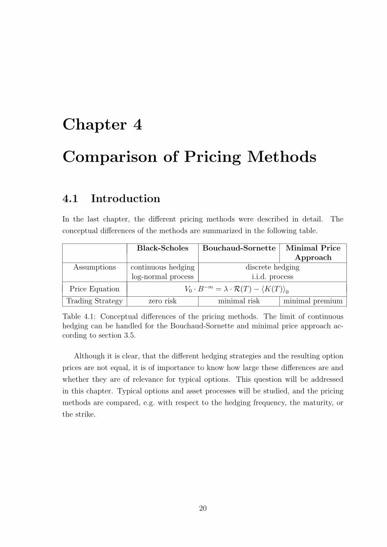
4.1 Introduction

In the last chapter, the different pricing methods were described in detail. The

conceptual differences of the methods are summarized in the following table.

Black-Scholes Bouchaud-Sornette Minimal PriceApproach

Assumptions continuous hedging discrete hedginglog-normal process i.i.d. process

Price Equation V0 ·B−m = λ · R(T )− 〈K(T )〉0Trading Strategy zero risk minimal risk minimal premium

Table 4.1: Conceptual differences of the pricing methods. The limit of continuoushedging can be handled for the Bouchaud-Sornette and minimal price approach ac-cording to section 3.5.

Although it is clear, that the different hedging strategies and the resulting option

prices are not equal, it is of importance to know how large these differences are and

whether they are of relevance for typical options. This question will be addressed

in this chapter. Typical options and asset processes will be studied, and the pricing

methods are compared, e.g. with respect to the hedging frequency, the maturity, or

the strike.

20

Log-Normal Process

p(S, t|S0, t0)1√

2π∆t σ Se−µ2/(2σ2∆t)

µ log(S/S0)− (µ− 1/2 σ2)∆t

∆t 1/250Spot S(0) 50Drift µ 0.1Volatility σ 0.2

Fat Tail Process

p(S, t|S0, t0)2

3

1√2π∆t σG S

e−µ2/(2σ2G∆t) +

80

6e−80·|µ|

µ log(S/S0)− (µ− 1/2 σ2)∆t

∆t 1/250σG 0.15Spot S(0) 50Drift µ 0.1

Volatility σ ≡√

variance ≈ 0.2

Table 4.2: Asset processes for which the pricing methods are compared.

4.2 Asset Processes and Options

4.2.1 The Underlying Process

4.2.1.1 Log-Normal Process

The pricing methods will be compared for two different underlying processes. One is a

log-normal process. For this process, analytic Black-Scholes pricing formulas exist for

continuous time. Comparing the results for discrete hedging with the Black-Scholes

price, reveals the effect of discrete hedging.

The log-normal process for the asset price S is given by

dS = µ S dt + σ S dX (4.1)

with constant drift µ and constant volatility σ. dX = N(0, dt) is a normal random

variable with mean 0 and variance dt. By integration, the probability density to

observe S at time t given a spot price of S0 at time t0 is obtained [2]:

p(S, t|S0, t0) =1√

2π(t− t0) σ Se−(log(S/S0)−(µ−1/2 σ2)(t−t0))

2/(2σ2(t−t0)) (4.2)

The factor 1/S is due to the fact, that the probability density is given for S instead

21

Plain Vanilla OptionMaturity T 0.2 yearsStrike E 50Payoff call max [0, S(T )− E]Payoff put max [0, E − S(T )]

Binary OptionMaturity T 0.2 yearsStrike E 50

Payoff call

{1 if S(T ) > E0 else

Payoff put

{0 if S(T ) > E1 else

General ParametersInterest rate 0.05Price of risk λ 1.1 · λS

Table 4.3: Options for which the pricing methods are compared.

of log S. The values of the parameters S0, µ, and σ, which are chosen for this study,

are shown in table 4.2.

For completeness, the spot price evolution for finite time steps, which is needed

for Monte Carlo simulations, is given here as well [2]:

S(t) = S(t0) e(µ−1/2 σ2)·(t−t0)+σ·[X(t)−X(t0)] (4.3)

4.2.1.2 Fat Tail Process

In section 2.1, it was shown that a log-normal process doesn’t fit to market data. In

data tails are more pronounced, which can be described by an exponential slop. The

second asset model under consideration is a sum of a log-normal and an exponential

function (see table 4.2). The form of the distribution is given by the fit to the IBM

data in section 2.1 and scaled such that the square root of the variance is close to

the volatility value taken for the log-normal process. This guarantees that the option

prices are roughly the same for both processes.

The probability distribution is shown for different time horizons in figure 4.1.

Overlaid is a normal distribution. For short time horizons both distributions show

large differences in the tails, while for large time horizons the fat tail distribution

converges towards the Gaussian distribution, as expected. The convergence is also

22

10-4

10-3

10-2

10-1

1

10

10 2

-0.1 -0.05 0 0.05 0.1log return / sqrt(dt/1 day)

prob

abili

ty d

ensi

ty

asset process

Gaussian dt = 20 days

10-4

10-3

10-2

10-1

1

10

10 2


prob

abili

ty d

ensi

ty

asset process

Gaussian dt = 5 days

10-4

10-3

10-2

10-1

1

10

10 2


prob

abili

ty d

ensi

tyasset process

Gaussian dt = 1 day

Figure 4.1: Probability distributions for the fat tail model for different time horizons.A Gaussian distribution is overlaid to demonstrate the convergence towards a normaldistribution for large time horizons.

23

seen when studying the kurtosis

κ =

⟨(µ− 〈µ〉)4⟩

σ4− 3 (4.4)

of the fat tail distribution which tends to 0 with increasing time horizon. The variance,

on the other hand, scales with dt which is a property of any i.i.d. variable (see section

2.1.2).

4.2.2 Option Characteristics

Since the study focus on the comparison of valuation methods, simple option types

were chosen, for which analytic Black-Scholes solutions [2, 12] exist. Four option

types were considered: European plain vanilla and digital options with call and put

payoff type. The option parameters of table 4.3 are taken as a basis for the different

studies.

Another parameter, to fix for the study, is the price of risk the option writer

charges for the option. A value of

λ = 1.1 · λS (4.5)

was chosen for all studies except for section 3.2. In section 3.2, the dependence of the

option price on the price of risk is studied.

4.3 Software Implementation

4.3.1 Price and Strategy Calculation

4.3.1.1 Solution Algorithm

The first step to determine the option price is to solve the equation

φ∗k =1⟨

∆S2k

⟩k

{⟨V (T )∆Sk

⟩k

(4.6)

+⟨∆Sk

⟩k

[c

λR(T ) +

m−1∑l=0

⟨φ∗l ∆Sl

⟩0− 〈V (T )〉0

]−

n−1∑l=0l 6=k


⟩k

}

with

c = 0 for the Bouchaud-Sornette method (see eq. 3.9),

c = 1 for the minimal price approach (see eq. 3.17).

(4.7)

24

The right hand side of this equation is dominated by the term⟨V (T )∆Sk

⟩k/⟨∆S2

k

⟩k,

if the value Sk is not too far out of the money (see section 3.3.2). This term is inde-

pendent on the hedging strategy. The equation 4.6 is solved by an iteration procedure

with starting values φk =⟨V (T )∆Sk

⟩k/⟨∆S2

k

⟩k

1. In each iteration step, the old

values for φk are substituted on the right hand side of equation 4.6, giving a new set

of values φk.

For each iteration step, the option price, given by equation 3.3

V0 ·Bm = λ · R(T )− 〈K(T )〉0 (4.8)

= λ ·√〈K2(T )〉0 − 〈K(T )〉20 − 〈K(T )〉0

with

K(T ) =n−1∑l=0

⟨φ∗l ∆Sl

⟩0− V (T ) (4.9)

is calculated. If the option price changes from one iteration step to the next by

less than 10−7, the iteration is stopped. For the Bouchaud-Sornette method, the

convergence is usually reached after a few steps. For the minimal price approach,

typically 10 to 20 iterations are necessary.

4.3.1.2 Calculation of Expectation Values

The main effort, in the iteration procedure, is to calculate the expectation values

which are involved in the strategy and price equation. The expectation values are

integrals over the asset price as shown explicitly in appendix A. They are solved

numerically by a Riemann sum approximation. For this approximation, the asset

price is taken to be discrete. Together with the discrete time steps, a grid is defined.

It has the following characteristics:

• The number of mesh points in t is equal to the number of hedges plus one. The

hedging intervals were taken to be equidistant between t0 = 0, for which the

option price is searched, and the option maturity T .

• The asset price is discrete. The mesh has 200 points in S for each time value.

• The points in S are equidistant for each time value, but with different spacing

for different times. The distance between two points is given by the upper and

lower bound for S.

1Another possibility would be to start with the Black-Scholes delta hedging strategy.

25

• The time dependent upper and lower bounds on the asset price are:

Smax(t) =

{S0 +

t

T(S2 − S0)

}· ea (4.10)

Smin(t) =

{S0 +

t

T(S1 − S0)

}· e−a

with

S0 = S(t0)

S1 = min(E, S(t0) · eµT

)S2 = max

(E, S(t0) · eµT

)At time t0 = 0 there is only one mesh point given by the spot value S(t0). The

value of µ is taken from the price process.

The size of the window is mainly determined by the factor a. The fat tail

process needs a larger window for short times, which is taken into account by

the following definition:

a = 6 σ√

t for the log-normal process

a = max(6 σ√

t, 0.25)

for the fat tail process(4.11)

σ is the volatility of the process. Studies similar to the error estimate in section

4.3.3 show that this window size is sufficient.

• For binary options, it is important for reducing numerical errors that the strike

is located in the middle of two grid points. Therefore, the grid points for each

time were shifted, such that the point S0 + (E − S0) · t/T lies in the middle of

two mesh points.

All calculations, except of the calculation for the integral Il|k and the probabilities,

were done in double precision. The integral Il|k is defined in appendix A. Since the

integral Il|k and the probabilities are independent on the hedging strategy, they were

calculated only once per iteration procedure and stored in single precision. Using

single precision reduces the memory consumption considerably, with small effects on

the overall precision.

4.3.1.3 Calculation of Probabilities

For the determination of expectation values, probabilities according to table 4.2 have

to be calculated for different time horizons (see appendix A). For the log-normal

26

process, this is trivial since the explicit formula for all time horizons is known. For

the fat tail process, a distribution is given for a one day time horizon. For larger time

horizons, the distribution has to be convoluted with itself. This autoconvolution was

done by calculating the Fourier transformed, and then taking it to a power which

corresponds to the time horizon, e.g. a power of 2 for two days. At the end, the

inverse Fourier transformation yields the searched probability distribution. This also

allows for time horizons which are not a multiple of one day, e.g. two and a half days.

The Fourier transformation was done with the routine four1 out of reference [13]

which performs a fast Fourier transformation.

Since always the same probabilities are needed in each iteration step, they are

determined only once at the beginning, stored, and reused for the different iteration

steps.

To further improve performance and to reduce the memory consumption, the

integration for the expectation values is done only over the region in S where the

involved probabilities are not negligible. The choice of the grid boundaries in S

are motivated by this idea. In addition, performance improvements are obtained in

the following way. As described above, the integrals of the expectation values are

approximated by Riemann sums. In these sums, only those terms were taken into

account for which the involved probabilities are larger than 1.5 · 10−6. This limit

roughly corresponds to five standard deviations. For the study of implied volatilities

the limit of 1.5·10−6 was reduced to 10−9 since here prices are calculated far out or far

in the money for which the tails of the probability distribution are more important.

The actual values for the limit are justified by the error analysis, described in section

4.3.3. This restriction on the probabilities also reduces the number of integrals Il|k to

be stored and therefore reduces the memory consumption.

4.3.2 Monte Carlo Simulation

Another way to calculate the expectation values is to use Monte Carlo techniques. The

implementation is much simpler, but the calculation is much more time consuming.

Nevertheless, routines for Monte Carlo simulation were coded, to be able to check the

results from the numerical integration and to estimate errors. In addition, the Monte

Carlo simulations were used to generate profit distributions of the hedging portfolio

for illustration.

The Monte Carlo implementation will be described in the following. For the

log-normal asset process uniform random numbers are produced with the standard

27

C function rand(). These random numbers are then transformed to normal dis-

tributed random numbers using the Marsaglia method [2]. For the fat tail process

the acceptance-rejection method [13] was used to generate random numbers, dis-

tributed according to the fat tail distribution. Two uniform random numbers are

taken for each acceptance-rejection test. It turned out, that the random number se-

quence from the Microsoft Visula C++ generator rand() is not free of correlations.

An explanation for the correlation was not found, since the generation algorithm is

not documented. No correlation effects were observed when using the random num-

ber generator ran1() from reference [13]. This generator is an implementation of

the method by Park and Miller with Bays-Durham shuffle. It was used to generate

random numbers for the simulation of the fat tail process. For the log-normal process,

the C generator rand() is sufficient and faster.

As mentioned, the Monte Carlo method was used for the error estimate. For this

purpose, it is essential to know the statistical error of the Monte Carlo result. This

error is obtained by sampling the Monte Carlo events and estimating an error from

the different results of the samples. The error of the full sample is then obtained

by scaling with the square root of the event number. To keep the scaling law, no

acceleration methods, like antithetic variables or moment matching, are used.

4.3.3 Error Estimate

For some of the calculated prices and implied volatilities, errors are quoted in the

following sections. These errors were estimated by studying the variation of results

from different calculations. One set of calculations was done to estimate the uncer-

tainty which comes from numerical errors in the hedging strategy. For each of these

calculations, the determination of the expectation values was changed in one of the

following ways:

• The number of grid points in S was increased from 200 to 300.

• The grid window in equation 4.11 was increased from 6 to 8 standard deviations.

• For the fat tail process, the term max(6σ√

t, 0.25)

in equation 4.10 was replaced

by max(6σ√

t, 0.3).

• Probabilities were taken into account down to values of 1.5 · 10−8, instead of

1.5 · 10−6, for price calculations and down to 10−11, instead of 10−9, for implied

volatilities.

28

• The grid points were shifted in spot direction by 10 % of the spacing in S. The

grid points are then no longer located symmetric around the strike.

For binary options, large effects are expected from such a shift. They are mainly

due to the calculation of the expectation values which enter in the price equa-

tion. Since the focus lies on the error from the hedging strategy, the expected

additional uncertainty from the price equation was eliminated by solving the

price equation with Monte Carlo techniques. For plain vanilla options, the

uncertainty from solving the price equation is small, and therefore the price

equation was solved by numerical integration.

• Probabilities for the fat tail process and arbitrary time horizons were calculated

by a fast Fourier transformation, as explained in section 4.3.1.3. The number

of points used by the fast Fourier transformation was increased from 214 to 216.

For each of these calculations, the deviation of the option price or implied volatility

from the standard result was taken and added quadratic. This gives an estimate of

the error, which will be referenced to as error 1.

In a second step, a Monte Carlo simulation was performed to estimate the error

which comes from solving the price equation 3.3. The hedging strategy was taken

from the standard calculation, and a Monte Carlo sample of 106 events was generated.

From this sample, the option price and the implied volatility was determined. The

difference to the standard result is an estimate of the systematic error. This estimate

only makes sense unless the difference is larger than the statistical error on the Monte

Carlo result. If this condition is not fulfilled, the statistical Monte Carlo error was

taken as a conservative estimate of the systematic error. The statistical Monte Carlo

error was obtained in the way described above, by sampling the 106 events in 20 sets.

The error from the Monte Carlo study will be called error 2.

The two estimates, error 1 and error 2, are combined, by adding them quadratic,

to give the final error. The main contribution to this error is

• for plain vanilla options: the statistical Monte Carlo error.

• for plain vanilla options far in the money (strike = 38): the grid window2.

• for binary options: the systematic error from solving the price equation (error

2). The observed difference between Monte Carlo and the numerical integration

is up to 18 times larger as the statistical Monte Carlo error. This indicates a

2Errors for binary options far out of the money were not determined.

29

RehedgesProcess 5 20 50

Numerical IntegrationBouchaud-Sornette log-normal 4 sec 35 sec 157 sec

fat tails 4 sec 40 sec 159 sesMinimal Price Approach log-normal 4 sec 46 sec 155 sec

fat tails 5 sec 51 sec 341 secboth methods simultaneously log-normal 5 sec 50 sec 184 sec

fat tails 6 sec 56 sec 368 secMonte Carlo Simulation(1 000 000 paths) log-normal 9 sec 26 sec 59 sec

fat tails 194 sec 562 sec 1656 sec

Table 4.4: Performance of the software implementation. The numerical integrationcalculates the hedging strategy and solves the price equation. The Monte Carlosimulation only solves the price equation for a given hedging strategy.

systematic error. However, this error is not as large as it might be indicated by

the factor 18, because the statistical Monte Carlo error itself is small.

The errors are included in different figures in the following sections, e.g. in figure 4.2.

4.3.4 Hardware and Performance

The software was coded in C++ and was run on a Pentium III processor with 750 MHz

and 256 MB RAM. The available RAM memory restricts the number of hedges to 50.

It was not possible to overcome this restriction by using swap memory because in this

case the CPU load drops from about hundred to a few percent. The performance of

the numerical calculations is given in table 4.4. Listed are typical values for the real

time consumption.

4.4 Results

4.4.1 Dependence on the Rehedging Frequency

The Bouchaud-Sornette and the minimal price approach are developed to handle

discrete hedging and non-Gaussian probability distributions. As seen in section 3.5,

the results of the two pricing methods converge towards the Black-Scholes results in

the continuous time limit for a log-normal process. The question arises by how much

the results differ for a realistic process and typical rehedging frequency. This will be

addressed in this section.

30

Figure 4.2 shows results for a plain vanilla call at the money. The option char-

acteristics are as given in section 4.2.2. The risk free interest rate is 5%. Plotted is

the premium, including the risk premium according to equation 3.3, as a function of

the rehedging frequency. For comparison, the standard Black-Scholes price without

risk premium is included in the figure. The Black-Scholes price was calculated with

a volatility equal to the square root of the variance of the asset process.

The other three curves were determined from the price equation 3.3 using the hedg-

ing strategies of the Bouchaud-Sornette method, the minimal price approach and the

Black-Scholes model. The Bouchaud-Sornette strategy and the minimal price strat-

egy were obtained, as described in chapter 3, by minimizing the risk, resp. the option

price. The Black-Scholes strategy is the standard delta hedging which is calculated

analytically with a volatility equal to the square root of the process variance. Errors

for the numerical precision are estimated for the rehedging frequencies of 0.1, 0.4 and

1. The error analysis was explained in section 4.3.3. Most of the errors are smaller

than the marker size and are therefore hidden.

The Black-Scholes and the Bouchaud-Sornette hedging give almost the same re-

sults. The minimal price approach leads to cheaper prices. This was expected since

the price is minimized in this approach. All three curves lie above the Black-Scholes

price without risk premium. For the log-normal asset process, the Black-Scholes price

must be a lower limit for any reasonable model. Otherwise, there would be an arbi-

trage opportunity. For the log-normal process, the convergence towards the risk-free

Black-Scholes price with increasing rehedging frequency is visible. The price gap

remains larger for the fat tail process.

The reason for the larger gap at high rehedging frequencies is explained by figure

4.3. The upper two plots show the risk of the hedging portfolio which enters in the

option price. For the log-normal process, the risk drops much faster with increasing

rehedging frequency. The third plot in figure 4.3 show the contribution of the risk

premium to the option price. The risk premium is roughly twice as large for the

minimal price approach as for the Bouchaud-Sornette method, which is consistent

with the risk distributions. The contribution of the risk premium is of the order of a

few percent of the total price.

The risk, as shown in figure 4.3, is a measure of the width of the profit distribution

at maturity. To get a better understanding of the methods, it is helpful to have a

look at the profit distributions. From the numerical integration procedure, these

distributions are not available. The profit distributions in figure 4.4 were produced

with Monte Carlo simulations. The upper two plots show the profit of the replication

31

2.02

2.04

2.06

2.08

2.1

2.12

2.14

0.1 0.2 0.3 0.4 0.5 0.6 0.7 0.8 0.9 1rehedging frequency [1/day]

prem

ium

Black-Scholes, no risk premium

Black-Scholes

Bouchaud-SornetteMinimal Price Approach

Plain Vanilla Call(at the money, log normal)

2.04

2.06

2.08

2.1

2.12

2.14

2.16


prem

ium


Black-Scholes


Plain Vanilla Call(at the money, fat tails)

Figure 4.2: Plain vanilla call premium as a function of the rehedging frequency fortwo different asset processes. The curves without marker show the standard Black-Scholes price. The curves with marker include a risk premium and are calculated fordifferent hedging strategies. Errors are shown for the rehedging frequencies of 0.1,0.4, and 1. Most of the errors are smaller than the marker size, so that the error barsare hidden.

32

1.75

1.8

1.85

1.9

1.95

2

2.05

2.1

2.15

2.2


prem

ium

Black-Scholes, no risk premiumBouchaud-Sornette, no risk premiumBouchaud-Sornette

Minimal Price Approach, no risk premiumMinimal Price Approach


0

0.25

0.5

0.75

1

1.25

1.5

1.75

2


risk Black-Scholes

Bouchaud-Sornette

Minimal Price Approach


0

0.25

0.5

0.75

1

1.25

1.5

1.75

2


risk Black-Scholes

Bouchaud-Sornette


Plain Vanilla Call(at the money, log normal)

Figure 4.3: The upper two figures show the risk as a function of the rehedging fre-quency. The contribution of the risk premium to the option price is visualized below.

33

-10

-5

0

5

10

15

40 50 60spot at expiry

prof

it

option profit, without risk premium

Bouchaud-Sornettehedging portfolio


-10

-5

0

5

10

15

40 50 60spot at expiry

prof

it

option profit, without risk premium

Minimal Price Approachhedging portfolio


0

20000

40000

60000

-4 -2 0 2 4profit residual

MC

eve

nts

Bouchaud-SornetteMinimal Price ApproachPlain Vanilla Call

(at the money, fat tails)

Figure 4.4: The upper two figures show the profit of the replication portfolio versusthe asset price at expiry, as obtained from Monte Carlo simulation. The lower plotshows the residual distributions, integrated over S(T ).

34

part of the hedging portfolio (the φ dependent part on the right hand side of equation

3.3). Overlaid is the option payoff shifted by the fair option price. The lower plot

shows the residual of the Monte Carlo distribution and the payoff curve, integrated

over the asset price S. The two distributions are consistent with figure 4.3 where the

risk for the minimal price approach was observed to be roughly twice as large as the

risk for the Bouchaud-Sornette approach.

Figure 4.4 also reveals that there is a correlation of the residual with the asset

price for the minimal price approach. We will come back to this point in section 4.4.2

when discussing the differences in the hedging strategies.

In figure 4.5 and 4.6 the same comparison as in figure 4.2 was done for other

option types. The results are similar as for the plain vanilla call option. For options

out of the money, with strike at 55, the difference between the Bouchaud-Sornette

price and the premium from the minimal price approach is larger, up to almost 10

percent of the option price.

4.4.2 Comparison of Hedging Strategies

In the last section, it was pointed out that for the minimal price approach, the profit is

correlated with the spot at expiry (see figure 4.4). In contrast, the Bouchaud-Sornette

method doesn’t show such a correlation. The correlation indicates that more assets

are hold compared to the Bouchaud-Sornette method. This is confirmed by comparing

the hedging strategies directly. In figure 4.7, the hedging strategy φ is shown as a

function of the asset price and time. The figure refers to the plain vanilla call option.

The minimal price strategy requires to hold about 0.2 units of the asset more as

for the Bouchaud-Sornette strategy. The Black-Scholes delta hedging strategy, not

shown in the figure, turns out to be very similar to the Bouchaud-Sornette strategy.

The difference in the strategies can be understood in terms of the portfolio theory.

To see this, consider the Bouchaud-Sornette hedging portfolio as a second asset in

addition to the underlying. The Bouchaud-Sornette hedging portfolio has a “price”

(profit) which is almost uncorrelated with the underlying price S(T ). From portfolio

theory it is known that an investment in two uncorrelated assets gives a better return

to risk ratio as an investment in only one of the two assets. This is, because for a

portfolio of two uncorrelated assets, the return of the assets adds linear while the risk

adds quadratic. This explains why more assets should be hold for the minimal price

approach.

But portfolio theory also points to a possible drawback of the minimal price ap-

proach. The optimal portfolio, in the sense of portfolio theory, is sensitive to the asset

35

1.54

1.56

1.58

1.6

1.62

1.64

1.66


prem

ium


Black-Scholes


Plain Vanilla Put(at the money, fat tails)

1.52

1.54

1.56

1.58

1.6

1.62

1.64


prem

ium


Black-Scholes


Plain Vanilla Put(at the money, log normal)

0.42

0.44

0.46

0.48

0.5

0.52

0.54


prem

ium


Black-Scholes


Plain Vanilla Call(out of the money, fat tails)

Figure 4.5: Plain vanilla option premium as a function of the rehedging frequency fortwo different asset processes. The curves without marker show the standard Black-Scholes price. The curves with marker include a risk premium and are calculated fordifferent hedging strategies. Errors are shown for the rehedging frequencies of 0.1,0.4, and 1. Most of the errors are smaller than the marker size, so that the error barsare hidden. 36

0.51

0.52

0.53

0.54

0.55

0.56

0.57


prem

ium


Black-Scholes


Binary Call(at the money, fat tails)

0.46

0.47

0.48

0.49

0.5

0.51

0.52


prem

ium


Black-Scholes


Binary Put(at the money, fat tails)

0.51

0.52

0.53

0.54

0.55

0.56

0.57


prem

ium


Black-Scholes


Binary Call(at the money, log normal)

Figure 4.6: Binary option premium as a function of the rehedging frequency for twodifferent asset processes. The curves without marker show the standard Black-Scholesprice. The curves with marker include a risk premium and are calculated for differenthedging strategies. Errors are shown for the rehedging frequencies of 0.1, 0.4, and 1.Most of the errors are smaller than the marker size, so that the error bars are hidden.

37

5 10 15 20

4550

5560

0

0.25

0.5

0.75

1

timespot

stra

tegy

Bouchaud-Sornette

5 10 15 20

4550

5560

0

0.25

0.5

0.75

1

timespot

stra

tegy


5 10 15 20

4550

5560

-0.3

-0.25

-0.2

-0.15

timespot

stra

tegy

Bouchaud/Sornette - Minimal Price Approach

Figure 4.7: Comparison of hedging strategies for the plain vanilla call option withthe fat tail asset process. The lower plot shows the difference between the Bouchaud-Sornette and the minimal price strategy.

38

2.1

2.2

0.2 0.3 0.4price of risk

prem

ium hedging strategy:

Black-Scholes without risk premiumBlack-ScholesBouchaud-SornetteMinimal Price Approach

Plain Vanilla Callat the money, fat tails

Figure 4.8: Dependence of the option premium on the price of risk. The rehedgingfrequency is 0.5.

drift, which is more difficult to estimate than the volatility. The methods, described

here, assume a constant drift without any uncertainty. This is obviously only an

approximation. The effect of this approximation will be studied later in section 4.4.5.

4.4.3 Dependence on the Price of Risk

The price of risk λ, taken for the analysis so far, is the price of risk λS from the asset

process, increased by 10 %. As discussed before, the minimal price approach only

makes sense if the price of risk, which enters the minimization procedure, is greater

than λS. If the price of risk tends to infinity, the Bouchaud-Sornette and the minimal

price approach should give the same results (see section 3.4.2.2). Since the Bouchaud-

Sornette strategy doesn’t depend on the price of risk, the Bouchaud-Sornette price

should increase linear with λ. These two effects can be seen in figure 4.8. Shown is the

option price as a function of λ. Compared are the price distributions for the Black-

Scholes, Bouchaud-Sornette, and the minimal price strategies for the plain vanilla call

option. The rehedging frequency is 0.5. The price of risk varies from 1.1 · λS to 4 · λS

in steps of 0.1 · λS.

39

405060

0.10.2

0.3

0.2050.21

0.2150.22

0.2250.23

0.235

strikematurity

impl

ied

vola

tility


Figure 4.9: Volatility matrix for a plain vanilla call and the fat tail process. Thevolatilities are calculated with the minimal price approach. The rehedging frequencyis 0.5 for all maturities.

4.4.4 Implied Volatility Matrix

4.4.4.1 Plain Vanilla Options

The results of section 4.4.1 show that the difference between the option prices, includ-

ing and excluding the risk premium, is larger out of the money than at the money.

Hence, the implied volatility is larger out of the money. This indicates that a volatility

smile is present. A detailed study of the implied volatility is subject of this section.

The implied volatility will be studied in terms of the volatility matrix, that is the

implied volatility as a function of strike and maturity.

The implied volatility is nothing but the option price, transformed into a Black-

Scholes volatility. Inserting the implied volatility in the analytic Black-Scholes for-

mula will return the option price. Figure 4.9 shows, as example, a volatility matrix for

a plain vanilla call. The volatility corresponds to prices calculated with the minimal

price approach including the risk premium. The rehedging frequency is taken to be

0.5, this means one hedge every second day. The typical characteristics, as known

from implied volatilities from market prices, are present in the distribution. A smile

appears, the volatilities increase in and out of the money, and the smile becomes

flatter with increasing maturity. For a quantitative discussion, sectional views, as

in figure 4.10, are more appropriate to use. Therefore, first the strike dependence

(volatility smile) and afterwards the maturity dependence (term structure) will be

40

0.2

0.21

0.22

0.23

40 45 50 55 60strike

impl

ied

vola

tility hedging strategy:


Plain Vanilla Callmaturity = 0.2, fat tails

0.2

0.21

0.22

40 45 50 55 60strike

impl

ied

vola



Plain Vanilla Call(maturity = 0.2, log normal)

Figure 4.10: Volatility smiles for different hedging strategies. On top, results for thefat tail process and on bottom, for the log-normal process are given. Errors are shownfor strike values of 38, 41, 50, and 62. Most of the errors are smaller than the markersize, so that the error bars are hidden.

addressed.

The volatility smile for different hedging strategies is shown in figure 4.10. The

Black-Scholes strategy without risk premium gives, as expected, a constant implied

volatility for the log-normal process. For the fat tail process a smile appears, because

it becomes more likely that the asset price moves from out or in the money into

the strike regime. This effect has been described in the literature, e.g. in reference

[12]. The implied volatilities for the minimal price approach are smaller as for the

Bouchaud-Sornette method. This is obvious since the price is smaller. More surprising

41

0.2

0.205

0.21

40 45 50 55 60strike

impl

ied

vola

tility rehedging frequency:

0.20.40.60.81Black-Scholes limit

Plain Vanilla CallMinimal Price Approach, log normal

Figure 4.11: Implied volatility smile for different rehedging frequencies. The maturityof the option is 0.2. The smile becomes flatter with increasing rehedging frequency.

is the fact that the smile is much more pronounced when the risk premium is included.

This is due to the following effect. The implied volatility far out or far in the money

is mainly determined by the hypothetical asset movements which cross the strike. If

the price is far away from the strike, large price movements for these hypothetical

paths are necessary between each hedge. These large movements result in larger

hedging errors, as for an option at the money. Larger hedging errors gives a larger

risk, and hence, a larger price and a larger implied volatility. This can be verified by

studying the smile as a function of the rehedging frequency, as in figure 4.11. The

smile becomes flatter with increasing rehedging frequency.

For stock options, and here especially for index options, the volatility smile from

market prices is asymmetric[12, 14]. The implied volatilities of call options are larger

in the money than out of the money. One way to model this is by an asymmetric

probability distribution, such that a slump in prices is more likely than an increase

of prices (see [12]). This effect is reproduced in figure 4.12 by setting the fat tail

probability distribution to zero for large positive price changes3.

We are now coming to the discussion of the volatility term structure. For at the

money plain vanilla options, it is shown in figure 4.13. The rehedging frequency is

taken to be 0.5. For the log-normal process, the term structure is flat, while for the

fat tail process, the volatility drops for short maturities even for the Black-Scholes

3The probability distributions are normalized to 1 afterwards and then shifted such that the driftis about 0.1

42

0.2

0.22

40 45 50 55 60strike

impl

ied

vola



Plain Vanilla Callmaturity = 0.2, p(µ > 0.05) = 0

0.18

0.2

0.22

40 45 50 55 60strike

impl

ied

vola



Plain Vanilla Callmaturity = 0.2, p(µ > 0.04) = 0

Figure 4.12: Volatility smiles for asymmetric probability distributions. The proba-bility distributions are based on the fat tail process for which the probability was setto zero above µ = 0.05 (upper plot), resp. above µ = 0.04 (lower plot). Errors areshown for strike values of 38, 41, 50, and 62. Most of the errors are smaller than themarker size, so that the error bars are hidden.

43

0.198

0.2

0.202

0.204

0.206

0.1 0.2 0.3maturity

impl

ied

vola

tility

hedging strategy: Black-Scholes without risk premiumBlack-ScholesBouchaud-SornetteMinimal Price Approach

Plain Vanilla Callat the money, log normal

0.2

0.205

0.21

0.1 0.2 0.3maturity

impl

ied

vola

tility


Plain Vanilla Callat the money, fat tails

0.195

0.2

0.1 0.2 0.3maturity

impl

ied

vola

tility


Plain Vanilla Callat the money, p(µ > 0.05) = 0

Figure 4.13: Term structures for implied volatilities at the money, for different pro-cesses and hedging strategies. The rehedging frequency is 0.5 for all maturities. Thedistributions for a plain vanilla put are similar to the distributions for a call.

44

strategy without risk premium. It can be shown that the effect is much larger than the

numerical errors. Further, the effect is not due to the different number of rehedges at

different maturities because the same effect is observed when the number of rehedges,

and not the rehedging frequency, is taken to be constant for all maturities. The effect

can be understood by the properties of the fat tail distribution and the fact that the

option price at the money is approximatly given by

V (S = E) ≈ 1

2〈|S − E|〉0 (4.12)

where E is the strike. For a log-normal process, this is approximatly equal to V (E) ≈σ0E

√T/√

2π. T is the maturity. For the fat tail process, the expectation value

〈|S − E|〉0 increases faster than√

T . Therefore, the implied volatility increases with

increasing maturity. The term structures for put options, not shown in figure 4.13,

are similar as for call options, and the same argument to explaining the increase of

volatilities with maturity holds.

So far, the volatility matrix was studied as a function of maturity and strike.

For a log-normal process, it is more natural to show the dependence on the variable

log(S/E) ·√

T which enters in the exponential of the probability density. Plotting

the implied volatility as a function of this variable, as in figure 4.14, shows that the

smile is then almost independent on the maturity. For the fat tail process, shown

in figure 4.15, a maturity dependence remains. For larger maturities, the maturity

dependence becomes smaller. This is due to the fact that the fat tail probability

distribution converges towards a Gaussian for large time horizons. At the money, the

implied volatility increases with increasing maturity. This has already been discussed

in relation to figure 4.13. Far out or in the money, the implied volatility decreases

with increasing maturity. In this regime, the option price is sensitive to the tails. The

larger the tails, the higher is the option price. Since the tails decrease with increasing

maturity, relative to a log-normal process, the implied volatility is decreasing in the

tail regions as well. This is somewhat compensated by the risk premium.

4.4.4.2 Binary Options

Volatility matrices for binary options has to be studied separately from plain vanilla

options. This is because the shape of the implied volatility matrix is absolutely

different. Figure 4.16 shows the implied volatility matrix of a binary call for the

minimal price approach with the fat tail asset process. There are two interest-

ing effects visible. First, the implied volatility is larger in the money than out of

the money. And second, for options where the strike is just below the threshold

45

0.202

0.204

0.206

-0.2 -0.1 0 0.1 0.2log(strike/50)*sqrt(0.2/maturity)

impl

ied

vola

tility maturity: 0.032

0.080.1280.1760.224

Plain Vanilla CallMinimal Price Approach, log normal

0.205

0.2075

0.21

0.2125

0.215


impl

ied

vola


0.080.1280.1760.224

Plain Vanilla CallBouchaud-Sornette, log normal

0.198

0.2

0.202

0.204


impl

ied

vola


0.080.1280.1760.224

Plain Vanilla CallBouchaud-Sornette, log normal, no risk premium

Figure 4.14: Volatility smiles at different maturities for a log-normal process. The dis-tributions scale with

√T . Without risk premium, the distribution for the Bouchaud-

Sornette method is flat.

46

0.2

0.21

0.22

0.23


impl

ied

vola


0.080.1280.1760.224

Plain Vanilla CallMinimal Price Approach, fat tails

0.21

0.22

0.23

0.24


impl

ied

vola


0.080.1280.1760.224

Plain Vanilla CallBouchaud-Sornette, fat tails

0.2

0.21

0.22

0.23


impl

ied

vola


0.080.1280.1760.224

Plain Vanilla CallBouchaud-Sornette, fat tails, no risk premium

Figure 4.15: Volatility smiles at different maturities for the fat tail process. Deviationsfrom a

√T scaling is observed for all pricing methods.

47

4050600.1

0.20.3

0.140.160.18

0.20.220.240.260.28

0.3

strikematu

rity

impl

ied

vola

tility


Figure 4.16: Implied volatility matrix of a binary call for the fat tail asset process. Thevolatilities are calculated with the minimal price approach. The rehedging frequencyis 0.5 for all maturities.

d1 =[log(S/E) + (r + 1

2σ2) T

]/σ√

T = 0, where vega dV/dσ is zero, the volatility is

infinite. Just above this threshold, the calculated option price is out of the range of

Black-Scholes prices. An implied volatility doesn’t exist in this regime.

These effects can be understood from the dependence of the Black-Scholes price

on the volatility. In figure 4.17, the Black-Scholes price for a binary call is given for

different volatilities. Supposes that the volatility is 0.2. If one adds a risk premium

to the price, the implied volatility will drop in the money and will rise out of the

money. For relatively small price increases far in the money or just out of the money

no Black-Scholes price exist.

A comparison of implied volatilities from the different pricing models, at a matu-

rity of 0.2, is shown in figure 4.18. This figure corresponds to figure 4.10 and 4.12 for

a plain vanilla call. If volatilities are not plotted in the figure, the price is out of the

Black-Scholes price regime.

4.4.5 Drift Dependence

As described in section 4.4.2, the strategy of the minimal price approach can be

understood in terms of the portfolio theory. The most critical input to portfolio

optimisation is the asset drift. Therefore, the effect of an uncertainty in the drift will

be studied in this section.

48

0

0.2

0.4

0.6

0.8

1

1.2

1.4

35 40 45 50 55 60 65strike

prem

ium

σ = 0

0.10.2

0.5

1.0

2.0

Binary Callmaturity = 0.2, log normal

Figure 4.17: Black-Scholes price of a binary call as a function of strike and volatility.

Using a wrong drift to determine the hedging strategy will result in an unexpected

averaged loss or gain, when applying this strategy. This effect was studied in the

following way. Assume that an option writer has estimated the drift to be 0.1. With

this drift, he calculates his hedging strategy and gets an option price. He also gets an

expected profit from the hedging portfolio. If the real drift is different from 0.1, the

averaged profit will be different as well. This can be quantified by first calculating

the hedging strategy with a drift of 0.1 and then calculating the hedging portfolio

profit with Monte Carlo using a different, the real drift. This simulates that in the

real market the asset process has a drift, different from the one used for the option

pricing. The profit, expected by the option writer, was calculated by using a drift of

0.1. The difference of these two profit values as function of the “real” asset drift, is

shown in figure 4.19. For the Black-Scholes and Bouchaud-Sornette hedging strategy,

almost no drift dependence is observed. The curve for the minimal price approach

shows a slope of about 2 which is in agreement with the following simple estimate.

Due to the additional amount of assets (∆φ ≈ 0.2), the slope is expected to be

∆φ · S(t0) · T = 0.2 · 50 · 0.2 = 2.

Obviously, this introduces a new risk for the minimal price approach, which has not

been taken into account so far. To handle this in a consistent way would require to use

an uncertain drift in the probability distribution. Then, the probability distribution

would be not only a function of the asset price, but also on the drift4. The problem

4In the same way one would extend the method for uncertain volatilities

49

0.15

0.2

0.25

40 45 50 55 60strike

impl

ied

vola



Binary Callmaturity = 0.2, fat tails

0.15

0.2

0.25

40 45 50 55 60strike

impl

ied

vola



Binary Callmaturity = 0.2, log normal

0.15

0.2

0.25

40 45 50 55 60strike

impl

ied

vola



Binary Callmaturity = 0.2, p(µ > 0.05) = 0

Figure 4.18: Implied volatility as a function of the strike for a binary call. Resultsfor different hedging strategies are shown, for the fat tail process, for a log-normalprocess and for an asymmetric probability distribution.

50

-0.1

-0.05

0

0.05

0.1

0.06 0.08 0.1 0.12 0.14asset drift

prof

it

Black-Scholes


Plain Vanilla CallPlain Vanilla Call

(at the money, fat tails)

Figure 4.19: The unexpected averaged profit from the hedging portfolio due to awrong asset drift, taken for the hedging strategy determination. The hedging strate-gies were all determined for a drift of 0.1. The profit difference is shown as a functionof the real drift.

will become more complex, and the calculation of the expectation values would require

additional integrations over the drift. Here only an order of magnitude estimate of

the effect on the price will be given. As example, it is assuming that the uncertainty

on the drift is 2 percent points, so it could be 0.08 or 0.12 instead of 0.1. According

to figure 4.19, this will introduce an uncertainty on the portfolio profit of 0.04. The

risk premium for such an uncertainty is 0.04 · 0.12 ≈ 0.005, where the price of risk

λ = 0.12 is the one used in the previous sections. This additional risk premium has

to be added to the option price. In Figure 4.2 it can be seen that the additional risk

premium reduces the difference to the Bouchaud-Sornette price by roughly 10%. So,

the effect is small, but not negligible.

51

Chapter 5

Conclusions

In this thesis, option pricing was studied with assumptions closer to reality as for

the Black-Scholes method. The continuous time condition was replaced by discrete

hedging, and the restriction of a log-normal asset process was extended to any i.i.d.

process. This pricing problem can be handled in the framework of the Bouchaud-

Sornette method. The method considers a hedging portfolio for which the risk is

minimized.

The Bouchaud-Sornette method was compared to an alternative pricing approach

which was introduced in this thesis. Instead of minimizing the risk, the option price is

minimized in the new approach. The ratio of return to risk for the hedging portfolio

is the same for both methods, by definition. Since the new method minimizes the

price, the hedging strategy of this method allows to write options which are more

competitive on the market.

The two pricing methods were compared for a log-normal asset process and for a

process with fat tails. The main results of the study are the following:

General results

• For a log-normal process in the continuous time limit, both methods recover

the standard Black-Scholes result.

• The option premium of the Bouchaud-Sornette and the minimal price approach

converge towards each other with increasing price of risk.

• For the minimal price approach and the Bouchaud-Sornette method, the ratio of

return to risk for the hedging portfolio is the same, by definition of the methods.

52

• The option premium is smaller for the minimal price approach. Especially for

options far out or in the money, the difference is large. To be competitive on

the market, one should use the minimal price approach.

• If an investor is only interested in hedging the risk, the Bouchaud-Sornette strat-

egy is the optimal choice. In practice, the Black-Scholes delta hedging strategy

is more convenient to use, since it is easier to calculate and the differences are

marginal.

• For both, the Bouchaud-Sornette and the minimal price approach, the risk is

measured in terms of the variance. If an investor has a different view on the

risk, e.g. using the kurtosis, the hedging strategy and the price will be different.

As long as the risk doesn’t vanish, the models always have to make assumptions

on the risk preference.

Results on implied volatilities

• Fat tails in the asset process leads to a volatility smile for plain vanilla options.

• At the money, fat tails give rise to an increasing implied volatility with maturity.

• Including the risk premium in the option price gives a volatility smile for plain

vanilla options. For the options studied, the effect is larger as the one due to

fat tails.

• Asymmetric probability distributions yield asymmetric implied volatility smiles.

• Implied volatility matrices for binary options have a different shape as for

plain vanilla options. Smiles are not present. Implied Black-Scholes volatili-

ties doesn’t exist for all strike values.

Dependence on the asset drift

• The Bouchaud-Sornette method shows almost no dependence on the drift of the

asset. The drawback of the minimal price approach is the drift dependence. It

introduces an additional risk, but the corresponding risk premium is about an

order of magnitude smaller than the price difference between the two method.

53

It has been seen in the study, that both methods are able to reproduce the key

features of implied volatility matrices, as they are observed on the market. The

difference in the pricing methods is that the minimal price approach allows to write

cheaper options. These options are more competitive on the market which is a strong

argument in favour of the minimal price approach.

54

Appendix A

Formulas for Expectation Values

A.1 Strategy Independent Integrals

This appendix contains full formulas for the expectation values which are part of

equation 3.3, 3.9 and 3.17. First, formulas are given for expectation values which are

not strategy dependent. These expectation values have to be calculated only once for

each iteration procedure described in section 4.3.1.

⟨V j(T )

⟩0

=

∫V j(Sm)

m∏i=1

pi|i−1 dmSi =

∫V j(Sm) pm|0 dSm

Il|k =

∫∆Sk pl|k+1 pk+1|kdSk+1

⟨(∆Sk)

j⟩

k=

1

pk|0

∫(∆Sk)

j

m∏i=1

pi|i−1 dSm...dSk+1dSk−1...dS1

=

∫(∆Sk)

jpk+1|k dSk+1⟨V (T )∆Sk

⟩k<m−1

=1

pk|0

∫V (Sm)∆Sk

m∏i=1


=

∫V (Sm)∆Skpm|k+1 pk+1|k dSm dSk+1

=

∫V (Sm) Im|k dSm⟨

V (T )∆Sk

⟩k=m−1

=

∫V (Sm)∆Skpk+1|k dSm

55

A.2 Strategy Dependent Integrals

The following expectation values are strategy dependent and have to be recalculated

for every step in the iteration procedure.⟨φl∆Sl

⟩0

=

∫φl(Sl)

(Sl+1 − Sl

) m∏i=1

pi|i−1 dmSi

=

∫φl ∆Sl pl+1|l pl|0 dSl+1 dSl =

∫φl

⟨∆Sl

⟩lpl|0 dSl⟨

φ0∆S0

⟩0

= φ0

⟨∆S0

⟩0

⟨V (T )φl∆Sl

⟩0

=

∫V (Sm) φl ∆Sl pm|l+1 pl+1|l pl|0 dSm dSl+1 dSl

=

∫V (Sm) φl Im|l pl|0 dSm dSl⟨

V (T )φ0∆S0

⟩0

= φ0

∫V (Sm) ∆S0 pm|1 p1|0 dSm dS1

= φ0

∫V (Sm) Im|0 dSm⟨

V (T )φl=m−1∆Sl

⟩0

=

∫V (Sm) φl ∆Sl pm|l pl|0 dSm dSl

56

For the expectation value⟨φkφl∆Sk∆Sl

⟩0, formulas are only given for k ≥ l since

the expectation value is symmetric in l, k:⟨φkφl∆Sk∆Sl

⟩0

=

∫φkφl∆Sk∆Sl pk+1|k pk|l+1 pl+1|l pl|0 dSk+1 dSk dSl+1 dSl

=

∫dSk dSl+1 dSl φkφl∆Sl pk|l+1 pl+1|l pl|0

∫dSk+1 ∆Sk pk+1|k

=

∫dSk dSl+1 dSl φkφl∆Sl pk|l+1 pl+1|l pl|0

⟨∆Sk

⟩k

=

∫dSk dSl φkφl Ik|l pl|0

⟨∆Sk

⟩k⟨

φ2k∆S2

k

⟩0

=

∫φ2

k∆S2k pk+1|k pk|0 dSk+1 dSk

=

∫dSk pk|0 φ2

k

∫dSk+1 ∆S2

k dSk+1 =

∫dSk pk|0 φ2

k

⟨∆S2

k

⟩k⟨

φk=l+1φl∆Sk∆Sl

⟩0

=

∫φkφl∆Sk∆Sl pk+1|k pk|l pl|0 dSk+1 dSk dSl

=

∫dSk dSl φkφl∆Sl pk|l pl|0


=

∫dSk dSl φkφl∆Sl pk|l pl|0

⟨∆Sk

⟩k⟨

φkφ0∆Sk∆S0

⟩0

=

∫φkφ0∆Sk∆S0 pk+1|k pk|1 p1|0 dSk+1 dSk dS1

=

∫dSk dS1φkφ0∆S0 pk|1 p1|0


= φ0

∫dSk dS1φk∆S0 pk|1 p1|0

⟨∆Sk

⟩k

= φ0

∫dSk φk Ik|0

⟨∆Sk

⟩k⟨

φ1φ0∆S1∆S0

⟩0

=

∫φ1φ0∆S1∆S0 p2|1 p1|0 dS2 dS1

=

∫dS1φ1φ0∆S0 p1|0

∫dS2 ∆S1 p2|1

= φ0

∫dS1φ1∆S0 p1|0

⟨∆S1

⟩1

57

⟨φl∆Sl∆Sk

⟩k=l

= φk

⟨∆S2

k

⟩k

= φk

∫∆S2

k pk+1|k dSk+1⟨φl∆Sl∆Sk

⟩k=l−1

=1

pk|0

∫φk+1∆Sk+1∆Sk

m∏i=1


=

∫φk+1∆Sk+1∆Sk pk+2|k+1 pk+1|k dSk+2 dSk+1

=

∫dSk+1φk+1∆Sk pk+1|k

∫dSk+2∆Sk+1 pk+2|k+1

=

∫dSk+1φk+1∆Sk pk+1|k

⟨∆Sl

⟩l⟨

φl∆Sl∆Sk

⟩k=l+1

=1

pk|0

∫φl∆Sl∆Skpk+1|k pl+1|l pl|0 dSk+1 dSl

=1

pk|0

∫dSk+1 ∆Sk pk+1|k ·

∫dSl φl∆Sl pl+1|l pl|0

=⟨∆Sk

⟩k

⟨φl∆Sl

⟩k⟨

φl∆Sl∆Sk

⟩k=l+1=1

=1

pk|0

∫φl∆Sl∆Skpk+1|k pk|0 dSk+1

= φ0∆S0

∫∆Skpk+1|k dSk+1 = φ0∆S0

⟨∆Sk

⟩k⟨

φl∆Sl∆Sk

⟩k<l+1

=1

pk|0

∫φl∆Sl∆Sk

m∏i=1


=

∫φl∆Sl∆Skpl+1|l pl|k+1 pk+1|k dSl+1 dSl dSk+1

=

∫dSk+1dSlφl∆Skpl|k+1pk+1|k

∫dSl+1∆Slpl+1|l

=

∫dSk+1dSlφl∆Skpl|k+1pk+1|k

⟨∆Sl

⟩l=

∫dSl φl Il|k

⟨∆Sl

⟩l⟨

φl∆Sl∆Sk

⟩k>l+1,l>0

=1

pk|0

∫φl∆Sl∆Skpk+1|k pk|l+1 pl+1|l pl|0 dSk+1 dSl+1 dSl

=1

pk|0


∫dSl+1 dSl φl∆Sl pk|l+1 pl+1|l pl|0

=⟨∆Sk

⟩k

1

pk|0

∫dSl φl Ik|l pl|0 =

⟨∆Sk

⟩k

⟨φl∆Sl

⟩k⟨

φl∆Sl∆Sk

⟩k>l+1=1

=1

pk|0


∫dSl+1 φl∆Sl pk|l+1 pl+1|l

=⟨∆Sk

⟩k

φ0

⟨∆S0

⟩k

58

Appendix B

Continuous Time Limit

B.1 The Limit for Expectation Values

To study the continuous time limit, expectation values

〈f(S, τ)〉 =

∫ ∞

0

f(S, τ)p(S|S0)dS (B.1)

have to be calculated up to first order in ∆t. ∆t = t−t0 is the time difference between

two hedges. The time argument τ of f(S, τ) is equal to t, but is named differently

to avoid confusion when a Taylor expansion of f(S, τ) will be done later. Here, the

continuous time limit will be studied for a log-normal process

p(S|S0) =1√

2πσt Se−1/2·[ln (S/S0)−µ∆t]2/σ2

t (B.2)

with σt = σ√

∆t and µ = µ− 12σ2. First, the variable transformation

y = log (S/S0)− µ∆t ⇐⇒ S = S0 ey+µ∆t =⇒ dS

S= dy (B.3)

is applied. With this transformation, it follows that

p(S|S0) dS =1√2πσt

e−1/2·y2/σ2t dy = p(y) dy

Hence, the expectation value can be written as

〈f(S, τ)〉0 =

∫ ∞

−∞f(y, τ) p(y) dy (B.4)

In the next step, f(y, τ) is replaced by its tailor expansion around y = y0 = −µ∆t

and τ = t0

f(y, τ) =∞∑

n=0

n∑i=0

1

i! (n− i)!

∂nf

∂yi∂τn−i

∣∣∣∣y0, t0

(y − y0)i (τ − t0)

n−i (B.5)

59

which gives

〈f(y, τ)〉 =∞∑

n=0

n∑i=0

1

i! (n− i)!

∂nf

∂yi∂τn−i

∣∣∣∣y0, t0

⟨(y − y0)

i⟩

(τ − t0)n−i (B.6)

For the calculation of the terms < (y − y0)i >, the known moments of the Gaussian

distribution < y2k >= (2k − 1)!! σ2kt and < y2k−1 >= 0 are substituted:

⟨(y − y0)

i⟩

=i∑

j=0

(ij

)⟨yj⟩

yi−j0 (B.7)

=∑

0≤k≤i/2

i!

(2k)! (i− 2k)!(2k − 1)!! σ2k ∆tk (µ∆t)i−2k

=∑

0≤k≤i/2

i! (2k − 1)!!

(2k)! (i− 2k)!σ2k µi−2k ∆ti−k (B.8)

For an expansion up to order ∆t, only terms up to i = 2 have to be taken into account:

〈y − y0〉 = µ ∆t (B.9)⟨(y − y0)

2⟩

= σ2 ∆t + µ2 ∆t2

Substituting this in equation B.6, the expectation value up to order ∆t is

〈f(y, t)〉 = f(y0, t0) +

{∂f

∂τ+ µ

∂f

∂y+

σ2

2

∂2f

∂y2

}∆t +O(∆t2) (B.10)

The inverse transformation from the variable y to S, using

∂f

∂y→ S

∂f

∂S(B.11)

∂2f

∂y2→ S

∂f

∂S+ S2 ∂2f

∂S2

and setting τ = t, gives the final result

〈f(S, t)〉0 = f(S0, t0) (B.12)

+

{∂f

∂t+

(µ +

1

2σ2

)S0

∂f

∂S+

1

2σ2S2

0

∂2f

∂S2

}∆t +O(∆t2)

= f(S0, t0) +

{∂f

∂t+ µ S0

∂f

∂S+

1

2σ2S2

0

∂2f

∂S2

}∆t +O(∆t2)

Here, all derivatives has to be taken at S = S0 and t = t0. This formula will be

applied to different functions f(S, t) in the following.

60

Equation B.12 can be also derived by using Ito’s lemma. For a log-normal process

dS = µS dt + σS dX, the differential df is given by

df =∂f

∂t+

∂f

∂SdS +

1

2σ2S2 ∂2f

∂S2dt (B.13)

Taking the expectation value of this equation, directly yields equation B.12 since

〈dS〉 = µS dt.

All relevant expectation values can now be calculated up to order ∆t:⟨∆S0

⟩0

=⟨S − S0 er∆t

⟩0

(B.14)

= (S0 − S0)− rS0∆t + µS0∆t +O(∆t2)

= S0 (µ− r) ∆t +O(∆t2)

⟨(∆S0

)2⟩

0

=⟨(

S − S0 er∆t)2⟩

0(B.15)

=(S0 − S0 er·0)2

+{2S0r

(S0 − S0 er·0)+ 2µS0

(S0 − S0 er·0)+ σ2S2

0

}∆t

+O(∆t2)

= S20 σ2 ∆t +O(∆t2)

〈V (S, t)〉0 = V (S0, t0) (B.16)

+

{∂V

∂t+ µS0

∂V

∂S+

1

2σ2S2

0

∂2V

∂S2

}S0,t0

∆t +O(∆t2)

⟨V 2(S, t)

⟩0

= V 2(S0, t0) (B.17)

+2

{V

∂V

∂t+ µS0V

∂V

∂S+

1

2σ2S2

0

[(∂2V

∂S2

)2

+ V∂2V

∂S2

]}S0,t0

∆t +O(∆t2)

⟨V (S, t)∆S0

⟩0

=⟨V (S, t)

(S − S0 er∆t

)⟩0

(B.18)

= V (S0, t0)(S0 − S0e

r·0)+

{−rS0V (S0, t0) + µS0V (S0, t0) + σ2S2

0

∂V

∂S

}S0,t0

∆t +O(∆t2)

= S0

{(µ− r) V (S0, t0) + σ2S0

∂V

∂S

}S0,t0

∆t

61

B.2 The Limit for the Hedging Strategy

In this section, it will be shown that the Black-Scholes hedging strategy is a solution

of equation 3.17

φ∗k =1⟨

∆S2k

⟩k

{⟨V (T )∆Sk

⟩k

(B.19)

+⟨∆Sk

⟩k

[1

λR(T ) + 〈K(T )〉0

]−

m−1∑l=0l 6=k


⟩k

}

in the continuous time limit for a log-normal process.

If one substitutes the Black-Scholes strategy in equation B.19, the term propor-

tional toR will vanish in the continuous time limit. This is, because the Black-Scholes

hedging replicates the option in a risk-free way, λ is a constant and⟨∆Sk

⟩k/⟨∆S2

k

⟩k

is finite since the numerator and denominator both are of order ∆t.

Since the Black-Scholes price is uniquely defined for all times, the following relation

can be deduced from equation 2.20:

V (ti) = V (tj>i)−j−1∑l=i

φl∆Sl (B.20)

with V (ti) ≡ V (ti)Bi−m. To see this, one has to take into account that the portfolio

value, Π(t) = ert · Π(t0) = 0, increases with the risk-free rate in the Black-Scholes

world. Hence, it follows for the expectation values⟨V (T )∆Sk

⟩k

=⟨V (tk+1)∆Sk

⟩k+

m−1∑l=k+1

⟨φl∆Sl∆Sk

⟩k

(B.21)

and

m−1∑l=0l 6=k

⟨φl∆Sl∆Sk

⟩k

=m−1∑

l=k+1

⟨φl∆Sl∆Sk

⟩k+

k−1∑l=0

⟨φl∆Sl∆Sk

⟩k

(B.22)

=m−1∑

l=k+1

⟨φl∆Sl∆Sk

⟩k+(V (tk)− V0

)⟨∆Sk

⟩k

Using this and taking into account that V0 = λR − 〈K(T )〉0, equation B.19 can be

written as:

φ∗k =1⟨

∆S2k

⟩k

{⟨V (tk+1)∆Sk

⟩k−⟨∆Sk

⟩kV (tk)

}(B.23)

62

This equation has the same form as equation 3.18. In the same way as in section

3.5, it can be shown that the right side of equation B.23 is equal to ∂V/∂S in the

continuous time limit. The Black-Scholes hedging strategy is therefore a solution of

equation B.19.

63

Bibliography

[1] F. Black and M. Scholes. J. Polit. Econ., 81:637, 1973.

[2] P. Wilmott. Derivatives. Wiley & Sons, 1998.

[3] H.-P. Deutsch. Derivatives and Internal Models. Palgrave, second edition, 2002.

[4] P.J. Hunt and J.E. Kennedy. Financial Derivatives in Theory and Practice. John

Wiley & Sons, 2000.

[5] J.-P. Bouchaud and D. Sornette. J. Phys. I (Paris), 4:863, 1994.

[6] J.-P. Bouchaud, G. Iori, and D. Sornette. Risk, 9:61, 1996.

[7] J.-P. Bouchaud and M. Potters. Theory of Financial Risk. Cambridge University

Press, 2000.

[8] R.N. Mantegna and H.E. Stanley. An Introduction to Econophysics. Cambridge

University Press, 2000.

[9] W. Paul and J. Baschnagel. Stochastic Processes From Physics to Finance.

Springer, 2000.

[10] V. Plerou, P. Gopikrishnan, L.A. Nunes Amaral, M. Meyer, and H.E. Stanley.

Scaling of the distribution of price fluctuations of individual companies. Phys.

Rev., E60:6519–6529, 1999.

[11] P. Jefferies, M.L. Hart, P.M. Hui, and N.F. Johnson. Eur. Phys. J., B 20:493–501,

2001.

[12] J.C. Hull. Options, Futures and other Derivatives. Prentice Hall, 1997.

[13] W.H. Press, S.A. Teukolsky, W.T. Vetterling, and B.P. Flannery. Numerical

Recipes in C. Cambridge University Press, second edition, 1995.

64

[14] R. Cont and J. da Fonseca. Dynamics of implied volatility surfaces. Quantitative

Finance, Volume 2(1), 2000.

65

option pricing for discrete hedging and non-gaussian processes pricin… · both methods were...

Documents