Work supported in part by Department of Energy contract DE-AC02-76SF00515

OPTIMUM ELECTRON DISTRIBUTIONS FOR SPACE CHARGE

DOMINATED BEAMS IN PHOTOINJECTORS

Cecile Limborg-Deprey, Paul R. Bolton

Stanford Linear Accelerator Center, SLAC

MS18 , SLAC. 2575 Sand Hill Road, Menlo Park, CA 94025, USA

Corresponding author: Cecile Limborg-Deprey, limborg@slac.stanford.edu

Stanford Linear Accelerator Center

MS 18, 2275 Sand Hill Road

Menlo Park, CA , 94025, USA

Phone: 650-926-8685

FAX: 650-926-4695

e-mail: limborg@slac.stanford.edu

ABSTRACT

The optimum photo-electron distribution from the cathode of an RF photoinjector producing

a space charge dominated beam is a uniform distribution contained in an ellipsoid. For such a

bunch distribution, the space charge forces are linear and the emittance growth induced by

those forces is totally reversible and consequently can be compensated. With the appropriate

tuning of the emittance compensation optics, the emittance, at the end of photoinjector

beamline, for an ellipsoidal laser pulse, would only have two contributions, the cathode

emittance and the RF emittance. For the peak currents of 50A and 100 A required from the S-

Band and L-Band RF gun photoinjectors discussed here, the RF emittance contribution is

negligible. If such an ellipsoidal photo-electron distribution were available, the emittance at

the end of the beamline could be reduced to the cathode emittance. Its value would be

Contributed to 32nd Advanced ICFA Beam Dynamics Workshop on Energy Recovering Linacs (ERL 2005), 03/19/2005--3/23/2005, Newport News, Virginia

SLAC-PUB-11899

1

reduced by more than 40% from that obtained using cylindrical shape laser pulses. This

potentially dramatic improvement warrants review of the challenges associated with the

production of ellipsoidal photo-electrons. We assume the photo-electrons emission time to be

short enough that the ellipsoidal electron pulse shape will come directly from the laser pulse.

We shift the challenge to ellipsoidal laser pulse shaping. To expose limiting technical issues,

we consider the generation of ellipsoidal laser pulse shape in terms of three different

concepts.

PACS: 29.25.Bx,29.27.Ac,41.60.Cr,41.85.Ar

Keywords: PhotoInjector, Space Charge, Emittance Compensation, Drive Laser, Free Electron

Lasers

2

INTRODUCTION

The lower limit of the emittance of an electron bunch emitted from the photocathode of an

RF gun is the “cathode emittance”. The “cathode emittance” is the product of the rms beam

size and the rms transverse momenta of the photo-electron distribution as it is born at the

cathode. According to the Liouville’s theorem, the emittance is preserved during transport.

However, during transport along a beamline, the different temporal slices of the bunch are

subject to forces of different amplitude. The total emittance grows because of this evolving

mismatch between slices. The mismatch coefficient ξi relates the Twiss parameters of

temporal slice i with those of the total bunch (labeled tot) as follows:

( )itottotitotii γβααγβξ +−= 22/1 (1)

If the forces are linear, (i.e. with respect to the position of the particle in the beam), the

emittance growth is reversible because one can compensate for it. Two examples of linear

forces are linear components of the space charge force and transverse wakefields The former

can be corrected by emittance compensation and the latter by using other transverse

wakefields by steering the beam adequately at the entrance of some linac sections

downstream. For non-linear forces, the emittance growth is usually irreversible. Examples of

non-linear forces responsible for irreversible emittance growth are space charge forces,

incoherent synchrotron radiation emission and RF forces which typically have a sinusoidal

time dependence.

For bunch charges at the nC level, appropriate to X-Ray-FELs, the “cathode emittance”

accounts for half of the total emittance. Of the two other contributions, which combine with

the “cathode emittance” in quadrature, the space charge induced emittance and the RF

emittance, the RF term is negligible. This statement is valid for cylindrical shape laser

pulse.

3

By use of ellipsoidal laser pulse shapes, one suppresses the non-linear space charge forces

and related irreversible emittance growth. The total emittance is then reduced by close to

50% relative to that obtained with a cylindrical pulse shape. The ellipsoidal distribution

affords reduction of cathode emittance by decreasing the radius because the bunch can

tolerate the higher charge density. For the LCLS injector, the slice emittances which are all

above 0.9 mm-mrad for the cylindrical shape are all smaller than 0.6mm-mrad for the

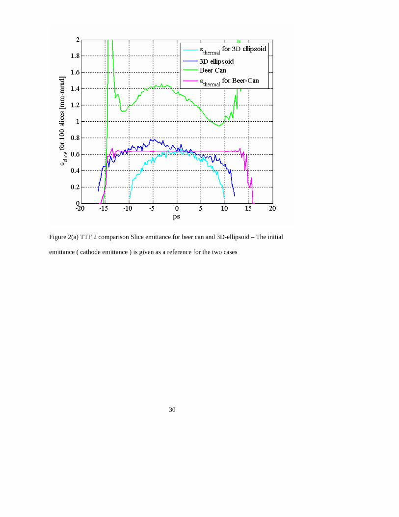
ellipsoidal shape as shown in figure.1a. For the TTF2 injector, results are similarly

impressive where all the slices exceed 1.1 mm-mrad for the cylindrical shape and below 0.7

mm-mrad for the ellipsoidal shape as shown figure 2a.

If this improvement were realized in the X-Ray FEL injectors, the saturation length would be

reduced by 15%, following the standard [1] scaling, which states that the gain length scales

like the third power of the slice emittance. A full start-to-end simulation remains to be done.

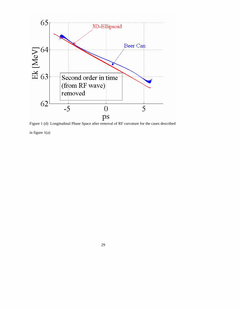
The linear longitudinal phase space, see in figure 1d and the overall improved emittance

match between slices and the very small emittance of the head and tail slices, in contrast to

the cylindrical case, should also improve the performances and facilitate the tuning of the X-

Ray FELs.

Currently, the cylindrical shape is the one of choice for photoinjector drive lasers. The first

part of the paper presents the benefits of the ellipsoidal compared with the cylindrical

distribution in terms of electron beam dynamics. In the second part, we consider the

challenges associated with generating ellipsoidal laser pulses with three different concepts.

2. THEORY- PERFECT EMITTANCE COMPENSATION

2-1 Emittance compensation

Emittance compensation in photoinjectors corrects for linear space charge effects. [2] has

shown that slice mismatches can be minimized with the appropriate choice of fields and

4

location of the solenoid plus accelerator structure. It has also been suggested that one could

compensate for non-linear forces by using non-linear optical components [3-4].

Alternatively, one can suppress the non-linear space charge force components at birth, using

uniform intensity distribution that is contained in an ellipsoidal volume, as described in

equation (2). It is well known that for an ellipsoid with uniform charge density, the space

charge force is linear [5-7]. A bunch that is subject to linear forces will accordingly evolve

keeping an ellipsoidal shape with a uniform charge density inside that volume. It should be

noted that, a recent study [8] shows that starting from a very flat charge pancake at the

photocathode surface an ellipsoidal electron bunch could be self-generated, but this requires

transport of higher peak intensity to the photocathode which can be problematic. In this

paper, we assume that the laser pulse itself would have the ellipsoidal shape and we avoid the

highest intensity laser transport issue.

2-2 Pulse Description

The ellipsoidal distribution is characterized with a constant charge density ρ(x,y,z) inside a

volume that is bound by the following ellipsoid of equation (2) where R is the maximum

radius and L the half of the total bunch length.

12

2

2

2

2

2

=++Lz

Ry

Rx (2)

The line density charge distribution is ( ) ⎟⎟⎠

⎞⎜⎜⎝

⎛−= 2

2

1Lzz oλλ (3)

The maximum radius follows the equation of a semi-circle ( ) 2

2

max 1LzRzr −= (4)

5

The rms radius along the pulse length is ( ) 2

2

12 L

zRzr −=σ (5)

If we ignore the Shottky effect and assume a zero response time for photo-electrons

generation, the photo-electron pulse is identical in shape to the laser pulse and the

requirement on the laser pulses is: a slice laser fluence, Jδ that is uniform in space, constant

along z and within a disk limited by some z dependent maximum radius, ( )zrmax .

The intensity I(r,z) and the power P(z) can then be written

( ) ( )⎟⎟⎠

⎞⎜⎜⎝

⎛⎟⎠⎞

⎜⎝⎛≡

zrrcirc

LzrectIzrI o

max2, (7)

( ) ( )zrIzP o2

maxπ≡ (6)

The slice fluence is then ( ) ( ) tzrIzrJ δδ ,, ≡ (8)

If we make ( )zrmax parabolic then we have:

( )2

2max 1 ⎟

⎠⎞

⎜⎝⎛−≡

Lzzr (9) and ( ) ⎟

⎟⎠

⎞⎜⎜⎝

⎛⎟⎠⎞

⎜⎝⎛−=

22 1

LzRIzP oπ (10)

This means that the longitudinal envelope for intensity is a rectangular shape and the

longitudinal power envelope is parabolic according to the z variation of ( )zrmax . Also, then

the longitudinal envelope of volume space charge density is rectangular but that of the linear

charge density is parabolic.

By contrast, for the cylindrical laser pulse shape the maximum profile radius, rmax is constant

along z so both the intensity and longitudinal power envelopes are rectangular. Furthermore,

those envelopes for both the volume and linear space charge densities are also rectangular.

2-3 Beam Dynamics

6

For an ellipsoid of uniform charge density, the free space potential, in the beam frame, is

given by [9]

( ) ⎟⎠⎞

⎜⎝⎛ +−

−= 22

21

2, zMr

Mzr e

e

oερφ (11) with

⎟⎟⎠

⎞⎜⎜⎝

⎛−⎟⎟

⎠

⎞⎜⎜⎝

⎛−+−

= 111ln

211

2

2

ξξ

ξξξ

eM (12) and ( )2/1 LR−=ξ (13)

The radial and longitudinal electric fields to which a particle at (z,r) is subjected are given by

( ) rLRQfrLRg

E o

o

or γ

ερ

,,,2

12 2

2

−=⎟⎟⎠

⎞⎜⎜⎝

⎛−

−= (14)

zME eo

oz ε

ρ= (15)

The electrical field is independent of the position z along the bunch. The solenoid

compensation can then be perfect. For the cylindrical laser shape, the electric field will

depend on the longitudinal position.

Figures 3 and 4 show simulation results of emittance compensation for ellipsoidal and

cylindrical pulses respectively: (a) the transverse phase space, (b) the longitudinal phase

space and (c) the defocusing parameter r’/r as a function of energy for the beam at exit of the

gun for the first row and at the entrance of the accelerating structure for the second row.

Figure 2, third column, shows that for the cylindrical shape the r’/r is strongly non-linear

with energy, whereas for the ellipsoidal shape it is constant. Therefore as the linear

compensation is performed, the alignment of slices can be perfect for the ellipsoidal case, as

shown in figure 1.

2-3 Multiple contributions to total emittance

7

After emittance compensation, the total emittance writes

2arg

22echspacelinearnonRFcathodetot −++= εεεε (16)

which becomes

2arg

2~ echspacelinearnoncathodetot −+ εεε (17) as the RF emittance is negligible in our

operating range.

2-3-1 Cathode emittance

The “thermal emittance” can be computed based on the laser energy and the surface barrier

potential, and the electron affinity for the semi-conductor cathode material. The “thermal

emittance” per unit spot radius in mm.mrad per mm is equivalent to rms of the transverse

momentum, which is usually expressed in eV. By convenience, we prefer to quote emittance

numbers in mm.mrad per mm of spot size radius. For copper cathode, the “thermal

emittance” per unit spot radius is 0.3 mm.mrad per mm. Several electron beam based

measurements have shown that the “cathode emittance” for copper cathode is closer to 0.6

mm.mrad per mm radius [10-13]. The electron beam measurements show that the value for

the Cs2Te “cathode emittance” is 0.6mm.mrad per mm [14] which is also larger than the

“thermal emittance” estimated to be 0.43 mm.mrad per mm [15].

The reasons for the differences between the “cathode emittance”, which is a measured

quantity, and the “thermal emittance” which is a theoretical value, are not yet clearly

explained. As indicated in equation (18), the surface roughness, the scattering of the

electrons, the oxidation of the surface, the two photon absorption are potential causes.

??222 +++= scatteringroughnessthermalcathode εεεε (18)

[Do the ?? mean to be under the square root? ]

As the “cathode emittance” is proportional to the radius of the laser spot, the smallest viable

radius spot size helps reducing dramatically the emittance. Two mechanisms establish a

8

lower limit to the radius. The first one depends on the maximum surface charge density on

the cathode and is referred to as the “space charge limit” (and is an image charge effect). The

second one is the maximum tolerable space charge force imposed by high charge density.

2-3-2 Space charge limit

The “space charge limit” is set by Gauss’s law, eq. (19). It says that attractive electric field

Es generated from the cathode surface charge density prevents the electron from leaving the

cathode, if this field exceeds the accelerating field Ea. For example, at the 1nC charge level,

it imposes a minimum radius of 0.77 mm and 1.34 mm, respectively for 60 and 20 MV/m

accelerating field. The 60/20 MV/m correspond to the cathode field for a 30degrees launch

phase for peak field of 120/40 MV/m.

oo

s rQEεπε

σ2== (19)

as EE < (20)

ao EQr

πε> (21)

Due to the finite emission time of the 10ps long bunch, the total bunch charge is not present

instantaneously on the surface and this criterion is slightly relaxed as shown in the

simulations and summarized in figure 6.

2-3-3 Non-linear space charge force

The second mechanism imposing a minimum on the radius is the direct space charge force.

9

The charge density and the space charge force increase quadratically with the radius. If the

amplitude of the non-linear space charge force is large, the space charge induced emittance

increase scales like r-2p , with 1<p<2, where r is the laser spot, if no other parameter is

modified. There is no such emittance scaling law for the ellipsoidal case since the non-linear

space charge forces are zero.

Therefore, for the cylindrical shape laser pulse, the optimum radius results from a

compromise between tolerable space charge force, which is synonymous with non-linear

space charge force, and “cathode emittance”. This compromise is summarized as equation

(22).

p

echspacelinearnoncathodetot LrQr

2

22

arg22~ ⎟

⎠⎞

⎜⎝⎛+ −ααε with 1<p<2 (22).

For the LCLS photoinjector, the optimum tuning corresponds to an equal combination of

“cathode emittance” (for 0.7 mm-mrad) and the non-linear space charge emittance (for 0.7

mm-mrad). The total minimum emittance is 1 mm-mrad. A smaller emittance of 0.85 mm-

mrad can be obtained if the “cathode emittance” is reduced to 0.5 mm-mrad by using a

smaller radius of 0.85 mm instead of 1.2 mm. But the laser pulse length has to be stretched to

a 20ps pulse duration [16]. Because of this longer pulse, this solution does not meet the 100A

peak current requirement. The 0.85 mm.mrad is the ultimate minimum for the LCLS injector

run with 1nC because a further reduction of the radius requires longer bunches and thus

increasing the RF emittance to a significant level. The RF emittance grows like the volume

times the bunch length as shown in equation (23).

2-3-4 RF emittance

10

The RF emittance has been described analytically in [17], from which we can extract formula

(23), which shows that the RF emittance is proportional to the product of the beam volume

and the rms bunch length σz.

RFε ~ 22zr

rf

peak

fE

σσ (23)

Since the space charge induced emittance growth can totally be suppressed with ellipsoidal

pulses, a numerical evaluation of the RF emittance can be done by setting the “cathode

emittance” to zero. For the LCLS case, it was determined that the RF emittance is smaller

than 0.15 mm.mrad. Obviously, this method underestimates the RF emittance, as the beam

size σr along the gun is slightly smaller than when the “cathode emittance” has been

included.

3. SIMULATIONS

Numerical results obtained with PARMELA [18] are discussed for the photoinjectors of the

planned LCLS and TESLA X-FEL facilities. The photoinjector beamline for the TESLA

XFEL is presently operated at TTF2. The major parameters for those systems are described

in table 1. The comparison of performances between the cylindrical and the ellipsoidal cases

is done maintaining the peak current of 100A for the LCLS and 50A for the TTF2 case.

3-1 Optimization of LCLS beamline with ellipsoidal pulse

For the LCLS injector, with the cylindrical shape laser pulse, the minimum emittance was

obtained for a combination of a laser pulse duration of 10ps and a 1.2 mm radius at the

cathode. At the cost of reducing the peak current, smaller emittances could be obtained with

longer pulses and smaller radii.

11

The advantage of the 3D-ellipsoid laser pulse is that the charge density of the extracted

photo-electron emitted from the cathode can be increased as the space charge gets totally

compensated for. We explored a wide range of radia from 0.7mm to 1.2 mm, but a smaller

range of laser pulse duration (10 to 12ps) as we wanted to maintain the 100A current as

shown in figure 1b. Results are summarized in figures 6 and 7. It is found that ellipsoidal

laser pulses with radius R smaller than 0.8 mm are not suitable, as expected from the “space

charge limit“ effect discussed earlier. Indeed, for radia smaller than 0.8 mm, the longitudinal

bunch profile gets distorted and it looses its ellipsoidal characteristics. The set of parameters

which give the best solution, i.e. which maximizes the brightness is: a radius R = 0.9mm, 2L

= 10ps and a launch phase of 28 degrees. Comparison of beam performances for the

The optimization of the LCLS beamline (simulations for S-Band gun) was done in searching

the solenoid field and injection phase that yields minimum emittance. The linac gradient as

well as the solenoid and linac positions were unchanged with respect to what is used for the

nominal tuning based on cylindrical laser pulse. For the ellipsoidal pulse, the best injection

phase is 4 degrees lower than that for the cylindrical case at 28 degrees from the 0-crossing.

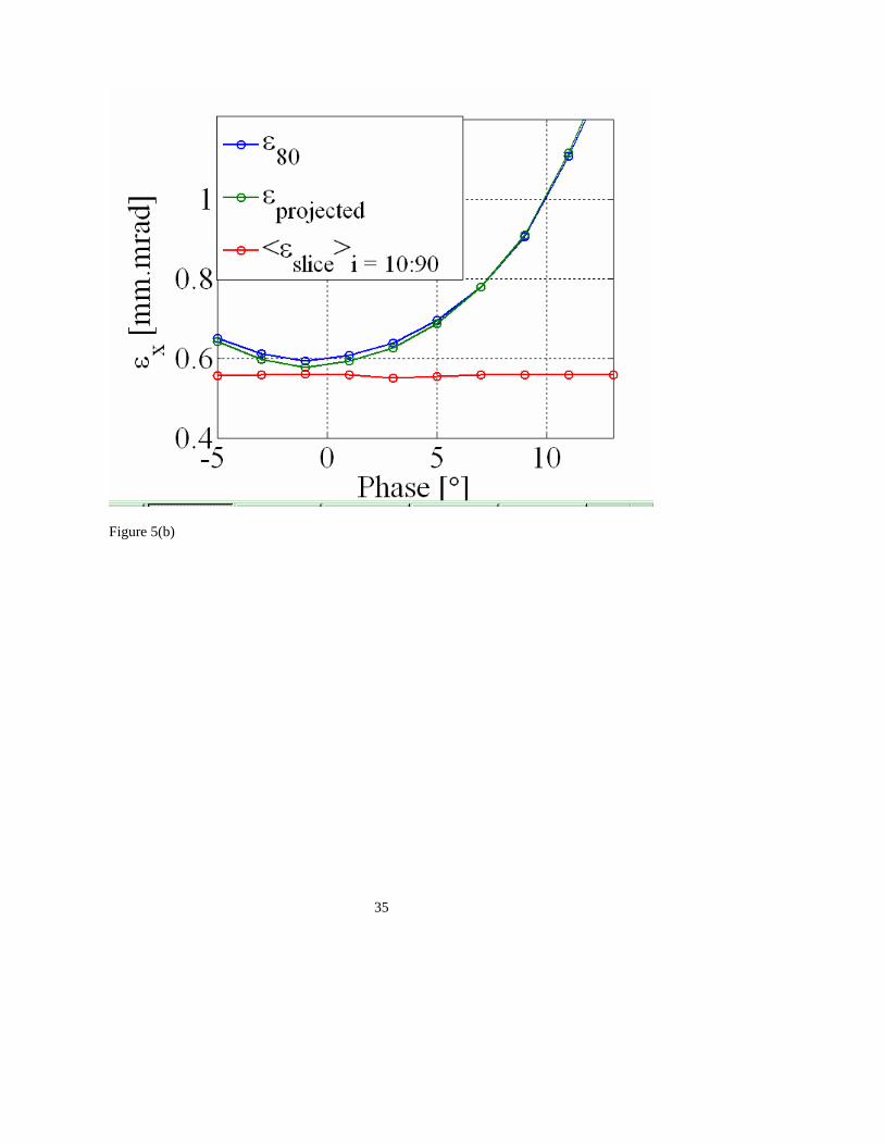
A sensitivity study was performed for the LCLS beamline. The emittance varies much more

slowly with injection phase and solenoid field for the ellipsoidal pulses than for the

cylindrical shape. The variation of emittance with launch phase and with solenoid field are

given in figure 5 for the ellipsoidal pulse. Similar curves are given in [19-20] for the

cylindrical case.

3-2 Optimization of TTF2 beamline with ellipsoidal pulse

The optimization of the TTF2 beamline (simulations for L-Band gun) was also done

by adjusting primarily the solenoid strength and injection phase. The R and L laser pulse

12

shapes were the optimum values determined in the cylindrical case, i.e. a radius R of 1.5 mm

and a pulse duration of 20ps [16]. To achieve perfect emittance compensation, with a final

emittance approaching the cathode emittance value, it was necessary to modify the solenoid

field profile. To facilitate the computation, the same solenoid field distribution was used but

it was shifted longitudinally so that the rising edge would be closer to the cathode by 2.5 cm.

With this modified field profile, a final emittance close to the cathode emittance could be

achieved as shown in figure 8a. A similar field profile could be realistically produced [20].

This result proves that with a gradient field as small as 40MV/m a perfect emittance

compensation can be achieved. Incidentally, running TTF2 with a 60MV/m gradient would

permit operation with smaller R and thus smaller final emittance. We would like to warn the

reader that the simulation results presented here have two issues:

- first the “thermal emittance”, i.e., theoretical value of 0.43 mm.mrad was

used instead of the recently measured “cathode emittance” of 0.6 mm.mrad

per mm

- the reference file used for the cylindrical laser pulse was not perfectly

optimized as suggested by [20].

Those results prove that the final emittance can match the “cathode emittance” in an injector

based on an L-Band gun running at 40MV/m peak current.

3-3 Additional benefits of ellipsoidal laser pulses

The impact of the Shottky effect is reduced with the ellipsoidal case compared with the

cylindrical case. Nonetheless, the small corrections required on the fluence along the pulse

length can be contemplated once shaping techniques are available for ellipsoidal pulses.

13

When the cathode emittance is the only significant emittance source, the emittance scales

with Q1/2 and not Q4/3 as in the high charge regime [22]. This makes the brightness

independent of the charge.

The longitudinal phase space is linear as shown in figure 4. This is beneficial in the

downstream acceleration and compression process. Nonetheless, laser pulse shaping should

then also be considered mindful of downstream issues such as compressor requirements.

4. ELLIPSOIDAL LASER PULSES

In this section we consider longitudinal and transverse laser pulse shaping issues.

With a copper and Cs2Te photocathode in mind one can assume that the central wavelength

is in the UV spectral region (255 nm for example). For other cathode such as GaAs, IR

irradiation would be used. We do not propose a technique for achieving the laser pulse shape

specified in equation (2-10). What is presented here are considerations intended to expose

important technical issues and limitations and to motivate targeted development. We make

reference in what follows to three technical concepts: spectral masking of chirped

waveforms, temporal stacking of multiple laser beamlets, and laser controlled spatial filtering

in a pump-probe configuration.

4.1 Spectral Masking of Chirped Waveforms

The efficacy of spectral masking to control the transverse beam shape and diameter

can be considered in terms the uniqueness of the time-space (one dimensional) correlation

downstream of a diffraction grating in the plane of dispersion. Uniqueness limits are

attributed to the nonzero beamsize projected on the grating and can be evaluated with a

uniqueness function, U. The space-time correlation in question is attributed to the spectrum-

14

time correlation (chirp) of the waveform incident on the grating and the space-spectrum (one

dimensional) correlation established by grating diffraction. More specifically, we consider

position along the intersection of two orthogonal planes; the dispersion plane of the grating

(orthogonal to the direction of its grooves) and a plane parallel to the grating but located at

some distance, D from the grating surface (measured parallel to the grating surface normal).

The appropriate mask is located at this intersection of the two planes (referred to as plane

‘D’) with its long dimension in the plane of spectral dispersion. For a single grating U is

defined as follows:

( ) αδλσ cos

11

Dmaf

fU

≡

+≡

(24)

where m is the order of diffraction

σ is the groove density (per unit length)

δλ is the spectral bandwidth

α is the incident angle on the grating

a is the beam size

For example, the uniqueness is 90% ( U=0.9) for m = 1, σ = 3600 grooves/mm, D = 5

meters, a = 6mm, αcos ≈1, and δλ = 3 nm. This means that the precision of the time-space

correlation in plane ‘D’ is 1-U which is 10% in this case. It is clear that (for a given grating

15

and incident angle,α ) broad spectral bandwidth, small beam size at the grating, and long

distance, D are desirable for maximizing uniqueness.

The mask can then determine beam size and shape for the dimension orthogonal to

the dispersion plane which corresponds to the short dimension of the mask (this is the ‘x’

direction and this mask is referred to as the ‘x’ mask). It is not possible to directly continue

this type of masking in the ‘y’ direction (with a second grating placed immediately after the

first one) without first reconstructing the pulse by recombining the spectrum. This is because

the time-space correlation would no longer be one dimensional after the second grating. After

the ‘x’ masking, we reconstruct the input pulse with a compressor configuration (referred to

as the ‘x’ compressor). The ‘x’ mask in plane Dx would be placed near the second grating of

the ‘x’ compressor.

To shape the ‘y’ dimension we would need a second or ‘y’ compressor configuration

with a ‘y’ mask and a dispersion plane at Dy that is orthogonal to that used with the ‘x’ mask.

The combined pair of compressors does not couple the ‘x’ and ‘y’ beam sizes so the

transverse profile would be rectangular and not circular. The mask size and the large spacing

between the gratings for both the ‘x’ and ‘y’ compressors are critical. The footprint (on an

optical table) of the combined two stage compressor can be reduced by introducing folding

mirrors between gratings for each stage. In our example, four mirrors placed between the

grating pair of each stage can reduce net grating spacing on the table by a factor of five to the

1 meter level.

16

A two stage compressor system like this is characterized by very large temporal

compression of a laser pulse due to its large negative group velocity dispersion (GVD).

Therefore upstream of the compressor pair a stretcher is needed with comparably large

positive GVD to establish the highly chirped input waveform. This stretcher will also be

necessarily large. One can consider a folded or four-pass stretcher system. The combined

group delay established by the stretcher plus compressor determines the chirp of the final

shaped laser pulse that is to irradiate the photocathode. A 10 picosecond UV pulse (of central

wavelength 255 nm) with a 3 nm bandwidth has a chirp of 3 psec/nm (linear estimate). For

example, with the 5 meter spacing, the compressor pair (with 3600 grooves per mm) with

grazing incidence angles can impose time delays +1,763 psec/nm. To obtain the resultant 3

psec/nm chirp, the stretcher would have to generate delays at the -1,760 psec/nm level. In

theory this could be obtained at this UV wavelength with similar gratings to those used in the

compressor stage and with a spacing of several meters. Large diameter optics are required.

Because D is very large, spatial masks will be large. For example, at a 5 meter

distance the long dimension of the mask should be at least 60 mm for a 3 nm bandwidth.

The details of the spatial masks (such as material composition and size limitations) for

application to the UV spectral region are not identified yet. The efficiency of the spectral

masking approach is also of major concern. The mask and grating efficiencies are the

limiting factors. For example, with UV irradiation we anticipate the combined grating

efficiency to be extremely low (of order 10-5) for the folded stretcher plus the two-stage

compressor. It is clear that implementing a spectral masking approach would be expensive,

complicated, large, and inefficient. This combination of attributes can be prohibitive. The

large stretcher plus compressor pair combination is not recommended.

4.2 Temporal Stacking of Multiple Beamlets

17

The pulse temporal stacking approach requires the summation or stacking of multiple

beamlets, each of which has a specified time delay, transverse radius and pulse energy.

Assume that each beamlet is temporally Gaussian but transversely uniform (flattop). Fluence

would then be held constant in time only in a discrete way (beamlet peak-to-beamlet peak).

The summation in the overlap region partially smoothes the discrete fluence levels. Use of a

grating pair provides collimated input to the spectral filter. A spectral mask placed

downstream from the second grating can generate beamlets of durations much less than the

chirped input and each with a slightly different central wavelength. Because the input to the

grating pair for spectral filtering is chirped, an upstream stretcher is also required.

Each beamlet must have its own transverse profile shaper with imaged transport

downstream of the shaper. Each beamlet must also have independent optical delay and

independent pulse energy control. Fluence preservation over all beamlets requires that the

energy of a given beamlet scales linearly with its transverse area. The uniform transverse

profile guarantees constant fluence within any beamlet. In the absence of interference effects

between neighboring beamlets, the temporal envelope of peak intensity should be rectangular

(flattop). However, the peak power temporal envelope should be the same as that of the beam

radius as stated in equation ????.

Interference effects will introduce additional intensity and power variations (ripples)

which can be minimized by alternating beamlet polarization between ‘S’ and ‘P’ cases.

Normally incident photocathode irradiation is desirable if alternating polarizations are used.

Large reflective optics can then be used to steer multiple beamlets to a photocathode with

minimal variation of the incident angle. Beamlets could be grouped into ‘clusters’ with each

cluster using different final reflective optics that are located symmetrically around an

18

electron beamline. Complexity, size and cost can escalate rapidly with the number of

beamlets used (for example, 10 or more). Fluence is not preserved continuously in time.

Interference considerations limit irradiation to normal incidence and their effect can

introduce unwanted ‘ripples’ in the intensity and power temporal profiles. The efficiency of

the combined gratings alone (input stretcher plus grating pair) is at the 10-2 level for UV

wavelengths.

4.3 Laser-Controlled Spatial Filtering

Optically controlled spatial filtering introduces different complexities. We address

briefly issues associated with a pump-probe approach to dynamic spatial filtering in which

the pump pulse is the ‘control’ pulse and the probe pulse is the one that irradiates the

photocathode. Probe shaping attributed to the interaction occurs in the ‘control’ plane. The

anticipated Airy pattern from Fraunhofer diffraction indicates that a uniform transverse laser

intensity profile of circular shape can be formed by Fourier transforming an intensity profile

of the form:

2

1

2

2

⎪⎪⎭

⎪⎪⎬

⎫

⎪⎪⎩

⎪⎪⎨

⎧

⎟⎟⎠

⎞⎜⎜⎝

⎛

⎟⎟⎠

⎞⎜⎜⎝

⎛

∝

o

o

a

faJ

I

λρπ

λρπ

(25)

where a is the desired flat profile radius

ρ is the transverse space coordinate in the control plane

oλ is the central laser pulse wavelength

19

f is an optical focal length

Conceptually, with a given central wavelength, oλ , a focal length, f can be chosen to

establish scaling in the control (Fourier) plane that can be transformed to a flattop circular

profile of radius, a . Requiring this radius to be time dependent (eg. variations on the 100

fsec time scale) means that the pump pulse must be preshaped. The complexity is then two

fold; preshaping the pump pulse and understanding the probe pulse interaction in the control

plane. It is clear that probe pulse shaping would require that preshaping be influenced by the

details of this interaction. The shaping challenge is to generate this complicated Bessel-like

pump profile with appropriate scaling. One could envision reflective and transmissive

versions of this concept.

It is generally known that laser-induced effects can alter transmissive and reflective

behaviour and therefore affect some control of optical properties of materials. However, laser

controlled spatial filtering would require rapid control of refractive indices at high irradiance

levels where material damage is also a major concern. Furthermore, adequately rapid

refractive index dynamics can impose significant spectral shifts and structure on the probe

pulse. It should also be noted that reflective schemes based on semiconductor carrier density

excitation would require very high electron-hole densities (above critical levels which are of

order 1021cm-3 at one micron).

The three concepts discussed above, spectral masking, temporal stacking, and laser

controlled spatial filtering, expose some of the major technical challenges for generating

ellipsoidal laser pulses.

20

5. DISCUSSION AND CONCLUSIONS

This paper has described the great benefits of ellipsoidal photo-electron bunches in

photoinjectors operated in the space charge dominated regime. In this regime, the emittance

will be dominated by the cathode emittance as the space charge emittance is suppressed and

the RF emittance is negligible. Due to the space charge limit, the emittance would follow a

Q1/2 law, where Q is the charge. This would make, in the high charge regime, the brightness

independent of charge. This is of major importance if high flux and average brilliance are the

figures of merit for a facility such as an ERL.

The impressive reduction of close to 50% for both the projected emittance and the

slice emittances, the low sensitivity of the emittance to variation in major parameters and the

linearization of the longitudinal phase space make ellipsoidal photo-electron bunches very

attractive. It has proven that the cylindrical shape is not the optimal laser pulse to drive

space-charge dominated photoinjectors. Producing ellipsoidal laser pulse shapes at the

photocathode remains a challenge that warrants closer examination.

ACKNOWLEDGEMENTS

We would like to thank G.Stupakov and Z.Huang for valuable discussions. We express our

gratitude to K.Floettmann who verified the ellipsoidal optimization for TTF2 using his

ASTRA code. We would like to thank P.Emma and J.Galayda for their support and

encouragements.

21

FIGURE CAPTIONS

Figure 1. Emittance compensation for Ellipsoidal pulse-

Upper row distribution at gun exit (a) transverse phase space (b) Longitudinal Phase Space

(c) r’/r as a function of kinetic energy

Lower row distribution at linac entrance (a) transverse phase space (b) Longitudinal Phase

Space (c) r’/r as a function of kinetic energy

Figure 2. Emittance compensation for cylindrical pulse-

Upper row distribution at gun exit (a) transverse phase space (b) Longitudinal Phase Space

(c) r’/r as a function of kinetic energy

Lower row distribution at linac entrance (a) transverse phase space (b) Longitudinal Phase

Space (c) r’/r as a function of kinetic energy

Figure 3- Comparison of beam properties after optimization between cylindrical (“beer-

can”) and ellipsoidal (“3D-ellipsoidal”) at the end of the beamline

(a) slice emitance (b)peak current (c) ?????? (d) Matching coefficient as defined in equation

(1)

Figure 4- Comparison of longitudinal phase space (after removal of correlation introduced by

RF wave) after the first accelerating structure, between cylindrical (“beer-can”) and

ellipsoidal (“3D-ellipsoidal”) cases

Figure 5- Sensitivity curve- Evolution of emittance as a function of (a) solenoid field and (b)

launch phase – three types of emittance are given : the total projected emittance, the 80%

emittance (i.e. projected emittance for the particles contained in the slice numbered 10 to 90

out of 100) and the average of the 80 central slices (numbered 10 to 90)

Figure 6- Ellipsoidal laser pulse – Evolution of critical parameters (a) peak current, (b) slice

emittance (c) Brightness defined as Ipeak /εslice^2 as a function of rmax ; the pulse length has a

2L value of 10ps and the launch phase is 32 degrees.

22

Figure 7- Evolution of projected emittance as a function of R for two sets of bunch length 2L

(10ps and 12 ps) and two sets of launch phase (28 degrees and 30 degrees)

Figure 8- TTF2 optimization results (a) Slice emittance comparison between the cylindrical

pulse and the ellipsoidal pulse at emission and at end of beamline – (b) comparison of peak

current

23

REFERENCES

[1] M.Xie “Design Optimization for an X-Ray Free Electron Laser Driven by SLAC Linac”,

IEEE Proceedings of PAC 95, No. 95CH3584,183, 1996, LBL Prerpint No-36038

[2] B.Carlsen, “New Photoelectric Injector Design for the Los Alamos Natioanl Laboratory

XUV FEL Accelerator”, NIM A285 (1989) 313-319

[3] J. C. Gallardo and R. B. Palmer, IEEE J. Quantum Electronics 26, 1328-1331 (1990) [4] X.Qiu, K.Batchelor, I.Ben-Zvi, X-J Wang, “Demonstration of Emittance Compensation through the Measurement of the Slice Emittance of a 10-ps Electron Bunch”, Physical Review Letters, Vol 76, Number 20, May13 1996 [5] F.Sacherer, “rms Envelope with Space Charge” IEEE Trans Nucl. Sci. NS-18, 1105

(1971)

[6] I.M. Kapchinskij and V.V.Vladimirskij, Conference on High Energy Accelerators and

Instrumentation , CERN, Geneva (1959), P274

[7] P.M. Lapostolle, “Possible Emittance Increase Through Filamentation due to Space

Charge in Continuous Beams”, IEEE Trans. Nucl.Sci. 18 1101 (1971)

[8] O. J. Luiten, S. B. van der Geer, M. J. de Loos, F. B. Kiewiet, and M. J. van der Wiel

Phys. Rev. Lett. 93, 094802 (2004) [Published 25 August 2004]

[9] M.Reiser “Theory and Design of Charged Particle Beams”, Wiley-Interscience

Publicatiom Editor John Wiley & Sons, Inc.

[10] J.Yang, “Experimental Studies of Photocathode RF Gun with Laser Pulse Shaping”,

EPAC 2002

[11] W.Graves et al. “Measurement of Thermal Emittance for a copper PhotoCathode”, PAC01 Proceedings

Deleted: O.J.Luiten et al. ““How to realize uniform 3-dimensional ellipsoidal electron bunches”, Phys. Rev. [Please provide complete reference] August 2004

24

[12] D.H. Dowell, P.R. Bolton, J.E. Clendenin, P. Emma, S.M. Gierman, W.S. Graves, C.G.

Limborg, B.F. Murphy, J.F. Schmerge, "Slice Emittance Measurements at the SLAC Gun

Test Facility." SLAC-PUB-9540 (September 2002)

[13] J.F. Schmerge, P.R. Bolton, J.E. Clendenin, D.H. Dowell, S.M. Gierman, C.G. Limborg,

B.F. Murphy, "6D Phase Space Measurements at the SLAC Gun Test Facility." SLAC-

PUB-9681 (January 2003)

[14] V.Mitchell “Thermal Emittance Measurments”, ICFA X-Ray FELs Commissioning

workshop, Zeuthen April 2005

http://adweb.desy.de/mpy/ICFA2005_Commissioning/Talks(PDF)/

[15] K.Floettmann “Note on the Thermal Emittance of Electrons Emitted by Cesium

Telluride Photo Cathodes”, Feb 1997, TESLA-FEL, 97-01

[16] C.Limborg-Deprey et al. “Modifications of the LCLS PhotoInjector Beamline” EPAC 04 Proceedings, Lucerne, July 2004 [17] K.J.Kim “RF and space charge effects in laser driven RF electron guns”. NIM in

Physics Research A275 (1989) 201-218

[18] PARMELA ?????,L.Young, J.Billen , PARMELA, LANL Codes,

laacg1.lanl.gov/laacg/services/parmela.html

[19] C.Limborg “New Optimization for the LCLS PhotoInjector Beamline” EPAC 02 Proceedings, Paris, June 2002 [20] C.Limborg-Deprey et al. , NIM A528, 2004, 350-354 [21] K.Floettmann « Private Communications »

[22] J.Rosenzweig, E.Colby, “Charge and Wavelength Scaling of RF Photoinjector Designs” American Institute of Physics 1995, P724

Formatted: English (U.S.)

25

Figure 1(a)

26

Figure 1(a)

27

Figure 1(b ) Pseudo Brightness defined as ratio of peak current over emittance for the two

cases described in figure1 (a)

28

Figure 1(c) Matching Parameter for the two cases described in figure 1a

29

Figure 1 (d) Longitudinal Phase Space after removal of RF curvature for the cases described

in figure 1(a)

30

Figure 2(a) TTF 2 comparison Slice emittance for beer can and 3D-ellipsoid – The initial

emittance ( cathode emittance ) is given as a reference for the two cases

31

Figure 2(b) Comparison peak current for the cases described in Figure 2(a)

32

33

Figure 3 Emittance compensation for a cylindrical beam

Figure 4- Emittance compensation for a 3D-ellipsoidal laser pulse

Figure 4.

34

Figure 5(a)

35

Figure 5(b)

36

Figure 6

37

Figure 7

38

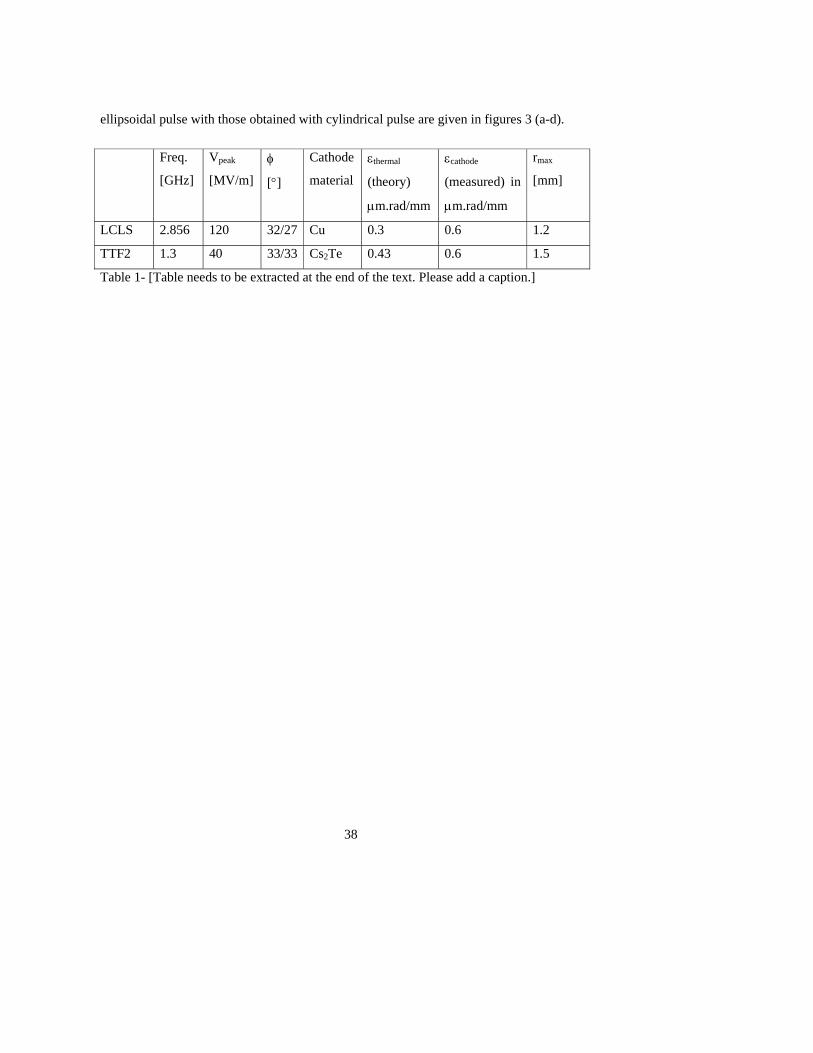
ellipsoidal pulse with those obtained with cylindrical pulse are given in figures 3 (a-d).

Freq.

[GHz]

Vpeak

[MV/m] φ

[°]

Cathode

material

εthermal

(theory)

μm.rad/mm

εcathode

(measured) in

μm.rad/mm

rmax

[mm]

LCLS 2.856 120 32/27 Cu 0.3 0.6 1.2

TTF2 1.3 40 33/33 Cs2Te 0.43 0.6 1.5

Table 1- [Table needs to be extracted at the end of the text. Please add a caption.]