OptiMoS: Optimal Sensing for Mobile SensorsZhixian Yan⇤, Julien Eberle†⇤, Karl Aberer⇤

⇤ EPFL, Switzerland† Nokia Research Center, Lausanne, Switzerland

E-mail: zhixian.yan@epfl.ch, julien.eberle@nokia.com, karl.aberer@epfl.ch

Abstract—Both sensor coverage maximization and energy cost

minimization are the fundamental requirements in the design ofreal-life mobile sensing applications, e.g., (1) deploying environ-mental sensors (like CO2, fine particle measurement) on publictransports to monitor air pollution, (2) analyzing smartphoneembedded sensors (like GPS, accelerometer) to recognize peopledaily activities. However sensor coverage and energy cost con-tradict each other: the higher frequency mobile sensing takes,the more energy is used; and vise versa.

In this paper, we design a novel two-step mobile sensingprocess (“OptiMoS”) to achieve optimal mobile sensing that caneffectively balance sensor coverage and energy cost. In the firststep, OptiMoS divides the continuous mobile sensor readings intoseveral segments, where the readings in one segment are highly-correlated rather than readings amongst different segments. Inthe second step, OptiMoS identifies optimal sampling for thesensor readings in each segment, where the selected readings canguarantee reasonably high sensor coverage with limited samplingrate. Various greedy & near-optimal segmentation and sampling

methods are designed in OptiMoS, and are evaluated using real-life environmental data from mobile sensors.

I. INTRODUCTION

Wireless sensor networks (WSN) and publishing of sen-sor data on the Internet bear the potential to substantiallyincrease public awareness and involvement in environmentalsustainability. Air quality monitoring in urban areas is a primeexample of these applications as common air pollutants havedirect effects on the human health. Traditional WSN basedenvironmental monitoring systems (like SensorScope [12] andMacroScope [26]) typically deploy sensors on some pre-selected positions, monitor these fixed sensors, and analyzetheir measurements. These traditional environmental monitor-ing systems based on static WSN using fixed sensors have acouple of obvious limitations, e.g.,: (a) the system is inflexiblefor monitoring location-varying environment as the sensorplacement is pre-fixed; (b) it is expensive to deploy andmaintain a large set of static sensors; (c) for monitoring avery large area, it is impossible to get enough static sensorsto cover the complete area.

To overcome such limitations of using static WSN forenvironmental sensing, researchers recently start to build WSNwith mobile sensors. There are a lot of emerging mobilesensing platforms, e.g.,: (a) the OpenSense project in Switzer-land builds sensors and deploys them on public transportslike buses and trams [2]; (b) the floating sensor networkproject at UC Berkeley builds a water monitoring system usingdrift sensors to analyze water contaminant [1]; (c) mobilephones are used to establish a community seismic network

to detect earthquakes and rare events [9]. These projects usemobile sensors and bring public involvement in environmentalmonitoring to a reality, which poses today substantial researchand technical challenges for the communication and infor-mation systems infrastructure, to scale up from isolated wellcontrolled systems to an open and scalable infrastructure.

For traditional static WSN applications (e.g., environmentalmonitoring and others), we need to find the best places to fixthese limited sensor resources (e.g., the number of sensors)that can maximize sensor coverage. This is the fundamentalsensor placement problem of WSN; and a good placementcan guarantee the coverage and reflects how well an areais monitored by sensors. Determining an optimal sensingplacement in an arbitrary sensor field is a kind of art galleryproblem, which is NP-hard [18] and requires near-optimalsolutions like the submodularity method [15].

Regarding mobile sensors based environmental monitoring,sensor placement is even more challenging compared to staticWSN; this is because mobile sensors have varying coveragedue to their mobility. In the OpenSense project, we deployenvironmental sensors on moving buses to monitor air quality(using sensors to measure CO2, CO, NO2 etc.), which aremobile sensors as the buses are regularly running on the road.In OpenSense, there are two levels of objectives for optimalsensor placement: the first one is to build the optimal mobilesensing for each individual bus line, i.e., determining whenand where the bus should take a measurement; the second oneis to build global optimal sensing, which provides optimalsensing for all bus lines, where individual sensing on one busline should consider nearby bus lines. For example, Fig. 1shows optimal mobile sensing of four bus lines, where thetimes symbol (“⇥”) indicates the sensing points when andwhere the bus pass by. In such mobile sensing planning, Bus 3only has two sensing points (blue “⇥”), as there are severaloverlapping sensing points with other buses. In this paper, wefocus on the first mobile sensing objective of OpenSense, i.e.,the optimal sensing strategy for each individual moving bus.

Research Questions: We seek to design an optimal mobilesensing strategy, which offers an appropriate tradeoff between“sensing coverage maximization” and “sensing cost (sampling)minimization” of an individual moving sensor. This raises twokey research questions:

a) For a short sequence of mobile sensing (e.g., a movingbus in 2 hours), how to find an optimal sensing (orsampling) protocol which can guarantee required sensorcoverage using limited sensing cost (or sampling rate)?

Bus$1 Bus$2

Bus$4 Bus$3

sensing$point$on$the$bus

Fig. 1: Mobile sensing via moving buses with environmental sensors

b) For a long sequence of mobile sensing (e.g., a movingbus in one month or several days), how to find optimalsensing? Do we need to do segmentation first? Cansegmentation help to make better sensing (sampling)?

Key Contributions: To address these questions, this paperutilizes real-life mobile sensing data of environmental monitor-ing from the OpenSense project. We propose a model-drivenoptimal sensing strategy for mobile sensors. The detailedcontributions of this paper are as follows:

a) We design “OptiMoS”, a two-tier optimal sensing frame-work for mobile sensors, using model-driven data regres-sion (e.g., linear model, support vector regression). Inthe first tier, a long sequence of mobile sensing (e.g.,the complete route of a bus line) is divided into severalnon-overlapping segments, where the data points in eachsegment are homogeneous in terms of modeling andprediction. In the second tier, OptiMoS chooses optimalsampling points for each segment, as these data pointscan provide maximum sensor coverage.

b) For segmenting sensing data from mobile sensors, wedesign and compare several different segmentation algo-rithms, from the optimal exhaustive search using dynamicprogramming, to the binary top-down segmentation, tothe near-optimal error-based heuristic segmentation.

c) For sampling the sensor readings in each segment, wedesign and compare several sampling algorithms, includ-ing the uniform, random, error-based entropy sampling,and the near-optimal mutual-information sampling.

d) To validate such optimal mobile sensing method of Opti-MoS, all of these segmentation and sampling algorithmsare exhaustively evaluated using real-life environmentalsensing data from the moving buses.

The detailed structure of this paper is organized as follows:after the introduction, Section II summarizes existing relatedworks; Section III describes the preliminaries and the two-tieroptimal sensing framework of OptiMoS; Section IV presentsdifferent segmentation algorithms for dividing mobile sensingstream; whereas Section V proposes different sampling strate-gies for individual segment; in Section VI, we experimentallyevaluate the OptiMoS. Finally, Section VII includes conclud-ing remarks and points to future works.

II. RELATED WORK

There are three main topics related to this paper: (1) optimalsensor placement in static WSN; (2) mobile sensing; and (3)sensor data segmentation.

Sensor Placement in WSN: Sensor placement has a signif-icant influence in building an efficient wireless sensor networkfor environment monitoring. An optimal sensor placementshould be able to maximize the sensor coverage and in themeanwhile to minimize the number of sensors required. Forplacing K sensors optimally in an arbitrary sensor field, thiswork is known to be NP hard; thus a couple of efficient near-optimal algorithms are provided [17][20][7][21]. In Andreas’works like [17], a greedy solution is designed by using mutualinformation when selecting next sensor point; this has betterperformance than traditional random solution or other basicentropy-based sensor selection. In [20], the sensor placement ismodeled as a min-max optimization problem, and a simulatedannealing based algorithm is provided. In [7], the methodsupports imprecise sensor detection like terrain properties,which can support sensor placement with probabilistic guar-antee in a polynomial time. The work of regions sampling in[21] studies local aggregation on sensor network and buildsadaptive sampling for each partial region. All of these worksare not designed for mobile sensors. Nevertheless, relevantoptimization formulation and greedy solutions can be adoptedin OptiMoS, to achieve optimal sensing of an individualmoving bus with deployed environmental sensors.

Sensing from Mobile Sensors: Recently, there has beenemerging a number of mobile sensing applications, particularlyin urban computing, such as OpenSense for air quality mon-itoring [2], floating sensors for water contaminants analytics[1], and community sensing for road traffic monitoring [16].One recent work similar to our optimal sensing objective inOpenSense is the Ear-Phone [25], which provides an end-to-end participatory urban noise mapping system and gener-ates a noise map from a small set of sensor readings at asparse spatio-temporal sensing field. Similarly, our objective inOpenSense is to provide a time-varying air pollution map fromlimited mobile sensor readings using a small number of mov-ing buses with deployed environmental sensors (e.g., CO2).However, our work in OpenSense has additional challenges:(a) the monitoring area in OpenSense is not 1D road line like[25], but a 2D map and even 3D earth; and (b) OpenSense isreal mobile sensing that deploy sensors on the moving buses,whilst Ear-Phone fixes mobile phones aside the road.

Sensor data segmentation: Segmentation is largely stud-ied in time series [14][13][11] and GPS-alike mobility data[27][5]. Segmentation methods are divided into three cate-gories, i.e., sliding window, top-down and bottom-up. Slidingwindow algorithms can work online and efficiently, but the re-sults are poor and sensitive to parameters; whilst top-down andbottom-up methods have better segmentation results but not forreal-time applications. To balance both offline high-accuracyand online efficient-computation, a couple of combinationalgorithms are proposed, such as SWAB (Sliding WindowAnd Bottom-up) [13], amnesic functions [23], piecewise linearsegmentation (mixing both constant and linear function) [19],FSW (Feasible Space Window) & SFSW (Stepwise FSW)[22], SwiftSeg (a polynomial approximation of a time seriesin either sliding or growing windows) [10]. In this paper,

we study different segmentation methods, test them with thecombination of different sampling strategies, and evaluate theoptimal sensing proposal of OptiMoS.

III. TWO-TIER OPTIMAL MOBILE SENSING

This section presents our two-tier optimal mobile sensingproposal (i.e., OptiMoS) and its problem formulation. Fig. 2sketches the framework of OptiMoS for achieving the optimalsensing, as well as the data flow in this procedure.

Sensor Readings

Optimal Segmentation

Optimal Sampling

S1 S2 S3 S4 S5

Layer&I.&Op+mal&Segmenta+on&(Modeling*by*Linear,*Polynomial,*SVM*Regression,*ARIMA*modeling*etc.*)*

Layer&II.&Op+mal&Sampling&(Op?mal*sampling*on*each*segment)*

Fig. 2: OptiMoS’s two-tier optimal sensing framework

In the lower tier of OptiMoS, initial input is the raw sensorreadings collected by moving sensors, i.e., multiple dimen-sional spatio-temporal time series data. Each reading recordis the “⇥” symbol in Fig. 2 (i.e., Ri = ht, l, x1, · · · , xmi),which includes sensing time t, sensing location l (typicallyhlongitude, latitudei from GPS), and environmental mea-surements x1 to xm

1. The objective of this tier is to findthe optimal (or near-optimal) segmentation based on datamodeling on these raw readings. OptiMoS can support allkinds of modeling methods, e.g., simple linear regression,polynomial regression, SVM (Support Vector Machine) basedregression, time series ARIMA (Auto-Regressive and MovingAverage) modeling. As the result of the first tier, we canachieve an optimal (or near optimal) segmentation, e.g., fivesegments (from S1 to S5 in Fig. 2).

In the upper tier of OptiMoS, we focus on studying indi-vidual segments that are computed from the lower tier. Foreach segment, the objective is to find the best sampling fromthe mobile sensor readings, i.e., to select only a subset ofsensor readings (“⇥” symbols in Fig. 2 in the top layer). Thissubset can keep enough modeling information for regressionof the whole segment and for prediction of non-selected sensorreadings. Taking Fig. 2 for example, from segment S1 to S5,we respectively keep only 1, 3, 3, 2, 3 readings to achievereasonably enough sensing. For this optimal sensing example,OptiMoS only requires 12 sensing points instead of the initial21 points. The sampling rate is 12/21, i.e., 57%.

A. Problem Statement

As mentioned, the OpenSense project has two levels ofoptimal sensing objectives, i.e., local optimal sensing for

1Taking air quality monitoring using environmental sensors for example,x1 is the measurement of CO2, x2 is of CO, x3 is of NO2, etc.

individual bus line, and global optimal sensing for multiple buslines. In this paper, we focus on the first objective and designOptiMoS (the two-tier optimal sensing) for mobile sensors interms of a single bus line.

This optimal sensing problem can be formulated as fol-lows: Given a sequence of initial mobile sensor readingsR = {R1, · · · , RN} of size N from continuously mov-ing sensors, where each record Ri = ht, l, x1, · · · , xM iconsists of M types of sensor readings (from x1 to xM )together with the timestamp (t) and the location (l =hlongitude, latitude, altitudei), the objective of OptiMoS isto identify the best sampling of such sequence of sensorreadings that can guarantee the majority of sensor readinginformation (i.e., sensor coverage maximization) at the mini-mum sampling rate (i.e., energy cost minimization).

As shown in Fig. 2, our solution for this problem is toprovide a two-tier optimization framework. We will comparethis with traditional one-tier sampling without segmentation,and further details will be provided in Section VI.

B. Optimal SegmentationAs the first tier of OptiMoS, optimal segmentation on

the initial reading sequence (i.e., R) is to find the bestK segments (i.e, R1,R2, · · · ,RK) such that the sum ofthe model errors for individual segment is minimized. Amodel M on a segment Ri can be linear, polynomial, SVMregression, ARIMA etc. In this paper, we empirically studylinear and SVM regression, and evaluate their performances;other models could have similar principle. We apply the RSS(Residual Sum of Squares) to quantify the error for modelinga sequence R = {R1, R2, · · · , RN} (see Formula 1). Theresidual res(Ri) of a reading Ri is the difference betweenreal value in Ri and the approximation Ri that learnt by themodel M(R).

RSS(M(R)) =NX

i=1

(res(Ri))2 =

NX

i=1

(|Ri � Ri|)2

where Ri = M(R)|Ri (1)

Finding the best K segments is equivalent to identifying thebest K-1 division points: Rd1 , Rd2 , · · · , RdK�1 ; then, for eachsegment Ri, we have a sub sequence of readings between twodivision points, i.e, Ri = {Rdi�1 , Rdi�1+1, · · · , Rdi}. For thefirst segment (R1), Rd0 indicates the first reading R1. Now,this optimal segmentation problem becomes an unconstrainedoptimization problem (see Formula 2).

argmind1,d2,··· ,dK�1

KX

i=1

RSS(M({Rdi�1 , · · · , Rkdi})) (2)

Ideally, the segment number (K) is not known in advance,which needs to be discovered automatically as a part of theoptimization problem, as shown in Formula 3.

argminK,d1,d2,··· ,dK�1

KX

i=1

RSS(M({Rdi�1 , · · · , Rkdi})) (3)

For simplicity, in the first step of this work, we can assumeK is given and we will test a reasonably small set of differentK values (e.g., K 10 in our experiment), to analyze theconvergence of segmentation algorithms and to test a near-optimal segmentation.

C. Optimal Sampling

After getting the optimal segmentation, OptiMoS needs toidentify the best sampling of mobile sensing/readings for eachindividual segment. To quantify whether a sampling readingsequence Rsub is good or not, we define “information loss”L(R,Rsub), i.e., the RSS increase ratio between Rsub andthe complete readings R.

L(R,Rsub) =RSS(M(Rsub ! R))�RSS(M(R))

RSS(M(R))⇥ 100(%)

=

NX

i=1

(Rk �M(Rsub)|Rk )2 �

NX

i=1

(Rk �M(R)|Rk )2

NX

i=1

(Rk �M(R)|Rk )2

(4)

where, RSS(M(Rsub ! R)) means the RSS error for theapproximation of the complete sequence R by using the modelM(Rsub) that learnt from the sub sequence Rsub.

Similar to reformulating the sensor placement problem instatic WSN, there are two ways to represent the optimalsampling problem in OptiMoS: (1) Given a limited samplingrate �, find the best sampling set Rsub that has minimuminformation loss L(R,Rsub); and (2) Given an acceptableinformation loss threshold ✏ between sampling sub-sequenceRsub and the complete sequence R, find the best samplingpoints that has the minimal sampling rate. They are formulatedas the following two optimization problems respectively.

argminRsub

L(R,Rsub) s.t. |Rsub|/|R| � (5)

argminRsub

|Rsub|/|R| s.t. L(R,Rsub) � ✏ (6)

The sampling rate |Rsub|/|R| is the sensing frequency, as akind of mobile sensing cost. Thus, the optimal mobile sensingneeds to balance the information loss (i.e., sensor coverage)with the sampling frequency (i.e., the energy cost). The pre-vious two constraint optimization problems in Formula 5 andFormula 6 can be rewritten as an unconstrainted optimizationin Formula 7, by using a balance coefficient �.

argminRsub

L(R,Rsub) + �|Rsub| (7)

IV. SEGMENTATION OF MOBILE SENSING

This sections present various segmentation strategies inOptiMoS, from optimal segmentation by exhaustive search likedynamic programming, to top-down binary segmentation, toerror-based heuristic and near-optimal segmentation. This isto solve the optimization problem in Formula 2.

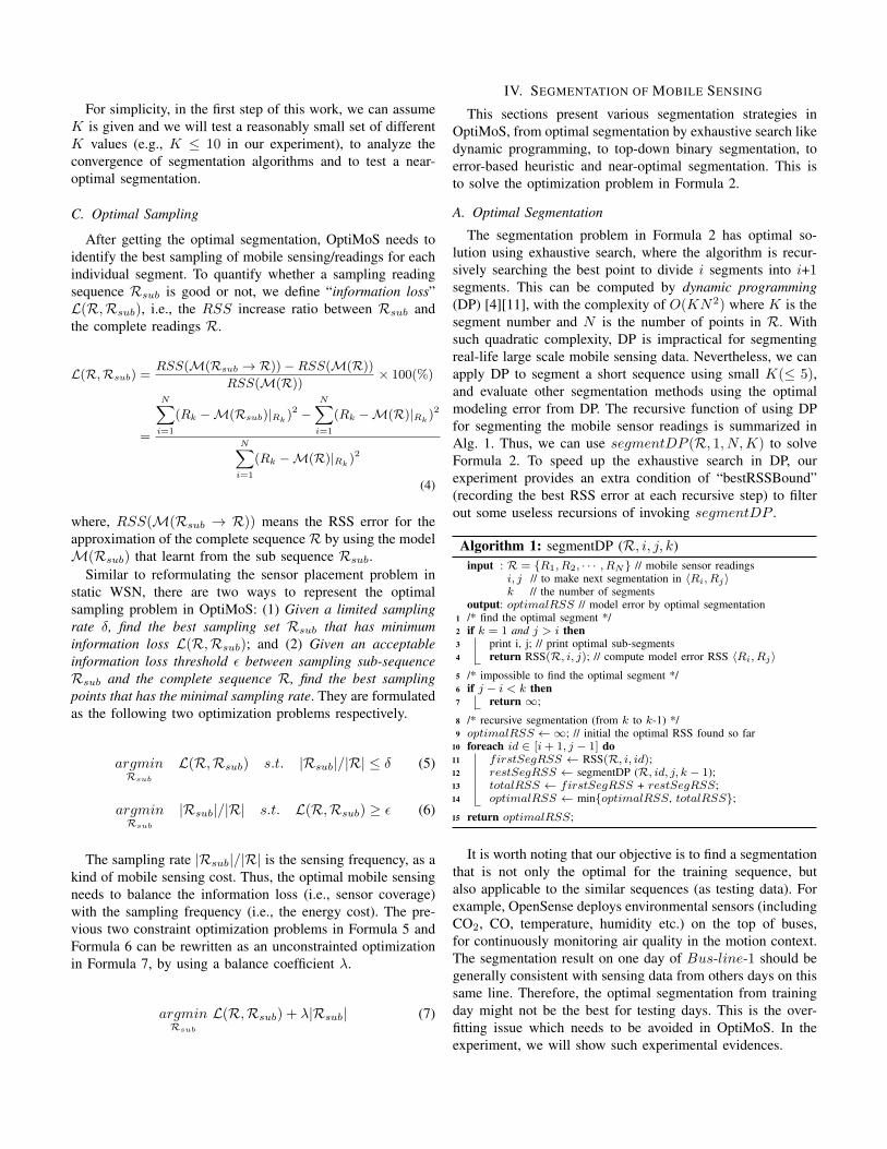
A. Optimal SegmentationThe segmentation problem in Formula 2 has optimal so-

lution using exhaustive search, where the algorithm is recur-sively searching the best point to divide i segments into i+1segments. This can be computed by dynamic programming(DP) [4][11], with the complexity of O(KN2) where K is thesegment number and N is the number of points in R. Withsuch quadratic complexity, DP is impractical for segmentingreal-life large scale mobile sensing data. Nevertheless, we canapply DP to segment a short sequence using small K( 5),and evaluate other segmentation methods using the optimalmodeling error from DP. The recursive function of using DPfor segmenting the mobile sensor readings is summarized inAlg. 1. Thus, we can use segmentDP (R, 1, N,K) to solveFormula 2. To speed up the exhaustive search in DP, ourexperiment provides an extra condition of “bestRSSBound”(recording the best RSS error at each recursive step) to filterout some useless recursions of invoking segmentDP .

Algorithm 1: segmentDP (R, i, j, k)input : R = {R1, R2, · · · , RN} // mobile sensor readings

i, j // to make next segmentation in hRi, Rjik // the number of segments

output: optimalRSS // model error by optimal segmentation1 /* find the optimal segment */2 if k = 1 and j > i then3 print i, j; // print optimal sub-segments4 return RSS(R, i, j); // compute model error RSS hRi, Rji5 /* impossible to find the optimal segment */6 if j � i < k then7 return 1;

8 /* recursive segmentation (from k to k-1) */9 optimalRSS 1; // initial the optimal RSS found so far

10 foreach id 2 [i+ 1, j � 1] do11 firstSegRSS RSS(R, i, id);12 restSegRSS segmentDP (R, id, j, k � 1);13 totalRSS firstSegRSS + restSegRSS;14 optimalRSS min{optimalRSS, totalRSS};

15 return optimalRSS;

It is worth noting that our objective is to find a segmentationthat is not only the optimal for the training sequence, butalso applicable to the similar sequences (as testing data). Forexample, OpenSense deploys environmental sensors (includingCO2, CO, temperature, humidity etc.) on the top of buses,for continuously monitoring air quality in the motion context.The segmentation result on one day of Bus-line-1 should begenerally consistent with sensing data from others days on thissame line. Therefore, the optimal segmentation from trainingday might not be the best for testing days. This is the over-fitting issue which needs to be avoided in OptiMoS. In theexperiment, we will show such experimental evidences.

B. Top-down Binary Segmentation

As the optimal segmentation by DP is impractical for real-life long sequence of mobile sensing data because of its highcomplexity, researchers proposed many greedy segmentationmethods, such as the top-down binary split method [13]. Theidea is to hierarchically split the sequence with maximum errorinto two sub-sequences, until the number of segments reachesK. We call this traditional top-down binary segmentationalgorithm as Binary.

In Binary, the algorithm always choose a segment withthe maximum model-based regression error (RSS) to makefurther segmentation, which may cause the division is only inone segment and its subsegments. As a result, the segmentationresult could be totally unbalanced. This is similar to the worstcase of a binary tree, where the tree is completely un-balancedand becomes a linked list. To overcome this problem, wedesign an extended algorithm of Binary, noted as Binary+.

In Binary+, we design a new RSS error measurement thathas two types of penalties to prevent Binary from alwayschoosing the top RSS error: (1) how much error can bereduced after such segmentation; (2) what is the length sizefor the new segments (noted length), as shown in Formula8, where ↵ is the penalty coefficient. The first penalty is toevaluate the new segments in advance; and the second penaltyis to avoid too short segments because of possible outliers.Alg. 2 provides the procedure of the Binary+ algorithm.

newRSS = RSS(M(Rleft)) +RSS(M(Rright))

[RSS = RSS(M(R))� newRSS + ↵⇥ length (8)

Algorithm 2: segmentBinary+ (R,K)input : R = {R1, R2, · · · , RN} // mobile sensor readings

K // the number of segmentsoutput: segOrderQueue // list of segments

1 /* initial the segment result */2 segOrderQueue Ø;3 /* insert the first segment to the sorted queue */4 segOrderQueue.insert(R, 1, N );5 foreach id 2 [2,K] do6 /* retrieve & remove top error segment from the queue */7 topErrorSeg segOrderQueue.poll();8 /* divide the segment into two subsegments */9 S1 (R, topErrorSeg.begin, topErrorSeg.division);

10 S2 (R, topErrorSeg.division, topErrorSeg.end);11 /* add the two new sub segments into two the sorted list*/12 calculate [RSS for S1 and S2;13 segOrderQueue.insert(S1);14 segOrderQueue.insert(S2);15 segOrderQueue.resort(); // resort for next segmentation

16 return segList;

C. Heuristic Segmentation

The Binary and Binary+ methods focus on finding themaximum error segment (either RSS or [RSS) to identify nextsegment to make division; but for the division point in thesegment, they only apply the middle point, which is trivial.Therefore, we additionally design error-based greedy methodsthat use the model residual of each record to identify segment

division. The residual is computed with the Formula 1. Forsuch heuristic method, a simple greedy strategy is using thetop error point as the division point for the segmentation.Recursively, we recompute the new models for new segments,and find the next top error point as the new division point, untilreach K segments. This segmentation is called “Heuristic”.

Similar to Binary that always pick top error segment tomake next segmentation, Heuristic does the same strategythat always picks top error point as division point. Thus, wedesign an extended version called “Heuristic+” that alsouses the penalty function in Formula 8 to avoid that twodivision points are too close, i.e., the segment is too short.In addition, Heuristic+ doesn’t look for the largest error,but for the longest contiguous sequence of error exceeding acertain threshold (e.g. the error median) and then randomlychoose one of its ending. This way it can isolate segmentsthat have a bias in M(R).

The Binary and Binary+ methods study on finding thenext segment and make division; whilst the Heuristic andHeuristic+ methods study on finding the next division pointsto make segmentation. The last segmentation method wepropose in OptiMoS is B+H+ that combines Binary+ andHeuristic+. The idea is to consider both “the maximum errorsegment to build segmentation” but also “the maximum errorpoint to make division”. The combination is done as follows:the segment to divide is chosen by Binary+ and then, insidethis segment, Heuristic+ is applied to find the segmentationpoint. This way we ensure that the segments have a betterdistribution, like in Binary+, but also that the segmentationpoints is put in a region where the current model has itsworst performance and thereby a certain improvement can beexpected.

V. SAMPLING OF MOBILE SENSING

In this section, we study the second tier of OptiMoS, i.e.,data sampling for each segment from the first tier. OptiMoSneeds to balance the sensor coverage (i.e., minimizing mod-eling errors from mobile sensing samples) and the sensingcost (i.e., the size of samples). This is to solve the optimiza-tion problem in Formula 7, balancing the information lossL(R,Rsub) and the sampling cost |Rsub|/|R|.

A. Optimal SamplingThe optimal sensor placement (or sampling) in an arbitrary

sensing field is a NP hard problem [17][20][7]. For a simplifiedproblem with a limited number of mobile sensing points (N ),the optimal sampling at the sampling rate � requires exhaustivesearch amongst all possible subsets of readings. This needsto consider all combination of �N points from the initial Npoints, which has the complexity of O(N �N ) and is still NP-complete. Therefore, we seek to near-optimal greedy solutionsfor optimal sampling in OptiMoS.

B. Distribution based SamplingIntuitive greedy solutions for sampling the mobile sensor

readings for each individual segment are using some statistical

distributions, e.g., uniform and normal. In this paper, weevaluate the uniform sampling and the random sampling.

• Uniform Sampling – To uniformly select the � percentageof mobile reading points in the segment, the algorithmselects the sensing point at each interval �N . We canapply such uniform sampling with �N�1 times, and eachtime has different offset. The final accuracy of uniformsampling is the average of several trials.

• Random Sampling – In this method, we randomly select�N points from the segment, and make certain numberof trials. Similar to uniform sampling, the final accuracyof random sampling is the average of several trials.

C. Entropy based Heuristic SamplingIn distribution based sampling, selecting sensing points

only considers position distribution. Actually for the uniformsampling and the random sampling, each sensing point has thesame chance to be selected. There is no bias in general.

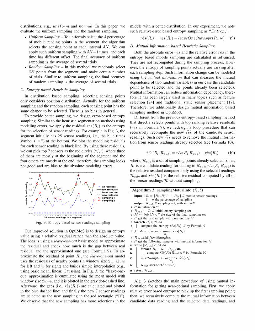
To provide better sampling, we design error-based entropysampling. Similar to the heuristic segmentation methods usingmodeling errors, we apply the residual res(Ri) as the entropyfor the selection of sensor readings. For example in Fig. 3, thesegment initially has 25 sensor readings, i.e., the blue timessymbol (“⇥”) at the bottom. We plot the modeling residualsfor each sensor reading in black line. By using these residuals,we can pick top 7 sensors as the red circles (“�”), where threeof them are mostly at the beginning of the segment and thefour others are mostly at the end; therefore, the sampling looksnot good and are bias to the absolute modeling errors.

1 2 3 4 5 6 7 8 9 10 11 12 13 14 15 16 17 18 19 20 21 22 23 24 25−0.2

−0.1

0

0.1

0.2

0.3

0.4

0.5

25 sensor readings in a segment

resi

dual

for e

ach

read

ing

all readingsraw residualsleave one outnew residulessampling 1sampling 2

Fig. 3: Entropy based sensor readings sampling

Our improved solution in OptiMoS is to design an entropyvalue using a relative residual rather than the absolute value.The idea is using a leave-one-out basic model to approximatethe residual and check how much is the gap between realresidual and the approximated one (see Formula 9). To ap-proximate the residual of point Ri, the leave-one-out modeluses the residuals of nearby points (in window size 2w, i.e. wfor left and w for right) and builds simple interpolation (e.g.,using basic mean, linear, Gaussian). In Fig. 3, the “leave-one-out” approximation is cumulated using the mean model withwindow size 2w=4, and it is plotted in the gray dot-dashed line.Afterward, the gaps (i.e., ˆres(Ri)) are calculated and plottedin the blue dashed line; and finally the new 7 sensor readingsare selected as the new sampling in the red rectangle (“⇤”).We observe that the new sampling has more selections in the

middle with a better distribution. In our experiment, we notesuch relative-error based entropy sampling as “Entropy”.

ˆres(Ri) = res(Ri)� leaveOneOutAppr(Ri, w) (9)

D. Mutual Information based Heuristic SamplingBoth the absolute error res and the relative error ˆres in the

entropy based mobile sampling are calculated in advanced.They are not recomputed during the sampling process. How-ever, the entropy of sampling points actually are varying aftereach sampling step. Such information change can be modeledusing the mutual information that can measure the mutualdependence of two random variables (in our case the candidatepoint to be selected and the points already been selected).Mutual information can reduce information dependency, there-fore it has been largely used in many topics such as featureselection [24] and traditional static sensor placement [17].Therefore, we additionally design mutual information basedsampling method in OptiMoS.

Different from the previous entropy-based sampling methodthat directly selects points with top ranking relative residuals( ˆres in Formula 9), we redesign a loop procedure that canrecursively recompute the new fres of the candidate sensorreadings. Such new fres needs to remove the mutual informa-tion from sensor readings already selected (see Formula 10).

fres(Ri;Rsub) = ˆres(Ri|Rsub)� ˆres(Ri) (10)

where, Rsub is a set of sampling points already selected so far,Ri is a candidate reading for adding to Rsub, ˆres(Ri|Rsub) isthe relative residual computed only using the selected readingsRsub, and ˆres(Ri) is the relative residual computed by all ofthe sensor readings R without sampling.

Algorithm 3: samplingMutualInfo (R, �)input : R = {R1, R2, · · · , RN} // mobile sensor readings

� // the percentage of samplingoutput: Rsub // sampling set, with size �N

1 /* initialization */2 Rsub Ø; // initial empty sampling set3 M int(�N); // the size of the final sampling set4 /* get the first sample with pure entropy */5 foreach Ri 2 R do6 compute the entropy ˆres(Ri); // by Formula 9

7 firstSample argmaxRi

ˆres(Ri)

8 Rsub.add(firstSample);9 /* get the following samples with mutual information */

10 while |Rsub| < M do11 foreach Ri 2 R�Rsub do12 compute fres(Ri;Rsub); // by Formula 10

13 nextSample argmaxRj

fres(Rj)

14 Rsub.add(nextSample);

15 return Rsub;

Alg. 3 sketches the main procedure of using mutual in-formation for getting near-optimal sampling. First, we applyrelative error based entropy to pick up the first sampling point;then, we recursively compute the mutual information betweencandidate data reading and the selected data readings, and

choose the sensing point with the maximum new residual thatremoves the redundancy from existing sampling points. Thisprocedure is stopped until the total sampling rate reaches �.

VI. EXPERIMENTAL EVALUATIONS

This section presents our experimental results of the two-tieroptimal mobile sensing in OptiMoS. We evaluate OptiMos’different segmentation strategies and various sampling meth-ods using real-life environmental data from mobile sensors.

A. Experimental Setup

To evaluate and compare the performances of these algo-rithms, we utilize the real-life mobile sensing data from theenvironmental monitoring project OpenSense [2]. OpenSenseinvestigates informative air quality sensing in terms of de-ploying sensors on top of several public transport vehiclessuch as buses and trams in Switzerland, to achieve a largecoverage of the city area. The longterm objective is to raiseadditional community sensing in the environmental sensingcampaign, using enhanced smartphone/pocket sensors [8] andprivate vehicles [16].

In OpenSense, public transport vehicles are deployed withlocation sensor (GPS) and several environmental measure-ment sensors including temperature, humidity, CO, CO2,NO, NO2, fine particles etc. In current deployment, themeasurement frequency of these mobile sensors are fixed at160Hz, i.e., one sensing record Ri per minute. Fig. 4 showsthe distribution of CO2 measurements from several bus linesin the Lausanne city area during two weeks, where the pointsare the mobile sensing locations and the colors indicates thelevel of CO2 value. This is our early experimental Webinterface for querying and visualizing such mobile sensingdata from the OpenSense project. This Web implementationapplies OpenStreetMap [3] as the embedded map interface.

Fig. 4: Distribution of CO2 measurements from moving buses

To take a concrete look at various mobile sensor measure-ments, Fig. 5 plots one day mobile sensing of several sensorsdeployed on a bus line in Lausanne; the environmental sensorsinclude temperature, humidity, CO, NO2, CO2. From Fig.5, we observe that CO2 has large variance compared to otherenvironmental sensors readings (i.e., CO and NO2). Dueto its large variance for data prediction, modeling on CO2

could be more interesting and challenging; therefore, in ourexperimental study, this paper focuses on investigating theoptimal mobile sensing of the CO2 measurement.

6.6

6.65

6.7

longitude

a)

46.5

46.6 latitude

b)

0

20temperature

c)

40

60humidity

d)

0

2 CO

e)

0

5NO2

f)

00:00 06:00 12:00 18:00 24:00400

450CO2

One day measurement of a bus line (hour)

g)

Fig. 5: One day mobile sensing with various measurements

The mobile sensing objective in OpenSense is to find anoptimal sampling strategy to replace current OpenSense’suniform sampling. This obviously will reduce sensing cost andsave energy. The longterm goal is designing a global optimalsensing for multiple bus lines in the city area, as previouslyshown in Fig. 1 with five bus lines. In this paper, we targetan optimal sensing solution for each individual bus line.

B. Data Model Implementation

There is no model restriction in our two-tier optimal sensingframework. As sketched in Fig. 2 and discussed in Section III,OptiMoS supports all kinds of models such as linear model,polynomial model, SVM regression, time series ARIMAmodel etc. At the moment, our experiments test two types ofmodels, i.e., the basic linear model and the SVM regression.Linear model is simple and efficient to compute; whilst SVMcan achieve high accuracy but requires more computing cost.For SVM implementation, we use the LibSVM package [6],which is largely applied in the literature because of its highcomputing efficiency. All the input data (e.g., CO2 values)were also linearly scaled to [0, 1] for normalization.

0 1 2 3 4 5 6 7 8 9 10 11 12 13 14 15 16 17 18 19 20 21 22 23 24

0.2

0.3

0.4

0.5

0.6

0.7

0.8

One day measurement of a bus line (hour)

Norm

alize

d CO2

Valu

es

Raw CO2 ReadingsLinear RegressionSVM Regression

Fig. 6: Regression for the whole segment

Fig. 6 shows the regression results using the two models(i.e., Linear Regression and SVM Regression) comparedto the raw complete sensor readings at 1

60Hz; this is a 24-hour mobile sensing without any segmentation. By visualcomparison in Fig. 6, the approximation by SVM regression is

close to the ground truth values, which is better than the linearmodel; more precisely, the total model error RSS(M(R))using SVM is 0.0802, whilst RSS(M(R)) from the linearmodel is 0.1004. As shown in Fig. 6, the approximation is notvery good (particularly at the duration of 0am-10am), and wewill show better approximation results by using segment-basedregression in the next subsection.

C. Segmentation ResultsTo evaluate various segmentation methods proposed in

Section IV and make comparison, we define a metric forquantifying the model error reduction by segmentation (fromthe initial non-segment sensor readings R to the K segmentsRi), i.e., the ratio of modeling errors called “RSS Ratio”.

RSS Ratio =

PKi=1(RSS(Ri))

RSS(R)⇥ 100(%) (11)

Fig. 7 presents the RSS Ratio achieved using SVM regres-sion on one-day mobile sensing as the training data. The sixsegmentation methods (i.e., Binary, Binary+, Heuristic,Heuristic+, B+H+, Optimal) are experimented with dif-ferent segment numbers, from 2 to 10. Clearly, with moresegments (i.e., larger K), the error ratio can decrease more.Initially, such error decrease is significant at small K, but laterit becomes more stable when K becomes larger.

Fig. 7: Training on Day-1 by SVM

For individual segmentation methods on the trainingRSS Ratio errors, we observed that the Heuristic+ (orB+H+) method is better than other segmentation methods.We additionally compare them with the optimal solution(Optimal) using dynamic programming when the segmentnumber is small (i.e., K 5). We omit such optimal solutionfor larger K, as the computation time is indeed expensivefor dynamic programming. The RSS Ratio achieved by theHeuristic+ (or B+H+) method is closer to the optimalsolution compared to other methods. Therefore, error-basedheuristic method is good for model-driven segmentation.

To further evaluate the segmentation results learned fromone day training data, we test them on mobile sensing datafrom other days at the same bus line. This test can evaluatethe robustness of our segmentation results. Fig. 8 shows suchtesting errors of RSS Ratio. We observe that Heuristic+

is clearly better than other methods, and even better than the

Optimal for most cases (K = 3, 4, 5). This is the over-fittingproblem, i.e., the optimal segmentation for training data is notnecessarily the best for the testing data.

Fig. 8: Testing on Day-2 using SVM-inferred segments

Fig. 7 and Fig. 8 presented the segmentation results usingthe SVM regression model. For linear regression, we observesimilar trends amongst different segmentation methods. Addi-tionally, the optimal segmentation using linear model in thetraining data works even worse on the testing data. Linearmodel has more prominent over-fitting problems compared tothe SVM modeling. Therefore, in future, we need to furtherstudy more robust optimal segmentation that works not onlyfor training data but also for the test ones.

In contrast to Fig. 6 about regression without segmenta-tion, Fig. 9 shows regression with segmentation (learnt byHeuristic+ when K=5). We observe better regression resultsby using segmentation, particularly at the duration of 0am-10am. In terms of the concrete modeling errors, RSS(M(R))using SVM regression is 0.070 and RSS(M(R)) by linearmodel is 0.081; the two models respectively have model errordecrease 12.7% and 19.3% compared to their modeling errorswithout segmentation shown in Fig. 6. Therefore, segmentationcan gain more error reduction for simpler model (e.g., linear)compared to an advanced one (e.g., SVM).

0 1 2 3 4 5 6 7 8 9 10 11 12 13 14 15 16 17 18 19 20 21 22 23 24

0.2

0.3

0.4

0.5

0.6

0.7

0.8

One day measurement of a bus line (hour)

Norm

aliz

ed C

O2

Valu

e

Raw CO2 ReadingsLinear (5 Segments)SVM (5 Segments)

Fig. 9: Regression in segments (Heuristic+, K = 5)

D. Sampling ResultsTo evaluate different sampling methods that we presented

in Section V, we can use the metric of information loss (seeFormula 4). However, for a very long sequence of mobilesensor readings without segmentation, the information loss can

be negative, as the initial regression on the complete sequencecan be worse than a modeling with a good subsequence ofsampling points. Therefore, we modify the definition of theexact information loss (L) and apply bL(R,Rsub) (i.e., thedirect RSS ratio) to evaluate different sampling methods (seethe following Formula 12).

bL(R,Rsub) = RSS Ratio =RSS(M(Rsub ! R))

RSS(M(R))⇥ 100(%)

=

PNi=1(Rk �M(Rsub)|Rk )

2

PNi=1(Rk �M(R)|Rk )

2(12)

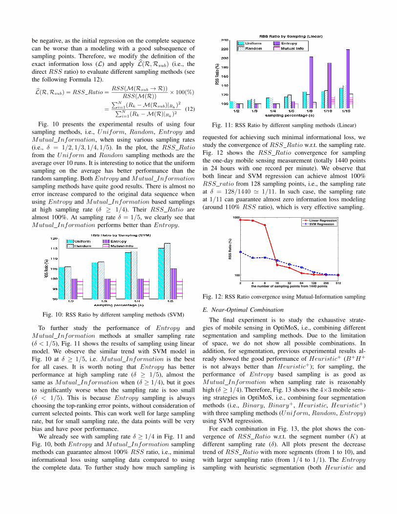
Fig. 10 presents the experimental results of using foursampling methods, i.e., Uniform, Random, Entropy andMutual Information, when using various sampling rates(i.e., � = 1/2, 1/3, 1/4, 1/5). In the plot, the RSS Ratiofrom the Uniform and Random sampling methods are theaverage over 10 runs. It is interesting to notice that the uniformsampling on the average has better performance than therandom sampling. Both Entropy and Mutual Informationsampling methods have quite good results. There is almost noerror increase compared to the original data sequence whenusing Entropy and Mutual Information based samplingsat high sampling rate (� � 1/4). Their RSS Ratio arealmost 100%. At sampling rate � = 1/5, we clearly see thatMutual Information performs better than Entropy.

Fig. 10: RSS Ratio by different sampling methods (SVM)

To further study the performance of Entropy andMutual Information methods at smaller sampling rate(� < 1/5), Fig. 11 shows the results of sampling using linearmodel. We observe the similar trend with SVM model inFig. 10 at � � 1/5, i.e. Mutual Information is the bestfor all cases. It is worth noting that Entropy has betterperformance at high sampling rate (� � 1/5), almost thesame as Mutual Information when (� � 1/4), but it goesto significantly worse when the sampling rate is too small(� < 1/5). This is because Entropy sampling is alwayschoosing the top-ranking error points, without consideration ofcurrent selected points. This can work well for large samplingrate, but for small sampling rate, the data points will be verybias and have poor performance.

We already see with sampling rate � � 1/4 in Fig. 11 andFig. 10, both Entropy and Mutual Information samplingmethods can guarantee almost 100% RSS ratio, i.e., minimalinformational loss using sampling data compared to usingthe complete data. To further study how much sampling is

Fig. 11: RSS Ratio by different sampling methods (Linear)

requested for achieving such minimal informational loss, westudy the convergence of RSS Ratio w.r.t. the sampling rate.Fig. 12 shows the RSS Ratio convergence for samplingthe one-day mobile sensing measurement (totally 1440 pointsin 24 hours with one record per minute). We observe thatboth linear and SVM regression can achieve almost 100%RSS ratio from 128 sampling points, i.e., the sampling rateat � = 128/1440 ' 1/11. In such case, the sampling rateat 1/11 can guarantee almost zero information loss modeling(around 110% RSS ratio), which is very effective sampling.

2 4 8 16 32 64 128 256 512

100

1000

the number of sampling points from 1440 points

RSS

Ratio

(%)

Linear RegressionSVM Regression

Fig. 12: RSS Ratio convergence using Mutual-Information sampling

E. Near-Optimal Combination

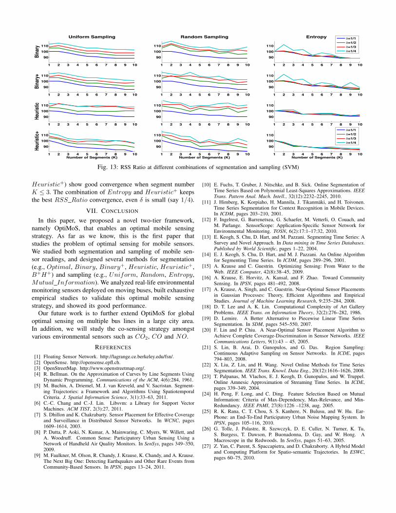
The final experiment is to study the exhaustive strate-gies of mobile sensing in OptiMoS, i.e., combining differentsegmentation and sampling methods. Due to the limitationof space, we do not show all possible combinations. Inaddition, for segmentation, previous experimental results al-ready showed the good performance of Heuristic+ (B+H+

is not always better than Heuristic+); for sampling, theperformance of Entropy based sampling is as good asMutual Information when sampling rate is reasonablyhigh (� � 1/4). Therefore, Fig. 13 shows the 4⇥3 mobile sens-ing strategies in OptiMoS, i.e., combining four segmentationmethods (i.e., Binary, Binary+, Heuristic, Heuristic+)with three sampling methods (Uniform, Random, Entropy)using SVM regression.

For each combination in Fig. 13, the plot shows the con-vergence of RSS Ratio w.r.t. the segment number (K) atdifferent sampling rate (�). All plots present the decreasetrend of RSS Ratio with more segments (from 1 to 10), andwith larger sampling ratio (from 1/4 to 1/1). The Entropysampling with heuristic segmentation (both Heuristic and

1 2 3 4 5 6 7 8 9 10

90100110

Bina

ryUniform Sampling

1 2 3 4 5 6 7 8 9 10

90100110

Random Sampling

1 2 3 4 5 6 7 8 9 10

90100110

Entropy

1 2 3 4 5 6 7 8 9 10

90100110

Bina

ry+

1 2 3 4 5 6 7 8 9 10

90100110

1 2 3 4 5 6 7 8 9 10

90100110

1 2 3 4 5 6 7 8 9 10

90100110

Heur

istic

1 2 3 4 5 6 7 8 9 10

90100110

1 2 3 4 5 6 7 8 9 10

90100110

1 2 3 4 5 6 7 8 9 10

90100110

Heur

istic+

Number of Segments (K)1 2 3 4 5 6 7 8 9 10

90100110

Number of Segments (K)1 2 3 4 5 6 7 8 9 10

90100110

Number of Segments (K)

b=1/1b=1/2b=1/3b=1/4

b=1/1b=1/2b=1/3b=1/4

Fig. 13: RSS Ratio at different combinations of segmentation and sampling (SVM)

Heuristic+) show good convergence when segment numberK 3. The combination of Entropy and Heuristic+ keepsthe best RSS Ratio convergence, even � is small (say 1/4).

VII. CONCLUSION

In this paper, we proposed a novel two-tier framework,namely OptiMoS, that enables an optimal mobile sensingstrategy. As far as we know, this is the first paper thatstudies the problem of optimal sensing for mobile sensors.We studied both segmentation and sampling of mobile sen-sor readings, and designed several methods for segmentation(e.g., Optimal, Binary, Binary+, Heuristic, Heuristic+,B+H+) and sampling (e.g., Uniform, Random, Entropy,Mutual Information). We analyzed real-life environmentalmonitoring sensors deployed on moving buses, built exhaustiveempirical studies to validate this optimal mobile sensingstrategy, and showed its good performance.

Our future work is to further extend OptiMoS for globaloptimal sensing on multiple bus lines in a large city area.In addition, we will study the co-sensing strategy amongstvarious environmental sensors such as CO2, CO and NO.

REFERENCES

[1] Floating Sensor Network. http://lagrange.ce.berkeley.edu/fsn/.[2] OpenSense. http://opensense.epfl.ch.[3] OpenStreetMap. http://www.openstreetmap.org/.[4] R. Bellman. On the Approximation of Curves by Line Segments Using

Dynamic Programming. Communications of the ACM, 4(6):284, 1961.[5] M. Buchin, A. Driemel, M. J. van Kreveld, and V. Sacristan. Segment-

ing Trajectories: a Framework and Algorithms Using SpatiotemporalCriteria. J. Spatial Information Science, 3(1):33–63, 2011.

[6] C.-C. Chang and C.-J. Lin. Libsvm: a Library for Support VectorMachines. ACM TIST, 2(3):27, 2011.

[7] S. Dhillon and K. Chakrabarty. Sensor Placement for Effective Coverageand Surveillance in Distributed Sensor Networks. In WCNC, pages1609–1614, 2003.

[8] P. Dutta, P. Aoki, N. Kumar, A. Mainwaring, C. Myers, W. Willett, andA. Woodruff. Common Sense: Participatory Urban Sensing Using aNetwork of Handheld Air Quality Monitors. In SenSys, pages 349–350,2009.

[9] M. Faulkner, M. Olson, R. Chandy, J. Krause, K. Chandy, and A. Krause.The Next Big One: Detecting Earthquakes and Other Rare Events fromCommunity-Based Sensors. In IPSN, pages 13–24, 2011.

[10] E. Fuchs, T. Gruber, J. Nitschke, and B. Sick. Online Segmentation ofTime Series Based on Polynomial Least-Squares Approximations. IEEETrans. Pattern Anal. Mach. Intell., 32(12):2232–2245, 2010.

[11] J. Himberg, K. Korpiaho, H. Mannila, J. Tikanmaki, and H. Toivonen.Time Series Segmentation for Context Recognition in Mobile Devices.In ICDM, pages 203–210, 2001.

[12] F. Ingelrest, G. Barrenetxea, G. Schaefer, M. Vetterli, O. Couach, andM. Parlange. SensorScope: Application-Specific Sensor Network forEnvironmental Monitoring. TOSN, 6(2):17:1–17:32, 2010.

[13] E. Keogh, S. Chu, D. Hart, and M. Pazzani. Segmenting Time Series: ASurvey and Novel Approach. In Data mining in Time Series Databases.Published by World Scientific, pages 1–22, 2004.

[14] E. J. Keogh, S. Chu, D. Hart, and M. J. Pazzani. An Online Algorithmfor Segmenting Time Series. In ICDM, pages 289–296, 2001.

[15] A. Krause and C. Guestrin. Optimizing Sensing: From Water to theWeb. IEEE Computer, 42(8):38–45, 2009.

[16] A. Krause, E. Horvitz, A. Kansal, and F. Zhao. Toward CommunitySensing. In IPSN, pages 481–492, 2008.

[17] A. Krause, A. Singh, and C. Guestrin. Near-Optimal Sensor Placementsin Gaussian Processes: Theory, Efficient Algorithms and EmpiricalStudies. Journal of Machine Learning Research, 9:235–284, 2008.

[18] D. T. Lee and A. K. Lin. Computational Complexity of Art GalleryProblems. IEEE Trans. on Information Theory, 32(2):276–282, 1986.

[19] D. Lemire. A Better Alternative to Piecewise Linear Time SeriesSegmentation. In SDM, pages 545–550, 2007.

[20] F. Lin and P. Chiu. A Near-Optimal Sensor Placement Algorithm toAchieve Complete Coverage-Discrimination in Sensor Networks. IEEECommunications Letters, 9(1):43 – 45, 2005.

[21] S. Lin, B. Arai, D. Gunopulos, and G. Das. Region Sampling:Continuous Adaptive Sampling on Sensor Networks. In ICDE, pages794–803, 2008.

[22] X. Liu, Z. Lin, and H. Wang. Novel Online Methods for Time SeriesSegmentation. IEEE Trans. Knowl. Data Eng., 20(12):1616–1626, 2008.

[23] T. Palpanas, M. Vlachos, E. J. Keogh, D. Gunopulos, and W. Truppel.Online Amnesic Approximation of Streaming Time Series. In ICDE,pages 339–349, 2004.

[24] H. Peng, F. Long, and C. Ding. Feature Selection Based on MutualInformation: Criteria of Max-Dependency, Max-Relevance, and Min-Redundancy. IEEE PAMI, 27(8):1226 –1238, aug. 2005.

[25] R. K. Rana, C. T. Chou, S. S. Kanhere, N. Bulusu, and W. Hu. Ear-Phone: an End-To-End Participatory Urban Noise Mapping System. InIPSN, pages 105–116, 2010.

[26] G. Tolle, J. Polastre, R. Szewczyk, D. E. Culler, N. Turner, K. Tu,S. Burgess, T. Dawson, P. Buonadonna, D. Gay, and W. Hong. AMacroscope in the Redwoods. In SenSys, pages 51–63, 2005.

[27] Z. Yan, C. Parent, S. Spaccapietra, and D. Chakraborty. A Hybrid Modeland Computing Platform for Spatio-semantic Trajectories. In ESWC,pages 60–75, 2010.