optimizing, testing, and securing mobile cloud computing

Optimizing, Testing, and Securing Mobile Cloud ComputingSystems for Data Aggregation and Processing

Hamilton A. Turner

Dissertation submitted to the Faculty of theVirginia Polytechnic Institute and State University

in partial fulfillment of the requirements for the degree of

Doctor of Philosophyin

Computer Engineering

C. Jules White, ChairJeffrey H. Reed

T. Charles ClancyDouglas Schmidt

Kevin Kochersberger

Nov 20, 2014Blacksburg, Virginia

Keywords: Mobile Cloud Computing, Locational Anonymity, Deployment Optimization,Distributed Smartphone Emulation

Copyright 2014, Hamilton A. Turner

Optimizing, Testing, and Securing Mobile Cloud Computing Systems for DataAggregation and Processing

Hamilton A. Turner

ABSTRACT

Seamless interconnection of smart mobile devices and cloud services is a key goal in modern

mobile computing. Mobile Cloud Computing is the holistic integration of contextually-rich mo-

bile devices with computationally-powerful cloud services to create high value products for end

users, such as Apple’s Siri and Google’s Google Now product. This coupling has enabled new

paradigms and fields of research, such as crowdsourced data collection, and has helped spur sub-

stantial changes in research fields such as vehicular ad hoc networking.

However, the growth of mobile cloud computing has resulted in a number of new challenges, such

as testing large-scale mobile cloud computing systems, and increased the importance of established

challenges, such as ensuring that a user’s privacy is not compromised when interacting with a

location-aware service. Moreover, the concurrent development of the Infrastructure as a Service

paradigm has created inefficiency in how mobile cloud computing systems are executed on cloud

platforms.

To address these gaps in the existing research, this dissertation presents a number of software and

algorithmic solutions to 1) preserve user locational privacy, 2) improve the speed and effectiveness

of deploying and executing mobile cloud computing systems on modern cloud infrastructure, and

3) enable large-scale research on mobile cloud computing systems without requiring substantial

domain expertise.

Contents

1 Introduction . . . . . . . . . . . . . . . . . . . . . . . . . . . . . . . . . . . . . . . . . . . . . . . . . . . . . . . . . . . . . . . . . . . . . . . . . . . . . 1

2 Key Challenges of Mobile Cloud Computing . . . . . . . . . . . . . . . . . . . . . . . . . . . . . . . . . . . . . . . . . 3

2.1 Motivating Scenario . . . . . . . . . . . . . . . . . . . . . . . . . . . . . . . . . . . . . . . 3

2.2 Open Research Problems in Mobile Cloud Computing . . . . . . . . . . . . . . . . 5

2.2.1 Research Gap 1: Locational Data Can Compromise the Anonymity ofMobile Users . . . . . . . . . . . . . . . . . . . . . . . . . . . . . . . . . . . . . . . . 5

2.2.2 Research Gap 2: Predicting and Optimizing Performance of MCC Sys-tems on Modern Cloud Infrastructure . . . . . . . . . . . . . . . . . . . . . . . 7

2.2.3 Research Gap 3: Existing Testbeds are Unsuited to MCC Systems . . . . 9

3 Related Work . . . . . . . . . . . . . . . . . . . . . . . . . . . . . . . . . . . . . . . . . . . . . . . . . . . . . . . . . . . . . . . . . . . . . . . . . . . . 10

3.1 Preserving User Locational Privacy . . . . . . . . . . . . . . . . . . . . . . . . . . . . . 11

3.2 Deploying Mobile Cloud Systems . . . . . . . . . . . . . . . . . . . . . . . . . . . . . . 15

3.3 Large-Scale Mobile Cloud Testing . . . . . . . . . . . . . . . . . . . . . . . . . . . . . 16

3.3.1 Smartphone Testbeds . . . . . . . . . . . . . . . . . . . . . . . . . . . . . . . . . . 16

3.3.2 Related Work in Other Research Domains . . . . . . . . . . . . . . . . . . . . 19

4 Algorithmically Balancing User Anonymity and Data Precision. . . . . . . . . . . . . . . . . . . . . 20

4.1 Overview of Solution Approach to Research Gap 1 . . . . . . . . . . . . . . . . . . 20

4.2 Challenges of Enforcing K-anonymous Tessellation . . . . . . . . . . . . . . . . . . 21

4.2.1 Unknown Data Reading Distribution Makes Region Tessellation Difficult 21

4.2.2 Volatile Data Reading Distribution makes Balancing Privacy and DataPrecision Hard . . . . . . . . . . . . . . . . . . . . . . . . . . . . . . . . . . . . . . . 22

4.3 Research Gap 1 Solution Details: Anonymous Polygon Region Tessellationusing Anonoly . . . . . . . . . . . . . . . . . . . . . . . . . . . . . . . . . . . . . . . . . . . 23

4.3.1 Overview of Anonoly . . . . . . . . . . . . . . . . . . . . . . . . . . . . . . . . . . 23

4.3.2 Model of Anonoly . . . . . . . . . . . . . . . . . . . . . . . . . . . . . . . . . . . . 25

4.3.3 Anonoly Execution . . . . . . . . . . . . . . . . . . . . . . . . . . . . . . . . . . . . 27

4.3.4 Ranking Regions By Resize Priority . . . . . . . . . . . . . . . . . . . . . . . . 29

iii

4.3.5 Reaching Desired Upper and Lower K-bounded Value . . . . . . . . . . . . 29

4.3.6 Merging and Splitting Locational Regions . . . . . . . . . . . . . . . . . . . . 30

4.4 Experimental Results and Validation . . . . . . . . . . . . . . . . . . . . . . . . . . . . 33

4.4.1 Experiment Setup . . . . . . . . . . . . . . . . . . . . . . . . . . . . . . . . . . . . . 34

4.4.2 Experiment Details . . . . . . . . . . . . . . . . . . . . . . . . . . . . . . . . . . . . 34

Comparing Anonoly to Static Tessellation on Real-world Data . . . . . . 34Evaluating Anonoly’s Ability to Maintain Desired K-anonymity Value . . 37

4.5 Contributions and Significance . . . . . . . . . . . . . . . . . . . . . . . . . . . . . . . . 39

5 Quality of Service Aware Optimization of Cloud Resource Allocation . . . . . . . . . . . . . . 42


5.1.1 Using Linux Containers and Strict Resource Limiting To Predict Soft-ware Performance . . . . . . . . . . . . . . . . . . . . . . . . . . . . . . . . . . . . . 42

5.1.2 Using Hybrid Metaheuristic Algorithms to Optimize Software Deploy-ment . . . . . . . . . . . . . . . . . . . . . . . . . . . . . . . . . . . . . . . . . . . . . . 43

5.2 Challenges of Predicting Application QoS Within Multi-tenant IaaS . . . . . . . 44

5.2.1 Relative Resource Limits Make Profiling in Multi-tenant EnvironmentsChallenging . . . . . . . . . . . . . . . . . . . . . . . . . . . . . . . . . . . . . . . . . 45

5.2.2 Splitting Processing Capacity at Granularities Finer Than Single Hard-ware Processors . . . . . . . . . . . . . . . . . . . . . . . . . . . . . . . . . . . . . . 46

5.2.3 Multi-tenancy Introduces Error into Benchmark-based Performance Mod-els . . . . . . . . . . . . . . . . . . . . . . . . . . . . . . . . . . . . . . . . . . . . . . . 46

5.3 Using Hard Resource Limits To Build Effective Prediction Models . . . . . . . 47

5.3.1 Utilizing Hard Limits For Worst-case Benchmarking on Multi-tenantHardware . . . . . . . . . . . . . . . . . . . . . . . . . . . . . . . . . . . . . . . . . . 47

5.3.2 Building Performance Profiles For a Range of Software . . . . . . . . . . . 48

5.4 Experimental Results and Validation For Quality of Service Prediction . . . . . 49

5.4.1 Experimental Platform . . . . . . . . . . . . . . . . . . . . . . . . . . . . . . . . . 49

5.4.2 Dataset and Methodology . . . . . . . . . . . . . . . . . . . . . . . . . . . . . . . 50

5.4.3 Determining Containerization Overhead For a Single Webserver . . . . . 52

5.4.4 Effect of CPU Limiting Mechanisms on Quality of Service . . . . . . . . . 53

5.4.5 Effects of Incorrect Hardware Detection . . . . . . . . . . . . . . . . . . . . . 55

5.5 Validating Performance Models Constructed Using Hard-Limited Linux Con-tainers . . . . . . . . . . . . . . . . . . . . . . . . . . . . . . . . . . . . . . . . . . . . . . . . . 59

5.5.1 Analysis of Experimental Results . . . . . . . . . . . . . . . . . . . . . . . . . . 61

5.6 Contributions and Significance For Quantifying Performance Prediction . . . . 62

iv

5.7 Challenges of Optimizing Task Execution Time on a Multi-core ComputingSystem . . . . . . . . . . . . . . . . . . . . . . . . . . . . . . . . . . . . . . . . . . . . . . . . 65

5.7.1 Complexity of Multi-core Deployment Optimization Necessitates Al-gorithm Scalability . . . . . . . . . . . . . . . . . . . . . . . . . . . . . . . . . . . . 65

5.7.2 Interdependent Constraints Complicate the Use of Heuristics . . . . . . . 66

5.7.3 Comprehensive Testing of An Algorithm for MCDO is Hard . . . . . . . . 66

5.8 Solutions Details for SA+ACO Hybrid Deployment Optimization Algorithm . 67

5.8.1 Mapping Simulated Annealing into Multi-core Deployment Optimization 67

5.8.2 Mapping Ant Colony Optimization into Multi-core Deployment Opti-mization . . . . . . . . . . . . . . . . . . . . . . . . . . . . . . . . . . . . . . . . . . . 69

Pheromone Matrix Representation And Use . . . . . . . . . . . . . . . . 69Pheromone Matrix Updating . . . . . . . . . . . . . . . . . . . . . . . . 71

5.8.3 Integrating SA and ACO Into SA+ACO . . . . . . . . . . . . . . . . . . . . . . 71

5.9 Experimental Results and Validation For Multi-Core Deployment Optimization 72


5.9.2 Comparing To Known Optimal . . . . . . . . . . . . . . . . . . . . . . . . . . . . 74

5.9.3 Runtimes of ACO and SA+ACO . . . . . . . . . . . . . . . . . . . . . . . . . . . 76

5.9.4 Score Comparison of SA+ACO and ACO . . . . . . . . . . . . . . . . . . . . 77

5.10Contributions and Significance . . . . . . . . . . . . . . . . . . . . . . . . . . . . . . . . 80

6 Large-Scale Distributed Smartphone Emulation . . . . . . . . . . . . . . . . . . . . . . . . . . . . . . . . . . . . . . 83


6.2 Challenges of Large-Scale Distributed Smartphone Emulation . . . . . . . . . . . 84

6.2.1 Error-prone, Resource Intensive Agents Increase the Difficulty of Cre-ating Stable Large-Scale Simulations . . . . . . . . . . . . . . . . . . . . . . . . 85

6.2.2 Multiple Software/Hardware Platforms Increase Difficulty of Simulation 85

6.2.3 Large-scale IoT/mobile device Orchestration Requires a Complex In-put Model . . . . . . . . . . . . . . . . . . . . . . . . . . . . . . . . . . . . . . . . . . 86

6.3 Research Gap 3 Solution Details . . . . . . . . . . . . . . . . . . . . . . . . . . . . . . . 87

6.3.1 Architecture of Clasp . . . . . . . . . . . . . . . . . . . . . . . . . . . . . . . . . . 87

HTTP REST Interface . . . . . . . . . . . . . . . . . . . . . . . . . . . 88WebSocket Interface . . . . . . . . . . . . . . . . . . . . . . . . . . . . 89Hybrid Remote API Usage . . . . . . . . . . . . . . . . . . . . . . . . . 91Connecting to TCP services on Worker Nodes . . . . . . . . . . . . . . . 91

6.3.2 Complex, Error-Prone Agents . . . . . . . . . . . . . . . . . . . . . . . . . . . . 92

6.3.3 Providing User Input To Android Emulators Using Clasp . . . . . . . . . . 93

6.3.4 Addressing Failure and Recovery of Smartphone Emulators . . . . . . . . 95

v

6.3.5 Enabling Emulation of Multiple Software/Hardware Platforms . . . . . . 96

6.3.6 Simplifying Simulation Input Model Using Modules . . . . . . . . . . . . . 97

6.4 Experimental Results And Validation . . . . . . . . . . . . . . . . . . . . . . . . . . . . 98


6.4.2 Analysis of Emulator Launch Times and Host Resource Consumption . 99

Node Resources Consumed Per Emulator . . . . . . . . . . . . . . . . . 99Worker Node Degradation When Overloaded . . . . . . . . . . . . . . . 101Emulator Launch Times . . . . . . . . . . . . . . . . . . . . . . . . . . . 102

6.4.3 Emulator Speed . . . . . . . . . . . . . . . . . . . . . . . . . . . . . . . . . . . . . . 103

6.4.4 Task Throughput of Clasp . . . . . . . . . . . . . . . . . . . . . . . . . . . . . . . 105

6.5 Contributions and Significance . . . . . . . . . . . . . . . . . . . . . . . . . . . . . . . . 106

7 Conclusions & Lessons Learned . . . . . . . . . . . . . . . . . . . . . . . . . . . . . . . . . . . . . . . . . . . . . . . . . . . . . . . 107

7.0.1 Summary of Contributions . . . . . . . . . . . . . . . . . . . . . . . . . . . . . . . 107

8 Bibliography . . . . . . . . . . . . . . . . . . . . . . . . . . . . . . . . . . . . . . . . . . . . . . . . . . . . . . . . . . . . . . . . . . . . . . . . . . . . 109

vi

List of Figures

1 Tessellation of the Dartmouth Campus . . . . . . . . . . . . . . . . . . . . . . . . 72 Task Dependency Graph for Program with 9 tasks and 4 Execution Priority Levels . 93 Evolution of Anonoly’s Generated Tessellation Map . . . . . . . . . . . . . . . . . 234 Anonoly vs Static Tessellation Over Two Months . . . . . . . . . . . . . . . . . . 355 Anonoly vs Static Tessellation; Oct 24-Oct 31 Timespan . . . . . . . . . . . . . . 366 Anonoly vs Static Tessellation; Nov 7-Nov14 . . . . . . . . . . . . . . . . . . . . 367 Anonoly vs Static Tessellation; Nov 21-Nov 28 Timespan . . . . . . . . . . . . . . 378 Anonoly vs Static Tessellation Quality of Service; 6 Week Timespan . . . . . . . . 389 Achieved vs Desired K-anonymity; Two Month Timespan . . . . . . . . . . . . . . 3910 Overview of Solution. Inputs are Desired QoS and either Application or Applica-

tion Description, while LXC Soft-Limit Execution Parameters Are Outputs . . . . 4411 Common Resource Consumption Patterns During Testing. (Green, yellow, and red

indicate light warmup, heavy warmup, and benchmarking respectively) . . . . . . . 5112 Average Latency Overhead of Docker Container at Different Concurrency Levels . 5313 OpenResty Performance, Grouped by CPU Limiting Method Used . . . . . . . . . 5514 OpenResty Performance on Percentages of One Hardware Thread . . . . . . . . . 5615 OpenResty Performance, Grouped By Number of Worker Processes . . . . . . . . 5716 OpenResty Average and Maximum Latency, Grouped By Number of Worker Pro-

cesses . . . . . . . . . . . . . . . . . . . . . . . . . . . . . . . . . . . . . . . . . 5817 Performance Prediction Models Versus CPU Constraint . . . . . . . . . . . . . . . 6018 Prediction Error Up To 120 Tenants Per Host . . . . . . . . . . . . . . . . . . . . 6119 Makespans achieved by SA+ACO for different combinations of input parameters.

Each contour line indicates a rise of 0.5 in the log(makespan) . . . . . . . . . . . . 7320 Comparison to known optimal values made by using Equation 10. Thick vertical

lines indicate data median. 1152 samples per Algorithm. . . . . . . . . . . . . . . 7621 Density distribution of runtimes of SA+ACO and ACO. . . . . . . . . . . . . . . . 7722 Percent Change from ACO score to SA+ACO score across the entire range of input

parameters. . . . . . . . . . . . . . . . . . . . . . . . . . . . . . . . . . . . . . . 7823 Enabling Internet Software Integration With Clasp . . . . . . . . . . . . . . . . . . 8824 EmulatorActor Finite State Machine . . . . . . . . . . . . . . . . . . . . . . . . . 9225 Real-time view and control of remotely-hosted mobile device emulators . . . . . . 9426 Node Resources Consumed on Emulator Boot with No Hardware Acceleration . . . 10027 Worker Node Degradation When Launching 80 Emulators with Clasp . . . . . . . 10228 Android 4.0 x86 Emulator Boot Time As a Function of Emulators Already Running

(bars indicate SEM) . . . . . . . . . . . . . . . . . . . . . . . . . . . . . . . . . . 102

vii

29 Timing Common Tasks on Android 4.0 x86 Emulators. Two outliers are not shown:(None,install,15.5 seconds) and (None,keypress,13.5 seconds). . . . . . . . . . . . 104

30 Task Queue Throughput Grouped By Active Emulators . . . . . . . . . . . . . . . 105

viii

List of Tables

1 OpenResty Mean Average and Mean Maximum Latency at 10% CPU, Grouped By

Number of Worker Processes . . . . . . . . . . . . . . . . . . . . . . . . . . . . . 58

2 Comparison of Median Achieved Scores. Task sizes included are [50, 100, 300, 500, 750, 1000]. 76

3 Examples of REST API provided by Clasp . . . . . . . . . . . . . . . . . . . . . . 88

4 Examples of WebSocket publisher-subscriber channels available . . . . . . . . . . 90

ix

1 Introduction

The emergence and subsequent prevalence of smart mobile devices has led to a number of highly

context-aware technologies, such as the Google Now and Siri digital assistants which can monitor

user’s calendar, location, social networks, and other data streams to provide highly-relevant recom-

mendations and information. Simultaneously, purchasing cloud computing services from providers

such as Google (App Engine) and Amazon (Elastic Compute Cloud) has become a mechanism to

reduce capital costs, ensure rapid scalability, and reduce maintenance complexity. Mobile cloud

computing (MCC) studies the integration of these two technologies to enable seamless mergers of

high-power high-context computing, such as real-time recognition of objects or faces in a mobile

device video feed.

While the field of mobile cloud computing has grown rapidly, and multiple systems exist that

utilize both smartphone devices and cloud services, there are nontrivial challenges to continued

growth of mobile cloud computing. An increasingly important concern is the need to balance the

contextual awareness of systems with user expectations of privacy and anonymity. This tradeoff is

complex, as many MCC services provide value through integration of multiple potentially-private

data streams. Removing even one of these streams can drastically reduce MCC service capabilities.

However, attacks exist whereby an attacker can use private information, such as user location,

to derive addition private information, such as health records. Chapter 4 presents Anonoly, an

algorithm to automatically balance the need for highly-accurate location context data with the

desired anonymity of a user.

The growth of mobile cloud computing has also raised a number of questions on effective use of

1

cloud infrastructure. While commercial mobile cloud computing systems require a precise valu-

ation for purchase of services such as cloud infrastructure, multiple challenges currently prevent

simple collection of application performance information. This inability to effectively predict per-

formance is the root challenge for a number of open issues with mobile cloud computing, such

as deploying mobile cloud computing systems onto the cloud for optimal performance, or deter-

mining if the cloud provider is properly delivering purchased hardware. Chapter 5 discusses my

research in modeling quality of service metrics, such as user requests serviced per second, as a

function of cloud infrastructure. Additionally, Chapter 5 discusses my work ensuring that pur-

chased cloud hardware fully utilized, and shows that minor improvements in utilization of each

host can have drastic effects in a service under peak load.

The final challenge addressed in this dissertation is the lack of realistic testing methodologies

for mobile cloud computing architectures. Standard modeling and simulation solutions for test-

ing of large-scale distributed systems do not map well to mobile device testing, due the complex

agents required to emulate mobile devices and the range of mobile operating systems present in

the marketplace. For example, the most widespread major version of Android, Google’s smart-

phone operating system, represents only 36% of the Android ecosystem, with at least seven other

major versions representing significant percentages, and non-Android OSes also present. Chapter

6 presents Clasp, a solution for executing mobile cloud computing system tests involving thou-

sands of mobile devices without requiring intense domain expertise to configure low-level details

of mobile device operating systems.

The remainder of this dissertation is organized as follows: Chapter 2 identifies key gaps in the

existing research and presents a motivational scenario to clarify the current limitations of mobile

2

cloud computing. Chapter 3 provides a comprehensive literature review for each specific challenge.

Chapters 4 through 6 present each solution in detail, including details on the algorithm or software

being presented and empirical validation showing performance compared to prior art. Chapter 7

concludes with a summary of the key research contributions gained from this dissertation.

2 Key Challenges of Mobile Cloud Computing

2.1 Motivating Scenario

The common usage of both mobile computing and cloud computing has created many new op-

portunities and challenges. This section outlines an example scenario which makes the potential

advantages of mobile cloud computing clear, and is loosely based on real-world services [1, 2].

Dexoco, a young mobile development company, chooses to release an Android application that

allows consumers to monitor their mobile carrier’s data network. The application occasionally

samples the mobile data network’s characteristics, such as latency and download bandwidth, and

uses the device GPS to associate the sample with a precise latitude-longitude coordinate. Each

sample is uploaded to the a server program which aggregates samples and generates heat maps to

summarize the performance of the mobile data network in various geographic locations. Dexoco

plans to profit by selling raw data to mobile network operators, who are excited about the vast

array of accurate, real-time data on the health and performance of their network. In order to

make their raw data more desirable, Dexoco collects additional information about user behavior,

such as installed applications and browsing habits. Both Dexoco’s users and the mobile network

3

companies are thrilled with the final product.

However, Dexoco developers quickly realize that selling raw data to the networks will violate

the privacy of their user base. For each data point, Dexoco’s raw data contains fields for the

collection timestamp, user ID (randomly-generated), the GPS location of the data, the network

metrics collected, installed applications and browsing habits. Cellular companies have realized

that their internal logs of which mobile devices connected to which cellular towers allow them

to associate the Dexoco user ID field with their cellular subscriber identity field. The cellular

company can now identify the precise GPS location of their subscribers using the Dexoco data,

as well as associate browsing habits and installed applications with specific customers. Chapter 4

discusses approaches Dexoco can use to ensure customer privacy without sacrificing their business

model.

Dexoco’s next challenges emerge as a result of growth. The increase in users has led to the use of

Amazon’s Elastic Compute Cloud, but the total expense remains high. In addition to traditional

mechanisms of reducing application resource consumption, Dexoco must accurately predict the

tangible benefits of purchasing cloud services and automate the process of purchasing services

during peak hours. New cloud infrastructure models based on Linux containers report substantially

lower costs due to higher hardware sharing, but it is unclear how Dexoco’s software will perform in

this environment. Chapter 5 details solutions to Dexoco’s challenge of cloud resource allocation.

In addition to reducing cost, Dexoco must also ensure their application works properly for all

new users. The Android ecosystem is hugely fragmented, and it is infeasible to purchase all device

models for testing purposes [2]. Standard testing methodologies are incapable of addressing testing

Dexoco’s ecosystem, where large numbers of mobile devices, simulating (or emulating) a large

4

number of different flavors of Android OS, must be simultaneously run the Dexoco application.

Chapter 6 defines solutions for dealing with this challenge, such as constructing mobile device

testbeds that enable this.

2.2 Open Research Problems in Mobile Cloud Computing

This section outlines primary gaps in the research on mobile cloud computing. For each research

gap I discuss the background and current context. While substantial systems have been constructed

using mobile cloud computing technologies, there remain a number of challenges to the next gen-

eration of mobile cloud computing systems. This section outlines the key gaps in existing research.

2.2.1 Research Gap 1: Locational Data Can Compromise the Anonymity of Mobile Users

One major milestone impeding the development of a mobile cloud computing system is the need

to avoid unexpected security and privacy concerns. Mobile operating systems are designed with

features, such as Android’s permission model, to help application developers navigate these con-

siderations. However, there are frequent reports of insecure mobile applications. Similarly, cloud

virtualization technologies such as a hypervisor are designed to isolate customer virtual machines,

yet there are still security issues that prevent businesses from trusting sensitive data in shared-host

environments [3]. In order to avoid substantial legal challenges and to effectively protect valuable

data, creative solutions to the privacy and security challenges of mobile cloud computing environ-

ments have to be created.

One of the largest known risks for mobile cloud computing applications is sensitive data collected

5

via smartphone data collection systems. Smartphone data collection systems are currently used for

a variety of applications, such as health monitoring [4], CO2 emission tracking [5], traffic acci-

dent detection [6], traffic flow measurement [7], and cardiac patient monitoring [8]. Additionally,

multiple middleware layers enable rapid creation and deployment of smartphone data collection

applications [9–12].

Open Problem ⇒ Location Data from Smartphone-powered Data Collection Systems can

be Used to Invade the Personal Privacy of Users. One major challenge of using smartphones

for data collection is the ability to leverage a user’s known location to determine what data was

submitted by a user. For example, in a remote health monitoring system, if each health report

includes the location of the user, then an attacker could follow the user and utilize the user’s

location to determine which health report was his or hers. Conversely, if specific information

about the user is known, such as hair color, eye color, and weight, the attacker could potentially

use this information to filter the data reports and determine the user’s exact latitude and longitude.

While query-based systems, such as location-assisted search, often intentionally provide the user’s

exact location, information gathering applications should be able to operate without compromising

the privacy of the user.

One promising approach of both protecting user’s location data and helping to prevent location data

from being used to identify other private user data is geographical k-anonymity [11]. Geographical

k-anonymity involves making an informed guess regarding the temporal and spatial distribution of

incoming data, and using this assumption to logically break a geographical area into a number

of regions [11] that each contain a minimal number of data readings, as shown in Figure 1. After

sharing this tessellation map with end-user smartphone devices, devices can report regional id’s in-

6

stead of specific latitude/longitude locations. If the real-world incoming data distribution matches

the assumption used to generate the regional tiles, then the incoming data will have the property of

being k-anonymous, where at least k data readings are indistinguishable from one another [11,13].

This ambiguity prevents an attacker from determining users’ exact location or from associating

other private user data using user location.

Tesselation into Regions

Dartmouth Campus Map

23

17

18

12

Initial Data Report Counts

for Region

Individual Users in

Region are Indistinguishable

from Each Other Because

they Only Report Region Identifier

Rather than Lat/Lon Coords

K-Anonymity Value

Determines the Minimum Number of Users

in Each Region that Should be Indistinguishable

from Each Other

Expected Geographic

Distribution of Users and Data

Reports Used to Generate

Tesselation

K1

Region Identifier

Figure 1: Tessellation of the Dartmouth Campus

A good k-anonymity tessellation map is critical for preserving user privacy in a smartphone-

powered data collection system. A key challenge with current tessellation approaches for k-

anonymity is that they use a static, one-time tessellation based on predictions about the data that

will enter the system. If the expected prediction used to generate the tessellation differs too much

from the actual incoming data, the algorithms experience quality of service failures where either

privacy is not preserved, or data precision is reduced needlessly.

2.2.2 Research Gap 2: Predicting and Optimizing Performance of MCC Systems on Mod-

ern Cloud Infrastructure

mobile cloud computing developers have a broad range of hardware packages available for pur-

chase from cloud systems. The offered packages are typically an unmodifiable set of discrete steps,

such as 1024MB of memory and 1.2GHz processor. Deploying software solutions onto this plat-

form is challenging, as a developer must choose which of the configurations will most effectively

7

meet developer goals. This is a complex optimization challenge, and is made much harder due to

the interference effects of other software running on the same hardware, which can cause unex-

pected variance in software performance [14]. Inaccuracies can result in substantial negatives, such

as loss of income or customers. There is therefore substantial interest in precisely understanding

the value of purchasing specific cloud computing services, which is most easily measurable as the

difference in software quality of metrics.

Additionally, cloud providers such as Amazon EC2 use multiple underlying hardware systems to

host virtual machines [14]. These host systems are frequently multi-core systems intended to run

multiple independent workloads simultaneously. However, there are a number of challenges to

effectively utilizing all cores. While software can typically be broken into a number of separate

tasks, there are a number of constraints that make it difficult to determine which tasks should be

executed on which processing cores. One formalization of this is Multi-core Deployment Opti-

mization, or MCDO, which aims to provide a mapping of software tasks onto hardware processors

in such a way that an objective function, typically the makespan or overall execution time of all

jobs, is minimized. In the general case, and even in many cases with relaxed assumptions, obtain-

ing optimal mappings has been shown to be NP-Hard [15, 16]. While substantial research exists

on the MCDO problem, most of the research includes a number of simplifying assumptions that

reduce the usefulness of the final results [17–19].

Open Problem⇒Rapidly Creating Minimal Execution Time Deployments on Heterogeneous

Processors with Communication Costs.

Within the context of MCDO, there has been substantial work on addressing the challenge under

a number of assumptions. These assumptions typically include simplifications such as homoge-

8

neous computing nodes, no communication delays between nodes, or an infinite supply of com-

puting nodes. However, until recently there has been less focus on the more general version of the

challenge, which relaxes the assumptions of homogeneous processors and zero communication

delays. Each software task has pre-established dependencies, as shown in Figure 2, that restrict a

task from running until all of its predecessor tasks have completed. If a task A and its dependency

task A′ are executed on different processing cores P and P ′, then a message must be routed from

P ′ to P upon completion of A′. The time required to route this message is dependent upon the two

processing cores in question, as neighboring cores can communication more quickly than remote

cores. Moreover, each processing core is considered heterogeneous, so some cores will execute

software tasks rapidly while others will execute tasks slowly.

T0

T1 T3

T2

T4 T5

T7

T6

T8

1

22

2

2

3

33

4

Figure 2: Task Dependency Graph for Program with 9 tasks and 4 Execution Priority Levels

2.2.3 Research Gap 3: Existing Testbeds are Unsuited to MCC Systems

The proliferation of mobile smartphone platforms, including Android devices, has triggered a rise

in mobile application development for a diverse set of situations. This in turn has contributed to the

9

rise of mobile cloud computing. Testing of these applications can be exceptionally difficult, due

to the challenges of orchestrating production-scale quantities of smartphones, such as difficulty in

managing thousands of sensory inputs to each individual smartphone device. Moreover, the wide

range of technologies involved in the traditional mobile cloud computing application makes system

testing challenging. Even simple tests require 3-4 different testing frameworks, and isolation of

errors is not at simple as for unit test scenarios.

High profile Android applications such as Facebook have been downloaded by millions of users

[20]. Without a large crowd to test a large-scale application, reliability are performance are difficult

to predict, as shown in a pilot study by Langendoen et al. [21]. Using emulators for application

testing is well-suited for small-scale scenarios, but large-scale emulator orchestration for realistic

network activity simulations is difficult with current technologies.

A number of exploratory frameworks and testbeds for mobile research exist, such as clouds of

physical devices provide interfacing with either personal smartphones or dummy smartphones

[22–24]. However, using personal devices restricts resource and battery consumption, and us-

ing physical devices is expensive and introduces hardware challenges, such as USB interfacing,

when scaling to thousands of devices.

3 Related Work

Mobile Cloud Computing is a relatively young research topic related to both mobile computing and

cloud computing. While some related work specifically targets mobile cloud computing, much of

the relevant literature is organized under the more specific scopes of either mobile computing or

10

cloud computing. This chapter provides a taxonomy of related literature for each of the gaps in

research identified in Chapter 2.2.

3.1 Preserving User Locational Privacy

Multiple methods of preserving user locational privacy in smartphone data collection systems have

been proposed, none of the proposed approaches fully secures the privacy of users. The naive ap-

proach of removing user identifiers from data reports does very little to prevent de-anonymization,

and reports can easily be reassociated with specific users given small amounts of additional in-

formation about the user. Slightly more secure methods require a client to expose sensitive in-

formation to a non-trusted source, such as the server or network peer, which then adds privacy

and anonymity to the data using a more robust method [11, 25–29]. However, requiring sharing

of sensitive data is a key weakness of these methods, and new approaches have been proposed to

reduce data fidelity on a client device, so that no untrusted parties are needed for the data obfus-

cation [30, 31]. However, reducing data fidelity (such as reducing locational accuracy) is not by

itself guaranteed to provide anonymity, and these approaches often create a false sense of security.

For example, generic rules, such as only reporting location to an accuracy of 12mi2, are ineffective

if there are only a few points of interest within each 12mi2 area and the probable location can be

inferred to be a point of interest.

Spatial or temporal blurring reduces the precision of data readings to help ensure the privacy

of the user’s location [32]. For example, users may choose to only report their location to an

accuracy of within 1 mile. Temporal blurring, which is the obfuscation of time, increases the range

of possible time values that a particular data reading may have been generated [33]. There are

11

tradeoffs between the amount of blurring and the usefulness of incoming data. For example, if a

user reports that he is in North America due to spatial blurring, it would be impossible to draw

locational conclusions about users from two different states in the continent, or if a data reading is

timestamped to a day-resolution level, it would be impossible to track change minute-by-minute.

One challenge with spatial and temporal blurring is the difficulty determining how much blurring

is required to ensure anonymity. For example, if there are one-hundred data readings generated

within a five-minute time window originating from within a football stadium, then a good spatial

precision level would be ‘inside football stadium.’ Expanding this example to a continent shows

that the same level of privacy cannot be guaranteed because now specific users can be associated

with specific countries/states (e.g. user X lives in Alaska, and therefore the one data reading from

Alaska is likely from user X).

However, blurring does not guarantee privacy. Entering data reports with very imprecise locations

may seem secure, but there is no guarantee that multiple data reports were entered for each im-

precise location region. An attacker that knows a user’s approximate location when the data was

reported may reassociate that user and their data report with minimal difficulty, because there are

very few reports from that location at that time.

K-anonymity is a method that groups and manipulates data so that ’k’ data items are indistinguish-

able from one another, which solves the issues of simply applying spatial or temporal blurring. This

method is typically applied only after the data has been received, so the system can ensure that there

are at least k-1 data readings in the same locational region [32, 34, 35]. This requires smartphone

users to share their private data with nontrusted sources, who then anonymize the data. By sharing

a tessellation map with end-user devices, Anonoly ensurers k-anonymity without requiring users

12

to share private data.

While the guaranteed anonymity provided by k-anonymity addresses the issues of spatial/temporal

blurring, the method does create some additional challenges. K-anonymity requires non-local

data manipulations that the client must trust when the server performs blurring, which allows

for a possible theft or leakage of private location data. Researchers have attempted to address

the possibility of theft by generating peer-to-peer methods of anonymizing data, but the methods

require a user to trust at least k-1 other users their his/her personal data (and they frequently require

that k-1 users must be online at the time a user wants to submit a data reading) [36, 37].

Region generation is the tessellation of a large area into multiple regions, where each region has an

identifier that is valid to submit to the smartphone data collection system as a localization method

[11]. Predictions about incoming data-report locations and times are used to generate the regions,

and if these predictions match the actual incoming data space/time distribution, then incoming data

reports will be k-anonymous. A key issue is that it is not always possible to predict the location

and time distribution of data readings in advance, and therefore anonymity can be unexpectedly

violated. Moreover, the distribution will likely change over time, rendering the original assumption

incorrect and this method ineffective. Anonoly operates by updating its assumption over time,

thereby reflecting a much closer approximation to the real-world data.

This method is not well suited to scenarios where the distribution of data reading locations and

times vary. In response to a major variance in the data reading locations, the tessellation algorithm

has to regenerate with a new training set of data. For example, Kapadia et al. show that their

method works well from 6:00 - 10:00 PM, but for data reading locations provided before 6:00 PM,

a new tessellation map is needed (assuming that the wireless access point association data looks

13

substantially different from disparate time windows).

While prior work has operated within the assumption that the temporal and spatial distribution of

incoming data readings can be known a priori by using sample data to pre-generate regions, there

are multiple environments where it is impossible or impractical to obtain these early samples.

For example, much of the benefit of smartphone-based data collection systems is the potential

to gather field data from locations where there are not a large number of sensors available. In

a smartphone data collection system for mapping cellular signal strength, the primary benefit of

using smartphones may arise from sensor readings within rural or less populated regions, such as

on hiking trails. However, predictions of the temporal and spatial distribution of incoming data

readings from hikers on various trails is challenging, as there are no available datasets on the

number of hikers that carry their smartphones on such trips.

Range and nearest neighbor queries (NN) are user requests to a location-based service provider

to obtain information about nearby points of interest in a particular category.

Examples of NN queries include: “where is the nearest gas station to my location?” or “what

restaurants are nearby?”. These queries are similar to data collection systems in that the user’s

location information is vital to the relevance of the input data, but differ in that NN queries result

in a response being sent back to the user with the requested information. In contrast, messages

sent to a data collection system do not involve a reply, which creates different privacy needs. For

example, NN queries often include some form of identifier to enable customization of the response

or verification that the user has permission to access the requested data. This results in a range of

privacy challenges and solutions centering around the malicious use of id’s to expose users [38–41],

many of which require users to share their private location data with third parties such as trusted

14

servers or trusted peers.

3.2 Deploying Mobile Cloud Systems

The challenge of optimizing task deployment in a multi-core system, formalized as Multi-core

Deployment Optimization (MCDO), has been extensively studied. Most work in this field contains

a number of simplifying assumptions due to the problem difficulty. For example, [18] does not

consider communication delays between processors. [19] do not consider communication latency’s

caused by limited bus bandwidth. [42] does not consider the general case of MCDO, as the work

focuses on energy usage. An excellent taxonomy of related work in static resource allocation is

presented in [17], including earliest-time-first, modified critical path, and the localized allocation

of static tasks.

Heuristic and Metaheuristic Algorithms Heuristic techniques, such as opportunistic load balanc-

ing [43], are intended to solve problems in a ‘best guess’ manner, and have become increasingly

popular on NP-Complete and NP-Hard problems. Heuristics are often specifically crafted to ad-

dress a single problem type in a specific context. A generalized heuristic technique which makes

very few assumptions about the structure of the problem is termed a metaheuristic. Common meta-

heuristics include simulated annealing, tabu search, ant colony optimization, genetic algorithms,

and others. For the optimization of task scheduling, genetic algorithms in particular have been

used quite heavily as a metaheuristic approach [44].

Approximation Algorithms can be viewed as formally verified heuristics, and have known per-

formance on specific problem types as well as known run-time bounds. Approximation algorithms

15

are popular for guaranteeing a level of confidence in a solution to complex optimization challenges.

3.3 Large-Scale Mobile Cloud Testing

Due to the far-reaching academic and commercial implications of testbeds for production-scale

networks of mobile devices, a range of new research ideas have emerged to enable this. Most

research falls under the taxonomy of smartphone testbeds, which we see as currently composed

of sub-categories for Device Clouds, Participatory Frameworks, and Distributed Emulation. We

first discuss this directly-related area of research, and then briefly summarize work in other fields

that can be applied to the challenges of large-scale smartphone testing.

3.3.1 Smartphone Testbeds

Smartphone testbeds are research solutions directly intended to enable some form of large-scale

experimentation with smartphone devices.

Device Clouds are composed of a number of physical smartphone devices, typically exposed to

experimenters through a web-based interface. This is a variation of traditional clouds of general

purpose computers. For example, the SmartLab is comprised of smartphones connected to a web

interface [24]. SmartLab allows web-based uploading of applications or files, remote shell, re-

booting of devices, etc. The service currently has 40 physical devices online and is available for

researcher use.

Currently, device clouds are limited by the number of devices available and the inherent difficulty

of interconnecting them. Without research enabling physical device sharing, there are concerns

16

about the viability of scaling this approach to networks of thousands of devices.

Participatory Frameworks is a variant of device clouds where the devices used are not purchased

and dedicated to the cloud, but are instead end-user devices connected into the experimentation

suite. End users may either be volunteering or receiving some form of compensation. For example,

PhoneLab by the University of Buffalo [22] is an effort in this area. To initially seed their pool

of devices, they distributed a large number of NSF/Sprint subsidized smartphones to students.

In exchange for use of the smartphone and a free year of cellular services, participants allowed

PhoneLab to 1) track data such as applications used, location, or network signal strength, 2) push

‘experiment’ applications that interact with users.

The Pogo framework [23], based on a similar concept, provides a JavaScript-based interface to

allow non-domain experts to utilize smartphones for research.

While participatory frameworks in some ways solve the cost concerns of device clouds, they are

also limited to small numbers of devices available and the difficulty of interconnecting devices.

They are also restricted to experiments that will not potentially cause harm, such as installing

malware on end-user devices or running software that might break the device.

Distributed Emulation is the process of running a large number of smartphone emulators on

different physical hosts and creating an experimentation environment on top of this distributed

system. Substantial work in this domain has all been performed with the open-source Android OS.

One of the first significant results in this domain was MegaDroid, a 500+ node cluster costing

$500,000 and capable of emulating 300,000 Android emulators [45]. Unfortunately, we could find

no source code or peer-reviewed work explaining how MegaDroid achieves these results. From

17

the limited information available, MegaDroid appears to be using a heavily modified Android

emulator, limited to a single Android version [45], and is currently incapable of allowing fine-

grained control of emulator user input [46].

The next promising results in this domain are Similitude, which focuses on network interconnec-

tion of Android emulators [47]. By using ns-3 to route information between distributed emulators,

and using SimMobility to address time stepping in the distributed environment, Similitude is ca-

pable of simulating multiple types of network environments, such as 3G, LTE, Vehicular Ad-hoc

Networks, etc. However, Similitude requires non-trivial source code modifications to each ap-

plication used, such as replacing the Android LocationManager with Similitude’s own location

provider, and only allows a single version of the Android OS.

Of note is the for-profit service Manymo, which uses distributed emulation to allow developers to

connect to remote Android emulators for faster development [48].

One significant challenge for distributed emulation is the current lack of support for hardware-

assisted virtualization on public cloud providers, such as Amazon EC2. Mobile device emu-

lators perform substantially better and consume fewer resources when capable of utilizing host

hardware directly. Some cloud providers, such as DigitalOcean, have begun to enable hardware-

assisted virtualization within their already-virtualized environments [49]. This hardware-assisted

virtualization-within-virtualization allows a single host to run substantially more emulators than

software-assisted virtualization, and therefore can drastically reduce the cost of large-scale dis-

tributed emulation.

Clasp is a combination of distributed emulation and a device cloud. It is distinct from other

work in that it allows multiple types of Android devices, allows complex dynamic interaction with

18

running emulators.

3.3.2 Related Work in Other Research Domains

This section highlights work from related domains that is relevant to the large-scale distributed

emulation provided by Clasp.

Network and Distributed Agent Testbeds, such as Emulab, PlanetLab, GENI, ns-2, OPNET, and

others provide various mechanisms for experimenting with network protocols or running large-

scale distributed simulations [50–54]. The primary challenge with simulation-based large-scale

smartphone networks is that the programming models of modern smartphone devices are so flexible

that the simulation of each agent becomes very challenging. Different models must be constructed

for each OS type, OS version, Application, Application version, etc. However, there is a large

potential to integrate these systems with distributed emulation smartphone testbeds, such as the

manner used by Similitude [47].

Mobile Systems Testbeds enable experimentation with physical mobile systems (not necessarily

smartphones). One of the largest is the DOME system [55], which covers an area of 150 square

miles and has thousands of access points.

Wireless Sensor Network Testbeds enable experimentation with small mobile devices outfitted

with sensors, typically with considerations such as longevity of battery. MoteLab [56] is a prime

example of this work.

19

4 Algorithmically Balancing User Anonymity and Data Preci-

sion

Both mobile devices and cloud services have substantial privacy and security challenges to over-

come. As referenced in Sections 2.2.1 and 2.1, many mobile cloud computing systems utilize

user’s location. This can cause drastic privacy violations, and new mechanisms to mitigate these

issues are required.

4.1 Overview of Solution Approach to Research Gap 1

To ensure user privacy in smartphone data collection systems, we present a tessellation algorithm,

called Anonoly e.g. ANONymous pOLYgons, that addresses the potential failures present in cur-

rent static tessellation approaches by continually updating the tessellation map based upon in-

coming data. As discussed above, a tessellation map that consistently reflects the real-world can

preserve both user anonymity and data precision. Anonoly is a general solution to creating tes-

sellation maps, which are comprised of regions, where each region is defined as a contiguous

collection of tiles. Tiles, such as small squares or triangles, define the size and shape of the small-

est differentiable unit of real-world geographic data in the tessellation map. Anonoly continuously

samples both the location and the time of incoming data reports, and uses this information to gen-

erate and revise predictions about future incoming data reports’ spatial and temporal distribution.

This dynamic tessellation approach can ensure that both privacy and data precision are consistently

balanced by adapting to changes in the real-world incoming data distribution.

20

4.2 Challenges of Enforcing K-anonymous Tessellation

Current approaches to smartphone data collection frequently report the sensed data, time, and a

precise location where the data was collected. Most methods of anonymizing or increasing the

privacy of data involve reducing the fidelity of that data, which consequently tends to reduce the

usefulness of the data. For example, tessellating a region into polygons of size 10m2 provides more

accurate data about measurements associated with the data report but provides less privacy than

tessellating into regions of 100m2. This section presents the challenges associated with attempting

to enforce k-anonymity across a geographic region.

4.2.1 Unknown Data Reading Distribution Makes Region Tessellation Difficult

A key challenge of tessellating a geographic region to produce k-anonymity is that it requires

knowledge of the temporal and spatial distribution of the future readings from the area. When

the assumed data distribution is incorrect, static tessellation can have two types of quality of ser-

vice failures. First, if the assumption over-estimates the number of incoming data readings, and

generates a tessellation map based on that assumption, then the regions will not receive the min-

imum number of readings required to ensure user locational privacy. Second, if the assumption

under-estimates the number of incoming data readings, then it will generate very large regions in

order to ensure the minimum required number of readings per region is met. This will lead to each

region receiving far more data readings than minimally required, but the locational accuracy of the

incoming data will by much worse than it could have been if the assumption was correct and the

regions were smaller. We term this ‘privacy-induced imprecision,’ whereby the incoming data is

reduced in fidelity in order to protect privacy, but the reduction is over-aggressive and data fidelity

21

(e.g. locational accuracy) is needlessly sacrificed. Static tessellation algorithms can experience

either of the failures if the original assumption about the incoming data distribution was incorrect.

In a smartphone data collection system designed to collect information about cellular signal strength,

the challenge of interest may be generating cellular network coverage maps for remote regions e.g.

on hiking trails, above lakes, etc. In these types of situations, there may be little to zero initial

information about the number of smartphone users that carry their devices into these areas. Addi-

tionally, user smartphone usage habits will likely change in these areas versus more rural locations,

and therefore there is little to no information on how many data readings will be captured. These

unknowns make it difficult to generate an initial assumption about the incoming data spatial and

temporal distribution.

4.2.2 Volatile Data Reading Distribution makes Balancing Privacy and Data Precision Hard

As discussed in Section 4.2.1, a correct assumption regarding the spatial and temporal distribution

of incoming data readings can be used to generate regions that enforce k-anonymity. However,

there is no guarantee that the time and location distribution of incoming data readings will remain

static. The amount of incoming data per region can fluctuate incredibly rapidly, making it very

difficult for the assumption about incoming data to correctly match the real incoming data distribu-

tion. This volatility makes it very difficult to generate a distribution assumption that can constantly

match the real-world distribution. In situations where there are fewer data readings entering the

system than expected (a.k.a the assumption over-estimated), the data reports will not be grouped

with at least k−1 other reports, thereby risking the privacy of users. Conversely, if the assumption

under-estimates the number of incoming data readings, then the tessellation map will have overly

22

large regions (to ensure that each region receives at least k data reports). In this situation, however,

the regions could be smaller without causing any privacy violations, and therefore the locational

imprecision is unnecessary. Balancing the orthogonal desires of privacy and data precision is a

challenging topic.

In a data collection system to collect information on a cellular network, for example, an assumption

might be made that the geographical area of interest will receive at least 200 data readings every

hour, and that assumption used to generate a tessellation map. However, if there are only 50 data

readings being received in one hour, then there will be multiple region identifiers that are used

fewer than the desired k number of times, and the data reports entered into those regions will not

be as private as desired. If the system instead receives 10,000 data readings in one hour, then it is

likely that each region identifier will be used far more than the minimum k number of times. In

this case, it would be possible to use smaller regions, thereby adding better locational granularity

to the dataset, without violating the desired user privacy margin.

4.3 Research Gap 1 Solution Details: Anonymous Polygon Region Tessella-

tion using Anonoly

4.3.1 Overview of Anonoly

Regions in danger of privacy

violation grow in size

Regions that are overly large split

1 Tessellation map

shared with phones

2 Data readings

are input with

region id's

3Data reading counts

used to color

tessellation map4

Retessellation

occurs, new map

shared with phones

5Data readings

are input with

region id's

6New counts are

used to color

tessellation map

Time

Figure 3: Evolution of Anonoly’s Generated Tessellation Map

23

Anonoly is an algorithm for dynamically tessellating a geographic region in order to maintain k-

anonymity, where k-anonymity is a property that has been shown to statistically protect privacy

by making it difficult to associate specific individuals with specific data items [13]. By ensuring

k-anonymity, Anonoly provides a guaranteed level of privacy (e.g. k data reports are indistin-

guishable) which has a number of practical benefits, including removing a potential deterrent for

smartphone users interested in participating in data collection, reducing the severity of system data

leaks, and increasing the potential for commercial datasets to be released for research purposes.

Figure 3 shows how the anonoly algorithm generates and dynamically modifies a tessellation

map of a geographic region in order to protect user privacy. A tessellation map is a set of non-

overlapping polygons with points and edges defined via latitude longitude locations, where the

union of the polygons spans an entire geographical region of interest. The goal of producing the

tessellation map, sharing that map with end-user smartphones, and allowing the smartphones to

enter regional identifiers, is to ensure that user privacy is statically protected by the k-anonymity

property of the polygons.

Counter-clockwise around Figure 3, the following steps are taken:

1. The first tessellation map is sent from server to end-user smartphones. This can either be a

tessellation generated using a priori information about the spatial and temporal distribution

of incoming data readings, or can be a single polygon covering the entire region

2. Smartphones submit data reports, using the downloaded tessellation map to encode precise

latitude longitudes into controlled-precision regional IDs

3. Anonoly, running on the server, sums the number of times each regional ID is used and

24

determines which regions are causing violations.

4. The current tessellation map is improved by increasing the size of regions that received too

few data reports and decreasing the size of regions that received too many data reports.

This improved tessellation map is distributed to end- user smartphones for use in future data

reporting

If the distribution of incoming data is non-volatile, then the tessellation map will converge upon a

map that causes no privacy or imprecision violations. If the distribution of incoming data changes

frequently, then the tessellation map will change rapidly to ensure that the privacy of users is

maintained without significant loss in data precision.

4.3.2 Model of Anonoly

A model of Anonoly is defined for ease of discussion. The model can be described as a 9-tuple:

DAR =< Rs, Tc, K, Cr, Rnk, A, U,M, Sfty, Split, S >

where:

• Rs is a set containing all of the location regions that are currently defined. Each item in Rs

is a closed polygon that defines the outline of one location region

• Tc is the timeslice size, or time between each regeneration of the tessellation

• K is the desired k-anonymity value. For example, a K of 10 would imply that each region

would receive 10 data readings per Tc. If a region receives fewer than 10 readings in Tc, then

25

that region currently invalidates the k-anonymity of the system, and should be increased in

size. If a region receives more than K readings, then that region can potentially be reduced

in size without invalidating k-anonymity, which would improve the locational accuracy of

the incoming data

• Cr is a set of counts that specify the number of data readings that have been input for each

region since the last recalculation. Cr,i indicates the number of data readings input from the

ith region in Rs. After each recalculation, all of the counts in Cr are reset to zero, and Cr is

resized to ensure that |Rs| = |Cr|. Individual data reading counts from Cr are referred to as

C

• Rnk is a function that accepts two regions from Rs and returns an ordering for the two

regions that defines which region is farther from optimal. This allows system administrators

to implement any definition of ‘optimal’ they desire in their system. Multiple possibilities

for Rnk are discussed in 4.3.4

• A is the total area for the environment of interest, in distanceunits2

• U is a function that determines how much a region should grow in response to not meeting

the desired K value. It accepts a region R, and the associated data reading count C for that

region, and returns the amount that the region should grow (in area squared) in response to

the achieved C value

• M is a function that can resize two regions by removing space from one region and allocating

it to another. M is given a region that needs to be resized (the consumer), a value for the

amount of change in area desired (retrieved from U ), and a region that touches the region

26

we are attempting to change (the resource). M will make a best-effort to resize the two

given regions so that the consumer region is given up to the desired amount of area from

the resource region. M will return either a single region that is the full merge of the two

individual regions, or two resized regions

• Sfty is a scaling factor that is multiplied by the desired K value before determining if a

region should be split in response to having an overly large K value. This should never be

below two, as splitting a region that does not have enough incoming data readings to support

2 * the desired K value is likely to result in a privacy violation for one of the descendant

regions

• Split is a function that can determine the number of sub-regions an overly large region should

be split into to meet k-anonymity during the next cycle.

• S is a function that can resize a region by splitting it into multiple sub-regions. The current

implementation splits into similarly sized regions. S is given the region to be resized (the

consumer region) and a value for the desired number of partitions. It will return the generated

set of regions

4.3.3 Anonoly Execution

When the Anonoly algorithm is initially started, Rs is initialized with a single region that encloses

A completely.

For every time range Tc:

1. If there is only one region in Rs, and if the sum of Cr is less than K, then wait one more Tc

27

2. Order all regions in Rs using Rnk

3. Mark all regions as unused

4. While there are unused regions in Rs:

(a) Get the next unused region(R) from Rs

(b) Get the number of data readings(C) that were input into R during this cycle Tc

(c) If C is equal to K, then mark this region as used and continue

(d) If C is less than K, then:

i. Retrieve the amount of desired area change for R from U

ii. Find all the neighboring regions of R that have a C value that is larger than K, and

order them according to Rnk

iii. While R has yet to be changed by the desired area amount (or there are no unused

neighbors), passR, the updated desired area change, and the next-unused neighbor

to M , marking each of the resulting regions as used

(e) If C is greater than K * Sfty, then:

i. Retrieve the number of desired partitions from Split

ii. Pass R and the number of desired partitions to S

iii. Mark all of the returned regions as used and add them to Rs

5. Broadcast updated Rs to all smartphones

If the desired K value is impossible to obtain (e.g. a k-value of 100 is desired, but each time span

Tc only results in 10 data readings), then this initial region will never increase in size.

28

4.3.4 Ranking Regions By Resize Priority

The Rnk function can be implemented in multiple ways, depending upon the needs of the sys-

tem. In general, this ranking algorithm is used to determine which regions are allowed to resize

themselves first. For example, our implementation of Rnk considers privacy violations as being

worse than having far too many data readings for one region. Therefore our implementation, in

attempting to rank regions with a desired k of 10, would consider a region with a k-value of 8 to be

a higher resize priority than a region with a k-value of 2000, even though the latter could clearly

be split into multiple regions and increase location accuracy. We base our priority ranking scheme

upon an implicit assumption that allowing the worst regions first priority in retessellation will result

in a better overall system state. Other approaches for the Rnk function could treat granularity as

more important, or could treat distance from K as the determining factor (thereby sacrificing some

locational privacy for improved granularity). Therefore, Rnk is an effective method of configuring

a privacy vs data granularity system policy.

4.3.5 Reaching Desired Upper and Lower K-bounded Value

The U function of the DAR algorithm, which specifies how much a region should grow in response

to having a smaller-than-desired k-value, can be used to adjust the desired aggressiveness in cor-

recting privacy violations. The U function accepts the actual (i.e. lower than desired) K value and

the current area of a region in Rs, and returns a positive real number that the current area should

be multiplied by to find the total desired area. Overcorrecting a privacy violation by drastically

increasing region size may cause data imprecision violations. Alternatively, failing to adequately

increase region size may result in privacy violations occurring during the next cycle. The same

29

tradeoff applies to the Split function for determining how many sub-regions an overly-large region

is split into. Future work can explore complex variants on the U and Split functions, such as such

as aggressively compensating if a region is small in area and lazily compensating if a region is

large in area.

For our implementation of U , the percent difference between the achieved K and the desired K,

e.g. real/desired, is added to 1 (the current area) and returned to M (described below) to increase

the region size. We intend this approach to be a moderate response to privacy violations, although

future work is needed to determine effective implementations of each subfunction, such as U . The

Split function is given the achieved K value as input, and outputs the number of equally-sized

partitions that this region should be split into. It is known that (in general) we do not wish to

split regions that have less than 2 ∗K values, because it is likely that one of the child regions will

have a privacy violation. We empirically determined 3 ∗ K to be a good split value. Our Split

implementation therefore returns b achievedKdesiredK∗3c.

4.3.6 Merging and Splitting Locational Regions

The M and S functions, respectively, are used to merge and split regions in Rs. These functions

are domain-specific functions provided by the user. While our initial algorithms do little more than

successfully merge and split polygons, future work can build functions that ensure other properties

of interest. For example, all of the tessellation maps will need to be shipped to smartphones at

some point, so a small filesize or the ability to only ship small pieces of the updated map would

be of interest. This concern could be addressed in the M and S functions by attempting to use

long straight lines for polygon edges whenever possible to reduce the amount of data needed to

30

represent the tessellation map.

For the initial implementation of M and S, we represented the entire geographical region as a grid

of square regions called tiles. Each region R is represented as a contiguous set of square tiles. To

split a region α into two regions, we first create a new region β. Then, an appropriate number of

tiles are consumed from α and given to β. ‘Merging’ is a slight misnomer; in reality, the ‘merging’

region involves consuming area from a neighboring region. Therefore, both splitting and merging

require a method which consumes area (i.e. tiles), and the difference between the two operations

is whether the consumed tiles are placed into a new region or an existing region.

The algorithm for consuming tiles from a region is described below, in listing 1. We first find

the border tiles of this region, which is a simple process of locating all tiles that have at least one

neighbor (out of the eight total) that is not also part of the current region. Next, all border tiles

are ordered by their ‘worth’ as a starting point for a consume operation–ideal starting points are

the leaf border pixels that have only one neighbor tile from the same polygon. If this operation

is a merge, then each possible starting point has to also touch the polygon that will be receiving

the consumed tiles. Using fringe locations as the starting point tends to avoid splitting a region

into two non-contiguous regions. Once the possible starting points have been ordered, we find the

first point that is consumable from this list and use it as the actual starting point of the consume

operation. A tile is considered consumable if removing that tile from this region will not cause this

region to become discontinuous.

Once an ideal starting location is found, we create a list representing tiles that will be consumed

and add the starting tile. We then begin iterating over all tiles in this consume list, checking (for

each tile) the eight neighbors - if any of them are safely consumable then we add them to the list.

31

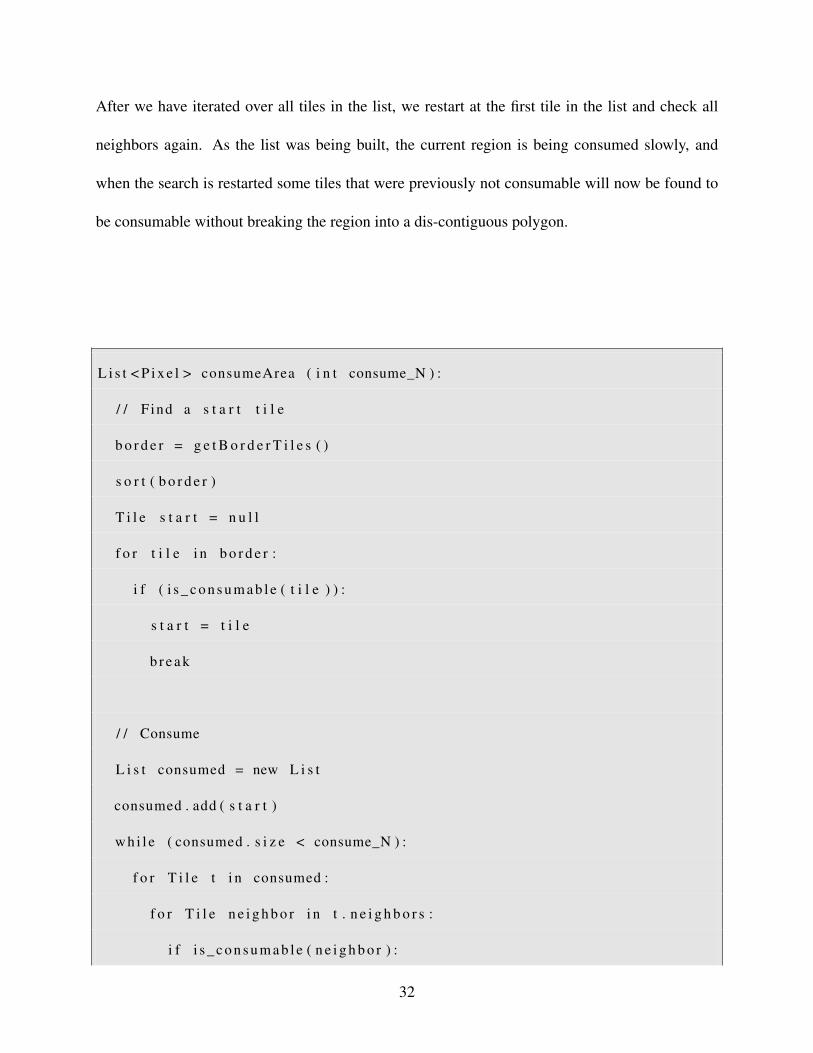
After we have iterated over all tiles in the list, we restart at the first tile in the list and check all

neighbors again. As the list was being built, the current region is being consumed slowly, and

when the search is restarted some tiles that were previously not consumable will now be found to

be consumable without breaking the region into a dis-contiguous polygon.

L i s t < P i x e l > consumeArea ( i n t consume_N ) :

/ / F ind a s t a r t t i l e

b o r d e r = g e t B o r d e r T i l e s ( )

s o r t ( b o r d e r )

T i l e s t a r t = n u l l

f o r t i l e i n b o r d e r :

i f ( i s _ c o n s u m a b l e ( t i l e ) ) :

s t a r t = t i l e

b r e a k

/ / Consume

L i s t consumed = new L i s t

consumed . add ( s t a r t )

w h i l e ( consumed . s i z e < consume_N ) :

f o r T i l e t i n consumed :

f o r T i l e n e i g h b o r i n t . n e i g h b o r s :

i f i s _ c o n s u m a b l e ( n e i g h b o r ) :

32

consumed . add ( n e i g h b o r )

/ / Trim any e x t r a t i l e s

w h i l e ( consumed . s i z e ( ) != consume_N ) :

consumed . remove ( consumed . s i z e − 1)

m y _ t i l e s . removeAl l ( consumed )

r e t u r n consumed

Listing 1: Consuming Area from Region Defined As Grid of Tiles

4.4 Experimental Results and Validation

This section compares the Anonoly algorithm to prior static tessellation approaches using a real-

world dataset obtained from the CRAWDAD.org repository [57]. We ran one experiment to di-

rectly compare Anonoly to static tessellation over the course of a two month timespan by recording

the achieved k-anonymity for both algorithms, and comparing that achieved k-anonymity over the

two month timespan to the desired k-anonymity. Additionally, we ran a second experiment that

compares the ability of Anonoly and static tessellation to balance privacy versus data precision

when the incoming data distribution was undergoing changes.

In order to bootstrap our experiments, we used the CRAWDAD.org dataset to simulate data reports

entering a smartphone data collection system. Each incoming data report must contain a timestamp

and a location (starting as a latitude/longitude on the smartphone device, but converted into a

regional identifier before it reaches Anonoly) in order to be used as input to the Anonoly algorithm.

33

The original dataset is a log of wireless access point associations on the Dartmouth campus, and

therefore we used the time of each access point association, and the latitude/longitude location of

the access point, as the required incoming data. Prior published tessellation algorithms require

manual human intervention to create a tessellation map, and we therefore implemented a static-

tessellation algorithm by running Anonoly for a small time on the dataset and then storing the

generated tessellation for use as a static map.

4.4.1 Experiment Setup

These experiments were conducted on a 2.66 GHz Intel Core i7 MacBook Pro with 4Gb 1067

MHz DDR3 RAM running Mac OS X 10.6.7 and Java SE Runtime 1.6.0_24.

4.4.2 Experiment Details

Comparing Anonoly to Static Tessellation on Real-world Data In this experiment, we gener-

ated a tessellation map and then statically utilized that single tessellation map for the entire dura-

tion of data collection. On the same data, we also utilized the Anonoly algorithm to dynamically

re-tessellate, allowing comparison of the Anonoly algorithm to a static tessellation algorithm.

The Anonoly algorithm will avoid or mitigate the quality of service failures which cause static

tessellation algorithms to be ineffective. Our two predictions regarding how static tessellation

algorithms could potentially under perform are discussed in sections 4.2.1 and 4.2.2.

Experiment Results. Figure 4 shows the k-anonymity which was achieved by a static tessellation

algorithm and the Anonoly algorithm over the course of two months. Each datapoint is the median

34

of the k-anonymity values achieved for all regions during that timeslice. The optimal values for

k-anonymity are located between the blue privacy violation region, and the red privacy-induced im-

precision region. By allowing the k-anonymity value to drop below the set k-anonymity algorithm

parameter of fifteen into the blue privacy violation region, the privacy of users in the smartphone

data collection system is no longer statistically protected. K-values above the safety margin of

forty-five (e.g. in the red zone) indicate that the tessellation could be composed of smaller regions

without causing a privacy violation, and therefore the precision of the locational data could be

improved with no adverse affects. The safety margin of 45 is 3x the privacy margin of 15 - having

a safety margin of 2x is not recommended, as a split will likely cause one of the regions to drop

below 15.

Privacy-Induced

Imprecision

(higher is worse)OptimalPrivacy Violation

(lower is worse)

Figure 4: Anonoly vs Static Tessellation Over Two Months

In order to better understand the results shown in Figure 4, we analyze the data on a week-by-week

basis. The first week, shown in Figure 5, shows Anonoly initially mirroring the static tessella-

tion algorithm results, but the algorithms begin to differ as Anonoly updates its assumptions about

the incoming data distribution. For this experiment, Anonoly was tuned to resolve privacy viola-

tions with moderate adjustments to the tessellation. When violations are detected, Anonoly makes

adjustments to enable the desired level of privacy while also attempting to provide the greatest ge-

35

ographical precision for data reports. However, near the 10-26 datapoint Anonoly reacts to a slight

drop in the median k-value and corrects too aggressively, reaching into the non-desirable privacy-

induced imprecision region. However, the height of Anonoly’s over-correction is still significantly

lower than the height of the static algorithm’s imprecision on 10-27.

Static Algorithm Sacrifices More Data Precision

Figure 5: Anonoly vs Static Tessellation; Oct 24-Oct 31 Timespan

On the third week of data (shown in 6) the difference between the static algorithm and Anonoly

become more significant. There are multiple k-value peaks in the static algorithm where the re-

gions in the tessellation are larger than is required to ensure user privacy. However, the Anonoly

algorithm is able to effectively avoid sacrificing data precision needlessly, and generates a finer

tessellation map as the number of incoming data readings increases, thereby gaining data precision

while safely maintaining the required level of data privacy.

Static Algorithm Sacrifices Data Precision

Figure 6: Anonoly vs Static Tessellation; Nov 7-Nov14

On the fifth week of the dataset (shown in 7), the first privacy violations occur. In the hours

36

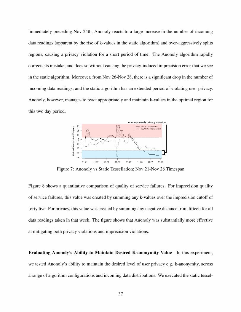
immediately preceding Nov 24th, Anonoly reacts to a large increase in the number of incoming

data readings (apparent by the rise of k-values in the static algorithm) and over-aggressively splits

regions, causing a privacy violation for a short period of time. The Anonoly algorithm rapidly

corrects its mistake, and does so without causing the privacy-induced imprecision error that we see

in the static algorithm. Moreover, from Nov 26-Nov 28, there is a significant drop in the number of

incoming data readings, and the static algorithm has an extended period of violating user privacy.

Anonoly, however, manages to react appropriately and maintain k-values in the optimal region for

this two day period.

Anonoly avoids privacy violation

Figure 7: Anonoly vs Static Tessellation; Nov 21-Nov 28 Timespan

Figure 8 shows a quantitative comparison of quality of service failures. For imprecision quality

of service failures, this value was created by summing any k-values over the imprecision cutoff of

forty five. For privacy, this value was created by summing any negative distance from fifteen for all

data readings taken in that week. The figure shows that Anonoly was substantially more effective

at mitigating both privacy violations and imprecision violations.

Evaluating Anonoly’s Ability to Maintain Desired K-anonymity Value In this experiment,

we tested Anonoly’s ability to maintain the desired level of user privacy e.g. k-anonymity, across

a range of algorithm configurations and incoming data distributions. We executed the static tessel-

37

Higher ValuesAre Worse

Anonoly Privacy

Anonoly excels at avoiding bothprivacy and imprecision

failures

Static Imprecision

Anonoly ImprecisionStatic Privacy

Figure 8: Anonoly vs Static Tessellation Quality of Service; 6 Week Timespan

lation, and the Anonoly algorithm, on a two month section of the CRAWDAD.org dataset, setting

multiple desired k-anonymity values and using multiple timeslice sizes. Our aim in this exper-

iment was to extend Experiment 1, which showed us that Anonoly could avoid privacy-induced

imprecision and privacy violations, to also show that Anonoly can avoid these quality of service

failures while also maintaining the desired k-anonymity value.

The Anonoly algorithm will have k-values closer to the desired k-anonymity than static tessel-

lation’s generated k-values. We hypothesized the Anonoly algorithm would enforce k-anonymity

as well or better than static tessellation methods. Due to Section 4.4.2 showing that Anonoly is able

to successfully avoid or mitigate the two quality of service failures discussed in sections 4.2.1 and

4.2.2, we additionally hypothesize that Anonoly will be able to more effectively maintain a desired

k-anonymity value, even with a wide range of algorithm parameters and different incoming data

distributions.

Experiment Results. Figure 9 shows k-anonymity values generated by the Anonoly algorithm

and a static tessellation. Multiple desired k-values are considered on the x-axis, and the actual

achieved values are plotted on the y-scale. Each point represents the median of the k-values,

error bars represent the 5-95th quantiles. Each algorithm (static and Anonoly) was evaluated with

three different timeslices for each desired k-value, and all achieved k-values were merged before

38

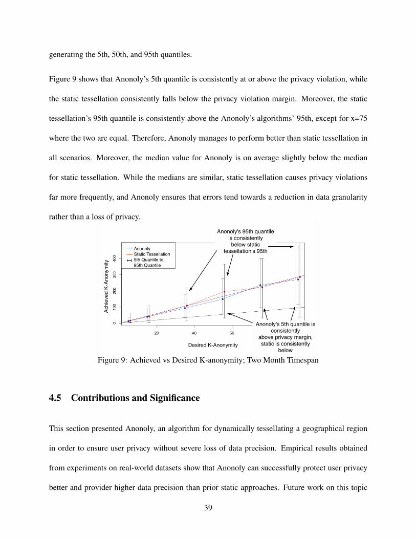
generating the 5th, 50th, and 95th quantiles.

Figure 9 shows that Anonoly’s 5th quantile is consistently at or above the privacy violation, while

the static tessellation consistently falls below the privacy violation margin. Moreover, the static

tessellation’s 95th quantile is consistently above the Anonoly’s algorithms’ 95th, except for x=75

where the two are equal. Therefore, Anonoly manages to perform better than static tessellation in

all scenarios. Moreover, the median value for Anonoly is on average slightly below the median

for static tessellation. While the medians are similar, static tessellation causes privacy violations

far more frequently, and Anonoly ensures that errors tend towards a reduction in data granularity

rather than a loss of privacy.

Desired K-Anonymity

Ach

ieve

d K

-An

on

ym

ity

Anonoly

Static Tessellation

5th Quantile to

95th Quantile

Anonoly's 5th quantile is consistently

above privacy margin, static is consistently

below

Anonoly's 95th quantile is consistently below static

tessellation's 95th

Figure 9: Achieved vs Desired K-anonymity; Two Month Timespan

4.5 Contributions and Significance

This section presented Anonoly, an algorithm for dynamically tessellating a geographical region

in order to ensure user privacy without severe loss of data precision. Empirical results obtained

from experiments on real-world datasets show that Anonoly can successfully protect user privacy

better and provider higher data precision than prior static approaches. Future work on this topic

39

will involve implementing the Anonoly algorithm on a testbed environment with thousands of

smartphone emulator instances, allowing our team to address issues which arise in production

environments, such as data inconsistency, network overheads, and computational cost.

From our research on this topic, we learned the following important lessons:

1. Maintaining k-anonymity on highly-volatile data is possible by updating predictions

about the incoming data distribution frequently. Our research shows that it is quite pos-

sible to maintain the desired privacy in many real-world situations. By testing on a large

real-world dataset, we have shown that it is full reasonable to attempt to build a k-anonymity

algorithm intended to run for multiple years with no modifications. While it is necessary

to predict the distribution of incoming data, we have shown that updating this prediction

frequently is an effective method of dealing with highly-volatile incoming data.

2. Data precision does not necessarily have to be sacrificed to achieve user privacy. As

Section 4.4 shows, there is a direct tradeoff between the precision of incoming data and

user privacy. Prior work, due to an inability to reevaluate assumptions about the incoming

data, typically made decisions to ensure privacy was maintained during worst-case situations.

However, this results in poor data precision in the average case, as precision was consistently

reduced in order to ensure privacy even in non non worst-case situations. Our work has

shown that reevaluation of data assumptions allows much higher data precision in the average

case, while still maintaining privacy in the worst-case.

3. Multiple data types reveal user location. While we have proposed a solution for protecting

user locational privacy, other data included in a data report can easily remove this protection.

40

For example, if a user submits an image that happens to contain part of their vehicle, then

that data report could be linked to that specific user by someone who knows what type of

vehicle they drive.

4. Dealing with report caching and user reputation is an open challenge. Many current

smartphone data collection systems cache data reports on smartphone devices while they

are out of internet range, and submit those reports once internet is connected. Additionally,

many systems attempt to track user reputation and build a list of reputable users. Both of

these features are difficult to incorporate into a privacy-enabling algorithm such as Anonoly.

Future work should investigate methods of combining these desired items with user privacy

algorithms.

5. Multiple tradeoffs are available for preserving k-anonymity. To constantly preserve the

desired k-anonymity, there are some tradeoffs required. However, our research has shown

that there are multiple types of data which can be reduced in order to increase privacy. While

we have shown that both locational and temporal accuracy can be reduced in order to increase

privacy, future work will likely show that there are other components which can be used to

increase system privacy.

The Anonoly algorithm implementation, experiments, and data described in this section are avail-

able in open source form from https://github.com/VT-Magnum-Research/anonoly.

41

5 Quality of Service Aware Optimization of Cloud Resource

Allocation


We propose, develop, and validate two complimentary research solutions for improving Quality

of Service-aware optimization of cloud resource allocations. First, by using Linux Containers and

strict resource limiting we build accurate models of software performance as a function of avail-

able cloud resources. Second, utilization of metaheuristic hybrid algorithms to improving current

mechanisms for deploying software components onto cloud resources. Specifically, methods are

needed to rapidly determine a good placement of software tasks onto cloud resource.

5.1.1 Using Linux Containers and Strict Resource Limiting To Predict Software Perfor-

mance

By utilizing the hard resource limiting features available to Linux Containers, we are able to gener-

ate accurate worst-case performance models for each application by simulating a range of resource

configurations across an extensive array (> 200) of open source web server implementations. We

are also able to investigate the overhead of the different CPU limiting features available to Linux

Containers, and empirically determine which methods have the least overhead when host hardware

is highly shared. Taken together, these two results allow consumers to effectively determine appli-

cation performance on an LXC IaaS cloud, and allow cloud providers to determine which resource

limit methods are effective for high tenancy levels. We conclude with a set of empirically backed

42

recommendations on how to architect an LXC-based IaaS cloud to effective support high-tenancy

conditions such as 100 containers per host.

In Section 5.4 we present empirical data that we have gathered showing that web server perfor-

mance can be accurately predicted across a range of LXC resource limitation levels. We specifi-

cally focus on the methods for effectively scaling the processing capacity a web server is allowed,

and demonstrate that these limitations results in a stable degradation from full performance to

fractions of full performance. Section 5.4 also explores the two main LXC CPU limiting mech-

anisms currently available in the Linux Kernel, CPU pinning and CPU bandwidth limiting, and

presents data indicating that the least wasteful method of achieving large-scale multi-tenant LXC

environments is through a combination of the two methods.

5.1.2 Using Hybrid Metaheuristic Algorithms to Optimize Software Deployment

To address the Multi-core Deployment Optimization problem, we have implemented a hybrid

metaheuristic algorithm that searches for a mapping of tasks onto processors which results in a

minimal makespan. The algorithm continues work in the area of using Ant Colony Optimization

(ACO) to solve the MCDO, but differs from prior work in that it combines an ACO with a Simu-

lated Annealing (SA) algorithm. As shown in Section 5.9, the hybridized SA+ACO algorithm not

only showed an average improvement over the non-hybrid ACO algorithm across a broad range

of inputs, it also showed a large decrease in running time. SA has similar properties to Genetic

Algorithms, such as good handling of nonlinear state spaces, but has been studied substantially

less in the context of MCDO.

43

CPU

RAMIO

Resource Steps

Hard-Limit Benchmark

CPU

Rps

PerformanceModel CPU: 0-11

CFS: 200ms

Soft-LimitExecution

CPU RAM IO RPS Lat100 128 1000 155 2.3500 1024 1000 83 2.520 64 1000 170 2.1720 64 1000 22 2.3300 128 1000 234 2.3450 128 1000 23 2.3210 128 1000 45 2.320 32 1000 56 2.5750 2048 1000 565 2.1

Pre-Generated Performance Models

Application

ApplicationDescription

DesiredQoS

Figure 10: Overview of Solution. Inputs are Desired QoS and either Application or ApplicationDescription, while LXC Soft-Limit Execution Parameters Are Outputs

5.2 Challenges of Predicting Application QoS Within Multi-tenant IaaS

Accurate prediction of application quality of service would save huge amounts of money for cloud

users, but is difficult to accomplish. Issues such as multi-tenancy and soft resource limits compli-

cate the challenge of generating usable data when running on an IaaS cloud.

Traditional models of application performance profiling, as shown in Equation 1, focus on one

metric of software execution such as total runtime Tp, as calculated using the frequency of software

execution Hi and the runtime of individual software blocks Ti:

Tp =n∑i=1

Ti ∗Hi (1)

By expanding this model to include summary statistics for any software metrics providing benefit

~B, such as latency Γ and throughput ∆, we can more appropriately quantify the performance of

software in a cloud environment.

~B =< maxi∈n{Γi ∗Hi},

n∑i=1

Ti ∗Hi,mini∈n{∆i ∗Hi} > (2)

44

The challenge can then be formalized as a solution to Equation 3, where an application A under

a set of constraints ~C on hardware resources such as CPU, RAM, Disk Input/Output, Network

Throughput, etc, can expect at least a minimum of ~B benefit.

f(~C,A) = min ~B (3)

As shown in Section 5.3, our final solution takes the form shown in Equation 4 whereby the so-

lution to Equation 3 can be approximated by providing a high-level description of the application

AD using features such as application programming language, application framework, application

database, etc, and a database E of existing solutions to f(~C,A).

f(AD, ~C,E) ≈ f(~C,A), f(~C,A) = min ~B (4)

5.2.1 Relative Resource Limits Make Profiling in Multi-tenant Environments Challenging

Cloud IaaS providers such as Amazon traditionally use relative, or soft, resource limits that allow a

VM to consume additional resources beyond it’s minimum allowance if those resources are unused

by other tenants. As the Cloud IaaS provider cannot recycle unused computation time, the common

practice is to allow unused computation time to be consumed by the tenants executing on a host.

This is directly relatable to systems such as the Linux Completely Fair Scheduler (CFS), which will

share any unused cycles between processes currently awaiting computation. This creates a substan-

tial burden for performance profiling, as it becomes unclear if benchmark results include any extra

compute time that was unused by other tenants. Moreover, this added uncertainty increases the dif-

45

ficulty of identifying different categories of error present when benchmarking repeatedly, thereby

making it difficult to isolate and eliminate causes of benchmarking noise. For example, it has been

shown that identically specified VMs already have multiple sources of variability [14].

5.2.2 Splitting Processing Capacity at Granularities Finer Than Single Hardware Proces-

sors

An emergent challenge of LXC IaaS is the need to fairly share a host computer amongst a num-

ber of tenants likely exceeding the number of available hardware threads. Traditional mechanisms

for fairly sharing available processor capacity in IaaS focused on variations of CPU pinning (also

known as processor affinity), whereby a process or group of processes is executed solely on des-

ignated hardware processors. CPU pinning is highly effective because 1) processor caches are

more effective when processes execute on the same CPU, and 2) CPU pinning does not require

global process usage counters and therefore requires no coordination between different processors.

However, the unit of division used in CPU pinning is always a single hardware processor, such as

a core or hardware thread, and therefore CPU pinning cannot guarantee equal sharing of multiple

processes executing on the same hardware processor.

5.2.3 Multi-tenancy Introduces Error into Benchmark-based Performance Models

Multi-tenant host systems are inherently challenging to collect benchmark data from, as there is

a clear potential for interference. Amazon EC2 currently shares each physical machine with up

to eight guest VMs. While resource limits exist to fairly subdivide the host machine, prior work

has shown that these resource limits are not enforced with absolute strictness, which can result in

46

worse benchmark results if a neighbor is being noisy. Section 5.3 describes how we address this

challenge by using compute time bandwidth limits of the Linux Kernel.

5.3 Using Hard Resource Limits To Build Effective Prediction Models

As discussed in Section 5.2, detailed models of guaranteed application performance at various

resource allocation levels would enable rapid and accurate deployment of software onto hosts.

By addressing the challenges laid out in Section 5.2, we first developed a method for generating

accurate performance profiles for HTTP web servers running inside Linux Containers. We then

used a large repository of web server implementations to construct performance profiles for a wide

range of web server implementations, varying in programming language, web server framework,

database ORMs, and other factors.

As shown in Figure 10, web application developers input their desired quality of service and either

a description of the application or the application itself. The method will report the LXC launch

options the developer should use to achieve the desired QoS metrics. The critical novel component

is hard-limit benchmarking, which provides solutions to multiple discussed challenges.

5.3.1 Utilizing Hard Limits For Worst-case Benchmarking on Multi-tenant Hardware

To address the challenge of relative resource limits discussed in Section 5.2.1, as well as the chal-

lenge of sharing CPUs at high granularity described in Section 5.2.2, we examine the bandwidth

control feature of the Linux Completely Fair Scheduler (CFS) [58]. Traditionally this feature is

used for allocating relative shares of CPU that are then used to calculate percentage of allowed

47

CPU time. However, it is also possible to define hard resource ceiling parameters that allow limit-

ing of a process to a specific amount of CPU time. For example, CFS bandwidth limits can be used

to define a quota that a process is allowed to utilize e.g. 200ms once every period e.g. 500ms.

CFS bandwidth control successfully avoids the problem of relative bandwidth limitations causing

error in benchmark data, as it enables restricting a Linux Container to the worse case scenario

where no additional resource are available. Moreover, this CFS hard limit can presumably be used

in real-time alongside other LXC IaaS tenants that are using the more common relative limiting, as

the only difference in total system state will be that the CFS-limited container no longer consumes

CPU from the pool of unused compute time.

However, there are a number of practical concerns surrounding the use of CFS limits. For example,

CFS requires coordination between processors to determine how much computation time a process

has received, and the overhead of this coordination is unclear at the moment. Turner et al. over

a brief comparison of CFS limits and CPU pinning but leave a number of issues. In Section 5.4

we test a compare CPU pinning and CFS more fully to generate a cleaner understanding of how to

use CPU pinning and CFS limits in tandem [58]. Additionally, CFS quotas explicitly allow over

subscription e.g. sum(Ci) ≥ C. It is therefore necessary to ensure that the host system is not

oversubscribed before assuming that benchmarks occurring within CFS-limited LXC containers

are guaranteed to receive their quota of resources.

5.3.2 Building Performance Profiles For a Range of Software

To address the primary challenge of predicting application performance, we benchmarked > 100

different web server implementations spanning 21 different programming languages. For each

48

implementation we benchmarked a range of CPU and RAM conditions, and used a linear spline

interpolation to translate these fixed data points into a linear surface. Section 5.4 shows empirical

results on the utility of the database generated with this approach. While each server implemen-

tation we used is initially fully-specified, we found mean results for several broad categories (e.g.

programming languages) and created rough models of performance based on minimal informa-

tion about the application. While these rough models have severe loss of accuracy, they also offer

substantially better performance estimates as opposed to having no prior information.

Using high-level information about their application, such as programming language, the developer

can then consult our database to find worst-case performance models for their application. As the

developer specifies more information about their application, such as programming language and

web framework used, we can supply more accurate performance models. If the developer desires

full accuracy, they can utilize the methods derived in this section and Section 5.4 to generate a

model specific to their application.

5.4 Experimental Results and Validation For Quality of Service Prediction

5.4.1 Experimental Platform

We ran our experiments on the Android Tactical Application Assessment & Knowledge (ATAACK)

Cloud [59], which is a hardware platform designed to provide a test bed for cloud–based analysis

of mobile applications. The ATAACK cloud currently uses a 34 node cluster, with each cluster

machine containing Dell PowerEdge M610 blade running Ubuntu 14.04.1 LTS and Linux Kernel

3.13.0-39-generic. Each node has two 12-core Intel Xeon E5645® processors, each with 18GB

49

dedicated DDR3 ECC memory (total of 36GB shared). All nodes were reformatted prior to this

work, and therefore were guaranteed to use the default configuration options of Ubuntu.

For testing LXC we utilized the Docker platform, which provides a number of additional features,

such as automatic build scripts and container versioning, on top of the core Linux Container plat-

form. Each node Docker version 1.14 with the Linux Container execution driver version 1.0.6.

The AUFS storage driver was used to provide container filesystem support.

5.4.2 Dataset and Methodology

To enable data collection across multiple programming languages, web server implementations,

and framework stacks, we used the open source TechEmpower FrameworkBenchmarks (TFB)

project as a core component in our experimentation [60]. For this research, TFB provided auto-

mated installation and load testing for > 100 different web server implementations spanning 21

different programming languages. We provided substantial improvement to the project, such as

the ability to launch web servers inside of Docker containers, and have contributed over 450 git

commits to the main TFB project as well as an additional 150 git commits to our fork of the project

focusing on Linux Container compatibility.

Each framework included in TFB may define multiple tests intended to emulate common aspects

of a real-world web server implementation, such as the speed of common database queries. We

chose to utilize the json test, in which a web server must allocate and serialize a new JSON object

for each request, for most of the experiments shown in this section. This test type exercises the

effectiveness with which a web server can utilize available processor capacity while allocating and

deallocating large numbers of small objects. It also avoids potentially overloading the network

50

capacity of traditional Ethernet network interfaces, which can be a challenge with some of the

other test types defined by TFB.

Each test included a slow warmup, fast warmup, and then the actual benchmarking. During each

test the Linux dstat tool was used to monitor memory, disk, network, processor, and kernel

statistics. Figure 11 shows common patterns of hardware consumption during a test sequence.

10.0

12.5

15.0

17.5

0 25 50 75Time in Seconds

Load

0

10

20

30

40

50


CP

U U

sage

1556

1558

1560

1562

0 25 50 75Time in SecondsC

onsu

med

Mem

ory

(MB

)

200

300

400

500

600


Ope

n S

ocke

ts

Figure 11: Common Resource Consumption Patterns During Testing. (Green, yellow, and redindicate light warmup, heavy warmup, and benchmarking respectively)

Early experiments showed that our networking hardware was restricting performance for high-

performance frameworks, as they were using 100% of our available NIC bandwidth. To address

this issue without dropping these high-performing frameworks, we ran the load generation system

inside a second LXC container on the same host. Load generation was CPU pinned to one proces-

sor and the web server under test was pinned to the second processor, each of which has it’s own

51

memory bank. We validated that non-peak web server performance was not different as a result

of this modification, and were able to successfully continue gathering data to build performance

models beyond our prior peak capacity.

5.4.3 Determining Containerization Overhead For a Single Webserver

The solution approach described in Section 5.3 relies heavily on Linux Containers for isolation of

web applications. With any isolation mechanism, e.g. Virtual Machines, Docker Containers, Linux

Containers, etc, it is critically important to understand the magnitude of resources consumed by the

isolation mechanism. High isolation costs, such as those experienced by Virtual Machines, reduce

the total number of isolated applications that can be deployed onto a single host. While extensive

work has been done to examine the resource consumption of traditional Virtual Machines, few

published works examine the resource consumption of Linux Containers [61].

This experiment compares the performance of running a webserver inside of a Linux Container

versus running in a non-virtualized environment. We expect to see minor performance degradation

due to the isolation overhead.

Experiment Methodology. As web servers are commonly tested using a range of concurrency

levels, we chose to examine overhead individually for six different concurrency levels in order to

capture any differences that might appear between steady-state and heavy-load conditions.

Experiment Results. The results shown in Figure 12 indicate a latency overhead of 10ms when

executing software inside a Docker Container. This is a minor overhead compared to other systems

that enable network isolation, such as the 60ms of a common VM solution [61]. This confirms

52

Figure 12: Average Latency Overhead of Docker Container at Different Concurrency Levels

the work of Felter et al., who are the only other authors we have found to examine the performance

overhead of Docker containers [61].

5.4.4 Effect of CPU Limiting Mechanisms on Quality of Service

When limiting CPU as described in Section 5.3, it is critical to understand the effect the CPU

limiting mechanism has on process performance. To evaluate this effect, we conducted a series of

experiments gathering performance data at various CPU levels using the two most common CPU

limiting mechanisms of CPU pinning and CPU bandwidth control. To understand this effect, we

profiled software performance metrics while limiting software using both methods.

Experiment Results. Figure 13 shows the performance effects of various CPU resource limiting

53

mechanisms. As expected, CPU pinning results in higher throughput for most CPU values, presum-

ably because CPU pinning does not require coordination between different processes. However,

there is an unexpected but repeatable effect of CFS resource limiting outperforming CPU pinning

at 70-80% CPU allowance.

The latency metrics in Figure 13 show that CPU pinning outperforms CFS resource limiting for all

values but the lowest. However, upon careful examination readers may note that CFS was allowed

10% of total available CPU and CPU pinning allowed only 8% of total available CPU. Future

results show that CFS at 8% experiences a similar spike in latency. These low-CPU latency spikes

are a natural result of stress testing at low CPU levels, as the traditional independence of latency

and throughput is removed due to queuing time increases once available CPU is consumed. These

results therefore lead us to conclude that CPU pinning consistent results in lower latency values

than CFS quota limits.

However, CPU pinning is incapable of sharing compute resources finer than a single hardware

processor. Figure 14 shows the effectiveness of CFS quota limits at a granularity lower than a

single core.

There is a clear linear relationship between throughput and CPU for fractions of a processor smaller

than 50%, and steady-state operation from 60% to 100% of the hardware thread. This is consistent

with the measured latency values, which stabilize above 60% allowed.

54

50

100

150

10 20 30 40 50 60 70 80 90 100

K R

eque

sts

/ Sec

ond

CPU Limiting Method

CFS quotas

CPU pinning

0

500

1000

1500

10 20 30 40 50 60 70 80 90 100Percent CPU

Late

ncy

In M

illis

econ

ds

Figure 13: OpenResty Performance, Grouped by CPU Limiting Method Used

5.4.5 Effects of Incorrect Hardware Detection

Many web servers detect available hardware and optimize their startup scripts for performance.

Out of the 120 frameworks that we examined in this work, we found at least 29 that were detect-

ing available hardware and dynamically tuning their startup to maximize performance. The most

common observed optimization was detection of CPU cores, with detection of available RAM be-

ing the next most common. However, fundamental tools used to detect the available resources

such as the Linux free utility, or the Python multiprocessing.cpu_count() method, do

not support Linux containers. These tools report the resources present on the host instead of the

55

0

5

10

15

25 50 75 100

K R

eque

sts/

Sec

ond

10004000

8000

16000

25 50 75 100Percent of Core

Late

ncy

in M

illis

econ

ds

Figure 14: OpenResty Performance on Percentages of One Hardware Thread

resources available for use by the current process.

To understand the negative consequences of this incorrect configuration, we examined the most

common error found - web servers using Nginx as a load balancer between multiple backend

processes often misconfigured the number of Nginx worker processes. According to the documen-

tation the number of workers should equal to the number of hardware processors for maximum

performance. To understand the effects of misconfiguration at various CPU pinning levels, we

benchmarked OpenResty (a Lua web server extending Nginx) across a range of CPU pinning set-

tings with the correct number of workers (e.g. ‘1x’), twice the correct number of workers (e.g.

56

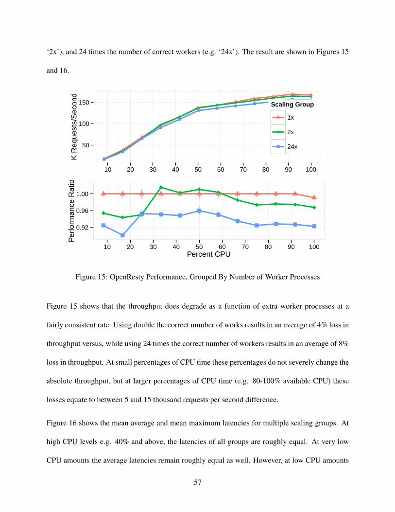
‘2x’), and 24 times the number of correct workers (e.g. ‘24x’). The result are shown in Figures 15

and 16.

50

100

150

10 20 30 40 50 60 70 80 90 100

K R

eque

sts/

Sec

ond

Scaling Group

1x

2x

24x

0.92

0.96

1.00

10 20 30 40 50 60 70 80 90 100Percent CPU

Per

form

ance

Rat

io

Figure 15: OpenResty Performance, Grouped By Number of Worker Processes

Figure 15 shows that the throughput does degrade as a function of extra worker processes at a

fairly consistent rate. Using double the correct number of works results in an average of 4% loss in

throughput versus, while using 24 times the correct number of workers results in an average of 8%

loss in throughput. At small percentages of CPU time these percentages do not severely change the

absolute throughput, but at larger percentages of CPU time (e.g. 80-100% available CPU) these

losses equate to between 5 and 15 thousand requests per second difference.

Figure 16 shows the mean average and mean maximum latencies for multiple scaling groups. At

high CPU levels e.g. 40% and above, the latencies of all groups are roughly equal. At very low

CPU amounts the average latencies remain roughly equal as well. However, at low CPU amounts

57

10

100

1000

10000

10 20 30 40 50 60 70 80 90 100Percent CPU

Late

ncy

In M

illis

econ

dsScaling Group

1x

2x

24x

Figure 16: OpenResty Average and Maximum Latency, Grouped By Number of Worker Processes

the maximum latency is heavily influenced by the degree of misconfiguration, as the 24x scale

group has substantially higher maximum latency than the 1x scale group, as shown by Table 1.

Average MaxScale 1x 1458 1615Scale 2x 1577 2362Scale 24x 6293 25649

Table 1: OpenResty Mean Average and Mean Maximum Latency at 10% CPU, Grouped By Num-ber of Worker Processes

As the target for this research is performance on IaaS host computers with large numbers of tenants,

the most interesting effects occur at small amounts of available CPU e.g. 30% total CPU. At

58

this range, we can conclude that incorrectly detecting available hardware has minimal effects on

throughput, but has potentially substantial effects on maximum latency.

5.5 Validating Performance Models Constructed Using Hard-Limited Linux

Containers

To validate the solution method, we used the proposed method to construct performance models for

120+ web application frameworks. Figure 17 shows a summary of the output performance models,

which predict the minimum guaranteed application quality of service when that application is

executed under the given CPU constraint.

We then used standard soft resource limits to create a Linux-Container based IaaS where each

tenant was given an equal amount of total available CPU. Each tenant was put under the same

stress test that was used to profile it’s performance, with the aim being to determine if the achieved

maximum performance under constraint was equal to the predicted performance under constraint.

Two scenarios were exercised - the first scenario only contained web application frameworks inside

the containers under test, while the second group also include a non-web application container

designed to saturate all available resources and interfere with the running of the web applications

as much as possible. The second group directly simulates the ‘noisy neighbor’ effect of traditional

IaaS performance profiling. If the solution method proposed works perfectly, there will be no

substantial difference in achieved performance under these two scenarios.

To reduce system interference, the cgroup ‘user’ (which contains system tasks such as SSH) was

allocated 1024 shares of CPU time, while the cgroup ‘lxc’, which housed all of our tenants, was

59

0

100

200

300

10 20 30 40 50 60 70 80 90 100Percent CPU

K R

eque

sts/

Sec

ond

Language

C

Go

Java

JavaScript

Lua

Perl

Python

Scala

Ur

Figure 17: Performance Prediction Models Versus CPU Constraint

allowed 65536 shares of CPU time. Each tenant was allowed 1024 shares, and was executed

inside the ‘lxc’ cgroup. The total ‘lxc’ group therefore was guaranteed 6553665536+1024

= 98.5% of the

total CPU time, while each tenant container was guaranteed 1N∗ 98.5 CPU time, where N is the

number of tenants currently executing. For 5 tenants, each tenant container would be guaranteed

15∗ 98.5 = 19.7% of available CPU time.

Figure 18 shows the percent error difference between achieved and predicted performance, where

a result of 0% indicates that the model perfectly predicted the software performance. The two

scenarios are nearly identical, indicating the prediction method is resiliant to the noisy neighbor

60

−4

−3

−2

−1

0

1

1 2 3 4 5 6 7 8 9 10 20 30 40 50 60 70 80 90100120Number of Tenants

Per

cent

age

Err

or

Noisy Neighbor

False

True

Figure 18: Prediction Error Up To 120 Tenants Per Host

effect. Figure Figure 18 also shows that, up to 120 tenants sharing a single physical host, the

maximum percent error is 3%.

5.5.1 Analysis of Experimental Results

The results presented in this section lead to the following conclusions on the effectiveness of shar-

ing hosts among hundreds of tenants and predicting software performance in this environment.

First, we find that using CPU pinning to limit the compute time of a web server results in pre-

61

dictable application performance degradation in the absence of other processes competing for the

designated processors. We also find that CFS quotas allow reasonable segregation of individual

hardware processors, but exhibit sub-par performance when used with multiple physical proces-

sors. In particular, CFS has substantial overhead when used to limit process compute time across

multiple physical processors.

We also found that multiple applications examine available hardware resources, such as avail-

able physical processors, in order to tune their startup parameters. However, most of the methods

used do not properly support LXC resource limits, and therefore report incorrect available hard-

ware. The most common problem we found across the 120 different frameworks examined was

incorrectly detecting available hardware processors, which resulted in up to a 10% decrease in

performance.

5.6 Contributions and Significance For Quantifying Performance Predic-

tion

This research focused on the emerging model of using Linux Containers (LXC) to provide Infras-

tructure as a Service (IaaS) cloud computation. LXC typically has substantially lower resource

overheads than the Virtual Machines (VMs) traditionally used to enable isolation in IaaS environ-

ments, which enables order-of-magnitude increases in the number of tenants that share a physical

IaaS host. However, the overhead and fairness of methods used to fraction a host system into tens

or hundreds of isolated containers are not well understood. Moreover, increases in multi-tenancy

increase the difficulty of predicting application performance inside of the IaaS, as explained in

62

Section 5.2.

To address these challenges, this work develops a method of accurately benchmarking expected

application performance in a multi-tenant LXC-based IaaS. We also investigate the effect that

various resource isolation mechanisms, such as mechanisms to fairly share compute time amongst

tens or hundreds of tenants, have on application performance and quality of service. This work

focuses on the performance of web servers, which is a broad category encompassing a wide range

of the technologies currently used in VM-based IaaS clouds.

This work provides the following contributions and observations regarding appropriate construc-

tion and use of Linux Container-based Infrastructure as a Service Clouds:

1. Combined Use of CPU limiting mechanisms is necessary for effective sharing of host

processors. While CPU pinning is a low-overhead solution for coarse resource limits, CFS

quota management enables fine-grained resource sharing. As described in Section 5.4, an

effective solution is to utilize both mechanisms in tandem.

2. A Method For Predicting Expected Application Performance in a Multi-tenant LXC-

based IaaS, based on utilization of hard resource limitations, is described in Section 5.3 and

validated in Section 5.4.

3. LXC IaaS Providers Should Offer Hard-Limited Containers. As Section 5.4 shows,

strict resource limits mitigate many of the existing challenges of application performance

profiling inside a multi-tenant environment. Additionally, offering isolated environments

with hard limits does not negatively affect other tenants currently executing on a physical

host. We therefore strongly recommend that LXC IaaS systems are architected with perfor-

63

mance profiling, as enabled by hard-resource limits, being a first-class design consideration.

4. Linux Container Overhead Is Negligible For Many Use Cases. As shown in Section 5.4

and corroborated by Felter et al. [61], the overhead of Linux Containers is equal to or less

than the overhead of Virtual Machines for most common metrics. Therefore any software

currently running on a VM-based IaaS cloud can presumably execute on a LXC-based IaaS

cloud at equal or higher levels of performance.

5. Few Resource Detection Tools Support LXC. Most of the resource detection utilities and

functions we encountered across 120 different web frameworks did not support LXC re-

source limiting, and therefore incorrectly estimated available resources by large margins

when executed inside Linux Containers. Existing applications that used these tools com-

monly configured themselves in a suboptimal manner based on these incorrect results.

6. A Large, Diverse Database of Web Server Performance Information is made available

as part of this research. This dataset spans 21 programming languages, 120 web server

frameworks, and over 600 different toolset configurations. Minimally, each test has at least

30 samples of performance statistics, each gathered from 500,000 individual HTTP requests,

and aggregated into the common metrics throughput and latency

The data and experiments described in this chapter are available in open source form from

https://github.com/hamiltont/FrameworkBenchmarks.

64

5.7 Challenges of Optimizing Task Execution Time on a Multi-core Com-

puting System

Effective solutions to the Multi-core Deployment Optimization (MCDO) problem can vastly in-

crease the value of many modern computing systems by increasing the throughput of the hardware

without any physical modifications. With new trends towards massively parallel computer systems,

MCDO is a critical practical issue for obtaining the full potential of these new systems. However,

MCDO has been shown to be NP-hard [15, 62, 63] by multiple researchers. This section outlines

some of the specific challenges encountered while trying to find short runtime, high performance

solution algorithms to the MCDO problem.

5.7.1 Complexity of Multi-core Deployment Optimization Necessitates Algorithm Scalabil-

ity

Multiple works have shown that MCDO is NP-Hard [15, 62, 63]. Unless P = NP , there are no

methods to find an optimal solution to MCDO in polynomial time. While a number of assumptions

can be made to help simplify the challenge, and therefore hopefully reduce the time complexity, a

combination of multiple assumptions must be made to reduce the complexity from NP-hard [62].

Adding these simplifying assumptions reduces the practicality of the final solution. Therefore a

critical challenge is how to find a solution approach that can scale to solving MCDO problem sets

with large numbers of cores and tasks and no assumptions. Section 5.8 describes how we address

this challenge using a combination of simulated annealing and ant colony optimization.

65

5.7.2 Interdependent Constraints Complicate the Use of Heuristics

One common approach to rapidly evaluating potential solutions to MCDO is through the use of

heuristics that attempt to give some guidance about which solution characteristics may lead to

an optimal solution. Heuristics are typically used when constructing or permuting a valid solu-

tion, and therefore might execute thousands of times in a single optimization algorithm execution.

Therefore, heuristics must be simplistic and low-overhead enough to execute quickly. On MCDO

variants with assumptions that simplify the problem, such as assuming that all cores are homoge-

neous, this is typically feasible e.g. place task on the fastest available processor. However, as the

assumptions are relaxed, it becomes more difficult to find general heuristics that consistently result

in better schedules as the impact of a heuristic decision is not known until all algorithm decisions

are combined and scored. To combat this complexity, the number of variables considered by a

heuristics must go up, which can cause the algorithm to execute at a fraction of the original speed.

5.7.3 Comprehensive Testing of An Algorithm for MCDO is Hard

Evaluating solutions for the MCDO is an inherently difficult task [64]. Many proposed algorithms

for multiprocessor task scheduling simulate the performance of their algorithms on randomly gen-

erated task graphs [42, 65–67]. Researchers frequently program their own implementation of task

graph generation algorithms, which have the potential to generate non-standard graphs and mis-

lead algorithm validation [68]. Some work has been done on creating problem sets by recording

the behavior of real systems, but the most promising approaches currently are using benchmark

data sets or benchmark generators [69, 70]. Due to practical difficulties, very few researchers

verify their algorithm performance on real hardware systems, making it difficult to know if the as-

66

sumptions made have limited the algorithm’s effectiveness. Section 5.8 describes how we address

this challenge by using the Standard Task Graph (STG) Set as a broad-range benchmark for our

applications [70].

5.8 Solutions Details for SA+ACO Hybrid Deployment Optimization Algo-

rithm

The quality of service prediction generated by Section 5.3 will enable educated guesses about the

quality of service received as a result of a specific hardware configuration. A system is then needed

to perform the deployment of software resources onto hardware infrastructure.

This section describes SA+ACO, our hybrid metaheuristic algorithm for optimizing MCDO for

minimal makespan times. SA+ACO is a combination of the simulated annealing (SA) metaheuris-

tic [71, 72] and the ant colony optimization (ACO) metaheuristic [73]. Specifically, SA+ACO

utilizes the Ant Colony System variant proposed by Dorigo and Gambardella, which has a reduced

complexity resulting in faster runtimes [74].

5.8.1 Mapping Simulated Annealing into Multi-core Deployment Optimization

Listing 2 shows a simplified version of the simulated annealing algorithm. While the temperature

T is high, the algorithm initially wanders the solution space searching for solutions better than

the initial solution. However, as T begins to decrease, the algorithm accepts moves to worse (e.g.

higher makespan) states with decreasing probability. Our full approach is slightly more complex

than is shown in Listing 2, as we keep a separate variable for the globally best seen solution and

67

the current best seen solution, and reset the search to the global best state if there has not been an

improvement in the global best for 200 iterations. This allows the algorithm to make a number of

poor decisions in its search for a better solution, but restarts the search from the global best state if

an improvement is not eventually found.

1 best = initial_valid_solution ()

2 T = 3500

3 while(T−− != 0):

4 new = neighbor( best )

5 P = probability_accept ( evaluate ( best ),

6 evaluate (new),

7 T)

8 if P > random():

9 best = new

Listing 2: Pseudocode for Simulated Annealing

For our work, ‘bad’ movements (e.g. towards a higher makespan) are allowed in a probabilistic

fashion using the acceptance probability defined in Equation 5.

P (s, s′, T ) =

1 if s′ < s

1/1 + es−s′T if s >= s′

(5)

where s is the original makespan, s′ is the makespan being considered, and t is the temperature of

the system. The neighbor function is defined to be an unguided random search - we choose a task

i and the core that task is currently mapped to j = [i], and assign i to any core other than j. The

68

final output of the SA algorithm is a mapping of tasks to cores.

5.8.2 Mapping Ant Colony Optimization into Multi-core Deployment Optimization

Ant Colony Optimization (ACO) is a biology-inspired metaheuristic that is becoming an increas-

ingly popular approach to the Multi-core Deployment Optimization problem [18,19,42,65–67,75].

In general, for any problem that can be represented as a graph, ant colony optimization involves a

number of ‘ants’ searching the solution space in a pseudo-random fashion. Each ant is searching

for a complete solution, which typically takes the form of a path through the graph. When an ant

locates a solution, it evaluates the goodness of the found solution and augments the pheromone ma-

trix with information. This indirect communication through the environment, or stigmergy, allows

complex overall behavior to emerge even when individual agents are simplistic e.g. memory-less.

Pheromone Matrix Representation And Use A poor pheromone representation, such as one

that frequently allows ants to create complete solutions without crossing the solution paths of other

ants, will cause the ACO to be ineffective. While prior work has explored representing the solution

matrix as task × time [18] or task × task [19], we chose to continue work that represents the

solution matrix as task × core [42, 65–67], where τij is the affinity of task i to execute on core

j. In this way, ants are iteratively constructing a tour e.g. iteratively mapping each task onto a

processor.

The environmental pheromone information τ is stored a n ∗m matrix, where n is the number of

cores and m is the number of tasks to be scheduled onto the cores. From its current state, an ant

stochastically chooses the next vertex to add to its path by balancing heuristic information and the

69

feedback from environmental pheromones using the following formula:

pkij =

[τij ]

α[ηij ]β∑

l∈Nki

[τil]α[ηik]

βif j ∈ Nk

i

0 otherwise

(6)

where an ant k on vertex i has a probability to add a neighboring vertex j to its path based upon

the attractiveness of j divided by the attractiveness of all neighboring vertices. Nki is the set of

neighbors of k while on vertex i. The values of α and β are parameters to the algorithm that

weight the influence of the heuristic provided by ηij and the pheromone trail τij . Due to our later

use of the ant colony system and simulated annealing we chose to make the heuristic function

return a fixed value.

In the Ant Colony System (ACS) proposed by [74], an additional parameter q0 is used to directly

control the rate of solution space exploration versus exploitation. The probability of adding a

neighboring vertex is updated as so:

pkij =

maxl∈Nk

i{τil × ηβil} if q ≤ q0

Equation 6 Else

(7)

Therefore, q (generated from a uniform distribution of [0, 1]) percent of the time, the ant will choose

the best available neighbor based upon current pheromone and heuristic values. This is termed the

exploration stage. If q is greater than q0, then the algorithm will perform ‘guided exploitation.’

70

Pheromone Matrix Updating While traditional ACO performs aO(n2) update of the pheromone

matrix, ACS attempts to have a faster runtime by performing all pheromone matrix evaporation as

ants are building their solution. Only the global best ant is allowed to deposit pheromone. Equation

8 describes the global update rule.

τij = (1− p)τij + p∆τ bsij , ∀(i, j) ∈ T bs (8)

Where ∆τ bsij is defined as the heuristic value of an edge that is currently on the global best solution

tour. Similarly, T bs is the set of all edges in the best tour. Equation 9 is executed each time an ant

makes a decision while building a tour. This reduces the desirability of each edge after it is used,

thereby encouraging exploration and avoiding local optimums.

τij = (1− ε)τij + ετ0 (9)

This work used 0.1 for parameter ε, as proposed by others [76]. By applying this as a local update

rule, each edge that an ant used trended slightly back to the initial pheromone value τ0.

5.8.3 Integrating SA and ACO Into SA+ACO

The solution output by the simulated annealing algorithm was used to construct an offline ant inside

of the ant colony optimization, whose solution tour represented the solution output by the SA. This

ant was set to be the global best solution at this point, and then an offline pheromone update was

performed to seed the pheromone matrix with the initial good solution.

71

5.9 Experimental Results and Validation For Multi-Core Deployment Opti-

mization

To evaluate SA+ACO, the large (900+ unique task graphs) Standard Task Graph (STG) dataset [70]

was used as a base for generation of a more comprehensive dataset for testing MCDO instances,

using the guidelines presented in [43]. The initial STG problems have known-optimal solutions,

which allows comparison of SA+ACO to a known optimal answer on hundreds of independent

problems. The complete dataset has the following independent variables:

• Core heterogeneity - The variability present in each core. This is drawn from [1, core heterogeneity]

for each core, and the execution time of all tasks on that core increases by this multiplicative

factor. Values used in the experiments include [1, 2, 4, 8, 16].

• Route heterogeneity - Continuing the generalization described in [43], we define this parame-

ter as a method of increasing variability in the routing delay between two cores. This parame-

ter was eventually found to be one of the most critical parameters for both absolute makespan

times and for percent improvement. Values used in the experiments are [1, 2, 4, 8, 16].

• Route default cost - This parameter was used to set the default routing cost. Each path

was then multiplied by a random number drawn from [1, route heterogeneity]. Setting this

parameter to zero allows the SA+ACO to be executed under the assumption that there are no

communication delays in the system.

• Task count - This parameter was retrieved from the STG graphs, and used values were

[50, 100, 300, 500, 750, 1000]

72

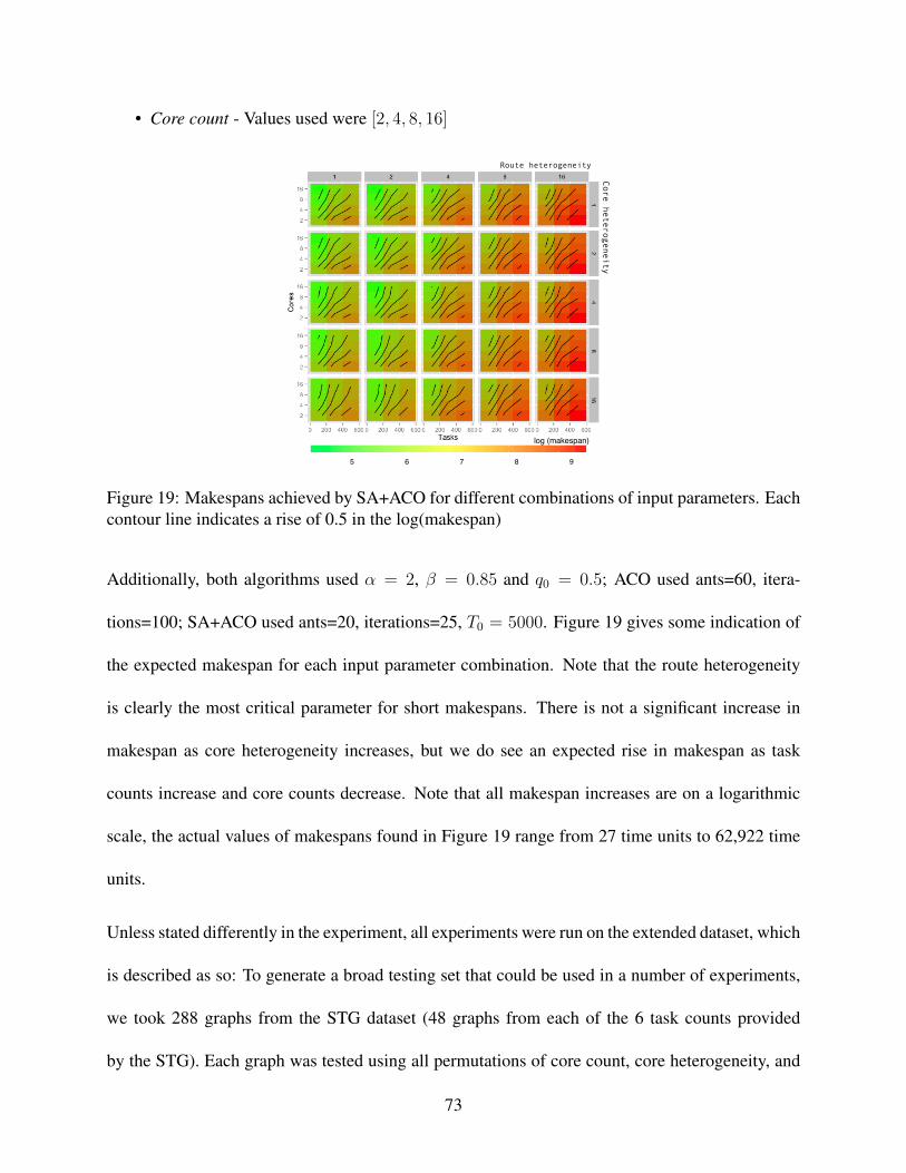
• Core count - Values used were [2, 4, 8, 16]

65 7 8 9

log (makespan)

Route heterogeneity

Core heterogeneity

Figure 19: Makespans achieved by SA+ACO for different combinations of input parameters. Eachcontour line indicates a rise of 0.5 in the log(makespan)

Additionally, both algorithms used α = 2, β = 0.85 and q0 = 0.5; ACO used ants=60, itera-

tions=100; SA+ACO used ants=20, iterations=25, T0 = 5000. Figure 19 gives some indication of

the expected makespan for each input parameter combination. Note that the route heterogeneity

is clearly the most critical parameter for short makespans. There is not a significant increase in

makespan as core heterogeneity increases, but we do see an expected rise in makespan as task

counts increase and core counts decrease. Note that all makespan increases are on a logarithmic

scale, the actual values of makespans found in Figure 19 range from 27 time units to 62,922 time

units.

Unless stated differently in the experiment, all experiments were run on the extended dataset, which

is described as so: To generate a broad testing set that could be used in a number of experiments,

we took 288 graphs from the STG dataset (48 graphs from each of the 6 task counts provided

by the STG). Each graph was tested using all permutations of core count, core heterogeneity, and

73

route heterogeneity with a routing default cost of 1.


Due to the nature of the problem under test, there is a large desire to test exhaustively and under-

stand precisely which conditions the provided algorithm is effective for. To enable this large-scale

testing, the experimental platform was a cluster of thirty-two computers and a master node. The

proposed algorithm was encapsulated as a stand-alone C++ executable, and the python jug [77]

framework was used to assist in running multiple iterations of the solution concurrently on the

clustered computers. All C++ was compiled with g++ 4.4.6 using the -O3 flag. To assist other

researchers, our exact experiment data, testbed code, and solution code will be made open source.

The master computer has an 8-core Intel Xeon X3470 2.94GHz processor and 8GB memory. It

is running CentOS 6.0, python 2.6, and jug 0.9.2. Each homogeneous clustered computer uses a

Dell D610 blade mesh with two Intel Xeon E5646 12-thread processors, for a total of 24 hardware

threads per computer. Each computer has 36GB of memory and is running CentOS 6.0, python

2.6, and jug 0.9.2. Jug was configured to use a filesystem (NFS) backend for locking and task

synchronization.

5.9.2 Comparing To Known Optimal

The base STG dataset (e.g. homogeneous cores and no communication delays) included known

optimal scores for all four core counts used. Comparing both the nonhybrid ACO and the hybrid

ACO+SA algorithms to known optimal values will give an understanding of how well these algo-

rithms fit into other work in the general area of MCDO. The primary point of this experiment is to

74

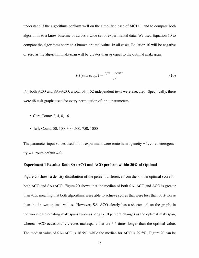
understand if the algorithms perform well on the simplified case of MCDO, and to compare both

algorithms to a know baseline of across a wide set of experimental data. We used Equation 10 to

compare the algorithms score to a known optimal value. In all cases, Equation 10 will be negative

or zero as the algorithm makespan will be greater than or equal to the optimal makespan.

PI(score, opt) =opt− score

opt(10)

For both ACO and SA+ACO, a total of 1152 independent tests were executed. Specifically, there

were 48 task graphs used for every permutation of input parameters:

• Core Count: 2, 4, 8, 16

• Task Count: 50, 100, 300, 500, 750, 1000

The parameter input values used in this experiment were route heterogeneity = 1, core heterogene-

ity = 1, route default = 0.

Experiment 1 Results: Both SA+ACO and ACO perform within 30% of Optimal

Figure 20 shows a density distribution of the percent difference from the known optimal score for

both ACO and SA+ACO. Figure 20 shows that the median of both SA+ACO and ACO is greater

than -0.5, meaning that both algorithms were able to achieve scores that were less than 50% worse

than the known optimal values. However, SA+ACO clearly has a shorter tail on the graph, in

the worse case creating makespans twice as long (-1.0 percent change) as the optimal makespan,

whereas ACO occasionally creates makespans that are 3.5 times longer than the optimal value.

The median value of SA+ACO is 16.5%, while the median for ACO is 29.5%. Figure 20 can be

75

0

1

2

0.0 −0.5 −1.0 −1.5 −2.0 −2.5 −3.0 −3.5Percent Change From Optimal Score

Den

sity

Algorithm

ACO

SA+ACO

Figure 20: Comparison to known optimal values made by using Equation 10. Thick vertical linesindicate data median. 1152 samples per Algorithm.

misleading in that a small change in absolute execution time can result in a large difference in

percent change. Table 2 helps to clarify the results of Figure 20 into absolute difference in time

units and shows that in all subsets considered SA+ACO outperforms ACO.

Cores Median OPT SA+ACO Median ACO Median2 1569.5 +22 +624 798 +91 +217.58 489 +158 +31316 343 +121.5 +317

Table 2: Comparison of Median Achieved Scores. Task sizes included are[50, 100, 300, 500, 750, 1000].

5.9.3 Runtimes of ACO and SA+ACO

While initial results from the experiment in Section 5.9.2 show that SA+ACO is outperforming

ACO on the version of the problem with the most assumptions, a critical question is how much

extra runtime is needed to achieve these better scores. An algorithm that exhibits exponential

runtime for linear increase in scores may rapidly become impractical.

76

Experiment Results: SA+ACO runs 60-90% faster than ACO.

0.00

0.02

0.04

0.06

0 100 200 300Time (in seconds)

Den

sity

Algorithm

ACO

SA+ACO

Figure 21: Density distribution of runtimes of SA+ACO and ACO.

Figure 21 shows that SA+ACO is consistently faster than ACO in terms of absolute runtimes.

SA+ACO finds solutions to all problems within 100 seconds(and typically in under 10 seconds),

whereas ACO finds requires up to 300 seconds to find solutions. Equation 11 was used to determine

that the minimum and maximum runtime differences were 60% and 90%.

PC(saaco, aco) =aco− saaco

aco(11)

5.9.4 Score Comparison of SA+ACO and ACO

This section compares the makespans found by SA+ACO and ACO across the entire input space.

There were 600 unique parameter combinations of core count, task count, route heterogeneity, and

core heterogeneity. For each parameter combination, we performed trials using 48 different graphs

77

1 2 4 8 16

24816

24816

24816

24816

24816

12

48

16

50 100 300 500 7501000 50 100 300 500 7501000 50 100 300 500 7501000 50 100 300 500 7501000 50 100 300 500 7501000Tasks

Cores

−20% −10% 0 10% 20%

Route heterogeneity

Core heterogeneity

Figure 22: Percent Change from ACO score to SA+ACO score across the entire range of inputparameters.

from the STG, resulting in a total of 28800 trials per algorithm. The percent difference between

SA+ACO scores relative to ACO scores is calculated using Equation 11.

Experiment Results: SA+ACO typically outperforms ACO

Figure 22 is a comparison of the performance of SA+ACO to ACO across a wide range of input

space. For utility in discussing, we adopt the following notation: cctcxrhch where cc = core count, tc =

task count, rh = route heterogeneity, and ch = core heterogeneity. Having a wildcard ∗ in any of

the locations references all versions of that parameter. Having two numbers separated by a colon

indicates an inclusive range. For any precise combination ijxkl the value shown in Figure 22 is the

median of 48 samples, where each sample is a different STG graph.

One of the most promising observations is the consistent improvement in makespans at 16300:1000x

1:2∗ .

78

This case of relatively low route heterogeneity and a large number of cores and tasks is exemplary

of current hardware trends in large scale computing. The effect is fairly independent with respect to

core heterogeneity, meaning that slight differences in core execution speeds should not disrupt the

improvement. Large computing grids with highly connected clusters are used to achieve speedups

on parallelized algorithms with huge numbers of tasks, with the goal being linear speedup in the

number of cores.

One of the least promising observations is at 8∗x

16∗ , where SA+ACO consistently performs worse

than ACO. Unfortunately, multiple attempts to dissect this failure have been unfruitful. One pos-

sibility is that the exact combination of 8 cores and 16 route heterogeneity is probabilistically

poor–there are enough routes (8*7) that multiple routes receive a high routing delay, but there are

not enough total routes to move onto cores that avoid these bottlenecks. When reaching 16 cores,

the number of routes increases drastically (from 42 to 16*15=240), and therefore poor routes can

be avoided. However, this possibility has not been qualitatively examined. As discussed in Section

5.10, the choice of route heterogeneity = 16 may be a poor input parameter choice that is changed

in future works.

A large performance increase is noticed at 4∗x

4∗, where SA+ACO is achieving makespans of 10-20%

better than ACO. The increase continues, but at a reduced rate of 0-10%, into 4∗x

8:16∗ , indicating that

for 4 cores and medium to high route heterogeneity SA+ACO is a good choice.

79


This section has introduced a new hybrid algorithm for solving the Multi-core Deployment Op-

timization (MCDO) problem. We have continued prior work on using ant colony optimization

(ACO) to solve MCDO problem, specifically by relaxing some of the assumptions of prior work

and by adding an initial simulated annealing (SA) step. The two metaheuristics are interleaved,

with the SA algorithm providing a seeding step for the pheromones matrix used inside the ACO

algorithm.

Comparison to known optimal solutions to the MCDO is possible for for a subset of the input

space due to the work by Tobita and Kasahara [70] in publishing the Standard Task Graph (STG)

Set, a dataset of concurrent application task execution time and precedence relations. Across 50

applications from the STG, and testing 2, 4, 8, 16 cores, the hybrid SA+ACO algorithm is shown

to acquire a median of 16.5% increase in makespan time versus the optimal solution. On the same

data, the nonhybrid ACO algorithm has a median increase in makespan of 29.5% over optimal.

However, optimal values are only available under a number of simplifying assumptions, such as

homogeneous cores and no routing delays. Relaxing these assumptions, we can only compare the

performance of SA+ACO to the nonhybrid ACO algorithm. With one exception, across all combi-

nations of the input parameters (core count, task count, core heterogeneity, routing heterogeneity)

SA+ACO is able to find makespans that are 0% to 30% better than those found by ACO alone.

Moreover, the runtime of the SA+ACO algorithm is typically 1/3 or less of the runtime of the ACO

algorithm. The SA+ACO algorithm is shown to generate solutions 25% worse than nonhybrid

ACO algorithm for a small class of input spaces where the routing heterogeneity is quite high (e.g.

80

up to 16x difference in the routing time of two cores) and the number of cores is 8. More work is

required to determine the exact cause for this isolated failure.

For future work, we would like to create a toolkit to generate of executable solutions, which can

then be profiled and compared with the resource usage predicted by the objective function. We

are also interested in exploring multi-objective approaches, such as minimizing the energy con-

sumption of the solution. In addition, there are a number of other algorithms for solving MCDO

problems that we would like to compare against.

From our research on Multi-core Deployment Optimization, we learned the following important

lessons:

1. Using Simulated Annealing To Seed Ant Colony Optimization is Quick and Effective.

The simulated annealing algorithm described in this paper cools into a greedy local search.

Constructing valid solutions in a local search is typically much quicker than running an iter-

ation of an ant colony solution, as the local search simply permutes valid solutions into other

valid solutions instead of creating valid solutions. However, the ant colony optimization

we define is more effective than random-search simulated annealing at reusing information

and performing guided exploitation of a solution space. The combination of these two meta-

heuristics is shown to be highly effective and worthy of continued research. A future research

may include seeding the ACO pheromone matrix with the best N solutions.

2. Routing Heterogeneity is Critical to Successful Shortest Paths. The results in this work

show that routing heterogeneity is critical to shorter makespans. However, the open-ended

assumption of arbitrary routing heterogeneity may be too general to be practical. Modern

81

computer systems are often connected in a 2d plane, where each core has a NSEW con-

nection to its neighbor. Using taxicab distance and assuming that each hop from neighbor

to neighbor introduces a fixed routing delay, the interaction of routing heterogeneity and

number of cores can be determined. For example, if all cores are known to contain all four

NSEW connections, then the maximal routing heterogeneity is simply the largest taxicab

distance. If cores are arranged in a square grid, this taxicab distance will typically equal

2 ∗ (√cores − 1), and the maximal routing heterogeneity can be fixed to this value. Future

work in this area should use different time units for routing and computation delays, and use

accurate hardware models of routing delay.

3. With Relaxed Assumptions, Heuristic Creation Becomes Harder During the execution

of an ant colony optimization, the heuristic function will typically be executed hundreds,

if not thousands, of times each time an ant creates a tour. This requires that the heuristic

function execute quickly, but this requirement for rapid execution can be difficult to achieve

in highly interconnected solution spaces. For example, considering faster processors to be

more desirable can leave out information about routing delays, ending in an overall adverse

effect on solution quality. Future work should explore statically calculated data structures

shared by all ants to help to enable rapid heuristic calculation, such as summary values for a

core’s routing centrality and a task’s need for routing centrality.

The SA+ACO code, the benchmarking code (using the python jug framework), and the extended

dataset containing all of our results are available at https://github.com/VT-Magnum-Research/SA-

ACO.

82

6 Large-Scale Distributed Smartphone Emulation


To address the need for realistic smartphone testing and experimentation environments, we intro-

duce Clasp, a system for dynamically interfacing with a distributed cloud of smartphone emulators.

Clasp provides a queue-based system for job submission, abstracts differences between mobile OS

versions, manages the orchestration, execution, and recovery needed when programmatically using

smartphone emulators, and provides both Hypertext Transfer Protocol (HTTP) Representational

state transfer (REST) and WebSocket Application Programming Interfaces (APIs) for enabling

real-time interaction and control of remote emulators.

This work provides the following contributions to creation of large-scale smartphone testbeds:

• An extensive survey of existing research in the area of large-scale smartphone testing, ex-

perimentation, and distributed emulation

• Detailed descriptions for a number of architectural challenges faced when building a dis-

tributed smartphone emulation system

• Quantitative data exposing the engineering challenges encountered with large-scale smart-

phone emulation

• Clasp, A system for large-scale Android emulation comprising thousands of devices and tens

of worker hosts, including:

– Real-time HTTP and WebSocket APIs for launching, controlling, and querying dis-

83

tributed emulators

– A remoting wrapper library enabling local Object-Oriented (OO)-based programming

of large number of remote emulators

– Quantitative analysis of Clasp’s performance

6.2 Challenges of Large-Scale Distributed Smartphone Emulation

There is a substantial demand for testbeds for large-scale smartphone systems in diverse areas such

as academic study, military applications, and commercial ventures. However, most smartphone

emulators are resource-intensive and error-prone. To support a range of mobile OS versions, a

distributed emulation system has to successfully couple multiple legacy codebases in the form of

older smartphone emulators and operating systems. In addition, the diverse range of mobile OS

versions and emulator software versions has resulted in a vast array of software flags, many of

which have complex relationships such as mutual exclusion or hard dependence. For example,

simulating a user button press requires a different approach upon the version of Android OS in use,

and the button press must be communicated in a different manner depending upon the version of

the Android emulator in use. In addition, there is often no clear manner to check for success or

failure of an attempted task, such as a simple button press.

This section outlines the major challenges faced when creating a large-scale distributed smartphone

emulation system such as Clasp.

84

6.2.1 Error-prone, Resource Intensive Agents Increase the Difficulty of Creating Stable

Large-Scale Simulations

Orchestrating thousands of mobile device emulators across hundreds of host computers requires

each node to be resilient to emulator failures. A node should be capable of detecting and recovering

from such failures without affecting the remaining testbed operations, including any ongoing task

currently running on the emulator. Detection of failures is challenging, as smartphone emulators

are virtual machines that can maintain external state even when the internal operating system has

become unresponsive. This is generally termed the Halting problem. Moreover, approaches to

recover from failure are also unclear, as there is no information available external to the emulator

VM as to why a failure occurred or what internal state may have been affected.

Section 6.3.2 describes how we address these management issues by creating an emulator heartbeat

signal and isolating units of work into small tasks that can more easily be checked for errors.

6.2.2 Multiple Software/Hardware Platforms Increase Difficulty of Simulation

The range of mobile devices that might be connected to the IoT is very large, and practitioners can

expect to see hundreds of different combinations of software and hardware on the mobile devices.

To successfully simulate this condition, a system must be able to orchestrate multiple versions of

mobile devices, as well as include physical mobile device hardware into the simulation results.

Each version of a mobile device OS can have widely different options, including different config-

uration option sets, different user input mechanisms, and different resource consumption charac-

teristics when emulated [78]. Creating a single interface that can span this range of technology is

85

difficult [59, 78].

While technologies such as the Android emulator allow emulation of a range of Android versions,

there are a large number of differences between each version. For example, pressing mobile device

buttons, such as the Home, Power, or Volume Up buttons, uses different mechanisms on different

versions of the Android emulator. Moreover, Android emulators running different Android OS

versions can consume wildly different resources, such as CPU and RAM, on the host system. For

example, a 2GHz 8GB x86 host can run four properly-configured Android 4.2 emulators, but the

same host machine would have substantial difficulties running four Android 2.3 emulators. Section

6.3.5 describes how we address this challenge using node resource feedback loops.

6.2.3 Large-scale IoT/mobile device Orchestration Requires a Complex Input Model

Each mobile device has a complex input model, spanning static inputs such as device configuration

and pre-loaded data, to time-series inputs such as sensor input during the course of the simulation,

and dynamic input such as user input on the device screen. Dynamic inputs can also be generated

from other systems during the simulation. A concise, repeatable method for specify this wide range

of inputs is needed.

Section 6.3 describes how Clasp enables multiples types of specific, repeatable input via external

modules, such as the Persona module that can create a range of realistic contacts.

86

6.3 Research Gap 3 Solution Details

Clasp is a system to enable large-scale emulation and control of Android emulators. Clasp also

enables realistic large-scale testing of existing services, such as web services enabling the Internet

of Things. Clasp is designed to be executed as a remote web service whereby end-user clients can

remotely trigger device launches, submit device tasks, and receive device output. Clasp exposes

two remote interfaces, a HTTP REST for simple client interaction, and a WebSocket interface for

more complex session-based bidirectional interaction. Clasp is a highly distributed system that

uses the Actor concurrency model to enable simpler reasoning about distributed system state.

6.3.1 Architecture of Clasp

In order to integrate with third-party Internet-based services, such as those running on the Internet

of Things, Clasp must bridge its distributed set of Actors, most of which are not publicly routable,

with these external agents. It is critical that these remote services can perform actions such as

launching new emulators, accessing device details, sending files such as applications to these de-

vices, etc. As shown in Tables 4 and 3, there is substantial ability for remote clients to introspect

Clasp. This section outlines the major design decisions that enable remote clients to easily interact

with the network of mobile devices provided by Clasp.

Figure 23 shows the main components that allow remote Internet-based services to communicate

with devices run inside Clasp in a bi-directional manner. Figure 23 also shows worker nodes that

are not available from the public Internet, which is common for security and cost reasons.

87

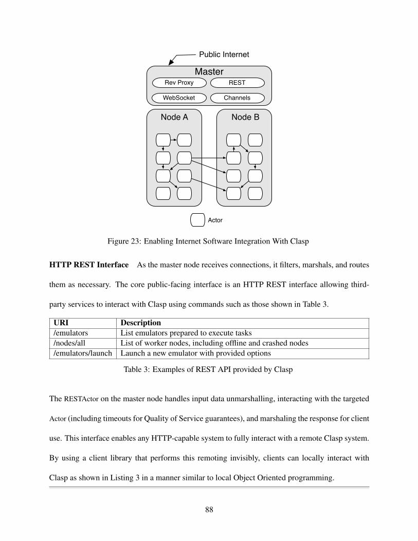
Node B

Actor

Node A

MasterREST

WebSocket

Rev Proxy

Channels

Public Internet

Figure 23: Enabling Internet Software Integration With Clasp

HTTP REST Interface As the master node receives connections, it filters, marshals, and routes

them as necessary. The core public-facing interface is an HTTP REST interface allowing third-

party services to interact with Clasp using commands such as those shown in Table 3.

URI Description/emulators List emulators prepared to execute tasks/nodes/all List of worker nodes, including offline and crashed nodes/emulators/launch Launch a new emulator with provided options

Table 3: Examples of REST API provided by Clasp

The RESTActor on the master node handles input data unmarshalling, interacting with the targeted

Actor (including timeouts for Quality of Service guarantees), and marshaling the response for client

use. This interface enables any HTTP-capable system to fully interact with a remote Clasp system.

By using a client library that performs this remoting invisibly, clients can locally interact with

Clasp as shown in Listing 3 in a manner similar to local Object Oriented programming.

88

import clasp._

object Test {

def main(args: Array[String]) {

val clasp = Clasp(host="masternode.clasp.com", port=80)

val emulators: Seq[Emulator] = clasp.list_emulators

if (emulators.length < 100) {

// Clients can modify this as needed

val options = new EmulatorOptions

clasp.launch_emulator(options)

}

// Logic using emulators goes here

}

}

Listing 3: Using library to transform HTTP REST API into Object Oriented programming

WebSocket Interface The primary limitation of the above approach is that Clasp cannot broad-

cast events, such as emulator task complete, back to client systems. In general, HTTP REST clients

must continually poll to determine if new server events have occurred. Most systems comprising

the Internet of Things must consider the resource cost, such as battery usage, of constantly access-

ing the network and processing response data. One method of addressing this resource utilization

89

is to utilize a bidirectional protocol in which Clasp can alert the remote system when events of in-

terest happen. Clasp uses the WebSocket protocol to enable bidirectional data transfer on a single

TCP port. The WebSocketActor on the master node detects incoming WebSocket requests and cre-

ates a worker Actor for each connection. To avoid the resource cost of maintaining multiple open

TCP connections and simplify Clasp’s architecture, each connection is multiplexed into a number

of publisher-subscriber channels by the ChannelActor. By subscribing to channels, such as those

shown in Table 4, clients can send direct messages to Actors, who either reply directly or broadcast

messages to all clients subscribed to the channel.

Channel Description/emulator/<ID>/logs Receive all logs from emulator <ID>/devices Updates about changes in any device’s state, such as Crashed, Booting,

Ready/node/<ID>/resources Receive updates on node <ID>’s resource usage, such as RAM and

CPU

Table 4: Examples of WebSocket publisher-subscriber channels available

An important consideration was enabling first-class support for the WebSocket interface so that

clients could interact with Clasp without ever using the HTTP interface. The main challenge is how

to mingle current state snapshots, such as those provided by the REST interface, with streaming

updates, such as those provided by the WebSocket interface. Adding separate WebSocket channels

for determining current status creates nontrivial client-side threading issues. For example, if a

client requests current status from one channel, and also requests status updates from another

channel, the order of responses becomes important. To remove this client-side complication, Clasp

replays all channel history to any new client connections. In this manner, new clients are always

provided the current state as a stream of updates, and after this updates are provided as they are

generated. This is accomplished by storing all channel messages to log files, and replaying the log

90

file when a new client connects. A future iteration of Clasp may include flattening these channel

log files occasionally to prevent sending large amounts of extra data to clients, but the current use

cases have not required this.

Hybrid Remote API Usage Clients may want to use both the WebSocket remote API, which

is excellent for streaming information such as real-time logs, and HTTP remote API, which is

excellent for one-time tasks such as sending emulator launch commands. To enable hybrid usage,

all WebSocket channel messages are fully-valid JSON objects, such as the one shown in Listing

4, and are marshaled identically to the HTTP REST API. The primary difference is that the REST

API will return an array of JSON objects in some scenarios while the WebSocket interface will

send each object as a separate message.

{

"ip": "10.0.0.2",

"status": "Booting",

"emulators": 0,

"uuid": "931a313a-a986-456b-9172-7b355b19db25",

"asOf": "2014-09-30T21:00:51Z"

}

Listing 4: JSON Format Shared by Clasp’s HTTP and WebSocket Interfaces

Connecting to TCP services on Worker Nodes Finally, we have found substantial value in

selectively allowing direct connections to various services, such as the Android Debug Bridge

91

(adb) and Virtual Network Computing (vnc), from devices on the public internet. These proto-

cols are challenging to adapt to an Actor-based programming model, and therefore we created the

RevTCPproxyActor, which opens and maintains a dedicated TCP proxy between a worker node and

the master node. Public internet clients may then connect to the opened port on the master node,

and their traffic will be invisible routed through our private network to the target service running

on the worker node. An example of this is discussed in more detail in Section 6.3.3.

6.3.2 Complex, Error-Prone Agents

As discussed in Section 6.2.1, mobile devices and mobile device emulators are complex agents in

our system, and are prone to errors, including errors that are nontrivial to detect such as becoming

unresponsive to user input. Clasp uses two different approaches to address the challenge of dealing

with these error-prone agents. First, each Android emulator is directly monitored by an Actor using

the state diagram shown in Figure 24. Second, the work delivered to each emulator is segmented

into Tasks, which are delivered in serial to an emulator and therefore allow failures to be isolated

to one Task. We discuss each approach in detail in this section.

Booting Booted

Not Booted

Timeout

Heartbeat Fail; Shutdown;Task Fail

Heartbeat Pass

Figure 24: EmulatorActor Finite State Machine

The state diagram above shows potential states for the EmulatorActor, which monitors a single

92

Android emulator process. The EmulatorActor detects any premature exit of the emulator process,

and will attempt to restart the process based on a recovery strategy, such as restart three times,

then escalate the failure. The EmulatorActor also periodically attempts direct interaction with the

underlying emulator, and terminates the emulator process if a response is not received in a timely

manner. The EmulatorActor can additionally monitor the time taken for Task execution and indicate

failure if a given tasks takes longer than the default timeout provided for that task (defaults to 5

minutes).

Other components within Clasp interact with the EmulatorActor, which in turn manages interac-

tion with the emulator process. In this manner, Clasp can isolate and recover from failures of the

underlying emulator process. To enable responsiveness while interacting directly with the emu-

lator process, the EmulatorActor uses Futures and Promises to handle worker thread creation and

response processing.

6.3.3 Providing User Input To Android Emulators Using Clasp

Control of mobile devices requires user input events, such as button presses and screen touch

events. Even simplistic applications can require complex patterns of user input to transition be-

tween application states. For example, sending a text message with the default SMS application

on the Android 4.0 platform requires at least five key events (enter application, tap New Message

button, tap To field, tap Message field, tap Send button). It is infeasible to manually provide this

user input to hundreds of devices, and therefore automation is critical. However, automation of

user input can be extremely error-prone, as slight differences in application version can cause large

differences in the sequence of inputs required to reach a target state. Moreover, external events

93

can cause view hierarchy updates, such as overlay windows for incoming messages, due to the

event-driven nature of the Android platform. Therefore it is important to allow automation from a

guaranteed static state, and to enable easy debugging of the user input process.

Manual User Input and Feedback is the most direct method of user control of the mobile device

emulator. The distributed nature of Clasp makes this challenging, as each emulator is running on a

remote host. Figure 25 shows an overview of Clasp’s approach for enabling manual user feedback

and control of emulators.

Virtual Framebuffer

QEMU

VNC

Process IO

Actor Worker Node

Live View+Control From Web Browser

HTML5 VNC Viewer

Dynamic WebSocket Log

Figure 25: Real-time view and control of remotely-hosted mobile device emulators

As discussed in Section 6.3.2, mobile device emulators are error prone processes that are wrapped

with an Actor that monitors the emulator process. For each emulator, the Actor also creates a virtual

framebuffer that the emulator will be rendered into. This framebuffer is precisely sized to preserve

memory on the worker node. A lightweight Virtual Network Computing (VNC) server is launched

on the worker node, to allow remote access and control of this framebuffer. This VNC server must

be configured with the proper keymaps for controlling the Android emulator, which is non-trivial

as different versions of Android OS use different keymaps, and customized Android versions often

extended these default keymaps with additions such as keys for Bluetooth control.

94

To enable view and control any emulator running inside of Clasp, the web interface embeds a

HTML5 VNC viewer that can be used by any modern web browser. A persistent WebSocket con-

nection is used to enable bi-directional VNC communication. Moreover, the output of the emulator

process is captured in real-time, and the WebSocket protocol is used to deliver this information to

the web browser in real time. The HTTP+WebSocket API defined in Section 6.3 is used by the

web interface to communicate with the Clasp system, enabling actions such as 1) listing connec-

tion information for running mobile device emulators, 2) registering for update messages, such as

log information, for a specific emulator, and 3) sending control actions to emulators.

While not shown in Figure 25, a non-trivial challenge is that most worker nodes do not have

publicly-routable IP addresses. Therefore direct connections between the client computer running

Clasp’s web interface and the host running Clasp’s worker nodes are not possible. To address

this, the Clasp master node acts as a proxy for each worker node. For protocols such as HTTP

multiple proxy libraries are available, but for more recent or complex protocols such as VNC and

WebSockets this is a non-trivial task. The master node dynamically establishes these proxies as

needed to avoid wasting resources if a worker node is not being actively accessed.

Automated User Input is easily achieved with the Android Monkey tool, which allows generation

of a stream of user input events, such as swipes or button taps.

6.3.4 Addressing Failure and Recovery of Smartphone Emulators

For each mobile OS version, Clasp contains an appropriate heartbeat signal that is used to deter-

mine if the mobile OS running inside the emulator is responding appropriately. For some Android

versions, such as Android 4.0, there is an equivalent ping command available. For older OS ver-

95

sions, this is simulated using commands that have no side effects and have been quantitatively

proven to respond quickly, such as the list sensors command. By sending this heartbeat signal to

running emulators on a regular basis Clasp can easily determine if emulators are still responsive

within acceptable quality of service limits.

To address job failure detection and recovery, Clasp defines a number of small operations, such as

install package. For these small tasks a combination of output checks, such as looking for specific

response strings e.g. Success, timeouts e.g. 30 seconds, and followup commands e.g. List Installed

Packages is used to determine if a task has succeeded or failed. By chaining series of these reliable

tasks together a full sequence of behavior can be executed with confidence that each item was

completed successfully.

6.3.5 Enabling Emulation of Multiple Software/Hardware Platforms

As discussed in Challenge 6.2.2, each version of a mobile device OS can have widely different op-

tions, including different configuration option sets, different user input mechanisms, and different

resource consumption characteristics when emulated.

To enable uniform interaction with Android emulators, regardless of version, we use the Abstract

Factory design pattern to generate concrete classes specific to interaction with that version of An-

droid. This allows uniform interaction, including items such as hard button presses, screen taps,

and specification of configuration.

To deal with the challenge of vastly different resource consumption characteristics, each NodeActor

in the system monitors its own resource characteristics and shares that information with the NodeManager.

96

When a new emulator is requested, the NodeManager actively selects a worker node for the new em-

ulator based on the available resources of each worker node and the past resource consumption of

similar emulators.

6.3.6 Simplifying Simulation Input Model Using Modules

To address the need for the hundreds of different inputs needed when executing a large-scale ex-

periment, Clasp includes a number of configurable modules to automatically provide these inputs.

For example, Listing 5 initiates the Persona module, which will create realistic contact details

for the current mobile device user including photos, contacts, accounts, etc. By segregating the

input model in this manner, Clasp enables high customization while avoiding complexity unless

customization is needed. Each module can individually determine what data sources (e.g. file,

network stream, other emulator outputs, internal simulation) are used to generate inputs, as well as

ensure repeatability.

import clasp._

object Test {

def main(args: Array[String]) {

val clasp = Clasp(host="masternode.clasp.com", port=80)

val emulators: Seq[Emulator] = clasp.list_emulators

if (emulators.length < 100) {

// Clients can modify this as needed

val options = new EmulatorOptions

97

clasp.launch_emulator(options)

}

Persona.configureAll(emulators)

}

}

Listing 5: Using the Persona module to automatically configure emulator

6.4 Experimental Results And Validation

This section outlines multiple tests on individual components of Clasp, as well as experimental

analysis of the combined Clasp system. It also includes a case study of using Clasp to experimen-

tally benchmark web service performance.


We analyzed Clasp on the Android Tactical Application Assessment & Knowledge (ATAACK)

Cloud [59], which is a hardware platform designed to provide a testbed for cloud–based analysis

of mobile applications. The ATAACK cloud currently uses a 34 node cluster, with each cluster

machine containing Dell PowerEdge M610 blade running CentOS 6.3. Each node has 2 Intel

Xeon 5645® processors with 6 cores (supporting 12 independent hardware threads), as well as

36GB of DDR3 ECC memory shared between the 2 processors.

98

6.4.2 Analysis of Emulator Launch Times and Host Resource Consumption

This experiment shows Clasp’s resource consumption when launching large number of emulators

in multiple configurations, and provides a performance baseline for multiple scenarios. This exper-

iment showcases the various challenges of dealing with resource-intensive heterogeneous emula-

tors by exploring multiple scenarios, such as overloading worker nodes and launching emulators in

step versus in tandem, and establishing expected coarse host resource consumption characteristics

for these scenarios. This experiment provides a critical baseline for future research in the area of

Distributed Emulation, as it quantitatively outlines numerous challenges faced.

Node Resources Consumed Per Emulator Figure 26 shows the host resource consumption

pattern created by an emulator launch. To create Figure 26, three emulators were launched in serial

with an eight minute gap between each launch to avoid interactions. Each emulator remains online

once launched so that Figure 26 can show any potential additive effects resulting from launching

emulators while other emulators are executing.

Each worker node used in this scenario has 36GB of RAM and two hyper-threaded 6 core 2.4GHz

processors, exposing a total of 2processors/1 ∗ 6cores/processor ∗ 2threads/core = 24threads/1. Therefore,

a 2% decrease in real memory roughly equals ≈720MB of consumed RAM, and 1% decrease of

the ≈2400% total CPU available equals ≈600MHz.

Each emulator consumes a non-trivial portion of real memory, around 720MB, as shown by the

blue boxes in Figure 26. Multiple important CPU consumption patterns are also exposed in Figure

26, such as boot spiking, steady-state consumption, heartbeat spiking, and interference effects.

99

94

96

98

100

% F

ree

RAM

0

1

2

3

4

5

6

0 2 4 6 8 10 12 14 16 18 20Minutes

% T

otal

CP

UCPU Metric

System

User

Wait

CPU

Figure 26: Node Resources Consumed on Emulator Boot with No Hardware Acceleration

Boot spiking is our terminology for the clear increase in CPU consumption as each emulator’s

VM is loaded into RAM and booted, at times t0, t8, and t16. After the boot spikes complete, at

times t4,t12, and t20, the steady-state consumption effect is the CPU cost of maintaining the idle

emulator. When Clasp sends a heartbeat to each emulator, as indicated by the triangle-tipped line

segments, there is a noticeable heartbeat spike effect. The heartbeat spike is our first example of

interference effects, where the effect is more pronounced with larger number of emulators. This

is only slightly apparent in Figure 26 by noticing the heartbeat spikes become more severe from

t4−8 to t12−16, and will be explored more in the next section. Later results show that interference

effects are apparent in multiple scenarios, such as communicating with emulators through adb and

the severity of boot spiking, as formalized in Equation 12. These interference effects, plus higher

levels of wait time, lead us to conclude that Android emulators share some core components. For

example, communication with a single Android emulator is often multiplexed through a server

100

running inside the Android Debug Bridge (adb), leading to a bottleneck when attempting to com-

municate with multiple emulators. Future work in large-scale distributed mobile device emulation

should make a determined effort to reduce these shared components as much as possible.

CPUboot = CPU0 +N ∗ Emulators (12)

Worker Node Degradation When Overloaded Figure 27 shows the resource consumption pat-

tern resulting from overloading a worker node by launching one non-hardware-accelerated Android

4.0 emulator every eight minutes until 80 emulator launches had been attempted. Emulator boot

spikes are clearly visible at regular intervals from time t0 to t11 as emulator launches were being

triggered, while time t11 to t13 shows the steady-state behavior as seen by the stabilization of the

RAM, CPU, and Swap metrics.

An initial experiment with 20 emulators was used to predict the failure point of the worker nodes,

by linearly projecting the measured RAM and CPU consumption. Upon stressing the worker

nodes to this failure point, we were only able to sustain 65 emulators at acceptable conditions,

due to large delays introduced by page swapping when worker node memory dropped below 30%.

As shown by Figure 27, the experiment used at most 60% of our available CPU capacity, while

the available RAM decreases linearly. Once available RAM drops below 30% (as configured by

the kernel swappiness setting), Linux Swap file Page Outs begin to increase. Clasp continually

sends heartbeats to emulators to ensure they are operating within acceptable limits. Therefore,

as the Swap file is used more aggressively Clasp begins to automatically shut off emulators that

are unresponsive and not currently running any tasks. For time t8−12 Figure 27 shows emulator

101

launches continuing to be triggered, and Clasp consistently terminating emulators that are deemed

to be unresponsive. This RAM bottleneck causes a launch cycle in Clasp where emulators being

launched are actively in RAM and are therefore responsive to heartbeats, while emulators already

launched are paged out and are therefore terminated.

Future work in this area will explore configuring emulators to use less memory, such that the

available CPU is fully utilized, and more intelligent reaction of heartbeat failures due to RAM

bottlenecks.

Figure 27: Worker Node Degradation WhenLaunching 80 Emulators with Clasp

y = 175 + 1.3 ⋅ x, r2 = 0.963

y = 46 + 0.18 ⋅ x, r2 = 0.807

50

100

150

200

250

0 20 40 60Active Emulators

Boo

t Tim

e (s

econ

ds)

Acceleration

None

VT−x

Figure 28: Android 4.0 x86 Emulator Boot TimeAs a Function of Emulators Already Running(bars indicate SEM)

Emulator Launch Times As discussed above, Android emulators share core components, such

as access to the underlying hardware virtualization, and access to running Android emulators is

102

typically multiplexed though a single Android Debug Bridge (adb) instance. For these reasons, it

is common to see emulator launch times increase with the number of emulators already executing

on that machine, as shown in Figure 28. Clasp correctly anticipates emulator boot time lengthening

on fully-loaded worker nodes and ensures the boot timeout window is large enough to address this

dynamic behavior.

Figure 28 is limited to 60 emulators to avoid the effects caused by exhausting host resources such

as RAM and CPU.

While Figure 28 provides a clear overview of emulator boot performance as a function of running

emulators. As emulators share some resources, there is the potential that two emulators booting

concurrently increases resource contention to the level that serial booting is more effective. As

shown in Figure 28 this was not the case – there was no benefit to intentionally delaying emulator

launches.

6.4.3 Emulator Speed

A large concern with distributed emulation, especially on a platform such as Amazon EC2 that is

already virtualized, is the emulator performance. The Android emulator supports KVM virtualiza-

tion, which drastically increases performance, and some Amazon EC2 machines launch with the

vmx, indicating that they support nested virtualization and allow the Android emulator to access the

host virtualization support. This experiment shows the average performance difference achieved

on such platforms.

Figure 29 shows the result of executing six common emulator tasks: installing an application,

103

pressing a key, listing installed packages, listing available sensors, and uninstalling an application.

The most apparent effect is the drastic time difference between listing available sensors (less that

1 second) and all other shown tasks. Listing available sensors is done through a direct telnet

connection to Android OS running inside the emulator, while all other tasks shown are routed

through the Android Debug Bridge (adb). By occasionally experiencing delays as large as 20

seconds for a single key press, the adb binary can delay execution of an entire stream of tasks. It is

unclear at this time what causes these occasional large delays.

0

1

2

3

4

5

6

install keypress packagelist sensorlist uninstallTask

Dur

atio

n (s

econ

ds)

Acceleration

None

VT−x

Figure 29: Timing Common Tasks on Android 4.0 x86 Emulators. Two outliers are not shown:(None,install,15.5 seconds) and (None,keypress,13.5 seconds).

As shown by Figure 29, lack of hardware acceleration causes slowdowns of nearly 400% for some

common emulator tasks. Additionally, emulators with no hardware acceleration are suscepti-

ble to occasional long delays, as evidenced by the major outliers at (None,install,15.5 seconds),

(None,keypress,13.5 seconds), and (None,keypress,5.4 seconds).

104

6.4.4 Task Throughput of Clasp

To examine the performance of Clasp when executing large numbers of tasks, we measured the

time to complete various sized queues of emulator tasks. Total time for each task included sub-

mitting the task to Clasp, Clasp selecting an available emulator, delivering the task to the remote

worker node, task execution time, and delivery of the task result. To minimize noise and ensure

the measured item was Clasp instead of the specific emulator being executed, each task performed

zero interaction with the emulator and just returned a result containing the time it was executed.

No dependencies existed between tasks.

0

5

10

0 2500 5000 7500 10000Task Queue Length

Dur

atio

n (s

econ

ds)

11

8

5

2

ConcurrentEmulators

Figure 30: Task Queue Throughput Grouped By Active Emulators

As shown in Figure 30, the speed of task execution is linearly dependent upon the number of tasks

that are queued. However, as more emulators are available to execute tasks, the total processing

time decreases drastically.

105


This chapter introduces Clasp, a system for large-scale distributed smartphone emulation. Clasp

represents a substantial research and engineering effort that will have implications for areas such

as academia, government, military, and industry. From this research, we provide the following

contributions to the study of large-scale distributed emulation:

1. Clasp: A System for Dynamically Launching and Controlling a Distributed Cloud of

Smartphone Emulators. As discussed in Section 3.3, there are a small number of systems

with functionality approaching Clasp, and therefore we expect Clasp to become a valuable

research tool in areas such as mobile malware analysis [79].

2. A Literature Survey of Existing Research on Large-Scale Smartphone Testing. Section

3.3 provides an extensive survey of existing research in the area of large-scale smartphone

testing, experimentation, and distributed emulation.

3. Empirical and Architectural Guidance on Creating Large-Scale Smartphone Testbeds.

Section 6.4 quantitatively explains a number of the engineering challenges encountered

while building Clasp. Section 6.3 explains a number of design challenges that were ad-

dressed to ensure Clasp was easily compatible with the numerous other tools researchers

may wish to use while researching large-scale smartphone systems.

106

7 Conclusions & Lessons Learned

This dissertation presents new methods to address a number of key challenges within the field of

mobile cloud computing. After extensive review of mobile cloud computing research literature, the

core research gaps identified are 1) a loss of locational privacy in existing mobile cloud computing

systems 2) a shortage of mobile cloud computing specific algorithms enabling efficient use of cloud

Infrastructure as a Service, and 3) no available testing suites for conducting mobile cloud comput-

ing research. For each of these gaps in research gaps, this dissertation proposes a novel solution

based upon existing literature, implements the proposed solution, and experimentally validates the

result.

7.0.1 Summary of Contributions

Provide k-anonymity locational privacy through controlled reductions in locational preci-

sion. Presented in Chapter 4, Anonoly is an algorithm that can enforce user anonymity while

maintaining the convenience of location based services. Using real-world data gathered from user

mobile devices on the Dartmouth campus, Anonoly outperformed existing approaches by main-

taining anonymity for 6 out of 8 weeks tested. Results show Anonoly is able to successfully

preserve user anonymity even during extreme situations, such as a school holiday causing a 90%

drop in the number of active mobile cloud computing users.

Enable more effective execution of mobile cloud computing systems onto IaaS by creating a

method to precisely predict application performance at various resource usage levels, as well as a

method for rapidly deploying large mobile cloud computing applications onto cloud infrastructure.

107

Results from Chapter 5 show performance prediction is accurate to within 3% of performance

achieved even under worst-case conditions, and application quality of service is improved up to

30% using the SA+ACO deployment algorithm.

Create a flexible testbed for large-scale mobile cloud computing experimentation. Clasp,

presented in Chapter 6, is a distributed emulation system that can execute and manages thousands

of Android emulators running on tens of physical hosts. Clasp monitors all host resources and

emulator responsiveness and adapts to reductions in performance, enabling a consistent experience

across a range of. Clasp also exposes multiple interfaces using standard web technologies and

internally handles core differences between mobile OS versions, such as key mappings, to enable

simple interconnection with a range of existing research software.

108

8 Bibliography

[1] C. Ziegler, “Sensorly aims to keep coverage maps honest,” Downloaded from

http://www.engadget.com/2010/02/05/sensorly-aims-to-keep-coverage-maps-honest/,

Feb. 2010.

[2] OpenSignal, “Android fragmentation visualized,” July 2013. [Online]. Available:

http://opensignal.com/reports/fragmentation-2013/

[3] T. Ristenpart, E. Tromer, H. Shacham, and S. Savage, “Hey, you, get off of my cloud: ex-

ploring information leakage in third-party compute clouds,” in Proceedings of the 16th ACM

conference on Computer and communications security. ACM, 2009, pp. 199–212.

[4] T. Saponas, J. Lester, J. Froehlich, J. Fogarty, and J. Landay, “iLearn on the iPhone: Real-

Time Human Activity Classification on Commodity Mobile Phones,” University of Washing-

ton CSE Tech Report UW-CSE-08-04-02, 2008.

[5] J. Froehlich, T. Dillahunt, P. Klasnja, J. Mankoff, S. Consolvo, B. Harrison, and J. Lan-

day, “UbiGreen: investigating a mobile tool for tracking and supporting green transportation

109

habits,” in Proceedings of the 27th international conference on Human factors in computing

systems. ACM, 2009, pp. 1043–1052.

[6] C. Thompson, J. White, B. Dougherty, and D. Schmidt, “Optimizing Mobile Application

Performance with Model-Driven Engineering,” in Proceedings of the 7th IFIP Workshop on

Software Technologies for Future Embedded and Ubiquitous Systems, 2009.

[7] G. Rose, “Mobile phones as traffic probes: practices, prospects and issues,” Transport Re-

views, vol. 26, no. 3, pp. 275–291, 2006.

[8] P. Leijdekkers and V. Gay, “Personal heart monitoring and rehabilitation system using smart

phones,” in Proceedings of the International Conference on Mobile Business. Citeseer,

2006, p. 29.

[9] T. Das, P. Mohan, V. N. Padmanabhan, R. Ramjee, and A. Sharma, “Prism: platform for

remote sensing using smartphones,” in Proceedings of the 8th international conference on

Mobile systems, applications, and services, ser. MobiSys ’10. New York, NY, USA: ACM,

2010, pp. 63–76. [Online]. Available: http://doi.acm.org/10.1145/1814433.1814442

[10] C. Cornelius, A. Kapadia, and D. Kotz, “AnonySense: Privacy-aware people-centric sensing,”

Proceeding of the 6th Int’l Conf. on Mobile Systems, Applications and Services, 2008.

[11] A. Kapadia, N. Triandopoulos, and C. Cornelius, “AnonySense: Opportunistic and privacy-

preserving context collection,” Sixth International Conference on Pervasive Computing,

2008.

110

[12] H. Lu, N. Lane, S. Eisenman, and A. Campbell, “Bubble-sensing: A new paradigm for bind-

ing a sensing task to the physical world using mobile phones,” in Workshop on Mobile Devices

and Urban Sensing, IPSN. Citeseer, 2008.

[13] L. Sweeney et al., “k-anonymity: A model for protecting privacy,” International Journal of

Uncertainty Fuzziness and Knowledge Based Systems, vol. 10, no. 5, pp. 557–570, 2002.

[14] J. Schad, J. Dittrich, and J.-A. Quiané-Ruiz, “Runtime measurements in the cloud: observing,

analyzing, and reducing variance,” Proceedings of the VLDB Endowment, vol. 3, no. 1-2, pp.

460–471, 2010.

[15] M. R. Gary and D. Johnson, “Computers and Intractability: A Guide to the Theory of NP-

completeness,” 1979.

[16] H. Kasahara and S. Narita, “Practical multiprocessor scheduling algorithms for efficient par-

allel processing,” IEEE Transactions on Computers, vol. 33, no. 11, pp. 1023–1029, 1984.

[17] Y. Kwok and I. Ahmad, “Static scheduling algorithms for allocating directed task graphs to

multiprocessors,” ACM Computing Surveys (CSUR), vol. 31, no. 4, pp. 406–471, 1999.

[18] S.-T. Lo, R.-M. Chen, Y.-M. Huang, and C.-L. Wu, “Multiprocessor system scheduling with

precedence and resource constraints using an enhanced ant colony system,” Expert Systems

with Applications, vol. 34, no. 3, pp. 2071–2081, Apr. 2008.

[19] H. R. Boveiri, “ACO-MTS: A new approach for multiprocessor task scheduling based on ant

colony optimization,” pp. 1–5, 2010.

[20] “Google Play,” URL https://play.google.com/, 2013.

111

[21] K. Langendoen, A. Baggio, and O. Visser, “Murphy loves potatoes: Experiences from a pilot

sensor network deployment in precision agriculture,” in Parallel and Distributed Processing

Symposium, 2006. IPDPS 2006. 20th International. IEEE, 2006, pp. 8–pp.

[22] R. Baldawa, M. Benedict, M. F. Bulut, G. Challen, M. Demirbas, J. Inamdar, T. Ki, S. Ko,

T. Kosar, L. Mandvekar, A. Sathyaraja, C. Qiao, and S. Zawicki, “PhoneLab: A Large-Scale

Participatory Smartphone Testbed,” in NSDI 9th USENIX Symposium on Networked Systems

Design and Implementation. NSDI ’12, 2012.

[23] N. Brouwers and K. Langendoen, “Pogo, a middleware for mobile phone sensing,” in Pro-

ceedings of the 13th International Middleware Conference. Springer-Verlag New York, Inc.,

2012, pp. 21–40.

[24] A. Konstantinidis, C. Costa, G. Larkou, and D. Zeinalipour-Yazti, “Demo: a programming

cloud of smartphones,” in Proceedings of the 10th international conference on Mobile sys-

tems, applications, and services. ACM, 2012, pp. 465–466.

[25] M. Mokbel and C. Chow, “Challenges in preserving location privacy in peer-to-peer environ-

ments,” 2006.

[26] P. Kalnis, G. Ghinita, K. Mouratidis, and D. Papadias, “Preserving anonymity in location

based services,” 2006.

[27] B. Hoh and M. Gruteser, “Protecting location privacy through path confusion,” 2005.

[28] B. Gedik and L. Liu, “Location privacy in mobile systems: A personalized anonymization

model,” 2005.

112

[29] M. Gruteser and D. Grunwald, “Anonymous usage of location-based services through spatial

and temporal cloaking,” in Proceedings of the 1st international conference on Mobile systems,

applications and services. ACM, 2003, pp. 31–42.

[30] G. Iachello, I. Smith, S. Consolvo, M. Chen, and G. Abowd, “Developing privacy guidelines

for social location disclosure applications and services,” in Proceedings of the 2005 sympo-

sium on Usable privacy and security. ACM, 2005, pp. 65–76.

[31] M. Duckham and L. Kulik, “A formal model of obfuscation and negotiation for location

privacy,” Pervasive Computing, pp. 152–170, 2005.

[32] V. Ciriani, S. De Capitani di Vimercati, S. Foresti, and P. Samarati, “k-anonymity,” 2007.

[33] E. Shechtman, C. Yaron, and M. Irani, “Space-time super-resolution,” vol. 27, no. 4, pp.

531–545.

[34] L. Sweeney, “K-anonymity: A model for protecting privacy,” in International Journal on

Uncertainty, Fuzziness and Knowledge-based Systems, vol. 10, no. 5, 2002, pp. 557–570.

[35] K. Emam and F. K. Dankar, “Protecting privacy using k-anonymity,” vol. 15, no. 5, 2008.

[36] J. Kong, “Formal notions of anonymity for peer-to-peer networks.”

[37] J. Bao, H. Chen, and W. Ku, “Pros: a peer-to-peer system for location privacy protection on

road networks.” in GIS’09, 2009, pp. 552–553.

[38] C. Bettini, X. S. Wang, and S. Jajodia, “Protecting privacy against location-based personal

identification,” in In Proc. of the 2nd VLDB Workshop on Secure Data Management (SDM

’05), vol. LNCS 3674. Springer Berlin / Heidelberg, 2005, pp. 185–199.

113

[39] G. Ghinita, P. Kalnis, and S. Skiadopoulos, “Privé: anonymous location-based queries in

distributed mobile systems,” in Proceedings of the 16th international conference on World

Wide Web, ser. WWW ’07. New York, NY, USA: ACM, 2007, pp. 371–380. [Online].

Available: http://doi.acm.org/10.1145/1242572.1242623

[40] M. F. Mokbel, C.-Y. Chow, and W. G. Aref, “The new casper: query processing for

location services without compromising privacy,” in Proceedings of the 32nd international

conference on Very large data bases, ser. VLDB ’06. VLDB Endowment, 2006, pp.

763–774. [Online]. Available: http://dl.acm.org/citation.cfm?id=1182635.1164193

[41] S. Mascetti, C. Bettini, X. Wang, D. Freni, and S. Jajodia, “Providenthider: An algorithm to

preserve historical k-anonymity in lbs,” in Mobile Data Management: Systems, Services and

Middleware, 2009. MDM ’09. Tenth International Conference on, may 2009, pp. 172–181.

[42] H. Chen, A. M. K. Cheng, and Y.-W. Kuo, “Assigning real-time tasks to heterogeneous pro-

cessors by applying ant colony optimization,” Journal of Parallel and Distributed Computing,

vol. 71, no. 1, pp. 132–142, Jan. 2011.

[43] T. D. Braun, H. J. Siegel, N. Beck, L. L. Bölöni, M. Maheswaran, A. I. Reuther, J. P. Robert-

son, M. D. Theys, B. Yao, and D. Hensgen, “A comparison of eleven static heuristics for

mapping a class of independent tasks onto heterogeneous distributed computing systems,”

Journal of Parallel and Distributed Computing, vol. 61, no. 6, pp. 810–837, 2001.

[44] E. Hou, N. Ansari, and H. Ren, “A genetic algorithm for multiprocessor scheduling,” Parallel

and Distributed Systems, IEEE Transactions on, vol. 5, no. 2, pp. 113–120, 1994.

114

[45] J. Brodkin. (2012, Oct.) Megadroid: 300,000 androids clus-

tered together to study network havoc. [Online]. Avail-

able: http://arstechnica.com/information-technology/2012/10/megadroid-300000-androids-

clustered-together-to-study-network-havoc/

[46] M. Bierma, E. Gustafson, J. Erickson, D. Fritz, and Y. R. Choe, “Andlantis: Large-scale

android dynamic analysis,” Note: Website http://minimega.org/ was not online as of Oct

2014.

[47] S. N. Hetu, V. S. Hamishagi, and L.-S. Peh, “Similitude: Interfacing a traffic simulator and

network simulator with emulated android clients.”

[48] (2014, Oct.) Manymo. [Online]. Available: https://www.manymo.com

[49] (2014, Oct.) Digitalocean. [Online]. Available: https://www.digitalocean.com

[50] D. S. Anderson, M. Hibler, L. Stoller, T. Stack, and J. Lepreau, “Automatic online validation

of network configuration in the emulab network testbed,” in Autonomic Computing, 2006.

ICAC’06. IEEE International Conference on. IEEE, 2006, pp. 134–142.

[51] B. Chun, D. Culler, T. Roscoe, A. Bavier, L. Peterson, M. Wawrzoniak, and M. Bowman,

“Planetlab: an overlay testbed for broad-coverage services,” ACM SIGCOMM Computer

Communication Review, vol. 33, no. 3, pp. 3–12, 2003.

[52] N. Van Vorst, M. Erazo, and J. Liu, “Primogeni: Integrating real-time network simulation

and emulation in geni,” in Principles of Advanced and Distributed Simulation (PADS), 2011

IEEE Workshop on. IEEE, 2011, pp. 1–9.

115

[53] S. McCanne, S. Floyd, K. Fall, K. Varadhan et al., “Network simulator ns-2,” 1997.

[54] X. Chang, “Network simulations with opnet,” in Proceedings of the 31st conference on Winter

simulation: Simulation—a bridge to the future-Volume 1. ACM, 1999, pp. 307–314.

[55] H. Soroush, N. Banerjee, A. Balasubramanian, M. D. Corner, B. N. Levine, and B. Lynn,

“Dome: A diverse outdoor mobile testbed,” in Proceedings of the 1st ACM International

Workshop on Hot Topics of Planet-Scale Mobility Measurements. ACM, 2009, p. 2.

[56] G. Werner-Allen, P. Swieskowski, and M. Welsh, “Motelab: A wireless sensor network

testbed,” in Proceedings of the 4th international symposium on Information processing in

sensor networks. IEEE Press, 2005, p. 68.

[57] D. Kotz, T. Henderson, I. Abyzov, and J. Yeo, “CRAWDAD trace

set dartmouth/campus/movement (v. 2005-03-08),” Downloaded from

http://crawdad.cs.dartmouth.edu/dartmouth/campus/movement, Mar. 2005.

[58] P. Turner, B. B. Rao, and N. Rao, “Cpu bandwidth control for cfs,” in Linux Symposium,

vol. 10. Citeseer, 2010, pp. 245–254.

[59] H. Turner, J. White, J. Reed, J. Galindo, A. Porter, M. Marathe, A. Vullikanti, and A. Gokhale,

“Building a cloud-based mobile application testbed,” Software Testing in the Cloud: Perspec-

tives on an Emerging Discipline, Nov 2012.

[60] Techempower’s frameworkbenchmarks. https://github.com/TechEmpower/FrameworkBenchmarks.

Accessed: 2014-09-01.

116

[61] W. Felter, A. Ferreira, R. Rajamony, and J. Rubio, “An updated performance comparison of

virtual machines and linux containers,” technology, vol. 28, p. 32.

[62] J. K. Lenstra and A. H. G. R. Kan, “Complexity of scheduling under precedence constraints,”

Operations Research, vol. 26, no. 1, pp. 22–35, 1978.

[63] P. Chretienne, E. G. Coffman, J. K. Lenstra, Z. Liu, and P. Brucker, Scheduling theory and its

applications. John Wiley & Sons, 1995, vol. 149.

[64] N. G. Hall and M. E. Posner, “Generating experimental data for computational testing with

machine scheduling applications,” Operations Research, vol. 49, no. 6, pp. 854–865, 2001.

[65] G. U. Srikanth, V. U. Maheswari, and A. P. Shanthi, “Tasks Scheduling Using Ant Colony

Optimization,” Journal of Computer . . . , Jul. 2012.

[66] H. Jin, H. Wang, H. Wang, and G. Dai, “An ACO-Based approach for task assignment and

scheduling of multiprocessor control systems,” Theory and Applications of Models of Com-

putation, pp. 138–147, 2006.

[67] H. Chen and A. M. K. Cheng, “Applying Ant Colony Optimization to the Partitioned Schedul-

ing Problem for Heterogeneous Multiprocessors,” pp. 1–4, Nov. 2012.

[68] D. Cordeiro, G. Mounié, S. Perarnau, D. Trystram, J. M. Vincent, and F. Wagner, “Random

graph generation for scheduling simulations,” p. 60, 2010.

[69] R. P. Dick, D. L. Rhodes, and W. Wolf, “TGFF: task graphs for free,” in CODES/CASHE

’98: Proceedings of the 6th international workshop on Hardware/software codesign. IEEE

Computer Society, Mar. 1998.

117

[70] T. Tobita and H. Kasahara, “A standard task graph set for fair evaluation of multiprocessor

scheduling algorithms,” Journal of Scheduling, vol. 5, no. 5, pp. 379–394, 2002.

[71] V. Cerny, “Thermodynamical approach to the traveling salesman problem: An efficient simu-

lation algorithm,” Journal of optimization theory and applications, vol. 45, no. 1, pp. 41–51,

1985.

[72] S. Kirkpatrick, C. D. Gelatt, and M. P. Vecchi, “Optimization by simulated an-

nealing,” Science, vol. 220, no. 4598, pp. 671–680, 1983. [Online]. Available:

http://www.sciencemag.org/content/220/4598/671.abstract

[73] A. Colorni, M. Dorigo, V. Maniezzo et al., “Distributed optimization by ant colonies,” in

Proceedings of the first European conference on artificial life, vol. 142. Paris, France, 1991,

pp. 134–142.

[74] M. Dorigo and L. Gambardella, “Ant colony system: A cooperative learning approach to the

traveling salesman problem,” Evolutionary Computation, IEEE Transactions on, vol. 1, no. 1,

pp. 53–66, 1997.

[75] F. Ferrandi, P. L. Lanzi, C. Pilato, D. Sciuto, and A. Tumeo, “Ant Colony Heuristic for Map-

ping and Scheduling Tasks and Communications on Heterogeneous Embedded Systems,”

IEEE Transactions on Computer-Aided Design of Integrated Circuits and Systems, vol. 29,

no. 6, pp. 911–924.

[76] T. Hammerl, “Ant colony optimization for tree and hypertree decompositions,” Master’s The-

sis, Vienna University of Technology, 2009.

118

[77] L. P. Coelho, “Jug: A task-based parallelization framework,”

http://luispedro.org/software/jug, Nov. 2009.

[78] J. A. Galindo, H. Turner, D. Benavides, and J. White, “Testing variability intensive systems

using automated analysis. an application in android.” ETSII. Avda. de la Reina Mercedes s/n.

Sevilla España, Tech. Rep. 01, Apr 2014.

[79] B. Amos, H. Turner, and J. White, “Applying machine learning classifiers to dynamic android

malware detection at scale,” in Wireless Communications and Mobile Computing Conference

(IWCMC), 2013 9th International. IEEE, 2013, pp. 1666–1671.

119

optimizing, testing, and securing mobile cloud computing

Documents