optimizing risk matrices - quantitative decisions risk matrices.pdf• the risk matrix design...
TRANSCRIPT

Quantitative Decisions/Cox Associates 1
Quantitative Decisions/Cox Associates1 SRA 2008 Annual Meeting
Optimal Design of Qualitative Risk Matrices to Classify
Quantitative Risks
Bill Huber
Quantitative Decisions
Rosemont, PA
Tony Cox
Cox AssociatesDenver, CO
Abstract, as submitted to the SRA conference. (The final mention of “1/7 the error
rate” is not correct, but it’s not misleading, either.)
TITLE: Optimal Design of Qualitative Risk Matrices to Classify Quantitative Risks
AUTHORS: Tony Cox, Bill Huber
ABSTRACT:A risk matrix presents the risk associated with categories of risk components, such
as frequencies and severities of outcomes. As such it discretely approximates a
quantitative risk calculation. Relative to a given decision threshold (often interpreted
as "acceptable risk" or "risk appetite"), how well can a risk matrix classify risks? It is
known that risk matrices are inherently ambiguous, have limited ability to rank quantitative risks correctly, and can result in worse-than-random decisions. Despite
these limitations, risk matrices are frequently used for convenience and simplicity.
Optimizing their performance can help to limit the harm from using them. This paper
shows how to construct optimized risk matrices with respect to either of two criteria:
the expected number of misclassification errors or the maximum possible size of misclassification errors. The method has a simple and practical geometric
interpretation. The solutions reveal a close connection between minimizing
expected number of errors (when risky prospects have a joint uniform distribution of
the risk components) and minimizing the maximum possible size of errors for
misclassified prospects. It turns out that the same risk matrices can solve both types of optimization problem (for different thresholds, though). In the common case
of 5 x 5 risk matrices often used in practice, the optimal designs differ from typical
naive designs and can have less than 1/7 their error rate.

Quantitative Decisions/Cox Associates 2
Quantitative Decisions/Cox Associates2 SRA 2008 Annual Meeting
Outline
� Setting the Scene
• Examples: risk matrices are widely used.
• Definitions and terminology: our model applies to most risk matrices.
• Pros and cons of risk matrices: they have their uses, but problems lurk.
• The Risk Matrix Design problem: if you must create a risk matrix, how well can you do and is it worth the effort to do a good job?
� Optimal Risk Matrix Design Theory and Results (Binary Case)
• Result 1: Make your matrices as square as possible.
• Result 2: Create the best matrix by means of the Zig-Zag construction.
� Further Research
• Beyond binary: What about risk matrices with more than two decisions?
• What you can do.
This is the one-minute summary. The talk follows it closely.
All URLs provided in later notes were accessed 12/3-4/2008.

Quantitative Decisions/Cox Associates 3
Quantitative Decisions/Cox Associates3 SRA 2008 Annual Meeting
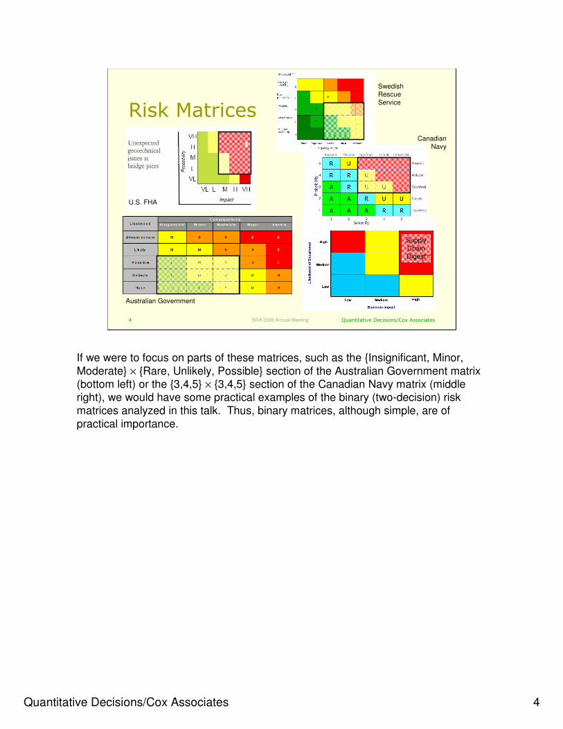
Risk Matrices
U.S. FHA
Australian Government
Swedish Rescue
Service
Canadian Navy
Supply Chain Digest
These are typical. There are many other things also called “risk matrices,” but we
are not concerned with them here.
Apart from immaterial changes, such as interchanging rows for columns or
reversing the orders of rows or columns, all the illustrated risk matrices give color-
coded actions or assessments of risk for combinations of probability/likelihood and impact/consequence/severity.
The last one (bottom right) is clearly suboptimal by assigning high risk to the (Low,
High) cell but only medium risk to the (Medium, High) cell. This talk addresses a
subtler problem: assuming a risk matrix has been correctly colored, just how should it determine which row and column any prospect belongs in? This is a classification
problem.
Note that all these examples are square (having equal numbers of rows and columns). This is typical and, as we will see, it is appropriate: non-square matrices
are unnecessary and redundant.
Accessed via a Google Images search for “risk matrix:”
Unexpected geotechnical issues (Federal (US) Highway Administration)
http://international.fhwa.dot.gov/riskassess/images/figure_12.cfm
Generic risk (Australian Government Department of the Prime Minister and Cabinet)
Quantitative Decisions/Cox Associates 4
Quantitative Decisions/Cox Associates4 SRA 2008 Annual Meeting
Risk Matrices
U.S. FHA
Australian Government
Swedish Rescue
Service
Canadian Navy
Supply Chain Digest
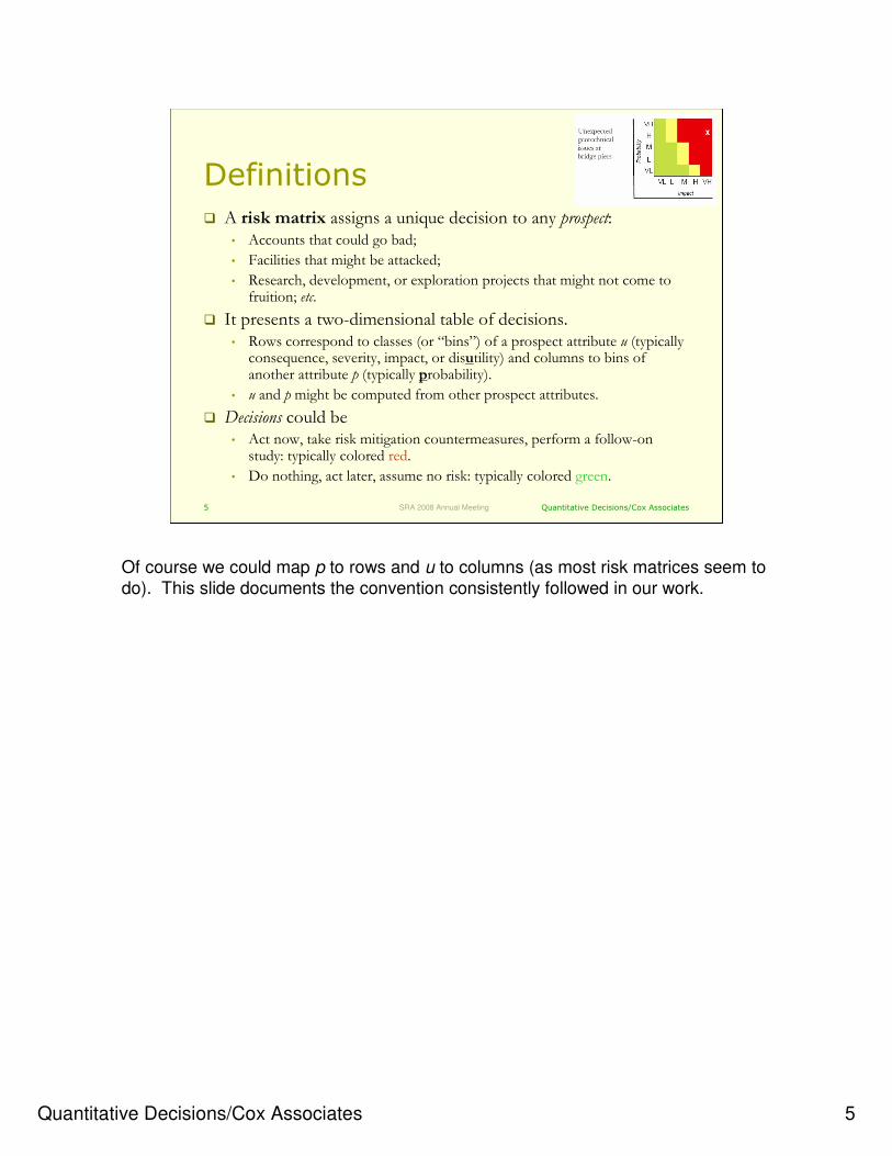
If we were to focus on parts of these matrices, such as the {Insignificant, Minor,
Moderate} × {Rare, Unlikely, Possible} section of the Australian Government matrix (bottom left) or the {3,4,5} × {3,4,5} section of the Canadian Navy matrix (middle right), we would have some practical examples of the binary (two-decision) risk
matrices analyzed in this talk. Thus, binary matrices, although simple, are of
practical importance.
Quantitative Decisions/Cox Associates 5
Quantitative Decisions/Cox Associates5 SRA 2008 Annual Meeting
Definitions
� A risk matrix assigns a unique decision to any prospect:• Accounts that could go bad;
• Facilities that might be attacked;
• Research, development, or exploration projects that might not come to fruition; etc.
� It presents a two-dimensional table of decisions.• Rows correspond to classes (or “bins”) of a prospect attribute u (typically
consequence, severity, impact, or disutility) and columns to bins of another attribute p (typically probability).
• u and p might be computed from other prospect attributes.
� Decisions could be• Act now, take risk mitigation countermeasures, perform a follow-on
study: typically colored red.
• Do nothing, act later, assume no risk: typically colored green.
Of course we could map p to rows and u to columns (as most risk matrices seem to
do). This slide documents the convention consistently followed in our work.
Quantitative Decisions/Cox Associates 6
Quantitative Decisions/Cox Associates6 SRA 2008 Annual Meeting
Uncovering the Detail
Pêches et OcéansCanada
Harvard Business Review (From a consultant’s white paper)
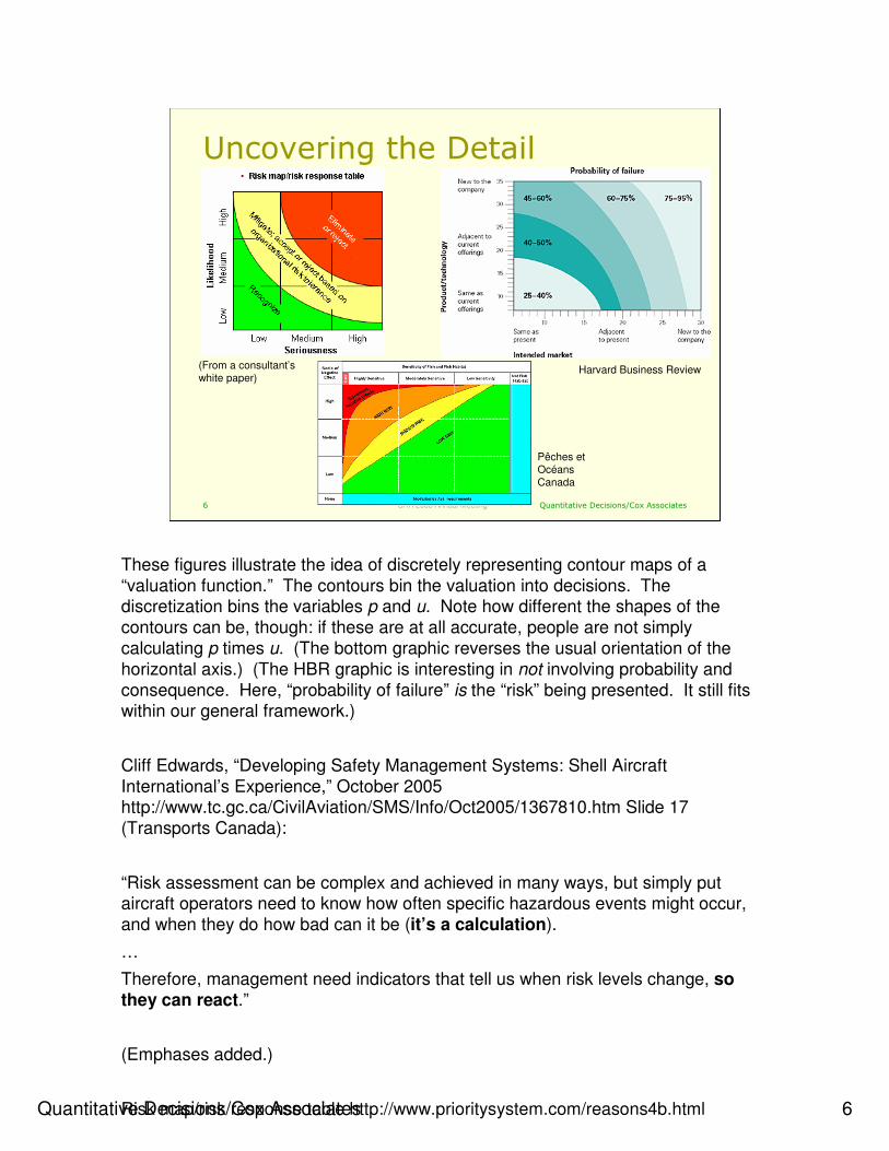
These figures illustrate the idea of discretely representing contour maps of a
“valuation function.” The contours bin the valuation into decisions. The discretization bins the variables p and u. Note how different the shapes of the
contours can be, though: if these are at all accurate, people are not simply
calculating p times u. (The bottom graphic reverses the usual orientation of the
horizontal axis.) (The HBR graphic is interesting in not involving probability and
consequence. Here, “probability of failure” is the “risk” being presented. It still fits within our general framework.)
Cliff Edwards, “Developing Safety Management Systems: Shell Aircraft
International’s Experience,” October 2005 http://www.tc.gc.ca/CivilAviation/SMS/Info/Oct2005/1367810.htm Slide 17
(Transports Canada):
“Risk assessment can be complex and achieved in many ways, but simply put aircraft operators need to know how often specific hazardous events might occur,
and when they do how bad can it be (it’s a calculation).
…
Therefore, management need indicators that tell us when risk levels change, so they can react.”
(Emphases added.)
Risk map/risk response table http://www.prioritysystem.com/reasons4b.html

Quantitative Decisions/Cox Associates 7
Quantitative Decisions/Cox Associates7 SRA 2008 Annual Meeting
Risk Matrices Are DiscreteApproximations
� Their creators clearly conceive of risk matrices as discrete
representations of functional relationships.
� Thus,
• Columns bin the values of p at breakpoints x0 (the smallest possible value of p), x1, x2, …, xn (the largest possible value).
• Rows bin the values of u at breakpoints ym < ym-1 < ym-2 < … < y0.
• Risk is determined by a function v(p,u): the valuation function. (Often p and u can be expressed so that v(p,u) = pu: “risk is probability times consequence.” However, p does not need to be probability, nor does uhave to be consequence, and our theory handles a large class of valuation functions besides pu.)
• Decisions are intervals of risk (z0,z1], (z1,z2], …, (zL-1,zL].
The reversed indexing of the y’s makes the row and column indexes behave in the
conventional manner for matrix indexes: rows go from top to bottom, columns from left to right. This makes the Zig-Zag equations (q.v. infra) a little simpler to write
down systematically, too.

Quantitative Decisions/Cox Associates 8
Quantitative Decisions/Cox Associates8 SRA 2008 Annual Meeting
Notation
... xj -1 xj ...
...
yi
yi -1
...
a ij
u axis
p axis
prospect (p,u)
Bin (yi, yi-1] for u:
yi < u ≤ yi-1.
Bin (xj-1, xj] for p:
xj-1 < p ≤ xj.
row i
co
lum
n j
The decision for prospect (p,u)
is shown here as aij. We talk
about it generically as a colorranging from green through red.
The notation aij is not used again in this talk.
Quantitative Decisions/Cox Associates 9
Quantitative Decisions/Cox Associates9 SRA 2008 Annual Meeting
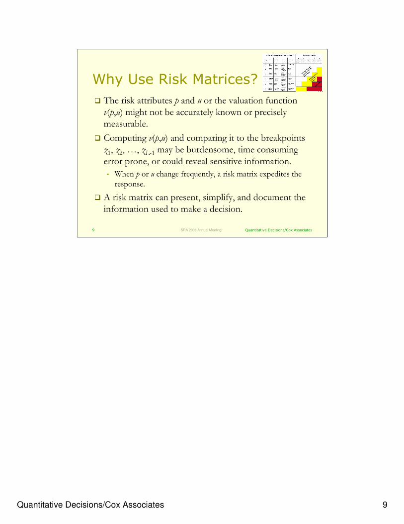
Why Use Risk Matrices?
� The risk attributes p and u or the valuation function v(p,u) might not be accurately known or precisely measurable.
� Computing v(p,u) and comparing it to the breakpoints z1, z2, …, zL-1 may be burdensome, time consuming error prone, or could reveal sensitive information.
• When p or u change frequently, a risk matrix expedites the
response.
� A risk matrix can present, simplify, and document the information used to make a decision.

Quantitative Decisions/Cox Associates 10
Quantitative Decisions/Cox Associates10 SRA 2008 Annual Meeting
Problems with Risk Matrices
� Binning (classifying into categories) the variables p and u almost always loses some information that may be needed for correct decision making.
� This causes the risks of some pairs of prospects to be ranked incorrectly.• It is possible for decisions made with them to be worse than random! (LA
Cox Jr, What’s Wrong with Risk Matrices, Risk Analysis 28(2), 2008).
� An error will occur when a prospect with attributes (p,u) falls into a cell whose color is not the correct one for the “true” risk v(p,u). We call these the “bad” prospects for the risk matrix.• “Gray” cells by definition contain both good and bad prospects.
� How bad can the errors get in actual use?
Quantitative Decisions/Cox Associates 11
Quantitative Decisions/Cox Associates11 SRA 2008 Annual Meeting
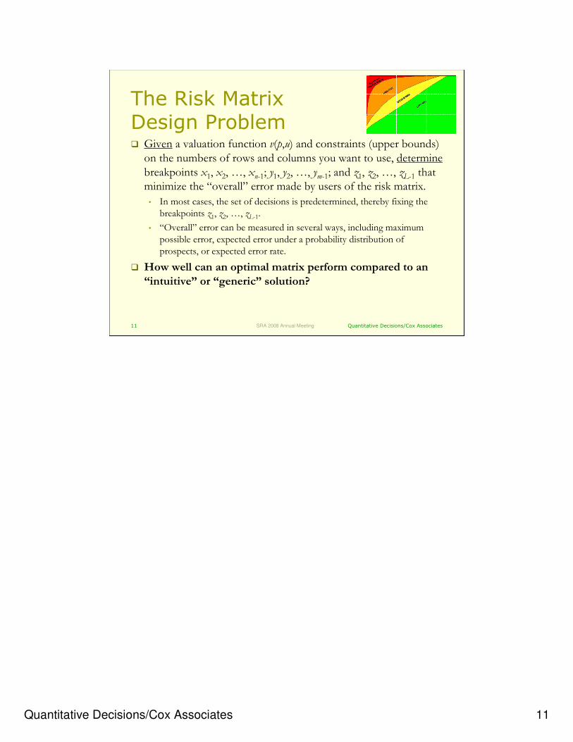
The Risk Matrix Design Problem� Given a valuation function v(p,u) and constraints (upper bounds)
on the numbers of rows and columns you want to use, determine
breakpoints x1, x2, …, xn-1; y1, y2, …, ym-1; and z1, z2, …, zL-1 that minimize the “overall” error made by users of the risk matrix.
• In most cases, the set of decisions is predetermined, thereby fixing the breakpoints z1, z2, …, zL-1.
• “Overall” error can be measured in several ways, including maximum possible error, expected error under a probability distribution of prospects, or expected error rate.
� How well can an optimal matrix perform compared to an
“intuitive” or “generic” solution?
Quantitative Decisions/Cox Associates 12
Quantitative Decisions/Cox Associates12 SRA 2008 Annual Meeting
Theory and Results
The Case of Binary Risk Matrices

Quantitative Decisions/Cox Associates 13
Quantitative Decisions/Cox Associates13 SRA 2008 Annual Meeting
Preliminaries� Re-express p and u so they both lie in the interval [0, 1].
• There is no loss of generality: ultimately both variables will be binned anyway.
� Assume v(p,u) is strictly increasing in both arguments in the interior of its domain (i.e., (0,1) × (0,1)).• This is natural: anything else probably doesn’t qualify as a valuation function.
� A binary (two-decision) problem divides prospects into “green” ones where v(p,u) ≤ k and “red” ones where v(p,u) > k. (k is known as “acceptable risk.”)• The threshold k is fixed. It determines the decision curve {(p,u) : v(p,u) = k}.
� Adopt a cost function C(p,u,d). The cost is that of making decision d for prospect (p,u). Often, C will indicate error or the size of the error.
• When the decision is the correct one, the cost is zero.
• E.g., relative risk is C(p,u,d) = |v(p,u) – k|. Indicator risk is C(p,u,d) = 1.
� Optionally specify a probability (or frequency) distribution Φ for the prospects.
• E.g., the uniform distribution dΦ = dpdu.
The re-expression should be strictly monotonic, of course.
The interpretation of k is unimportant. Presumably, though, red decisions correspond to “more risk”
than green ones. When we quantify “risk” with a valuation function, there must be some threshold
distinguishing red from green: that’s k.
Using a cost function does not complicate the theory, yet makes it applicable in a wider variety of
circumstances. Generally, the cost will depend on the decision made (d) and the prospect’s
attributes (p,u). When d is the correct decision for the prospect, we assign zero cost. Otherwise it is
positive. This generality allows us to cope with situations where there can be a wide spectrum of
consequences of erroneous action, ranging (say) from “it’s the wrong decision, but little harm is done”
to “it would be a disaster to make decision d for prospect (p,u) when the correct decision is d ’ ≠ d.”
Note that the distribution Φ is written in terms of the re-expressed variables. Thus, it most cases it’s
not likely to be uniform. We nevertheless use the uniform distribution to simplify calculations and
illustrate the theory. (One could re-express p and u to make the distribution uniform, or
approximately so, with the consequence that the domain of analysis would no longer be the unit
square. That does not affect our theory. Thus, analysis of the uniform distribution may be of more
general utility than first appears.)

Quantitative Decisions/Cox Associates 14
Quantitative Decisions/Cox Associates14 SRA 2008 Annual Meeting
Two Kinds of Problems
� The minimax problem is to optimize the worst cost that can be incurred in using the risk matrix.
� The expected cost (or expected loss) problem is to optimize the average cost incurred in using the risk matrix.• This requires one to specify the frequencies (or probabilities) with which
the prospects will occur.
� For either problem,• Use indicator risk C(p,u,d) = 1 to measure error rates.
• We use relative risk C(p,u,d) = |v(p,u) – k| to account for the degree of error as well as its occurrence.
• Generally, the cost should increase or at least stay the same as the difference between the risk matrix’s prescription and the true decision increases. We solve the problem in this most general setting.

Quantitative Decisions/Cox Associates 15
Quantitative Decisions/Cox Associates15 SRA 2008 Annual Meeting
Binary Risk Matrices
� Binary risk matrices have two colors only: red and green.
� Understanding them is a key step towards a general theory of optimal risk matrix design.
Műnchener Rűck Munich Re Group
Although binary risk matrices to not appear much in practice, they are an important
class of examples. As pointed out earlier, binary matrices do appear as blocks within actual risk matrices. Thus, it’s essential to understand them before moving
on to the most general situation.
This is a rare example of a risk matrix that does not graduate from green to red!
(This is really a 3 by 3 matrix, not a 4 by 4 one: the right two columns are identical
and so are the bottom two rows. The same information and the same decisions can
be presented by merging the right columns and the bottom rows. Better: given that
you want to devote four columns and rows to presenting this information, you could perform those merges and then reposition the breakpoints, inserting a new one, and
produce a 4 by 4 risk matrix that provides more accurate information about the
proper decision.)
“Example of a Risk Matrix” (Munchener Ruck Munich Re Group)
http://www.munichre.com/en/ts/entrepreneurial_risks/business_continuity_planung/g
raphic_example_of_a_risk_matrix.aspx

Quantitative Decisions/Cox Associates 16
Quantitative Decisions/Cox Associates16 SRA 2008 Annual Meeting
Choosing the Right Decisions
� After binning the variables, you can go cell by cell through the matrix to pick the decision that minimizes the cell’s cost.• When all prospects in the cell have the same
color, give the cell that color (obviously).
• Otherwise
� In the minimax problem, consider the worst prospect for each possible cell color. Choose the color that minimizes this worst case.
� In the expected cost problem, choose the color that minimizes the expected cost over the cell.
� Thus, the problems of choosing breakpoints and coloring the cells are decoupled.
However we color this gray cell, the worst costs will be incurred at the two corner cells marked.
In solving the expected cost problem, we have to integrate the
cost over the upper half of the cell (if it’s colored green) or over the lower half (if it’s colored red).
The curve in the illustration graphs the decision curve. By definition, the gray cells
are the ones it passes through. Only one of them is shown.

Quantitative Decisions/Cox Associates 17
Quantitative Decisions/Cox Associates17 SRA 2008 Annual Meeting
Sweeping through a Strip� Focus on one column as you vary one y-breakpoint.
config33a new.ggb
The cost of this
cell goes up …
while the cost of this
cell goes down.
We prove there is a unique point in the sweep where the sum of the two
costs is smallest.
The colored dots mark curvilinear triangles containing bad prospects. E.g., the cell for the green dot (at
the left) will necessarily be colored red, but this prospect—lying below the decision curve—is green.
The left image shows the situation just before the sweep line (at Y2) descends
through the decision curve at the X2 breakpoint. Until it does, there is no question about how to color the Y1Y2, X2X3 cell at the top: it’s not a gray cell.
In the middle, the sweep line now bounds gray cells both above and below. They
both potentially contribute to the overall cost. Our assumptions about the valuation and cost function imply the upper cell must be red and the lower one green. Thus,
the curvilinear triangles bounded by the decision curve with apexes at P22 and P32
contain the bad prospects.
The bottom shows the point just before the sweep line passes below the decision curve at the X3 breakpoint. Below this, the bottom cell will be green, not gray, and
there’s no more analysis to be done.
Of course this technique also works for horizontal sweeps that vary a p breakpoint.

Quantitative Decisions/Cox Associates 18
Quantitative Decisions/Cox Associates18 SRA 2008 Annual Meeting
The Key Idea
� At any critical point, the infinitesimal increase in cost contributed by the green (left) line segment balances the infinitesimal decrease in cost contributed by the red
(right) line segment.
The green segment consists of bad points (green prospects colored red by the
matrix) swept out during one instant. The red segment consists of bad points (red prospects colored green by the matrix) also swept out. As the sweep line
descends, the green segment increases and the red segment decreases. The
assumptions about the valuation and cost functions imply the contribution of the
green segment to the overall cost is growing (well, not decreasing) while the
contribution of the red segment is shrinking (not increasing).
When the distribution function (for expected cost) is nonzero, there must be a
unique intermediate point along the sweep where the overall cost is minimized. For
minimax loss, we arrive at the same conclusion (through slightly different reasoning).

Quantitative Decisions/Cox Associates 19
Quantitative Decisions/Cox Associates19 SRA 2008 Annual Meeting
Result 1: Use Square Matrices
� Make the matrix as square as possible (that is, m and nshould be equal or differ by one).
• If not, there will be neighboring rows (or columns) that can
be combined without any increase in overall cost.
No matter how we vary y2between y1 and y3, the row
of cells between y1 and y2must always be colored the same as the row of cells
between y2 and y3. Thus, y2is unnecessary.
This situation always happens when there are
more rows than columns+1.
(The blue dots near Y0 and Y2 are used in the software to set the locations of the
breaklines.)
Quantitative Decisions/Cox Associates 20
Quantitative Decisions/Cox Associates20 SRA 2008 Annual Meeting
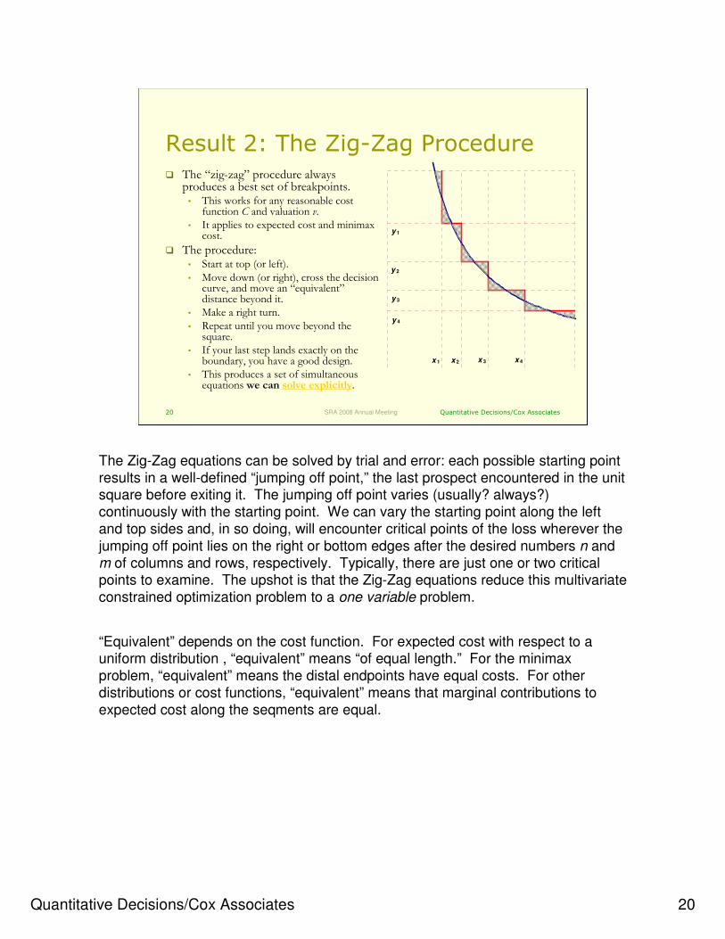
Result 2: The Zig-Zag Procedure� The “zig-zag” procedure always
produces a best set of breakpoints.• This works for any reasonable cost
function C and valuation v.• It applies to expected cost and minimax
cost.
� The procedure:• Start at top (or left).
• Move down (or right), cross the decision curve, and move an “equivalent” distance beyond it.
• Make a right turn.
• Repeat until you move beyond the square.
• If your last step lands exactly on the boundary, you have a good design.
• This produces a set of simultaneous equations we can solve explicitly.
x 4x 3x 2x 1
y 1
y 2
y 3
y 4
The Zig-Zag equations can be solved by trial and error: each possible starting point
results in a well-defined “jumping off point,” the last prospect encountered in the unit square before exiting it. The jumping off point varies (usually? always?)
continuously with the starting point. We can vary the starting point along the left
and top sides and, in so doing, will encounter critical points of the loss wherever the
jumping off point lies on the right or bottom edges after the desired numbers n and
m of columns and rows, respectively. Typically, there are just one or two critical points to examine. The upshot is that the Zig-Zag equations reduce this multivariate
constrained optimization problem to a one variable problem.
“Equivalent” depends on the cost function. For expected cost with respect to a uniform distribution , “equivalent” means “of equal length.” For the minimax
problem, “equivalent” means the distal endpoints have equal costs. For other
distributions or cost functions, “equivalent” means that marginal contributions to
expected cost along the seqments are equal.
Quantitative Decisions/Cox Associates 21
Quantitative Decisions/Cox Associates21 SRA 2008 Annual Meeting
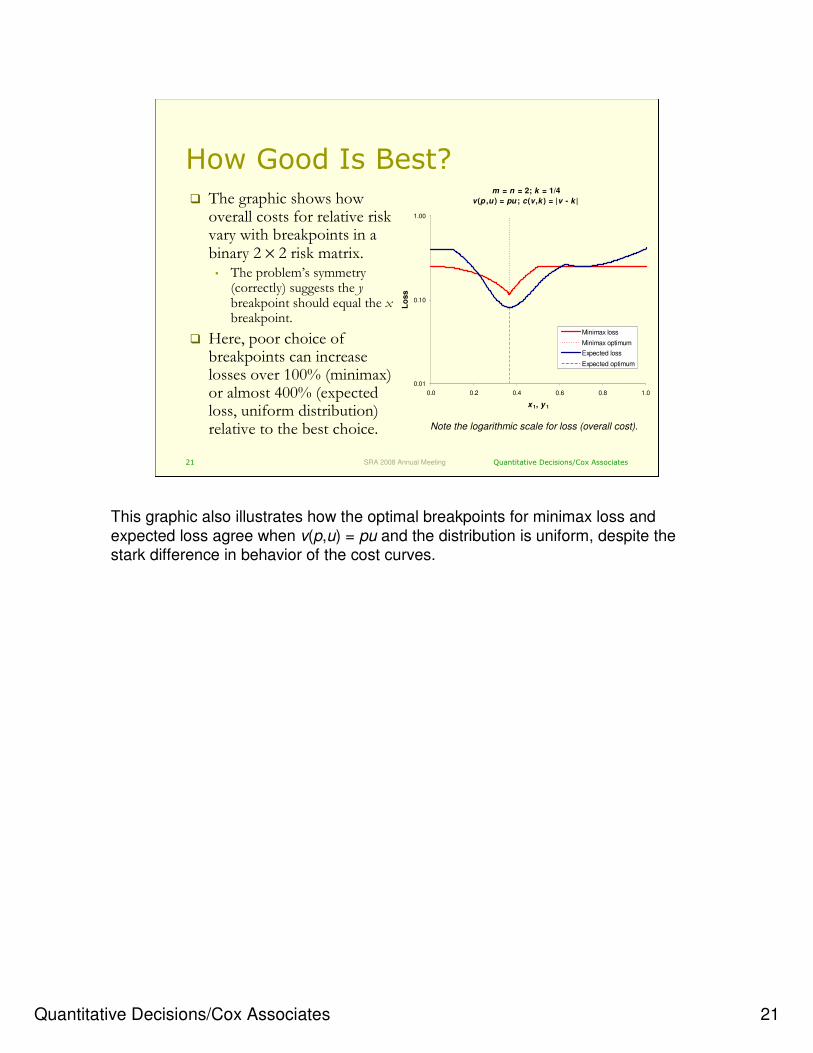
How Good Is Best?
� The graphic shows how overall costs for relative risk vary with breakpoints in a binary 2 × 2 risk matrix.• The problem’s symmetry
(correctly) suggests the ybreakpoint should equal the xbreakpoint.
� Here, poor choice of breakpoints can increase losses over 100% (minimax) or almost 400% (expected loss, uniform distribution) relative to the best choice.
m = n = 2; k = 1/4
v(p ,u ) = pu ; c(v ,k ) = |v - k |
0.01
0.10
1.00
0.0 0.2 0.4 0.6 0.8 1.0
x 1, y 1L
oss
Minimax loss
Minimax optimum
Expected loss
Expected optimum
Note the logarithmic scale for loss (overall cost).
This graphic also illustrates how the optimal breakpoints for minimax loss and
expected loss agree when v(p,u) = pu and the distribution is uniform, despite the stark difference in behavior of the cost curves.
Quantitative Decisions/Cox Associates 22
Quantitative Decisions/Cox Associates22 SRA 2008 Annual Meeting
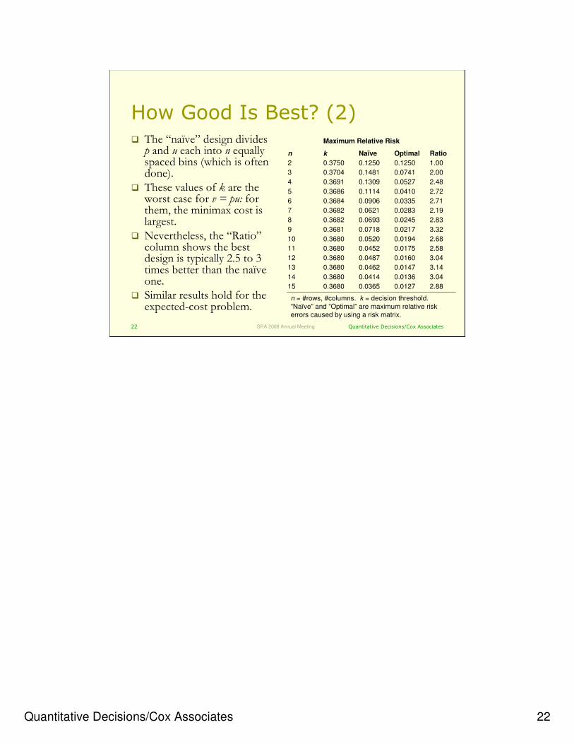
How Good Is Best? (2)� The “naïve” design divides
p and u each into n equally spaced bins (which is often done).
� These values of k are the worst case for v = pu: for them, the minimax cost is largest.
� Nevertheless, the “Ratio” column shows the best design is typically 2.5 to 3 times better than the naïve one.
� Similar results hold for the expected-cost problem.
Maximum Relative Risk
n k Naïve Optimal Ratio
2 0.3750 0.1250 0.1250 1.00
3 0.3704 0.1481 0.0741 2.00
4 0.3691 0.1309 0.0527 2.48
5 0.3686 0.1114 0.0410 2.72
6 0.3684 0.0906 0.0335 2.71
7 0.3682 0.0621 0.0283 2.19
8 0.3682 0.0693 0.0245 2.83
9 0.3681 0.0718 0.0217 3.32
10 0.3680 0.0520 0.0194 2.68
11 0.3680 0.0452 0.0175 2.58
12 0.3680 0.0487 0.0160 3.04
13 0.3680 0.0462 0.0147 3.14
14 0.3680 0.0414 0.0136 3.04
15 0.3680 0.0365 0.0127 2.88
n = #rows, #columns. k = decision threshold.“Naïve” and “Optimal” are maximum relative risk errors caused by using a risk matrix.
Quantitative Decisions/Cox Associates 23
Quantitative Decisions/Cox Associates23 SRA 2008 Annual Meeting
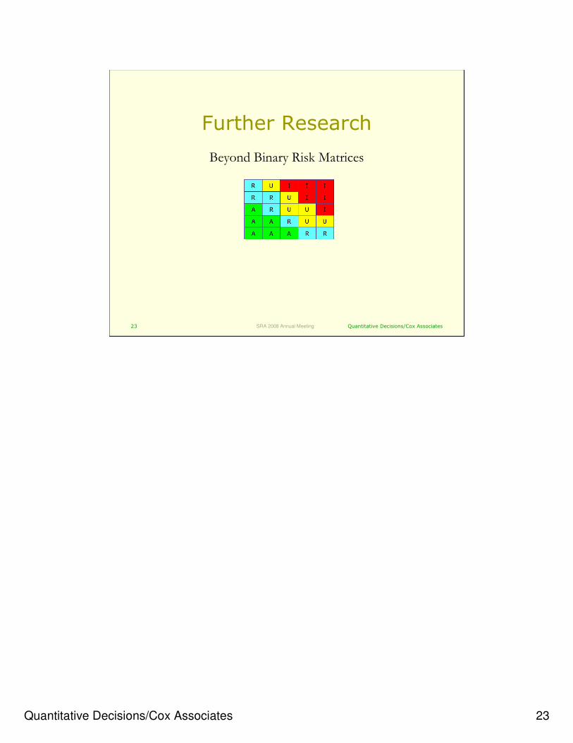
Further Research
Beyond Binary Risk Matrices

Quantitative Decisions/Cox Associates 24
Quantitative Decisions/Cox Associates24 SRA 2008 Annual Meeting
What Next?
� What can we say about more than two decisions?• The strip sweep analysis still works.
• The Zig-Zag procedure does not easily extend to more than two decisions because of interactions between strips.
• It is unlikely we will find any simple, clear characterization of all optimal risk matrices.
� What can we say about arbitrary probability distributions of prospects?• Not much, unless we make strong assumptions.
� Nevertheless, our results for the binary case suggest significant improvements over intuitive or naïve designs are possible.• The Zig-Zag procedure applied independently to the L-1 cutoffs for an
L-decision matrix might be a good heuristic guide in many cases.
This seems pretty negative, but it’s a realistic assessment: the problem gets really
messy with three or more decisions. The next step might be to run some numerical experiments with ternary risk matrices as a guide to what to expect from a
theoretical analysis (if one is even possible).

Quantitative Decisions/Cox Associates 25
Quantitative Decisions/Cox Associates25 SRA 2008 Annual Meeting
If You Must Create Risk Matrices…
� Consider using the Zig-Zag procedure to help determine cutoffs for p and u in your risk matrices.
� More generally, evaluate the potential effects of a risk matrix in terms of the maximum error or expected error incurred by its users.
� If your analysis suggests the error rates are unacceptable, you can• Increase the numbers of rows and columns (and repeat the
Zig-Zag procedure) or
• Provide quantitative decision procedures (formulas) or software in place of a risk matrix.

Quantitative Decisions/Cox Associates 26
Quantitative Decisions/Cox Associates26 SRA 2008 Annual Meeting
Supporting you and solving your problems with maps, numbers, and analyses.
www.quantdec.com
QD and CA
Superior business decisions through better data analysis.
www.cox-associates.com

Quantitative Decisions/Cox Associates 27
Quantitative Decisions/Cox Associates27 SRA 2008 Annual Meeting
Finding the Best Breakpoints
� The overall cost of the design, given that we have selected the
best color for each cell, is a function of n+m–2 variables subject to the constraints 0<x1<x2 …<xn-1<1>y1>y2>…>ym-1>0.
� For the minimax problem the cost is not differentiable (vide the
red curve) so we have to be careful about using Calculus.
� Nevertheless, we can use the fundamental idea of looking for the
best design at critical points where independent small changes in
any variable no longer improve the cost.
� Changing any variable causes changes in the strips of cells through which it passes. Therefore, we study how the cost
changes as a breakpoint sweeps across one strip.
0.10
Lo
ss
The graphic is explained in a later slide (“How Good Is Best?”).
The cost is a not-very-nice function to be optimized subject to a set of linear
constraints.
This approach to the problem (a strip sweep) looks natural and obvious. There are plenty of other natural and obvious approaches, though, and it took a while to arrive
at this one!
Quantitative Decisions/Cox Associates 28
Quantitative Decisions/Cox Associates28 SRA 2008 Annual Meeting
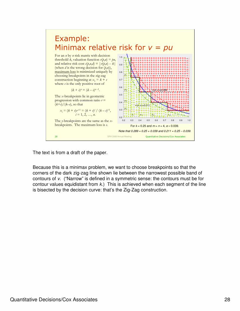
Example:Minimax relative risk for v = pu
0.2
0.3
0.4
0.5
0.6
0.7
0.8
0.9
1.0
0.2 0.3 0.4 0.5 0.6 0.7 0.8 0.9 1.0
x 1 x 2 x 3 x 4
y 1
y 2
y 3
y 4
v (p ,u )=0.289
v (p ,u )=0.211
For an n by n risk matrix with decision threshold k, valuation function v(p,u) = pu, and relative risk cost c(p,u,d) = |v(p,u) – k| (when d is the wrong decision for (p,u)), maximum loss is minimized uniquely by choosing breakpoints in the zig-zag construction beginning at x1 = k + ewhere e is the only positive root of
(k + e)n = (k – e)n –1.
The x-breakpoints lie in geometric progression with common ratio r = (k+e)/(k–e), so that
xi = (k + e)r i-1 = (k + e)i / (k – e)i-1,i = 1, 2, …, n.
The y-breakpoints are the same as the x-breakpoints. The maximum loss is e. For k = 0.25 and m = n = 4, e ≈ 0.039.
Note that 0.289 = 0.25 + 0.039 and 0.211 = 0.25 – 0.039.
The text is from a draft of the paper.
Because this is a minimax problem, we want to choose breakpoints so that the
corners of the dark zig-zag line shown lie between the narrowest possible band of
contours of v. (“Narrow” is defined in a symmetric sense: the contours must be for
contour values equidistant from k.) This is achieved when each segment of the line is bisected by the decision curve: that’s the Zig-Zag construction.