Chapter 4

Optimizing Power @ Design Time – Circuit-Level Techniques

Jan M. Rabaey

Optimizing Power @ Design Time

Circuits

Dejan MarkovicBorivoje Nikolic

Slide 4.1

Chapter Outline

Optimization framework for energy–delay trade-offDynamic-power optimization – Multiple supply voltages– Transistor sizing– Technology mapping

Static-power optimization– Multiple thresholds– Transistor stacking

Slide 4.2

Energy/Power Optimization Strategy

For given function and activity, an optimal operation point can be derived in the energy–performance spaceTime of optimization depends upon activity profile Different optimizations apply to active and static power

Fixed Activity

Variable Activity

No Activity – Standby

ActiveDesign time Run time Sleep

Static

Slide 4.3

Maximize throughput for given energy orMinimize energy for given throughput

Delay

design

Emax

DmaxDmin

Energy/op

Emin

Energy–Delay Optimization and Trade-off

Trade-off space

Other important metrics: Area, Reliability, Reusability

Unoptimized

Slide 4.4

The Design Abstraction Stack

Logic/RT

(Micro-)Architecture

Software

Circuit

Device

System/Application

Thi

s C

hapt

er

A very rich set of design parameters to consider!It helps to consider options in relation to their abstraction layer

sizing, supply, thresholds

logic family, standard cell versus custom

Parallel versus pipelined, general purpose versus application-specific

Bulk versus SOI

Choice of algorithm

Amount of concurrency

Slide 4.5

Architecture

Micro-Architecture

Circuit (Logic & FFs)

Optimization Can/Must Span Multiple Levels

Design optimization combines top-down and bottom-up: “meet-in-the-middle”

Slide 4.6

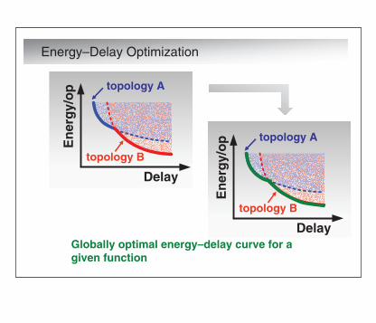
topology A

DelayE

ner

gy/

op

Globally optimal energy–delay curve for a given function

Energy–Delay Optimization

topology B

topology A

topology B

Delay

En

erg

y/o

p

Slide 4.7

Some Optimization Observations

∂E/∂A∂D/∂A A=A0

SA =

SB

SA

f(A0,B)

f(A,B0)

Delay

En

erg

y

D0

(A0,B0)

Energy–Delay Sensitivities

[Ref: V. Stojanovic, ESSCIRC’02]

Slide 4.8

ΔE = SA · (−ΔD) + SB · ΔD

On the optimal curve, all sensitivities must be equal

Finding the Optimal Energy–Delay Curve

f(A0,B)

f(A,B0)

Delay

En

erg

y

D0

(A0,B0)

ΔD

f(A1,B)

Pareto-optimal:the best that can be achieved without disadvantaging at least one metric.

Slide 4.9

Reducing voltages– Lowering the supply voltage (VDD) at the expense of clock speed– Lowering the logic swing (Vswing)

Reducing transistor sizes (CL )– Slows down logic

Reducing activity (α)– Reducing switching activity through transformations– Reducing glitching by balancing logic

fVVCP DDswingLactive ⋅⋅⋅⋅~DDswingLactive VVCα

αE ⋅⋅⋅~

Reducing Active Energy @ Design Time

Slide 4.10

Downsizing and/or lowering the supply on the critical path lowers the operating frequencyDownsizing non-critical paths reduces energy for free, but– Narrows down the path–delay distribution– Increases impact of variations, impacts robustness

tp(path)

# of

pat

hs

targetdelay

# of

pat

hs

targetdelay

Observation

tp(path)

Slide 4.11

topology A

topology B

DelayE

ner

gy/

op

Reference case– Dmin sizing @ VDD max, VTH ref

minimize Energy (VDD, VTH, W )subject to Delay (VDD, VTH, W ) D≤ con

ConstraintsVDD min < VDD < VDD max

VTH min < VTH< VTH max

Wmin < W

Circuit Optimization Framework

[Ref: V. Stojanovic, ESSCIRC’02]

Slide 4.12

i i +1

CwCiC γi Ci +1

Optimization Framework: Generic Network

VDD i +1VDD i

Gate in stage i loaded by fan-out (stage i +1)

Slide 4.13

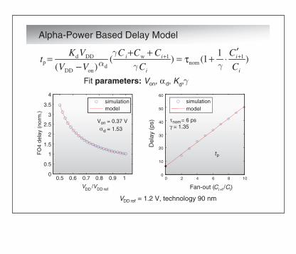
Fit parameters: Von, αd, K ,d γ

Alpha-Power Based Delay Model

VDD ref = 1.2 V, technology 90 nm

)1

1()()(

11

i

inom

i

iwi

onDD

DDd

C

C

C

CCCγγ γτ

VV

VKtp

++ ′⋅+=++

−=

0 2 4 6 8 100

10

20

30

40

50

60

Fan-out (Ci +1/Ci)

Del

ay (

ps)

tp

0.5 0.6 0.7 0.8 0.9 1 0

0.5

1

1.5

2

2.5

3

3.5

4

VDD

/VDD ref

FO

4 de

lay

(nor

m.)

Von = 0.37 Vαd = 1.53

simulationmodel

τnom= 6 psγ = 1.35

simulationmodel

αd

Slide 4.14

Parasitic delay pi –

≈

depends upon gate topology

Electrical effort f i S i+1/S i

Logical effort gi – depends upon gate topology

Effective fan-out hi = fi gi

For Complex Gates

Combined with Logical-Effort Formulation

)( iiinom

gfptp τ γ+=

[Ref: I. Sutherland, Morgan-Kaufman’99]

Slide 4.15

= energy consumed by logic gate i

Dynamic Energy

i i +1

CwCiCi Ci+1

VDD,i +1VDD,i

iiiiwiiei

iDDiiiDDiwidyn

SSCCCfSKC

VfCV γγ

γ

CCCE

//)(

)()(

11

2,

2,1

++

+

′=+=′=

⋅′+=⋅++=

)( 2,

21, iDDiDDiei VVSKE += −

γ

Slide 4.16

∞ for equal h

(Dmin)

max at VDD(max)

(Dmin)

Depends on Sensitivity (∂E /∂D)

Optimizing Return on Investment (ROI)

Gate Sizing

Supply Voltage

)( 1−−−=

∂∂

∂∂

iinom

i

i

i

hh

E

τ

α

SD

SE

DD

ond

DD

on

DD

DD

V

VV

V

D

E

VD

VE

+−

−⋅⋅−=

∂∂

∂∂

1

)1(2

Slide 4.17

Properties of inverter chain– Single path topology– Energy increases geometrically from input to output

Example: Inverter Chain

CL

1

S1 = 1 S2 … SNS3

Goal– Find optimal sizing S = [S1, S2, …, SN ], supply voltage, and

buffering strategy to achieve the best energy–delay trade-off

Slide 4.18

Variable taper achieves minimum energy

[Ref: Ma, JSSC’94]

Inverter Chain: Gate Sizing

1 2 3 4 5 6 70

5

10

15

20

25

stage

effe

ctiv

e fa

n-ou

t, h

0%

1%

10%

30%

Dinc

= 50%nomopt

1

21

112

21

−

−

+−

−∝

⋅⋅⋅−=μ τ

+ μ⋅=

ii

iS

Snom

DDe

i

iii

hh

EF

FVK

S

SSS

Slide 4.19

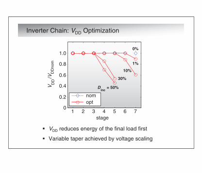
VDD reduces energy of the final load first

Variable taper achieved by voltage scaling

Inverter Chain: VDD Optimization

1 2 3 4 5 6 70

0.2

0.4

0.6

0.8

1.0

stage

VD

D/V

DD

nom

0%

1%

10%

30%

Dinc

= 50%

nomopt

Slide 4.20

Parameter with the largest sensitivity has the largest potential for energy reductionTwo discrete supplies mimic per-stage V DD

Inverter Chain: Optimization Results

500 10 20 30 400

20

40

60

80

100

incD (%)

ener

gy r

educ

tion

(%)

0 10 20 30 40 500

0.2

0.4

0.6

0.8

1.0

Dinc

(%)

Sen

sitiv

ity (

norm

)

cVDD

SgV DD

2V DD

Slide 4.21

Tree adder– Long wires– Reconvergent paths– Multiple active outputs

(A0, B0)

Example: Kogge–Stone Tree Adder

Cin

(A15, B15)

S0

S15

[Ref: P. Kogge, Trans. Comp’73]

Slide 4.22

sizing: E (–54%)D = 10%

referenceD = D

Dual VDD : E (–27%)D = 10%

Tree Adder: Sizing vs. Dual-VDD Optimization

Reference design: all paths are critical

Internal energy ⇒ S more effective than V DD– S: E(–54%), Dual VDD: E(–27%) at D inc = 10%

incmin inc

10080604020

ener

gy

bit slice

stage63 47 31 15 0 13

57

9

10080604020

ener

gy

bit slicesta

ge63 47 31 15 0 13

57

9

10080604020

ener

gy

bit slice

stage63 47 31 15 0 1

35

79

Slide 4.23

Tree Adder: Multi-dimensional Search

Can get pretty close to optimum with only two variablesGetting the minimum speed or delay is very expensive

En

erg

y/E

ref

Delay/Dmin

0.4 0.6 0.8 1 1.2 1.4 1.6 1.8 20

0.2

0.4

0.6

0.8

1Reference

S, V DD

VDD, VTH

S, V TH

S, V DD, V TH

Slide 4.24

Block-level supply assignment– Higher-throughput/lower-latency functions are

implemented in higher VDD

– Slower functions are implemented with lower VDD

– This leads to so-called voltage islands with separate supply grids

– Level conversion performed at block boundaries

Multiple supplies inside a block– Non-critical paths moved to lower supply voltage– Level conversion within the block– Physical design challenging

Multiple Supply Voltages

Slide 4.25

V1 = 1.5V, VTH = 0.3V

Using Three VDD’s

+

V2 (V)

V3

(V)

0.4 0.6 0.8 1 1.2 1.4

0.4

0.6

0.8

1

1.2

1.4

V2 (V)V

3 (V)

Po

wer

Red

uct

ion

Rat

io

00.5

11.5

0

0.51

1.50.4

0.5

0.6

0.7

0.8

0.9

1

[Ref: T. Kuroda, ICCAD’02]

Slide 4.26

1.0

0.5

VD

D R

atio

1.0

0.4

0.5 1.0 1.5V1 (V)

P R

atio

V2 /V1

P2 /P1

{ V1, V2 }

V2 /V1

V3 /V1

{ V1, V2, V3 }

0.5 1.0 1.5V1 (V)

P3 /P1

V2 /V1

V3 /V1

V4 /V1

0.5 1.0 1.5V1 (V)

P4 /P1

{ V1, V2, V3, V4 }

Optimum Number of VDDs

The more the number of VDD s the less the power, but the effect saturates

Power reduction effect decreases with scaling of VDD

Optimum V2 /V1 is around 0.7

© IEEE 2001

[Ref: M. Hamada, CICC’01]

Slide 4.27

Two supply voltages per block are optimal

Optimal ratio between the supply voltages is 0.7

Level conversion is performed on the voltage boundary, using a level-converting flip-flop (LCFF)

An option is to use an asynchronous level converter– More sensitive to coupling and supply noise

Lessons: Multiple Supply Voltages

Slide 4.28

i1 o1

VDDHVDDL

VSS

Conventional

VDDH circuit V DDL circuit

i2 o2

V DDH

V DDL

V SS

Shared n-well

VDDH circuit VDDL circuit

Distributing Multiple Supply Voltages

i2 o2

i1 o1

Slide 4.29

V DDH circuit

VDDH V DDL

VSS

n-well isolation

V DDL circuit

(a) Dedicated row

(b) Dedicated region

VDDH Row

VDDH Row

VDDH

RegionVDDL

Region

Conventional

VDDL Row

VDDL Row

Slide 4.30

VDDH circuit

V DDH

VDDL

VSS

Shared n-well

VDDL circuit

(a) Floor plan image

V DDL circuit

V DDH circuit

Shared n-Well

[Shimazaki et al., ISSCC’03]

Slide 4.31

Lower VDD portion is shared“Clustered voltage scaling”

Example: Multiple Supplies in a Block

FF

FF

FF

FFFF

FF

FF

FF

FF

FF

CVS StructureConventional Design

Critical Path

Level-Shifting FF

Critical Path

FF

FF

FF

FF

FF

FF FF

FF

FF

FF

FF

[Ref: M. Takahashi, ISSCC’98]

© IEEE 1998

Slide 4.32

Pulsed Half-Latch versus Master–Slave LCFFsSmaller # of MOSFETs/clock loadingFaster level conversion using half-latch structureShorter D–Q path from pulsed circuit

Level-Converting Flip-Flops (LCFFs)

q

ck

ckb ckclk

level conversion

ckb

ckd q (inv.)

ck

ckclk

level conversion

dmo

mf

sfso db

sfso

MN1 MN2

Master–Slave Pulsed Half-Latch

© IEEE 2003

[Ref: F. Ishihara, ISLPED’03]

Slide 4.33

Dynamic Realization of Pulsed LCFF

Pulsed precharge LCFF (PPR)– Fast level conversion by

precharge mechanism– Suppressed

charge/discharge toggle by conditional capture

– Short D–Q path

Pulsed Precharge Latch

clk

ckd1

qb

clk level conversion

x

db

qb

ckd1

VDDH

VDDH

VDDH

d

xb

IV1

q (inv.)

ck

MN1

MN2

MP1

[Ref: F. Ishihara, ISLPED’03]© IEEE 2003

Slide 4.34

carrygen.

partialsum

gpgen.

5:1MUX

ain

bin

carry

s0/s1

sum

sumb (long loop-back bus)

clk

clock gen.

: V DDH circuit

: V DDL circuit

INV1INV2

0.5 pF

sumsel.

2:1MUX

9:1MUX

logicalunit

9:1MUX

ain0

Case Study: ALU for 64-bit Microprocessor

[Ref: Y. Shimazaki, ISSCC’03]© IEEE 2003

Slide 4.35

sum

keeperpc

sumb

VDDH

VDDL

INV1 INV2

domino level converter (9:1 MUX)

ain0sel(VDDH)

VDDH

VDDL

INV2 is placed near 9:1 MUX to increase noise immunityLevel conversion is done by a domino 9:1 MUX

Low-Swing Bus and Level Converter

[Ref: Y. Shimazaki, ISSCC’03]

© IEEE 2003

Slide 4.36

[Ref: Y. Shimazaki, ISSCC’03]

Single-supplyShared-well(VDDH=1.8 V)E

nerg

y [p

J]

TCYCLE [ns]

Room temperature

200

300

400

500

600

700

800

0.6 0.8 1.0 1.2 1.4 1.6

1.16 GHz

VDDL=1.4 VEnergy:–25.3% Delay :+2.8%

VDDL=1.2 VEnergy:–33.3% Delay :+8.3%

Measured Results: Energy and Delay

© IEEE 2003

Slide 4.37

Practical Transistor Sizing

Continuous sizing of transistors only an option in custom design

In ASIC design flows, options set by available library

Discrete sizing options made possible in standard-cell design methodology by providing multiple options for the same cell– Leads to larger libraries (> 800 cells)– Easily integrated into technology mapping

Slide 4.38

Larger gates reduce capacitance, but are slower

Technology Mapping

a

b

c

slack = 1

d

f

Slide 4.39

(a) Implemented using four-input NAND + INV(b) Implemented using two-input NAND + two-input NOR

Library 1: High-Speed

Technology Mapping

Example: four-input AND

Gatetype

Area (cell unit)

Input cap. (fF)

Average delay (ps)

Average delay (ps)

INV 3 1.8 7.0 + 3.8C L 12.0 + 6.0C L

NAND2 4 2.0 10.3 + 5.3C L 16.3 + 8.8CL

NAND4 5 2.0 13.6 + 5.8C L 22.7 + 10.2CL

NOR2 3 2.2 10.7 + 5.4C L 16.7 + 8.9CL

Library 2: Low-Power

(delay formula: C

(numbers calibrated for 90 nm)L in fF)

Slide 4.40

Technology Mapping – Example

four-input AND (a) NAND4 + INV

(b) NAND2 + NOR2

Area 8 11

HS: Delay (ps) 31.0 + 3.8CL

53.1 + 6.0CL

0.1 + 0.06CL

32.7 + 5.4CL

LP: Delay (ps) 52.4 + 8.9CL

Sw Energy (fF) 0.83 + 0.06CL

Area– Four-input more compact than two-input (two gates vs three gates)

Timing– Both implementations are two-stage realizations– Second-stage INV (a) is better driver than NOR2 (b)– For more complex blocks, simpler gates will show better

performanceEnergy– Internal switching increases energy in the two-input case– Low-power library has worse delay, but lower leakage (see later)

Slide 4.41

Technology mappingGate selectionSizingPin assignment

Logical OptimizationsFactoring

Restructuring

Buffer insertion/deletion

Don’t - care optimization

Gate-Level Trade-offs for Power

Slide 4.42

Logic restructuring to minimize spurious transitions

Buffer insertion for path balancing

Logic Restructuring

01

1

1

0

1

1

1

0

1 1

1

1

1

1

111

2

3

Slide 4.43

Idea: Modify network to reduce capacitance

Caveat: This may increase activity!

pa pb= 0.1; = 0.5; pc = 0.5

Algebraic Transformations Factoring

a

bc

ff

a

a

b

c

p1 = 0.051

p2 = 0.051

p3 = 0.076

p4 = 0.375

p5 = 0.076

Slide 4.44

Energy-efficient design

Joint optimization over multiple design parameters possible using sensitivity-based optimization framework– Equal marginal costs ⇔

Peak performance is VERY power inefficient– About 70% energy reduction for 20% delay penalty– Additional variables for higher energy-efficiency

Two supply voltages in general sufficient; three or more supply voltages only offer small advantage

Choice between sizing and supply voltage parameters depends upon circuit topology

But … leakage not considered so far

Lessons from Circuit Optimization

Slide 4.45

Considering leakage as well as dynamic

power is essential in sub-100 nm

technologies

Leakage is not essentially a bad thing

– Increased leakage leads to improved

performance, allowing for lower supply voltages

– Again a trade-off issue …

Considering Leakage at Design Time

Slide 4.46

Must adapt to process and activity variations

( ) 2

αln

lk sw optd

avg

E EL

K

=

−

Topology Inv Add Dec

(E lk /Esw)opt 0.8 0.5 0.2

Leakage – Not Necessarily a Bad Thing

Optimal designs have high leakage (Elk /Esw 0.5)≈

10–2

10–1

100

101

0

0.2

0.4

0.6

0.8

1

Estatic /Edynamic

Eno

rm

VTHref-180 mV

0.81VDDmax

VTHref-140 mV

0.52VDDmax

Version 1

Version 2

[Ref: D. Markovic, JSSC’04]

© IEEE 2004

Slide 4.47

Switching energy

Leakage energy

with:I0(Ψ): normalized leakage current with inputs in state Ψ

Refining the Optimization Model

210 )( DDedyn VfSKE += →

cycleDDqkT

VV

stat TVeSIEDDdTH

/0 )(

+−

Ψ=

α

λ

γ

Slide 4.48

Using longer transistors– Limited benefit– Increase in active current

Using higher thresholds– Channel doping– Stacked devices– Body biasing

Reducing the voltage!!

Reducing Leakage @ Design Time

Slide 4.49

10% longer gates reduce leakage by 50%Increases switching power by 18% with W/L = constant

Doubling L reduces leakage by 5xImpacts performance

– Attractive when not required to increase W (e.g., memory)

Longer Channels

100 110 120 130 140 150 160 170 180 190 2000.1

0.2

0.3

0.4

0.5

0.6

0.7

0.8

0.9

1.0

Transistor length (nm)

1

2

3

4

5

6

7

8

9

10

90 nm CMOS

Switching energy

Leakage power

Nor

mal

ized

sw

itchi

ng e

nerg

y

Nor

mal

ized

leak

age

pow

er

Slide 4.50

There is no need for level conversion

Dual thresholds can be added to standard design flows– High-VTH and Low-VTH libraries are a standard in sub-0.18 μm

processes– For example: can synthesize using only high-VTH and then simply

swap-in low-VTH cells to improve timing.– Second VTH insertion can be combined with resizing

Only two thresholds are needed per block– Using more than two yields small improvements

Using Multiple Thresholds

Slide 4.51

Three VTH’s

VDD = 1.5 V, VTH.1 = 0.3 V

+

VTH.3(V)

VT

H.2

(V)

0.4 0.6 0.8 1 1.2 1.4

0.4

0.6

0.8

1

1.2

1.4

Lea

kag

e R

edu

ctio

n R

atio

VTH.3(V)

VTH.2 (V )

00.5

11.5

0

11.5

0.5

0

0.2

0.4

0.6

0.8

1

Impact of third threshold very limited

[Ref: T. Kuroda, ICCAD’02]

Slide 4.52

Using Multiple Thresholds

FF

FF

FF

FF

FF

Cell-by-cell VTH assignment (not at block level)Achieves all-low-VTH performance with substantial reduction in leakage

Low VTHHigh VTH

[Ref: S. Date, SLPE’94]

Slide 4.53

Shaded transistors are low-threshold

Low-threshold transistors used only in critical paths

Dual-VTH Domino

P1

Inv1

Inv2 Inv3

Dn+1

Clkn

Clkn+1

Dn …

Slide 4.54

Easily introduced in standard-cell design methodology by extending cell libraries with cells with different thresholds– Selection of cells during technology mapping– No impact on dynamic power– No interface issues (as was the case with multiple

VDDs)

Impact: Can reduce leakage power substantially

Multiple Thresholds and Design Methodology

Slide 4.55

High-VTHOnly

Low-VTH Only

Dual-VTH

Total Slack –53 ps 0 ps 0 ps

Dynamic Power

3.2 mW 3.3 mW 3.2 mW

Static Power

914 nW 3873 nW 1519 nW

All designs synthesized automatically using Synopsys Flows

Dual-VTH for High-Performance Design

[Courtesy: Synopsys, Toshiba, 2004]

Slide 4.56

Example: High- vs. Low-Threshold LibrariesLe

akag

e P

ower

(nW

)

Selected combinational tests130 nm CMOS

TH

TH

TH

TH

[Courtesy: Synopsys 2004]

TH

TH

Slide 4.57

Complex Gates Increase Ion /Ioff Ratio

Ion and Ioff of single NMOS versus stack of 10 NMOS transistorsTransistors in stack are sized up to give similar drive

No stack

Stack

0 0.1 0.2 0.3 0.4 0.5 0.6 0.7 0.8 0.9 10

0.5

1

1.5

2

2.5

3

VDD (V)

I off

(nA

)

No stack

Stack

0 0.1 0.2 0.3 0.4 0.5 0.6 0.7 0.8 0.9 10

20

40

60

80

100

120

140

I on

(μA

)VDD (V)

(90 nm technology) (90 nm technology)

Slide 4.58

Complex Gates Increase Ion/Ioff Ratio

Stacking transistors suppresses submicron effectsReduced velocity saturationReduced DIBL effectAllows for operation at lower thresholds

Stack

No stack

Factor 10!

0 0.1 0.2 0.3 0.4 0.5 0.6 0.7 0.8 0.9 10

0.5

1

1.5

2

2.5

3

3.5× 105

VDD (V)

I on

/Io

ffra

tio

(90 nm technology)

Slide 4.59

Example: four-input NAND

With transistors sized for similar performance:Leakage of Fan-in(2) =

Leakage of Fan-in(4) x 3(Averaged over all possible input patterns)

Fan-in(2)Fan-in(4)

versus

Complex Gates Increase Ion /Ioff Ratio

2 4 6 8 10 12 14 160

2

4

6

8

10

12

14

Input pattern

Lea

kag

e C

urr

ent

(nA

)Fan-in(2)

Fan-in(4)

Slide 4.60

[Ref: S. Narendra, ISLPED’01]

Example: 32-bit Kogge–Stone Adder

H HV V

% o

f in

pu

t ve

cto

rs

Standby leakage current (μμA)

factor 18

Reducing the threshold by 150 mV increases leakage of single NMOS transistor by a factor of 60

© Springer 2001

Slide 4.61

Circuit optimization can lead to substantial energy reduction at limited performance lossEnergy–delay plots are the perfect mechanisms for analyzing energy–delay trade-offsWell-defined optimization problem over W, VDD and VTH parametersIncreasingly better support by today’s CAD flowsObserve: leakage is not necessarily bad – if appropriately managed

Summary

Slide 4.62

Books:A. Bellaouar and M.I Elmasry, Low-Power Digital VLSI Design Circuits and Systems, Kluwer Academic Publishers, 1st ed, 1995.D. Chinnery and K. Keutzer, Closing the Gap Between ASIC and Custom, Springer, 2002. D. Chinnery and K. Keutzer, Closing the Power Gap Between ASIC and Custom, Springer, 2007. J. Rabaey, A. Chandrakasan and B. Nikolic, Digital Integrated Circuits: A Design Perspective, 2nd ed, Prentice Hall 2003.I. Sutherland, B. Sproul and D. Harris, Logical Effort: Designing Fast CMOS Circuits,Morgan- Kaufmann, 1st ed, 1999.

Articles:R.W. Brodersen, M.A. Horowitz, D. Markovic, B. Nikolic and V. Stojanovic, “Methods for True Power Minimization,” Int. Conf. on Computer-Aided Design (ICCAD), pp. 35–42, Nov. 2002.S. Date, N. Shibata, S. Mutoh, and J. Yamada, "1-V 30-MHz Memory-Macrocell-Circuit Technology with a 0.5 gm Multi-Threshold CMOS," Proceedings of the 1994 Symposium on Low Power Electronics, San Diego, CA, pp. 90–91, Oct. 1994.M. Hamada, Y. Ootaguro and T. Kuroda, “Utilizing Surplus Timing for Power Reduction,” IEEE Custom Integrated Circuits Conf., (CICC), pp. 89–92, Sept. 2001.F. Ishihara, F. Sheikh and B. Nikolic, “Level Conversion for Dual-Supply Systems,” Int. Conf. Low Power Electronics and Design, (ISLPED), pp. 164–167, Aug. 2003.P.M. Kogge and H.S. Stone, “A Parallel Algorithm for the Efficient Solution of General Class of Recurrence Equations,” IEEE Trans. Comput., C-22(8), pp. 786–793, Aug 1973. T. Kuroda, “Optimization and control of VDD and VTH for Low-Power, High-Speed CMOS Design,”Proceedings ICCAD 2002, San Jose, Nov. 2002.

References

Slide 4.63

Articles (cont.):H.C. Lin and L.W. Linholm, “An optimized output stage for MOS integrated circuits,” IEEE Journal of Solid-State Circuits, SC-102, pp. 106–109, Apr. 1975. S. Ma and P. Franzon, “Energy control and accurate delay estimation in the design of CMOS buffers,” IEEE Journal of Solid-State Circuits, (299), pp. 1150–1153, Sep. 1994.D. Markovic, V. Stojanovic, B. Nikolic, M.A. Horowitz and R.W. Brodersen, “Methods for true energy- Performance Optimization,” IEEE Journal of Solid-State Circuits, 39(8), pp. 1282–1293, Aug. 2004.MathWorks, http://www.mathworks.comS. Narendra, S. Borkar, V. De, D. Antoniadis and A. Chandrakasan, “Scaling of stack effect and its applications for leakage reduction,” Int. Conf. Low Power Electronics and Design, (ISLPED), pp. 195–200, Aug. 2001.T. Sakurai and R. Newton, “Alpha-power law MOSFET model and its applications to CMOS inverter delay and other formulas,” IEEE Journal of Solid-State Circuits, 25(2),pp. 584–594, Apr. 1990.Y. Shimazaki, R. Zlatanovici and B. Nikolic, “A shared-well dual-supply-voltage 64-bit ALU,” Int. Conf. Solid-State Circuits, (ISSCC), pp. 104–105, Feb. 2003.V. Stojanovic, D. Markovic, B. Nikolic, M.A. Horowitz and R.W. Brodersen, “Energy-delay tradeoffs in combinational logic using gate sizing and supply voltage optimization,” European Solid- State Circuits Conf., (ESSCIRC), pp. 211–214, Sep. 2002.M. Takahashi et al., “A 60mW MPEG video codec using clustered voltage scaling with variable supply-voltage scheme,” IEEE Int. Solid-State Circuits Conf., (ISSCC), pp. 36–37, Feb. 1998.

References

Slide 4.64