optimizing markovian modeling of chaotic systems with recurrent neural networks

Available online at www.sciencedirect.com

Chaos, Solitons and Fractals 37 (2008) 1317–1327

www.elsevier.com/locate/chaos

Optimizing Markovian modeling of chaotic systemswith recurrent neural networks

Adelmo L. Cechin *, Denise R. Pechmann, Luiz P.L. de Oliveira

Programa Interdisciplinar de Pos-Graduacao em Computacao Aplicada PIPCA, Universidade do Vale do Rio dos

Sinos — UNISINOS, Av. Unisinos 950, 93022-000 Sao Leopoldo, RS, Brazil

Accepted 9 October 2006

Communicated by Prof. M.S. El Naschie

Abstract

In this paper, we propose a methodology for optimizing the modeling of an one-dimensional chaotic time series witha Markov Chain. The model is extracted from a recurrent neural network trained for the attractor reconstructed fromthe data set. Each state of the obtained Markov Chain is a region of the reconstructed state space where the dynamics isapproximated by a specific piecewise linear map, obtained from the network. The Markov Chain represents the dynam-ics of the time series in its statistical essence. An application to a time series resulted from Lorenz system is included.� 2006 Elsevier Ltd. All rights reserved.

1. Introduction

There are many evidences that most of natural phenomena is governed by nonlinear laws and that many of themshow chaotic behavior [1]. There are examples in physics, chemistry, biology, and engineering. Despite of being deter-ministic, chaotic systems present stochastic-like behavior, mainly because of their sensitivity to the initial conditions.

In analyzing a dissipative chaotic natural phenomenon from a data set, it is usual to estimate quantities like Lyapu-nov exponents, entropies, natural measures, and fractal dimensions. However, those quantities say more about the glo-bal stochastic characteristics of the system and little about the time-to-time details of the dynamics. In other words, thetime-arrow is lost in the analysis, and so it is the deterministic component of the dynamics. On the other hand, someworks have been successful in representing dissipative chaotic systems in a pure deterministic way, by recurrent artificialneural networks [2,8]. However, the important statistical characteristics of the dynamics are not evident in that kind ofrepresentation. The goal of this paper is to propose a methodology for representing a chaotic system stochastically by aMarkov Chain, thus retaining part of the time-to-time details of the dynamics.

In brief, the methodology goes in the following steps. From a time-series, the attractor of the chaotic system is recon-structed by the use of Takens–Mane embedding technique. The points of the reconstructed attractor are used for train-

0960-0779/$ - see front matter � 2006 Elsevier Ltd. All rights reserved.doi:10.1016/j.chaos.2006.10.018

* Corresponding author. Tel.: +55 51 3590 8161; fax: +55 51 3590 8162.E-mail addresses: [email protected] (A.L. Cechin), [email protected] (D.R. Pechmann), [email protected] (L.P.L.

de Oliveira).

mailto:[email protected]



1318 A.L. Cechin et al. / Chaos, Solitons and Fractals 37 (2008) 1317–1327

ing a n–m–n NARX (Nonlinear Auto-Regressive with eXogenous input) neural network, with n inputs and outputs andm hidden neurons. We use NARX network because of its computational capability [6], as well as its abilities of long-term forecasting [3]. The activation functions of the trained NARX network are ‘quantized’ in q levels by a q-piecewiselinear approximation. The attractor points are clustered into the qm clusters, according to the sequence of linear partsactivated in each hidden neuron. A Markov Chain is constructed from the transition probabilities between the clusters,measured from the attractor data. Each of its nodes represent a region of the system’s state space where the dynamics isapproximated by the same piecewise linear map obtained from the network.

At last, the methodology gives a representation of the chaotic dynamics by a Markov Chain in the sense that itsconsecutive iterations from an initial state is a realization of the dynamics in the statistical sense. In Section 2, we detailthe methodology; in Section 3, we apply the methodology to Lorenz system; in Section 4 we present our conclusions.

2. Methodology

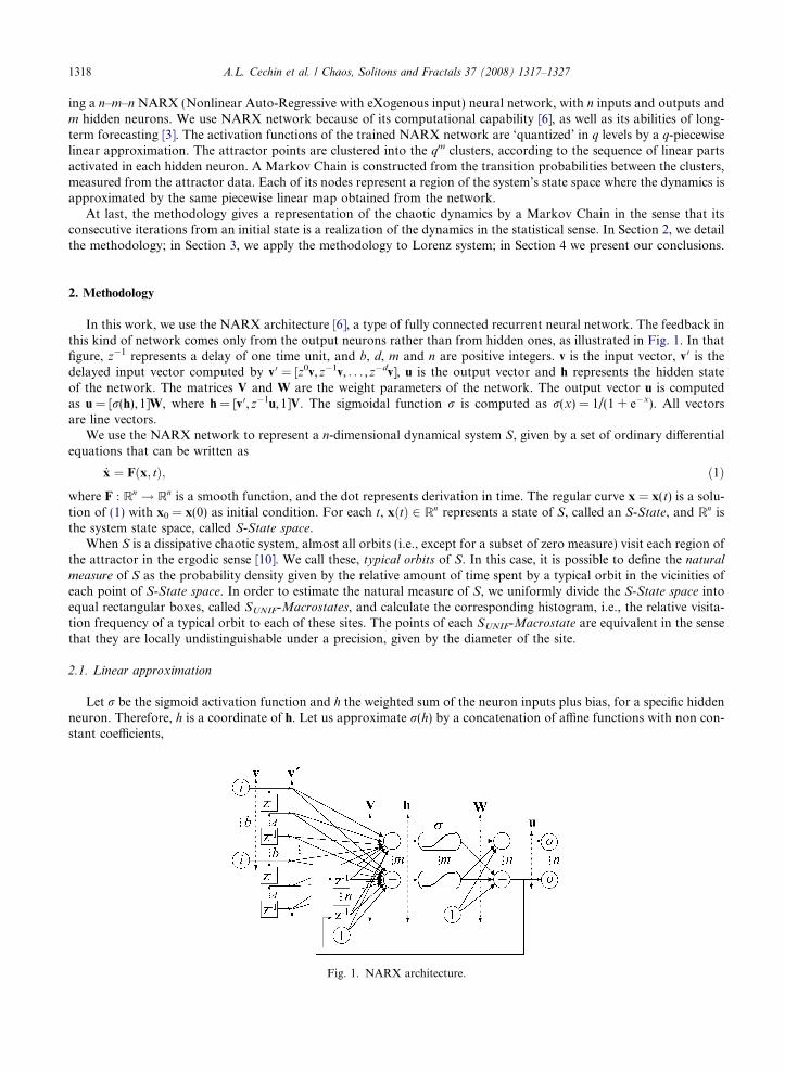
In this work, we use the NARX architecture [6], a type of fully connected recurrent neural network. The feedback inthis kind of network comes only from the output neurons rather than from hidden ones, as illustrated in Fig. 1. In thatfigure, z�1 represents a delay of one time unit, and b, d, m and n are positive integers. v is the input vector, v 0 is thedelayed input vector computed by v 0 = [z0v,z�1v, . . . ,z�dv], u is the output vector and h represents the hidden stateof the network. The matrices V and W are the weight parameters of the network. The output vector u is computedas u = [r(h), 1]W, where h = [v 0,z�1u, 1]V. The sigmoidal function r is computed as r(x) = 1/(1 + e�x). All vectorsare line vectors.

We use the NARX network to represent a n-dimensional dynamical system S, given by a set of ordinary differentialequations that can be written as

_x ¼ Fðx; tÞ; ð1Þ

where F : Rn ! Rn is a smooth function, and the dot represents derivation in time. The regular curve x = x(t) is a solu-tion of (1) with x0 = x(0) as initial condition. For each t, xðtÞ 2 Rn represents a state of S, called an S-State, and Rn isthe system state space, called S-State space.

When S is a dissipative chaotic system, almost all orbits (i.e., except for a subset of zero measure) visit each region ofthe attractor in the ergodic sense [10]. We call these, typical orbits of S. In this case, it is possible to define the natural

measure of S as the probability density given by the relative amount of time spent by a typical orbit in the vicinities ofeach point of S-State space. In order to estimate the natural measure of S, we uniformly divide the S-State space intoequal rectangular boxes, called SUNIF-Macrostates, and calculate the corresponding histogram, i.e., the relative visita-tion frequency of a typical orbit to each of these sites. The points of each SUNIF-Macrostate are equivalent in the sensethat they are locally undistinguishable under a precision, given by the diameter of the site.

2.1. Linear approximation

Let r be the sigmoid activation function and h the weighted sum of the neuron inputs plus bias, for a specific hiddenneuron. Therefore, h is a coordinate of h. Let us approximate r(h) by a concatenation of affine functions with non con-stant coefficients,

Fig. 1. NARX architecture.

A.L. Cechin et al. / Chaos, Solitons and Fractals 37 (2008) 1317–1327 1319

rðhÞ � v0ðhÞL0ðhÞ þ v1ðhÞL1ðhÞ þ v2ðhÞL2ðhÞ; ð2Þ

where L0(h) = 0h + 0, L1(h) = h/4 + 1/2, L2(h) = 0h + 1. v0, v1 and v2 are the characteristic functions of the sets(�1,�2], (�2,2] and (2,+1), respectively. The graphics of r and its approximation are shown in Fig. 2. The threeterms in Eq. (2) represent 1st-order Taylor expansions of r at h = �1, h = 0 and h = +1, respectively.

According to the definitions above, for a NARX network with m hidden neurons, each string s = [s1s2. . .sm], withsi = 0,1,2, indicates which affine component L0, L1 or L2 is activated for each hidden neuron. Each string s is heredenominated NARX-State. Then, each network input u falls in a class defined by the linear components of r. For exam-ple, if m = 5 and [s1s2s3s4s5] = [02112] for a given input, then the NARX approximation is better represented by theaffine components L0(h1), L2(h2), L1(h3), L1(h4) and L2(h5) for the respective hidden neurons. The set of these 3m classesdefines a partition of the S-State. These classes are here denominated SNARX-Macrostates. The NARX-States and theSNARX-Macrostates are then associated in a bijective way.

Let two sigmoid-like functions f(x) and g(x) be approximated, in the uniform sense, like f ðxÞ �P

qvqðxÞ½aqxþ bq�and gðxÞ �

PqvqðxÞ½cqxþ dq�, with

PqvqðxÞ ¼ 1 and vq(x) > 0, where aq, bq, cq and dq are constant coefficients. Then,

the sum f(x) + g(y) may be approximated by

f ðxÞ þ gðyÞ �X

qr

vqðxÞvrðyÞ½aqxþ bq þ cry þ dr�:

In fact,

f ðxÞ þ gðyÞ �X

q

vqðxÞ½aqxþ bq� þX

r

vrðyÞ½cry þ dr� ¼X

q

vqðxÞX

r

vrðyÞ½aqxþ bq� þX

q

vqðxÞX

r

vrðyÞ½cry þ dr�

¼X

q

vqðxÞX

r

vrðyÞ½aqxþ bq þ cry þ dr� ¼X

qr

vqðxÞvrðyÞ½aqxþ bq þ cry þ dr�:

It means that, in order to compute the sum of the output of two hidden neurons, r(hi) + r(hj), it is sufficient to sum thelinear transfer function of each neuron and multiply the corresponding characteristic functions. Also, notice that, be-fore adding the output of the hidden neurons in the output layer, they are multiplied by weights. Again, it is easy toshow that wf(x), where w is the weight between a hidden and an output neuron, may be computed by

wf ðxÞ ¼ wX

q

vqðxÞ½aqxþ bq� ¼X

q

vqðxÞ½waqxþ wbq�:

Therefore, the multiplication by weights does not interfere in the conclusions above. Also, if a constant (bias) c is addedto f(x), an analogous procedure leads to

−6 −4 −2 0 2 4 6

0.0

0.2

0.4

0.6

0.8

1.0

Fig. 2. Function r (dashed line) and its approximation using L0, L1 and L2 (solid line).


cþ f ðxÞ ¼ cþX

q


q

vqðxÞcþX

q


q

vqðxÞ½aqxþ ðbq þ cÞ�:

To put it in a schematic way, the NARX network evaluated at u is approximated by a concatenation of affine appli-cations, which can be matricially represented as

NARXðuÞ �X

s

vsðuÞ ðAsuþ BsÞ; ð3Þ

where the summation is to be performed on all NARX-States, As and Bs are matrices, whose entries result from Eq. (2)together with the affine function operations mentioned above, taking into consideration the structure of the network.

Then, if u(k) is the actual S-State and u(k + 1) the next S-State, corresponding to the network output obtained bythe application of the NARX network on u(k), we can write

uðk þ 1Þ � AsuðkÞ þ Bs; ð4Þ

where s is the NARX-State for which vs(u) = 1.Notice that, there are NARX-States which are not associated to any S-State, and that some of them are associated to

more than one S-State. Inside each SNARX-Macrostate, the S-States are undistinguishable under the composition ofthe affine approximations given by the NARX-State. In opposition to the SUNIF-Macrostates, the SNARX-Macrostates

divide the S-State space in a non uniform way, somewhat respecting the nonuniform characteristics of thedynamics.

2.2. Markov chain representation

Instead of pruning the dynamics by retaining the most visited SUNIF-Macrostates, we do it by keeping the most fre-quently visited NARX-States. This corresponds to a pruning on S-State space to the corresponding SNARX-Macrostates.The advantage of the proposed method is that SNARX-Macrostates define a uniform division, not in the geometric sense,but in the dynamic sense, taking into consideration the linear characteristic of the system. More precisely, each mac-rostate represents a region of good piecewise linear approximation of the system by a specific combination of affinemaps.

In order to prune the 3m SNARX-Macrostates of the n–m–n NARX network, we must adopt some coverage criteria.In this work we retain the SNARX-Macrostates sufficient to cover 95% of the available data. Due to the determinism ofthe chaotic systems, the pruning usually reduce the 3m SNARX-Macrostates to some few relevant for the statisticaldescription of the system.

After the pruning step, a prototype point us in S-State space can be elected to represent each retained SNARX-Mac-

rostate s. These prototypes can be obtained from many methods, depending on the application. For example, for athree-dimensional system, the prototypes can be computed by mean{[u1,u2,u3] : [u1,u2,u3] 2 SNARX-Macrostate}, i.e.,as the mean of the S-States [u1,u2,u3] that belong to the macrostate. The determination of the prototypes is not crucialin the present work, but gives an one-point representation for the SNARX-Macrostates. This contributes to a clearer visu-alization of each SNARX-Macrostate location, which composes the nonuniform geometric partition of the S-State space,as shall be illustrated in Section 3 when we apply the methodology to Lorenz attractor.

Finally, we measure the transition frequency fsr between each pair (s, r) for those most relevant SNARX-Macrostates.These frequencies define the entries of the stochastic matrix of the Markov Chain. Notice that, if s = r, then the tran-sition frequency is associated to the amount of time spent by the typical orbits of the system inside that macrostate.

Using the equation P(s! r) = P(rjs) = P(r \ s)/P(s) and assuming that two different macrostates are independent,the transition probabilities are computed by the following equation

P ðs! rÞ ¼ fsrPr

fsr; ð5Þ

which is the entry (s, r) of the stochastic matrix M defining the Markov Chain for S.Since most dissipative chaotic systems are topologically transitive into their attractors, the stochastic matrix M,

obtained from the aforementioned procedure, is irreducible and aperiodic. Therefore, for a good quality data set,the transitivity properties of the chaotic system S are translated into irreducibility and aperiodicity of M. In this situ-ation, the Stochastic Matrix Theorem says that the sequence of consecutive iterations of M at an arbitrary initial prob-ability distribution p0 tends to a unique stationary probability distribution p1, i.e.,

p1 ¼ limk!þ1

Mkp0: ð6Þ


The stationary distribution p1 of M together with its irreducibility and aperiodicity will be used to evaluate the MarkovChain representation quality.

Let us now summarize the ideas exposed so far. First we list the used nomenclature:

(i) S-State: each point u of the state space of the system.(ii) S-State space: the set of the S-States.

(iii) NARX-State: each string s = [s1s2. . .sm], where si defines which affine approximation, L0, L1 or L2, best representsthe nonlinear activation function r of each of the m hidden neurons, as it is being used to represent the transitionbetween two consecutive S-States.

(iv) SUNIF-Macrostate: each region of a uniform partition of the S-State space into equal boxes.(v) SNARX-Macrostate: the set of the S-States associated to a specific NARX-State s.

(vi) M: the stochastic matrix of the Markov Chain, whose entries are the transition probabilities between the retainedNARX-States.

The steps to obtain the Markov Chain are the following:

(i) Attractor reconstruction from the data set by the use of Takens–Mane technique [7,9].(ii) Training of a n–m–n NARX network with the reconstructed attractor.

(iii) Determination of NARX-States, based on the proposed linear quantization for the activation function r.(iv) Pruning of the set of NARX-States, retaining only the most relevant ones.(v) Determination of the SNARX-Macrostates associated to each of the retained NARX-States.

(vi) Determination of prototypes for each retained SNARX-Macrostate.(vii) Calculation of the stochastic matrix of the Markov Chain, whose entries are given by the probability of transition

between the pairs of the retained NARX-States.(viii) Verification of Stochastic Matrix Theorem for M to test the overall quality of the analysis.

3. Application to the Lorenz equations

The methodology was applied to chaotic data obtained from numerical integration of Lorenz System. These equa-tions were proposed by Edward Lorenz in 1963 as a simplified model for wheather forecast, describing the motion of afluid in a horizontal layer being heated from below. Lorenz equations are

_x ¼ aðy � xÞ ð7Þ_y ¼ rx� y � xz ð8Þ_z ¼ xy � bz ð9Þ

where x = x(t), y = y(t), z = z(t) are the unknowns, a, r and b are parameters and the dots denote derivation in time.Working on the numerical solutions of his equations for a = 10, r = 28 and b = 8/3, Lorenz found, for the first time,

computational evidences of dissipative chaotic dynamics. In fact, for that set up of parameters, Lorenz system exhibitschaotic behavior with a strange attractor, illustrated in Fig. 3.

We integrated Lorenz equations with a four order Runge–Kutta method from an initial condition inside the attrac-tor, and obtained a data set {[x(k),y(k),z(k)] :1 6 k 6 N}, of N = 10,000 points. These points are Dt = 0.01 apart fromeach other. In order to simulate a usual situation where only one time series is available, we only used the x(k) timeseries. This is like if we had just one sensor, allowing the acquisition of only one observable.

It can be seen that each wing of the attractor is almost perfectly planar, which is in accordance with its fractal dimen-sion next to two. Each wing is centered at an unstable stationary point around which the typical orbits circulate. Begin-ning on the right wing, the pathway runs counter clockwise with an increasing radius. When a critical radius is reached,the orbit eventually migrates to the other wing to behave in the same way. Therefore, the global behavior of the typicalorbits of the system is composed by two kinds of movements: circulation around the unstable centers of the wings andmigrations from one wing to the other.

3.1. Network training

The time lag Dt = 0.01 is already suitable for the Lorenz attractor rebuilding, according to the criteria of autocor-relation function zero crossing [1]. Therefore, we applied Takens–Mane embedding technique, considering the three

–20

–10

0

10

20

–30–20

–100

1020

30

0

10

20

30

40

50

yx

z

Fig. 3. Lorenz attractor with a = 10, r = 28 and b = 8/3.

Fig. 4. Projections of Lorenz attractor obtained from the original time series (left panels) and from the trained NARX network (rightpanels) on two of the principal components: u1 · u2 (upper panels) and u1 · u3 (lower panels).



dimensional vector time series X = {[x(k),x(k � 1),x(k�2)];3 6 k 6 N}. Then, we applied principal component analysison X to obtain centered decorrelated data. The data were normalized to have zero mean and standard deviation equalto one. We finally arrived at a centered and normalized set of three dimensional vectors U = {u(k) =[u1(k),u2(k),u3(k)]; 3 6 k 6 N} with decorrelated coordinates. This improves the network training because of the inde-pendence between the principal components. The left panels of Fig. 4 show projections of Lorenz attractor on the prin-cipal components u1 · u2 and u1 · u3.

We trained a 3-m-3 NARX network (see Fig. 5) with the data set U = {u(k);3 6 k 6 N}. We used a NARX networkwith one hidden layer, since it can represent any nonlinear function [4,5]. The output neurons use linear activation func-tions, which does not impair the capacity of the network to represent nonlinear maps. Short-cut connections were usedin all tried network structures. The short-cut connections implement the linear mapping from inputs to outputs, whilethe connections through the hidden neurons implement the nonlinear mapping.

Under those circumstances, a 3–5–3 NARX network with a sigmoid activation function was shown to be able tolearn the essential of Lorenz dynamics. For each initialization, the network was trained 5000 epochs with the BFGS(Broyden-Fletcher-Goldfarb-Shanno) algorithm, and the network with the smallest square error was chosen.

Fig. 5. Structure of the 3-m-3 NARX network with m = 5. This structure implements u(k + 1) = NARX(u(k)) as an approximation forLorenz dynamics.

1 7 14 22 30 38 46 54 62 70 78 86 94

020

040

060

080

010

0012

00

1 7 14 22 30 38 46 54 62 70 78 86 94

020

040

060

080

010

0012

00

Fig. 6. Histogram of Lorenz attractor obtained from U (left), and by iterating the trained NARX network.


The smallest attained sum of square errors was 0.029 corresponding, in average, to 0.098% of the standard deviationof each output. Moreover, the orbits generated by the used network presented very similar statistical patterns whencompared with Lorenz system, in the sense that the natural measures of the system and of the network are similar.In order to verify this property, due to the quasi-planar geometry of the attractor, it was enough to consider the pro-jection of the set U on the plane u1 · u2 (see Fig. 4). We divided the relevant rectangle [�2.5,2.5] · [�3.0,3.0] into 100rectangular SUNIF-Macrostates, each one labeled with a number from 1 to 100. Then, the histograms were computed forU and for a typical orbit of NARX network, inside its attractor. The typical results are illustrated in Fig. 6, which showsthe similarities. The p-value is 0.9996 for KS (Kolmogorov-Smirnov) test, attesting a high statistical similarity betweenboth histograms.

3.2. Extraction of markov chain

Applying the algorithm to the best network resulted in 35 NARX-States. For pruning the 35 NARX-States, weadopted the criteria of 95% coverage of the data in the training data set. The pruning reduced the model to the 13 mostrelevant NARX-States, covering 95.6% of the data (See Fig. 7). The most occupied NARX-State has 32.70% of the dataand is defined by the string s = [11111].

The prototypes us, computed as mean{u:u 2 SNARX-Macrostate associated to the s NARX-State} are listed in Table 1in a decreasing order of relevance. It is shown their corresponding NARX-States, their number of data points, and theircoordinates. The prototypes locations are illustrated in Fig. 8. From that figure and Table 1 we can see that the mostoccupied states are those next to the center of the attractor. This can be partially explained based on the low velocity ofthe orbits next to the origin.

By the use of Eq. (5), we obtained the transition probabilities of the Markov Chain stochastic matrix, from the num-ber of transitions between the NARX-States (Fig. 9). The obtained Markovian model M is shown in Fig. 10, wherearrows represent the direction of transitions with their probabilities indicated at their respective right sides. For exam-ple, the probability of a typical orbit going from NARX-State 1 to NARX-State 4 is P(1! 4) = 0.362% � 0.4%,obtained as 12

3197þ17þ12þ38þ5þ43, according to the last line of transition frequency matrix shown in Fig. 9.

The Markov Chain associated to M gives a statistical description of Lorenz dynamics in the attractor. For example,consider a S-State in SNARX-Macrostate 4. Then, according to M, there is 93.5% of chance that the corresponding orbitwill remain in this same SNARX-Macrostate and, therefore, the mean time a S-State stays in 4 is approximately given bylogð0:5Þ

logð0:935Þ ¼ 10:36 iterations. Analogously, once in SNARX-Macrostate 1, the orbit stays there for 19.6 iterations and then

1 2 3 4 5 6 7 8 9 10 11 12 13 14 15 16 17 18 19 20 21 22 23 24 25 26 27

0.00

0.05

0.10

0.15

0.20

0.25

0.30

Fig. 7. Histogram of occupation by the points of U. Only the 27 most relevant SNARX-Macrostates are shown. From these, it wasretained the 13 most relevant (in gray), covering 95.6% of the data.

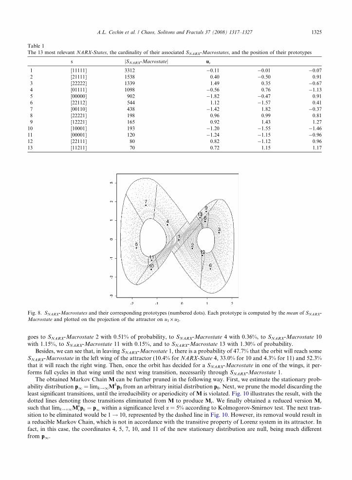
Table 1The 13 most relevant NARX-States, the cardinality of their associated SNARX-Macrostates, and the position of their prototypes

s jSNARX-Macrostatej us

1 [11111] 3312 �0.11 �0.01 �0.072 [21111] 1538 0.40 �0.50 0.913 [22222] 1339 1.49 0.35 �0.674 [01111] 1098 �0.56 0.76 �1.135 [00000] 902 �1.82 �0.47 0.916 [22112] 544 1.12 �1.57 0.417 [00110] 438 �1.42 1.82 �0.378 [22221] 198 0.96 0.99 0.819 [12221] 165 0.92 1.43 1.27

10 [10001] 193 �1.20 �1.55 �1.4611 [00001] 120 �1.24 �1.15 �0.9612 [22111] 80 0.82 �1.12 0.9613 [11211] 70 0.72 1.15 1.17

Fig. 8. SNARX-Macrostates and their corresponding prototypes (numbered dots). Each prototype is computed by the mean of SNARX-

Macrostate and plotted on the projection of the attractor on u1 · u2.


goes to SNARX-Macrostate 2 with 0.51% of probability, to SNARX-Macrostate 4 with 0.36%, to SNARX-Macrostate 10with 1.15%, to SNARX-Macrostate 11 with 0.15%, and to SNARX-Macrostate 13 with 1.30% of probability.

Besides, we can see that, in leaving SNARX-Macrostate 1, there is a probability of 47.7% that the orbit will reach someSNARX-Macrostate in the left wing of the attractor (10.4% for NARX-State 4, 33.0% for 10 and 4.3% for 11) and 52.3%that it will reach the right wing. Then, once the orbit has decided for a SNARX-Macrostate in one of the wings, it per-forms full cycles in that wing until the next wing transition, necessarily through SNARX-Macrostate 1.

The obtained Markov Chain M can be further pruned in the following way. First, we estimate the stationary prob-ability distribution p1 = limk!1Mkp0 from an arbitrary initial distribution p0. Next, we prune the model discarding theleast significant transitions, until the irreducibility or aperiodicity of M is violated. Fig. 10 illustrates the result, with thedotted lines denoting those transitions eliminated from M to produce Mr. We finally obtained a reduced version Mr

such that limk!þ1Mkr p0 ¼ p1 within a significance level a = 5% according to Kolmogorov-Smirnov test. The next tran-

sition to be eliminated would be 1! 10, represented by the dashed line in Fig. 10. However, its removal would result ina reducible Markov Chain, which is not in accordance with the transitive property of Lorenz system in its attractor. Infact, in this case, the coordinates 4, 5, 7, 10, and 11 of the new stationary distribution are null, being much differentfrom p1.

r

s

1 2 3 4 5 6 7 8 9 10 11 12 13

12

34

56

78

910

1112

13

3197 17 12 38 5 43

59 1446 21 11

1264 75

56 1027 15

844 58

28 469 47

59 379

51 147

24 16 125

24 155 14

34 86

47 11 22

3 40 27

Fig. 9. Transition frequencies between pairs of NARX-States. The entries (s, r) are fsr, the number of transitions from the NARX-State

s to the NARX-State r. Black boxes represent more probable transitions.

1 96.5

2

0.5

4

0.4

10

1.1

11

0.2 13

1.33.8

94.1

8

1.412

0.7

3 94.4

6

5.6

5.1

93.5

1.4

5 93.6

7

6.4

5.1

86.2

8.6

13.5

86.5

25.8

74.2

9

14.5

9.7

75.812.4

80.3

7.3

28.3

71.7

58.8

13.8

27.5 4.3

57.1

38.6

Fig. 10. Markov Chain M obtained with our methodology and its reduced version Mr for a = 5%. The dotted transitions are thoseeliminated from M to define Mr. The dashed transition 1! 10 would be the next one to be eliminated, but violating the ergodicity ofthe Markov Chain.


4. Conclusion

In this paper, we propose a methodology for statistical modeling a chaotic system from one observable (time series).The method is based on the reduction of a trained NARX network to a Markov Chain where each of its states is aregion of good piecewise linear approximation, given by a specific combination of the functions L0, L1 and L2, as givenby Eq. (2). The found Markov Chain represents the chaotic attractor in its statistical essence, loosing only the least sig-nificant (i.e., less probable) movements. We illustrate the methodology applying it to Lorenz system.


An obvious way to arrive in a Markov Chain would be to follow the original ideas of Ulam [11], and divide therelevant region of the state space (the smallest parallelepiped containing the attractor) uniformly into cubic regions,the SUNIF -Macrostates. Then, we would discard those SUNIF-Macrostates in which the typical orbits spend the leastamounts of time. After that, we could also construct a Markov Chain with its nodes representing each one of theretained macrostates, and the probability transitions given by the data set. This Markov Chain would also approximatestatistically the chaotic system S in its transitions from a SUNIF-Macrostate to another.

However, the manifestation of the nonlinear effects of a chaotic system is not homogeneous in the state space. In thecontrary, there are regions where the system behaves more as a linear system and others where nonlinearity effects arepredominant. Therefore, an important drawback of the homogeneous approach above is to consider a uniform divisionof state space, in which the macrostates have the same relevance in the dynamics. This would lead us far from an opti-mized representation, resulting in a much more complex Markov Chain with a much larger number of macrostateswhen compared to our technique. Our methodology takes inhomogeneous characteristics of nonlinearity of the systeminto consideration.

In the paper, we focused our discussions on a three-level quantization, i.e., using only three affine functions L0, L1

and L2 to approximate the activation function. However, a more refined quantization L0,L1, . . .,Lq�1 could be applied.Generally speaking, as q grows, the diameter of each SNARX -Macrostate tends to get smaller, while the number ofSNARX-Macrostates tends to grow, as well as the accuracy of the piecewise linear approximations. In the limit, the modeltends to a Markov Chain with a number of states equal to the points of the reconstructed attractor, and a stochasticmatrix composed of rows of zeros and a unique entry equal to one. In other words, the Markov representation tends toa deterministic finite-state machine. The establishment of a precise criterion for the degree of quantization depends onthe application. Although, the general idea is that higher degrees of quantization are necessary for more intensenonlinearities.

The Markov Chain obtained using the proposed methodology is, in fact, a first order Markovian model for the sys-tem, and presents an important imperfection. Indeed, some transitions, possible for the 1st order Markov approxima-tion, may never occur in the real system S. For example, while the transition 1! 4! 1 is impossible for a Lorenzsystem orbit, there is a chance for that transition to occur, according to the obtained Markovian Chain. In order toeliminate such 1st order artifacts, we should go one step ahead and obtain a 2nd order Markov Chain for the system,whose states would be the transitions between two of the states of the Markov Chain obtained so far. Once again, 2ndorder artifacts will remain, demanding a step ahead in the modelling. At the end, one would obtain a kth-order Mar-kovian Model constituted of a set of Markov Chains without ith order artifacts, for i 6 k. The details of these higherorder Markovian Models are left for a future work.

References

[1] Abarbanel HDI. Analysis of observed chaotic data. San Diego: Springer; 1996.[2] Cannas B, Cincotti S. Neural reconstruction of Lorenz attractors by an observable. Chaos, Solitons & Fractals 2002;14:81–6.[3] Lin T, Horne BG, Tino P, Giles CL. Learning long-term dependencies in NARX recurrent neural networks. IEEE Transact

Neural Network 1996;1(6).[4] Hornik K, Stinchcombe M, White H. Multilayer feedforward networks are universal approximators. Neural Networks

1989;2(5):359–66.[5] Hornik K. Approximation capabilities of multilayer feedforward neural networks. Neural Networks 1991;4(2):251–7.[6] Siegelmann HT, Horne BG, Giles CL. Computational capabilities of recurrent NARX neural networks. IEEE Transact Syst, Man

Cyb – Part B: Cyb 1997;27(2):208–15.[7] Takens F. In: Detecting strange attractors in turbulence. Lecture notes in math, vol. 898. Springer Verlag; 1981.[8] Tronci S, Giona M, Baratti R. Reconstruction of chaotic time series by neural models: a case study. Neurocomputing

2003;55:581–91.[9] Mane R. On the dimension of certain compact invariant sets of nonlinear maps. Lecture Notes in Math 1981;898.

[10] Pollicott M. Lectures on ergodic theory and Pesin theory on compact manifolds. London mathematical society lecture note series,vol. 180. Cambridge University Press; 1993.

[11] Ulam SM. Problems in modern mathematics. Interscience; 1964.

optimizing markovian modeling of chaotic systems with recurrent neural networks

Documents