OPTIMIZING BINARY TREES GROWN

WITH A SORTING ALGORITHM

W. A. MARTIN — D. N. NESS

421-69

MASSACHUSETTS[NSTITUTE OF TECHNOLOGY

-0 MEMORIAL DRIVE

BRIDGE, MASSACHUSETTS

OPTIMIZING BINARY TREES GROWN

WITH A SORTING ALGORITHM

W. A. MARTIN — D. N. NESS

421-69

[^l:wcY libraryJ

H02i

Hi.

OPTIMIZING BINARY TREES GROWN WITH A SORTING ALGORITHM

W. A. MARTIN — D. N. NESS

Tree Growing Processes

In this paper we consider a process which grows and uses a labeled

binary tree structure. Each node in this structure has an item of

information, an upward pointer, and a downward pointer. The upward

and downward pointers may point to null elements.

At any node in the strcuture all items of information in the ''tree rijh^i''^ '^*^J*^

which are larger* than the item of information at that node will be in

the subtree pointed to by the upward pointer. Similarly, all smaller

items are in the sub-tree pointed to by the downward pointer. In this

paper we will not consider contexts where multiple nodes have the same

item value.

Such trees are easy to grow. The first element is placed at the

root. Thereafter each new element is placed in the tree by comparing

it with the root and moving up or down depending on whether the new

element is larger or smaller. This process is repeated at each node

until an attempt is made to move to a null node. The item is then placed

at this point in the tree. (We call this algorithm "A" below.)

Obviously the measure can be any kind of computation.

As an example, consider adding the item 40 to the tree:

Figure 1

The following steps will be performed:

1) 40 > 10 ^ move up

2) 40 < 60 -> move down

3) 40 > 30 ^ move up

4) 40 < 50 -^ move down

Since there is no item down from 50, 40 is attached at this point. This

algorithm can be used for building symbol tables and it Is closely related

to the sorting algorithm, QUICKSORT (3,4).

Let us now consider some mathematical properties of the tree struc-

tures that are grown by this algorithm.

Mathematical Characteristics

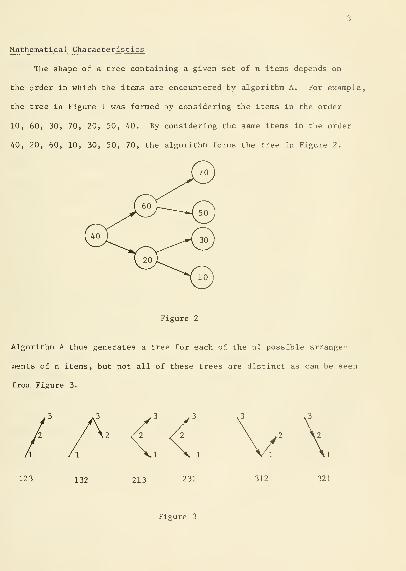
The shape of a tree containing a given set of n items depends on

the order in which the items are encountered by algorithm A. For example,

the tree in Figure 1 was formed by considering the items in the order

10, 60, 30, 70, 20, 50, AO. By considering the same items in the order

40, 20, 60, 10, 30, 50, 70, the algorithm forms the tree in Figure 2.

Figure 2

Algorithm A thus generates a tree for each of the n! possible arrange-

ments of n items, but not all of these trees are distinct as can be seen

from Figure 3.

132 213

Figure 3

In the analysis to follow we will consider each of the nl permuta-

tions of the n items to be equally probable. Thus, some trees will be

generated more often than others. We will also mention the results which

obtain for the case where each distinct tree is taken as equally probable.

We can search for an item in a tree by following exactly the same

steps used to insert the item while the tree is being constructed. It seems

reasonable to assume that the time required is proportional to the number

of nodes visited. (For example, see Figure 6) It is easy to see that

one can find each of the items in the tree in Figure 2 by visiting a

total of 17 (= 1*1 + 2*2 + 4*3) nodes, while one must visit 22 (= 1*1 +

1*2 + 2*3 + 2*4 + 1*5) nodes to find the same items in the tree in Figure 1.

*Clearly, the tree in Figure 2 is not only better, but optimum. We have

devised an algorithm (Algorithm B) ,presented belov7, which will convert

any tree generated by Algorithm A into an optimum tree containing the

same items. Algorithm B requires a time proportional to the number of

items (see Figure 7). It is natural to ask whether the time thus saved

in searching a reorganized tree is greater than the time required for the

conversion from the non-optimal into the optimal form.

To this end, let us calculate the number V(n) of nodes visited per

item, in finding each item in each of the n! trees containing n nodes.

Let V(n) be the number of nodes visited in finding each item in each of

See Reference (5), page 402.

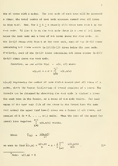
the n! trees with n nodes. The root node of each tree will be accessed

n times; the total number of root node accesses summed over all trees

is thus n-n!. Now, for 1 £ k £ n exactly n!/n trees have item k at the

root node. If item k is at the root node there is a tree of k-1 items

below the root node and a tree of n-k items above the root node. In

the (n-1)! trees with item k at the root node, each of the (k-1)! trees

containing k-1 items occurs (n-1) ! / (k-1) ! times below the root node.

Similarly, each of the (n-k)! trees containing n-k items occurs (n-1)!/

(n-k)! times above the root node.

Therefore, we can write V(n) = u(n, n!) where

n-1u(n,m) = n-m + 2^^ u(k,m/n)

k=0

u(n,m) represents the number of node visits summed over all trees of n

nodes, where the forest (collection of trees) consists of m trees. The

formula can be obtained by observing the root node is visited n times

for each tree in the forest, or a total of n-m node visits. For each

value of the root node (1/n of the trees in the forest have the same

root nodes) the upper (and lower) trees are a forest of m/n trees, and

consist of k (k = 0, . . ., n-1) nodes. Thus the rest of the upper (or

T \ ^ . n-1lower) tree requires v ^i / \

I u(k,m/n) visits.k=0

Since V(n) = ^^^^^n I

^ .. ^- J ~/ \ u(n,m),

2 y u(k,m/n )we want to find u(n,m) = = n H > -.

m n1 n ^'^

Note: u(0,m) =

So we can see by induction that u is not a function of m and we can

2""^ -

write Vlh)= n + -I V(k).

'^ k=0

From this we findV(n) = -^ii V(n-l) + 2 - -

n n

3)

4)

andn+1

V(n) = - n + 2 (n+1) I ji=2

5)^

The sum in 5) can be bounded by the log function to give the bounds.

V(n) < - n + 2 (n+1) log n 6)

n+1

Thus, for large n we have V(n) - 2nlogn. 8)

This result has been obtained by Hibbard (3).

Now, for comparison, we derive an expression for the number r(n) of

node visits for an optimum tree of n items. If 2-1 £ n < 2 -1 we have

r(n) =/j2^ - 2^ + lN+ (j + 1) (n - 2^ + 1)

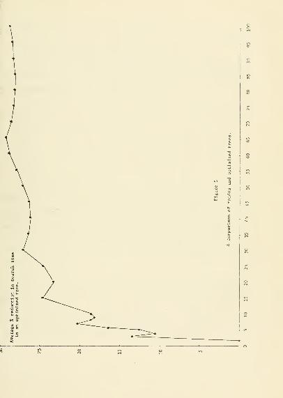
In order to compare the average trees with the optimum, the function

(n) - r(n) ^^ plotted in Figure 5. For the plotted values the optimum

tree gives an improvement of 10 to 30%. To examine this improvement

Note: V(l) =

z.--=

X- /

x^^'-i

further note that for large n and for n=2 -1 , r(n) approaches —;—°—- .

log2

The improvement is then ~ .386 nlog n (.386 = 2 log 2-1).

Since the time it takes our Algorithm B to form an optimum tree is

proportional to n, there is some n beyond which application of the algo-

rithm must result (on the average) in a saving.

Referring to Knuth (5) we may also note that if we take all distinct

labeled trees to be equally probable we obtain the result V(n) - xCsfn

for large n. This would make application of our algorithm even more

profitable on the average. It suggests that those distinct labeled

trees which are generated more than once by Algorithm A are often the

"good" ones.

The above calculation suggests exactly how inefficient we can expect

the "average" tree to be. It must be recognized, however, that the actual

tree grown in any given case may depart even more substantially from the

optimum. If the data were to be incorporated in ascending sequence, for

example, each item would be placed "up" from all previous items, and our

process would reduce to linear search with a time to access all items

2proportional to n .

It is obviously easy to extend the algorithm presented above to

allow us to maintain information about the efficiency of the structure

as it is being grown. If we start a counter at 1 and then increment it

each time a comparison is performed in the process of placing that element

in the tree, we obtain a count of the number of comparisons necessary to

find this element. If we accumulate this number as we bring in each new

item we will always have the number of node visits to access all items available.

This information may suggest, then, that at some point it would be

worth restructuring a tree as it is being grown or after it has been

grown but before some searches are to be performed. We now present our

algorithm for performing this restructuring.

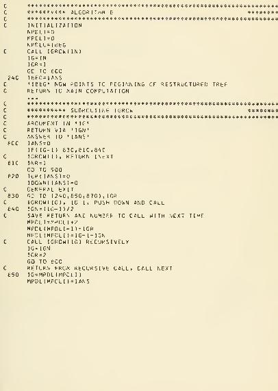
The Restructuring Algorithm (Algorithm B )

The algorithm is presented here in English; it is also presented

in the Appendix in FORTRAN.

The procedure IBEST returns as its answer a pointer to the root

node of the restructured tree. This procedure also establishes the envi-

ronment for the other subroutines: IGROW and NEXT. IBEST computes IGROW(n),

where n is the number of nodes in the tree to be restructured. It returns

the result of this comoutation (which is the restructured tree) as its answer.

The procedure IGROW (n) is responsible for constructing an optimum

tree containing n nodes. It must be recursive as it may call itself. It

uses the procedure NEXT, which returns a pointer to the smallest node in

the old tree the first time it is called and a pointer to the smallest node

not previously returned on each successive call. IGROW (n) can take three

courses of action:

1) If n = , return a pointer to a null node.

2) If n = 1 , call NEXT and return its result.

10

3) If n > 1

a) Call IGROW (L(n-1)/2J)

b) Call NEXT

c) Call IGROW ([(n-l)/2l)

Then alter the node pointed to by the result of b) by replacing its

up pointer with the result of a) and its down pointer with the

result of c) . Return the result of b) , thus altered, as the answer.

The procedure NEXT moves through the original tree structure returning

the nodes in ascending sequence. Given a tree, it returns the nodes in the

lower branch by calling itself recursively with this branch as argument,

then it returns the root node, and then the nodes in the upper branch. It

is convenient to think of NEXT and IGROW as coroutines. It should be noted

that IGROW does not need to modify the pointers of any node until NEXT is

completely through with it. Thus the nodes of the original tree can be

patched directly and no additional memory is required.

Incremental Restructuring

If one wishes to form an optimum tree each time a new node is added,

then it is not necessary to use a global restructuring method like Algo-

rith B. A method which concentrates on those nodes visited during the

addition of the new node can be used. We are not aware of such a method

which is highly efficient. However, a good method is known for main-

taining a tree structure which may not be optimum, but is very good (1,2).

11

This tree structure is characterized by the constraint that the

maximum path length of the subtree above a given node cannot differ by

more than one from the maximum path length of the subtree below that

node. This constraint excludes the really bad trees formed by algorithm

A and so the average number of nodes visited per item searched must be

less than 21ogn, but slightly more than for an optimum binary tree. This

has been verified numerically by Foster (2). Such a tree is shown in

Figure 4.

In order to make the method of adding a new node efficient, each

node must have associated with it a number indicating the amount by

which the maximum path length of the upper subtree exceeds the maximum

path length of the lower subtree. In Figure 4 these numbers are shown

in brackets next to each node. A new node is added to this struc-

ture in two steps. First, the node is added to the tree using algorithm

A. However, a pointer to each node visited should be placed on a push-down-

list so that the path can later be retraced to restructure the tree. (Note that

12

the tree cannot be altered to meet the path length constraint until

the new node is in place, because the maximum path length of a sub-

tree containing the new node depends on exactly where the new node

is added.) The tree is then restructured by applying algo-

rithm C. To apply this algorithm one traces back along the path

followed in adding the new node. At each node along this path one

of the following conditions will hold:

a. Either the upper or lower subtree was previously longer by

one and now they are the same length. In this case no re-

structuring is needed and it is not necessary to move back

toward the root node any farther since the length of the

subtree extending from this node is unchanged.

b. Both subtrees were previously the same length and now one

of them is longer by one. No restructuring is done but the

path must be retraced farther, since the length of the sub-

tree extending from this node has increased by one.

c. A subtree which was previously longer by one is now longer

by two. The tree must be restructured at this node but the

path need not be retraced any farther since the restructuring

will return the subtree to its original length.

In order to explain the restructuring algorithm let us assume that

the lower subtree is longer, so that the tree has the form:

(m)

(m+2))

y

13

A and B are subtrees of length m and m+2 respectively. To

restructure we save a pointer to node p and examine subtree B.

It will either have the form:

I)-C (m)

(m+1)

or the form:

II)

C (m+1

(m)

5

since it was of length m+1 before the new node was added, and the new

node increased its length without unbalancing it so that it needed

to be restructured.

In case I) the restructuring is completed by forming the tree:

14

In case II) we examine subtree C. If m ^ it will have one of the

forms:

III)

IV) For m = subtree C will just be a single node.

In case III) the restructuring is completed by forming the tree:

Finally, in case IV) the final tree has the form:

One can now verify that each of these restructuring operations

returns the subtree to its length before the new node was added.

Furthermore, it is easy to see that the effort required to restructure

once a node with unbalanced subtrees has been located is independent

of the size of the entire tree.

15

No one has given an exact analysis of the effort required to

add a new node to the tree and then retrace the path until a node

in either condition a) or c) is found. Foster (2) argues that for

large trees the average effort to retrace and the fractional number

of times each case of restructuring is applied are independent of

the size of the tree. If this is the case then the total average

effort to apply algorithm C while building a large tree is propor-

tioned to n, the number of nodes, just as it is for algorithm B.

A Comparison of the Global and Incremental Restructuring Algorithms

We can then propose two strategies for building a tree of n items.

a. Apply algorithm A n times and then apply algorithm B once.

b. Apply algorithm A n times and apply algorithm C each time

algorithm A is used.

Strategy a) will require an effort A nlog n + Bn, for some con-

stants A and B. Strategy b) will require, under the assumptions of

Foster, effort A.nlog n + Cn. Strategy b) keeps the tree organized

at each step and this would tend to make A„ less than A^ . On the other

hand, strategy b) requires saving pointers to the nodes visited on a

push-down-list and this would tend to make A„ greater than A^ . Strategy

a) always leaves us with an optimum tree while strategy b) leaves us with

a tree which is slightly less than optimum. In addition, strategy b)

requires slightly more storage.

16

Experimental Results

Programs for strategy a) and strategy b) were coded in FORTRAN

for the IBM 1130. Algorithm C is longer and more difficult to pro-

gram than algorithm B. Figure 6 shows the average compution time/

node visited as a function of the size of the tree being searched by

algorithm A. Trees of a given size were generated at random; the

same results also held for worst trees.

Figure 7 shows the average computation time/item for application

of algorithm B to random trees of different sizes.

Figure 8 shows the average time/item to apply strategy a) and

strategy b) as a function of the size of the tree. The solid line is

fitted to the points for strategy a) and the broken line is fitted to

the points for strategy b). It can be seen that strategy b) is slightly

faster for trees of less than 1000 items.

Conclusions

Trees grown without any reorganization are quite good on the average.

Reorganization is a second order improvement, and so a decision to use

algorithm B or algorithm C depends on how the information is to be

accessed.

17

O >-l 4-1

cr 4-j 01 ex

18

6 C w

•u x: ^

D <4-i x:cr c ij

^^ Q 3

c

2AC

*******«««««INITIANPCL 1=

KPCL 1 =

\PrLU=CALL I

IG= IN

IGR = 1

GC TOletG-I•IBEG*RETURN

****t***«*****«*«*«**«=t*«**«****«««****«*««****««««*«««*i***>!** ALGORITHM E *««**«««**#«*«*««««««* V***«*«*4*«*«*«*«*«««*«*«««*****«««*«*iC.«*LIZAflON

IBEGGRCtsdN)

8CCANSNOW POINTS TC PEGINNING CF RESTRUCTURED TREETO MAIN CONPLTATION

ecc

eic

820

830

EAG

fc50

ARGUNENRETUKNANSVvERIANS=0IF( IG-lIGRCW( I

INR=lCO TO 9

ILP( IANIDOVnNJ I

GENERALno TO {

IGROWt I

IGN=( IGSAVE HEMPCL I = ^'

MPHL (MPMPDL (MPCALL IG

IG=IGNIGR = 2

GO TO e

RETLRNIG^MPDLMPDL (MP

««**««*«*«**«****««*««*»***«*««*««***«*****»**** SLBRCLTINE IGRCU«*«*«*««*<:*«#«*««««*«*«*«*«*«*«***«**««****«****T IN • IG'

VIA MGN'TO • lANS'

) fc3C,eiC,8AC), RETURN INEXT

00S) =

ANS)=0EXIT

2^0,850,870), IGRG), IG 1, PUSH DOWN AMD CALL-1 )/2TURN AND NUMBER TO CALL WITH NEXT TIMEPDLI+2DLI-n-IGROLl )=IG-I-IGNROW{ IG) Recursively

ccFRCM RECURSIVE CALL, CALL NEXT(MPCLI

)

CLI ) = IANS

no TO 9C0C RETURN FROM MEXI, CALL IGRCVs RECLRSIVELY AGAIN860 MPCL I=MFCL I+l

^PCL (NPCLI )=IANSIGR = 3

GC TC 8CCC RESTRLCTLKt AS IS APPRCFRIATE870 IG = NPrL {NPCLI )

ILP( IG)=IANSIDGWN( IG )=MPCL(MP0LI-1)IANS=IG

C POP THE STACK ANC RETLRNIGR = NPDL(MPDLI-2)MPOL I = MPCLI-3GO TO 820

C *«««««**«« SUBROUTINE NEXT *C NPCLU CONTAIKS NCDE TO REGIN COWNV^ARD PATH, UNLESS iERO900 IF(NPDLU) 910,S2C,SIC

C PUSH CURRENT NCCE AND CHAIN CCUNt^ARDS910 NPDLl=NPCLI+l

NPDLCNPDLI )=NPDLUNPCLU=IDOkvN(NPDLU)GO TO 9CC

C NC FURTHER CHAIN, RETURN A VALUE AND POP STACK920 IANS=NPDL(NPDLI )

NPDLI=NPDLI-1NPCLU=IUF{ lANS)

C EXITGO TO (820,860), INREND

23

REFERENCES

1. Adel 'son-Vel'skiy , G. M. , and Landis, Ye. M. , "An Algorithm forthe Organization of Information," Deklady Akademii Nauk USSR ,

Moscow, p. 263-266; Vol. 16, No. 2, 1962; also available in

translation as U.S. Dept. of Commerce OTS, JPRS 17,137, Washing-ton, D.C., and as NASA Document N63-11777.

2. Foster, C. C. , "Information Storage and Retrieval Using AVL Trees,Proc. ACM 20th National Conference , (1965), p. 192-205.

3. Hibbard, T. N. , "Some Combinatorial Properties of Certain TreesWith Applications to Searching and Sorting," JACM 6 (May 1963),206-213.

A. Hoare, C. A. R. , "Algorithms 63, Partition, and 64, Quicksort,"CACM 4 (July 1961), p. 321.

5. Knuth, D. E. , The Art of Computer Programming , Vol. 1, Addison-Wesley, (1968), Section 2.3.4.5.

c^'

Mmj^

Date Due

OEC 05 75

.a#I^R

UPr 44 7<

»R2 8

JUN Id '90,

07 199Z-

APR. i 3 7534

MOV. < 3«XF

«»R 3 78.8<J

^nm

?P^PFCl8l98q

Fga

—

sr'n

9!?'

3 TDflO DD3 7D2 171

3 ^QflD DQ3 7D2 153

i/ZP'^f

iiiiiiiiiHi'i'iiiiiiiiiyiiiiiiiiiiij''^''^

3 IDflD DQ3 1,71 115

iiiiii'irriijiiie3 lOaO 003 705 150

''^'

Illlllir'l11'"'l!l'''f'''lf'l'11'f''''l ' '-ri

3 1060 DD3 b71 16^

^21 '^'f

3 lOaO 003 b71 1B7

3 1060 003 b71 17b

^r^'fc^

3 lOflO 003 b71 Ibfl

"/^y-^f

3 lOflO 003 705 5b0

3 1060 DQ3 705 555

iiiiiilliiili-'-"

3 1Q60 003 705 545