optimization of the geometry of communication for autonomous missions of underwater ... ·...
TRANSCRIPT

UNIVERSITÀ DI PISA
1 343
INS
UP
R
EMÆ DIG
NIT
AT
IS
Universita degli Studi di Pisa
DIPARTIMENTO DI INGEGNERIA DELL’INFORMAZIONE
Corso di Laurea Magistrale in Ingegneria Robotica e dell’Automazione
Tesi di Laurea Magistrale
Optimization of the Geometry of Communication forAutonomous Missions of Underwater Vehicles
Candidato:
Alessio MicheloniMatricola 443219
Relatore:
Prof. Andrea Caiti
Controrelatore:
Prof. Lorenzo Pollini
Anno Accademico 2014/2015

"An expert is someone who has made all the possible mistakes which can be made,in a narrow field."
(Niels Bohr, Danish physicist, 1885-1962)

A tutti quelli che mi hanno incoraggiato e sostenuto durante questi sette lunghianni di carriera universitaria.

SommarioIl potenziale dei Veicoli Subacquei Autonomi (AUVs) nel monitoraggio, nella sorveg-lianza e nell’esplorazione dell’ambiente marino è consolidato già da tempo. Unodegli ostacoli più rilevanti nel loro utilizzo risiede tuttavia nelle limitazioni delcanale acustico per la comunicazione tra i veicoli. I modelli per la simulazioneacustica subacquea hanno un ruolo importante nella predizione di possibili perditeed errori di trasmissione, in quanto la propagazione del suono sott’acqua può esseremisurata o stimata con grande precisione. In questa tesi, dati reali della velocitàdel suono provenienti da un esperimento (CommsNet 13) sono stati utilizzati nellasimulazione delle condizioni ambientali allo scopo di analizzare la comunicazioneacustica tra un veicolo USBL sulla superficie del mare e un modem acustico po-sizionato sul fondale, e poter dimensionare di conseguenza la geometria di trasmis-sione per future prove.
AbstractThe potential of Autonomous Underwater Vehicles (AUVs) working as a team insampling, monitoring and surveillance of the marine environment has been real-ized since quite a long time. One of the most relevant obstacle to their operationalimplementation resides in the limitations of the acoustic channel for inter-vehiclecommunications. Underwater acoustic modeling and simulation plays an impor-tant role in predicting possible losses and transmission failures between them, andunderwater sound propagation can be precisely measured or estimated. In thisthesis, sound speed data from a real experiment (CommsNet13) were used to sim-ulate environmental conditions and analyze acoustic communication between anUSBL-vehicle on the sea surface and an acoustic modem on the sea bottom, inorder achieve an effective geometry of transmission for future trials.

Contents
Introduction 1
1 AUV Navigation and Localization 31.1 Inertial Navigation . . . . . . . . . . . . . . . . . . . . . . . . . . . 41.2 Acoustic Transponders . . . . . . . . . . . . . . . . . . . . . . . . . 5
1.2.1 Baseline Methods . . . . . . . . . . . . . . . . . . . . . . . . 61.2.2 Acoustic Modems . . . . . . . . . . . . . . . . . . . . . . . . 6
1.3 Geophysical Navigation . . . . . . . . . . . . . . . . . . . . . . . . . 7
2 The CommsNet13 Experiment 82.1 The Typhoon Class Vehicles . . . . . . . . . . . . . . . . . . . . . . 9
2.1.1 The Typhoon Hardware . . . . . . . . . . . . . . . . . . . . 102.2 Acoustic Localization . . . . . . . . . . . . . . . . . . . . . . . . . . 11
2.2.1 Experimental Configuration . . . . . . . . . . . . . . . . . . 112.2.2 Initialization Phase . . . . . . . . . . . . . . . . . . . . . . . 122.2.3 Navigation Phase . . . . . . . . . . . . . . . . . . . . . . . . 132.2.4 Results and Discussion . . . . . . . . . . . . . . . . . . . . . 13
2.3 Recorded Sound Speed Data . . . . . . . . . . . . . . . . . . . . . . 14
3 Underwater Acoustics Fundamentals 163.1 The Underwater Acoustic Environment . . . . . . . . . . . . . . . . 16
3.1.1 Oceanographic and Physical Properties . . . . . . . . . . . . 163.1.2 Relevant Units in Ocean Acoustics . . . . . . . . . . . . . . 183.1.3 Sound Speed in Marine Sediments . . . . . . . . . . . . . . . 20
3.2 Underwater Sound Propagation . . . . . . . . . . . . . . . . . . . . 213.2.1 Deep Sound Channel . . . . . . . . . . . . . . . . . . . . . . 213.2.2 Convergence Zones . . . . . . . . . . . . . . . . . . . . . . . 223.2.3 Arctic Propagation . . . . . . . . . . . . . . . . . . . . . . . 233.2.4 Shallow Waters . . . . . . . . . . . . . . . . . . . . . . . . . 23
3.3 Acoustic Waves Theory . . . . . . . . . . . . . . . . . . . . . . . . . 243.3.1 Derivation of the Wave Equation . . . . . . . . . . . . . . . 243.3.2 The Helmholtz Equation . . . . . . . . . . . . . . . . . . . . 273.3.3 The Principle of Reciprocity . . . . . . . . . . . . . . . . . . 28
4 Sound Propagation Models 294.1 Ray Methods . . . . . . . . . . . . . . . . . . . . . . . . . . . . . . 29
4.1.1 Theory of Ray Acoustics . . . . . . . . . . . . . . . . . . . . 30
iv

Contents v
4.1.2 Transmission Loss Calculation . . . . . . . . . . . . . . . . . 344.1.3 Ray Theory Artifacts . . . . . . . . . . . . . . . . . . . . . . 34
4.2 Available Software . . . . . . . . . . . . . . . . . . . . . . . . . . . . 354.2.1 BELLHOP . . . . . . . . . . . . . . . . . . . . . . . . . . . 364.2.2 AcTUP . . . . . . . . . . . . . . . . . . . . . . . . . . . . . 37
5 Acoustic Channel Simulations 385.1 Methods and Parameters . . . . . . . . . . . . . . . . . . . . . . . . 385.2 Simulation Results . . . . . . . . . . . . . . . . . . . . . . . . . . . 39
5.2.1 Ray Plots . . . . . . . . . . . . . . . . . . . . . . . . . . . . 395.2.2 Transmission Loss . . . . . . . . . . . . . . . . . . . . . . . . 405.2.3 Arrivals . . . . . . . . . . . . . . . . . . . . . . . . . . . . . 41
6 Transmission Quality Analysis 466.1 Source Signal and Cross-Correlation . . . . . . . . . . . . . . . . . . 476.2 Signal Detection with Classic Correlation . . . . . . . . . . . . . . . 496.3 Signal Detection with Source Estimation . . . . . . . . . . . . . . . 50
6.3.1 Impulse Response Estimation . . . . . . . . . . . . . . . . . 506.3.2 Source Signal Estimation . . . . . . . . . . . . . . . . . . . . 516.3.3 Regularization Parameter Sensitivity . . . . . . . . . . . . . 51
6.4 Signal Detection with Doppler Shift . . . . . . . . . . . . . . . . . . 53
Conclusions 56
A Received Signal Calculation 57
B Correlation Analysis 60
C Deconvolution via Least Squares 62
D AcTUP Quick Start Guide 63
Bibliography 65

Introduction
Autonomous Underwater Vehicles (AUVs) possess a great potential in monitoring,surveillance and exploration of the marine environment, especially when workingin teams, but their practical implementation is affected by a lot of factors andlimitations. Unlike other forms of unmanned vehicles, AUVs can have difficultiescommunicating underwater. This is mainly due to the action of water distortingtransmissions, as well as the multitude of obstacles that the robot must maintainan awareness of. The robot’s ability to communicate in real-time is extremelyhindered during submerged operations. Also, the problem of navigation and self-localization is particularly challenging in an underwater context due to the tightenvironmental constraints, such as the absence of an absolute positioning system,i.e. GPS, and the small communication bandwidth of the acoustic channel.
Underwater communication is difficult due to factors like multipath propaga-tion, time variations of the channel, small available bandwidth and strong signalattenuation, especially over long ranges. In underwater communication there arelow data rates compared to terrestrial communication, since underwater commu-nication uses acoustic waves instead of electromagnetic waves, which are stronglyattenuated and therefore impossible to use. One of the most important parameterin this context is the sound speed, since it is the main influence on acoustic raypaths (together with top and bottom reflections).
In this thesis, real sound speed data recorded during the experiment Comm-sNet13 were used in a numerical simulator (BELLHOP) in order to characterizethe underwater environment and to predict how wave energy propagates in thechannel. This served as the basis for the consequent analysis of acoustic commu-nication between a vehicle on the surface and an acoustic modem fixed on the seabottom, which can encounter possible losses and transmission failures.
The thesis is organized as follows. Chapter 1 is a brief collection and descriptionof the state of art in AUV navigation and localization. In particular, the maintechnologies of acoustic localization are presented and explained.
Chapter 2 describes the CommsNet13 experiment, which proposed a mixedUSBL-LBL approach for the localization of the autonomous vehicle Typhoon. Thesound speed data collected during these trials formed the basis for the developmentof this thesis.
Chapter 3 introduces the reader to the basic concepts of underwater acous-tics. The main oceanographic quantities and the acoustical properties of the oceanenvironment are described, together with the typical propagation paths of soundwaves in underwater environments. The chapter is concluded with the mathe-matical derivation of the wave equation both in the time and frequency domains
1
Introduction 2
(the Helmholtz equation), which forms the basis for numerical models, and a briefdiscussion on the principle of acoustic reciprocity.
Chapter 4 briefly describes the computer models available for underwater acous-tic simulation, with a focus on the general theory of one of them, ray tracing, fortwo reasons: it is the most intuitive and largely used in real applications; and itwas the one we used to generate and analyze all the results presented in this work.A quick user guide which explains how to set a simulation with the numericalsimulator BELLHOP is included in Appendix D.
In Chapter 5, all the results obtained from the simulations of the acousticenvironment and experimental conditions of CommsNet13 trials are presented anddiscussed. These are: ray plots, in order to see how energy propagates through theacoustic channel; transmission loss, to quantify signals attenuation; and source-receiver arrivals, which constitute the impulse response of the channel.
The latter are the main focus of Chapter 6, which includes an extensive anal-ysis of how signals are transmitted from source to receiver. To test the correctreception of the source signal, correlation analysis is used, and the receiver couldtry to estimate the real source signal from the received one in order to get rid ofmultipath interference. All the mathematical tools used for this scope (receivedsignal calculation, impulse response and source signal estimations) are describedin Appendices A to C.
Finally, the thesis is concluded with a discussion of the work presented and theresults achieved by the proposed solutions.

Chapter 1
AUV Navigation and Localization
The development of Autonomous Underwater Vehicles (AUVs) began in the 1970s.Since then, advancements in the efficiency, size, and memory capacity of computershave enhanced their potential. AUVs designs include torpedo-like, gliders, andhovering, and their sizes range from human portable to hundreds of tons.
AUVs are now being used for a wide variety of tasks, including oceanographicsurveys, demining, and bathymetric data collection in marine and riverine envi-ronments. Accurate localization and navigation is essential to ensure the accuracyof the gathered data for these applications.
A distinction should be made between navigation and localization. Navigationalaccuracy is the precision with which the AUV guides itself from one point toanother. Localization accuracy is the error in how well the AUV localizes itselfwithin a map.
AUV navigation and localization is a challenging problem due primarily tothe rapid attenuation of high frequency signals and the unstructured nature ofthe undersea environment. Above water, most autonomous systems rely on radioor spread-spectrum communications and global positioning. However, underwa-ter, such signals propagate only short distances due to the rapid attenuation andacoustic-based sensors and communication perform better.
AUV navigation and localization techniques can be categorized according tofigure 1.1. In general, these techniques fall into one of three main categories:
• Inertial/dead reckoning : Inertial navigation uses accelerometers and gyro-scopes for increased accuracy to propagate the current state. It is describedin Section 1.1.
• Acoustic transponders and modems : Techniques in this category are basedon measuring the Time of Flight (TOF) of signals from acoustic beacons ormodems to perform navigation. They are described in Section 1.2.
• Geophysical : Techniques that use external environmental information as ref-erences for navigation. This must be done with sensors and processing thatare capable of detecting, identifying, and classifying some environmental fea-tures (Section 1.3).
The type of navigation system used is highly dependent on the type of operationor mission and in many cases different systems can be combined to yield increased
3

Chapter 1. AUV Navigation and Localization 4
Figure 1.1: Outline of underwater navigation classifications (adapted from [1]).
performance. The most important factors are usually the size of the region ofinterest and the desired localization accuracy.
The contents of this chapter were developed using review papers [1–3] as themain reference materials.
1.1 Inertial NavigationWhen the AUV positions itself autonomously, with no acoustic positioning sup-port from a ship or acoustic transponders, we say that it dead reckons. With deadreckoning (DR), the AUV advances its position based upon knowledge of its ori-entation and velocity or acceleration vector. Traditional DR is not considered aprimary means of navigation but modern navigation systems, which depend uponDR, are widely used in AUVs. The disadvantage of DR is that errors are cumula-tive. Consequently, the error in the AUV position grows unbounded with distancetraveled.
One simple method of DR pose estimation, for example, if heading is availablefrom a compass and velocity is available from a Doppler Velocity Log (DVL), isachieved by using the following 2D kinematic equations:
x = v cosψ + w sinψ,
y = v sinψ + w cosψ, (1.1)
ψ = 0.
where (x, y, ψ) is the state vector (position and heading) in the standard North-East-Down (NED) coordinate system, and (v, w) are the body frame and starboardvelocities. In this model, it is assumed that roll and pitch are zero and that depthis measured accurately with a depth sensor.
An Inertial Navigation System (INS) aims to improve upon the DR pose esti-mation by integrating measurements from accelerometers and gyroscopes. Inertial

Chapter 1. AUV Navigation and Localization 5
Figure 1.2: Time of flight acoustic localization (adapted from [1]).
proprioceptive sensors are able to provide measurements at a much higher fre-quency than acoustic sensors that are based on the TOF of acoustic signals (seeSection 1.2). As a result, these sensors can reduce the growth rate of pose estima-tion error, although it will still grow without bound.
One problem with inertial sensors is that they drift over time. One commonapproach, for example, is to maintain the drift as part of the state space. Slowerrate sensors are then effectively used to calibrate the inertial sensors. The perfor-mance of an INS is largely determined by the quality of its inertial measurementunits. In general, the more expensive is the unit, the better is the performance.However, the type of state estimation also has an effect. The most common filter-ing scheme is the EKF (Extended Kalman Filter), but others have been used toaccount for the linearization and Gaussian assumption shortcomings of the EKF(Unscented Kalman Filter, Particle Filters,. . . ). Improvements can also be madeto INS navigation by modifying state equations (1.1) to provide a more accuratemodel of the vehicle dynamics.
Inertial sensors are the basis for an accurate navigation scheme, and have beencombined with other techniques described in Sections 1.2 and 1.3. In certain appli-cations, navigation by inertial sensors is the only option. For example, at extremedepths where it is impractical to surface for Global Positioning System (GPS), anINS is used predominantly.
1.2 Acoustic TranspondersIn acoustic navigation techniques, localization is achieved by measuring rangesfrom the TOF of acoustic signals. Common methods include the following:
• Ultrashort Baseline (USBL): The transducers on the transceiver are closelyspaced with the approximated baseline on the order of less than 10 cm.Relative ranges are calculated based on the TOF and the bearing is calculatedbased on the difference of the phase of the signal arriving at the transceivers.See figure 1.2(b).
• Short Baseline (SBL): Baseline are placed at opposite ends of a ship’s hull.The baseline is based on the size of the support ship. See figure 1.2(a).
• Long baseline (LBL): Beacons are placed on the seabed over a wide missionarea. Localization is then based on triangulation of acoustic signals. See
Chapter 1. AUV Navigation and Localization 6
figure 1.2(c).
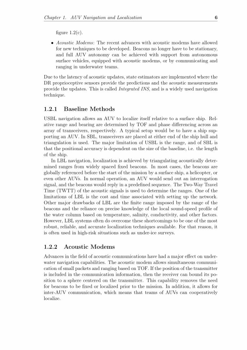
• Acoustic Modems : The recent advances with acoustic modems have allowedfor new techniques to be developed. Beacons no longer have to be stationary,and full AUV autonomy can be achieved with support from autonomoussurface vehicles, equipped with acoustic modems, or by communicating andranging in underwater teams.
Due to the latency of acoustic updates, state estimators are implemented where theDR proprioceptive sensors provide the predictions and the acoustic measurementsprovide the updates. This is called Integrated INS, and is a widely used navigationtechnique.
1.2.1 Baseline Methods
USBL navigation allows an AUV to localize itself relative to a surface ship. Rel-ative range and bearing are determined by TOF and phase differencing across anarray of transceivers, respectively. A typical setup would be to have a ship sup-porting an AUV. In SBL, transceivers are placed at either end of the ship hull andtriangulation is used. The major limitation of USBL is the range, and of SBL isthat the positional accuracy is dependent on the size of the baseline, i.e. the lengthof the ship.
In LBL navigation, localization is achieved by triangulating acoustically deter-mined ranges from widely spaced fixed beacons. In most cases, the beacons areglobally referenced before the start of the mission by a surface ship, a helicopter, oreven other AUVs. In normal operation, an AUV would send out an interrogationsignal, and the beacons would reply in a predefined sequence. The Two-Way TravelTime (TWTT) of the acoustic signals is used to determine the ranges. One of thelimitations of LBL is the cost and time associated with setting up the network.Other major drawbacks of LBL are the finite range imposed by the range of thebeacons and the reliance on precise knowledge of the local sound-speed profile ofthe water column based on temperature, salinity, conductivity, and other factors.However, LBL systems often do overcome these shortcomings to be one of the mostrobust, reliable, and accurate localization techniques available. For that reason, itis often used in high-risk situations such as under-ice surveys.
1.2.2 Acoustic Modems
Advances in the field of acoustic communications have had a major effect on under-water navigation capabilities. The acoustic modem allows simultaneous communi-cation of small packets and ranging based on TOF. If the position of the transmitteris included in the communication information, then the receiver can bound its po-sition to a sphere centered on the transmitter. This capability removes the needfor beacons to be fixed or localized prior to the mission. In addition, it allows forinter-AUV communication, which means that teams of AUVs can cooperativelylocalize.

Chapter 1. AUV Navigation and Localization 7
Popular acoustic modems are manufactured by the Woods Hole OceanographicInstitute (Woods Hole, MA, USA) [4], Teledyne Benthos (Thousand Oaks, CA,USA) [5], and EvoLogics (Berlin, Germany) [6], among others.
The ability of a modem at the surface to transmit its location to the surveyvehicles provides two important benefits over past navigation methods: 1) it re-moves the necessity to georeference the beacons before starting the mission; and2) it allows the beacons to move during the missions. The first advantage savestime and money, and the second allows the mission range to be extended as nec-essary without redeploying the sensor network. Many methods have been recentlypublished that exploits one or both of these benefits.
In some cases, certain AUVs are outfitted with more expensive sensors and/ormake frequent trips to surface for GPS position fixes. These vehicles support theother survey vehicles and have been referred to as Communication/Navigation Aids(CNAs) in the framework of Cooperative Navigation (CN). Position error will growslower if the AUVs are able to communicate their relative positions and ranges.If the CNAs (or any vehicle, for the case of homogeneous teams) surfaces for aposition fix, then the information can be shared with the rest of the team to boundthe position error.
1.3 Geophysical NavigationGeophysical navigation refers to any method that utilizes external environmentalfeatures for localization. Almost all methods in this category that achieve thebounded position error use some form of SLAM (Simultaneous Localization andMapping). Categories include the following:
• Optical : Use of a monocular or stereo camera to capture images of the seabedand then match these images to navigate.
• Sonar : Used to acoustically detect then identify and classify features in theenvironment that could be used as navigation landmarks.
Limitations for optical systems in underwater environments include the reducedrange of cameras, susceptibility to scattering, and inadequacy of lighting. As aresult, visible wavelength cameras are more commonly installed on hovering AUVsbecause they can get close to object of interest. In addition, visual odometry (theprocess of determining the vehicle pose by analyzing subsequent camera images)and feature extraction relies on the existence of features. Therefore, optical un-derwater navigation methods are particularly well suited to small-scale mapping offeature-rich environments. Examples include ship hulls or shipwreck inspections.
Sonar imaging of the ocean has become well established by decades, thereforeit is a fairly robust technology. Several types of sonars are used for seabed andstructure mapping, and they are designed to operate at specific frequencies de-pending on the range and resolution required. In all cases, the performance of theSLAM algorithm is dependent on the number and quality of the features presentin the environment. The image post-processing to detected the features for dataassociation (when required) can be done directly onboard AUVs.

Chapter 2
The CommsNet13 Experiment
Underwater navigation is still a challenging task for AUVs, requiring a trade-offbetween performance and cost. Inertial Navigation Systems (INS) of marine andnavigation grade may have an horizontal drift as limited as less than 2000 mper day, but at costs that can reach and overcome 1 Million e (unaided INS areconsidered here, i.e. inertial systems without support from additional sensors).
In the case of AUVs working in shallow water for environmental explorationand monitoring, possibly in team, there is an absolute need of keeping the cost ofany individual vehicle within reasonable bounds. As a consequence, these systemsrequire a navigation procedure able to compensate the error drift of the on-boardINS, in any.
In the framework of the THESAURUS project (Italian acronym for "TecnicHeper l’Esplorazione Sottomarina Archeologica mediante l’Utilizzo di Robot aU-tonomi in Sciami") a class of AUVs (called Typhoon) able to cooperate in swarmsto perform navigation, exploration and surveillance of underwater archaeologicalsites has been developed.
During the CommsNet13 experiment, which took place in September 2013 inthe La Spezia Gulf, North Tyrrhenian Sea, one of these vehicles was used to test amixed USBL/LBL system for navigating an AUV within a pre-specified area. TheAUV was equipped with a USBL sensor, capable also to communicate as an acousticmodem; the LBL anchors were acoustic modems deployed at the seabed in a-prioriunknown locations. The AUV was also equipped with an Inertial MeasurementUnit (IMU), and with a Global Positioning System (GPS) receiver antenna.
Conceptually, the proposed localization procedure is as follows:
• Initialization Phase: the AUV, navigating at the sea surface (knowledgeof absolute position in a standard NED frame is available thanks to GPSreceiver), interrogates repeatedly the moored modems, not necessarily fromthe same position. The measured relative positions are the transformed intoabsolute positions by exploiting the GPS information on the absolute positionof the USBL modem (i.e. the one mounted on the vehicle). The set ofmeasured absolute positions from each moored modem is averaged, in orderto obtain a final estimate of each moored modem absolute position.
• Navigation Phase: the AUV navigates with the GPS turned off, pinging themoored modems and measuring the relative position of the moored modems
8

Chapter 2. The CommsNet13 Experiment 9
Figure 2.1: Two Typhoon vehicles, the top one with standard acoustic modem andpayloads for underwater search, the bottom one with USBL modem.
with respect to the on-board USBL modem; taking into account the knowl-edge of the moored modem absolute position, the USBL modem relativeposition is transformed into an absolute position. This absolute position es-timate is fed to the navigation filter, fusing together IMU measurement andacoustic position estimates in order to reduce the drift of inertial navigation.
Section 2.1 describes the Typhoon class of vehicles, its primary design requirementsand the on-board equipment and payload. Section 2.2 illustrates the acoustic local-ization procedure previously introduced, and the results obtained are presented andbriefly discussed. Finally, Section 2.3 introduces the sound speed data recordedduring the experiment and explains how these form the basis for the followingdevelopments.
The contents of this chapter were developed using papers [7–12] as the mainreference materials.
2.1 The Typhoon Class VehiclesThe primary design requirements for the Typhoon vehicles are: maximum operat-ing depth of 250 meters; autonomy ranging from 8 to 10 hours; maximum speedof 5-6 knots1; and low cost.
Typhoon class vehicles can be divided into three different categories:
• Vision Explorer : A vehicle equipped with cameras, laser and structured lightsfor an accurate visual inspection and surveillance of archaeological sites. Vi-sual inspection involves a short range distance (few meters) between the vehi-cle and the target site, and the capability of performing precise maneuveringand hovering.
1Remember that 1 knot = 0.5 m/s.

Chapter 2. The CommsNet13 Experiment 10
• Acoustic Explorer : Preliminary exploration of extended area to recognizepotentially interesting sites involves the use of acoustic instruments, suchas side-scan sonar. This kind of vehicle can perform long range, extendedmissions. Consequently, navigation sensors able to compensate the drift ofthe inertial sensors, such as DVL, have to be installed on board.
• Team Coordinator : A vehicle with extended localization and navigation ca-pabilities is used to coordinate the team. This vehicle periodically returns tosurface providing the GPS positioning and, more generally, detailed naviga-tion information that can be shared with other vehicles of the team (this isthe approach described in Section 1.2.2).
In accordance with the project requirements, a hybrid design, able to satisfy differ-ent mission profiles, has been preferred, to reduce the engineering and productioncosts and to assure vehicles interchangeability. Each vehicle of the team can becustomized for different mission profiles (see figure 2.1).
2.1.1 The Typhoon Hardware
Typhoon vehicles are middle-sized class AUVs, whose features are comparable withother existing vehicles. The vehicle sizes are: length of about 3.6 m; externaldiameter of about 350 mm; weight of 130-180 kg according to the carried payload.
Since every vehicle can be customized to manage different payloads and missionprofiles, the system was designed by dividing the on board subsystems in two maincategories:
• Vital Systems : all the navigation, communication and safety related com-ponents and functions of the vehicle are controlled by an industrial PC-104,called Vital PC, whose functionality is continuously monitored by a watch-dog system. Most of the code implemented on the Vital PC is quite invariantwith respect to the mission profiles and payloads, assuring a high reliabilityof the system.
• Customizable Payloads : all the additional sensors and functions related tovariable payloads are managed by one or more Data PC. In particular, theData PC also manages the storage on mass memories (conventional harddisks or solid state memories) and the data coming from the connected sen-sors. This way, all the processes introduced by additional payloads are imple-mented on a platform which is also physically separated from the vital one;from an electrical point of view the two parts are protected independentlythrough fuses and relays.
For completeness here is reported a list of the on board sensors and payloads:
• Inertial Measurement Unit (IMU) Xsens MTi: device made up of a 3D gyro-scope, 3D accelerometer and 3D magnetometer furnishing dynamic data at amaximum working frequency of 100 Hz. The device measures the orientationof the vehicle in a 3D space in an accurate way thanks to an estimate innerowner algorithm.

Chapter 2. The CommsNet13 Experiment 11
J1
T1
L2
L1
L3
L4
Figure 2.2: Mission area for Sept. 22th experimental run (adapted from [7]).
• Doppler Velocity Log (DVL) Teledyne Explorer: sensor measuring the linearspeed of the vehicle, with respect to the seabed or with respect to the watercolumn beneath the vehicle. Moreover, if it detects the seabed it is also ableto measure the distance from it (like an altimeter).
• Acoustic modems (single modem or USBL-enhanced) by EvoLogics: for un-derwater communication and localization.
• Echo Sounder Imagenex 852: single beam sensor, mounted in the bow ofthe vehicle and pointing forward. It can measure the distance from the firstobstacle(s) placed in front of the vehicle.
• STS DTM depth sensor: digital pressure sensor used to measure the vehicledepth.
• PA500 echo sounder, pointing downward, to measure the vehicle elevationfrom the seabed.
• Tritech Side Scan Sonar (675 kHz) for acoustic survey of the seabed.
The reader should refer to papers [8, 9] for a more detailed description of Typhoon’shardware, propulsion system and communication network protocol.
2.2 Acoustic Localization
2.2.1 Experimental Configuration
The CommsNet13 cruise was organized and scientifically led by the NATO Science& Technology Organization Center for Maritime Research and Experimentation

Chapter 2. The CommsNet13 Experiment 12
0 50 100 150 200 250
20
40
60
80
100
120
140
160
180
200
East direction [m]
Nort
h d
irection [m
]
J1
L2
T1
Typhoon route
20 25 30 35
175
180
185
190
Figure 2.3: Initialization phase for estimating the position of the LOON modemL2 (adapted from [7]).
(CMRE), and had the broad objective of testing and comparing methodologies forunderwater communication, localization and networking. Several research institu-tions were invited to participate in the testing, that took place from Sept. 9th to22th 2013 in the Gulf of La Spezia, North Tyrrhenian Sea, and was operated fromthe R/V Alliance.
The ISME groups of the Universities of Pisa and Florence jointly participatedto the cruise bringing two Typhoon AUVs, but only the vehicle with USBL-modemcapabilities has been used in the test. The AUV has been operated from surface, tohave the availability of the GPS signal to be used as ground truth, and underwater,at a depth of almost 5-6 m.
Figure 2.2 shows the CMRE underwater network installation, named LOON,for the 22th experimental run near Palmaria Island. It consisted of four EvoLogicsacoustic modems L1, L2, L3 and L4 deployed close to the sea bottom. The referencepath for the mission consisted in the triangle (approximately 150 m per side)defined by waypoints J1, L2 (position of the second one of the four LOON modems)and T1. While navigating, the AUV was obtaining the relative position of themoored modems through its on-board USBL modem. The modems were operatedat the lowest power level allowed by the instrumentation.
More details on the experimental procedure can be found in [7].
2.2.2 Initialization Phase
Within this phase the GPS information (i.e. the AUV position in the NED absolutereference frame) is used to convert the relative position of the moored modems withrespect to the AUV body frame into the moored modems absolute position in theNED frame. Several absolute position estimates are thus obtained for each mooredmodem and, after outlier inspection and removal, the average of the measured

Chapter 2. The CommsNet13 Experiment 13
0 50 100 150 2000
20
40
60
80
100
120
140
160
180
East direction [m]
No
rth
dire
ctio
n [
m]
L2
J1
T1
1
2
3
4
5
6
GPS OFF
Typhoon programmed route
GPS
EKF (GPS on)
EKF (GPS off)
USBL fixes
(a)
0 100 200 300 400 500 6000
5
10
15
20
25
Time [s]
Err
or
[m]
Error
USBL fixes
Final Error
(b)
Figure 2.4: Estimated path and navigation error for Sept. 22th run (adapted from[7]).
positions was taken as absolute position for each moored modem, to be used assuch in the navigation phase.
Figure 2.3 shows the results for the localization of the L2 modem of the LOONnetwork. The actual position of the modem is represented by the black diamond(see enlargement), while red circles are the position measurements obtained withUSBL localization; these were averaged (after outliers removal) to obtain the po-sition estimate, represented by the red cross. This figure highlights the precisionand accuracy in acoustic measurements for this phase of the experiment.
2.2.3 Navigation Phase
Within the navigation phase, the position was estimated using: IMU measure-ments at 10 Hz rate; acoustic absolute position measurements, obtained fromthe USBL-modem relative to moored modems, and accounting for the absolutemoored modems position. Acoustic positioning data comes at irregularly spacedintervals; moreover, since the position interrogation of the modem was embeddedin a networked communication protocol, including round-robin interrogation of allthe possible modems, the delays due to such protocol were non negligible. Thecombined effect of network overburden and communication loss due to acousticchannel effects resulted in intervals between successive acoustic measurements ofthe order of tens of seconds, irregularly spaced in time throughout the experiment.
The available measurements were fused together through an Extended KalmanFilter (EKF); the filter weights were set in such a way to give more importanceto the acoustic measurements with respect to IMU measurements. For a detaileddiscussion on the filtering algorithm, see [11, 12]. Note that the AUV had no directvelocity measurements (for instance, no DVL were used.)
2.2.4 Results and Discussion
The estimated path for Sept. 22th run of the experiment is reported in figure 2.4(a),together with the GPS path, which is taken as ground truth comparison. The

Chapter 2. The CommsNet13 Experiment 14
0 50 100 150 2000
20
40
60
80
100
120
140
160
180
East direction [m]
No
rth
dire
ctio
n [
m]
L2
J1
T1
1
2
3
4
5
6
Typhoon programmed route
GPS
Delivered Pings
Failed Pings
USBL fixes
(a)
0 50 100 150 200
0
20
40
60
80
100
120
140
160
180
East direction [m]
No
rth
dire
ctio
n [
m]
L2
J1
T1
1 2
3 4
5 6 7
8
9
10
11
Typhoon programmed route
EKF
Delivered Pings
Failed Pings
USBL fixes
(b)
Figure 2.5: Acoustic performance of the LOON installation for two Sept. 22th runs(adapted from [7]).
red diamonds in the figure indicates the acoustic position measurements. In fig-ure 2.4(b) we also report the estimation error, computed as the distance (norm) inmeters between the filter estimated position and the GPS position as a functionof time. The diamonds represent the instant in time in which an acoustic positionmeasurement is received by the filter.
From both figures it can be noted the expected drift in position estimate inthe absence of acoustic measurements data (when navigation relies on IMU deadreckoning only), and how the acoustic position fixes are effective in decreasing thenavigation error. As an additional consideration, it is notable how the intervalin time between two successive measurements can indeed be of minute scale. Asalready commented, there are two significant sources of delay in this setup: oneis the communication structure, the other is the variability of the channel withconsequent loss of position messaging.
Figure 2.5 shows the spatial distribution of the modem interrogations: in par-ticular, the green circles and the red crosses indicate the position of the vehicle atthe time instant of an acoustic ping, respectively successful or not. A new USBLmeasurement, indicated by the red diamond, occurs as a result of a delivered ping;however, it is evident that not all the successful interrogations provide a positioninginformation. As can be expected, the acoustic communication is strongly depen-dent on the vehicle position at the moment of the interrogation. This correlationbetween transmission successes/failures and the position of the vehicle suggestedus to collect environmental data and further investigate how the acoustic channel(whose properties change with position) influences signal propagation.
2.3 Recorded Sound Speed DataFigure 2.6 depicts the underwater sound speed data recorded using a CTD sensorin the Gulf of La Spezia on the Sept. 14th experimental run, both for morningand afternoon periods of the day. Sound speed is the most important parameterin ocean acoustics (as we will see extensively in Chapter 3), and CTD sensors are

Chapter 2. The CommsNet13 Experiment 15
1515 1520 1525 1530 1535
0
5
10
15
20
25
30
Sound Speed (m/s)
Dep
th (
m)
(a)
1515 1520 1525 1530 1535
0
5
10
15
20
25
30
Sound Speed (m/s)
Dep
th (
m)
(b)
Figure 2.6: Sound speed profiles recorded during CommsNet13 sea trials on Sept.14th run.
oceanographic instruments used to determine the conductivity, temperature anddepth of the ocean2. As we can see, morning and afternoon profiles are very similar.They both possess a strong negative gradient near the sea bottom, and the onlydifference is in the upper part (constant for morning, linear for afternoon), that isvery sensitive to atmospheric and climatic factors.
These data were chosen as representatives of the acoustic environmental condi-tions during CommsNet13 trials. As previously stated, one of the possible causesof the irregularly time-spaced acoustic fixes relies in the communication losses be-tween the moored modems and the AUV due to acoustic channel effects. Sincesound speed completely characterizes the channel properties (together with waterand sea bottom geoacoustic parameters), the data pictured in figure 2.6 can be usedto analyze the transmission quality between the moored modems and the movingUSBL-vehicle, to better optimize the geometry of communication and therefore topossibly increase the reliability of acoustic fixes. This is precisely the main focusof the remaining chapters of this thesis.
2The reader should refer to [13] for an introduction on CTDs.

Chapter 3
Underwater Acoustics Fundamentals
The aim of this chapter is to introduce the unfamiliar reader to the basic concepts ofunderwater acoustics, in order to understand how computational methods work andto interpret the developments and the results provided in the following chapters.
Section 3.1 contains a brief summary of the main oceanographic physical quan-tities (especially sound speed), and how they influence sound propagation underwa-ter. Acoustical properties of the ocean environment and the seabed are describedtoo.
Section 3.2 presents some characteristic propagation paths of sound waves inunderwater environments. Using the ray theory formalism, wave paths are a directconsequence of Snell’s Law, which relates the ray angle to the local sound speed.If the speed of sound is not constant, the rays will follow curved paths rather thanstraight ones, and this has a great impact on sonar coverage and source-receivertransmissions.
Section 3.3 introduces the theory of acoustic waves. The wave equation influids is formulated both in the time and frequency domains, and the principle ofreciprocity is stated. The former is the basis for the numerical methods describedin Chapter 4, the latter is of fundamental practical importance in wave phenomenaand linear systems.
The contents of this chapter were developed using books [14, 15] as the mainreference materials. For a complete treatment on ocean acoustics, the reader shouldalso refer to [16, 17].
3.1 The Underwater Acoustic Environment
3.1.1 Oceanographic and Physical Properties
The ocean is an acoustic waveguide limited above by the sea surface and belowby the seafloor. The speed of sound (c) in the waveguide is the most importantquantity and is normally related to density and compressibility. The sound speedis given by the square root of the ratio between volume stiffness (or bulk modulus)and density:
c =
√K
ρ. (3.1)
16
Chapter 3. Underwater Acoustics Fundamentals 17
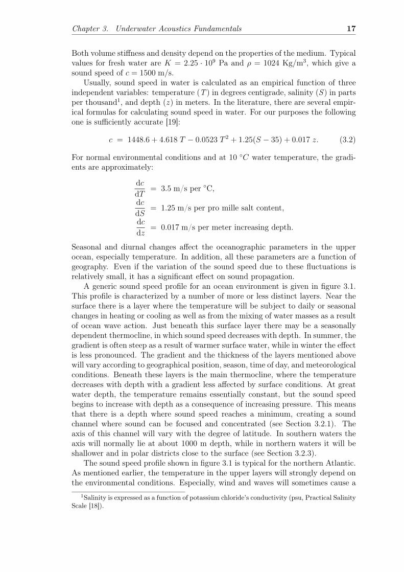
Both volume stiffness and density depend on the properties of the medium. Typicalvalues for fresh water are K = 2.25 · 109 Pa and ρ = 1024 Kg/m3, which give asound speed of c = 1500 m/s.
Usually, sound speed in water is calculated as an empirical function of threeindependent variables: temperature (T ) in degrees centigrade, salinity (S ) in partsper thousand1, and depth (z ) in meters. In the literature, there are several empir-ical formulas for calculating sound speed in water. For our purposes the followingone is sufficiently accurate [19]:
c = 1448.6 + 4.618 T − 0.0523 T 2 + 1.25(S − 35) + 0.017 z. (3.2)
For normal environmental conditions and at 10 ◦C water temperature, the gradi-ents are approximately:
dc
dT= 3.5 m/s per ◦C,
dc
dS= 1.25 m/s per pro mille salt content,
dc
dz= 0.017 m/s per meter increasing depth.
Seasonal and diurnal changes affect the oceanographic parameters in the upperocean, especially temperature. In addition, all these parameters are a function ofgeography. Even if the variation of the sound speed due to these fluctuations isrelatively small, it has a significant effect on sound propagation.
A generic sound speed profile for an ocean environment is given in figure 3.1.This profile is characterized by a number of more or less distinct layers. Near thesurface there is a layer where the temperature will be subject to daily or seasonalchanges in heating or cooling as well as from the mixing of water masses as a resultof ocean wave action. Just beneath this surface layer there may be a seasonallydependent thermocline, in which sound speed decreases with depth. In summer, thegradient is often steep as a result of warmer surface water, while in winter the effectis less pronounced. The gradient and the thickness of the layers mentioned abovewill vary according to geographical position, season, time of day, and meteorologicalconditions. Beneath these layers is the main thermocline, where the temperaturedecreases with depth with a gradient less affected by surface conditions. At greatwater depth, the temperature remains essentially constant, but the sound speedbegins to increase with depth as a consequence of increasing pressure. This meansthat there is a depth where sound speed reaches a minimum, creating a soundchannel where sound can be focused and concentrated (see Section 3.2.1). Theaxis of this channel will vary with the degree of latitude. In southern waters theaxis will normally lie at about 1000 m depth, while in northern waters it will beshallower and in polar districts close to the surface (see Section 3.2.3).
The sound speed profile shown in figure 3.1 is typical for the northern Atlantic.As mentioned earlier, the temperature in the upper layers will strongly depend onthe environmental conditions. Especially, wind and waves will sometimes cause a
1Salinity is expressed as a function of potassium chloride’s conductivity (psu, Practical SalinityScale [18]).

Chapter 3. Underwater Acoustics Fundamentals 18
Figure 3.1: Typical sound speed profile as a function of depth for an ocean envi-ronment (adapted from [14]).
total mixing of the water masses, making the water temperature almost constantin the surface layer. In such a mixed layer with constant temperature, sound speedwill have a small positive gradient because of the depth.
Turning to the upper and lower boundaries of the ocean waveguide, the seasurface is a simple horizontal boundary and a nearly perfect reflector. The seafloor,on the other hand, is a lossy boundary with strongly varying topography acrossocean basins (see Section 3.1.3).
3.1.2 Relevant Units in Ocean Acoustics
Underwater acoustic signals are compressional waves (or longitudinal waves) prop-agating in a fluid medium, in which the displacement of the medium is in the samedirection as, or the opposite direction to, the direction of travel of the wave2. Themain physical quantities that characterize this type of wave are pressure (whichis a function of space and time), expressed in pascals (Pa = N/m2), and inten-sity, expressed in W/m2; the latter is defined as the average rate of flow of energythrough a unit area that is normal to the direction of propagation, and it has thefollowing expression:
I =p2rmsZ
, (3.3)
where prms is the root mean square sound pressure, i.e. the squared integral ofinstantaneous pressure over a time period T , and Z = ρc is the acoustic impedance
2There are also transverse waves, or shear waves, in which the displacement of the medium isperpendicular to the direction of propagation of the wave.

Chapter 3. Underwater Acoustics Fundamentals 19
of the medium, measured in Kg/(m2s). For seawater, Z is 1.5 · 106 Kg/(m2s).The decibel (dB) is the dominant adimensional unit in underwater acoustics
and denotes a ratio of intensities expressed in terms of a logarithmic (base 10)scale:
10 log(I1I2
)= 20 log
(p1p2
), (3.4)
where the transition from intensities to rms pressures assumes that the acousticimpedance doesn’t change (so that the intensity in a plane wave becomes propor-tional to the square of the pressure amplitude). Absolute intensities can thereforebe expressed by using a reference intensity. The presently accepted reference in-tensity I0 is the intensity of a plane wave having a prms equal to 1 µPa = 10−6 Pa;therefore, in seawater, we have I0 = 0.67 · 10−18 W/m2 (i.e. 0 dB re 1µPa).
An acoustic signal traveling through the ocean becomes distorted due to multi-path effects and weakened due to various loss mechanisms. The standard measurein underwater acoustics of the change in signal strength with range is transmissionloss (TL) defined as the ratio in decibels between the acoustic intensity I(r, z) ata field point and the intensity I0 at 1-m distance from the source:
TL = −10 log(I(r, z)
I0
)= −20 log
(|p(r, z)||p0|
)dB re 1 m,
(3.5)
where the minus sign makes it positive, since I(r, z) < I0. Again, the last equationassumes that the acoustic impedance at the field point is the same as that at thesource, assumption that will remain valid throughout this document.
Transmission loss may be considered to be the sum of a loss due to geometricalspreading and a loss due to attenuation. The spreading loss is simply a measure ofthe signal weakening as it propagates outward from the source. It can be of twotypes:
• Spherical spreading loss, when the power radiated by the source is equallydistributed over the surface area of a sphere surrounding the source;
• Cylindrical spreading loss, when the medium has plane upper and lowerboundaries.
For a point source in a waveguide with depth D and range r, we have sphericalspreading in the nearfield (r ≤ D) followed by a transition region toward cylindricalspreading which applies only at longer ranges (r � D).
During their propagation, acoustic waves will also encounter losses caused byviscosity, thermal conductance, and different relaxation phenomena. Ultimately,the acoustic energy is lost to heat due to the interaction of the particles of themedium caused by the waves. A very important parameters is the absorptioncoefficient (or attenuation coefficient) α, which is defined from a decay-law-typedifferential equation in theoretical acoustics:
dA
dx= −α⇒ A = A0e
−αx, (3.6)

Chapter 3. Underwater Acoustics Fundamentals 20
p ρb/ρw cp/cw cp cs αp αsBottom Type (%) - - (m/s) (m/s) dB/λp dB/λsClay 70 1.5 1.00 1500 <100 0.2 1.0Silt 55 1.7 1.05 1575 150 1.0 1.5Sand 45 1.9 1.10 1650 300 0.8 2.5Gravel 35 2.0 1.20 1800 500 0.6 1.5Moraine 25 2.1 1.30 1950 600 0.4 1.0Chalk - 2.2 1.60 2400 1000 0.2 0.5Limestone - 2.4 2.00 3000 1500 0.1 0.2Basalt - 2.7 3.50 5250 2500 0.1 0.2
cw = 1500 m/s, ρw = 1000 kg/m3
Table 3.1: Geoacoustic properties for sediments and other materials.
where A0 is the rms amplitude of the wave at x = 0. This coefficient is a functionof frequency and it is usually expressed in dB/km or dB/λ (λ is the wavelength).
A quantitative understanding of acoustic loss mechanisms in the ocean is re-quired for the modeling of sound propagation. The most important loss mecha-nisms are volume attenuation, bottom reflection loss, and boundary and volumescattering. For a complete treatment of these mechanisms, see [14, pagg. 35-57].
3.1.3 Sound Speed in Marine Sediments
When sound interacts with the seafloor, the structure of the ocean bottom becomesimportant. Ocean bottom sediments are often modeled as fluids, which means thatthey support only one type of sound wave - a compressional wave. This is oftena good approximation since the rigidity of the sediment is usually considerablyless than that of a solid, such as rock. In the latter case, which applies to theocean basement or the case where there is no sediment overlying the basement, themedium must be modeled as elastic, which means it supports both compressionaland shear waves3.
A geoacoustic model is defined as a model of the real seafloor with emphasison measured, extrapolated, and predicted values of those material properties im-portant for the modeling of sound transmission. The information required for acomplete geoacoustic model should include at least the following depth-dependentmaterial properties: the compressional wave speed cp, the shear wave speed cs,the compressional wave attenuation αp, the shear wave attenuation αs, and thedensity ρ. Moreover, information on the variation of all of these parameters withgeographical position is required.
The geoacoustic properties of some typical seafloor materials are listed in ta-ble 3.1. Several observations can be made. First, we see that the porosity p relatesin a simple fashion to the material density and the wave speed, i.e. a lower poros-ity results in a higher density and higher wave speeds. Next, the shear speeds inunconsolidated sediments (clay, silt, sand, gravel) increase rapidly with depth be-
3In reality, the media are viscoelastic, meaning that they are also lossy.

Chapter 3. Underwater Acoustics Fundamentals 21
low the water-bottom interface4. Wave attenuations α are generally given in unitsof dB per wavelength, indicating that the attenuation increases linearly with fre-quency. Bottom materials are three-to-four orders of magnitude more lossy thanseawater. It must be emphasized that these values are merely indicative. Thevastly different material compositions and stratifications encountered in the oceanseafloors essentially mean that a specific geoacoustic model must be establishedfor any given (small or large) geographical area. Clearly, the construction of adetailed geoacoustic model for a particular ocean area is a tremendous task, andthe amount of approximate (or inaccurate) information included is the primarylimiting factor on the accurate modeling of bottom-interacting sound transmissionin the ocean.
3.2 Underwater Sound PropagationAll the typical sound paths resulting from various sound speed profiles can beunderstood from Snell’s Law, which states that:
cos θ
c= const, (3.7)
and relates the ray angle (w.r.t. the horizontal) θ to the local sound speed c.It is quite straightforward to see that the implication of this law is that soundbends locally towards regions of low sound speed: if c increases, θ must decreaseto compensate the variation, and vice versa.
In this section we are going to describe four typical environmental situationsand characteristic paths: deep sound channel, convergence-zone, arctic propagationand shallow waters. We must remember that the modeling of sound propagation iscomplicated because the environment varies laterally (it is range dependent) and allenvironmental effects on sound propagation are dependent on acoustic frequencyin a rather complicated way.
3.2.1 Deep Sound Channel
As we can see from figure 3.2, the principal characteristic of standard deep-waterpropagation is the existence of an upward-refracting sound-speed profile which per-mits long-range propagation without significant bottom interaction (deep soundchannel). Typical deep-water environments are found in all oceans at depths ex-ceeding 2000 m.
Propagation in the deep sound channel, also referred to as the SOFAR channel,allows long-range propagation without encountering reflection losses at the seasurface or the seafloor. Because of the low transmission loss, acoustic signals in thedeep sound channel have been recorded over distances of thousands of kilometers.
The sound channel axis (minimum sound speed) varies in depth from around1000 m at mid-latitudes to the ocean surface in polar region; a necessary conditionfor the existence of low-loss refracted paths is that the sound-speed axis is below
4Shear speeds in sediments are therefore most appropriately given in terms of their depthdependence.

Chapter 3. Underwater Acoustics Fundamentals 22
Figure 3.2: Deep sound channel propagation (adapted from [14]).
Figure 3.3: Convergence-zone propagation (adapted from [14]).
the sea surface, since otherwise propagation becomes entirely surface-interactingand lossy (see Section 3.2.3).
3.2.2 Convergence Zones
The acoustic field pattern shown in figure 3.3 is one of the most interesting fea-tures of propagation in the deep ocean. The presence of two sound channel axes(a sort of double SOFAR) determines a new propagation path. This pattern isreferred to as convergence-zone (CZ) propagation because the sound emitted froma near-surface source forms a downward-directed beam which, after following adeep refracted path in the ocean, reappears near the surface to create a zone ofhigh sound intensity (convergence or focusing) at a distance of kilometers fromthe source. The phenomenon is repetitive in range, with the distance between the

Chapter 3. Underwater Acoustics Fundamentals 23
Figure 3.4: Arctic environment propagation (adapted from [14]).
high-intensity regions called the convergence-zone range.The importance of convergence-zone propagation stems from the fact that it
allows for long-range transmission of acoustic signals of high intensity and lowdistortion. The convergence zones are spaced approximately 65 km apart, notealso that the convergence zone width increases with zone number; the second zoneis wider than the first, and so on, until eventually at several hundreds kilometersthe zones overlap and become indistinguishable.
The paper [20] was the first to address in detail the environmental conditionsfor the existence of convergence zones and attempted a theoretical description ofthe convergence-zone structure using ray theory.
3.2.3 Arctic Propagation
Propagation in the Arctic Ocean (figure 3.4) is characterized by an upward re-fracting profile over the entire water depth causing energy to undergo repeatedreflections at the underside of the ice. The sound speed profile in these regions canoften be approximated by two linear segments with a steep gradient in the upper200 m caused both by the increase in temperature and in salinity with depth.
The ray diagram in figure 3.4 shows that energy is partly channeled beneaththe ice cover within the 200 m deep surface duct (since minimum sound speed isat the surface) and partly follows deeper refracted paths. All rays within a coneof almost ±17◦ propagate to long ranges without bottom interaction. This typeof propagation is known to degrade rapidly with increasing frequency above 30 Hz(for more details see [17]).
3.2.4 Shallow Waters
The principal characteristic of shallow waters propagation is that the sound speedprofile is downward refracting or nearly constant over depth, meaning that long-range propagation takes place exclusively via bottom-interacting paths (as one

Chapter 3. Underwater Acoustics Fundamentals 24
Figure 3.5: Shallow waters propagation (adapted from [14]).
would expect). Typical shallow waters environments are found on the continentalshelf for water depths down to 200 m.
Accurate prediction of long-range propagation in shallow waters is a very com-plex problem. In shallow waters the surface, volume and bottom properties areall important, are spatially and temporally varying, and the parameters are gener-ally not known in sufficient detail and with enough accuracy to permit long-rangepredictions in a satisfactory way.
A ray picture of propagation in a 100 m deep shallow waters duct is shownin figure 3.5. The sound speed profile is typical of the Mediterannean Sea in thesummer. There is a warm surface layer causing downward refraction and hencerepeated bottom interaction for all ray paths. The seasonal variation in soundspeed structure is significant with winter conditions being nearly isospeed. Theresult is that there is less bottom interaction in winter than in summer, whichmeans that propagation conditions are generally better in winter than in summer.
To better examine transmission loss variability in shallow water propagation,see [14, pagg. 28-32].
3.3 Acoustic Waves TheoryAcoustic waves are mechanical vibrations. When an acoustic wave passes througha medium, it causes local density changes that are related to local displacementsof mass about the rest positions of the particles in the medium. This displacementleads to the formation of forces that act to restore the density to the equilibriumstate and move the particles back to their rest positions. The medium may bea gas, liquid, or solid material. The basic equations of acoustics are obtained byconsidering the equations for an inviscid and compressible fluid. These equationsare expressed with the notation that p is the pressure, ρ is density, S is entropy,and v is particle velocity (bold face letters denote vectors).
3.3.1 Derivation of the Wave Equation
We now formulate the wave equation describing acoustic waves in fluids, usingthree simple principles:

Chapter 3. Underwater Acoustics Fundamentals 25
• The momentum equation, also known as Euler’s equation.
• The continuity equation, or conservation of mass.
• The equation of state: the relationship between changes in pressure anddensity or volume.
We consider a small rectangular volume element with sides dx, dy and dz, volumeV = dx dy dx and mass ρV , with ρ being the density of the fluid. As a result ofthe acoustic wave action, mass will alternately flow into and out of the elementwith displacement velocity, or particle velocity, v = [vx vy vz], depending on theposition of the element and the time.
Conservation of mass implies that the net changes in the mass, which resultfrom its flow through the element, must be equal to the changes in the density ofthe mass of the element. This is expressed by the continuity equation:
∂ρ
∂t= −∇ · (ρv). (3.8)
Equation (3.8) is nonlinear since it contains the product of density and particlevelocity, both being functions of time and position.
The second fundamental equation is Euler’s equation (or momentum balance):
ρ
[∂v
∂t+ v · ∇v
]= −∇p, (3.9)
and it is an extension of Newton’s second law, which states that force equals theproduct of mass and acceleration. The extension is the second left-hand term inequation (3.9), which represents the change in velocity with position for a giventime instant, while the first term describes the change with time at a given position.
Finally, an equation of state is required to give a relationship between a changein density and a change in pressure, taking into consideration the existing ther-modynamic conditions. The equation of state may be formulated as pressure as afunction of density and entropy S:
p = p(ρ, S)⇒ p = p(ρ). (3.10)
In a real fluid, the dissipation processes like viscosity and thermal conduction actto increase the entropy, as demanded by the second law of thermodynamics. Theincrease in entropy is associated with heating of the fluid as the sound wave passesand a corresponding decrease in the energy of the sound wave. The effect of anincrease of entropy leads naturally to the idea of attenuation of the sound.
Equations (3.8) to (3.10) can be linearized by assuming that each physical quan-tity is a function of a steady state, time-independent value and a small fluctuationterm:
p = p0 + p′,
ρ = ρ0 + ρ′, (3.11)v = v0 + v′.

Chapter 3. Underwater Acoustics Fundamentals 26
The variables p′, ρ′ and v′ are functions of time and spatial positions; the variablesp0, ρ0 and v0 are independent of time, but may be functions of spatial positions.We also assume that there is also no mean flow, that is, v0 = 0. We expandequation (3.10) about the equilibrium values, indicated by the subscript 0, andobtain:
p = p0 +
[∂p
∂ρ
]0
(ρ− ρ0) +1
2
[∂2p
∂ρ2
]0
(ρ− ρ0)2 + . . . (3.12)
Using equations (3.11) and (3.12), after some passages5 and assuming that nominaldensity ρ0 is constant in space, we obtain the acoustic wave equation for soundpressure:
∇2p′ − 1
c20
∂2p′
∂t2= 0, (3.13)
where ∇2 is the Laplacian operator and c0 is the sound speed at the ambientconditions, calculated from equation (3.1).
Other variables, such as particle velocity, also must satisfy the same wave equa-tion. For instance, the wave equation for particle velocity v is
∇(∇ · v)− 1
c20
∂2v
∂t2= 0. (3.14)
Generally, it is more convenient to describe the wave by means of scalar variables.Denoting the velocity potential as φ, the particle velocity is expressed by the gra-dient of the velocity potential φ as:
v = ∇φ. (3.15)
By combining equation (3.15) with equation (3.14), we find that the velocity po-tential satisfies the wave equation:
∇2φ− 1
c20
∂2φ
∂t2= 0. (3.16)
It follows that the sound pressure is equal to:
p = −ρ0∂φ
∂t. (3.17)
Equations (3.15) to (3.17) are the ones generally applied in further treatments ofwave propagation.
The wave equations that were formulated hitherto may be referred to as homo-geneous wave equations because they lack a source term. Introduction of a sourceterm leads to the inhomogeneous wave equations. A source can be an external forceor an injection of a volume of fluid (i.e. injection of new mass into the medium).The pressure wave equation with a volume source term is expressed as:
∇2p′ − 1
c20
∂2p′
∂t2= ρ0
∂f(r, t)
∂t, (3.18)
where f(r, t) is the forcing term for a source located at r, and the velocity potentialequation becomes:
∇2φ− 1
c20
∂2φ
∂t2= −f(r, t). (3.19)
5For all the details see [15, pagg. 16-18].

Chapter 3. Underwater Acoustics Fundamentals 27
3.3.2 The Helmholtz Equation
We can move from time domain to frequency domain by using the Fourier trans-form:
Φ(ω) =
∫ +∞
−∞φ(t)eiωt dt, (3.20)
and back to time domain by using the inverse transform:
φ(t) =1
2π
∫ +∞
−∞Φ(ω)e−iωt dω. (3.21)
Analysis in the frequency domain means that we assume a solution of the waveequation in the form Φ(ω)exp(iωt). After this solution is found, the solution in thetime domain, and consequently the time response, is found by using the inversetransformation in equation (3.21).
The inhomogeneous wave equation for the velocity potential may then be ex-pressed as: [
∇2 + κ2(r)]Φ(r, ω) = −F (r, ω), (3.22)
where F (r, ω) is the Fourier transform of f(r, t) defined in equation (3.18), andthe wave number κ(r) is defined as:
κ(r) =ω
c0(r). (3.23)
Equation (3.22) is the wave equation in the frequency domain and is also referredto as the inhomogeneous Helmholtz equation, which is often easier to solve than thecorresponding wave equation in the time domain due to the reduction in the di-mension of this PDE (partial differential equation). This simplification is achievedat the cost of having to evaluate the inverse Fourier transform (3.21).
The Helmholtz equation, rather than the wave equation, form the theoreticalbasis for the most important numerical methods in computational acoustics, includ-ing Wavenumber Integration (WI), Normal Modes (NM) and Parabolic Equations(PE) [14]. In spite of the relative simplicity of equation (3.22), there is no universalsolution technique available. The solution technique that can be applied dependson the following factors:
• Dimensionality of the problem.
• Medium wavenumber variation κ(r), i.e. the sound speed variation c(r).
• Boundary conditions.
• Source-receiver geometry.
• Frequency and bandwidth.

Chapter 3. Underwater Acoustics Fundamentals 28
3.3.3 The Principle of Reciprocity
Reciprocity is a fundamental principle related to wave propagation and to linearsystems in general. It is therefore of great practical importance. Applied to wavepropagation, the reciprocity principle enables us to switch the positions of sourceand receiver and still receive the same acoustic signal.
Let’s consider an ideal experimental situation with transmission of sound be-tween two positions indicated by A and B. In one experiment sound is transmittedfrom A by a small spherical sound source with strength6 QA and we measure thesound pressure pB in position B. Another experiment uses a source at position Bwith strength QB and we receive the pressure pA at position A.
The reciprocity principle states that the ratios of source strengths and receivedpressures are the same, as expressed by the following relationship:
QA
pB=
QB
pA. (3.24)
Equation (3.24) is very general and applies as long as the sources have the samefrequency. The equation constitutes the reciprocity principle: the pressure at posi-tion B due to a source at position A is equal to the pressure at A due to a similarsource at position B. This result holds also for the case where the medium iscomposed of several regions, and in cases where the wave undergoes reflections andrefractions on its path from A to B or vice versa.
6The source strength Q(ω) is the Fourier transform of the source function in equation (3.19)[15].
Chapter 4
Sound Propagation Models
Sound propagation in the ocean is mathematically described by the wave equa-tion, whose parameters and boundary conditions are representative of the oceanenvironment. There are essentially five types of models (computer solutions to thewave equation) to describe sound propagation in the sea: spectral or "fast fieldprogram" (FFP), normal modes (NM), ray tracing and parabolic equation (PE)models, and direct finite-difference (FDM), or finite element (FEM) solutions tothe full wave equation. All of these models permit the ocean environment to varywith depth; a model that also permits horizontal variations in the environmentis termed range dependent. The major difference between the various techniquesis the mathematical manipulation of equation (3.19) being applied before actualimplementation of the solution, another difference is the form of the wave equationused.
FDM and FEM are the most direct, general approaches, but their importancein ocean acoustics is rather limited due to excessive computational requirements.The alternative numerical approaches (FFP, NM, PE and rays) are much moretractable in term of numerical requirements and are therefore in more widespreaduse in the ocean acoustics community. However, the improved efficiency is obtainedat the cost of generality. All these approaches are based on assumptions allowingfor simplifying mathematical manipulations of the wave equation.
This chapter describes one of these models, ray tracing (Section 4.1), whichwas used to produce all the acoustic channel simulations shown in this thesis. Sec-tion 4.2 is a brief summary of the available software that implements this method.
The contents of this chapter were developed using books [14, 15], together with[21, 22], as the main reference materials.
4.1 Ray MethodsRay acoustics and ray-tracing techniques are the most intuitive and often thesimplest means for modeling sound propagation in the sea. Ray acoustics is basedon the assumption that sound propagates along rays that are normal to wave fronts,surfaces of constant phase of the acoustic waves. The computational techniqueknown as ray tracing is a method used to calculate the trajectories of the raypaths of sound from the source.
29

Chapter 4. Sound Propagation Models 30
The ray theory approach is essentially a high-frequency approximation, ap-plicable to frequencies for which the wavelength is much smaller than the waterdepth and, in addition, much smaller than the characteristic distance of variationin the sound speed. This method is sufficiently accurate that it is used in appli-cations involving echo sounders, sonar, and communication systems for short andmedium-short distances. These devices normally use frequencies that satisfy thehigh-frequency conditions.
Ray theory gives a good physical picture of how sound propagates in inho-mogeneous media. An advantage of ray theory is that ray characteristics are notfunctions of frequency and therefore are very efficient for modeling propagationof broadband time signals. Section 4.1.1 introduces ray acoustics theory, which isthe fundamental basis upon which practical implementations are built, while Sec-tion 4.1.2 describes the differences between coherent and incoherent transmissionloss, which is a fundamental distinction for this kind of methods. Section 4.1.3 listssome of the typical artifacts and issues that can be encountered in ray acoustics.
4.1.1 Theory of Ray Acoustics
The wave equation for the velocity potential in rectangular (or cartesian) coordi-nates x = (x, y, z) may be written as:
∇2φ(x, y, z, t) =1
c2(x, y, z)
∂2φ(x, y, z, t)
∂t2. (4.1)
We assume a solution of the form:
φ(x, y, z, t) = A(x, y, z)exp[−iω
(t− W (x, y, z)
c0
)], (4.2)
where A(x, y, z) is the position-dependent amplitude and c0 is a reference soundspeed. The function W (x, y, z) represents the wave fronts because all points inspace where W (x, y, z)− c0t is a constant have the same phase, as can be seen byexamining the exponential in equation (4.2).
Inserting equation (4.2) into the wave equation (4.1), and requiring the waveequation to be satisfied independently for both the real and the imaginary partsresults in two equations from which we can determine W (x, y, z) and A(x, y, z):
∇2A− Aω2
c20∇W · ∇W = −Aω
2
c2, (4.3)
2∇A · ∇W + A∇2W = 0. (4.4)
So far, no assumptions have been made, and in principle we can solve these twodifferential equations, thereby finding a complete solution for wave equations thathave three-dimensional variation in the sound speed c(x, y, z). This approach isoften referred to as exact ray tracing. In practice, this approach is very difficultbecause equations (4.3) and (4.4) are nonlinear and coupled. Therefore some sim-plifying assumptions must be introduced. If we assume that:
∇2A� Aω2
c2, (4.5)

Chapter 4. Sound Propagation Models 31
the second term on the left side of equation (4.3) dominates, and the first term canbe neglected. This mean that the wave front W must satisfy the equation:
∇W · ∇W =(c0c
)2, (4.6)
which can be rewritten as:∇W 2 = n2. (4.7)
Here, the index of refraction n is defined as:
n =c0c. (4.8)
Equation (4.7), the so called eikonal equation, is a first-order nonlinear differen-tial equation; it gives the geometry for the spatial variation of the wave frontW (x, y, z, t). Equation (4.4), the transport equation, gives the sound field ampli-tude as a function of spatial position.
Two conditions must be satisfied for the assumption made in equation (4.5) tobe valid. First, the frequency must be sufficiently high that any variation in thesound speed over a distance equal to a wavelength is vanishingly small; this is thereason why ray methods are rarely applied to low-frequency problems. Second, thespatial variation of the amplitude must be small, which means that equation (4.5)will not be satisfied at the edges of a sound field. A consequence of this secondcondition is that diffraction effects are not well represented by the ray approxima-tion.
We now continue with the eikonal equation to calculate the trajectories of theray paths. We first define the unit vector e normal to the wave front W (x, y, z, t);from equation (4.7), we find that:
∇W = ne. (4.9)
Although the solution of this equation defines the ray path direction at any pointon the trajectory, it is more convenient to work with the ray path coordinatess(x, y, z), which determine the ray direction e by:
e =ds
ds= i
dx
ds+ j
dy
ds+ k
dz
ds, (4.10)
where dx/ ds, dy/ ds and dz/ ds are the direction cosines of the ray and have theproperty: (
dx
ds
)2
+
(dy
ds
)2
+
(dz
ds
)2
= 1, (4.11)
where s is the distance measured along the ray path.The direction numbers for the normal to the phase front of W (x, y, z, t) are
∂W/∂x, ∂W/∂y and ∂W/∂z for the x, y and z directions, respectively. These areproportional to the direction cosines and the proportionality may be expressed by

Chapter 4. Sound Propagation Models 32
three equations:
dx
ds= a
dW
dx,
dy
ds= a
dW
dy, (4.12)
dz
ds= a
dW
dz.
The value of a, after some passages, is found to be equal to 1/n, therefore equations(4.12) become:
dx
ds=
1
n
dW
dx,
dy
ds=
1
n
dW
dy, (4.13)
dz
ds=
1
n
dW
dz.
To find the equation describing the ray path s(x, y, z), we must eliminateW (x, y, z, t)by taking the differential d/ ds along the path. For the x-component, this produces:
d
ds
(n
dx
ds
)=
d
ds
(∂W
∂x
)=
∂
∂x
[∂W
∂x
dx
ds+∂W
∂y
dy
ds+∂W
∂z
dz
ds
]. (4.14)
By using equations (4.7) and (4.11), this expression can be written as:
d
ds
(n
dx
ds
)=
∂n
∂x. (4.15)
After similar treatment of the y- and z-components, we obtain:
d
ds
(n
dx
ds
)=
∂n
∂x,
d
ds
(n
dy
ds
)=
∂n
∂y, (4.16)
d
ds
(n
dz
ds
)=
∂n
∂z.
In electromagnetics and optics, the speed of light in a vacuum is a fundamentalquantity and thus is a natural choice for the reference speed c0. In acoustics,there is no such fundamental reference speed. Therefore equation (4.16) is oftenexpressed by using the sound speed as:
d
ds
(1
c
dx
ds
)= − 1
c2∂c
∂x,
d
ds
(1
c
dy
ds
)= − 1
c2∂c
∂y, (4.17)
d
ds
(1
c
dz
ds
)= − 1
c2∂c
∂z.

Chapter 4. Sound Propagation Models 33
Equations (4.16) and (4.17) are ordinary differentials equations that describe howto compute ray trajectories in the general case where the sound speed c(x, y, z)varies with all three spatial coordinates. In practice, this form is rarely usedbecause of its complexity and the lack of detailed knowledge about the soundspeed in the horizontal directions.
The next approximation involves assumption of transverse isotropy (TI), whichmeans the sound speed may vary with depth z and range r, but not with azimuth.This assumption is also justified physically because the gradients in the oceanvariables that affect sound speed (temperature and salinity) are much greater indepth than in x and y, as discussed in Section 3.1.1.
In this case we have cylindrical symmetry around the z axis and we thereforeuse cylindrical coordinates. A small segment of a ray path ds has horizontal andvertical components dr and dz, respectively, and forms an angle (often called graz-ing angle) of θ with respect to the horizontal. With this cylindrical coordinates, wealso introduce two new variables, called the ray parameters, ξ(s) and ζ(s), definedas:
ξ(s) =1
c
dr
ds=
1
ccos θ,
ζ(s) =1
c
dz
ds=
1
csin θ.
(4.18)
Parameters ξ(s) and ζ(s) are proportional to the horizontal (k) and vertical (γ)wavenumber components, respectively, that is:
k = ωξ,
γ = ωζ.(4.19)
By equations (4.17), the wavenumber components satisfy the differential equations:
dξ
ds= − 1
c2∂c
∂r,
dζ
ds= − 1
c2∂c
∂z.
(4.20)
Using equation (4.18), we find that the initial values for integrating those equationsare:
ξ =cos θ0c(r0, z0)
,
ζ =sin θ0c(r0, z0)
.
(4.21)
where θ0 is the ray angle and c(r0, z0) is the sound speed at the starting point(r0, z0).
Equations (4.20) determine the change in ray path direction as the sound speedchanges with both range and depth. These equations are therefore the basis forray tracing in a range dependent environment, where the sound speed is a functionof both range and depth. In principle, equations (4.20) can be integrated whenwe know the sound speed at all positions in space. The starting values of theintegration are given by the initial direction of the ray at the source and the soundspeed at the source, as indicated in equations (4.21).

Chapter 4. Sound Propagation Models 34
4.1.2 Transmission Loss Calculation
Every single ray path has its own pressure associated. The pressure field at anypoint then involves identifying all the eigenrays, that is, the rays which pass throughthat point. Each eigenray makes a contribution to the complex pressure field basedon its intensity and phase at that point. The intensity is calculated by simplysumming up the contributions of each of the eigenrays leading to:
p(C)(r, z) =
N(r,z)∑j=1
pj(r, z), (4.22)
where N(r, z) denotes the number of eigenrays contributing to the field at a partic-ular receiver position and pj(r, z) is the pressure due to that eigenray. The numberof contributing eigenrays can vary considerably, especially at longer ranges.
Once we have associated a phase and intensity with the ray paths we can com-plete the calculation of the pressure field. As discussed in Chapter 3, equation (3.5),transmission loss (which should be called coherent transmission loss) is defined as:
TL = −20 log(|p(r, z)||p0|
)dB re 1 m, (4.23)
where p0 is the pressure for a point source in free space to be evaluated at a distanceof 1 m from the source.
Ray methods are most commonly used for high-frequency problems: they arederived under that assumption, where other methods become less practical athigher frequencies. As we go towards high frequencies, the details of the inter-ference pattern are less stable and meaningful. If we consider an acoustic modemoperating in the 10-15 kHz band, the interference pattern will vary widely acrossthe band. It will also be very sensitive to details of the sound speed profile thatare not measurable.
Under these assumptions, an incoherent calculation may be acceptable in whichthe phase of the pressure associated with each eigenray is ignored. This leads to:
p(I)(r, z) =
N(r,z)∑j=1
|pj(r, z)|21/2
. (4.24)
Putting equation (4.24) in equation (4.23) we get a TL averaged across all fre-quencies, which is usually called incoherent transmission loss. The incoherent TLoption attempts to capture less of the detail of the acoustic field saving on the runtime (since phase terms do not enter into calculations), and the incoherent resultsare much smoother than the coherent ones.
4.1.3 Ray Theory Artifacts
The ray approach as described so far solves the wave equation by introducing anew curvilinear coordinate system formed by the rays. Thanks to this coordinatesystem one can easily construct travel times and amplitudes by simply solving a set

Chapter 4. Sound Propagation Models 35
of ordinary differential equations along each ray. The travel times and amplitudes,of course, yield immediately the pressure field along each ray. However, the userof a ray model typically needs the field on a rectangular grid whose nodes willgenerally lie between the curvilinear grid formed by the fan of rays.
One simple way to interpolate from the ray grid onto the receiver grid is toconstruct a beam around each ray. There are two variants: geometric beam tracingand gaussian beam tracing. Geometric beam tracing produces a piecewise linearinterpolation of the pressure field between rays, where the behavior of the beamsis determined by the geometry of the ray field. When properly implemented, thisapproach reproduces precisely a ray theoretic result; however, small errors in theimplementation may cause large problems because the beams produced must haveprecisely the right width to fill the space between adjacent beams. The use ofgaussian beam tracing, instead, results in a smoothing of the pressure field.
There are also a few flaws in the transmission loss calculation which are typicalof ray-theory results. The first is the occurrence of shadow zones where no rays passand therefore the pressure field is identically zero. The second is the occurrenceof caustics, which are curves where the cross-section of a ray tube vanishes andtherefore the predicted intensity is infinite. The exact solution of the wave equationgenerally is finite, so this is a ray artifact. In practice, these curves of infiniteintensity would normally be missed unless a receiver is placed precisely on a caustic.Nevertheless, the problem can be significant, because the intensity is high not justat the caustic but in a zone surrounding the caustic. Furthermore, there is a phasechange that occurs when a ray passes through a caustic. Neglecting this phasechange causes an error at subsequent ranges which can be arbitrarily far from thecaustic. There are several approaches to produce improved approximations to thefield in the vicinity of a caustic; also, caustics are classified into a taxonomy witha finite number of forms (e.g. cusps, swallow-tails,...).
Another ray-theory artifact is explained in Appendix A. For a complete discus-sion on ray-theory artifacts, including mathematical treatment and clear examples,see [14, pagg. 175-185].
4.2 Available SoftwareA consistent number of underwater acoustic propagation modeling programs havebeen placed in the public domain by their authors [23]. Different programs arerequired for different situations, but together they can perform the majority ofcommon modeling tasks. All these programs are input file driven, and generateoutput data in a number of different formats.
Acoustic Toolbox by Mike Porter1 is a collection of acoustic models and relatedsoftware (written in Fortran and Matlab) for studying sound propagation in anocean waveguide. Actually, the models have been structured to be suitable forgeneral wave propagation problems; however, the ocean application is the mainfocus.
The acoustic models included in the package are:1Freely available here: http://oalib.hlsresearch.com/Modes/AcousticsToolbox/.

Chapter 4. Sound Propagation Models 36
• BELLHOP: for Gaussian beam tracing and ray tracing.
• BOUNCE: for calculation of reflection coefficients for a stack of layers.
• KRAKEN: for the normal modes approach.
• SCOOTER: spectral integral code (also known as wavenumber integration).
• SPARC: a spectral integral code that operates directly in the time domain.
A brief description of BELLHOP, together with the GUI-wrapper AcTUP, is thescope of this section.
4.2.1 BELLHOP
BELLHOP is a beam tracing model for predicting acoustic pressure fields in oceanenvironments. It is implemented in Fortran, Matlab and Python and is used onmultiple platforms (Mac, Windows and Linux).
Various input files must be provided to describe the environment and the ge-ometry of sources and receivers. In the simplest case, which is also typical, thereis only one such file: it is referred to as the environmental file (it has the .envextension) and includes the sound speed profile, as well as information about theocean bottom. It allows for range-dependence in the top and bottom boundaries(altimetry and bathymetry), as well as in the sound speed profile. Top and bottomreflection coefficients may also be provided.
BELLHOP produces different output files depending on the options selectedwithin the main environmental file. The main ones are rays, transmission loss andarrivals:
• The ray tracing option produces a file (.ray extension) containing a fan of rayemanating from the source. If the eigenray option is selected, then the fan iswinnowed to include only the rays that bracket a specified receiver location.Ray files are usually produced to get a sense of how energy is propagating inthe channel.
• If the user is interested in calculating the transmission loss for a tonal source,BELLHOP allows it. After the simulation is finished, the transmission lossinformation is written to a shade file (.shd extension) which can be displayedas a 2D surface (range-depth plane, intensity as a colormap), or in range anddepth slices.
• If one wants to get not just the intensity due to a tonal source, but theentire timeseries then he/she must selects an arrivals calculation. The result-ing arrivals file (.arr extension) contains amplitude-delay pairs defining theloudness and delay time for every echo in the channel. This information canbe passed to a convolver, which sums up the echoes of a particular sourcetimeseries to produce a receiver timeseries.
Plot programs are provided to display each of the input and output files’ content.See [21, 24] for a detailed description of BELLHOP features, including lots ofexamples of input and output files.

Chapter 4. Sound Propagation Models 37
4.2.2 AcTUP
AcTUP V2.2l2 is a GUI-wrapper for Mike Porter’s Acoustic Toolbox developed byAlec J. Duncan and Amos L. Maggi that provides a simple, consistent interfacefor running its various propagation routines. The GUI is written in Matlab, andprovides a variety of input and output data visualization tools [25]. See [22] forthe full list of codes supported by AcTUP V2.2l.
All the simulations and results described in the next chapter were obtainedusing the BELLHOP version included in AcTUP V2.2l ; although quite old (thelatest release is from 2006) it still proved itself useful for the scopes required.Appendix D illustrates a quick start guide to set up a simple simulation with thistoolbox.
2Freely available here: http://cmst.curtin.edu.au/products/actoolbox.cfm.

Chapter 5
Acoustic Channel Simulations
This chapter illustrates the application of BELLHOP ray tracing model to the sim-ulation of marine environmental conditions during CommsNet13 sea trials. Thesesimulations were done in order to characterize the acoustic propagation and there-fore to predict possible losses and transmission failures between the USBL-vehicleand the acoustic modems on the sea bottom. Both morning and afternoon CTD-measured sound speed profiles were included, and the results were compared witha standard isospeed profile (i.e. constant with depth, typical of shallow waters inthe winter period) in the same conditions.
Section 5.1 describes in detail the methods and the simulation parameters.These include environmental parameters (e.g. source and receiver depths), andthe parameters needed by BELLHOP to run the simulations, which represent thetypical features of ray tracing models introduced in Section 4.1.
Section 5.2 is where the results obtained with these simulations are presentedand discussed. They are: ray plots, which give an idea about how energy propa-gates through the channel; transmission loss (signals attenuation), which is showedboth in 2-D range-depth plots and 1-D slices for a fixed receiver depth; andamplitude-delay arrivals (eigenrays), i.e. the rays that connect a specific source-receiver pair and allow to calculate the impulse response of the acoustic channel.
5.1 Methods and ParametersAs stated at the end of the previous chapter, the BELLHOP version used in thiswork is the one included in the GUI-wrapper AcTUP v2.2l. Table 5.1 lists themost important simulation parameters. As we can see, receiver and source depthswere inverted: this didn’t change the final result, thanks to the acoustic reciprocity
Bottom Source ReceiverFrequency (kHz) Depth (m) Depth (m) Depth (m)
Morning 30 30 29 0.5Afternoon 5.5
Table 5.1: Simulation and environmental parameters.
38
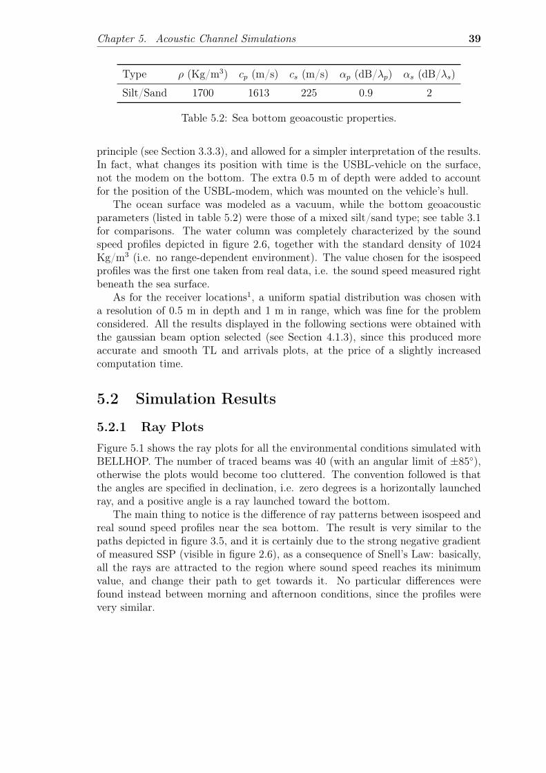
Chapter 5. Acoustic Channel Simulations 39
Type ρ (Kg/m3) cp (m/s) cs (m/s) αp (dB/λp) αs (dB/λs)
Silt/Sand 1700 1613 225 0.9 2
Table 5.2: Sea bottom geoacoustic properties.
principle (see Section 3.3.3), and allowed for a simpler interpretation of the results.In fact, what changes its position with time is the USBL-vehicle on the surface,not the modem on the bottom. The extra 0.5 m of depth were added to accountfor the position of the USBL-modem, which was mounted on the vehicle’s hull.
The ocean surface was modeled as a vacuum, while the bottom geoacousticparameters (listed in table 5.2) were those of a mixed silt/sand type; see table 3.1for comparisons. The water column was completely characterized by the soundspeed profiles depicted in figure 2.6, together with the standard density of 1024Kg/m3 (i.e. no range-dependent environment). The value chosen for the isospeedprofiles was the first one taken from real data, i.e. the sound speed measured rightbeneath the sea surface.
As for the receiver locations1, a uniform spatial distribution was chosen witha resolution of 0.5 m in depth and 1 m in range, which was fine for the problemconsidered. All the results displayed in the following sections were obtained withthe gaussian beam option selected (see Section 4.1.3), since this produced moreaccurate and smooth TL and arrivals plots, at the price of a slightly increasedcomputation time.
5.2 Simulation Results
5.2.1 Ray Plots
Figure 5.1 shows the ray plots for all the environmental conditions simulated withBELLHOP. The number of traced beams was 40 (with an angular limit of ±85◦),otherwise the plots would become too cluttered. The convention followed is thatthe angles are specified in declination, i.e. zero degrees is a horizontally launchedray, and a positive angle is a ray launched toward the bottom.
The main thing to notice is the difference of ray patterns between isospeed andreal sound speed profiles near the sea bottom. The result is very similar to thepaths depicted in figure 3.5, and it is certainly due to the strong negative gradientof measured SSP (visible in figure 2.6), as a consequence of Snell’s Law: basically,all the rays are attracted to the region where sound speed reaches its minimumvalue, and change their path to get towards it. No particular differences werefound instead between morning and afternoon conditions, since the profiles werevery similar.
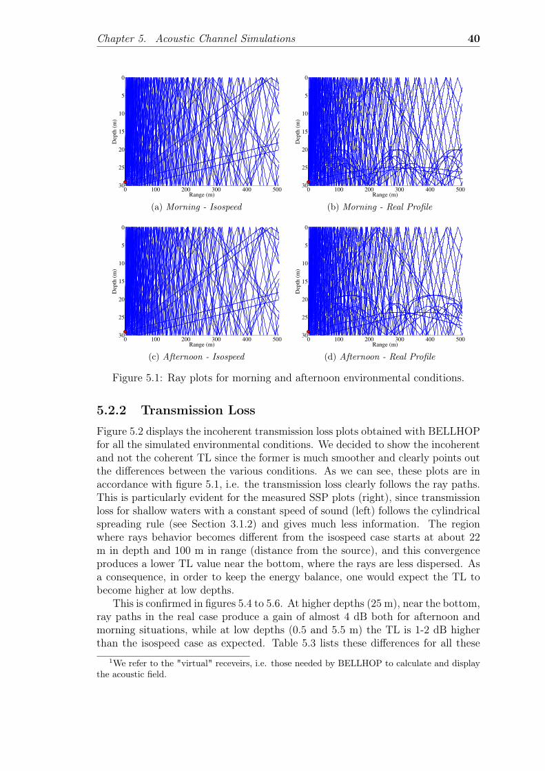
Chapter 5. Acoustic Channel Simulations 40
0 100 200 300 400 500
0
5
10
15
20
25
30
Range (m)
Dep
th (
m)
(a) Morning - Isospeed
0 100 200 300 400 500
0
5
10
15
20
25
30
Range (m)
Dep
th (
m)
(b) Morning - Real Profile
0 100 200 300 400 500
0
5
10
15
20
25
30
Range (m)
Dep
th (
m)
(c) Afternoon - Isospeed
0 100 200 300 400 500
0
5
10
15
20
25
30
Range (m)
Dep
th (
m)
(d) Afternoon - Real Profile
Figure 5.1: Ray plots for morning and afternoon environmental conditions.
5.2.2 Transmission Loss
Figure 5.2 displays the incoherent transmission loss plots obtained with BELLHOPfor all the simulated environmental conditions. We decided to show the incoherentand not the coherent TL since the former is much smoother and clearly points outthe differences between the various conditions. As we can see, these plots are inaccordance with figure 5.1, i.e. the transmission loss clearly follows the ray paths.This is particularly evident for the measured SSP plots (right), since transmissionloss for shallow waters with a constant speed of sound (left) follows the cylindricalspreading rule (see Section 3.1.2) and gives much less information. The regionwhere rays behavior becomes different from the isospeed case starts at about 22m in depth and 100 m in range (distance from the source), and this convergenceproduces a lower TL value near the bottom, where the rays are less dispersed. Asa consequence, in order to keep the energy balance, one would expect the TL tobecome higher at low depths.
This is confirmed in figures 5.4 to 5.6. At higher depths (25 m), near the bottom,ray paths in the real case produce a gain of almost 4 dB both for afternoon andmorning situations, while at low depths (0.5 and 5.5 m) the TL is 1-2 dB higherthan the isospeed case as expected. Table 5.3 lists these differences for all these
1We refer to the "virtual" receveirs, i.e. those needed by BELLHOP to calculate and displaythe acoustic field.

Chapter 5. Acoustic Channel Simulations 41
(a) Morning - Isospeed (b) Morning - Real Profile
(c) Afternoon - Isospeed (d) Afternoon - Real Profile
Figure 5.2: Incoherent TL plots for morning and afternoon environmental condi-tions.
cases: positive values show a higher TL for the real case, while negative ones alower TL (i.e. lower signal attenuation). We chose these values for the receiverranges (horizontal distances from the source) since they were the typical ranges ofoperation of the Typhoon vehicle during the CommsNet13 experiment.
Finally, no significant variations were found between morning and afternoonenvironmental conditions for real SSP simulations, see figure 5.3.
5.2.3 Arrivals
A very interesting and useful feature of BELLHOP is the creation of a file thatcontains all the arrivals (i.e. rays, parametrized by complex amplitude and phase)from the source for each specified receiver in the environment, together with theirdelay time. This is equivalent to construct the transfer function of the acousticchannel, and allows to better analyze signal transmission from source to receiver(which is what we did in Chapter 6).
To better capture and interpret the importance of these arrivals, we examineonce again three different receiver positions, in range: 200 m, 300 m and 400m. Receivers depths were 0.5 m for morning and 5.5 m for afternoon (where theTyphoon always stayed under the sea surface).
Figures 5.7 to 5.9 show the arrivals sequences as stem plots for morning ex-perimental conditions, comparing isospeed and real sound speed profile. Since ray

Chapter 5. Acoustic Channel Simulations 42
Receiver Environmental Receiver RangeDepth Conditions 200 m 300 m 400 m
0.5 m Morning 1.17 2.08 2.79Afternoon 0.97 1.68 2.32
5.5 m Morning 1.08 1.67 2.16Afternoon 0.99 1.48 1.93
25 m Morning -3.71 -3.84 -3.89Afternoon -2.91 -3.87 -4.07
Table 5.3: Incoherent TL difference from ideal to real case.
0 100 200 300 400 500
25
30
35
40
45
50
55
Range (m)
TL
(d
B)
Morning
Afternoon
(a) Depth 0.5 m
0 100 200 300 400 500
10
15
20
25
30
35
40
45
50
55
Range (m)
TL
(d
B)
Morning
Afternoon
(b) Depth 25 m
Figure 5.3: Morning and afternoon incoherent TL slices for real sound speed profile.
amplitude is a complex number (to account for phase changes and caustics), thequantity on the y-axis is its modulus. As one would expect, replicas of source signalincrease with range, due to reflections and multipath effects; the same happens forthe arrival times (greater distance to cover) and amplitude values, which decreasedue to geometrical spreading (at least). Another thing to point out is the highernumber of arrivals when the sound speed profile is the real one, which means thatsignal transmission encounters much more interference in this case.
Figures 5.10 to 5.12 do the same for afternoon simulations, and the same ex-act considerations can be made. It is worth noticing that, probably due to thehigher receiver’s depth, the arrivals number is higher too (with respect to morningconditions).
As previously stated, the importance of these data lies in the fact that theycan be convolved with the signal coming from source in order to obtain the signalthat reaches the receiver; this allows for an in-depth analysis of the transmissionconditions of the acoustic channel, which is the subject of the following chapter ofthis document.

Chapter 5. Acoustic Channel Simulations 43
0 100 200 300 400 500
25
30
35
40
45
50
55
Range (m)
TL
(d
B)
Isospeed
Real Profile
(a) Morning
0 100 200 300 400 500
25
30
35
40
45
50
55
Range (m)
TL
(d
B)
Isospeed
Real Profile
(b) Afternoon
Figure 5.4: Incoherent TL slice for isospeed and real profile simulations, receiverdepth 0.5 m.
0 100 200 300 400 500
25
30
35
40
45
50
55
Range (m)
TL
(d
B)
Isospeed
Real Profile
(a) Morning
0 100 200 300 400 500
25
30
35
40
45
50
55
Range (m)
TL
(d
B)
Isospeed
Real Profile
(b) Afternoon
Figure 5.5: Incoherent TL slice for isospeed and real profile simulations, receiverdepth 5.5 m.
0 100 200 300 400 500
10
15
20
25
30
35
40
45
50
55
Range (m)
TL
(d
B)
Isospeed
Real Profile
(a) Morning
0 100 200 300 400 500
10
15
20
25
30
35
40
45
50
55
Range (m)
TL
(d
B)
Isospeed
Real Profile
(b) Afternoon
Figure 5.6: Incoherent TL slice for isospeed and real profile simulations, receiverdepth 25 m.

Chapter 5. Acoustic Channel Simulations 44
0.12 0.14 0.16 0.18 0.2 0.220
0.5
1
1.5
2
2.5
3
3.5
4
4.5x 10
−3
Time (s)
Am
pli
tud
e
(a) Isospeed
0.12 0.14 0.16 0.18 0.2 0.220
0.5
1
1.5
2
2.5
3
3.5x 10
−3
Time (s)
Am
pli
tud
e
(b) Real Profile
Figure 5.7: Arrivals for receiver range 200 m, morning conditions.
0.18 0.2 0.22 0.24 0.26 0.280
0.5
1
1.5
2
2.5x 10
−3
Time (s)
Am
pli
tud
e
(a) Isospeed
0.18 0.2 0.22 0.24 0.26 0.280
0.2
0.4
0.6
0.8
1
1.2
1.4
1.6
1.8x 10
−3
Time (s)
Am
pli
tud
e
(b) Real Profile
Figure 5.8: Arrivals for receiver range 300 m, morning conditions.
0.26 0.27 0.28 0.29 0.3 0.31 0.320
0.2
0.4
0.6
0.8
1
1.2
1.4
1.6
1.8x 10
−3
Time (s)
Am
pli
tud
e
(a) Isospeed
0.26 0.27 0.28 0.29 0.3 0.31 0.320
0.2
0.4
0.6
0.8
1
1.2x 10
−3
Time (s)
Am
pli
tud
e
(b) Real Profile
Figure 5.9: Arrivals for receiver range 400 m, morning conditions.

Chapter 5. Acoustic Channel Simulations 45
0.12 0.14 0.16 0.18 0.2 0.22 0.240
0.5
1
1.5
2
2.5
3
3.5
4
4.5x 10
−3
Time (s)
Am
pli
tud
e
(a) Isospeed
0.12 0.14 0.16 0.18 0.2 0.22 0.240
0.5
1
1.5
2
2.5
3
3.5
4x 10
−3
Time (s)
Am
pli
tud
e
(b) Real Profile
Figure 5.10: Arrivals for receiver range 200 m, afternoon conditions.
0.18 0.2 0.22 0.24 0.26 0.280
0.5
1
1.5
2
2.5
3x 10
−3
Time (s)
Am
pli
tud
e
(a) Isospeed
0.18 0.2 0.22 0.24 0.26 0.280
0.5
1
1.5
2x 10
−3
Time (s)
Am
pli
tud
e
(b) Real Profile
Figure 5.11: Arrivals for receiver range 300 m, afternoon conditions.
0.26 0.27 0.28 0.29 0.3 0.31 0.320
0.2
0.4
0.6
0.8
1
1.2
1.4
1.6
1.8x 10
−3
Time (s)
Am
pli
tud
e
(a) Isospeed
0.26 0.27 0.28 0.29 0.3 0.31 0.320
0.2
0.4
0.6
0.8
1
1.2
1.4x 10
−3
Time (s)
Am
pli
tud
e
(b) Real Profile
Figure 5.12: Arrivals for receiver range 400 m, afternoon conditions.

Chapter 6
Transmission Quality Analysis
In Chapter 5, BELLHOP was used to completely characterize the underwateracoustic channel from CommsNet13 measured sound speed profiles, both for morn-ing and afternoon environmental conditions. The next step is to use the obtaineddata to analyze the transmission quality from source (the acoustic modem) to re-ceiver (the USBL-vehicle), which can be subjected to interference and multipatheffects, in order to explain possible communication failures and therefore to bet-ter design the geometry of communication for future experiments. This chapterdescribes and discusses in detail all the results obtained with this analysis.
The starting point were the arrivals files generated with BELLHOP for eachsimulation; as we previously stated, these files contain the amplitude-delay pairs ofthe propagated rays for each receiver, which can be used to construct the impulseresponse of the channel. Therefore, they played a central role in the received signalscalculation and in the following developments.
Section 6.2 contains the transmission quality analysis using the classical cross-correlation approach. We performed a simple cross-correlation calculation betweensource signal (input) and received signal (output) in order to test the correctnessof the transmission. If the signal is transmitted through the channel withoutinterference, we would see a delayed peak in the cross-correlation function, withthe delay due to the distance between source and receiver. If we set an appropriatethreshold, the receiver can correctly detect the signal reception when the peak isabove this value.
Section 6.3 describes the transmission quality analysis using source signal re-construction in the case of fixed geometry of communication (no source-receiverrelative motion). Assuming that the receiver knows the basic waveform the sourceimplements to send signals with, it can use this information together with the re-ceived signal in order to perform a reconstruction of the real (unknown) sourcesignal in two steps: first, estimate the impulse response of the system (the acousticchannel), then deconvolute the received signal through this impulse response toobtain an estimate of the source signal. The cross-correlation analysis betweenthis estimated source signal and an exact replica of the basic source signal canyield much better results for signal detection.
Section 6.4 repeats the steps described in the previous section for the case ofvariable geometry of communication (there is a source-receiver relative motion),which was the real situation encountered during the CommsNet13 experiment. If
46

Chapter 6. Transmission Quality Analysis 47
S
R1
2
3
Figure 6.1: A simple example of a source-receiver configuration in a waveguide.
0 0.5 1 1.5 2 2.5 3−1
0
1Source Signal
0 0.5 1 1.5 2 2.5 3−0.5
0
0.5
1Impulse Response
Time [s]
Figure 6.2: Source signal and channel impulse response example.
this happens, the received waveform is influenced by the Doppler shifts determinedby the relative motion, which must be taken into account when signal detection isperformed.
The mathematical tools used to produce all the results presented in this chap-ter are described in the appendices. Received signal calculation (Appendix A)makes use of the Hilbert transform of the source signal, since rays are described bycomplex pressure to accounts for phase changes and caustics. Then Appendices Band C explain the methods, correlation analysis and deconvolution via regularizedleast squares, which were used to eliminate multipath effects and to test whetherthe receiver can obtain an accurate reconstruction of the real transmitted signal.
6.1 Source Signal and Cross-CorrelationFigure 6.1 illustrates a simple example of a waveguide where a source (S) emitsthree acoustic rays which arrive at a receiver (R) in three different ways: the firstone directly, the second one reflected by the sea surface and the third one reflectedby the sea bottom. Each of these rays (arrivals) constitute a replica of the originalsignal, and their summation at the receiver creates interference.
To better illustrate this fact we can see figures 6.2 and 6.3. We suppose that

Chapter 6. Transmission Quality Analysis 48
0 0.5 1 1.5 2 2.5 3
−1
0
1
x 10−3 Received Signal
0 0.5 1 1.5 2 2.5 3−1
0
1Input−Output Cross−Correlation
Time [s]
Figure 6.3: Received signal and cross-correlation for the previous example.
−0.01 0 0.01 0.02 0.03 0.04 0.05 0.06 0.07 0.08−1.5
−1
−0.5
0
0.5
1
1.5
Time [s]
Am
pli
tude
0.0162 0.0162 0.0162−1
0
1
Figure 6.4: Source signal (sweeping sinusoid), with an enlargement.
the impulse response of the channel is known and has the structure representedin figure 6.2. If we make the convolution between this impulse response and thesource signal, we get the received signal shown in figure 6.3; in order to see whathappened to the original one, we can calculate the cross-correlation between inputand output using equation (B.4), and the correlation function clearly highlightsthe presence of the three signal replicas over time.
The same analysis was done for signal transmission between source and receiverduring CommsNet13 sea trials. Now, the impulse response is available thanks tothe arrivals files produced by BELLHOP. The waveform used as the source signalwas a chirp (sweeping sinusoid), which is implemented on the EvoLogics acousticmodem mounted on the USBL-vehicle. The lowest frequency was 18 kHz, while thehighest was 34 kHz. The chirp duration was 40 ms, while the total time windowof observation was 80 ms. The signal is shown in figure 6.4, with an enlargementto point out its structure. It is well-known that chirps properties produce an auto-correlation equal to a sinc function with the peak perfectly centered in the originof the time axis, as we can see from figure 6.5.
As for the received signal visualization, the time scale was chosen as the reducedtime (see [14, pagg. 615-616]), which represents a relative time that takes into

Chapter 6. Transmission Quality Analysis 49
−0.08 −0.06 −0.04 −0.02 0 0.02 0.04 0.06 0.08−1000
−500
0
500
1000
1500
Delay τ [s]
Input Auto−Correlation
Figure 6.5: Source signal auto-correlation function.
account the distance between source and receiver. It is usually calculated as:
tred = t− r
cred, (6.1)
where t is the absolute time, r is the receiver range and cred is the reduced speed ofsound, which should always exceed the fastest possible arrival. For our purposes,we chose cred = 1700m/s.
We previously stated that typical horizontal vehicle distances from the source(ranges) were 200 m, 300 m and 400 m. Hereinafter, for the sake of space, allthe results will be shown only for range equal to 200 m (both during morning andafternoon), since results for the other two cases were very similar. We also needto point out that this whole analysis was made in the case of exact knowledge ofall signals (deterministic case), without the influence of noise or other sources oferror (stochastic case).
6.2 Signal Detection with Classic CorrelationFigure 6.6 display the received signals calculated for morning and afternoon envi-ronmental conditions when the receiver range is equal to 200 m. Figure 6.7 doesthe same for their cross-correlation functions with the original source signal.
It becomes immediately clear that the original signal reaches the receiver heav-ily distorted and attenuated due to the interference and multipath reflections ofthe acoustic channel. Cross-correlation shapes clearly reflect the arrivals depictedin figure 5.7 (for morning) and figure 5.10 (for afternoon), and the attenuationbecomes greater as range increases.
It is impossible for the receiver to correctly detect the signal, since a) there is atremendous loss between auto-correlation and cross-correlation values (the formerreaches a peak of almost 1500, the latter between 2 and 6), and b) the ratiosbetween the first and the second peak in cross-correlation functions are too small,which means that, even if we set an appropriate threshold on the cross-correlation

Chapter 6. Transmission Quality Analysis 50
0 0.01 0.02 0.03 0.04 0.05 0.06 0.07 0.08−1.5
−1.0
−0.5
0.0
0.5
1.0
1.5Received Signal
Reduced Time [s]
×10−2
(a) Morning
0 0.01 0.02 0.03 0.04 0.05 0.06 0.07 0.08−1.5
−1.0
−0.5
0.0
0.5
1.0
1.5Received Signal
Reduced Time [s]
×10−2
(b) Afternoon
Figure 6.6: Received signals for morning and afternoon conditions, range 200 m.
0 0.01 0.02 0.03 0.04 0.05 0.06 0.07 0.08−6
−4
−2
0
2
4
6Input−Output Cross−Correlation
Time [s]
(a) Morning
0 0.01 0.02 0.03 0.04 0.05 0.06 0.07 0.08−5
0
5Input−Output Cross−Correlation
Time [s]
(b) Afternoon
Figure 6.7: Cross-correlation functions for morning and afternoon conditions, range200 m.
for signal detection, the receiver becomes too sensible to fluctuations of the signal(noise, outliers, . . . ).
6.3 Signal Detection with Source Estimation
6.3.1 Impulse Response Estimation
The first step in source signal estimation was to use the received signal and an exactreplica of the basic source waveform to obtain an estimate of the impulse responseof the channel. As previously mentioned, the procedure (correlation analysis) isdescribed in Appendix B and the results are shown in figure 6.8. The number Mof samples used during this process was exactly the half of the original signals.
If we make a comparison with the cross-correlation functions shown in figure 6.7we see that the impulse response estimate is very reliable (they both give informa-tion on signal replicas over time) and similar to the original one; the only differenceis the absence of the last part due to the reduced number of samples, but this values

Chapter 6. Transmission Quality Analysis 51
0 0.01 0.02 0.03 0.04 0.05 0.06 0.07 0.08−4
−3
−2
−1
0
1
2
3
4x 10
−3 Impulse Response Estimate
Time [s]
Am
pli
tude
(a) Morning
0 0.01 0.02 0.03 0.04 0.05 0.06 0.07 0.08−4
−3
−2
−1
0
1
2
3
4x 10
−3 Impulse Response Estimate
Time [s]
Am
pli
tude
(b) Afternoon
Figure 6.8: Impulse response estimates for morning and afternoon conditions, range200 m.
are very small and have non influence on signal estimation.
6.3.2 Source Signal Estimation
Then, the estimated impulse response and the received signal can be used to per-form a deconvolution to obtain the source signal. The receiver can perform a cross-correlation between this one and the true waveform in order to ensure the correctsignal detection. Since the values of all the vectors are very small the problemis bad-conditioned, so we were forced to use a modified deconvolution algorithmwhich introduces a regularization parameter λ (as described in Appendix C); theresults of the deconvolution are therefore influenced by the values of this scalarparameter.
Figures 6.9 and 6.10 show the results of this process for two values of λ. In thefirst case, the regularization parameter is high (compared to the order of magnitudeof signal values), and this produces an estimate of the source signal which is toosimilar to the received signal1. Even though the cross-correlation between themhas a single peak centered at the origin of the time axis (which is what we want),the value of this peak is still too small because of received signal attenuation dueto channel effects.
The second case is the opposite: the regularization parameter value is nowvery small, and this does not solve the deconvolution numerical problems, thatare clearly visible in the left part of figure 6.10. Cross-correlation has now abigger peak at the beginning, but the presence of oscillations in the right part isundesired, since we want this function to be the most similar possible to a standardchirp auto-correlation function (figure 6.5).
6.3.3 Regularization Parameter Sensitivity
We then performed a sensitivity analysis of the estimate based on this parame-ter. We calculated the source signal estimate for every value of λ on an equally
1This means that the λI term in equation (C.4) dominates.
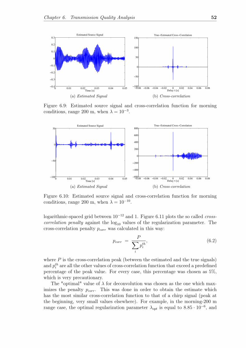
Chapter 6. Transmission Quality Analysis 52
0 0.01 0.02 0.03 0.04 0.05−0.4
−0.3
−0.2
−0.1
0
0.1
0.2
0.3Estimated Source Signal
Time [s]
(a) Estimated Signal
−0.08 −0.06 −0.04 −0.02 0 0.02 0.04 0.06 0.08−100
−50
0
50
100
150True−Estimated Cross−Correlation
Delay τ [s]
(b) Cross-correlation
Figure 6.9: Estimated source signal and cross-correlation function for morningconditions, range 200 m, when λ = 10−3.
0 0.01 0.02 0.03 0.04 0.05−100
−50
0
50Estimated Source Signal
Time [s]
(a) Estimated Signal
−0.08 −0.06 −0.04 −0.02 0 0.02 0.04 0.06 0.08−600
−400
−200
0
200
400
600
800True−Estimated Cross−Correlation
Delay τ [s]
(b) Cross-correlation
Figure 6.10: Estimated source signal and cross-correlation function for morningconditions, range 200 m, when λ = 10−10.
logarithmic-spaced grid between 10−12 and 1. Figure 6.11 plots the so called cross-correlation penalty against the log10 values of the regularization parameter. Thecross-correlation penalty pcorr was calculated in this way:
pcorr =P∑i
pthi, (6.2)
where P is the cross-correlation peak (between the estimated and the true signals)and pthi are all the other values of cross-correlation function that exceed a predefinedpercentage of the peak value. For every case, this percentage was chosen as 5%,which is very precautionary.
The "optimal" value of λ for deconvolution was chosen as the one which max-imizes the penalty pcorr. This was done in order to obtain the estimate whichhas the most similar cross-correlation function to that of a chirp signal (peak atthe beginning, very small values elsewhere). For example, in the morning-200 mrange case, the optimal regularization parameter λopt is equal to 8.85 · 10−6, and

Chapter 6. Transmission Quality Analysis 53
Environment Range Peak λopt
Morning200 m 555.61 8.85 · 10−6
300 m 586.47 2.07 · 10−6
400 m 638.94 1.13 · 10−7
Afternoon200 m 676.54 2.63 · 10−8
300 m 671.96 6.16 · 10−9
400 m 576.17 2.07 · 10−6
Table 6.1: Cross-correlation peaks and λopt for conditions of interest.
−12 −10 −8 −6 −4 −2 00
0.2
0.4
0.6
0.8
1
1.2
1.4Sensitivity to Regularization
Log10
λ
Cro
ss−
Corr
elat
ion P
enal
ty
Figure 6.11: Sensitivity analysis to regularization parameter for morning condi-tions, range 200 m.
it produces a cross-correlation peak of 555.61; the estimated source signal and thecross-correlation function are visible in figure 6.12.
Table 6.1 lists the results of this procedure for every condition of interest. Theconclusions are quite straightforward: if the receiver implements even a simplereconstruction procedure as the one described in this section, it can get rid ofthe interference and multipath effects of the acoustic channel, obtain a good es-timate of the true source signal and, setting up an appropriate threshold for thecross-correlation peak value, correctly detect its transmission. In practice, acousticmodems and transponders implement even more refined reception algorithms.
6.4 Signal Detection with Doppler ShiftThe results showed in the previous sections are valid for the case of stationarysource-receiver configuration. Since the receiver (the USBL-vehicle) was movingduring the experiment, the frequency shifts due to Doppler effects must be takeninto account during received signal calculations, as explained in the last part ofAppendix A.
The magnitude of the Doppler effect is proportional to the ratio a = v/c of the

Chapter 6. Transmission Quality Analysis 54
0 0.01 0.02 0.03 0.04 0.05−0.8
−0.6
−0.4
−0.2
0
0.2
0.4
0.6
0.8Estimated Source Signal
Time [s]
(a) Estimated Signal
−0.08 −0.06 −0.04 −0.02 0 0.02 0.04 0.06 0.08−400
−200
0
200
400
600True−Estimated Cross−Correlation
Delay τ [s]
(b) Cross-correlation
Figure 6.12: Estimated source signal and cross-correlation function for morningconditions, range 200 m, when λ = λopt.
0 0.01 0.02 0.03 0.04 0.05 0.06 0.07 0.08−0.015
−0.01
−0.005
0
0.005
0.01
0.015Received Signal (with and without Doppler effects)
Reduced Time [s]
Am
pli
tude
No Doppler
Dopplerized
(a) Morning
0 0.01 0.02 0.03 0.04 0.05 0.06 0.07 0.08−0.015
−0.01
−0.005
0
0.005
0.01
0.015Received Signal (with and without Doppler effects)
Reduced Time [s]
Am
pli
tude
No Doppler
Dopplerized
(b) Afternoon
Figure 6.13: Received signals comparison with and without Doppler effects at range200 m, receiver speed 1 m/s.
relative transmitter-receiver velocity to the speed of sound. Because the speed ofsound is very low compared to the speed of electromagnetic waves, motion-inducedDoppler distortion of an acoustic signal can be extreme. For comparison, in thecase of a mobile radio system, at 160 km/h we have a = 1.5 · 10−7. This valueis low enough that Doppler spreading can be neglected. Instead, a stationaryacoustic system may experience unintentional motion at 0.5 m/s (1 knot), whichwould account for a = 3 · 10−4. For an AUV moving at several meters per second(submarines can move at much greater velocities), factor a will be on the order of10−3, a value that cannot be ignored [26].
Figure 6.13 shows the comparison between the received signals calculated withand without Doppler effects, when the horizontal speed of the vehicle is equal to1 m/s (i.e. 2 knots)2. As wee can see, the only substantial difference from thestationary case is a slightly higher attenuation of the signal, while its shape (theresulting envelope produced by the convolution with the arrivals) remains the same.At much higher speeds, for example 10 m/s (see figure 6.14), there is also a time
2The typical vehicles speeds during CommnsNet13 trials were 0.5, 1 and 1.5 knots.

Chapter 6. Transmission Quality Analysis 55
0 0.01 0.02 0.03 0.04 0.05 0.06 0.07 0.08−0.015
−0.01
−0.005
0
0.005
0.01
0.015Received Signal (with and without Doppler effects)
Reduced Time [s]
Am
pli
tud
e
No Doppler
Dopplerized
Figure 6.14: Received signals comparison with and without Doppler effects formorning conditions at range 200 m, receiver speed 10 m/s.
shift, which is significant especially at the higher frequencies of the signal (rightpart), but once again the signal shape remains the same.
We used the dopplerized signals in the reconstruction procedure described inSection 6.3, and results were exactly the same (we do not report them for thesake of brevity). This means that the Doppler shifts do not influence the impulseresponse of the acoustic channel, and become significant only at very high relativespeeds between source and receiver, which fall out the range of interest for ouranalysis.

Conclusions
Starting with real data of sound speed profiles, and using the ray tracing numer-ical simulator BELLHOP with the appropriate settings, the acoustic environmen-tal conditions of the La Spezia Gulf during CommsNet13 trials were completelycharacterized. The differences from a standard isospeed profile, typical of shallowwaters during winter, were examined; we saw that the strong negative gradient ofmeasured SSPs near the bottom produces a convergence of the ray paths, whichtranslates in a lower TL at high depths and, to maintain the energy balance, ahigher TL at low depths (the ones the USBL-vehicle was operating at).
Then, with the contribution of amplitude-delay arrivals files generated fromBELLHOP simulations, an extensive analysis was done of the transmission qualitybetween source (the USBL-vehicle) and receiver (the moored modems) in theseconditions. Using a standard chirp waveform as the source signal, we realized thatthe interference and multipath effects produced by the acoustic channel greatlyworsen the signal transmission, and the signal reaches the receiver distorted andpoorly correlated with the original one. Therefore, assuming that the receiverknows the basic waveform the source uses to communicate with, it could followa mathematical procedure to reconstruct the source signal starting from the re-ceived one, in two steps: impulse response estimation with correlation analysis andsource signal estimation using regularized least squares deconvolution. The resultsobtained clearly showed that with this procedure the receiver can get rid of all theinterference and, after obtaining an estimate of the source signal which is very closeto the real one, greatly improve the transmitted signal reception. Both the casesof stationary and non-stationary source-receiver configurations were analyzed.
The contents of this thesis were elaborated in order to try to explain the ir-regular acoustic position fixes encountered in the localization of the USBL-vehicleduring CommsNet13 sea trials. Since we showed that the acoustic channel influ-ences can be eliminated with an appropriate reception algorithm, they could onlybe explained in two ways:
• The acoustic modems were working at the limit of their detection threshold,which means that the little changes in TL between isospeed and measuredprofiles (table 5.3) become significant.
• Fluctuations in sound speed values and/or other physical parameters canhave some influence and therefore they must be taken into account.
More data must be collected and further analyses and simulations must be donein order to more accurately explain these phenomena.
56

Appendix A
Received Signal Calculation
This section is based on [14, pagg. 617-619]. Received signal calculation using theformulation of ray theory in the time domain has a particularly simple form. Wedenote the source signal with s(t). The easiest way of obtaining the desired resultis to start with the pressure contribution of a single eigenray (see Section 4.1):
p(s) = A(s)eiωτ(s), (A.1)
where A(s) is the amplitude and τ(s) is the phase delay along the ray path s:
τ(s) =
∫ s
0
1
c(s′)ds′. (A.2)
We assume that the loss, and therefore the amplitude term A(s), is independent offrequency. A time domain solution can be directly obtained by Fourier synthesisas:
p(s, t) =1
2π
∫ +∞
−∞S(ω)p(s, ω)e−iωt dω, (A.3)
where S(ω) represents the spectrum of the source. Substituting the ray represen-tation for p(s, ω), we obtain:
p(s, t) = A(s)1
2π
∫ +∞
−∞S(ω)e−iω[t−τ(s)] dω, (A.4)
that is:
p[s, t+ τ(s)
]= A(s)
1
2π
∫ +∞
−∞S(ω)e−iωt dω. (A.5)
We can recognize the integral as simply the inverse Fourier transform so that:
p[s, t+ τ(s)
]= A(t)S(t), (A.6)
or, equivalently:p(s, t) = A(s)S
[t− τ(s)
]. (A.7)
Thus, the received signal is simply a scaled and delayed replica of the source signal.The scaling factor, i.e. the change in amplitude of the source signal, is determinedby the change in the cross-sectional area of a ray tube.
57

Appendix A. Received Signal Calculation 58
A key assumption in the above description is that the amplitude A(s) is purelyreal. As discussed before, boundary reflections typically cause phase changes. Inaddition, Gaussian beam tracing creates more general phase changes. In short,A(s) = Ar(s) + iAi(s) is generally a complex number. We require A(s, ω) =A∗(s,−ω), where ω is the angular frequency, to ensure the resulting waveform ispurely real. In the simplest case, we can assume A(s, ω) = Ar(s) + isgn(ω)Ai(s),with the frequency dependence entirely embedded in the sign function. Substitut-ing this in equation (A.3) we obtain:
p(s, t) = Ar(s)1
2π
∫ +∞
−∞S(ω)e−iω[t−τ(s)] dω +
Ai(s)1
2π
∫ +∞
−∞isgn(ω)S(ω)e−iω[t−τ(s)] dω.
(A.8)
Recall that the Hilbert transform S(t) is a 90◦ phase change of an arbitrary wave-form S(t), and is therefore defined by [27]:
S(t) =1
2π
∫ +∞
−∞−isgn(ω)S(ω) dω. (A.9)
Since 1/(πt) is the inverse transform of −isgn(ω), we may also write the Hilberttransform as the time domain convolution of the source waveform with (πt):
S(t) =1
π
∫ +∞
−∞
S(t)
t− τdt. (A.10)
The frequency-domain representation is usually more convenient. In either case:
p(s, t) = Ar(s)S[t− τ(s)
]− Ai(s)S
[t− τ(s)
]. (A.11)
Equation (A.11) is the complete expression for the received signal and it impliesthat the received waveform is a weighted sum of the original one and its Hilberttransform, with the weighting determined by the strengths of the real and imagi-nary parts of the amplitudes. Note that the Hilbert transform produces an acausalsignal, reflecting another artifact of ray theory (see Section 4.1.3). This equationis the key result showing the form of a single echo or path, including phase changesdue to propagation delay, boundary reflections, and caustic phase shifts.
This solution is valid for stationary problems, i.e. for environment and source-receiver configurations fixed throughout the duration of the propagation. For realsonar environments, this is not always a valid assumption, especially for the caseof moving source and/or receiver. It is well known that a moving source/receiverin free space results in a frequency Doppler shift which is described by the simplerelations obtained from a Galilean transformation. In a waveguide or stratified en-vironment, source-receiver motion results in a more complicated Doppler structurebecause of multipath phenomena.
If the environment is time-varying, the arrival amplitudes and delays in equa-tion (A.1) change continuously in time. Therefore, new values of A(s) and τ(s) arerequired at each time step of the signal transmission. In theory, at each time step,

Appendix A. Received Signal Calculation 59
a new set of arrival amplitudes and delays could be computed with an entirelynew ray trace from the source to the exact receiver location at that particular timestep. However, this would be computationally expensive and mostly unnecessarysince the changes (in amplitude and delay) are likely to be very small between timesteps.
Several solutions are available in the literature to account for Doppler shifts;for the standard practical case of moving source/receiver configuration, the Vir-TEX algorithm is one of the simplest and most efficient (see [28, 29] for completedetails), and allows the calculation of the received signal without the need of atime-dependent ray tracer.

Appendix B
Correlation Analysis
This section is based on [30]. Correlation analysis allows for the estimation of theimpulse response of a linear systems when input-output cross-correlation and inputauto-correlation are available. Consider a discrete LTI system with disturbancev(t):
y(t) =+∞∑k=0
h(k)u(t− k) + v(t). (B.1)
Assume u and v have zero mean and E[u(t)v(s)
]= 0 ∀t, s. The correlation
function is given by:
Ryu(τ) = E[y(t+ τ)u(t)
]=
+∞∑k=0
h(k)Ruu(τ − k). (B.2)
If u(t) is white noise (Ruu(τ) = 0, τ 6= 0), equation (B.2) is simplified to:
Ryu(k) = h(k)Ruu(0). (B.3)
Cross-correlation and auto-correlation functions can be estimated from input andoutput signals using a finite number of samples N :
Ryu(τ) =1
N
N−τ∑t=1
y(t+ τ)u(t) τ = 0, 1, 2, . . .
Ruu(τ) =1
N
N−τ∑t=1
u(t+ τ)u(t) τ = 0, 1, 2, . . .
(B.4)
Using equations (B.4), equation (B.3) can be solved to find the impulse responseestimate h(k).
When u(t) is not exactly white, there are two solutions:
• Apply a so called whitening filter : filter both inputs and outputs in order tomake the input as white as possible;
• Truncate the impulse response at a certain order.
60
Appendix B. Correlation Analysis 61
The second solution assumes that:
h(k) = 0 k > M. (B.5)
This is a finite impulse response (FIR) filter, or truncated weighting function, andM is the order of the filter.
The correlation equation becomes therefore:
Ryu(τ) =M∑k=0
h(k)Ruu(τ − k). (B.6)
Writing out this equation for τ = 0, 1, . . . ,M gives the linear system:Ryu(0)
Ryu(1)...
Ryu(M)
=
Ru(0) Ru(1) . . . Ru(M)
Ru(−1) Ru(0) . . . Ru(M − 1)...
... . . . ...Ru(−M) Ru(−M + 1) . . . Ru(0)
h(0)
h(1)...
h(M)
(B.7)
which can be solved to obtain h(k). The system matrix is the convolution matrix(or Toeplitz matrix ) of the discrete system, and it is symmetric due to the symmetryof the auto-correlation function for real signals.
Appendix C
Deconvolution via Least Squares
The deconvolution problem is the process of extracting the input signal in a linearsystem when the output signal is available (and preferably the impulse responsetoo). Several solutions can be found in the literature; for our purposes, a deconvo-lution that makes use of Tikhonov regularization (also known as ridge regression)was chosen.
Deconvolution can always be written as a standard linear system of equations:
y = Hu, (C.1)
where H is the deconvolution matrix. The standard approach for its solution(known as ordinary least squares, or simply least squares) seeks to minimize thesum of squared residuals:
u = minu‖y −Hu‖2 , (C.2)
where ‖·‖ is the Euclidean norm. Since matrix H could be near to singularity, andthe solution therefore too sensible to numerical approximations, a regularizationterm can be included in this minimization. That is:
u = minu‖y −Hu‖2 + ‖Γu‖2 , (C.3)
for some suitably chosen Tikhonov matrix Γ. A closed form solution is availableas:
u =(HTH + ΓTΓ
)−1HTy. (C.4)
The effects of regularization may be varied via the scale of matrix Γ. For Γ = 0this reduces to the classical, unregularized, least squares solution provided that(HTH
)−1 exists. In many cases, Tikhonov matrix is chosen as a multiple of theidentity matrix Γ = λI, giving preference to solution with smaller norms.
62

Appendix D
AcTUP Quick Start Guide
This section is based on [25]. A brief guide for setting up a simulation with theBELLHOP version included in the front-end will be given. With this toolbox,instead of writing and editing each time the .env file (Section 4.2.1) which definesthe simulation, the user can exploit the simple GUI-structure of the software whichprovide intelligent guesses and selection guidelines for code-specific parameters.
At the end of installation instructions, after running AcTUP the user will see amenu-driven system; the following basic steps must be followed in order to configureand launch the simulation:
• Configure Environment & Propagation ModelsThe most important section. Launches another menu which allows the userto define all the necessary environmental and simulation parameters. EditEnvironment launches an interface to edit the model environment. The usercan specify each layer’s structure (water column, sediment, vacuum) and geo-physical parameters. Sound speed profiles can be imported from a .txt filearranged in depth-value pairs. Edit Code-Independent Propagation Parame-ters is the section that contains the basic parameters (frequency, source andreceiver depths,. . . ) defining the propagation scenario. These parametersare common to each propagation code. Edit Code-Dependent PropagationParameters is the section where additional information must be provided forsome codes, reflecting their numerical features. In the case of BELLHOP,these are the simulation type (ray tracing, transmission loss, arrivals), thebeam type (geometric, gaussian), the beam number, and other minor ones.All the specified settings can be saved as a .mat file with the command SaveRun Definition for future use.
• Select Active CodeSince AcTUP is a GUI-wrapper for each model included in the AcousticToolbox, the user can the select them with this command. The name of thecurrent code always appears on the right.
• Run Current Model for ACTIVE Propagation CodeRuns the environment/propagation model currently in memory using theselected propagation code. The simulation time is displayed in the Matlabworkspace.
63

Appendix D. AcTUP Quick Start Guide 64
• Plotting Tools
Simulations results (rays, transmission loss fields and slices, amplitude-delayarrivals,. . . ) can be displayed using the commands available in this section,which are largely self-explanatory.
We must remember that BELLHOP is essentially a high-frequency code, and al-though its useful frequency range extends lower than standard ray trace programs,it should be used with extreme caution in situations where the water depth or thesize of any significant feature in the sound speed profile is less than 20 wavelengths(see Section 4.1). In these cases, the use of another model (KRAKEN, SCOOTER)should be preferred.

Bibliography
[1] L. Paull et al. “AUV navigation and localization: A review”. In: OceanicEngineering, IEEE Journal of 39.1 (2014), pp. 131–149.
[2] L. Stutters et al. “Navigation technologies for autonomous underwater vehi-cles”. In: Systems, Man, and Cybernetics, Part C: Applications and Reviews,IEEE Transactions on 38.4 (2008), pp. 581–589.
[3] J. C. Kinsey, R. M. Eustice, and L. L. Whitcomb. “A survey of underwatervehicle navigation: Recent advances and new challenges”. In: IFAC Confer-ence of Manoeuvering and Control of Marine Craft. 2006.
[4] Woods Hole Oceanograpic Institution. url: http://www.whoi.edu/.
[5] Teledyne Technologies. url: http://www.teledyne.com/.
[6] EvoLogics. url: http://www.evologics.de/.
[7] B. Allotta et al. “Typhoon at CommsNet 2013: experimental experience onAUV navigation and localization”. In: Advances in Robotics and Control,IFAC (2015, in press).
[8] A. Caiti et al. “Thesaurus: AUV teams for archaeological search. Field resultson acoustic communication and localization with the Typhoon”. In: Controland Automation (MED), 2014 22nd Mediterranean Conference of. IEEE.2014, pp. 857–863.
[9] B. Allotta et al. “Typhoon at CommsNet 2013: experimental experience onAUV navigation and localization”. In: Proc. IFAC World Congress. 2014.
[10] A. Caiti et al. “Experimental results with a mixed USBL/LBL system forAUV navigation”. In: Underwater Communications and Networking (UComms),2014. IEEE. 2014, pp. 1–4.
[11] A. Caiti et al. “Fusing acoustic ranges and inertial measurements in AUVnavigation: The Typhoon AUV at CommsNet13 sea trial”. In: OCEANS2014-TAIPEI. IEEE. 2014, pp. 1–5.
[12] F. Di Corato et al. “Toward underwater acoustic-based simultaneous localiza-tion and mapping. Experimental results with the Typhoon AUV at Comm-sNet13 sea trial”. In: Oceans-St. John’s, 2014. IEEE. 2014, pp. 1–7.
[13] D. R. Topham and R. G. Perkin. “CTD sensor characteristics and theirmatching for salinity calculations”. In: Oceanic Engineering, IEEE Journalof 13.3 (1988), pp. 107–117.
[14] F. B. Jensen et al. Computational Ocean Acoustics. Springer, 2011.
65

Bibliography 66
[15] J. M. Hovem. Marine Acoustics: The Physics of Sound in Underwater Envi-ronments. Peninsula Publishing, 2012.
[16] L. M. Brekhovskikh and Y. P. Lysanov. Fundamentals of Ocean Acoustics.Springer, 2003.
[17] R. J. Urick. Principles of Underwater Sound. McGraw-Hill, 1983.
[18] E. Lewis. “The practical salinity scale 1978 and its antecedents”. In: OceanicEngineering, IEEE Journal of 5.1 (1980), pp. 3–8.
[19] V. A. Del Grosso. “New equation for the speed of sound in natural waters(with comparisons to other equations)”. In: The Journal of the AcousticalSociety of America 56.4 (1974), pp. 1084–1091.
[20] F. E. Hale. “Long-range sound propagation in the deep ocean”. In: The Jour-nal of the Acoustical Society of America 33.4 (1961), pp. 456–464.
[21] M. B. Porter. The BELLHOP Manual and User’s Guide: Preliminary Draft.Heat, Light, and Sound Research, Inc., La Jolla, CA, USA, Tech. Rep. 2011.
[22] A. J. Duncan and A. L. Maggi. “A consistent, user friendly interface forrunning a variety of underwater acoustic propagation codes”. In: Proceedingsof ACOUSTICS. 2006, pp. 471–477.
[23] Ocean Acoustics Library. url: http://oalib.hlsresearch.com/.
[24] O. Rodriguez. General description of the BELLHOP ray tracing program.Universidade do Algarve. 2008.
[25] A. J. Duncan and A. L. Maggi. AcTUP v2.2L Acoustic Toolbox User-Interface& Post-Processor–Installation & User Guide. Curtin University of Technol-ogy, Perth. 2006.
[26] M. Stojanovic and J. Preisig. “Underwater acoustic communication channels:Propagation models and statistical characterization”. In: CommunicationsMagazine, IEEE 47.1 (2009), pp. 84–89.
[27] N. E. Huang and S. S. Shen. Hilbert-Huang transform and its applications.Vol. 5. World Scientific, 2005.
[28] M. Siderius and M. B. Porter. “Modeling broadband ocean acoustic trans-missions with time-varying sea surfaces”. In: The Journal of the AcousticalSociety of America 124.1 (2008), pp. 137–150.
[29] J. C. Peterson and M. B. Porter. “Ray/beam tracing for modeling the effectsof ocean and platform dynamics”. In: Oceanic Engineering, IEEE Journal of38.4 (2013), pp. 655–665.
[30] L. Ljung. System Identification: Theory for the User. Prentice Hall, 1999.