optimization of the anaerobic digestion process by substrate pre
TRANSCRIPT
NEER ENGI
OPTIMIZATION OF THE ANAEROBIC DIGESTION PROCESS BY SUBSTRATE PRE-TREATMENT AND THE APPLICATION OF NIRS Biological and Chemical Engineering Technical Report BCE-TR-1

DATA SHEET Title: Optimization of the anaerobic digestion process by substrate pre-treatment and the application of NIRS Subtitle: Biological and Chemical Engineering Series title and no.: Technical report BCE-TR-1 Author: Chitra Sangaraju Raju Department of Engineering, Biological and Chemical Engineering, Aarhus University Internet version: The report is available in electronic format (pdf) at the Department of Engineering website http://www.eng.au.dk. Publisher: Aarhus University© URL: http://www.eng.au.dk Year of publication: 2012 Pages: 96 Editing completed: May 2012 Abstract: Biogas production is a complex process depending on many factors and is an area that is being researched intensively. This thesis is based on studies that were aimed at optimizing the biogas production process by: • Reducing the time taken to assess the biochemical methane poten-tials (BMP) of substrates (specifically meadow grasses) by rapid analyti-cal methods such as near infra-red spectroscopy (NIRS), in-vitro organic matter digestibility assay and the neutral detergent fibre assay • Applying NIRS as a monitoring tool to assess the concentrations of ammonia (which is inhibitory to the process) in the contents of anaero-bic digesters. • Improving the BMP of materials such as cattle manure and dewatered pig manure and chicken manure by thermal pre-treatment at various temperatures between 100°C and 225°C Results show that the NIRS method can be used to discriminate be-tween meadow grasses with high or low BMP. In detecting the ammo-nia content, NIRS was shown to have the potential to be a process mon-itoring tool. Thermal pre-treatment proved to be most effective on de-watered pig manure which showed improvements at lower pre-treatment temperatures. Cattle manure required pre-treatment temper-atures higher than 175°C to show improvement. Chicken manure did not show any improvements but instead showed a decrease in BMP at 225°C. Keywords: Alternative energy sources, Bioenergy, Biogas, Biomass, En-ergy production, Environmental engineering, NIR, Manure, Pretreatment technologies, Sensor technologies, Spectroscopy, Sustainable technolo-gies Supervisors: Henrik Bjarne Møller & Alastair James Ward Please cite as: C. Raju, 2012. Optimization of the anaerobic digestion process by substrate pre-treatment and the application of NIRS. De-partment of Engineering, Aarhus University. Denmark. 96 pp. - Technical report BCE -TR-1 Cover photo: Carolyn Schaffer ISSN: 2245-5817 Reproduction permitted provided the source is explicitly acknowledged
.

OPTIMIZATION OF THE ANAEROBIC DIGESTION PROCESS BY SUBSTRATE
PRE-TREATMENT AND THE APPLICATION OF NIRS
Chitra Sangaraju Raju
Aarhus University, Department of Engineering
Abstract Biogas production is a complex process depending on many factors and is an area that is being researched intensively. This thesis is based on studies that were aimed at optimizing the biogas production process by:
• Reducing the time taken to assess the biochemical methane potentials (BMP) of substrates (specifically meadow grasses) by rapid analytical methods such as near infra-red spectroscopy (NIRS), in-vitro organic matter digestibility assay and the neutral detergent fibre assay
• Applying NIRS as a monitoring tool to assess the concentrations of ammonia (which is inhibitory to the process) in the contents of anaerobic digesters.
• Improving the BMP of materials such as cattle manure and dewatered pig manure and chicken manure by thermal pre-treatment at various temperatures between 100°C and 225°C
Results show that the NIRS method can be used to discriminate between meadow grasses with high or low BMP. In detecting the ammonia content, NIRS was shown to have the potential to be a process monitoring tool. Thermal pre-treatment proved to be most effective on dewatered pig manure which showed improvements at lower pre-treatment temperatures. Cattle manure required pre-treatment temperatures higher than 175°C to show improvement. Chicken manure did not show any improvements but instead showed a decrease in BMP at 225°C.
1
Preface
This thesis is submitted as a requirement for the completion of my PhD degree. The
research work was carried out during the period of December 2008 to February 2012 at
what is now the Department of Engineering, Foulum campus, Aarhus University. My work
was supervised by Henrik Bjarne Møller as my main supervisor and by Alastair James
Ward as my co-supervisor.
The thesis consists of a general introduction, a chapter on near infrared spectroscopy and a
chapter on pre-treatment of substrates. Each of the last two chapters ends with a summary
of the results that are derived from the papers that were written based on the experiments
that were performed as part of the PhD study. Two of the papers have been published
while the third paper has been accepted for publication.
The titles of the papers are:
1. Comparison of near infra-red spectroscopy, neutral detergent fibre assay and in-
vitro organic matter digestibility assay for rapid determination of the biochemical
methane potential of meadow grasses
2. NIR monitoring of ammonia in anaerobic digesters using diffuse reflectance probe
3. Effects of high temperature isochoric pre-treatment on the methane yields of cattle,
pig and chicken manure
This thesis would not have been possible without the support and encouragement of both
my supervisors Henrik and Alastair. I would like to thank my mum, my family, my friends
and my colleagues for their love and support. Special thanks to Heidi and Britt for all the
help in the lab.
Foulum, February 2012,
Chitra Sangaraju Raju

2
Acknowledgements
I would like to thank all the people who made a difference in my life, to those who held me afloat
when I needed it the most, to the people who had more faith in me than myself, to those who
shaped me and are shaping me and to those who made this PhD possible. This thesis is for you.

3
Summary
Biogas production is fast gaining importance as a source of renewable energy apart from
being a waste management solution. There are several areas in the biogas production
process that need optimization and research, and this PhD study focused on the following
areas.
1. The application of near infrared spectroscopy (NIRS) in the anaerobic digestion
process
2. Pre-treatment of substrates to improve their methane yields.
The amount of methane that can be obtained from a particular substrate is usually
measured by the biochemical methane potential assay (BMP) which requires at least 30
days. NIRS along with two forage analysis techniques, the in-vitro organic matter
digestibility assay (IVOMD) and the neutral detergent fibre assay (NDF) were tested as
methods that could be used to predict the BMP of meadow grasses in much less time. The
NIRS method was most successful as a rapid and indirect method of predicting the BMP
when compared to the other two methods. The NIRS method required the use of partial
least squares regression, a multivariate data analysis approach, to build models that
related the spectral data from the NIRS to the BMPs of the meadow grasses. The model
based on NIRS had an R2 value of 0.69 and a residual prediction deviation (RPD) of 1.75,
which makes it a moderately useful model that can discriminate between high and low
values of BMP for meadow grasses.
Another study where NIRS was applied to the anaerobic digestion process was to monitor
the total ammonia nitrogen contents (TAN) of an anaerobic digester. Ammonia is a known
inhibitor and beyond certain levels, can seriously affect the anaerobic digestion process. It
is currently measured mainly by chemical analysis. The use of NIRS to measure the
ammonia contents would reduce the time and the chemicals required for laboratory
analysis and make real time monitoring possible. A diffuse reflectance probe attached to an
NIR spectrometer was used to measure the TAN contents in the digestates of anaerobic
digesters that used cattle manure as substrate. Partial least squares regression and interval
partial least squares methods were used to build models of spectral data predicting the
TAN concentrations. An R2 of 0.91 and an RPD of 3.4 was obtained implying that the probe
could be used for monitoring and screening purposes.
The second focus of this PhD study was to use pre-treatment methods to improve the BMP
of substrates. Three types of manure, cattle manure, dewatered pig manure and chicken
manure were subjected to thermal pre-treatment and the changes in their BMP were
studied. The manures were pre-treated in a high temperature and pressure reactor for 15
minutes, at six temperatures between 100°C and 225°C with 25°C intervals to study the
effect on their methane yield. After 27 days of anaerobic digestion, the dewatered pig
manure showed improvements at much lower pre-treatment temperatures when compared

4
to the other two manures. All temperatures above 125°C improved the BMP of the pig
manure with a maximum 29 % increase in yield at 200°C. Cattle manure showed a
significant improvement in its BMP at temperatures above 175°C with the best result of a
21 % increase at 200°C. The BMP in chicken manure was reduced by 18 % at 225°C, but at
lower pre-treatment temperatures there were no significant changes.
5
Summary in Danish
Biogas som en kilde til produktion af vedvarende energi vinder hurtigt frem da det udover
at producere energi også giver en række miljøfordele og er en miljøvenlig metode til
affaldshåndtering. Der er imidlertid flere områder, der kræver optimering før teknologien
er fuldt udviklet og denne ph.d undersøgelse har fokus på en række områder der kan
optimere teknologien herunder:
Anvendelse af nær-infrarød spektroskopi (NIRS) til process optimering og biogas udbytte
måling
Forbehandling af substrater for at forbedre methan udbyttet.
Mængden af methan, der kan opnås fra et substrat måles normalt ved biokemiske metan
assays (BMP), der tager mindst 30 dage. NIRS sammen med to foder analyseteknikker (in
vitro-organisk stof (IVOS) og neutral detergent fiber (NDF) er blevet afprøvet som metode
til at forudsige BMP af vedvarende græs. NIRS metoden var den bedste og hurtigste
metode til forudsigelse af BMP i forhold til de to andre fremgangsmåder. NIRS metoden
kræver anvendelse af mindste kvadraters regression og en multivariat dataanalyse tilgang
til lave modeller, der vedrører de spektrale data fra NIRS til BMP af engen græss. Modellen
baseret på NIRS havde en R2 værdi på 0,69 og afvigelse (RPD) på 1,75, svarende til en
anvednelig model som kan skelne mellem høje og lave værdier af BMP i eng græsser.
I en anden undersøgelse blev NIRS anvendt til at overvåge det samlede ammoniak indhold
(TAN) i en anaerob udrådnings processen. Ammoniak er en kendt inhibitor, og kan
påvirke den anaerobe nedbrydningsproces negativt hvis niveauet kommer over bestemte
niveauer. I øjebliket måles ammoniak ved kemisk analyse der er tids- og
omkostningskrævende. Anvendelsen af NIRS til at måle ammoniak indholdet vil reducere
den tid og de kemikalier, der kræves til laboratorieanalyse og gøre real time overvågning
muligt. En diffus reflektans probe forbundet til en NIR spektrometer blev anvendt til at
måle TAN indholdet i biogas reaktorer med kvæggødning substrat. En R2 på 0,91 og en
RPD på 3,4 blev opnået som indebærer, at proben er anvendelig til overvågnings- og
screening formål.
Det andet fokusområde forbehandling metoder til forbedring af BMP værdien for
forskellige substrater. Tre typer af husdyrgødning, kvæggylle, afvandet svinegylle og
hønsegødning blev udsat for termisk forbehandling og ændringer i BMP blev undersøgt.
Husdyrgødningen blev forbehandlet i en høj temperatur og tryk reaktor i 15 minutter ved
seks temperaturer fra 100°C - 225°C med 25°C intervaller og efterfølgende blev virkningen
på deres methan udbytte undersøgt. Efter 27 dages anaerob udrådning var der positiv
effekt på afvandet svinegødning ved lavere forbehandlings temperaturer sammenlignet
med de to andre gødningstyper. Alle temperaturer over 125 ° C forbedrede BMP af
svinegylle med en maksimal stigning på 29% i udbytte ved 200°C. Kvæggylle viste en
signifikant forbedring i BMP ved temperaturer over 175°C med det bedste resultat på 21%

6
forbedring ved 200°C. BMP i hønsegødning blev reduceret med 18% ved 225 ° C, men ved
lavere temperaturer var der ingen signifikante effekter.
7
Glossary
AD Anaerobic digestion
BMP Biochemical methane potential
CSTR Continuous stirred tank reactor
DM Dry matter
EMSC Extended multiplicative scatter correction
FT-NIR Fourier transform near infrared spectroscopy
HRT Hydraulic retention time
InAs Indium Arsenide
InGaAs Indium Gallium Arsenide
IVOMD In-vitro organic matter digestibility test
LFA Long chain fatty acids
LV Latent variables
NDF Neutral detergent fibre
NIR Near infrared
NIRS Near infrared spectroscopy
MSC Multiplicative scatter correction
OLR Organic loading rate
PCA Principal component analysis
PC Principal component
PC/MR Principal component regression
PLS Partial least squares
PLSR Partial least squares regression
R2 Coefficient of determination
RMSECV Root mean square error of cross validation
RMSEP Root mean square error of prediction

8
RPD Residual prediction deviation/ ratio of standard deviation to standard error of
performance
RPM Rotations per minute
SD Standard deviation
SNV Standard normal variate
TAN Total ammonia nitrogen
VFA Volatile fatty acids
VS Volatile solids

9
Table of Contents
Summary ..................................................................................................................... 3
Summary in Danish ..................................................................................................... 5
Glossary ....................................................................................................................... 7
Chapter 1 - Introduction ..................................................................................................... 11
1.1 Biogas as a renewable energy source ..................................................................... 11
1.2 The anaerobic process .......................................................................................... 13
Hydrolysis: ........................................................................................................ 13
Acidogenesis and Acetogenesis: ........................................................................ 13
Methanogenesis: ............................................................................................... 14
1.3 Factors affecting biogas production: .................................................................... 16
1.4 Substrates for biogas production: ........................................................................ 18
1.5 Objectives of the PhD study: ................................................................................ 19
1.6 Overview of the thesis structure: ......................................................................... 20
1.7 List of papers: ...................................................................................................... 20
Chapter 2 - NIRS in Anaerobic digestion: .......................................................................... 21
2.1 Introduction: ........................................................................................................ 21
2.2 Application of NIR in the anaerobic digestion process: ....................................... 23
2.3 Equipment and materials: ................................................................................... 24
2.4 Multi-variate data analysis software: ................................................................... 24
2.5 Data analysis: ...................................................................................................... 25
Principal component analysis (PCA): ................................................................ 25
Data pre-processing: ......................................................................................... 25
Partial least squares (PLS) regression and interval PLS (iPLS): ........................ 26
2.6 Summary of results:............................................................................................. 26
Chapter 3 – Pre-treatment of substrates ............................................................................28
3.1 Necessity of pre-treatment ...................................................................................28
3.2 Lignocellulosic components................................................................................. 29
Lignin................................................................................................................ 29
Cellulose ........................................................................................................... 29
Hemicellulose ................................................................................................... 29
3.3 Various methods of pre-treatment .......................................................................30

10
Mechanical ........................................................................................................30
Thermal ............................................................................................................30
Chemical ...........................................................................................................30
Biological .......................................................................................................... 31
3.4 Pre-treatment method used in this PhD study: .................................................... 31
Equipment ........................................................................................................ 32
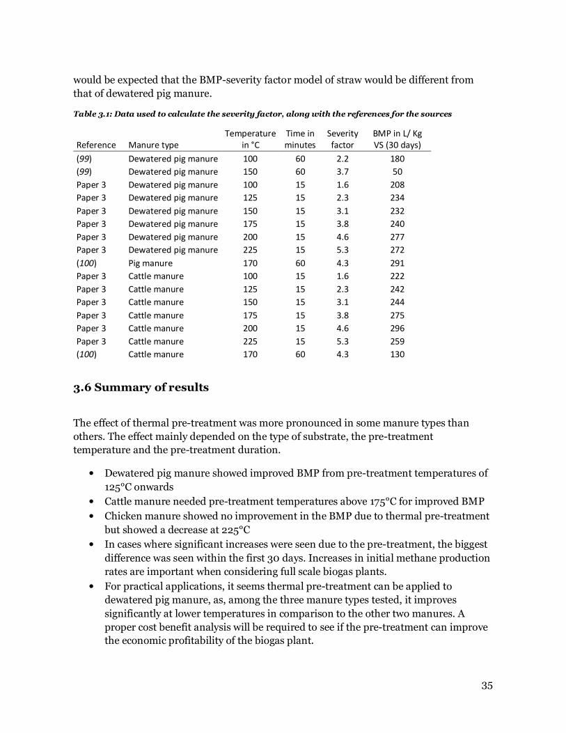
3.5 Severity factor ...................................................................................................... 33
3.6 Summary of results .............................................................................................. 35
Appendix ........................................................................................................................... 37
Paper 1 ....................................................................................................................... 38
Comparison of near infra-red spectroscopy, neutral detergent fibre assay and in-
vitro organic matter digestibility assay for rapid determination of the
biochemical methane potential of meadow grasses.
Paper 2 ...................................................................................................................... 49
NIR monitoring of ammonia in anaerobic digesters using diffuse reflectance
probe.
Paper 3 ...................................................................................................................... 61
Effects of high temperature isochoric pre-treatment on the methane yields of
cattle, pig and chicken manure.
Report ....................................................................................................................... 87
Optimizing the sample presentation method - (unpublished data).
11
Chapter 1 - Introduction
1.1 Biogas as a renewable energy source
Anaerobic digestion (AD) is a biological process where organic matter is degraded into its
most reduced form (methane) and its most oxidized form (carbon dioxide) without
external electron acceptors such as oxygen, nitrates or sulphates (1, 2). The process occurs
in nature and is one of the natural degradation pathways for organic matter. The main
gaseous products of anaerobic digestion are methane and carbon dioxide, and minor
quantities (< 1%) of hydrogen sulphide, nitrogen oxides, ammonia and other volatile
compounds (1). Although there has been evidence of the use of biogas for heating in the
10th century BC, the first anaerobic digesters appeared in the mid 19th century. The initial
use of digesters was mainly for sewage treatment. It was then extended to handle animal
manure, municipal solid wastes and wastes from industries such as food, pharmaceutical
and chemical industries. The energy crisis in the 1970’s led to a significant growth in
research in this area as there was an impetus to reduce the dependency on fossil fuels (3,
4). More recently, AD is being considered as a potential renewable energy source and not
just as a waste treatment solution.
AD is a viable solution to some of the problems that the world is facing today and to those
that are expected to arise in the near future. The world population is increasing and is
expected to reach nine billion by the year 2040 and as a consequence the energy demand is
expected to rise by 30% (5). Currently about 81% of the worlds energy demand is met by
fossil fuels (6). The amount of fossil fuels available is limited and the use of fossil fuels is
one of the main causes for anthropogenic greenhouse gas emissions. Greenhouse gases, as
their name suggests, trap heat on to the earth’s surface increasing the average global
temperature, leading to serious environmental impacts such as the melting of the polar ice-
caps, severe weather fluctuations, increased frequency of droughts and acidification of
oceans to name a few (7). Energy production using fossil fuels is responsible for about 57%
of the total greenhouse gas emissions (8). Biogas is a carbon dioxide (CO2) neutral source
of energy, in other words it uses the carbon that is already available in the existing carbon
cycle and does not add to it and is hence a good substitute for fossil fuels.
Population growth will also lead to an increase in the amount of waste generated. Biogas
produced from AD of wastes such as municipal solid wastes, agricultural residues and
wastewater sludge, generates energy while reducing the volume of the waste. It also
harnesses the methane emissions associated with the wastes; for example landfill
emissions and emissions from manure storage. Methane is a potent greenhouse gas. It has
a high greenhouse gas potential and is 21 times more effective (over a 100 year period) at
trapping heat than carbon dioxide (9). 50% of the methane emissions on earth are by
human activities such as livestock production, manure management, coal mining, landfills
and rice production among others (10). AD of wastes that might have caused emissions in

12
landfills and from manure storage will reduce the amount of methane emitted to the
atmosphere. In other words, the methane emissions from landfills and manure storage can
be reduced considerably by using their organic fractions to produce methane under
controlled conditions, and then collecting and utilizing the methane, effectively reducing
the impact.
Compared to other renewable energy sources AD has certain advantages and
disadvantages. Almost any organic matter can be degraded (to various extents depending
on the substrate properties) to produce biogas. It can thus utilize agricultural residues such
as crop residues and manure, and does not have to compete for land used for food
production. If energy crops are being used, biogas production uses the entire plant instead
of specific plant parts, like grain in the case of first generation bioethanol (11). The AD
process does not need pure microbial cultures (12) it has a multitude of microorganisms
working together and these microorganisms can be supplied as an initial inoculum or can
be found in the feedstock in manure substrates and will find a steady population if the
substrate input remains constant. As long as the substrate supply and the process is steady,
the production of biogas can be maintained at a steady rate, this is an advantage when
compared to renewable energy sources such as wind energy and solar energy that depend
on weather conditions. The digestate (the material remaining after AD) is nutrient rich; the
total nitrogen and phosphorous nutrient content remains the same in the digestate as in
the original biomass as the only significant elements removed are carbon, hydrogen and
oxygen in the form of biogas (13). Another advantage of the biogas process is that no
product separation is required; methane has very low solubility in water and readily
separates and collects in the headspace of the digester (12). Increase in bacterial biomass is
much lower in anaerobic digestion when compared to the amount of sludge produced by
aerobic or anoxic processes, as the amount of energy that the microbes gain in the
anaerobic process is much lower in comparison (2, 13).
However, a major issue with anaerobic systems is process instability, usually caused by
inhibition, feed overload, inadequate temperature control or washout of biomass (14, 15).
Some of the features that make AD an attractive option are also responsible for a lot of
issues that need attention. For example, it is an advantage to have multiple groups of
microbes working together, but a disturbance in the synergy between the groups could lead
to process failure. Currently, a lot of research is being focussed at making the process more
reliable and efficient.
The following sub-sections will give an outline of the basics behind the anaerobic process
followed by the factors that affect the biogas production and then a short paragraph on
substrates for the production of biogas, which all lead to the topics that were investigated
as part of this PhD study.
13
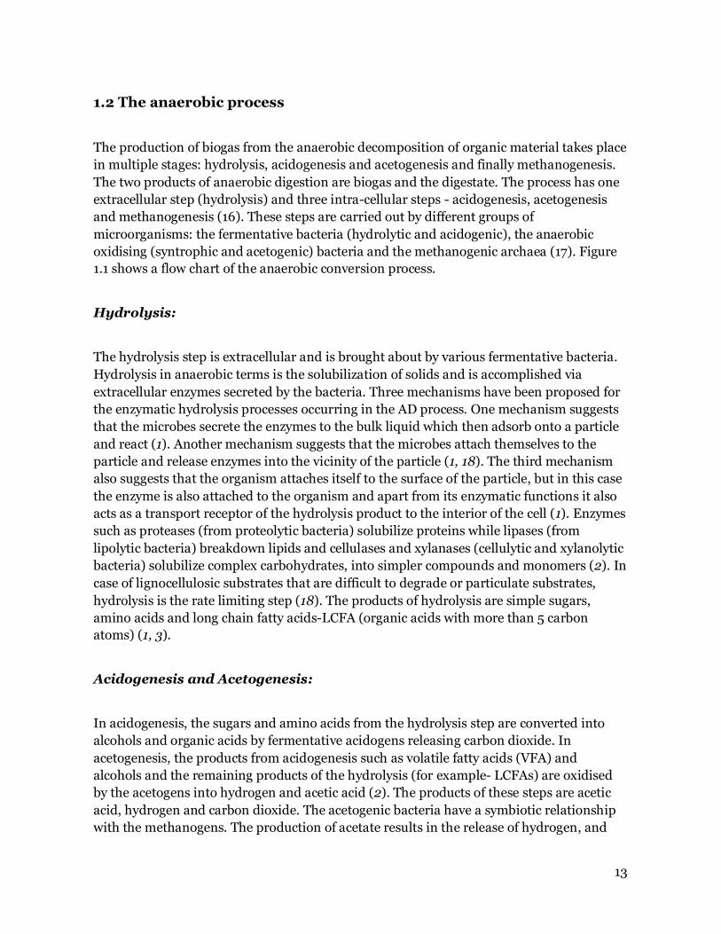
1.2 The anaerobic process
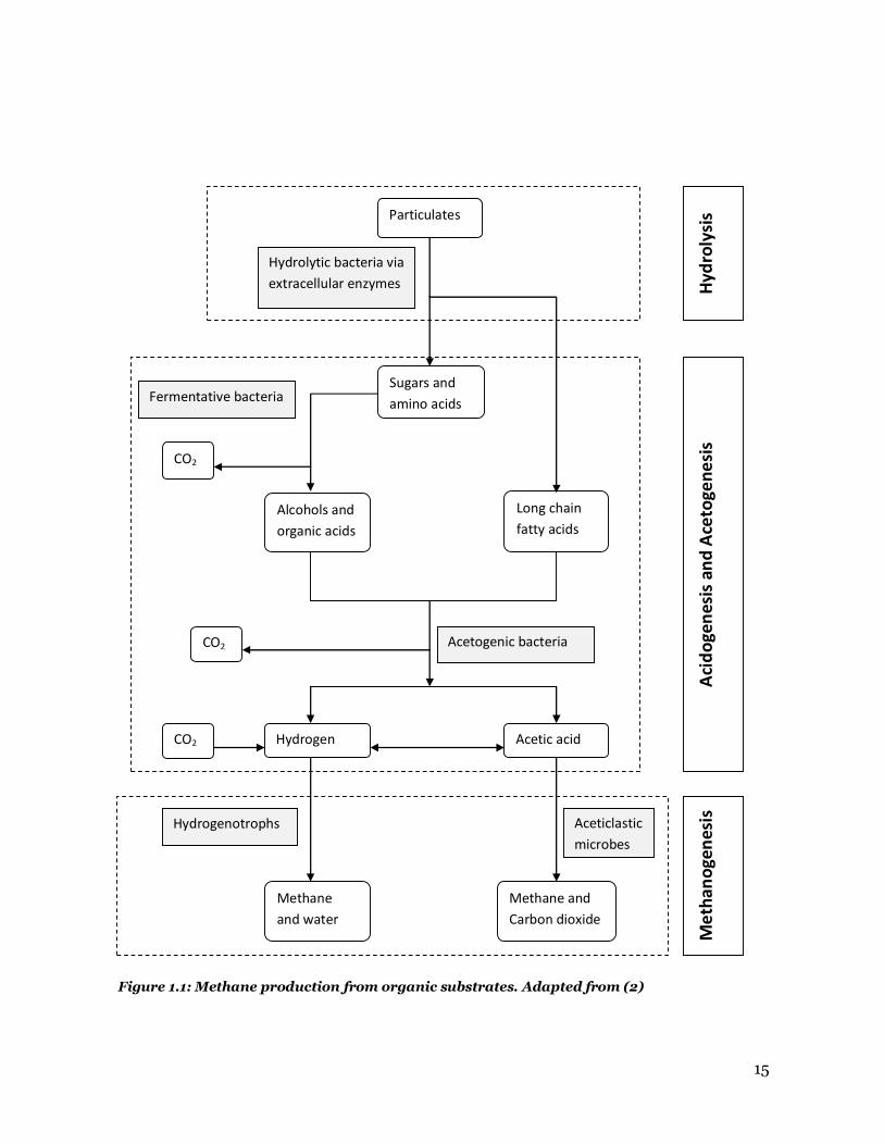
The production of biogas from the anaerobic decomposition of organic material takes place
in multiple stages: hydrolysis, acidogenesis and acetogenesis and finally methanogenesis.
The two products of anaerobic digestion are biogas and the digestate. The process has one
extracellular step (hydrolysis) and three intra-cellular steps - acidogenesis, acetogenesis
and methanogenesis (16). These steps are carried out by different groups of
microorganisms: the fermentative bacteria (hydrolytic and acidogenic), the anaerobic
oxidising (syntrophic and acetogenic) bacteria and the methanogenic archaea (17). Figure
1.1 shows a flow chart of the anaerobic conversion process.
Hydrolysis:
The hydrolysis step is extracellular and is brought about by various fermentative bacteria.
Hydrolysis in anaerobic terms is the solubilization of solids and is accomplished via
extracellular enzymes secreted by the bacteria. Three mechanisms have been proposed for
the enzymatic hydrolysis processes occurring in the AD process. One mechanism suggests
that the microbes secrete the enzymes to the bulk liquid which then adsorb onto a particle
and react (1). Another mechanism suggests that the microbes attach themselves to the
particle and release enzymes into the vicinity of the particle (1, 18). The third mechanism
also suggests that the organism attaches itself to the surface of the particle, but in this case
the enzyme is also attached to the organism and apart from its enzymatic functions it also
acts as a transport receptor of the hydrolysis product to the interior of the cell (1). Enzymes
such as proteases (from proteolytic bacteria) solubilize proteins while lipases (from
lipolytic bacteria) breakdown lipids and cellulases and xylanases (cellulytic and xylanolytic
bacteria) solubilize complex carbohydrates, into simpler compounds and monomers (2). In
case of lignocellulosic substrates that are difficult to degrade or particulate substrates,
hydrolysis is the rate limiting step (18). The products of hydrolysis are simple sugars,
amino acids and long chain fatty acids-LCFA (organic acids with more than 5 carbon
atoms) (1, 3).
Acidogenesis and Acetogenesis:
In acidogenesis, the sugars and amino acids from the hydrolysis step are converted into
alcohols and organic acids by fermentative acidogens releasing carbon dioxide. In
acetogenesis, the products from acidogenesis such as volatile fatty acids (VFA) and
alcohols and the remaining products of the hydrolysis (for example- LCFAs) are oxidised
by the acetogens into hydrogen and acetic acid (2). The products of these steps are acetic
acid, hydrogen and carbon dioxide. The acetogenic bacteria have a symbiotic relationship
with the methanogens. The production of acetate results in the release of hydrogen, and
14
acetogens which are obligate hydrogen producers cannot function at a hydrogen partial
pressure above 10-4 atmospheres (19). Methanogens utilize the hydrogen to produce
methane and keep the partial pressure of hydrogen low enough for the acetogens to
function. Two other processes can take place when two distinct groups of microbes, the
homoacetogens and the acetic acid oxidisers are present (20, 21). These two groups of
microbes cause the inter-conversion of acetate to hydrogen and carbon dioxide (syntrophic
acetate oxidation) and the conversion of hydrogen and carbon dioxide to acetate
(homoacetogenesis) (21).
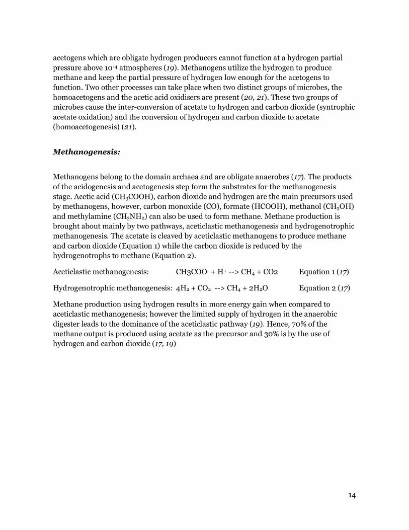
Methanogenesis:
Methanogens belong to the domain archaea and are obligate anaerobes (17). The products
of the acidogenesis and acetogenesis step form the substrates for the methanogenesis
stage. Acetic acid (CH3COOH), carbon dioxide and hydrogen are the main precursors used
by methanogens, however, carbon monoxide (CO), formate (HCOOH), methanol (CH3OH)
and methylamine (CH3NH2) can also be used to form methane. Methane production is
brought about mainly by two pathways, aceticlastic methanogenesis and hydrogenotrophic
methanogenesis. The acetate is cleaved by aceticlastic methanogens to produce methane
and carbon dioxide (Equation 1) while the carbon dioxide is reduced by the
hydrogenotrophs to methane (Equation 2).
Aceticlastic methanogenesis: CH3COO- + H+ --> CH4 + CO2 Equation 1 (17)
Hydrogenotrophic methanogenesis: 4H2 + CO2 --> CH4 + 2H2O Equation 2 (17)
Methane production using hydrogen results in more energy gain when compared to
aceticlastic methanogenesis; however the limited supply of hydrogen in the anaerobic
digester leads to the dominance of the aceticlastic pathway (19). Hence, 70% of the
methane output is produced using acetate as the precursor and 30% is by the use of
hydrogen and carbon dioxide (17, 19)
15
Figure 1.1: Methane production from organic substrates. Adapted from (2)
Particulates
Sugars and
amino acids
Long chain
fatty acids
Hydrogen Acetic acid
Alcohols and
organic acids
CO2
CO2
Methane
and water
Methane and
Carbon dioxide
Hydrolytic bacteria via
extracellular enzymes
Fermentative bacteria
Acetogenic bacteria
Hydrogenotrophs Aceticlastic
microbes
Hy
dro
lysi
s A
cid
og
en
esi
s a
nd
Ace
tog
en
esi
s M
eth
an
og
en
esi
s
CO2

16
1.3 Factors affecting biogas production:
From the previous section it can be seen that anaerobic digestion is a complex process and
requires the synergistic efforts of various microorganisms in various steps where the
products of one step are utilized in the next one finally culminating in the production of
biogas. A disturbance in one of the steps will therefore affect the entire process, and there
are numerous factors that affect the process.
Parameters such as organic loading rates, temperature, pH, concentrations of nutrients
and inhibitors such as ammonia and hydrogen sulphide are critical to the functioning of
the AD process. Table 1.1 shows some of the parametric levels that must be maintained in
digesters for optimal performance and the levels beyond which they are detrimental to the
AD process.
The effect of these parameters are different on different microbial groups as each microbial
group has different physiological and nutritional needs and different growth rates and it is
imbalances between them that causes process instability (22). An imbalance in the process
caused due to a disturbance in the hydrolysis stage will limit the activities in the
consequent stages reducing the biogas production (19). A disturbance in the last stage that
is the methanogenesis stage will bring about an accumulation of acids that have been
formed in the previous stages (19). Changes in the process such as reduced biogas
production, accumulation of VFAs, decrease in pH and alkalinity, increased concentrations
of carbon dioxide are indicators of process instability (19).
Table 1.1: Factors affecting anaerobic processes.
Parameter Optimal levels Detrimental levels
pH 6 to7 for methanogens and acetogens 6 for acidogens (4)
<6 and >8.5 (4)
Temperature 30°C to 35°C for mesophilic reactors (19) 50°C to 60°C for thermophilic reactors (19)
Fluctuation > ± 2°C/day to 3°C/day (19) Fluctuation > ± 1°C / day (15, 19)
Organic loading rate Depends on the composition of the substrate
> + 50% dissolved COD/day (15)
Free ammonia < 0.2 g N/L (22) 1.7 to 14 gN/L (22) (Depends on the degree of acclimatization)
Changes in pH and changes in gas production or in gas composition are usually slow and
while they can indicate gradual changes, they cannot be used to detect sudden changes in
the process (23). Process instabilities lead to an accumulation of VFA which should lead to
a corresponding drop in the pH. But in case of wastes that have a large buffer capacity;

17
manure for example, the pH change is noticeable only after the VFA concentration is very
high. Thus, although pH is an easy parameter to measure and can easily be applied to
online monitoring of reactors, it cannot be solely relied upon to monitor inhibition. On the
other hand, VFA, which by itself in high concentrations is inhibitory to methanogens, can
also be used as a process indicator (23). Some studies have suggested the use of individual
volatile fatty acids such as propionic acid, acetic acid, butyric acid, iso-butyric acid or iso-
valeric acid, as process indicators (24, 25). There is, however, no consensus on a general
level of VFA that is inhibitory as the level depends on various factors, but unexpected
increases in VFA could be seen as a sign of process imbalance that could possibly lead to
process failure if the anaerobic process does not adapt to the new levels (26, 27).
Among a number of compounds that are toxic to the anaerobic microbes, ammonia is the
most common inhibitor (4). However, ammonia concentrations below 200 mg/L are
favourable for anaerobic microbes as it is an essential nutrient (22). Ammonia is present in
the form of the ammonium ion (NH4+) and free ammonia (NH3), of which the free
ammonia (FA) is suspected to be the main cause for inhibition as it is membrane
permeable and can diffuse into the microbial cells (22). Of all the microbes that are part of
the anaerobic process, the methanogens are least tolerant to ammonia inhibition (22). The
ammonium ion and FA exist in equilibrium, and the equilibrium depends on the
temperature and pH. Increases in pH lead to an increase in concentration of FA (28).
Anaerobic digesters are operated typically at mesophilic (20°C to 45°C) or thermophilic
(45°C to 60°C) temperatures; those operated at temperatures below 20°C and are called
psychrophilic reactors (29). Higher operating temperatures usually result in higher
degradation rates and higher microbial growth rates, but also make the process more
unstable and susceptible to ammonia inhibition (1, 4, 28). The increase in the FA
concentration along with temperature makes thermophilic reactors more susceptible to
ammonia inhibition compared to mesophilic reactors.
The organic loading rate (OLR) is the substrate input rate per unit volume of the reactor in
terms of its organic content. The OLR is taken into consideration when deciding on the
hydraulic retention time (HRT) of a reactor (27). In other words, each reactor with a
particular HRT is designed to handle a certain organic load. Overloading will cause an
initial increase followed by a decrease in biogas production and the accumulation of VFAs
which if severe enough can inhibit the methanogens (27). Currently, feeding strategies in
full scale anaerobic digesters are volumetric or gravimetric and not based on the actual
quality of the input substrate (30). This is not an issue with farm based digesters which are
usually designed to handle waste from a particular farm. In case of reactors where the
substrates are mixtures of wastes or where complex substrates such as agricultural wastes
whose quality can vary are used, it is important to be able to assess the substrate quality in
terms of the amount of degradable solids and the amount of inhibitors if any. This is
mainly in order to optimize the substrate utilization and hence the biogas production.
18
1.4 Substrates for biogas production:
The substrate used to produce biogas in a digester is an important aspect that determines
the OLR, the amount of biogas and the methane fraction of the biogas produced (2). The
amount of biogas that can be produced from a particular substrate can be determined in
various ways. The biochemical methane potential (BMP) assay is the most common
experimental way to determine the amount and the rate of methane that can be produced
from a substrate (31). This method was proposed by Owen et. al. in 1979 and is a batch
process (32). A known amount of substrate is introduced into a flask containing a known
amount of inoculum(an active culture of anaerobic bacteria), and if necessary, a nutrient
solution (13). The flask is sealed and placed into an incubator maintained at a chosen
temperature and the biogas production is measured over a given time period or till the
biogas production is negligible over a long time period. The results are usually expressed in
unit volume of biogas or methane produced per unit weight of volatile solids that was
added as substrate. Although the results of a BMP batch test cannot be directly compared
to the outcome that can be expected in a full scale continuous reactor, the assay provides a
basis for comparison among different substrates. The disadvantage of the batch assay is
the time taken for the experiment. While 30 days is the recommended time period over
which the biogas production should be measured, some studies have used up to 100 days
to test the BMP of recalcitrant substrates (32, 33). Due to the long time period required to
assess the BMP of a material, in full scale operations, substrates are fed by weight or
volume based on previous experience, and not based on the actual substrate quality and
thus real-time adjustments of substrate input cannot be made (34). A reduction in the time
taken to assess the methane potential of substrates will enable real time assessment of
substrates in full scale biogas plants. Rapid assessment of the methane potential of feed-
stock that is to be purchased can be used to determine its monetary value.
As mentioned earlier, the advantage of AD is that almost any biomass can be used as a
substrate for biogas production, thus the options to choose from are numerous. Much
research has gone into identifying species and cultivars of energy crops that can produce
more biogas. Germany for example uses maize as one of the main substrates in their biogas
plants (34). In general, energy crop production has been criticised for competing with food
production for arable land. Agricultural and livestock residues offer a good alternative to
energy crops and have a great potential for biogas production because of the large quantity
of organic matter contained in them (3).
Intensive animal farming generates large quantities of manure; Denmark, for example
produces more than 33 million tonnes of manure per annum and many of the biogas plants
in Denmark run on animal manure along with wastes from industries (35, 36).
However, the issue with many agricultural and livestock residues is their recalcitrance to
AD. Agricultural residues such as straw, rice husk or wood chips often contain high
concentrations of ligno-cellulose which is difficult to degrade. About 40 to 50% of the total
19
solids in manure are bio-fibres, a considerable part of which are recalcitrant to anaerobic
digestion (37). The use of such biomass for AD may require pre-treatment to improve their
degradability.
Meadow grasses are a promising source of biomass that have been shown to be a good
option for AD due to various reasons such as availability, the possibility for nutrient
transfer and low energy and chemical input requirements (38, 39).
1.5 Objectives of the PhD study:
The previous sections have outlined the importance of monitoring the factors that affect
biogas production. A lot of research has been carried out in using VFA as a monitoring
parameter, some of them have used near infrared spectroscopy (NIRS) as the monitoring
tool (23, 25, 40, 41). There have also been a lot of studies on the effects of ammonia on the
biogas production (28, 42, 43). There is however a gap in real time measurement and
monitoring of ammonia concentrations in substrates, and in the contents of an anaerobic
reactor.
Another interesting issue is the need to determine the methane potential of a particular
substrate in a relatively short period of time as this could be used for substrate quality
assessment and valuation and to determine the substrate feeding rate.
It has also been shown that certain types of substrates, although feasible in many ways,
may require pre-treatment to improve the amount of methane that can be obtained from
them before using them as substrates in a reactor.
Thus the objectives of this PhD study were:
1. Rapid assessment of the methane potentials of substrates
2. Determining the ammonia contents in complex mixtures such as manure or
digestates from anaerobic digesters.
3. Improving the biogas potentials of agricultural and livestock residues using pre-
treatments
These objectives were achieved by performing the following studies:
1. Comparing the use of forage analysis techniques such as in-vitro organic matter
digestibility assay (IVOMD) and the neutral detergent fibre (NDF) assay and NIRS
to determine the BMP of meadow grasses
2. Use of NIRS to assess the total ammonia nitrogen (TAN) contents of digestate using
a probe that can be fitted directly onto an anaerobic reactor making it feasible for
online monitoring.
3. Thermal pre-treatment of cattle, pig and chicken manure to improve their BMPs

20
Apart from these main experiments on which Papers 1, 2 and 3 were based, a short study
on improving the sample presentation method used in Paper 2 has been presented in the
form of a report.
1.6 Overview of the thesis structure:
While chapter 1 aims at giving a basic idea about biogas and some of the issues that need
attention which leads to the objectives of the study and how these objectives are met,
chapter 2 focuses on the use of near infrared spectroscopy to address objectives 1 and 2.
Chapter 3 explains the pre-treatment of substrates to improve their BMPs. This is followed
by the appendix which includes Papers 1, 2 and 3, and a short report.
1.7 List of papers:
Paper 1:
Comparison of near infra-red spectroscopy, neutral detergent fibre assay and in-vitro
organic matter digestibility assay for rapid determination of the biochemical methane
potential of meadow grasses
Chitra Sangaraju Raju, Alastair James Ward, Lisbeth Nielsen, Henrik Bjarne Møller
Journal - Bioresource Technology 102 (2011) 7835–7839
Paper 2:
NIR monitoring of ammonia in anaerobic digesters using diffuse reflectance probe
Chitra S Raju, Mette Marie Løkke, Sutaryo Sutaryo, Alastair J. Ward, Henrik B. Møller
Journal – Sensors 12 (2012) 2340-2350
Paper 3:
Effects of high temperature isochoric pre-treatment on the methane yields of cattle, pig
and chicken manure
Chitra Sangaraju Raju, Sutaryo Sutaryo, Alastair James Ward, Henrik Bjarne Møller
Accepted- April 2012, Environmental Technology

21
Chapter 2 - NIRS in Anaerobic digestion:
2.1 Introduction:
Near infrared spectroscopy (NIRS) is a non-destructive analytical method that is widely
used in applications where quick and efficient analysis is required, for example in
industries for the rapid measurement of chemical composition or nutrient contents of
materials or for quality control in pharmaceutical industries and food industries (44, 45).
As it requires very little or no sample preparation it can be used for online monitoring and
process control. Recent studies have used NIRS in the anaerobic digestion process for
various purposes such as process monitoring, feed input control and early warning systems
for process imbalances, to name a few (30, 31, 40, 41, 46, 47).
The main principle behind NIRS exploits the chemical nature of the components that are
in the sample that is being measured or scanned. Organic substances include molecular
groups such as, -CH-, -NH- and -OH which have characteristic absorbance patterns (48,
49). Molecules are in a constant state of motion and vibrate in the wavelengths associated
with the infra-red region (48). NIR spectroscopy involves irradiating a sample with
radiation of wavelength within the near infrared region (between the wavelengths 780 and
2500 nm) and measuring either the reflected energy or the transmitted energy to study the
changes in the overtones and combination vibrations of molecules (50, 51). The energy that
is absorbed by a sample, in other words the wavelength of the absorption band, depends on
the molecular groups present, and hence identity of the molecular group can be
determined based on the measurements from NIRS.
The basic components of an NIR spectrometer consist of a radiation source, a
monochromator or an interferometer, a sample presentation accessory, and a detector (50-
53). The radiation source is usually a tungsten halogen lamp, the detector could be silicon,
lead suphide (PbS), indium gallium arsenide (InGaAs) or indium arsenide (InAs) (48, 53).
Fourier-transform NIR (FT-NIR) spectrometers are used for their fast measurement
capability and for the advantage of obtaining a full spectrum in a single scan by measuring
all frequencies simultaneously (31, 51). The components of an FT-NIR are shown in Figure
2.1. Radiation from the source is sent through an interferometer and then to the sample
(54). Depending on the mode of spectroscopy (for example, transmission or diffuse
reflectance), the transmitted or reflected signal is sent to the detector. The signal from the
detector is amplified and converted to a digital form and transferred to the computer (54).
In case of measurements in the diffuse reflectance mode, the spectral data obtained, is
recorded as log 1/R where R is the diffuse reflectance (55).

22
Figure 2.1: Basic components of an FT-NIR spectrometer. Adapted from (54).
Spectral data from NIRS are often noisy and measurements from samples that scatter
incident light, such as ground meadow grass and digestate samples, add to the noise. It is
thus important to pre-process the spectral data before building models based on it. There
are various pre-processing methods that have been developed for different purposes. They
can roughly be classified as scatter correction methods: multiplicative scatter correction
(MSC), extended multiplicative scatter correction (EMSC), Detrend, standard normal
variate (SNV) and as derivative methods: Norris-Williams and Savitzky-Golay
Building models using spectral data to predict the reference variable can be explained as
follows.
Basic definitions (56):
• Object – the sample that is under observation (in this case either a meadow grass
sample or digestate sample)
• The X-variable/ independent variable – Inexpensive or fast observation made on
the object (in this case spectral data)
• Y- variable/ dependent/ reference variable – The expensive or time and labour
intensive observation made on the same object (in this case BMP or TAN value for
each of the sample)
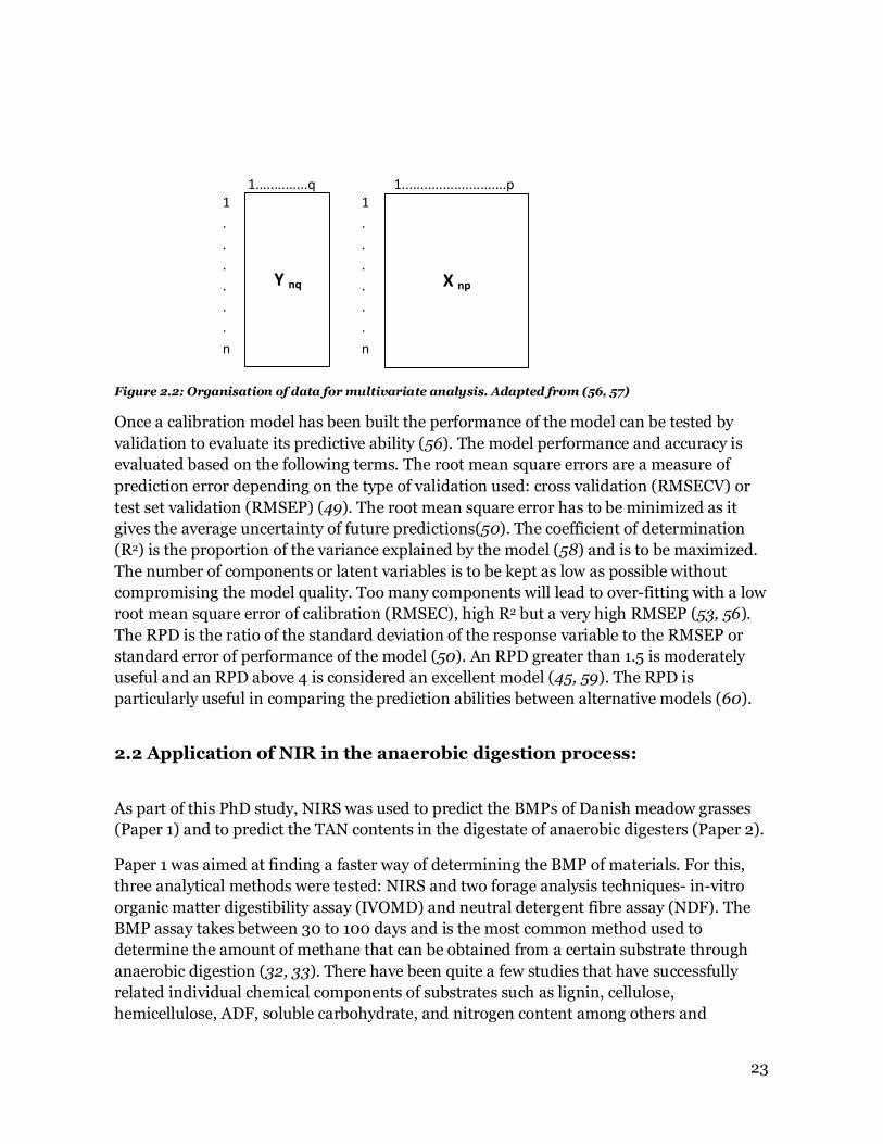
The data is organised in the form of matrices to facilitate analysis. If there are ‘n’ number
of objects, ‘p’ number of X-variables and ‘q’ number of Y- variables, the data matrices could
be represented as shown in Figure 2.2. The X matrix has n rows of spectral data and p
columns of spectral variables; each object is represented by one row containing p number
of spectral variables. Similarly the Y matrix has n rows, each row representing one object
with q dependent variables.
Using multivariate analysis techniques, calibration models are built by combining the p
measurements in X to give as good a prediction of Y as possible (57). This model is then
used to predict the Y value of new samples based on their spectra i.e. X values (57). In
other words, the spectral data are pre-processed if needed, and then related to a selected
reference variable using multivariate analytical methods. Based on the correlations from
these analyses, models to predict the reference variable are constructed.
Source Interferometer Sample Detector Amplifier Analog to
digital
converter
Computer
23
Figure 2.2: Organisation of data for multivariate analysis. Adapted from (56, 57)
Once a calibration model has been built the performance of the model can be tested by
validation to evaluate its predictive ability (56). The model performance and accuracy is
evaluated based on the following terms. The root mean square errors are a measure of
prediction error depending on the type of validation used: cross validation (RMSECV) or
test set validation (RMSEP) (49). The root mean square error has to be minimized as it
gives the average uncertainty of future predictions(50). The coefficient of determination
(R2) is the proportion of the variance explained by the model (58) and is to be maximized.
The number of components or latent variables is to be kept as low as possible without
compromising the model quality. Too many components will lead to over-fitting with a low
root mean square error of calibration (RMSEC), high R2 but a very high RMSEP (53, 56).
The RPD is the ratio of the standard deviation of the response variable to the RMSEP or
standard error of performance of the model (50). An RPD greater than 1.5 is moderately
useful and an RPD above 4 is considered an excellent model (45, 59). The RPD is
particularly useful in comparing the prediction abilities between alternative models (60).
2.2 Application of NIR in the anaerobic digestion process:
As part of this PhD study, NIRS was used to predict the BMPs of Danish meadow grasses
(Paper 1) and to predict the TAN contents in the digestate of anaerobic digesters (Paper 2).
Paper 1 was aimed at finding a faster way of determining the BMP of materials. For this,
three analytical methods were tested: NIRS and two forage analysis techniques- in-vitro
organic matter digestibility assay (IVOMD) and neutral detergent fibre assay (NDF). The
BMP assay takes between 30 to 100 days and is the most common method used to
determine the amount of methane that can be obtained from a certain substrate through
anaerobic digestion (32, 33). There have been quite a few studies that have successfully
related individual chemical components of substrates such as lignin, cellulose,
hemicellulose, ADF, soluble carbohydrate, and nitrogen content among others and
Y nq
X np
1..............q
1
.
.
.
.
.
.
n
1............................p
1
.
.
.
.
.
.
n

24
combinations of these components to their BMPs (33, 61, 62). Compared to the BMP assay
or the chemical analyses, NIRS is very quick and as mentioned earlier the NIRS method
does not require the use of chemicals and can be used online and inline.
The nutrition that ruminants can obtain from forage depends on the degradation of the
plant cell wall by the rumen microbes (63). The IVOMD which can be expressed in
percentage of dry matter (%DM), indicates the percentage of material that can be digested
by the ruminants and hence the nutritional value of that feed. Since the process is
anaerobic, it was interesting to see if the results of this assay would correlate to the BMP.
The NDF assay measures the cell wall components and includes cellulose hemicellulose
and lignin (64, 65). The pectic polysaccharides are not measured but since grasses have a
low pectin concentration in their cell walls, NDF is considered a good estimate of cell wall
contents in grasses (65). The aim was to see if just the cell wall contents, since it essentially
represents the lignocellulosic complex, could be used to determine the BMP of a material.
Paper 2 is focused on the application of NIRS in monitoring the anaerobic digestion
process. Anaerobic digesters, especially those using livestock wastes and those that operate
at thermophilic temperatures are susceptible to ammonia inhibition (42). Some studies
have successfully used NIRS to monitor VFA’s (40, 47, 66). Paper 2 investigates the use of
an NIR diffuse reflectance probe that can be directly fixed on to a reactor to predict the
TAN content of digestate.
2.3 Equipment and materials:
The spectrometer was a Bomem QFA Flex Fourier transform - NIR spectrometer (Q-
interline A/S, Copenhagen, Denmark). The detector that was used depended on the
material that was being scanned. The InAs detector was used for the meadow grass
experiment (Paper 1) while the InGaAs detector was used for the digestate samples (Paper
2).
Materials used: Dried meadow grass samples obtained from various locations in Denmark
were used to relate their BMP’s to their spectral data. Digestate samples from bench scale
continuous stirred tank reactors (CSTR) were used for the ammonia monitoring
experiment. More details regarding the materials can be found in Paper 1 and Paper 2.
2.4 Multi-variate data analysis software:
Two commercially available software, the Unscrambler ver. 9.8 software (CAMO Software
A/S, Oslo, Norway) and LatentiX software ver. 2.00 (Latent5, Copenhagen, Denmark)
were used for data analysis and for building models.
25
2.5 Data analysis:
Various multivariate analytical methods and data pre-processing methods were used to
derive useful conclusions from the large amount of spectral data that was obtained from
scanning the various samples. There are various multivariate analytical techniques
available like multiple regression, principle component regression (PC/MR) and partial
least squares regression(PLSR) (57). The multivariate methods used in this PhD study are
described in the following subsections.
Data pre-processing:
The data pre-processing methods available in the Unscrambler ver. 9.8 were used to
improve the models obtained from the spectral data. The pre-processing methods that
improved the models the most are described here. In Paper 1 the best results were obtained
with mean normalized data. Mean normalization is a row operation where each row of
spectral data is divided by its average value. The original values describing the object are
replaced by relative values (67). In Paper 2, standard normal variate (SNV)
transformations are used to remove the effects of scatter(68). In SNV transformations,
each spectrum is centered and then scaled by its own standard deviation (55).
Principal component analysis (PCA):
When dealing with large data matrices, PCA is used to reveal variables that describe some
inherent structure in the data and to reduce the dimension of the data without loss of
information (44, 69). This is done by finding a linear combination of data (a principal
component) that has maximum variance, and then the next linear combination that has
the second highest variance is determined and so on until most of the variance in the data
has been described by those components. In other words, the first component is a vector
that lies in the direction of the largest variance; the second is orthogonal to the first
component and lies in the direction of the next largest variance and so on. These principal
components are used to describe the data thus reducing the dimension of the data. PCA
separates the data structure from noise (66). It also groups objects with similar
characteristics together and aids in identifying outliers. PCA decomposes the X matrix into
two smaller matrices called the scores and the loadings (70). It is possible to have an
overview of the associations between objects and variables using the scores and loading
plots obtained from PCA (71).

26
Partial least squares (PLS) regression and interval PLS (iPLS):
PLS is useful where a large amount of independent variables (in this case spectral data) are
used to predict a set of dependent variables (BMP in Paper 1 and TAN in Paper 2). It can
analyze data that is highly correlated and noisy (72). Ordinary multiple regression is not
suited for spectral data as the spectral data are highly correlated (57). Unlike PC/MR, the
PLS method uses information from both the spectral data set and the dependent variable
data set to determine the PLS components/ latent variables and the components are
obtained by maximizing the covariance between the spectra and the dependent variable
(73). PLS assumes that the underlying set of latent variables for both the spectral data and
the response variable are the same (74). The purpose of PLS is to build a linear model that
can use spectral data to predict the dependent variable (75).
Interval partial least squares regression (iPLS) is a method that selects variables that are
most useful for a model by building local PLS models on equidistant sub-sections of the
spectrum and comparing the performance of these models in terms of RMSECV with the
global model (75). The output is graphical and it visually represents the wavelength ranges
that have been used for modelling (Paper 2). iPLS is a method that optimizes the predictive
power of PLSR (75).
2.6 Summary of results:
The results from the studies that have been done (Paper 1, Paper 2 and the Report) show
that NIRS is a promising analytical tool in process monitoring as well as feed input
management.
• The NIR prediction of the BMP of meadow grasses had an RPD of 1.75 which makes
it a moderately useful model that can discriminate between high and low values of
the response variable (45, 50). The NDF and IVOMD showed very little correlation
to the BMP (Paper 1).
• The study using NIRS to detect TAN in digestate was successful, and can in future
be optimized to be used as a monitoring tool (Paper2).
• The importance of choosing the right variables while building a model was also
demonstrated (Paper 2).
Further studies can be directed at building models to predict the BMP of other common
substrates that are used for biogas production. These models can be used to classify a
substrate as having a high or low BMP. By classifying the substrate and by recognizing
if the material has ammonia concentrations that are inhibitory, the feeding rate of the
substrate or in case of co-digestion plants, the ratio in which it is mixed, can be
27
controlled. As NIRS has been shown to predict TAN contents in a complex material
such as digestate (Paper 2), it could be used to screen manure based substrates for their
ammonia contents prior to loading into the reactor thus preventing the risk of
inhibition and to maintain an optimum C/N ratio. The results from the Report show
that the way the sample is presented to the NIR instrument is important, which
suggests that the model in Paper 2 could be improved further. While extremely good
results can be obtained in the laboratory by keeping conditions as similar as possible, it
would be better to mimic practical conditions even though the quality of the models
may degrade. If a model is to be applied to process monitoring it is important that the
calibration contains all ranges of the response variable that might be encountered and
that it includes all possible variations in conditions that might occur (76).
28
Chapter 3 – Pre-treatment of substrates
3.1 Necessity of pre-treatment
The use of agricultural and livestock waste for the production of biogas is often
uneconomical due to the content of recalcitrant organic matter. The economical
profitability of biogas plants that use such waste as primary feedstock depends on the
addition of other substrates with high methane yields (77). Biogas yield of pig and cow
manure is between 25 and 36 m3/tonne of fresh mass due to a low organic dry matter
content (2 to 10%) with a high fibre fraction (78). Manure based biogas plants in Germany
add co-substrates such as energy crops, waste from food and agricultural industries,
markets, canteens, and the municipal sector to improve profitability (78). Similarly most
large scale biogas plants in Denmark use manure as feedstock along with co-substrates
such as sewage sludge and industrial organic waste (77, 79).
Manure characteristics differ depending on various factors and therefore their methane
potentials differ as well. Some of the factors that affect the manure characteristics are, the
species, breed and growth stage of the animals, the feed being used, the amount and type
of bedding material, the stabling system used, and the method and period of storage (80).
The fibre fraction of manure consists mainly of undigested plant material, nutrients and
often includes bedding material (81). About 5 to 73% of the organic matter in manure
consists of lignocellulosic fibres that are recalcitrant to microbial degradation (62).
Agricultural residues such as straws, rice husk, and corn stover have high lignin
concentrations. Wheat has a lignin content of 15 to 19% whereas corn stover has been
reported to be about 19% lignin (77, 82). As mentioned in the introduction, the presence of
lignin creates a barrier for microbial degradation of the lignocellulosic complex and a
higher lignin content has been related to lower methane yields (62). Thus the use of
agricultural or livestock waste to produce biogas has to overcome the issue of
lignocellulose, to anaerobically convert as much of the volatile solids in the given
timeframe as possible.
Lignocellulosic content is a term used to describe the three dimensional composite
structural material in a plant cell wall, which is mainly 30 to 50% cellulose, 15 to 35%
hemicellulose and 10 to 30% lignin (82, 83). The lignocellulosic complex varies among
plant species and in addition the composition and percentages vary within the same plant
species depending on age, growth stage and other factors (84). Lignin is a phenolic
polymer and is not degradable by anaerobic processes, whereas the cellulose and
hemicellulose are carbohydrate polymers (82, 85). The lignin, cellulose and hemicellulose
are closely associated and form tight complexes, limiting the access of hydrolytic enzymes
to the cellulose and hemicellulose and slowing the rate of hydrolysis. Lignin is the natural
defence of plants against microbial attacks and hence some intervention is needed to break
29
down the lignocellulosic complex before it can be degraded anaerobically within a given
timeframe. Pre-treatments are aimed at removing or changing structural and
compositional constraints to improve the hydrolysis rate (86). An effective pre-treatment,
solubilises hemicellulose thus releasing sugars, decreases cellulose crystalinity, increases
the specific surface area and results in increased access of enzymes for hydrolysis, with
minimum formation of inhibitors and loss of substrate (77, 87).
3.2 Lignocellulosic components
Lignin
Lignin is an amorphous phenolic polymer usually made of three different phenylpropane
units (p-coumaryl, coniferyl and sinapyl alcohol) that are held together by different types
of linkages (88). Lignin provides rigidity, impermeablity and resistance to microbial
attacks and to oxidative stress to the plant cells (89). Higher proportion of lignin indicates
higher resistance to chemical and enzymatic degradation and lower methane potential of
susbtrates (62, 90). Solubilization of lignin occurs with alkaline agents and at temperatures
above 180°C (83, 91).
Cellulose
Cellulose is a linear polymer composed of cellobiose units (a glucose-glucose dimer) and
the hydrolysis of cellulose releases the individual glucose monomers: the process known as
saccharification (82). The cellulose chains are grouped together to form microfibrils and
the microfibrils are bunched together to form cellulose fibres (89). The amorphous and
crystalline nature of cellulose is attributed to the presence of inter-chain hydrogen bonds
within the microfibrils (89).
Hemicellulose
Hemicellulose is a carbohydrate polymer that surrounds the cellulose fibres and is made of
both five-carbon pentoses (xylose and arabinose) and six-carbon hexoses (galactose,
glucose and mannose) and acetylated sugars (82, 89, 90). Hemicellulose is highly
branched and amorphous and hence is easily hydrolysed compared to cellulose (82). The
hemicellulose composition differs in different biomasses (89). The solubilization of
hemicellulose depends on the pH and the moisture apart from temperature and under
neutral conditions solubilization of hemicellulose starts at 150°C (88).
30
3.3 Various methods of pre-treatment
The goal of pre-treatment methods applied to recalcitrant biomass is to alter the structure
and chemical properties of the biomass to improve the rates of degradability (92). Pre-
treatment methods can be classified as mechanical, thermal, chemical, biological and
combinations of these.
Mechanical
Mechanical pre-treatments, which are usually size reduction techniques, aim at increasing
the available surface area and reducing the cellulose crystalinity and the degree of
polymerization (88, 89). Coarse size reduction reduces the biomass size to about 10 to 50
mm, chipping reduces the size to 10 to 30 mm while grinding and milling can reduce the
sizes to between 0.2 to 2 mm (89). The advantages of this method are that there is no risk
of formation of inhibitory compounds, and there is improvement in the methane yield due
to size reduction in some cases, the main disadvantage is the high energy requirements
(88). In certain cases though, a minimal size reduction is required to overcome heat and
mass transfer problems in downstream processes (83).
Thermal
There are different ways of applying thermal pre-treatment to improve the hydrolysis rate
of lignocellulosic biomasses. Steam treatment - where the biomass is exposed to
temperatures up to 240°C and pressure for a few minutes (88). Steam explosion is similar
to steam treatment, except at the end of the pre-treatment period the pressure is released
suddenly, causing the disruption of the structure of the material (88, 93). Liquid hot water
treatment, where the water is maintained as a liquid at high temperatures (160 to 230°C)
and under high pressures (>5 MPa) (83, 88) or just thermal pre-treatment, an isochoric or
constant volume process, where the material is placed in a sealed container and heated
without applying extra external pressure (91). Another method is autohydrolysis, a process
that hydrolyzes hemicelluloses using highly pressurised liquid hot water at 200°C (86).
Chemical
Acid or alkali based pre-treatments can be used alone or in combination with thermal pre-
treatment. Acid based pre-treatments use either dilute or strong acids to hydrolyse the
hemicellulose content and to solubilize and precipitate lignin (88). Degradation products
such as furfurals or hydroxymethyl furfural (HMF) are formed during acid hydrolysis (83).
Although these compounds are inhibitory to methanogens, they adapt to them after
31
acclimatization, to a certain extent (88). The choice of acid is important, using sulphuric or
nitric acid introduces sulphates or nitrates into the system and reduces the methane
production (88).
Addition of acid to thermal pre-treatment catalyses the solubilization of hemicellulose and
could reduce the optimal pre-treatment temperature (88). In essence thermal pre-
treatments by themselves behave like dilute acid hydrolysis. Water at high temperatures
behaves as an acid and the hydrolysis reaction is catalysed by hydronium ions (H3O+), in
addition acetic acid is released from the hemicellulose fraction under high temperatures
adding to the effect(83, 86).
Alkali pre-treatment uses bases like calcium oxide, ammonia and sodium hydroxide to
solubilize lignin (83). In alkaline hydrolysis there is an increase in internal surface area of
the lignocellulosic material due to swelling induced by the alkali (89). This, along with
saponification of the intermolecular ester bonds that link hemicelluloses to other
components, leads to the separation of the lignin and the remaining carbohydrates (86).
Since the lignocellulosic composition varies among plant species, the efficiency of
separating the lignocellulosic components can be improved by exploiting these variations.
For example, the structure, composition and properties of lignocellulose from herbaceous
materials like wheat straw are very different from those of softwoods or hardwoods (94).
Alkaline pre-treatment methods are more effective on materials with low lignin contents
such as agricultural residues, herbaceous crops and hardwoods than on softwood which
has high lignin contents (95).
Biological
Biological pre-treatments mainly use fungi to degrade the lignin fraction (83). A wide
variety of fungi and bacteria are known to degrade lignin, of which white rot fungi are
thought to be the most efficient (84, 96, 97). Although the process is natural, and does not
require the use of chemicals or energy, which reduces the costs involved, the process is
slow and requires a longer residence time which is not practical for large scale applications
(83, 89).
3.4 Pre-treatment method used in this PhD study:
Paper 3 investigated the use of thermal pre-treatment in improving the BMPs of different
types of manure – cattle, dewatered pig and chicken manure. The process was carried out
under isochoric conditions where a known amount of material was sealed in a high
temperature and pressure reactor, and heated to the desired temperature, held at that
temperature for the required amount of time and then cooled down to about 30°C. Figure
32
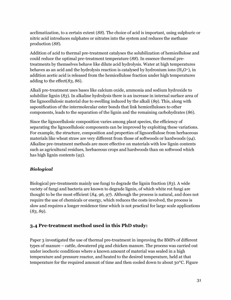
3.1 shows a typical heating and cooling curve for cow manure pre-treated at 100°C and at
200°C (Paper 3). The cooling was by a water bath with water at ambient temperature.
During these pre-treatment experiments, only the temperature was constantly monitored
and controlled, the pressure was not controlled.
Figure 3.1: A typical heating and cooling curve for the pressure vessel.
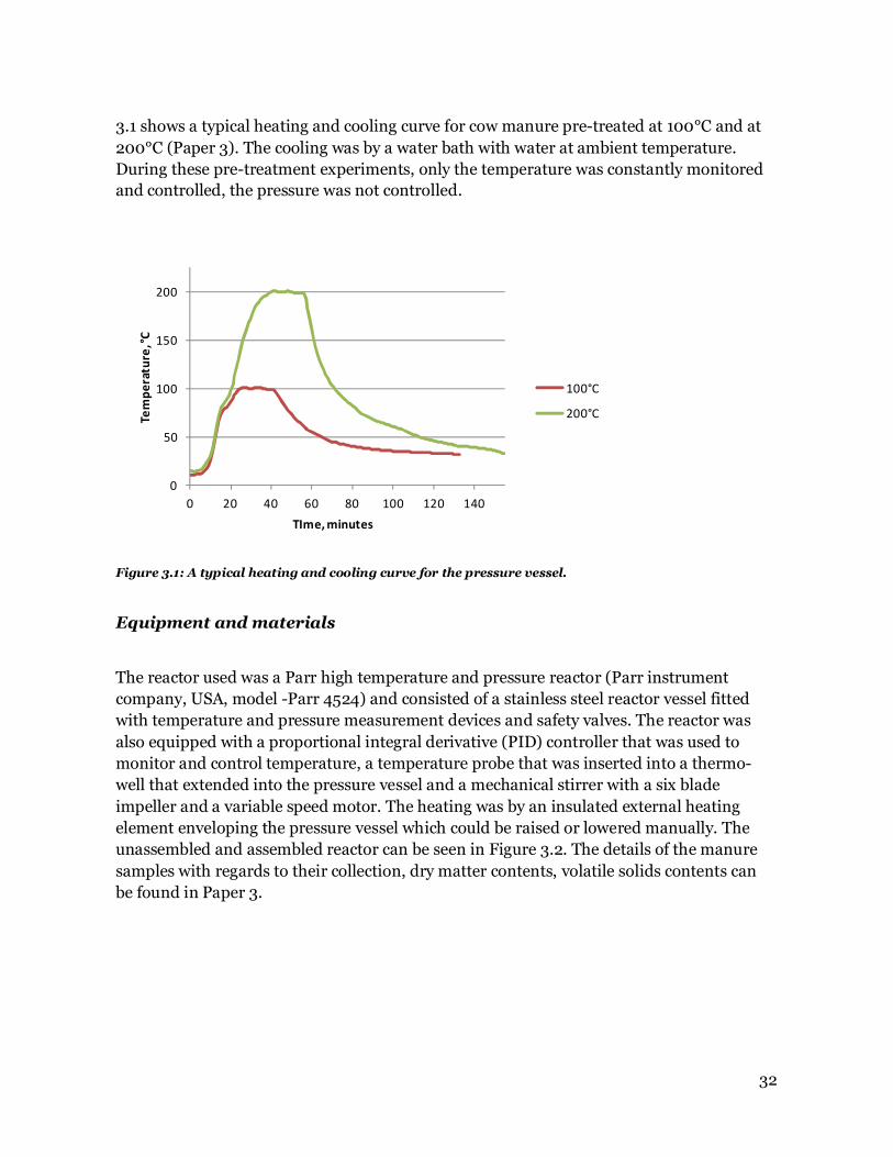
Equipment and materials
The reactor used was a Parr high temperature and pressure reactor (Parr instrument
company, USA, model -Parr 4524) and consisted of a stainless steel reactor vessel fitted
with temperature and pressure measurement devices and safety valves. The reactor was
also equipped with a proportional integral derivative (PID) controller that was used to
monitor and control temperature, a temperature probe that was inserted into a thermo-
well that extended into the pressure vessel and a mechanical stirrer with a six blade
impeller and a variable speed motor. The heating was by an insulated external heating
element enveloping the pressure vessel which could be raised or lowered manually. The
unassembled and assembled reactor can be seen in Figure 3.2. The details of the manure
samples with regards to their collection, dry matter contents, volatile solids contents can
be found in Paper 3.
0
50
100
150
200
0 20 40 60 80 100 120 140
Te
mp
era
ture
, °C
TIme, minutes
100°C
200°C
33
Figure 3.2: Parr high temperature and pressure vessel – unassembled and assembled
3.5 Severity factor
The results from Paper 3 when compared to those of other similar studies indicated that
the duration of the pre-treatment also influenced the effect of the pre-treatment on the
BMP along with the temperature used.
A term called severity factor is used to measure the severity of steam pre-treatment mainly
in the bioethanol industry (88). The severity factor (log R0) combines the temperature and
the duration of pre-treatment and is given by:
“log R0 = log(t × e((T-100)/14.75))”
- with ‘t’ in minutes and ‘T’ in degrees Celsius (88, 98).
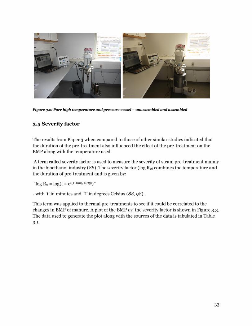
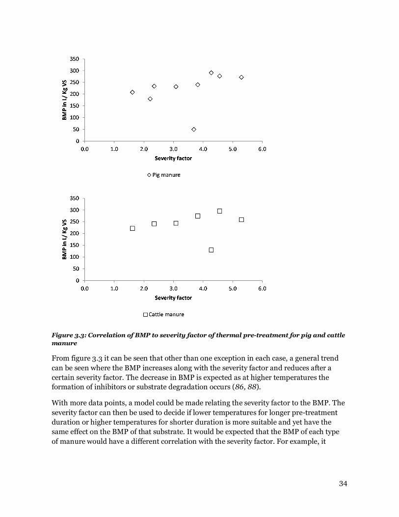
This term was applied to thermal pre-treatments to see if it could be correlated to the
changes in BMP of manure. A plot of the BMP vs. the severity factor is shown in Figure 3.3.
The data used to generate the plot along with the sources of the data is tabulated in Table
3.1.
34
Figure 3.3: Correlation of BMP to severity factor of thermal pre-treatment for pig and cattle
manure
From figure 3.3 it can be seen that other than one exception in each case, a general trend
can be seen where the BMP increases along with the severity factor and reduces after a
certain severity factor. The decrease in BMP is expected as at higher temperatures the
formation of inhibitors or substrate degradation occurs (86, 88).
With more data points, a model could be made relating the severity factor to the BMP. The
severity factor can then be used to decide if lower temperatures for longer pre-treatment
duration or higher temperatures for shorter duration is more suitable and yet have the
same effect on the BMP of that substrate. It would be expected that the BMP of each type
of manure would have a different correlation with the severity factor. For example, it
35
would be expected that the BMP-severity factor model of straw would be different from
that of dewatered pig manure.
Table 3.1: Data used to calculate the severity factor, along with the references for the sources
Reference Manure type Temperature
in °C Time in
minutes Severity
factor BMP in L/ Kg
VS (30 days)
(99) Dewatered pig manure 100 60 2.2 180
(99) Dewatered pig manure 150 60 3.7 50
Paper 3 Dewatered pig manure 100 15 1.6 208
Paper 3 Dewatered pig manure 125 15 2.3 234
Paper 3 Dewatered pig manure 150 15 3.1 232
Paper 3 Dewatered pig manure 175 15 3.8 240
Paper 3 Dewatered pig manure 200 15 4.6 277
Paper 3 Dewatered pig manure 225 15 5.3 272
(100) Pig manure 170 60 4.3 291
Paper 3 Cattle manure 100 15 1.6 222
Paper 3 Cattle manure 125 15 2.3 242
Paper 3 Cattle manure 150 15 3.1 244
Paper 3 Cattle manure 175 15 3.8 275
Paper 3 Cattle manure 200 15 4.6 296
Paper 3 Cattle manure 225 15 5.3 259
(100) Cattle manure 170 60 4.3 130
3.6 Summary of results
The effect of thermal pre-treatment was more pronounced in some manure types than
others. The effect mainly depended on the type of substrate, the pre-treatment
temperature and the pre-treatment duration.
• Dewatered pig manure showed improved BMP from pre-treatment temperatures of
125°C onwards
• Cattle manure needed pre-treatment temperatures above 175°C for improved BMP
• Chicken manure showed no improvement in the BMP due to thermal pre-treatment
but showed a decrease at 225°C
• In cases where significant increases were seen due to the pre-treatment, the biggest
difference was seen within the first 30 days. Increases in initial methane production
rates are important when considering full scale biogas plants.
• For practical applications, it seems thermal pre-treatment can be applied to
dewatered pig manure, as, among the three manure types tested, it improves
significantly at lower temperatures in comparison to the other two manures. A
proper cost benefit analysis will be required to see if the pre-treatment can improve
the economic profitability of the biogas plant.

36
One main aspect that is to be considered with thermal pre-treatment is the energy
balance. Thermal pre-treatments have been applied to full scale operations to improve
their economic profitability (100, 101). It is important to ensure that the use of energy
for the pre-treatment is justified by more than an equivalent increase in energy in
terms of methane yields. Thermal pre-treatments can be justified where waste heat is
available and where the heat used for pre-treatment can be recycled or where the
energy gain due to the pre-treatment is much higher than the extra energy input that is
required.

37
Appendix
38
Paper 1
Comparison of near infra-red spectroscopy, neutral detergent fibre assay
and in-vitro organic matter digestibility assay for rapid determination of
the biochemical methane potential of meadow grasses
Chitra Sangaraju Raju, Alastair James Ward, Lisbeth Nielsen, Henrik Bjarne Møller
Published
Journal - Bioresource Technology 102 (2011) 7835–7839

Paper not inserted due to copyrights held by the publisher

49
Paper 2
NIR monitoring of ammonia in anaerobic digesters using diffuse reflectance
probe
Chitra S Raju, Mette Marie Løkke, Sutaryo Sutaryo, Alastair J. Ward, Henrik B. Møller
Published
Journal – Sensors 12 (2012) 2340-2350

Sensors 2012, 12, 2340-2350; doi:10.3390/s120202340
sensors ISSN 1424-8220
www.mdpi.com/journal/sensors Article
NIR Monitoring of Ammonia in Anaerobic Digesters Using a
Diffuse Reflectance Probe
Chitra S. Raju 1,*, Mette Marie Løkke
2, Sutaryo Sutaryo
1, Alastair J. Ward
1 and
Henrik B. Møller 1
1 Department of Engineering, Aarhus University, Blichers Allé 20, Tjele DK 8830, Denmark;
E-Mails: [email protected] (S.S.); [email protected] (A.J.W.);
[email protected] (H.B.M.) 2 Department of Food Science, Aarhus University, Kirstinebjergvej 10, Årslev DK 5792, Denmark;
E-Mail: [email protected]
* Author to whom correspondence should be addressed; E-Mail: [email protected];
Tel.: +45-8715-7874.
Received: 18 January 2012; in revised form: 16 February 2012 / Accepted: 16 February 2012 /
Published: 21 February 2012
Abstract: The feasibility of using a diffuse reflectance probe attached to a near infrared
spectrometer to monitor the total ammonia nitrogen (TAN) content in an anaerobic digester
run on cattle manure was investigated; as a previous study has indicated that this probe can
be easily attached to an anaerobic digester. Multivariate modelling techniques such as partial
least squares regression and interval partial least squares methods were used to build models.
Various data pre-treatments were applied to improve the models. The TAN concentrations
measured were in the range of 1.5 to 5.5 g/L. An R2 of 0.91 with an RMSEP of 0.32 was
obtained implying that the probe could be used for monitoring and screening purposes.
Keywords: NIRS; biogas; ammonia; inhibition; monitoring; manure; PLS; iPLS
1. Introduction
Intensive farming methods generate large amounts manure that need safe disposal. In Denmark,
more than 33 million tonnes of manure are produced per annum [1]. Current manure management
strategies involve spreading of manure on agricultural fields to recycle the nutrients, aerobic treatment,
separation of the solid and liquid fractions, composting and anaerobic digestion among others [2].
OPEN ACCESS
Sensors 2012, 12 2341
Denmark has many full-scale biogas plants that use livestock manure as substrate along with organic
wastes from industries [3]. Livestock wastes contain ammonia, which is inhibitory to anaerobic
digestion, and contain compounds like urea and proteins that will degrade into ammonia [4]. Ammonia
is present in the form of the ammonium ion (NH4+) and free ammonia (NH3), of which the free
ammonia (FA) is suspected to be the main cause for inhibition [5]. The ammonium ion and free
ammonia exist in equilibrium, and the equilibrium depends on the temperature and pH. A decrease in
pH reduces the amount of free ammonia. When a process is inhibited by free ammonia, the
methanogens are affected, and consequently the volatile fatty acids (VFA) accumulate reducing the
pH, this in turn reduces the free ammonia concentration [4]. This leads to a stable condition but at a
sub-optimal level called an inhibited steady state. Total ammonia nitrogen (TAN) levels of more than
4 g N/L were found to cause inhibition; levels beyond this showed stable biogas production after an
initial adaptation period but this biogas yield was lower than that of uninhibited reactors [4]. Livestock
manure can often have more than 4 g N/L of ammonia, especially in the case of swine manure and
poultry manure [4], the ammonia concentrations can also be high in anaerobic co-digestion plants that
mix high protein wastes to their substrates. Thus, monitoring the ammonia content of the slurry in
anaerobic digesters is an important aspect of process control and in managing the substrate feeding rate.
Ammonia content is usually measured and monitored by laboratory analysis such as colorimetry.
This procedure involves the use of reagents, is time consuming and is not practical for process control.
Near infrared (NIR) spectroscopy has been used to monitor various process indicators in the anaerobic
digestion process. Earlier experiments using Trans-flexive NIR Spectroscopy (TENIRS) has shown
good results in predicting the ammonia contents in an anaerobic digester [6]. Another study that
showed good results in applying NIR spectroscopy to predict ammonia, used the polyethylene bag
method where a sample of cattle manure was filled into a polyethylene bag and then pressed on to the
surface of the scanning window of the NIR spectrometer [7]. However, the TENIRS requires the use of
a macerator to reduce the size of the slurry particles to below 3 mm before the sample can be sent
through it. The polyethylene bag method requires the sample to be taken out of the reactor and then
analysed elsewhere.
A previous study used a reflectance probe to monitor the propionate contents of a small
continuously stirred reactor successfully [8]. It has also been shown that the probe can be directly fitted
on to a reactor without major changes to the reactor body [9]. The aim of this study was to investigate
the feasibility of predicting the ammonia content of manure using a diffuse reflectance probe. The
reflectance probe also offers easy maintenance and unlike transmission spectroscopy does not depend
on the transmission path lengths. A drawback of the reflectance probe is that more scatter is expected,
and therefore more noise will be added to the spectra. This study describes the first step which is to
determine if the diffuse reflectance probe can actually be used to determine the total ammonia nitrogen
(TAN) concentrations in a complex material such as slurry from an anaerobic digester and if feasible,
future studies can be directed at fitting the probe onto a full scale anaerobic reactor and test its
performance. The slurry samples were scanned offline, using the diffuse reflectance probe. The
spectral data was analysed using multivariate analysis and models relating the spectral data to the TAN
contents were developed. Manure or slurry samples are a matrix of particles of different sizes and as a
consequence, measurements based on reflectance mode will have variation in light scattering (i.e.,
wavelength dependent path length variation) between samples which can negatively affect the
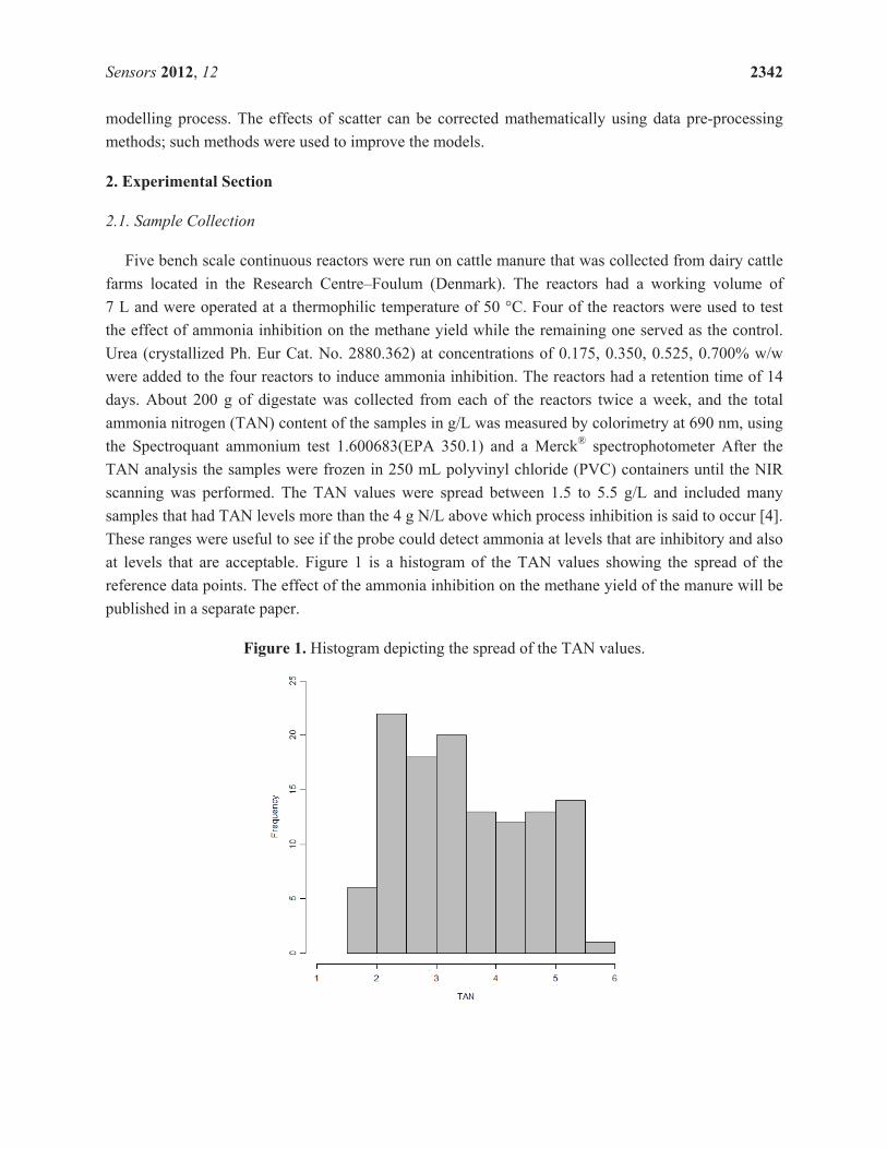
Sensors 2012, 12 2342
modelling process. The effects of scatter can be corrected mathematically using data pre-processing
methods; such methods were used to improve the models.
2. Experimental Section
2.1. Sample Collection
Five bench scale continuous reactors were run on cattle manure that was collected from dairy cattle
farms located in the Research Centre–Foulum (Denmark). The reactors had a working volume of
7 L and were operated at a thermophilic temperature of 50 °C. Four of the reactors were used to test
the effect of ammonia inhibition on the methane yield while the remaining one served as the control.
Urea (crystallized Ph. Eur Cat. No. 2880.362) at concentrations of 0.175, 0.350, 0.525, 0.700% w/w
were added to the four reactors to induce ammonia inhibition. The reactors had a retention time of 14
days. About 200 g of digestate was collected from each of the reactors twice a week, and the total
ammonia nitrogen (TAN) content of the samples in g/L was measured by colorimetry at 690 nm, using
the Spectroquant ammonium test 1.600683(EPA 350.1) and a Merck® spectrophotometer After the
TAN analysis the samples were frozen in 250 mL polyvinyl chloride (PVC) containers until the NIR
scanning was performed. The TAN values were spread between 1.5 to 5.5 g/L and included many
samples that had TAN levels more than the 4 g N/L above which process inhibition is said to occur [4].
These ranges were useful to see if the probe could detect ammonia at levels that are inhibitory and also
at levels that are acceptable. Figure 1 is a histogram of the TAN values showing the spread of the
reference data points. The effect of the ammonia inhibition on the methane yield of the manure will be
published in a separate paper.
Figure 1. Histogram depicting the spread of the TAN values.
Sensors 2012, 12 2343
2.2. NIR Scanning
The NIR scanning was performed using a Bomem QFA Flex Fourier Transform spectrometer fitted
with an InGaAs detector (Q-interline A/S, Copenhagen, Denmark). The diffuse reflectance probe that
was used (QIA2050, also from Q-interline A/S) had a stainless steel body with a 5 mm sapphire window
embedded into it and scanned in the range of 833.3 nm to 2,500 nm (12,000 cm 1 to 4,000 cm 1). The
probe is specifically optimized for materials with high scatter like slurry from anaerobic digesters.
The NIR scanning, as mentioned earlier, was performed offline. The frozen digestate samples were
first brought to room temperature (19 to 20 °C) by thawing at room temperature overnight. The NIR
probe was rinsed with de-ionized water, wiped clean with a tissue and then placed into the PVC
container containing the digestate sample and clamped into position using a laboratory clamp stand
such that there was at least 2 cm of sample beneath it, ensuring that the position was the same for every
sample. An agitator was immersed parallel alongside the probe and the digestate sample was mixed at
190 rotations per minute (rpm) to make sure that enough sample passed in front of the scanning
window of the NIR probe. The speed of the agitator was optimized by trying different rpm settings to
ensure that there was no bubble formation which would negatively impact the scan while ensuring the
sample did not settle. For each sample, the measurement took about 80 s and consisted of 256 scans
which were then averaged for that particular sample. A total of 119 manure samples were scanned in a
time-span of two days. The background scan was measured against a white spectralon disk.
2.3. Model Calibration and Validation
NIR spectra are often noisy [10] due to various reasons, including instrument noise and high
absorbing materials, and detector performance. The entire spectra, obtained from the NIR spectrometer
amounted to 1,006 spectral variables. A lot of the variables were noisy due to high absorbance in
wavelengths above 1,800 nm and due to low detector sensitivity to wavelengths below 900 nm. These
areas were consequently cropped. There is often offset and slope variation between NIR spectra of
samples that have equal analyte concentration but different light scattering properties. Light scattering
differences in spectra can be minimized by data pre-processing.
Data pre-processing is therefore a necessary step before modelling and can be classified into two
main types. The first are scatter correcting methods such as multiplicative scatter correction (MSC),
extended MSC (EMSC), standard normal variate (SNV), de-trending, baseline offset correction (BOC)
and normalization. The second are spectral derivative pre-processing methods such as Norris-Gap
(NG) and Savitzky-Golay (SG) polynomial derivatives. The data pre-processing methods available in
the Unscrambler Version 9.8 software were applied to the spectral data and using the pre-processed
data, models to predict the TAN content were developed.
Two modelling methods: Partial least squares regression (PLS) and interval partial least squares
(iPLS) were used to relate the spectral variables obtained from the NIR to the reference variable (the
measured TAN values).
The commercially available Unscrambler Version 9.8 software (CAMO Software A/S, Oslo, Norway)
was used to develop the PLS models. The PLS is based on the regression method developed by Herman
Wold [11]. Each model was validated by both full cross validation and test set validation. Full or

Sensors 2012, 12 2344
leave-one-out cross validation is a model validation method where one sample is left out iteratively and a
calibration model is built, and then the sample that was left out is predicted using this model. The
iteration is continued until all samples are left out of the calibration set once. For the test set validation
the data set was divided into a calibration dataset and a validation dataset that both covered the range of
ammonia levels: the data was listed according to the ammonia level, and every fourth sample was added
to the test set (29 samples) and the rest of the samples were included into the calibration set (90 samples).
The other method used for modelling was the iPLS which is a graphically oriented local modelling
procedure [12]. The iPLS builds local models on sub-intervals of the whole spectrum and selects the
optimum sub-intervals in the spectral data to give precision prediction models [12,13]. Each
sub-interval contains a selected number of spectral variables. The iPLS models were built using the PLS
toolbox Version 6.2.1 (Eigenvector Research Inc., Wenatchee, WA, USA) in Matlab Version 7.12
(MathWorks, Natick, MA, USA). The iPLS was run using forward selection on raw and on SNV
pre-processed spectra with a sub-interval size of 30 variables and a maximum of four PLS components
(or latent variables) were allowed. To decide upon the number of components that could be used, the
number of components was varied and looking at the RMSEP of the full model it was found that there
was no advantage in using more than four components. For validation during iPLS optimization, full
cross validation was used. When the optimum interval combination was found, the model was
validated using the test set.
The prediction performance of the models was evaluated based on their modelling parameters: the
coefficient of determination (R2), the root mean square error of prediction (RMSEP) and by their residual
prediction deviation (RPD) which is the ratio of the standard deviation to the RMSEP [14]. The number
of principal components used to construct the model was also used as an indicator. High R2 and RPD
values, minimum number of components possible and low RMSEP values indicated a good model.
In general, eliminating redundant variables and basing models on the variables that are significant
will give lower estimation errors [15]. The iPLS automatically provides the variables that correlate the
most to the reference variable. In the case of PLS, once the best possible model was built, the number
of spectral variables was reduced by using Marten’s uncertainty test function [16] to see if the model
could be improved further by removing variables that are not important to the model. The uncertainty
test function is available in the Unscrambler Version 9.8 software and uses the jack-knifing method to
separate the unimportant variables from the useful ones hence simplifying the model. The reduced set
of variables was used to build a new model and then the uncertainty test was once again used to reduce
the variables further. This iterative approach was continued till the modelling parameters began to
deteriorate. The uncertainty test was also applied on the entire spectral range to investigate if the
results, after removing the unimportant variables, would be comparable to those of the best models
obtained by other methods.
3. Results and Discussion
The validation statistics including the modelling parameters of selected models are listed in Table 1.
Models 1 to 6 are the PLS models while models 7 and 8 are from iPLS. From the Figure 1 it can be
seen that the frequency of the TAN values is not even. An even spread of values would give a more
robust calibration model [17].
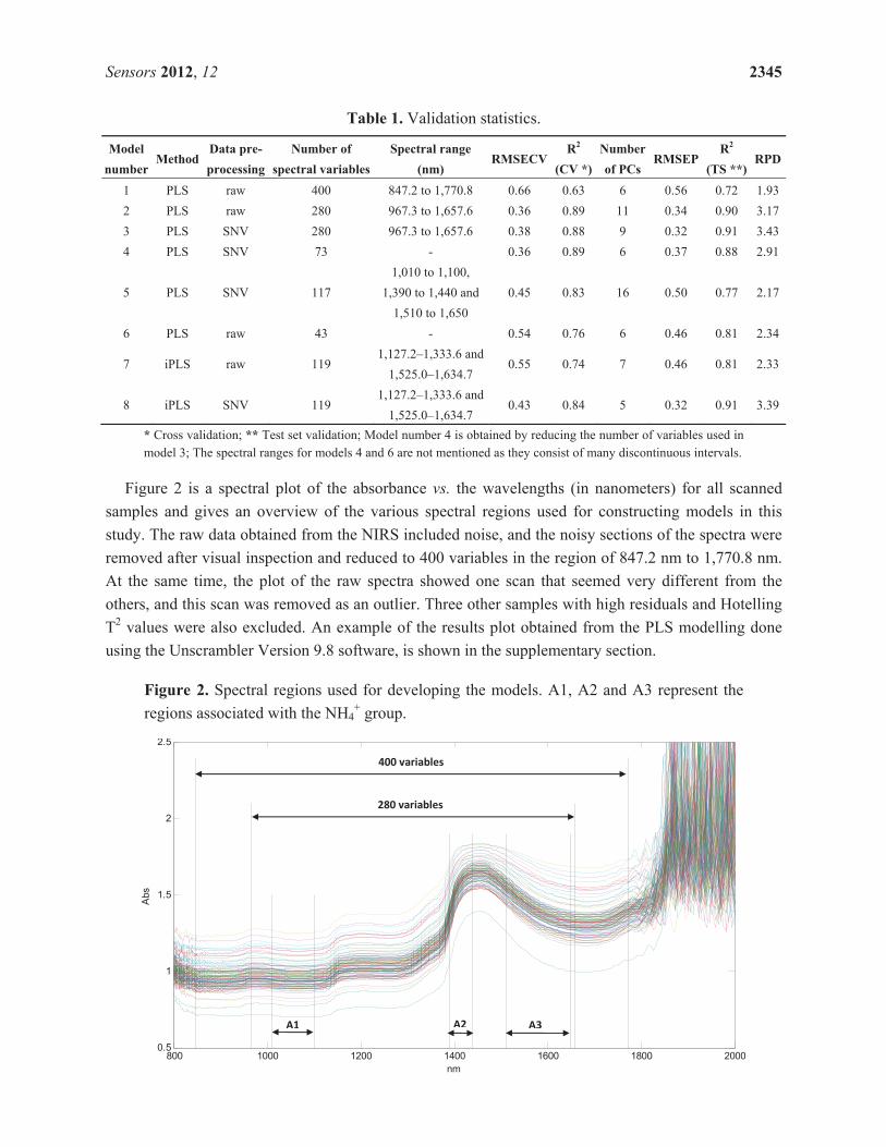
Sensors 2012, 12 2345
Table 1. Validation statistics.
Model
number Method
Data pre-
processing
Number of
spectral variables
Spectral range
(nm) RMSECV
R2
(CV *)
Number
of PCs RMSEP
R2
(TS **)RPD
1 PLS raw 400 847.2 to 1,770.8 0.66 0.63 6 0.56 0.72 1.93
2 PLS raw 280 967.3 to 1,657.6 0.36 0.89 11 0.34 0.90 3.17
3 PLS SNV 280 967.3 to 1,657.6 0.38 0.88 9 0.32 0.91 3.43
4 PLS SNV 73 - 0.36 0.89 6 0.37 0.88 2.91
5 PLS SNV 117
1,010 to 1,100,
1,390 to 1,440 and
1,510 to 1,650
0.45 0.83 16 0.50 0.77 2.17
6 PLS raw 43 - 0.54 0.76 6 0.46 0.81 2.34
7 iPLS raw 119 1,127.2–1,333.6 and
1,525.0–1,634.7 0.55 0.74 7 0.46 0.81 2.33
8 iPLS SNV 119 1,127.2–1,333.6 and
1,525.0–1,634.7 0.43 0.84 5 0.32 0.91 3.39
* Cross validation; ** Test set validation; Model number 4 is obtained by reducing the number of variables used in
model 3; The spectral ranges for models 4 and 6 are not mentioned as they consist of many discontinuous intervals.
Figure 2 is a spectral plot of the absorbance vs. the wavelengths (in nanometers) for all scanned
samples and gives an overview of the various spectral regions used for constructing models in this
study. The raw data obtained from the NIRS included noise, and the noisy sections of the spectra were
removed after visual inspection and reduced to 400 variables in the region of 847.2 nm to 1,770.8 nm.
At the same time, the plot of the raw spectra showed one scan that seemed very different from the
others, and this scan was removed as an outlier. Three other samples with high residuals and Hotelling
T2 values were also excluded. An example of the results plot obtained from the PLS modelling done
using the Unscrambler Version 9.8 software, is shown in the supplementary section.
Figure 2. Spectral regions used for developing the models. A1, A2 and A3 represent the
regions associated with the NH4+ group.
800 1000 1200 1400 1600 1800 2000
0.5
1
1.5
2
2.5
nm
Abs
A1 A2 A3
280 variables
400 variables
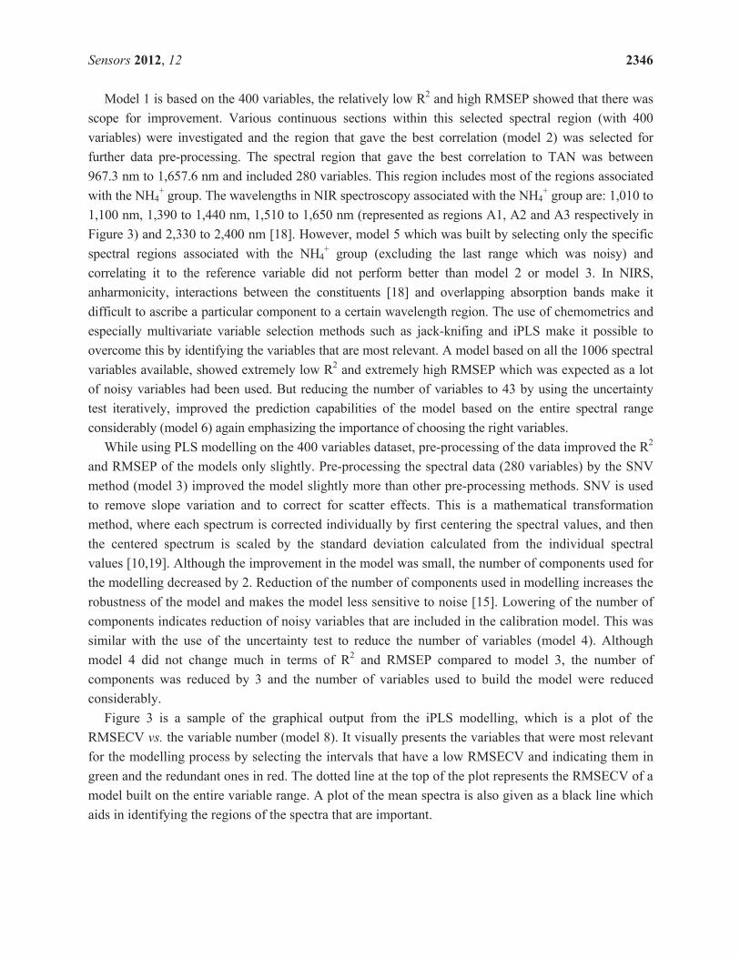
Sensors 2012, 12 2346
Model 1 is based on the 400 variables, the relatively low R2 and high RMSEP showed that there was
scope for improvement. Various continuous sections within this selected spectral region (with 400
variables) were investigated and the region that gave the best correlation (model 2) was selected for
further data pre-processing. The spectral region that gave the best correlation to TAN was between
967.3 nm to 1,657.6 nm and included 280 variables. This region includes most of the regions associated
with the NH4+ group. The wavelengths in NIR spectroscopy associated with the NH4
+ group are: 1,010 to
1,100 nm, 1,390 to 1,440 nm, 1,510 to 1,650 nm (represented as regions A1, A2 and A3 respectively in
Figure 3) and 2,330 to 2,400 nm [18]. However, model 5 which was built by selecting only the specific
spectral regions associated with the NH4+ group (excluding the last range which was noisy) and
correlating it to the reference variable did not perform better than model 2 or model 3. In NIRS,
anharmonicity, interactions between the constituents [18] and overlapping absorption bands make it
difficult to ascribe a particular component to a certain wavelength region. The use of chemometrics and
especially multivariate variable selection methods such as jack-knifing and iPLS make it possible to
overcome this by identifying the variables that are most relevant. A model based on all the 1006 spectral
variables available, showed extremely low R2 and extremely high RMSEP which was expected as a lot
of noisy variables had been used. But reducing the number of variables to 43 by using the uncertainty
test iteratively, improved the prediction capabilities of the model based on the entire spectral range
considerably (model 6) again emphasizing the importance of choosing the right variables.
While using PLS modelling on the 400 variables dataset, pre-processing of the data improved the R2
and RMSEP of the models only slightly. Pre-processing the spectral data (280 variables) by the SNV
method (model 3) improved the model slightly more than other pre-processing methods. SNV is used
to remove slope variation and to correct for scatter effects. This is a mathematical transformation
method, where each spectrum is corrected individually by first centering the spectral values, and then
the centered spectrum is scaled by the standard deviation calculated from the individual spectral
values [10,19]. Although the improvement in the model was small, the number of components used for
the modelling decreased by 2. Reduction of the number of components used in modelling increases the
robustness of the model and makes the model less sensitive to noise [15]. Lowering of the number of
components indicates reduction of noisy variables that are included in the calibration model. This was
similar with the use of the uncertainty test to reduce the number of variables (model 4). Although
model 4 did not change much in terms of R2 and RMSEP compared to model 3, the number of
components was reduced by 3 and the number of variables used to build the model were reduced
considerably.
Figure 3 is a sample of the graphical output from the iPLS modelling, which is a plot of the
RMSECV vs. the variable number (model 8). It visually presents the variables that were most relevant
for the modelling process by selecting the intervals that have a low RMSECV and indicating them in
green and the redundant ones in red. The dotted line at the top of the plot represents the RMSECV of a
model built on the entire variable range. A plot of the mean spectra is also given as a black line which
aids in identifying the regions of the spectra that are important.
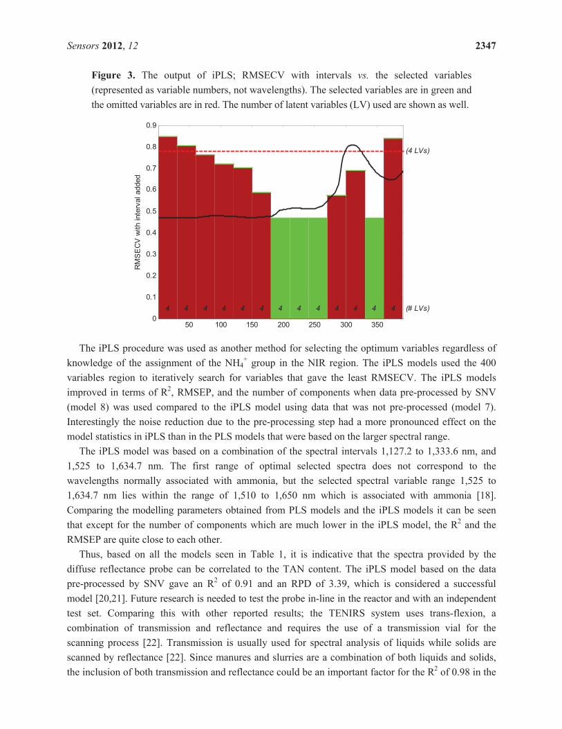
Sensors 2012, 12 2347
Figure 3. The output of iPLS; RMSECV with intervals vs. the selected variables
(represented as variable numbers, not wavelengths). The selected variables are in green and
the omitted variables are in red. The number of latent variables (LV) used are shown as well.
The iPLS procedure was used as another method for selecting the optimum variables regardless of
knowledge of the assignment of the NH4+ group in the NIR region. The iPLS models used the 400
variables region to iteratively search for variables that gave the least RMSECV. The iPLS models
improved in terms of R2, RMSEP, and the number of components when data pre-processed by SNV
(model 8) was used compared to the iPLS model using data that was not pre-processed (model 7).
Interestingly the noise reduction due to the pre-processing step had a more pronounced effect on the
model statistics in iPLS than in the PLS models that were based on the larger spectral range.
The iPLS model was based on a combination of the spectral intervals 1,127.2 to 1,333.6 nm, and
1,525 to 1,634.7 nm. The first range of optimal selected spectra does not correspond to the
wavelengths normally associated with ammonia, but the selected spectral variable range 1,525 to
1,634.7 nm lies within the range of 1,510 to 1,650 nm which is associated with ammonia [18].
Comparing the modelling parameters obtained from PLS models and the iPLS models it can be seen
that except for the number of components which are much lower in the iPLS model, the R2 and the
RMSEP are quite close to each other.
Thus, based on all the models seen in Table 1, it is indicative that the spectra provided by the
diffuse reflectance probe can be correlated to the TAN content. The iPLS model based on the data
pre-processed by SNV gave an R2 of 0.91 and an RPD of 3.39, which is considered a successful
model [20,21]. Future research is needed to test the probe in-line in the reactor and with an independent
test set. Comparing this with other reported results; the TENIRS system uses trans-flexion, a
combination of transmission and reflectance and requires the use of a transmission vial for the
scanning process [22]. Transmission is usually used for spectral analysis of liquids while solids are
scanned by reflectance [22]. Since manures and slurries are a combination of both liquids and solids,
the inclusion of both transmission and reflectance could be an important factor for the R2 of 0.98 in the
50 100 150 200 250 300 3500
0.1
0.2
0.3
0.4
0.5
0.6
0.7
0.8
0.9
(4 LVs)
(# LVs)
RM
SE
CV
with inte
rval added
4 4 4 4 4 4 4 4 4 4 4 4 4
Sensors 2012, 12 2348
TENIRS experiment. One disadvantage of using a transmission vial for the measurements is that it is
susceptible to clogging and to the formation of deposits. These lead to inaccuracies, due to a change in
the transmission path length which is vital to the calculations involving the received signal. The diffuse
reflectance probe does not have this problem.
High VFA concentrations cause inhibition, as the methanogens are sensitive to pH changes.
Changes in VFA concentration is also indicative of process imbalances, as any inhibition of
methanogens will lead to VFA accumulation. Previous studies using the diffuse reflectance probe in an
anaerobic digester have shown that it can also be used to predict the VFA concentrations [8,9] and can
thus be used to monitor VFA along with TAN. Apart from a monitoring system that could indicate
inhibitory levels of TAN content, the NIR probe could also be used to screen manure based substrates
for their TAN contents prior to loading into the reactor thus preventing the risk of inhibition. It can be
used to maintain an optimum C/N ratio, between 20/1 and 30/1, which is another way of preventing
ammonia accumulation and improving digester performance [23]. The use of NIR in predicting the
amount of TAN will also aid in feed input management especially while dealing with feedstock that is
high in protein and TAN content. In a previous study, NIR spectroscopy has been used to predict the
biochemical methane potential (BMP) of meadow grass based substrates [24]. If further studies
indicate that the diffuse reflectance probe can be calibrated to predict the BMP of manure based
substrates, the probe could serve multiple purposes in the process control of anaerobic digesters.
4. Conclusions
The models obtained were successful and thus the diffuse reflectance probe is promising as an
online ammonia monitoring tool for materials such as manure and digestates from anaerobic digesters.
Based on the spectra obtained from the probe, PLS and iPLS gave similar models, except iPLS used
lesser number of components indicating a more robust model. Pre-processing of the data also reduced
the number of components in the models when compared to models that were based on raw data.
Selecting the correct range of spectra that would be used in the model, however, proved to be very
important in this process.
References
1. Petersen, J.; Sørensen, P. Fertilizer Value of Nitrogen in Animal Manures-Basis for
Determination of a Legal Substitution Rate; Det Jordbrugsvidenskabelige Fakultet, Aarhus
University: Aarhus, Denmark, 2008.
2. Burton, C.H.; Turner, C. Manure Management—Treatment Strategies for Sustainable Agriculture,
2nd ed.; Silsoe Research Institute: Bedford, UK, 2003.
3. Angelidaki, I.; Ahring, B.K. Methods for increasing the biogas potential from the recalcitrant
organic matter contained in manure. Water Sci. Technol. 2000, 41, 189–194.
4. Angelidaki, I.; Ahring, B.K. Thermopihilic anaerobic digestion of livestock waste: The effect of
ammonia. Appl. Microbiol. Biotechnol. 1993, 38, 560–564.
5. Chen, Y.; Cheng, J.J.; Creamer, K.S. Inhibition of anaerobic digestion process: A review.
Bioresour. Technol. 2008, 99, 4044–4064.

Sensors 2012, 12 2349
6. Holm-Nielsen, J.B.; Andree, H. Lindorfer, H.; Esbensen, K.H. Transflexive embedded near
infrared monitoring for key process intermediates in anaerobic digestion/biogas production.
J. Near Infrared Spectrosc. 2007, 15, 123–135.
7. Reeves, J.B., III; Van Kessel, J.S. Near-infrared spectroscopic determination of carbon, total
nitrogen, and ammonium-N in dairy manures. J. Dairy Sci. 2000, 83, 1829–1836.
8. Hansson, M.; Nordberg, Å.; Mathisen, B. On-line NIR monitoring during anaerobic treatment of
municipal solid waste. Water Sci. Technol. 2003, 48, 9–13.
9. Ward, A.J.; Raju, C.S.; Møller, H.B. Using Near Infrared Spectroscopy to Predict Volatile Fatty
Acids in Biogas Processes Utilising Different Feedstocks. In Proceedings of the 14th Ramiran
International Conference, Lisbon, Portugal, 12–15 September 2010.
10. Rinnan, Å.; van den Berg, F.; Engelsen, S.B. Review of the most common pre-processing
techniques for near-infrared spectra. Trac-Trends Anal. Chem. 2009, 28, 1201–1222.
11. Wold, S.; Sjöström, M.; Eriksson, L. PLS-regression: A basic tool of chemometrics.
Chemom. Intell. Lab. Syst. 2001, 58, 109–130.
12. Nørgaard, L.; Saudland, A.; Wagner, J.; Nielsen, J.P.; Munck, L.; Engelsen, S.B. Interval partial
least-squares regression (iPLS): A comparative chemometric study with an example from
near-infrared spectroscopy. Appl. Spectrosc. 2000, 54, 413–419.
13. Zachariassen, C.B.; Larsen, J.; van den Berg, F.; Balling Engelsen, S. Use of NIR spectroscopy
and chemometrics for on-line process monitoring of ammonia in Low Methoxylated Amidated
pectin production. Chemom. Intell. Lab. Syst. 2005, 76, 149–161.
14. Lomborg, C.J.; Holm-Nielsen, J.B.; Oleskowicz-Popiel, P.; Esbensen, K.H. Near infrared and
acoustic chemometrics monitoring of volatile fatty acids and dry matter during co-digestion of
manure and maize silage. Bioresour. Technol. 2009, 100, 1711–1719.
15. Esbensen, K.H. Multivariate Data Analysis—In Practice. An Introduction to Multivariate Data
Analysis and Experimental Design, 5th ed.; CAMO: Oslo, Norway, 2009.
16. Martens, H.; Martens, M. Modified Jack-knife estimation of parameter uncertainty in bilinear
modelling by partial least squares regression (PLSR). Food Qual. Prefer. 2000, 11, 5–16.
17. Næs, T.; Isaksson, T.; Fearn, T.; Davies, T. A User-Friendly Guide to Multivariate Calibration
and Classification; NIR Publications: West Sussex, UK, 2007.
18. Williams, P.; Norris, K. Near-Infrared Technology in the Agricultural and Food Industries;
American Association of Cereal Chemists Inc.: St. Paul, MN, USA, 1987.
19. Barnes, R.J.; Dhanoa, M.S.; Lister, S.J. Standard normal variate transformation and de-trending of
near-infrared diffuse reflectance spectra. Appl. Spectrosc. 1989, 43, 772–777.
20. Malley, D.F.; McClure, C.; Martin, P.D.; Buckley, K.; McCaughey, W.P. Compositional analysis
of cattle manure during composting using a field-portable near-infrared spectrometer.
Commun. Soil Sci. Plant Anal. 2005, 36, 455–475.
21. Ward, A.J.; Nielsen, A.L.; Møller, H.B. Rapid assessment of mineral concentration in meadow
grasses by near infrared reflectance spectroscopy. Sensors 2011, 11, 4830–4839.
22. Andree, H.; Dolud, M.; Hügle, T. TENIRS—NIR Analysis of Heterogenous Bioslurries. In
Proceedings of the Baltic Biorefinery Symposium; Aalborg University, Esbjerg, Denmark, 26–28
May 2005.
Sensors 2012, 12 2350
23. Yen, H.W.; Brune, D.E. Anaerobic co-digestion of algal sludge and waste paper to produce
methane. Bioresour. Technol. 2007, 98, 130–134.
24. Raju, C.S.; Ward, A.J.; Nielsen, L.; Moller, H.B. Comparison of near infra-red spectroscopy,
neutral detergent fibre assay and in-vitro organic matter digestibility assay for rapid determination
of the biochemical methane potential of meadow grasses. Bioresour. Technol. 2011, 102, 7835–7839.
© 2012 by the authors; licensee MDPI, Basel, Switzerland. This article is an open access article
distributed under the terms and conditions of the Creative Commons Attribution license
(http://creativecommons.org/licenses/by/3.0/).
61
Paper 3
Effects of high temperature isochoric pre-treatment on the methane yields of
cattle, pig and chicken manure
Chitra Sangaraju Raju, Sutaryo Sutaryo, Alastair James Ward, Henrik Bjarne Møller
Accepted April 2012
Available online – May 2012
Environmental Technology

Paper not inserted due to copyrights held by the publisher
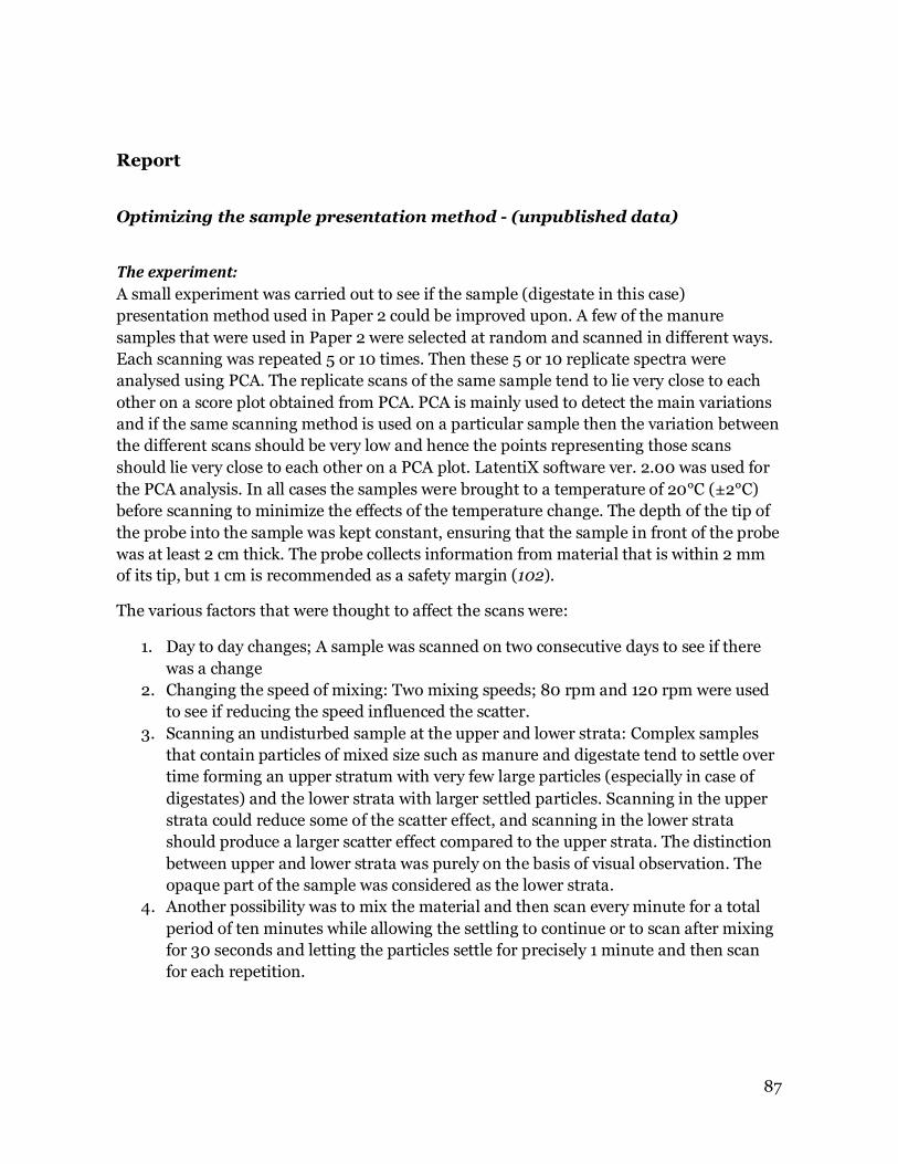
87
Report
Optimizing the sample presentation method - (unpublished data)
The experiment:
A small experiment was carried out to see if the sample (digestate in this case)
presentation method used in Paper 2 could be improved upon. A few of the manure
samples that were used in Paper 2 were selected at random and scanned in different ways.
Each scanning was repeated 5 or 10 times. Then these 5 or 10 replicate spectra were
analysed using PCA. The replicate scans of the same sample tend to lie very close to each
other on a score plot obtained from PCA. PCA is mainly used to detect the main variations
and if the same scanning method is used on a particular sample then the variation between
the different scans should be very low and hence the points representing those scans
should lie very close to each other on a PCA plot. LatentiX software ver. 2.00 was used for
the PCA analysis. In all cases the samples were brought to a temperature of 20°C (±2°C)
before scanning to minimize the effects of the temperature change. The depth of the tip of
the probe into the sample was kept constant, ensuring that the sample in front of the probe
was at least 2 cm thick. The probe collects information from material that is within 2 mm
of its tip, but 1 cm is recommended as a safety margin (102).
The various factors that were thought to affect the scans were:
1. Day to day changes; A sample was scanned on two consecutive days to see if there
was a change
2. Changing the speed of mixing: Two mixing speeds; 80 rpm and 120 rpm were used
to see if reducing the speed influenced the scatter.
3. Scanning an undisturbed sample at the upper and lower strata: Complex samples
that contain particles of mixed size such as manure and digestate tend to settle over
time forming an upper stratum with very few large particles (especially in case of
digestates) and the lower strata with larger settled particles. Scanning in the upper
strata could reduce some of the scatter effect, and scanning in the lower strata
should produce a larger scatter effect compared to the upper strata. The distinction
between upper and lower strata was purely on the basis of visual observation. The
opaque part of the sample was considered as the lower strata.
4. Another possibility was to mix the material and then scan every minute for a total
period of ten minutes while allowing the settling to continue or to scan after mixing
for 30 seconds and letting the particles settle for precisely 1 minute and then scan
for each repetition.

88
Results:
1. Day to day changes: The first principal component easily separated the scans
according to the day they were scanned although the same sample was used (Figure
A. 1). One reason could be due to sample degradation over the two day period of
scanning, but the degradation would be minimal as the sample was refrigerated
between the scans. Nevertheless, there is a variation and one way of building this
variation into a model would be to scan the samples on at least three different days
and then use the averaged spectra to build the model.
Figure A. 1: Day to day variation. The scans from day 1 are in dark blue while the scans from day 2 are in dark red.
2. Changing the mixing speed: There was no clear distinction between the two mixing
speeds (Figure A.2).
Figure A. 2: Mixing speed at 80 rpm is represented in dark blue while 120 rpm is represented by points in dark red.
-4 -3 -2 -1 0 1 2 3 4 5 6
-0.4
-0.3
-0.2
-0.1
0
0.1
0.2
0.3
0.4
0.5
Scores PC#1 (99.096%)
PCA Scores [Model 6]
Score
s P
C#2 (
0.7
84%
)
-1.5 -1 -0.5 0 0.5 1
-0.2
-0.15
-0.1
-0.05
0
0.05
0.1
0.15
0.2
Scores PC#1 (97.763%)
PCA Scores [Model 3]
Score
s P
C#2 (
1.7
74%
)
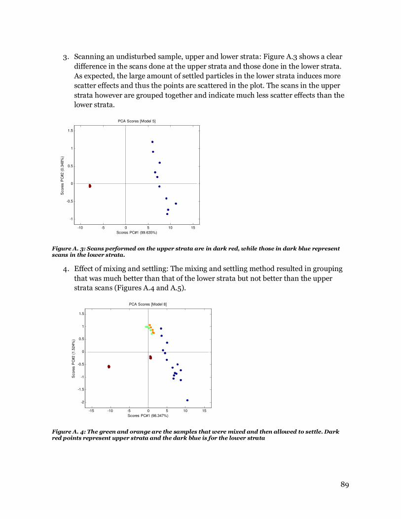
89
3. Scanning an undisturbed sample, upper and lower strata: Figure A.3 shows a clear
difference in the scans done at the upper strata and those done in the lower strata.
As expected, the large amount of settled particles in the lower strata induces more
scatter effects and thus the points are scattered in the plot. The scans in the upper
strata however are grouped together and indicate much less scatter effects than the
lower strata.
Figure A. 3: Scans performed on the upper strata are in dark red, while those in dark blue represent scans in the lower strata.
4. Effect of mixing and settling: The mixing and settling method resulted in grouping
that was much better than that of the lower strata but not better than the upper
strata scans (Figures A.4 and A.5).
Figure A. 4: The green and orange are the samples that were mixed and then allowed to settle. Dark red points represent upper strata and the dark blue is for the lower strata
-10 -5 0 5 10 15
-1
-0.5
0
0.5
1
1.5
Scores PC#1 (99.635%)
PCA Scores [Model 5]
Score
s P
C#2 (
0.3
48%
)
-15 -10 -5 0 5 10 15
-2
-1.5
-1
-0.5
0
0.5
1
1.5
Scores PC#1 (98.347%)
PCA Scores [Model 8]
Score
s P
C#2 (
1.5
24%
)

90
Figure A. 5: Difference between the mixing types and scans in the lower strata. Dark blue represents the lower strata, yellow and dark red represent mixing and then settling.
The results from this preliminary test show the importance of sample presentation. In
conclusion, the best grouping was with the samples scanned in the upper strata of the
undisturbed sample (Figure A.3). But this condition is difficult to emulate in anaerobic
digesters where the contents have to be mixed to ensure good contact between the
microbial population and the substrate, especially in case of CSTRs. The next best option
was to mix and allow the solids to settle for a while before scanning (Figures A.4 and A.5),
this can be recreated in a large scale reactor (Figure A.6) where samples can be run out of
the reactor in pipes as described in (47). The sample can be pumped through the pipe for a
period long enough to remove any remnants of old samples in the pipe. Instead of the
vertical option described in (47), the NIR probe can be affixed to a horizontal portion of the
sampling pipe where the fresh sample can now be allowed to settle for a short while and
then the relatively clear upper strata can be scanned by the NIRS. But, this method is
difficult to define with precision, as settling times with substrates such as digestate is
hardly ideal and vary depending on a lot of factors.
-8 -6 -4 -2 0 2 4
-0.8
-0.6
-0.4
-0.2
0
0.2
0.4
0.6
0.8
Scores PC#1 (98.962%)
PCA Scores [Model 15]
Score
s P
C#2 (
0.7
33%
)
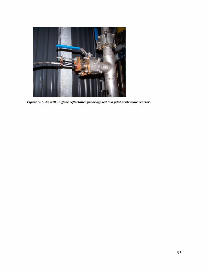
91
Figure A. 6: An NIR - diffuse reflectance probe affixed to a pilot-scale scale reactor.
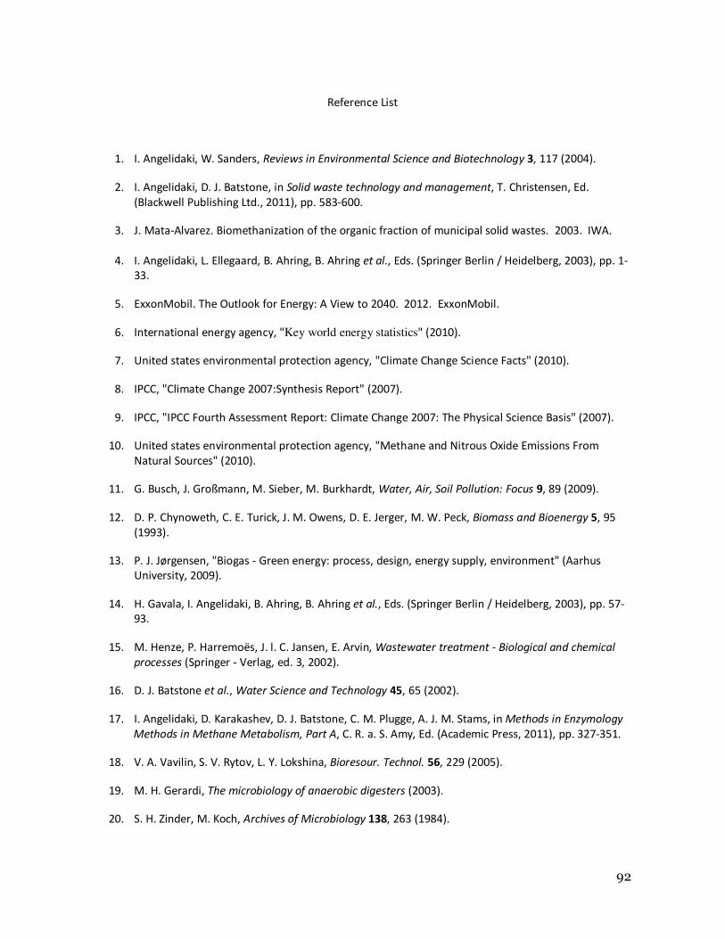
92
Reference List
1. I. Angelidaki, W. Sanders, Reviews in Environmental Science and Biotechnology 3, 117 (2004).
2. I. Angelidaki, D. J. Batstone, in Solid waste technology and management, T. Christensen, Ed. (Blackwell Publishing Ltd., 2011), pp. 583-600.
3. J. Mata-Alvarez. Biomethanization of the organic fraction of municipal solid wastes. 2003. IWA. 4. I. Angelidaki, L. Ellegaard, B. Ahring, B. Ahring et al., Eds. (Springer Berlin / Heidelberg, 2003), pp. 1-
33.
5. ExxonMobil. The Outlook for Energy: A View to 2040. 2012. ExxonMobil.
6. International energy agency, "Key world energy statistics" (2010).
7. United states environmental protection agency, "Climate Change Science Facts" (2010).
8. IPCC, "Climate Change 2007:Synthesis Report" (2007).
9. IPCC, "IPCC Fourth Assessment Report: Climate Change 2007: The Physical Science Basis" (2007).
10. United states environmental protection agency, "Methane and Nitrous Oxide Emissions From Natural Sources" (2010).
11. G. Busch, J. Großmann, M. Sieber, M. Burkhardt, Water, Air, Soil Pollution: Focus 9, 89 (2009).
12. D. P. Chynoweth, C. E. Turick, J. M. Owens, D. E. Jerger, M. W. Peck, Biomass and Bioenergy 5, 95 (1993).
13. P. J. Jørgensen, "Biogas - Green energy: process, design, energy supply, environment" (Aarhus University, 2009).
14. H. Gavala, I. Angelidaki, B. Ahring, B. Ahring et al., Eds. (Springer Berlin / Heidelberg, 2003), pp. 57-93.
15. M. Henze, P. Harremoës, J. l. C. Jansen, E. Arvin, Wastewater treatment - Biological and chemical
processes (Springer - Verlag, ed. 3, 2002).
16. D. J. Batstone et al., Water Science and Technology 45, 65 (2002).
17. I. Angelidaki, D. Karakashev, D. J. Batstone, C. M. Plugge, A. J. M. Stams, in Methods in Enzymology
Methods in Methane Metabolism, Part A, C. R. a. S. Amy, Ed. (Academic Press, 2011), pp. 327-351.
18. V. A. Vavilin, S. V. Rytov, L. Y. Lokshina, Bioresour. Technol. 56, 229 (2005).
19. M. H. Gerardi, The microbiology of anaerobic digesters (2003).
20. S. H. Zinder, M. Koch, Archives of Microbiology 138, 263 (1984).

93
21. A. M. Nielsen, PhD Thesis, University of Southern Denmark (2009).
22. Y. Chen, J. J. Cheng, K. S. Creamer, Bioresour. Technol. 99, 4044 (2008).
23. B. Ahring, M. Sandberg, I. Angelidaki, Applied Microbiology and Biotechnology 43, 559 (1995).
24. D. T. Hill, R. D. Holmberg, Biological Wastes 23, 195 (1988).
25. H. B. Nielsen, H. Uellendahl, B. K. Ahring, Biomass and Bioenergy 31, 820 (2007).
26. H. F. Jacobi, C. R. Moschner, E. Hartung. Use of near infrared spectroscopy in monitoring of volatile fatty acids in anaerobic digestion. 60(2), 339-346. 2009.
27. P. F. Pind, I. Angelidaki, B. K. Ahring, Biotechnol. Bioeng. 82, 791 (2003).
28. I. Angelidaki, B. K. Ahring, Water Res. 28, 727 (1994).
29. L. M. Safley Jr, P. W. Westerman, Biological Wastes 34, 133 (1990).
30. H. F. Jacobi, C. R. Moschner, E. Hartung, Bioresour. Technol. 102, 4688 (2011).
31. A. J. Ward, PhD Thesis, University of Bangor (2008).
32. W. F. Owen, D. C. Stuckey, J. Healy, L. Y. Young, P. L. McCarty, WATER RES. 13, 485 (1979).
33. N. V. Gunaseelan, Bioresour. Technol. 98, 1270 (2007).
34. H. F. Jacobi, S. Ohl, E. Thiessen, E. Hartung, Bioresour. Technol. 103, 162 (2012).
35. J. Petersen, P. Sørensen, "Fertilizer value of nitrogen in animal manures -Basis for determination of a legal substitution rate" (Det Jordbrugsvidenskabelige fakultet, Aarhus university, 2008).
36. I. Angelidaki, B. K. Ahring, Water Science and Technology 41, 189 (2000).
37. K. Boe, I. Angelidaki, Water Res. 43, 166 (2009).
38. D. Tilman, J. Hill, C. Lehman, Science 314, 1598 (2006).
39. A. Prochnow et al., Bioresour. Technol. 100, 4931 (2009).
40. M. Hansson, A. Nordberg, I. Sundh, B. Mathisen, Water Science and Technology 45, 255 (2002).
41. M. Hansson, A. Nordberg, B. Mathisen, Water Science and Technology 48, 9 (2003).
42. I. Angelidaki, B. K. Ahring, Applied Microbiology and Biotechnology 38, 560 (1993).
43. S. K. Bhattacharya, G. F. Parkin, Journal (Water Pollution Control Federation) 61, 55 (1989).
44. M. J. Adams, Chemometrics in analytical spectroscopy (The Royal Society of Chemistry, ed. 2, 2004).
45. A. J. Ward, A. L. Nielsen, H. B. Møller, Sensors 11, 4830 (2011).

94
46. H. Andree, M. Dolud, T. Hügle Baltic biorefinery symposium (2005).
47. A. J. Ward, C. S. Raju, H. B. Møller, Conference proceedings, Ramiran (2010).
48. P. Williams, K. Norris, Near-infrared technology in the agricultural and food industries (American association of cereal chemists Inc., 1987).
49. Å. Nordberg et al., Water Science and Technology 41, 1 (2000).
50. B. M. Nicolaï et al., Postharvest Biology and Technology 46, 99 (2007).
51. I. Karaman, Masters Thesis, Ízmir Institute of Technology (2008).
52. H. Spanjers, J. B. Van Lier, Water Science and Technology 53, 63 (2006).
53. G. Reich, Advanced drug delivery reviews 57, 1109 (2005).
54. B. Stuart, Infrared spectroscopy: Fundamentals and applications (John Wiley and Sons Ltd., 2004).
55. M. S. Dhanoa, S. J. Lister, R. J. Barnes, Applied Spectroscopy 49, 765 (1995).
56. K. H. Esbensen, Multivariate data analysis - in practice. An introduction to multivariate data
analysis and experimental design (CAMO, ed. 5, 2009).
57. M. Sjostrom, S. Wold, W. Lindberg, J. A. Persson, H. Martens, Anal. Chim. Acta 150, 61 (1983).
58. N. J. D. Nagelekerke, Biometrika 78, 691 (1991).
59. D. F. Malley, C. McClure, P. D. Martin, K. Buckley, W. P. McCaughey, Communications in Soil Science
and Plant Analysis 36, 455 (2005).
60. C. J. Lomborg, J. B. Holm-Nielsen, P. Oleskowicz-Popiel, K. H. Esbensen, Bioresour. Technol. 1711 (2009).
61. A. Schievano, M. Pognani, G. D'Imporzano, F. Adani, Bioresour. Technol. 99, 8112 (2008).
62. J. M. Triolo, S. G. Sommer, H. B. Møller, M. R. Weisbjerg, X. Y. Jiang, Bioresour. Technol. 102, 9395 (2011).
63. J. Forejtova et al., Czech Journal of Animal Science 50, 47 (2005).
64. D. J. Richards, L. K. Ivanova, D. J. Smallman, B. Zheng, International workshop on hydro-physico-mechanics of landfills (2005).
65. H. J. G. Jung, J. F. S. Lamb, Biomass & Bioenergy 27, 365 (2004).
66. J. B. Holm-Nielsen, H. Andree, H. Lindorfer, K. H. Esbensen, Journal of Near Infrared Spectroscopy 15, 123 (2007).
67. Camo Software AS. The Unscrambler methods. 2006. 68. W. Wu, B. Walczak, D. L. Massart, K. A. Prebble, I. R. Last, Anal. Chim. Acta 315, 243 (1995).
95
69. S. Wold, K. Esbensen, P. Geladi, Chemometrics and Intelligent Laboratory Systems 2, 37 (1987).
70. R. G. Brereton, Analyst 125, 2125 (2000).
71. B. Møller, Journal of the Institute of Brewing 110, 18 (2004).
72. S. Wold, M. Sjöström, L. Eriksson, Chemometrics and Intelligent Laboratory Systems 58, 109 (2001).
73. T. Næs, T. Isaksson, T. Fearn, T. Davies, A user-friendly guide to multivariate calibration and
classification (NIR Publications, 2007).
74. S. Wold et al., J. Chemometrics 23, 67 (2009).
75. L. Nørgaard et al., Applied Spectroscopy 54, 413 (2000).
76. R. De Maesschalck, D. Jouan-Rimbaud, D. L. Massart, Chemometrics and Intelligent Laboratory
Systems 50, 1 (2000).
77. G. Wang, H. N. Gavala, I. V. Skiadas, B. K. Ahring, Waste Management 29, 2830 (2009).
78. P. Weiland, Applied Biochemistry and Biotechnology 109, 263 (2003).
79. T. Al Seadi, "Danish centralised biogas plants - plant descriptions" (Bioenergy department, Universityof Southern Denmark, 2000).
80. H. B. Møller, S. G. Sommer, B. K. Ahring, Biomass and Bioenergy 26, 485 (2004).
81. N. Nesse, J. Wallick, J. M. Harper, Biotechnol. Bioeng. 19, 323 (1977).
82. D. Lee, V. N. Owens, A. Boe, P. Jeranyama, "Composition of herbaceous biomass feedstocks" (South Dakota State University, 2007).
83. L. da Costa Sousa, S. P. Chundawat, V. Balan, B. E. Dale, Current Opinion in Biotechnology 20, 339 (2009).
84. J. Pérez, J. Muñoz-Dorado, T. de la Rubia, J. Martínez, International Microbiology 5, 53 (2002).
85. E. Bruni, A. P. Jensen, I. Angelidaki, Bioresour. Technol. 101, 8713 (2010).
86. F. Carvalheiro, L. C. Duarte, F. M. Girio, Journal of Scientific & Industrial Research 67, 849 (2008).
87. M. Hjorth, K. Granitz, A. P. S. Adamsen, H. B. Moller, Bioresour. Technol. 102, 4989 (2011).
88. A. T. W. M. Hendriks, G. Zeeman, Bioresour. Technol. 100, 10 (2009).
89. V. B. Agbor, N. Cicek, R. Sparling, A. Berlin, D. B. Levin, Biotechnology Advances 29, 675 (2011).
90. M. J. Taherzadeh, K. Karimi, International Journal of Molecular Sciences 9, 1621 (2008).
91. J. Weil et al., Applied Biochemistry and Biotechnology 68, 21 (1997).
92. D. Yang, Y. Zheng, R. Zhang, ASABE annual international meeting (2009).
96
93. P. L. Beltrame, P. Carniti, A. Visciglio, Bioresour. Technol. 39, 165 (1992).
94. A. U. Buranov, G. Mazza, Industrial Crops and Products 28, 237 (2008).
95. Y. Zheng, Z. Pan, R. Zhang, Int J Agric & Biol Eng 2, 51 (2009).
96. D. L. Crawford, R. L. Crawford, Enzyme and Microbial Technology 2, 11 (1980).
97. D. Cullen, Journal of Biotechnology 53, 273 (1997).
98. R. P. Overend, E. Chornet, J. A. Gascoigne, Philosophical Transactions of the Royal Society of
London. Series A, Mathematical and Physical Sciences 321, 523 (1987).
99. R. Rafique et al., Energy 35, 4556 (2010).
100. W. Qiao et al., Renewable Energy 36, 3313 (2011).
101. B. Pickworth, J. Adams, K. Panter, O. E. Solheim, Water Science and Technology 54, 101 (2006).
102. A. Larsen,Personal communication.

Department of Engineering Aarhus University Edison, Finlandsgade 22 8200 Aarhus N Denmark
Tel.: +45 4189 3000
Chitra Sangaraju Raju, Optimization of the anaerobic digestion process by substrate pre-treatment and the application of NIRS, 2012