optimization of polynomial expressions by using the
TRANSCRIPT

Optimization of Polynomial Expressions by using the Extended Dual Polarity
Dragan Janković (a), Radomir S. Stanković (a), Claudio Moraga (b),
(a) Faculty of Electronics, University of Niš, Serbia and Montenegro, [email protected]; [email protected]
(b) European Centre for Soft Computing, Mieres, Spain Faculty of Computer Science, University of Dortmund, Germany
Abstract – A method for optimization of polynomial expressions in terms of fixed polarities for
discrete functions is presented. The method is based on the principle of extended dual polarity, which provides a simple way of ordering polarities to obtain an effective way of finding the optimal polarity. The method still implies exhaustive search, but it is an optimized search, which may be expressed in very simple rules. Experimental results illustrate the effectivity of the proposed method.
Keywords – Switching functions, Multiple-valued functions, Reed-Muller expressions, Polynomial
expressions, Fixed-polarity expressions 1. INTRODUCTION Polynomial expressions are a form of representations of discrete functions that provides for compact representations of large functions. Their definition and exploitation is derived from the classical engineering approach consisting of decomposition of complex systems into combinations of subsystems that are simpler or whose behavior is well documented. In the case of polynomial expressions, a given function is decomposed into a linear combination of some suitably selected complete sets of basis functions. In this case, dealing with function values of a given function f is replaced by dealing with coefficients for f assigned to the basis functions. Reducing the number of non-zero coefficients, usually denoted as optimization of the representation for f, reduces complexity of dealing with f, and therefore, it is among the main goals in theory and practice of discrete functions. In attempting to derive polynomial expressions with minimum number of coefficients, a variety of different polynomial expressions have been defined in the literature, most of them for switching functions, i.e., binary valued functions of binary variables, see for example [27] and references given therein. However, many of these expressions are extended or generalized to multiple-valued input binary-valued output (MVB) functions [3,9,25,26] and multiple-valued input multiple-valued output (MV) functions [4,6,8,16,20,21]. A brief review of these extensions is discussed in [19] where related references are provided. Polynomial expressions for binary functions and their generalizations to MVB and MV functions are defined in terms of different expansion rules with respect to their variables [28], which can be alternatively interpreted as choosing different sets of basis functions [29]. Within some of these classes of expressions, a further optimization can be performed by using literals of different polarity for variables, which leads to a

variety of fixed- and mixed-polarity expressions [6,7,8]. This way of optimization of polynomial expressions can be interpreted as reordering and sifting of basis functions in terms of which the representations are defined. It can be applied, under an appropriate definition of negation, to both bit-level expressions, with whatever binary or MV digits used in encoding values for variables, and word-level expressions, in which case variables take integer values. The chief problem in this approach is that given a function f, we do not know how to select a priori the polarity of variables to get the optimal polynomial expression in the number of non-zero coefficients count. Solutions are offered through heuristic algorithms [23,25] or brute force search methods yielding to the so-called polarity matrices [8]. Recall that a polarity matrix is a matrix whose rows are coefficients in all possible fixed polarity expressions for a given function f. In the first case, the efficiency of the method is assured by reducing the search space at the price of an increased number of coefficients. In the second case, advantage is taken of the recursive structure of polarity matrices, which structure originates in the definition of the polarity for variables. This observation applies generally, whatever may be the way of representing either binary, MVB or MV functions and sets of coefficients in their polynomial expressions, as tables or vectors, arrays of cubes, or relating them to paths in decision diagrams, etc. In this paper, we present a method to determine the optimal polynomial expressions of discrete functions for different polarities of variables. In the method discussed, it is assumed that a function is represented by a set of cubes, which are processed independently of each other. Therefore, the complexity of the method is determined by the number of cubes rather than the number of variables. This feature was the main motivation for selecting cubes as data structure to represent functions. However, the presented method can be easily adapted an performed over other data structures, as vectors or decision diagrams for instance. The presentation in the paper is given for MV functions as the most general class of considered functions with most of examples for quaternary functions. However, all the algorithms proposed can be equally applied to MVB and binary functions after specifying the corresponding parameters, as will be illustrated by the examples provided, below. 1.1 Background work and Motivation Besides seeking for generality (up to some extent), and the fact that there are phenomena naturally described by MVB and MV functions, another reason to study the optimization of polynomial expressions for MV functions is that these functions can be efficiently exploited in solving optimization problems for binary switching functions that are prevalent in nowadays practice. Some of these applications are briefly discussed in [9]. For example, a well-known approach to represent a multiple-output Boolean function is to treat its output part as a single multiple-valued variable and convert it to a single-output characteristic function. Such an approach is used in ESPRESSO-MV [22] and in MVSIS [10]. Other applications of multiple-valued logic include design of PLAs with input decoders [24], optimization of finite state machines [1], [28], testing [11] and verification [5]. Different representations for multiple-valued input two-valued output functions are defined including a generalization of disjunctive normal form or Sum-of-product (SOP) expressions and Kronecker and Pseudo-Kronecker expressions for binary input binary output switching functions [26,27]. These expressions can be uniformly considered as linear combinations of basis functions over GF(2). The basis functions used in these expressions are expressible as products of multiple-valued (MV) literals. Minimization of these expressions is crucial in practical applications [25].
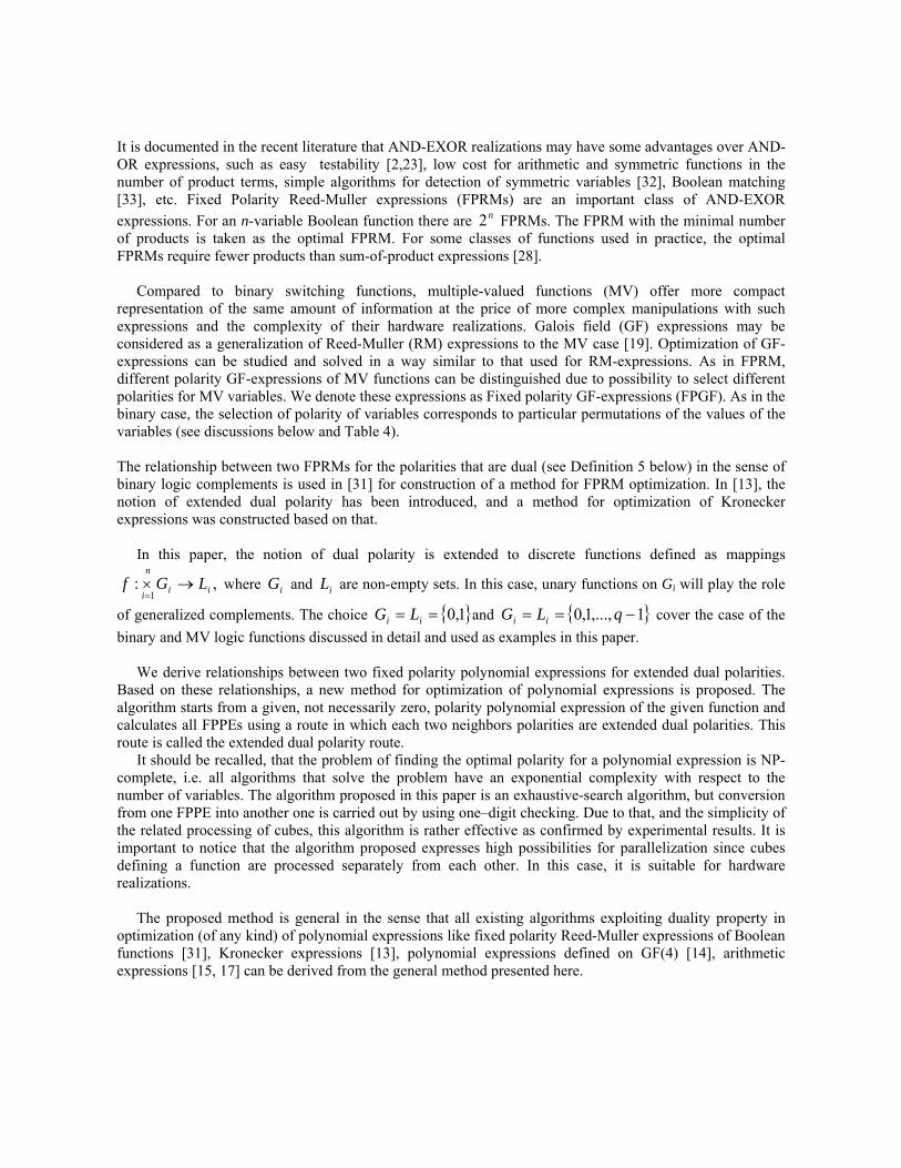
It is documented in the recent literature that AND-EXOR realizations may have some advantages over AND-OR expressions, such as easy testability [2,23], low cost for arithmetic and symmetric functions in the number of product terms, simple algorithms for detection of symmetric variables [32], Boolean matching [33], etc. Fixed Polarity Reed-Muller expressions (FPRMs) are an important class of AND-EXOR expressions. For an n-variable Boolean function there are n2 FPRMs. The FPRM with the minimal number of products is taken as the optimal FPRM. For some classes of functions used in practice, the optimal FPRMs require fewer products than sum-of-product expressions [28]. Compared to binary switching functions, multiple-valued functions (MV) offer more compact representation of the same amount of information at the price of more complex manipulations with such expressions and the complexity of their hardware realizations. Galois field (GF) expressions may be considered as a generalization of Reed-Muller (RM) expressions to the MV case [19]. Optimization of GF-expressions can be studied and solved in a way similar to that used for RM-expressions. As in FPRM, different polarity GF-expressions of MV functions can be distinguished due to possibility to select different polarities for MV variables. We denote these expressions as Fixed polarity GF-expressions (FPGF). As in the binary case, the selection of polarity of variables corresponds to particular permutations of the values of the variables (see discussions below and Table 4). The relationship between two FPRMs for the polarities that are dual (see Definition 5 below) in the sense of binary logic complements is used in [31] for construction of a method for FPRM optimization. In [13], the notion of extended dual polarity has been introduced, and a method for optimization of Kronecker expressions was constructed based on that.
In this paper, the notion of dual polarity is extended to discrete functions defined as mappings
,:1 ii
n
iLGf →×
= where iG and iL are non-empty sets. In this case, unary functions on Gi will play the role
of generalized complements. The choice { }1,0== ii LG and { }1,...,1,0 −== qLG ii cover the case of the binary and MV logic functions discussed in detail and used as examples in this paper.
We derive relationships between two fixed polarity polynomial expressions for extended dual polarities.
Based on these relationships, a new method for optimization of polynomial expressions is proposed. The algorithm starts from a given, not necessarily zero, polarity polynomial expression of the given function and calculates all FPPEs using a route in which each two neighbors polarities are extended dual polarities. This route is called the extended dual polarity route.
It should be recalled, that the problem of finding the optimal polarity for a polynomial expression is NP-complete, i.e. all algorithms that solve the problem have an exponential complexity with respect to the number of variables. The algorithm proposed in this paper is an exhaustive-search algorithm, but conversion from one FPPE into another one is carried out by using one–digit checking. Due to that, and the simplicity of the related processing of cubes, this algorithm is rather effective as confirmed by experimental results. It is important to notice that the algorithm proposed expresses high possibilities for parallelization since cubes defining a function are processed separately from each other. In this case, it is suitable for hardware realizations.
The proposed method is general in the sense that all existing algorithms exploiting duality property in
optimization (of any kind) of polynomial expressions like fixed polarity Reed-Muller expressions of Boolean functions [31], Kronecker expressions [13], polynomial expressions defined on GF(4) [14], arithmetic expressions [15, 17] can be derived from the general method presented here.

2. BASIC DEFINITIONS As indicated above, the presentation will be given for multiple-valued functions. This section gives some basic definitions and notions from the theory of fixed polarity representation of MV functions used as examples in the paper. 2.1 Polynomial expressions Definition 1: (Polynomial expressions (PE)) Each n-variable q-valued function { } { }1,...,1,01,...,1,0: −→− qqf n given by the truth-vector
Tqnff ],,[
10 −= KF can be represented by a polynomial expression defined in matrix notation as
FTX )()(),,( 1 nnxxf n =K (1) where
[ ]12
11)( −
=⊗= q
iii
n
ixxxn LX ,
and
)1()(1TT
n
in
=⊗= , ( ) 1)1()1( −= XT ,
where ⊗ denotes the Kronecker product, and the basic transform matrix T(1) is defined as the inverse of X(1), assuming that the symbolic notation for columns of X(1) is replaced by the corresponding truth-vectors. Addition and multiplication (and, hence, exponentiation) are defined in the used algebraic structure. Mostly, this is the structure of vector spaces over GF(2) or GF(q), however, it is possible to use also other algebraic structures, as for instance these considered in [4], [34], permitting definition of polarity of variables. As examples of polynomial expressions, Reed-Muller expressions, Kronecker expressions, Galois field expressions over GF(4) and arithmetic expressions are defined in the Appendix. Here, we give a numeric example for functions in GF(4).
Example 1: The GF(4) expression of a two-variable four-valued function f, (given) defined by the truth-vector [ ]T1,0,0,1,2,2,2,2,1,1,0,3,1,1,3,0=F is given by
( ) ( ) ( )( ) ( ) ( ) ( ) ( ) ( ) 2
31
32
21
22
21
21
32121
32
22221
333
32322),(
xxxxxxx
xxxxxxxxxf
⋅+⋅⋅+⋅⋅+⋅
+⋅⋅+⋅⋅+⋅+⋅+⋅=
The coefficients are elements of the corresponding FPGF spectrum, which is therefore given by
]0,0,1,0,3,3,0,3,3,0,2,0,3,2,2,0[=S . The zero elements in the spectrum correspond to the missing terms
in the expansion. Notice that there are 12 non-zero elements in the truth-vector and 9 in the above
polynomial expansion for f.
Recall that the operations (addition (+) and multiplication (• )) are in GF(4), defined as follows:

Addition in GF(4) + 0 1 2 3 0 0 1 2 3 1 1 0 3 2 2 2 3 0 1 3 3 2 1 0
Multiplication in GF(4)
• 0 1 2 3 0 0 0 0 0 1 0 1 2 3 2 0 2 3 1 3 0 3 1 2
The polarity of variables )4(GFxi ∈ , 2,1=i , is defined as 1+= xx . 2.2 Optimization of polynomial expressions Optimization of polynomial expression, viewed as the determination of an expression with the minimum number of non-zero coefficients (i.e. the number of terms), can be done by introducing different polarities for the variables. The representations thus produced are so-called fixed polarity polynomial expressions (FPPE) where each variable ix appears as either the positive or the negative literal. i.e., as uncomplemented or complemented, but not both at the same time. Definition 2: (Complement) For a q-valued variable x, there are q-1 complements xc given as
1,...,1 , −=⊕= qccxxc . xc is usually denoted as a variable x with a polarity c. (With this notation, the complement used in Example
1 corresponds to 1=c , and can be written as x1 )
Polarity vector P is introduced to denote the polarity of variables and correspondingly the polarity of a representation [35]. Definition 3: (Polarity vector) For an n-variable q-valued function f, the polarity vector ( ) { }1,,1,0 ,,...,1 −∈= qppp in LP is a vector of length n, whose elements specify the polarity of variables in FPPE for an n-variable function f, i.e., jpi =
shows that to the i-th variable the j-th complement is assigned and written as ij x .
Fixed polarity polynomial expressions (FPPEs) are uniquely characterized by specifying decomposition rules assigned to variables i.e. by specifying the polarity vectors. Definition 4: (Fixed polarity expressions) Each n-variable q-valued function f given by the truth-vector T
qnff ],,[ 10 −= KF can be represented by the
following FPPE if the polarity is ),,( 1 nppp L= ,

FTX )()(),,( 1 nnxxf ppn
><><=K where
( ) ( )[ ]12
11)(
−
=
>< ⊗=q
ip
ip
ip
n
i
p xxxn iii LX ,
)1()(1
><
=
>< ⊗= ipn
i
p n TT .
Therefore, FPPEs can be given by the vector of coefficients, usually denoted as spectrum, >< pS defined as
FTS )(npp ><>< = .
Example 2: The fixed polarity GF(4) (FPGF) expression of a two-variable four-valued function f, discussed in Example 1, for a polarity )3,2(=p is given by
( ) ( )( ) ( ) ( )( ) ( ) ( ) ( ) 2
331
231
232
321
2
22
321
22
321
2
32
31
222
31
221
33
3
322),(
xxxxx
xxxx
xxxxxxf
⋅+⋅+⋅⋅
+⋅+⋅⋅
+⋅⋅+⋅⋅+=
The corresponding FPGF spectrum is given by ]0,0,1,3,3,1,3,0,3,2,0,0,0,0,0,2[3,2 =><S . Notice that >< 3,2S
has 8 zero-coefficients, meanwhile >< 1,2S has only 6.
3. EXTENDED DUAL POLARITY In minimization of FPPE with respect to the number of non-zero coefficients count, it appears convenient to exploit the notion of the dual polarity [13], the extended dual polarity, and the related dual polarity and the extended dual polarity vectors. The term dual polarity is used in the Boolean domain to denote two polarity vectors which differ in only one bit.
Definition 5: (Dual polarity) In the case of binary functions, for a given polarity ),,,,,,( 111 niii pppppp KK +−= , { })1,0( ∈ip the polarity ),,,,,,(' 111 niii pppppp KK +−= is the dual polarity.
Example 3: Dual polarities for the polarity )0,1(=p are the polarities (0,0) and (1,1).
In the multiple-valued domain, the term dual polarity will be called the extended dual polarity [13].
Definition 6: (Extended dual polarity) For a given polarity ),,,,,,( 111 niii pppppp KK +−= , { })1,...,1,0( −∈ qpi the polarity )',,',',',,'(' 111 niii pppppp KK +−= is the extended dual polarity iff ijpp jj ≠= ,' and
ii pp ≠' .

Example 4: For four-valued functions the extended dual polarities for the polarity )0,1(=p are the polarities (0,0), (2,0), (3,0) , (1,1), (1,2), and (1,3). 3.1 Dual polarity route
The number of polarity vectors characterizing all possible FPPEs for an n-variable q-valued function is nq . It is possible to order these nq polarities such that each two successive polarities are the extended dual polarities. We denote this order as the extended dual polarity route. Traversing of a q-valued n-dimensional hypercube can generate one of many possible extended dual polarity routes. Table 1 gives the number of dual polarity routes for different values of q and n.
Table 1: Number of dual polarity routes q n No polarities No routes 2 2 2 2
1 2 3 4
2 4 8 16
2 8
144 91392
3 3
1 2
3 9
6 1512
4 4
1 2
4 16
24 22394880
Example 5: Two different dual polarity routes for q=4 and n=2 are given by the sequences of polarity vectors (00)-(01)-(02)-(03)-(13)-(12)-(11)-(10)-(20)-(21)-(22)-(23)-(33)-(32)-(31)-(30) and (00)-(01)-(11)-(10)-(20)-(21)-(22)-(12)-(02)-(03)-(13)-(23)-(33)-(32)-(31)-(30). These routes are shown in Figure 1. Example 6: An extended dual polarity route generated by using traversal of a four-valued three-dimensional hypercube is given by
(000)—(001)—(002)—(003)—(013)—(012)—(011)—(010)—(020)—(021)—(022)—(023)—(033)—(032)—(031)—(030)—(130)—(131)—(132)—(133)—(123)—(122)—(121)—(120)—(110)—(111)—(112)—(113)—(103)—(102)—(101)—(100)—(200)—(201)—(202)—(203)—(213)—(212)—(211)—(210)—(220)—(221)—(222)—(223)—(233)—(232)—(231)—(230)—(330)—(331)—(332)—(333)—(323)—(322)—(321)—(320)—(310)—(311)—(312)—(313)—(303)—(302)—(301)—(300). An extended dual polarity route can be constructed by using the recursive procedure route(level, direction) given in Figure 2 for the particular case q = 4. Extension to an arbitrary q is straightforward. Extended dual polarity route will be produced if the procedure is called with arguments equal 0, i.e., as route(0,0).
4. RELATIONSHIPS BETWEEN DUAL POLARITY EXPRESSIONS
Denote by S , ><gS , and ><hS the vectors of coefficients in FPPEs for the polarities zero, g, and h, respectively, assuming that g and h are two distinct extended dual polarities.

Therefore, the spectrum for zero polarity is FTS )(n= , and spectra for two different polarities g and h are
FTS )(ngg ><>< = , FTS )(nhh ><>< = ,
where g and h differ in the i-th coordinate ( )niii ppppppg LL ,,,,, 1121 +−= , ( )niii pppppph LL ,,',,, 1121 +−= .
Since ( ) ><−><= hh n STF1
)( , the relationship between ><gS and ><hS is given by
( ) )()()()()( 1 nnnnn hhggg ><−><><><>< ⋅⋅== STTFTS . Further,
BTA
TTT
TT
⊗⊗=
⎟⎠⎞
⎜⎝⎛ ⊗⊗⊗⎟
⎠⎞
⎜⎝⎛⊗=
⊗=
><
><
+=
><><−
=
><
=
><
)1(
)1()1()1(
)1()(
1
1
1
1
i
jij
j
p
pn
ij
ppi
j
pn
j
g n
where ⎟⎠⎞
⎜⎝⎛⊗= ><
−
=)1(
1
1
jpi
jTA and ⎟
⎠⎞
⎜⎝⎛ ⊗= ><
+=)1(
1
jpn
ijTB .
Similarly,
BTA
TTT
TT
⊗⊗=
⎟⎠⎞
⎜⎝⎛ ⊗⊗⊗⎟
⎠⎞
⎜⎝⎛⊗=
⊗=
><
><
+=
><><−
=
><
=
><
)1(
)1()1()1(
)1()(
'1
'1
1
1
i
jij
j
p
pn
ij
ppi
j
pn
j
h n
Figure 1: Dual polarity routes.

Due to the Kronecker structure of the transform matrix )(nh><T and the features of the Kronecker product
(assuming consistent dimensions), the inverse transform matrix ( ) 1)( −>< nhT is given as
( ) ( ) 11 BTAT −−><−−>< ⊗⊗=1'1 )1()( iph n .
Finally, ( ) ( )( ) ( )( )
( )( )( )( ) in
ppi
pp
pphg
ii
ii
iinn
−
−><><−
−−><><−
−−><−><−><><
⊗⊗=
⊗⊗=
⊗⊗⊗⊗=⋅
ITTI
BBTTAA
BTABTATT 1
1'1
11'1
1'11
)1()1(
)1()1(
)1()1()()(
where kI is the identity matrix of order qk.
void route(int level, int direction) { if( direction == 0) { if(level == no_variable)
{ -- out new polarity vector h } else { h[level] = 0; route(level+1, 0); h[level] = 1; route(level+1, 1); h[level] = 2; route(level+1, 0); h[level] = 3; route(level+1, 1); }
} else { if(level == no_variable)
{ -- out new polarity vector h } else { h[level] = 3; route(level+1, 0);
h[level] = 2; route(level+1, 1); h[level] = 1; route(level+1, 0); h[level] = 0; route(level+1, 1); } } }
Figure 2: Procedure route().

The matrix ><gS is a nicely structured sparse matrix which expresses a property that we will exploit for the generation of a processing rule for transforming the coefficients of one polarity polynomial expression into the coefficients of another extended dual polarity polynomial expression for the given function, i.e.
( )( )( ) ><−
−><><−
>< ⋅⊗⊗= hin
ppi
g ii SITTIS1'
1 )1()1( . (2) The following example illustrates conversion of coefficients in the polynomial expansion for a given polarity into a required dual polarity for the most familiar binary case. In the case of MV functions that would be the extended dual polarity coefficients as it will be seen in further examples below. For simplicity of matrix notation, the example is given for binary valued functions. Example 7: Let a Boolean function f be given by the truth-vector [ ]T0110011101111100=F . The fixed polarity Reed-Muller (FPRM) expression of f for the polarity p=(0110) is given by the spectrum
[ ]T10110010001111110110 =><S while the FPRM expresion of f for the polarity p'=(0010) is given by the
spectrum [ ]T10110001111111000010 =><S . Polarities p and p' are dual polarities, since they differ only in the second bit, and, therefore,
><
−
>< ⋅⎟⎟⎟
⎠
⎞
⎜⎜⎜
⎝
⎛⊗⎟
⎟
⎠
⎞
⎜⎜
⎝
⎛⎟⎟⎠
⎞⎜⎜⎝
⎛⎥⎦
⎤⎢⎣
⎡⎥⎦
⎤⎢⎣
⎡⊗= 0010
2
1
10110
1110
1101
SIIS
where 1I and 2I are the identity matrices of order 2 and 4, respectively. Therefore,
[ ]
[ ].1011001000111111
0011010011111110
1000000000000000010000000000000000100000000000000001000000000000100010000000000001000100000000000010001000000000000100010000000000000000100000000000000001000000000000000010000000000000000100000000000010001000000000000100010000000000001000100000000000010001
1011000111111100
1000010000100001
1011
10010110
=
⎥⎥⎥⎥⎥⎥⎥⎥⎥⎥⎥⎥⎥⎥⎥⎥⎥⎥⎥⎥⎥⎥⎥
⎦
⎤
⎢⎢⎢⎢⎢⎢⎢⎢⎢⎢⎢⎢⎢⎢⎢⎢⎢⎢⎢⎢⎢⎢⎢
⎣
⎡
⋅
⎥⎥⎥⎥⎥⎥⎥⎥⎥⎥⎥⎥⎥⎥⎥⎥⎥⎥⎥⎥⎥⎥⎥
⎦
⎤
⎢⎢⎢⎢⎢⎢⎢⎢⎢⎢⎢⎢⎢⎢⎢⎢⎢⎢⎢⎢⎢⎢⎢
⎣
⎡
=
⋅
⎟⎟⎟⎟⎟
⎠
⎞
⎜⎜⎜⎜⎜
⎝
⎛
⎥⎥⎥⎥
⎦
⎤
⎢⎢⎢⎢
⎣
⎡
⊗⎥⎦
⎤⎢⎣
⎡⊗⎥
⎦
⎤⎢⎣
⎡=>< TS

5. PROCESSING RULES A relationship between two extended dual FPPEs given by (2) will be the starting point for the derivation of a processing rule which should be applied to all the terms in FPPE for a given polarity to determine the FPPE for another extended dual polarity.
Let nii
i mmmm 11
1 +−= be a term in the FPPE of a function f for the polarity
),,,,( 111 niii ppppph LL +−= . The value of the coefficient in the FPPE for f for the term m is )(mh><S . The process assumes that non-zero terms of f are processed separately in determining FPPEs. Since
processing means multiplication with the rows of the transform matrices, and a row may have several non-zero entries, a given term m for a specified polarity p may produce few new terms in the FPPE of the function f for the extended dual polarity ),,',,( 111 niii pppppg LL +−= depending on the values of ip
and ip' . Thus, m generates new terms in ><gS representing coefficients in FPPE for f for the polarity g.
The value of the extended dual FPPE on a newly generated term is given by )(mv h><S where ν strongly depends on the considered extended dual polarities g and h, which dependency can be conveniently expressed in matrix notation by a matrix ( )( ) 1' )1()1(
−><><= ii pp TTL . The rules to process terms in FPPE for the polarity h to determine new terms in the FPPE for the polarity g can be derived from the matrix L as stated in the following theorem formulated for the general case of q-valued functions.
Theorem 1: Let a matrix L relating product terms in FPPEs for the polarities h and g be given as
⎥⎥⎥⎥⎥⎥
⎦
⎤
⎢⎢⎢⎢⎢⎢
⎣
⎡
=
−−−−−−
−−−−−−
−−
−−
1,12,11,10,1
1,22,21,20,2
1,12,11,10,1
1,02,01,00,0
qqqqqq
qqqqqq
llllllll
llllllll
L
L
MMOMM
L
L
L .
The processing rules to generate new terms in FPPE for the polarity g from terms in FPPE for the polarity h are determined as follows: Recall that n
iii mmmm 1
11 +−= ;
if kmi = then generate ni
i tmm 11
1 +− 1,,0 ,1,,0 −=−= qkqt LL
and use ktlv ,= as the scaling factor in )(mv h><S
Proof: Rewrite the equation (2) in the form ( )( )( ) ( ) ><><
−−><
−
−><><−
>< ⋅=⋅⊗⊗=⋅⊗⊗= hhini
hin
ppi
g ii SRSILISITTIS 11'
1 )1()1( . (3)
The orders of the matrices , ],[ 1, −= ijil IL and in−I are ,r , 1A
−= iqq and inB qr −= , respectively.
From (3), ],[ , jir=R where wuji lr ,, ≡ for
⎩⎨⎧
−=++=−=++=
,1,...,0,,1,...,0,
BBB
ABB
rwrqrjrurqri
ββααβα

i.e.
1,,0 ),,,,,,,,,(),,,,,,,,,(
11121
11121
−=⎩⎨⎧
==
−+−
−+−
qzzzzwzzzjzzzuzzzi
i
nnii
nnii
L
LL
LL
(4)
u, w ∈ {0, 1, … q-1} Consider contribution of a term ),,,,,,( 111 nii mmkmmm LL +−= in ><hS to ><gS . The non-zero coefficients in the m-th column of the matrix R are the elements with the decimal index
1,,0 ),,,,,,,( 111 −== +− qtmmtmmd nii LLL .
This means that the term m from ><hS contributes to terms in ><gS with the decimal index d. The value of contribution to these terms ><hvS , according to (4), is given as
><><>< ⋅=⋅=⋅ hkt
hmd
h lrv SSS ,, . End of the Proof.
Example 8: The contribution of the term m=(0,3) in >< 2,1S , for the (1,2) polarity FPRM of function f given in Example 1 (the truth vector is F=[0,3,1,1,3,0,1,1,2,2,2,2,1,0,0,1]), to >< 1,1S , for the (1,1) polarity FPRM, is given by (3,1,2,0,0,0,0,0,0,0,0,0,0,0,0,0) (see Figure 3).
⎥⎥⎥⎥⎥⎥⎥⎥⎥⎥⎥⎥⎥⎥⎥⎥⎥⎥⎥⎥⎥⎥⎥
⎦
⎤
⎢⎢⎢⎢⎢⎢⎢⎢⎢⎢⎢⎢⎢⎢⎢⎢⎢⎢⎢⎢⎢⎢⎢
⎣
⎡
⎥⎥⎥⎥⎥⎥⎥⎥⎥⎥⎥⎥⎥⎥⎥⎥⎥⎥⎥⎥⎥⎥⎥
⎦
⎤
⎢⎢⎢⎢⎢⎢⎢⎢⎢⎢⎢⎢⎢⎢⎢⎢⎢⎢⎢⎢⎢⎢⎢
⎣
⎡
⎥⎥⎥⎥⎥⎥⎥⎥⎥⎥⎥⎥⎥⎥⎥⎥⎥⎥⎥⎥⎥⎥⎥
⎦
⎤
⎢⎢⎢⎢⎢⎢⎢⎢⎢⎢⎢⎢⎢⎢⎢⎢⎢⎢⎢⎢⎢⎢⎢
⎣
⎡
+
⎥⎥⎥⎥⎥⎥⎥⎥⎥⎥⎥⎥⎥⎥⎥⎥⎥⎥⎥⎥⎥⎥⎥
⎦
⎤
⎢⎢⎢⎢⎢⎢⎢⎢⎢⎢⎢⎢⎢⎢⎢⎢⎢⎢⎢⎢⎢⎢⎢
⎣
⎡
=
⎥⎥⎥⎥⎥⎥⎥⎥⎥⎥⎥⎥⎥⎥⎥⎥⎥⎥⎥⎥⎥⎥⎥
⎦
⎤
⎢⎢⎢⎢⎢⎢⎢⎢⎢⎢⎢⎢⎢⎢⎢⎢⎢⎢⎢⎢⎢⎢⎢
⎣
⎡
⇒
⎥⎥⎥⎥⎥⎥⎥⎥⎥⎥⎥⎥⎥⎥⎥⎥⎥⎥⎥⎥⎥⎥⎥
⎦
⎤
⎢⎢⎢⎢⎢⎢⎢⎢⎢⎢⎢⎢⎢⎢⎢⎢⎢⎢⎢⎢⎢⎢⎢
⎣
⎡
0000000000000213
0000000000003000
0000000000003000
0012323031120031
0012323031123031
1001222211031130
F >< 2,1S m m contribution of m to >< 1,1S
Figure 3: Term contribution Above contributions of the term m are calculated by the following:

Starting polarity is <1,2>; Calculated polarity is <1,1>; Matrix ( )⎥⎥⎥⎥
⎦
⎤
⎢⎢⎢⎢
⎣
⎡
=⋅=−><><
1000310020101231
112 GGL ;
Therefore, the term m = (0 3) with value 3, contribute to the terms (0 0), (0 1) and (0 2) with values given as 3 times the corresponding value from the fourth column in matrix L i.e. 3*1= 3, 3*2 = 1 and 3*3=2, respectively.
Using the above theorem, it is possible to derive all the existing methods for optimization of polynomial expressions which exploit the dual polarity property as well as to produce new methods for determination of some new polynomial expressions. 6. DUAL POLARITY BASED OPTIMIZATION ALGORITHM Since for an n-variable q-valued function f, there are qn possible FPPEs, in an exhaustive-search optimization algorithms all of nq fixed polarity polynomial expressions should be calculated. Usually, the starting point in determination of each of nq FPPEs is the truth-vector for f. In a class of algorithms which exploit dual
polarity feature [2], [3], [4], again these nq FPPEs are calculated, but the truth-vector is the starting point only for the first FPPE. Any other FPPE is calculated starting from an arbitrary FPPE. Figure 4 illustrates the way of traversing from one to another polarity in the classical approach and by exploiting the extended dual polarity. In classical approach all of nq FPPEs are calculated from the truth vector (Figure 4-a). In dual-polarity based approach only first FPPE is calculated from the truth vector while other FPPEs are calculated from the previously calculated dual-polarity FPPE (Figure 4-b) which reduce the computational complexity due to the features of the dual poarity route.
a)
. . .
. . .
f
p=(0,0,...,0) p=(0,0,...,1) p=(0,0,...,0) p q q q=( -1, -1, ... , -1)
b)
f
p=(0,0,...,0) p=(0,0,...,1) p=(0,0,...,0) p q q q=( -1, -1, ... , -1)
Figure 4: Optimization algorithms: a) classic b) dual-polarity based

In Section 3 is explained how to construct an extended dual polarity route. The main idea of the proposed algorithm is that all nq FPPE are constructed along the extended dual polarity route, i.e., each FPPE is calculated starting from an initial extended dual polarity FPPE. An open question is the determination of a processing rule for processing of terms from one FPPE to produce terms in another extended dual polarity FPPE. Theorem 1 gives the processing rule for arbitrary FPPEs. From this theorem, it follows that it is possible to calculate all FPPEs by using the method for transforming a given FPPE into the extended dual polarity FPPE along the route without repetitive calculations. Therefore, we can perform the optimization of FPPE, i.e., construction of all FPPEs and subsequent selection of the FPPE with the minimum number of non-zero coefficients, by using an effective exhaustive-search algorithm consisting of the following steps.
1. Initialization: - Set the polarity vector p to )0,,0,0( L=p - Calculate the spectrum >< pS - Set minC = the number of non-zero coefficients in >< pS
2. Determine the next extended dual polarity p’, according to the recursive route.
3. List all the terms for >< pS .
4. For each term calculate the contribution to the spectrum >< 'pS by using the processing rule derived from Theorem 1.
5. Delete terms whose value is equal to zero after summation of contributions of the processed terms. 6. Calculate the total number of non-zero coefficients min'C .
If minmin' CC < then minmin 'CC = .
7. Stop if all polarities have been treated. Otherwise go to Step 2.
The algorithm, as formulated above, starts from the zero polarity FPPE, but it can start from any other polarity. The initial FPPE representing the input in the algorithm should be calculated from any specification of the given function (for instance, truth-vector, cubes, decision diagrams) by using any of the existing methods. Then, the terms in this initial FPPE should be specified by cubes which are the input in the algorithm.
For instance, we may want to start from the FPPE for the zero polarity for a given function f , which may
be calculated from the truth vector for f. For this task we can also use some known methods, for example, the tabular technique [5]. It is interesting to notice that the algorithm proposed has high possibilities for parallelization. Each processor performs the method along a piece of the extended dual polarity route. The extended dual polarity route can be divided into z subroutes if the number of parallel processors is z. In what follows, the theory presented in this section will be illustrated by examples of Galois field GF(4) expressions.

7. FIXED POLARITY GF(4) EXPRESSIONS In this section, we consider optimization of fixed polarity polynomial expressions of functions defined on GF(4) by using the extended dual polarity method. The optimization of a GF(4) expression is possible by using different complements. There are three complements for a variable in GF(4) denoted by 3,2,1 , =ixi and defined as 3,2,1 , =+= iixxi . In FPGFs, the use of complements for a variable requires permutation of columns in the basic GF(4) transform matrix corresponding to that variable. Table 2 shows complements and the corresponding basic transform matrices as well as their inverses that are used to define the operators for calculating coefficients in GF-expressions.
Table 2: Complements in GF(4) and basic transform matrices.
Variable Transform Inverse transform
⎥⎥⎥
⎦
⎤
⎢⎢⎢
⎣
⎡=
3210
x ⎥⎥⎥
⎦
⎤
⎢⎢⎢
⎣
⎡=
1111321023100001
G ( )⎥⎥⎥
⎦
⎤
⎢⎢⎢
⎣
⎡=−
1231132111110001
1G
⎥⎥⎥
⎦
⎤
⎢⎢⎢
⎣
⎡=
2301
1x ⎥⎥⎥
⎦
⎤
⎢⎢⎢
⎣
⎡=><
1111230132010010
1G ( )⎥⎥⎥
⎦
⎤
⎢⎢⎢
⎣
⎡=
−><
1231132100011111
11G
⎥⎥⎥
⎦
⎤
⎢⎢⎢
⎣
⎡=
1032
2 x ⎥⎥⎥
⎦
⎤
⎢⎢⎢
⎣
⎡=><
1111103210230100
2G ( )⎥⎥⎥
⎦
⎤
⎢⎢⎢
⎣
⎡=
−><
1111000112311321
12G
⎥⎥⎥
⎦
⎤
⎢⎢⎢
⎣
⎡=
0123
3 x ⎥⎥⎥
⎦
⎤
⎢⎢⎢
⎣
⎡=><
1111012301321000
3G ( )⎥⎥⎥
⎦
⎤
⎢⎢⎢
⎣
⎡=
−><
0001111113211231
13G
The following example illustrates GF(4) fixed polarity polynomial expressions.
Example 9: The fixed polarity GF (FPGF) expression of a two-variable four-valued function f in Example 1 for the polarity )1,2(=p is given by
( ) ( ) ( ) ( ) ( ) ( ) ( ) ( )( ) ( ) ( ) ( ) ( ) ( ) ( )2
131
231
232
121
22
121
2
21
232
11
222
11
22
11
21
221
3
33222),(
xxxxxxx
xxxxxxxxxxf
⋅++⋅⋅+⋅
++⋅⋅+⋅⋅+⋅⋅+⋅+=
The coefficients are elements of the corresponding FPGF spectrum, which is therefore is given by
]0,0,1,1,3,0,1,1,3,3,2,2,0,0,0,2[1,2 =><S .
The FPGF of a four-valued function f can be represented by a set of four-valued (n+1)-tuples, consisting of terms and the corresponding function values on these terms. For simplicity, literals for variables in terms are replaced by their indices. A variable that is present in a product term in the i-th complemented form is replaced by i, and 0 replaces an absent variable. Therefore, the FPGF for the function f and the assumed
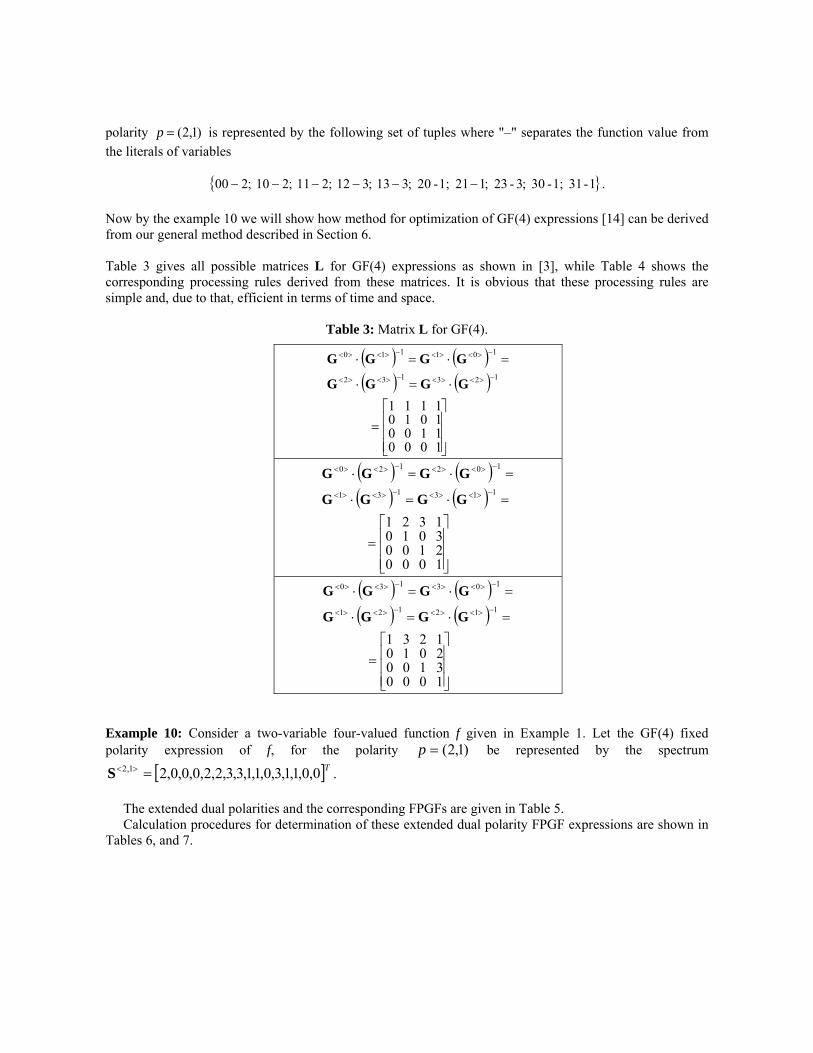
polarity )1,2(=p is represented by the following set of tuples where "–" separates the function value from the literals of variables
{ }1-31 1;-30 ;3-23 ;121 1;-20 ;313 ;312 ;211 ;210 ;200 −−−−−− .
Now by the example 10 we will show how method for optimization of GF(4) expressions [14] can be derived from our general method described in Section 6. Table 3 gives all possible matrices L for GF(4) expressions as shown in [3], while Table 4 shows the corresponding processing rules derived from these matrices. It is obvious that these processing rules are simple and, due to that, efficient in terms of time and space.
Table 3: Matrix L for GF(4).
( ) ( )( ) ( )
⎥⎥⎥
⎦
⎤
⎢⎢⎢
⎣
⎡=
⋅=⋅
=⋅=⋅−><><−><><
−><><−><><
1000110010101111
123132
101110
GGGG
GGGG
( ) ( )( ) ( )
⎥⎥⎥
⎦
⎤
⎢⎢⎢
⎣
⎡=
=⋅=⋅
=⋅=⋅−><><−><><
−><><−><><
1000210030101321
113131
102120
GGGG
GGGG
( ) ( )( ) ( )
⎥⎥⎥
⎦
⎤
⎢⎢⎢
⎣
⎡=
=⋅=⋅
=⋅=⋅−><><−><><
−><><−><><
1000310020101231
112121
103130
GGGG
GGGG
Example 10: Consider a two-variable four-valued function f given in Example 1. Let the GF(4) fixed polarity expression of f, for the polarity )1,2(=p be represented by the spectrum
[ ]T0,0,1,1,3,0,1,1,3,3,2,2,0,0,0,21,2 =><S . The extended dual polarities and the corresponding FPGFs are given in Table 5. Calculation procedures for determination of these extended dual polarity FPGF expressions are shown in
Tables 6, and 7.
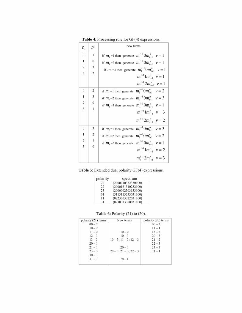
Table 4: Processing rule for GF(4) expressions.
ip ip' new terms
0
1
2
3
1
0
3
2
if im =1 then generate ni
i mm 11
1 0 +− 1=v
if im =2 then generate ni
i mm 11
1 0 +− 1=v
if im =3 then generate ni
i mm 11
1 0 +− 1=v
ni
i mm 11
1 1 +− 1=v
ni
i mm 11
1 2 +− 1=v
0
1
2
3
2
3
0
1
if im =1 then generate ni
i mm 11
1 0 +− 2=v
if im =2 then generate ni
i mm 11
1 0 +− 3=v
if im =3 then generate ni
i mm 11
1 0 +− 1=v
ni
i mm 11
1 1 +− 3=v
ni
i mm 11
1 2 +− 2=v
0
1
2
3
3
2
1
0
if im =1 then generate ni
i mm 11
1 0 +− 3=v
if im =2 then generate ni
i mm 11
1 0 +− 2=v
if im =3 then generate ni
i mm 11
1 0 +− 1=v
ni
i mm 11
1 1 +− 2=v
ni
i mm 11
1 2 +− 3=v
Table 5: Extended dual polarity GF(4) expressions.
polarity spectrum 20 22 23 01 11 31
(2000010332330100) (2000131310232100) (2000002303133100) (3113113333031100) (0223003322031100) (0230333300031100)
Table 6: Polarity (21) to (20). polarity (21) terms New terms polarity (20) terms
00 – 2 10 – 2 11 – 2 12 – 3 13 – 3 20 – 1 21 – 1 23 – 3 30 – 1 31 – 1
10 – 2 10 – 3
10 – 3; 11 – 3; 12 – 3
20 – 1 20 – 3; 21 – 3; 22 – 3
30– 1
00 – 2 11 – 1 13 – 3 20 – 3 21 – 2 22 – 3 23 – 3 31 – 1

Table 7: Polarity (21) to (22).
polarity (21) terms new terms polarity (22) terms 00 – 2 10 – 2 11 – 2 12 – 3 13 – 3 20 – 1 21 – 1 23 – 3 30 – 1 31 – 1
10 – 1 10 – 1
10 – 3; 11– 1; 12 – 2
20 – 3 20 – 3; 21 – 1; 22 – 2
30 – 3
00 –2 10 – 1 11 – 3 12 – 1 13 – 3 20 – 1 22 – 2 23 – 3 30 – 2 31 – 1
7.1 Efficiency of the method Features of the proposed method and its efficiency have been examined by a series of experiments the sample of which is presented in the Section 9. Experimental results confirmed the efficiency of the method compared to the related methods. For calculation of all FPRMs based on the truth vector, the inverse transform matrix and its complemented forms are used. The number of zero coefficients in these matrices for GF(4) is 3 (see Table 2). On the other side, for the method proposed in this paper, all FPRMS are calculated but calculations are performed by using L matrices (for GF(4) see Table 3). The number of zero coefficients in these matrices is 7. Increasing of number of zero coefficients in processing matrices leads to the reduction in the number of operations required for calculation of FPRMs. 8. PARTICULAR CASES In this section, in the manner used in the previous section, we will show that methods for generation fixed-polarity Kronecker expressions [13], fixed polarity Reed-Muller expressions [31] as well as fixed polarity arithmetic expressions [15] can be derived as particular cases of the extended dual polarity based optimization algorithm described in Section 6. 8.1 Kronecker expressions for binary valued functions
In [13] is proposed a method for optimization of Kronecker expressions. This method can be considered as a particular case of the present method as can be seen from Table 8 shows processing rules for all possible cases for Kronecker expressions of Boolean functions [2] derived by the specification of parameters in the general method discussed above. Note that polarity 2 denotes Shannon expansion while polarity 0 and 1 denote positive Davio and negative Davio expansions, respectively. Also, for all cases 1=v . 8.2 Fixed polarity Reed-Muller expressions
Fixed polarity Reed-Muller (FPRM) expressions can be optimized by using the dual polarity property as given in [31] which can be viewed as a particular case of the general method discussed above.

Table 9 shows processing rules for the FPRM of Boolean functions. As for the Kronecker expressions, in this case it is also 1=v .
Table 8: Processing rule for Kronecker expressions.
ip ip' new terms
0 1 1 0
if im =1 then generate ni
i mm 11
1 0 +−
0 2 2 0
if im =0 then generate ni
i mm 11
1 1 +−
1 2 if im =1 then set im =0
if im =0 then generate ni
i mm 11
1 1 +−
2 1 if im =0 then set im =1
if im =1 then generate ni
i mm 11
1 0 +−
Table 9: Processing rule for FPRM expressions of Boolean functions.
ip ip' new terms
0 1 1 0
if im =0 then generate ni
i mm 11
1 1 +−
8.3 Fixed polarity arithmetic expressions
Dual polarity is used in [15] for optimization of fixed polarity arithmetic expressions (FPAE). This method can be also derived as a particular case of the general method.
Table 10 shows processing rules for fixed polarity arithmetic expressions FPAE [4].
Table 10: Processing rule for arithmetic expressions.
ip ip' new terms
0
1
1
0
if im =1 then a) generate ni
i mm 11
1 0 +−
and set 1=v . b) generate n
ii mm 1
11 1 +−
and set 1−=v .
9. EXPERIMENTAL RESULTS In this section, we present some experimental results estimating features and efficiency of the proposed algorithm for minimization of FPPEs. As example we give results for FPGF expressions for functions defined on GF(4), FPAE of Boolean functions, and Kronecker expressions.

9.1 FPGFs We developed a program in C for determination of optimal FPGF expression for an arbitrary four-valued function represented by minterms. The experiments were carried out on a 1GHz PC Celeron with 128Mb of main memory and all runtimes are given in CPU seconds. Table 11 compares the runtimes for optimization of FPGF expressions by the CTT method introduced in [5] (columns CTT) with the extended dual polarity based algorithm proposed in [3] that, as shown above, can be derived from the method given in this paper (columns Dual). We consider randomly generated four-valued functions with 25% and 75% of non-zero minterms (columns 25% and 75%, respectively) where the number of four-valued variables n ranges from 4 to 7. Columns %d show the ratio (CTT – Dual)/ Dual where CTT and Dual refer to the methods in [5] and [3], respectively. CPU time reduction given in columns %d are shown in Figure 5. The extended dual polarity based algorithm is faster than CTT due to the simplified processing by using the extended dual polarity property. This ratio increases with increasing number of variables. Furthermore, the number of non-zero minterms has smaller influence upon the runtime of the proposed algorithm as compared to CTT.
Table 11: CPU times for calculation of FPGF by Dual polarity and CTT . 25% 75%
N Dual CTT %d Dual CTT %d 4 5 6 7
0.04 0.54 10.34 251.32
0.06 2.17 89.75 3922.05
-33.33 -75.11 -88.48 -93.59
0.4 0.56 12.69 299.28
0.16 6.33 266.54 12429.99
-75.0 -91.15 -95.24 -97.59
-100
-90
-80
-70
-60
-50
-40
-30
-20
-10
04 5 6 7
d-25% d-75%
Figure 5: Reduction of CPU times for calculation of FPGF by Dual polarity method compared with CTT
method

9.2 Kronecker expressions In this subsection, we present some experimental results estimating features and efficiency of the extended dual polarity based method for optimization of Kronecker expressions. Table 12 and Figure 6 give the runtimes (in milliseconds) for the Kronecker expression optimization for the same functions as for the FPAEs optimization. The new column denoted as (012) represents the functions taking the value 1 at the first three minterms and the value 0 at other minterms. The conclusion is the same as in the case of FPAEs, i.e., the number of minterms strongly influences the runtime of this algorithm.
Table 12: CPU times for calculation of Kronecker expressions, q=2.
n (012) 25% 75% 5 6 7 8 9 10 11
<0.01 <0.01 0.04 0.25 1.41 8.19 47.93
0.01 0.04 0.52 6.24 73.27
890.00 10831.21
0.01 0.05 0.56 5.93 75.19 917.09
11199.35
0.01
0.1
1
10
100
1000
10000
1000005 6 7 8 9 10 11
(1 2 3) 25% 75%
Figure 6: CPU times (in milliseconds) for calculation of Kronecker expressions, q=2
We expect that dual polarity based methods for optimization of other classes of polynomial expressions, which can be derived from the proposed method will express the same or similar features.

9.3 FPAEs In this subsection, we present the same experimental results as in previous subsections, however, this time estimating features and efficiency of the extended dual polarity based method for the minimization of fixed polarity arithmetic expressions. Table 13 compares the runtimes for optimization of arithmetic expressions by the Tabular technique in [12] (columns ATT) with the algorithm that is derived from the method proposed in this paper (columns Dual). We consider the simple functions taking the value 1 at the first three minterms (0,1,2), randomly generated functions with 25% of all possible minterms, and randomly generated functions with 75% of all possible minterms, where the number of variables n ranges from 7 to 12. Columns %d show the ratio (Dual – ATT)/ATT where ATT and Dual refer to the method in [12] and the proposed algorithm, respectively. These columns are shown in Figure 7, too.
It can be concluded that the number of minterms strongly influences the runtime of the extended dual polarity based algorithm, but it is faster than ATT.
Table 13: CPU times for calculation of arithmetic expressions, q=2.
(012) 25% 75% n ATT Dual %d ATT Dual %d ATT Dual %d 7 8 9 10 11 12
<0,01 0,02 0,08 0,3 1,14 4,62
<0,01 <0,01 <0,01 0,01 0,04 0,16
- -50 -87,5 -96,67 -96,49 -96,53
0,03 0,16 1,04 6,12
36,66 222,22
<0,01 <0,01 <0,01 0,03 0,07 0,30
-66,67 -93,75 -99,04 -99,51 -99,81 -99,86
0,09 0,52 3,01 17,91 108,29 222,41
<0,01 0,01 0,01 0,03 0,11 0,35
-88,89 -98,08 -99,67 -99,83 -99,90 -99,84
-100
-90
-80
-70
-60
-50
-40
-30
-20
-10
07 8 9 10 11 12
(1 2 3) 25% 75%
Figure 7: Reduction of CPU times for calculation of arithmetic expressions, q=2 by Dual polarity method
compared with ATT method

10. CONCLUDING REMARKS In this paper we have proposed a general method for optimization of polynomial expressions by using the extended dual polarity property. We have introduced the notion of extended dual polarities as a extension of the very well known term, dual polarity, in Boolean algebra. Based on the extended dual polarity, we have shown dependencies between two extended dual polarity polynomial expressions. This dependency is used as a base for deriving the method. All existing methods which exploit the dual polarity property in optimization [13], [14], [15], [31] can be derived from our method as an particular cases. By using the proposed method it is possible to derive similar methods for optimization of other polynomial expressions. For all given cases the processing rules are simple and efficient. Due to that, although being an exhaustive-search method, the proposed method is effective. Experimental results are given to show the performance of the extended dual polarity methods.
The proposed optimization method works with minterms. An extension to work with disjoint cubes can be a promising direction, since a cube based tabular technique, which starts from disjoint cubes [18], is more efficient than similar techniques starting from minterms [30].
REFERENCES [1] De Micheli, G. D., Brayton, R., Sangiovanni-Vincentelli, A., “Optimal state assignment for finite state
machines”, IEEE Trans. on CAD/ICAS, Vol. CAD-4, No. 3, July 1985, 269-284. [2] Drechsler, R., Hengster, H., Schaefer, H., Hartman, J., Becker, B., “Testability of 2-Level AND/EXOR
Circuits”, in Journal of Electronic Testing, Theory and Application, Vol. 14, No. 3, June 1999, 173-192. [3] Dubrova, E.; Farm, P.; “A conjunctive canonical expansion of multiple-valued functions”, Proc. 32nd
IEEE International Symposium on Multiple-Valued Logic, May 15-18, 2002, 35 -38. [4] Dubrova, E.V., Muzio, J.C., “Generalized Reed-Muller canonical form for a multiple-valued algebra“,
Multiple-Valued Logic, An International Journal, Vol. 1, 1996, 65-84. [5] Dubrova, E., Sack, H., “Probabilistic verification of multiple-valued functions”, in Proc. 30th Int. Symp.
on Multiple-Valued Logic, May 2000, 461-466,. [6] Falkowski, B.J.; Cheng Fu; “Family of fast transforms over GF(3) logic”, Proc. 33rd Int. Symp. on
Multiple-Valued Logic, 2003., May 16-19 2003, 323 -328. [7] Falkowski, B.J.; Chip-Hong Chang; “Optimization of partially-mixed-polarity Reed-Muller expansions”,
Proc. Int. Symp. on Circuits and Systems, ISCAS '99, Vol. 1, May 30- June 2, 1999, Vol. 1, 383 -386.
[8] Falkowski, B.J.; Rahardja, S.; “Efficient computation of quaternary fixed polarity Reed-Muller expansions”, IEE Proc. Computers and Digital Techniques, Volume: 142 No. 5, Sept. 1995, 345 -352.
[9] Farm, P. Dubrova, E., Stankovic, R.S., Astola, J., "Conjunctive decomposition for multiple-valued input
binary-valued output functions", Proc. TISCP Workshop on Spectral Methods and Multirate Signal Processing, SMMSP'02, Toulouse, France, September 7-8, 2002, 227-234.

[10] Gao , M., Jiang ,J.-H., Jiang , Y., Li , Y., Sinha , S., Brayton, R., “MVSIS”, in Proc. Int. Workshop on Logic Synthesis, June 2001, 138-144.
[11] E. Dubrova. Multiple-valued logic synthesis and optimization. In Logic Synthesis and Verification,
Eds.: S. Hassoun and T. Sasao, pages 89-114, Kluwer Academic Publishers, 2002. [12] Janković, D., “Tabular technique for the fixed polarity arithmetic transform calculation”, XLVII
Conference ETRAN, 2003, Herceg-Novi, Serbia and Montenegro (in Serbian). [13] Janković, D., Stanković, R.S., Moraga, C., “Optimization of Kronecker expressions using the extended
dual polarity property“, Proc. XXXVII International Scientific Conf, on Information, Communication and Energy Systems and Technologies, ICEST 2002, Nis, Yugoslavia, 749-752.
[14] Janković, D., Stanković, R.S., Moraga, C., “Optimization of GF(4) expressions using the extended dual
polarity property“,Proc. 33th Int. Symp. on Multiple-Valued Logic, Tokyo, Japan, May 2003, 50-56. [15] Janković, D., Stanković, R.S., Moraga, C., “Optimization of arithmetic expressions using the dual
polarity property“, 1st Balkan Conference in Informatics, BCI ‘2003, Thessaloniki, Greece, 2003, pp. 402-410.
[16] Janković, D., Stanković, R.S., Drechsler, R., “Efficient calculation of fixed polarity polynomial
expressions for multi-valued logic function“, Proc. 32nd Int. Symp. on Multiple-Valued Logic, Boston, USA, May 2002, 76-82.
[17] Janković, D., Stanković, R.S., Moraga, C.,"Arithmetic Expressions Optimization Using Dual Polarity
Property", Serbian Journal of Electrical Engineering, Vol. 1, No. 1, November 2003, pp. 71-80.
[18] Janković, D., Stanković, R.S., Drechsler, R., "Cube tabular technique for calculation of fixed polarity Reed-Muller expressions and applications'', Proc. of a Workshop on Computational Intelligence and Informational Technologies, June 20-21, Niš, 2001, 81-88.
[19] Karpovsky, M.G.; Stankovic, R.S.; Moraga, C., "Spectral techniques in binary and multiple-valued
switching theory. A review of results in the decade 1991-2000”, Proc. 31st Int. Symp. on Multiple-Valued Logic, May 22-24, 2001, 41 -46.
[20] Muzio, J.C., Wesselkamper, T.C., Multiple-valued Switching Theory, Adam Hilger, Bristol, 1986. [21] Rahardja, S.; Falkowski, B.J.; “Efficient algorithm to calculate Reed-Muller expansions over GF(4)”,
IEE Proc. Circuits, Devices and Systems, Vol. 148, No. 6 , Dec. 2001, 289 -295. [22] Rudel , R., Sangiovanni-Vincentelli, A., "Multiple-valued minimization for PLA optimization", IEEE
Trans. on CAD/ICAS, Vol. CAD-5, No. 9, Sept. 1987, 727-750. [23] Sarabi, A., Perkowski, M.A., “Fast exact and quasi-minimal minimization of highly testable fixed
polarity AND/XOR canonical networks”, Proc. Design Automation Conference, June 1992, 30-35.

[24] Sasao, T., "Multiple-valued logic and optimization of programmable logic arrays", IEEE Computer, Vol. 21, 1988, 71-80.
[25] Sasao, T., “EXMIN - A simplification algorithm for exclusive-or-sum-of-product expressions for
multiple-valued input two-valued output functions”, 20th Int. Symp. on Multiple-Valued Logic, Charlotte, North Carolina, May 23-25, 1990, 128-135.
[26] Sasao, T., “A transformation of multiple-valued input two-valued output functions and its application to
simplification of exclusive-or-sum-of-products expressions”, ISMVL-91, 1991, 270-279. [27] Sasao, T., Butler, J.T, "A design method for look-up table type FPGA by pseudo-Kronecker
expansions'', Proc. 24th Int. Symp. on Multiple-valued Logic, Boston, Massachusetts, May 25-27, 1994, 97-104.
[28] Sasao, T., Switching Theory for Logic Synthesis, Kluwer Academic Publishers, 1999. [29] Stankovic, R.S., Spectral Transform Decision Diagrams in Simple Questions and Simple Answers,
Nauka, Belgrade, 1998. [30] Tan, E.C., Yang, H., "Fast tabular technique for fixed-polarity Reed-Muller logic with inherent parallel
processes'', Int.J. Electronics, Vol.85, No.85, 1998, 511-520. [31] Tan, E.C., Yang, H., “Optimization of Fixed-polarity Reed-Muller circuits using dual-polarity
property”, Circuits Systems Signal Process, Vol. 19, No. 6, 2000, 535-548. [32] Tsai, C., Marek-Sadowska, M., “Generalized Reed-Muller forms as a tool to detect symmetries”, IEE
Proc. Computers and Digital Techniques, Vol. 141, No. 6, November 1994, 369-374. [33] Tsai, C., Marek-Sadowska, M., “Boolean functions classification via fixed polarity Reed-Muller forms”,
IEEE Trans.Comput., Vol. C-46, No. 2, February 1997, 173-186. [34] Stankovic, R.S., Jankovic, D., Moraga, C., “reed-Muller-Fourier versus Galois field representations of
four-valued logic functions”, Proc. 28th Int. Symp.On Multiple-Valued Logic, May 27-29, 1998, pp. 186-191.
[35] Green, D.H., “Dual forms of Reed_Muller expansions”, IEE Proc. Computers and Digital Techniques,
Vol 141, No. 3, 1994, pp. 184-192.

Appendix Examples of polynomial expressions for binary and multiple-value functions. A.1 Reed-Muller expressions Polynomial expression (1) defined over Galois field GF(2) is very well known as Reed-Muller expression of Boolean functions. All calculations are done in GF(2) i.e. operations addition and multiplication are addition modulo 2 and multiplication modulo 2, respectively. Reed-Muller expressions have the form
[ ] [ ] FFR ⎟⎠⎞
⎜⎝⎛
⎥⎦⎤
⎢⎣⎡⊗⎟
⎠⎞
⎜⎝⎛⊗=⎟
⎠⎞
⎜⎝⎛⊗⎟⎠⎞
⎜⎝⎛⊗=
==== 11011)1(1),,(
11111
n
ii
n
i
n
ii
n
in xxxxf K
where F is the truth vector of Boolean function f.
Example 11: Reed-Muller expression of a 2-variable Boolean function f, given by the truth-vector [ ]T1,1,1,0=F , is given by
[ ] [ ]( )211
2121
1101
110111),(
xxx
xxxxf
⊕=
⋅⎟⎠⎞
⎜⎝⎛
⎥⎦⎤
⎢⎣⎡⊗⎥⎦
⎤⎢⎣⎡⊗= F
A.2 Kronecker expressions
Kronecker expression of Boolean function f given by the truth vector F is given as
FTX ⎟⎠⎞
⎜⎝⎛⊗⎟⎠⎞
⎜⎝⎛⊗=
==
ii pn
i
pn
inxxf111 ),,( K
where [ ][ ][ ]⎪⎩
⎪⎨
⎧
===
=,2,,1,1,0,1
iii
ii
iip
pxxpxpx
iX
and
⎪⎪⎪
⎩
⎪⎪⎪
⎨
⎧
=⎥⎦
⎤⎢⎣
⎡
=⎥⎦
⎤⎢⎣
⎡
=⎥⎦
⎤⎢⎣
⎡
=
,2,1001
,1,1110
,0,1101
i
i
i
p
p
p
p
iT
The vector [ ] { }2,1,0 ,,,1 ∈= iT
n ppp KP determines the kind of expansions used for each variable where 0=ip denotes positive Davio expansion, 1=ip denotes negative Davio expansion and 2=ip denotes
Shannon expansion. Used operations are modulo 2 operations.

Example 12: Kronecker expression of a 2-variable Boolean function f, given by the truth-vector [ ]T0,1,1,0=F , for a vector [ ]T1,2=P is given by
[ ] [ ]( )21121
21121
1101
10011),(
xxxxx
xxxxxf
⊕⊕=
⋅⎟⎠⎞
⎜⎝⎛
⎥⎦⎤
⎢⎣⎡⊗⎥⎦
⎤⎢⎣⎡⊗= F
A.3 GF(4) expressions If q=4 and addition and multiplication are carried out in GF(4) (as specified in Example 1) then (1) represents GF-expressions for a 4-variable function. Exponentiation in GF(4) is defined in Table 14. Notice that if the Table 16 is viewed as a matrix whose rows correspond to the rows in the table, then this matrix is the inverse matrix for the basic GF(4) transform matrix.
Table 14: Exponentiation in GF(4).
0(.) 0 1(.) 2(.) 3(.) 0 1 0 0 0 1 1 1 1 1 2 1 2 3 1 3 1 3 2 1
Example 13: The basic GF(4) transform matrix is given as
⎥⎥⎥
⎦
⎤
⎢⎢⎢
⎣
⎡==
1111321023100001
)1( GT .
The GF(4) spectrum and the corresponding polynomial expression for a two-variable four-valued function f, given by the truth-vector [ ]T1,0,0,1,2,2,2,2,1,1,0,3,1,1,3,0=F are given as
( ) [ ]T0,0,1,0,0,3,0,3,1,1,1,0,3,2,2,0)1()1()( =⊗== FGGF2TS and
231
22
21
21
321
22121
32
22221 33322),( xxxxxxxxxxxxxxxxf ++++++++= ,
respectively. A.4 Arithmetic expressions Arithmetic expressions are closely related to Reed-Muller expressions since they are defined in terms of the same basis, however, with variables and function values interpreted as integers 0 and 1 instead of logic values. In this way, arithmetic expressions can be considered as integer counterparts of Reed-Muller expressions.
FAX )()(),,( 1 nnxxf n =K where
[ ]i
n
ixn 1)(
1=⊗=X , ⎥
⎦
⎤⎢⎣
⎡−
⊗== 11
01)(
1
n
inA ,
and addition and multiplication are arithmetic operations. )(nA represents the arithmetic transform matrix of order n.